Embed Size (px)
Citation preview

Real-Time Rendering and Acquisition
of Spherical Light Fields
Echtzeit-Rendering und Akquisitionspharischer Lichtfelder
Vom Fachbereich Elektrotechnik und Informatik derUniversitat Siegen
zur Erlangung des akademischen Grades
Doktor der Ingenieurwissenschaften(Dr.-Ing.)
genehmigte Dissertation
von
Dipl.-Inf. Severin Sonke Todt
Siegen – Juni 2009
1. Gutachter: Prof. Dr. A. Kolb2. Gutachter: Prof. Dr. G. GreinerVorsitzender: Prof. Dr. V. Blanz
Tag der mundlichen Prufung: 16. Juni 2009

Gedruckt auf alterungsbestandigem holz- und saurefreiem Papier.
Abstract
Image-based rendering techniques have proven to be a powerful alternative totraditional polygon-based computer graphics. This thesis presents a novel lightfield rendering technique which performs per-pixel depth correction of rays forhigh-quality light field reconstruction. The technique stores combined RGBand depth values in a parabolic 2D texture for every light field sample beingacquired at discrete positions in a uniform spherical setup. Image synthesisis implemented on the graphics processing unit within a customized fragmentprogram which extracts the correct image information from adjacent camerasfor each fragment by applying per-pixel depth correction of rays.
This dissertation demonstrates that the presented image-based renderingtechnique provides a significant improvement compared to previous approaches.Two different rendering implementations are explained which make use of theuniform parametrization to minimize disparity problems and ensure full sixdegrees of freedom for virtual view synthesis. While one rendering algorithmimplements an iterative refinement approach for rendering light fields with per-pixel depth correction, the other approach employs a raycaster which providessuperior rendering quality at moderate frame rates.
Graphics processing unit based per-fragment depth correction of rays, usedin both implementations, helps reducing ghosting artifacts to a non noticeableamount and provides a rendering technique that performs without exhaustivepre-processing for 3D object reconstruction.
The presented light field techniques open up for the implementation of ef-ficient and flexible rendering approaches. This work presents an efficient levelof detail rendering approach for light fields and introduces a flexible render-ing technique for remote access to light field representation in a web-basedclient-server application.
For the acquisition of spherical light fields with per-pixel depth a new ac-quisition system is presented which makes use of recent advances in 3D sensortechnology to acquire combined RGB and depth images directly.
iii


Zusammenfassung
Bildbasierte Renderingmethoden haben sich in der Vergangenheit als ef-fiziente Alternative zu traditionellen Renderingmethoden auf Polygonbasis er-wiesen. Diese Doktorarbeit prasentiert eine neue Lichtfeld-Renderingmethodedie unter Ausnutzung von pro Pixel Tiefenwerten eine hochqualitative Bildsyn-these in Echtzeit ermoglicht. Fur einen diskreten Satz an gleichmassig aufder Oberflache einer Kugelreprasentation angeordneter Samplepositionen spei-chert die Technik kombinierte RGB und Tiefenwerte in einer gemeinsamenparabolischen Textur. Die Bildsynthese erfolgt auf dem Grafikprozessor undist in einem angepassten Fragment Program umgesetzt, das zur Bestimmungder Fragment Farbe korrekte Bildinformationen aus benachbarten Samplepo-sitionen extrahiert.
Im Vergleich zu denen in der Vergangenheit vorgestellten Lichtfeldverfahrenstellt die in dieser Arbeit prasentierte Technik eine signifikante Verbesserungdar. Es werden zwei unterschiedliche Renderingverfahren dargestellt, die beidedie gleichmassige Samplingstruktur nutzen, um Disparitatsprobleme zu ver-meiden und virtuelle Ansichten mit sechs Freiheitsgraden zu ermoglichen.Wahrend das eine der Verfahren einen iterativen Ansatz zum Rendering vonLichtfeldern mit Tiefenkorrektur implementiert, verfolgt das andere einen Ray-casting Ansatz und erzielt im Vergleich zum erst genannten Verfahren deut-lich bessere Ergebnisse. Mit Hilfe der in beiden Verfahren zur Anwendungkommenden pro Pixel Tiefenkorrektur werden bei gleichzeitigem Verzicht aufumfangreiche Geometrieverarbeitung Ghosting Artefakte signifikant reduziert.
Die prasentierten Lichtfeld-Renderingverfahren ermoglichen die Umsetzungweiterer effizienter und flexibler Renderingmethoden. Diese Doktorarbeitdemonstriert einen effizienten Level of Detail Ansatz fur die Synthese von Licht-feldern und stellt ein neues flexibles Verfahren fur den Remote Zugriff auf Licht-feldreprasentationen auf Basis einer Web basierten Client-Server Anwendungdar.
Fur die Akquisition spharischer Lichtfelder wird im Rahmen dieser Arbeitein Verfahren vorgestellt, das neueste 3D Sensorsysteme nutzt, um kombinierteFarb- und Tiefendaten direkt zu akquirieren.
v


Contents
Abstract iii
Zusammenfassung v
Table of Contents ix
List of Figures xi
List of Tables xiii
1 Introduction 1
1.1 Light Field Rendering . . . . . . . . . . . . . . . . . . . . . . 21.2 Scientific and Technological Challenges . . . . . . . . . . . . . 21.3 Contributions . . . . . . . . . . . . . . . . . . . . . . . . . . . 31.4 Outline . . . . . . . . . . . . . . . . . . . . . . . . . . . . . . 4
2 Related Work 7
2.1 The Plenoptic Function . . . . . . . . . . . . . . . . . . . . . 72.2 The Light Field . . . . . . . . . . . . . . . . . . . . . . . . . . 82.3 Light Field Acquisition . . . . . . . . . . . . . . . . . . . . . . 102.4 Light Field Classification . . . . . . . . . . . . . . . . . . . . 112.5 Survey of Light Field Rendering Approaches . . . . . . . . . . 15
2.5.1 Two Plane Light Field Rendering . . . . . . . . . . . . 152.5.2 The Lumigraph . . . . . . . . . . . . . . . . . . . . . . 182.5.3 Spherical Light Field Rendering . . . . . . . . . . . . . 212.5.4 Unstructured Light Fields . . . . . . . . . . . . . . . . 29
2.6 Conclusion . . . . . . . . . . . . . . . . . . . . . . . . . . . . 35
vii
viii CONTENTS
3 Spherical Light Field Parametrization withPer-Pixel Depth 393.1 Spherical Camera Space Parametrization . . . . . . . . . . . . 403.2 Parabolic Image Space Parametrization . . . . . . . . . . . . 42
3.2.1 Environment Mapping Techniques . . . . . . . . . . . 423.3 Geometric Representation . . . . . . . . . . . . . . . . . . . . 463.4 Sampling Analysis . . . . . . . . . . . . . . . . . . . . . . . . 473.5 Storage Efficiency and Light Field Compression . . . . . . . . 483.6 Conclusion . . . . . . . . . . . . . . . . . . . . . . . . . . . . 50
4 Spherical Light Field Rendering with Per-Pixel Depth 534.1 Spherical Light Field Rendering . . . . . . . . . . . . . . . . . 544.2 Iterative Refinement . . . . . . . . . . . . . . . . . . . . . . . 56
4.2.1 Iterative Refinement Process . . . . . . . . . . . . . . 564.2.2 Implementation Details - Iterative Refinement . . . . 584.2.3 Rendering Quality - Iterative Refinement . . . . . . . 624.2.4 Rendering Performance - Iterative Refinement . . . . . 65
4.3 Raycasting Approach . . . . . . . . . . . . . . . . . . . . . . . 664.3.1 Raycasting Process . . . . . . . . . . . . . . . . . . . . 664.3.2 Implementation Details - Raycasting . . . . . . . . . . 694.3.3 Rendering Quality - Raycasting . . . . . . . . . . . . . 714.3.4 Rendering Performance - Raycasting . . . . . . . . . . 73
4.4 Level of Detail for Light Field Rendering . . . . . . . . . . . . 744.5 Progressive Light Field Rendering . . . . . . . . . . . . . . . 774.6 Conclusion . . . . . . . . . . . . . . . . . . . . . . . . . . . . 82
5 Acquisition of Spherical Light Fields with Per-Pixel Depth 855.1 Light Field Acquisition from Physical Objects . . . . . . . . . 87
5.1.1 Light Field Acquisition Device . . . . . . . . . . . . . 875.1.2 Pose Tracking . . . . . . . . . . . . . . . . . . . . . . . 925.1.3 Light Field Acquisition Pipeline . . . . . . . . . . . . 955.1.4 Acquisition Results . . . . . . . . . . . . . . . . . . . . 104
5.2 Light Field Generation from Synthetic Scenes . . . . . . . . . 1075.3 Conclusion . . . . . . . . . . . . . . . . . . . . . . . . . . . . 108
6 Conclusion and Future Work 111
A Appendix 115A.1 Iterative Refinement Fragment Shader . . . . . . . . . . . . . 115A.2 Raycasting Fragment Shader . . . . . . . . . . . . . . . . . . 120

CONTENTS ix
Bibliography 125


List of Figures
2.1 Radiance: Light traveling along a ray . . . . . . . . . . . . . 82.2 Redundant information in the 5D plenoptic function and the
two plane 4D light field parameterization . . . . . . . . . . . 92.3 Categorization catalog for light fields . . . . . . . . . . . . . . 142.4 Displaying 4D light fields . . . . . . . . . . . . . . . . . . . . 162.5 Light field interpolation . . . . . . . . . . . . . . . . . . . . . 172.6 Depth correction of rays . . . . . . . . . . . . . . . . . . . . . 182.7 Lumigraph rendering results . . . . . . . . . . . . . . . . . . . 202.8 Spherical light field parameterizations . . . . . . . . . . . . . 242.9 Two sphere rendering results . . . . . . . . . . . . . . . . . . 262.10 Sphere plane rendering results . . . . . . . . . . . . . . . . . . 282.11 Unstructured lumigraph rendering . . . . . . . . . . . . . . . 302.12 Free form light field rendering . . . . . . . . . . . . . . . . . . 342.13 Categorization of light field approaches . . . . . . . . . . . . . 37
3.1 Spherical camera space parametrization . . . . . . . . . . . . 403.2 Recursive subdivision scheme . . . . . . . . . . . . . . . . . . 413.3 Parabolic environment mapping . . . . . . . . . . . . . . . . . 443.4 Parabolic light field sampling . . . . . . . . . . . . . . . . . . 453.5 Parabolic sample images . . . . . . . . . . . . . . . . . . . . . 463.6 Sampling per-pixel depth . . . . . . . . . . . . . . . . . . . . 473.7 Categorization of the sphere-hemisphere light field
parametrization . . . . . . . . . . . . . . . . . . . . . . . . . . 51
4.1 Iterative refinement overview . . . . . . . . . . . . . . . . . . 554.2 Spherical proxy rendering with interpolation colors . . . . . . 554.3 Iterative refinement flow chart . . . . . . . . . . . . . . . . . . 564.4 Iterative refinement rendering . . . . . . . . . . . . . . . . . . 574.5 Iterative refinement principle . . . . . . . . . . . . . . . . . . 614.6 Iterative refinement failure . . . . . . . . . . . . . . . . . . . . 62
xi

xii LIST OF FIGURES
4.7 Iterative refinement results . . . . . . . . . . . . . . . . . . . 634.8 Raycasting flow chart . . . . . . . . . . . . . . . . . . . . . . 664.9 Raycasting concept . . . . . . . . . . . . . . . . . . . . . . . . 674.10 Raycasting error from epsilon skip . . . . . . . . . . . . . . . 684.11 Raycaster results . . . . . . . . . . . . . . . . . . . . . . . . . 724.12 LOD for light field rendering . . . . . . . . . . . . . . . . . . 764.13 LOD quality gain . . . . . . . . . . . . . . . . . . . . . . . . . 774.14 Progressive refinement - first steps . . . . . . . . . . . . . . . 794.15 Progressive tessellation strategy . . . . . . . . . . . . . . . . . 804.16 Progressive rendering: Level exponent . . . . . . . . . . . . . 81
5.1 Time-of-flight principle . . . . . . . . . . . . . . . . . . . . . . 895.2 PMD camera . . . . . . . . . . . . . . . . . . . . . . . . . . . 905.3 RGB and depth data fusion . . . . . . . . . . . . . . . . . . . 915.4 Optical tracking principle . . . . . . . . . . . . . . . . . . . . 945.5 light field acquisition pipeline . . . . . . . . . . . . . . . . . . 955.6 Mesh generation from RGBz image . . . . . . . . . . . . . . . 985.7 Camera pose evaluation . . . . . . . . . . . . . . . . . . . . . 1015.8 Acquisition results stuffed animal light field . . . . . . . . . . 1045.9 Acquisition results Christof light field . . . . . . . . . . . . . 1055.10 Acquisition results for complex scenes . . . . . . . . . . . . . 107
6.1 Light field rendering of Michelangelo’s David statue . . . . . 113

List of Tables
3.1 Spherical parametrization sample distances . . . . . . . . . . 413.2 Light field data size . . . . . . . . . . . . . . . . . . . . . . . 49
4.1 Per-pixel error iterative refinement . . . . . . . . . . . . . . . 644.2 Rendering performance iterative refinement . . . . . . . . . . 654.3 Per-pixel error raycasting . . . . . . . . . . . . . . . . . . . . 734.4 Rendering performance raycasting . . . . . . . . . . . . . . . 74
xiii


List of Code Samples
4.1 Iterative refinement - first intersection . . . . . . . . . . . . . 604.2 Raycasting - initial sample position . . . . . . . . . . . . . . . 70A.1 Iterative refinement fragment program . . . . . . . . . . . . . 119A.2 Raycasting fragment program . . . . . . . . . . . . . . . . . . 123
xv


1
Introduction
With the invention of the SKETCHPAD, the first man-machine graphical com-munication system, Sutherland fathered interactive computer graphics andgraphical user interfaces in 1963 [112]. Since then research in the field ofcomputer graphics focused on achieving photo realistic rendering results fromstatically growing geometric input data at real-time frame rates. A decadeafter the birth of interactive computer graphics, Blinn’s and Newell’s inventionof Texture Maps [11] and Bump Maps [12] revolutionized the visual quality ofcomputer graphics. Their concept of images being used as input data to rendercompelling scenes is basis of today’s image-based rendering techniques [55].
Image-based rendering (IBR) describes a set of techniques that allow three-dimensional graphical interaction with objects and scenes whose original spec-ification began as images or photographs [74]. IBR approaches solve three-dimensional graphics problems by designing data structures that can be ro-bustly computed from images and can subsequently be used to create highquality images at minimal computational cost [50].
Light field techniques adapt the idea of using image based representationsof a scene to generate new virtual views by sampling the amount of light trav-eling through space. The idea behind light fields dates back to the year 1846when Faraday was the first to propose that light should be interpreted as afield [26]. Faraday’s idea combined with discoveries about the properties oflight, including the transport and scattering of light, led to pregnant insight intheoretical photometry. With the idea of surface illumination by artificial light-ing in mind, Gershun defined the light field concept, which defines the amountof light traveling through every point in space in every direction [32]. Gershunrecognized that the amount of light arriving at points in space varies smoothlyfrom place to place and could therefore be characterized using calculus andanalytic geometry [62].
This thesis present a sophisticated solution to capture, store and displayGershun’s light field using state-of-the-art digital imaging devices and computergraphics technology. The thesis provides a powerful technique to generateartificial photo-realistic renderings of arbitrary complex scenes in real-time.
1
2 1. Introduction
1.1 Light Field Rendering
Light field techniques sample the amount of light traveling along rays in space(radiance) from pre-defined sample positions. If a bounded 3D observationspace is free of occluders, the radiance along rays through space can be assumedto be constant. Under this assumption, and for an object being placed withinthat region and being illuminated by a static illumination environment, theradiance along all rays in space can be measured for locations outside theconvex hull of the object. Thus, light field techniques sample a discrete subsetof the radiance along rays in observation space.
The positions from which the radiance is sampled is defined by the lightfield parametrization of the 3D observation space. For each of these samplepositions, the parametrization further defines the sampling pattern being ap-plied to sample the radiance along individual rays. The parametrization is oneof the individual features of light field rendering techniques. Data represen-tation and light field synthesis algorithms are steered by the definition of theparametrization. If the set of defined sample positions is chosen to be denseenough, new perspectively correct images can be constructed for virtual view-ing positions which have not been acquired before. This idea is called light fieldrendering [63].
1.2 Scientific and Technological Challenges
The optimal tradeoff between rendering quality and storage efficiency has beenin focus of light field research in the past [105] and still is today. Three majorchallenges have been identified to be crucial for the successful implementationof light field techniques. The storage efficiency which is steered by the lightfield parametrization, the rendering performance and quality as well as thecomplexity and accuracy of the light field acquisition process define these majorchallenges.
Parametrization and Representation The parametrization of the obser-vation space defines the light field representation and thus has high impact onstorage efficiency, rendering performance and -quality as well as the techniquesapplicable for light field acquisition. The parametrization is to be chosen denseenough to allow arbitrary virtual views to be reconstructed without noticeableartifacts but sparse enough to open up for efficient storage schemes.
Ideally, the light field parametrization defines a sampling structure whichis invariant in both, the positional and the directional domain. For a light

1.3. Contributions 3
field representation to fulfill the demand on a uniform representation, sam-pling positions are to be defined to be equally distributed on the surface ofa bounding volume around the object from which the light field is to be cap-tured. Additionally, the radiance along rays is to be sampled uniformly, i.e. auniform sampling pattern is to be applied in the directional domain to samplethe radiance along rays for a set of rays for each sample position.
Rendering Performance and Quality The tradeoff between quality andrendering speed is the key factor to the overall performance of a light field ren-dering technique. To some degree it is steered by the parametrization of rays.Interpolation schemes applied within the synthesis, are the most important as-pects of quality and performance. Given a set of light field samples, virtualviews are resampled by interpolating the rays from nearby samples. The keyto correct interpolation and therefore for best rendering results, is to extractcorresponding rays from the nearby light field samples. Non corresponding rayslead to ghosting artifacts in the synthesized view.
Acquisition and Generation Given a defined parametrization, the acqui-sition of light field samples using digital imaging devices is a challenging task.The demands on acquisition techniques are steered by the factors precision,usability, and availability. Precision in the placement or localization of a cap-turing device is essential to the successful acquisition of light field samples frompositions being defined by the chosen parametrization. To sample a completelight field, either the digital imaging device can be moved to varying position ormultiple cameras can be setup in an arrangement according to the parametriza-tion.
1.3 Contributions
The major challenges of light field rendering techniques from representationover rendering to acquisition are in focus of this thesis. This thesis presentsan alternative representation for light fields and techniques to exploit this rep-resentation for both, efficient rendering and acquisition. In this work thesedifferent parts are discussed in detail. Parts of this work have been publishedby the author in several scientific articles [92,113,114,116–118,120]. The maincontributions of this thesis are:
Spherical Light Field Parametrization with Per-Pixel DepthThis thesis presents a new light field parametrization which imple-ments a uniform sampling of the observation space and allows for virtual

4 1. Introduction
view synthesis with full six degrees of freedom (DOF). For each light fieldsample a combined RGB and depth image is stored which represents thelight field information as well as an implicit geometry representation ofthe captured scene in a single image. This new representation providesa storage efficient parametrization which makes high quality renderingapproaches applicable.
High Quality Rendering of Spherical Light Fields Two light field ren-dering approaches are presented in this thesis, both of which exploit per-pixel depth values to achieve high quality light field rendering at real-timeframe rates. The first rendering method implements an iterative render-ing technique which implements a runtime efficient approach. The secondapproach is based on raycasting techniques and implements a less run-time efficient approach which provides best rendering quality at moderateframe rates.
Level of Detail for Light Field Rendering This thesis presents an inno-vative rendering concept which carries traditional level of detail (LOD)techniques over to light field rendering approaches. With the LOD lightfield rendering a powerful solution for rendering performance manage-ment is presented in this work.
Progressive Light Field Rendering For remote network based access tolight field representations a progressive light field rendering technique hasbeen developed. This technique implements a rendering approach whichis focused on minimizing data transmission and successive refinementof light field image synthesis. From a sparse light field representationa render client progressively refines local data in order to provide highquality results for selective areas of interest.
Acquisition of Spherical Light Fields A complete prototype system thatis capable of sampling a spherical light field with per-pixel depth is pre-sented in this work. The proposed system acquires depth and RGB im-ages synchronously, without the need for additional geometry processing,and provides immediate visual feedback even for incomplete light fieldrepresentations.
1.4 Outline
The remainder of this thesis is organized as follows. Chapter 2 reviews previouslight field rendering approaches in detail and discusses the techniques with

1.4. Outline 5
respect to the three main technological challenges. Chapter 3 describes thenew spherical light field parametrization with per-pixel depth in detail. InChapter 4 the developed light field rendering techniques are presented whichexploit per-pixel depth information in order to achieve sophisticated renderingresults. Chapter 5 describes the prototype system setup and the data processingpipeline for the acquisition of spherical light fields from physical objects. Itexplains how spherical light fields can be generated from synthetic objectsefficiently. This thesis is concluded in Chapter 6.


2
Related Work
This chapter introduces the concept of light field rendering. It reviews lightfield rendering in general and related light field rendering techniques presentedin the past in detail. 4D light field approaches aiming at the virtual viewsynthesis with six DOF are discussed and evaluated based on critical light fieldissues.
2.1 The Plenoptic Function
The problem of how light interacts with surfaces in a volume of space canbe interpreted as a transport problem, the transport of photons along pathsthrough space. The radiant energy or flux in a volume V is denoted as φ. Theflux describes the amount of energy flowing through a surface per unit timeand is measured in Watts. The energy is proportional to the wavelength λ.The flux therefore should be notated as φλ, the radiant energy φ at wavelengthλ. For the rest of this thesis, however, λ is dropped and φ is considered for aspecific wavelength λ.
The flux that leaves a surface is described by the radiance, denoted by L andmeasured in Watts (W) per steridian (sr) per meter squared (m2). Steriadiansmeasure a solid angle of direction, and meter squared are used here as a measureof projected area of surface.
Let dA be the surface area from which the radiant energy is emitted indirection θ relative to the normal �n of dA through a differential solid angle dω(see Figure 2.1, left). The radiance (L) leaving the area dA then is expressedby:
Ld2φ
cos θdω(2.1)
Considering dA and dω to be vanishing small, d2φ then represents the fluxalong a ray in direction θ.
The radiance along all rays in a region of 3D space is denoted the plenopticfunction [1]. The plenoptic function is defined as a 7D function of the radiant
7

8 2. Related Work
Figure 2.1: Left: Radiance is flux per unit projected area per unit solid angle. Right:Reduced 5D representation of the plenoptic function based on position and direction.
energy passing through a point in space V (Vx, Vy, Vz)T from angle (θ, ϕ), for
wavelength λ, at a certain moment in time t:
P7 = P (Vx, Vy, Vz , θ, ϕ, λ, t) (2.2)
Considering the radiance for a certain wavelength only, eliminating λ andlimiting observation to static scenes, erasing the time factor t, the plenopticfunction is reduced to a 5D function of position and direction [42] (see Fig-ure 2.1, right):
P5 = P (Vx, Vy, Vz , θ, ϕ) (2.3)
The plenoptic function reduces to a 2D function of direction for the evalu-ation of radiance for a fixed location:
P2 = P (θ, ϕ) (2.4)
Thus, a regular image taken from a certain position with a limited field ofview, can be regarded as an incomplete plenoptic sample at a fixed viewpoint. Acomplete sample is captured by taking multiple images from the same viewpointfor all possible directions [19].
2.2 The Light Field
Under the assumption of the air being transparent, the radiance along a rayin space remains constant. If we further restrict our interest to light leaving

2.2. The Light Field 9
s
t
u
v
L(s,t,u,v)
Figure 2.2: Left: Radiance along a ray in space remains constant from point to pointfor regions free of occluders. Right: Two plane 4D light field parametrization of orientedlines in space. Each ray is parameterizable by its intersection with the camera plane (s,t)and the image plane (u,v).
an object’s surface, the plenoptic function can be measured along some surfacesurrounding the object of interest. Thus, for locations outside the convex hull ofan object the plenoptic function can be measured easily using a digital imagingdevice. With the radiance being constant along rays from point to point (seeFigure 2.2, left), the plenoptic function contains redundant information. Atany point in space, the radiance along a ray in any direction is determinableby tracing backwards along that ray through empty space to the surface ofthe convex hull. This redundancy is exactly one dimension, leading to a 4Dfunction to parameterize the surface points and directions of the convex hull.The reduction of dimensions to a 4D function has been used before to simplifythe representation of radiance emitted by luminaries [6, 57]. In 1981 Mooncalled this 4D function the photic field [76]. In 1996, however, Levoy andHanrahan introduced this function of radiance along rays in empty space aslight field to the computer graphics community [63]. In the remainder of thiswork only this kind of 4D light field is considered.
For bounded geometric objects being placed within a 3D space free of oc-cluders, all views of an object from outside its convex hull may be generatedfrom a previously captured 4D light field. Virtual views are generated from therepresentation of the 4D light field as parameterized space of oriented lines. Asoriginally presented by Levoy and Hanrahan the parametrization of orientedlines is defined by the lines’ intersections with two planes in arbitrary positions.

10 2. Related Work
Two local coordinate systems are defined for theses two planes: (s, t) for thefirst, the camera plane and (u, v) for the second , the image plane. An orientedline L passing through the bounded 3D space is then parameterized by theintersection with these two planes (L(s, t, u, v)) (see Figure 2.2, right). Thetwo plane representation of the 4D light field is called a light slab [63].
To display an arbitrary view of the captured object which has not previouslybeen acquired, a 2D slice of the 4D light field is resampled. For each image raypassing through a pixel center on the 2D slice the radiance is then approximatedby interpolating the 4D plenoptic function from the nearest samples on both,the camera and the image plane.
2.3 Light Field Acquisition
A major burden in the use of light fields is the acquisition of dense samples ofthe plenoptic function in order to approximate the continuous 4D light field.First approaches aiming at the acquisition of light field samples made use ofmechanical gantries. With this acqusition technique a camera is attached tothe end of a gantry arm and the arm is subsequently moved to multiple posi-tions. Two useful gantry configurations are the planar and spherical ones. Theplanar configuration allows the end effector of the gantry arm to move withina planar working space in order to acquire light field samples for a two-planeparameterized light field as described in Section 2.2. A famous example of sucha configuration was also used to acquire a light field of Michelangelo’s Davidstatue [64]. In a spherical configuration, the end-effector can travel on the sur-face of a sphere, allowing multiple light slabs and spherical parameterized lightfields to be acquired. While these gantries can capture a dense sampling of alight field very precisely, they assume a static scene, are bulky and extremelycostly [18].
Dynamic scenes may be captured using arrays of cameras. With the abil-ity to capture dynamic scenes, light fields of complex dynamic objects can beacquired. Available camera arrays in the research area of light field acquisitioninclude the video camera array in the Virtualized Reality Project at CMU [49],the 8x8 webcam array at MIT [135], the 48 pantranslation camera array [137],and the Stanford Multi-Camera Array [59, 129, 130]. Such camera array sys-tems, however, are costly and include a huge amount of equipment. Thus, thesesystems are hard to move and are mainly useful in a laboratory setting.
Recently, research has been focused on exploiting optics to trade of thespatial resolution of a single camera for multiple viewports in order to buildmobile devices for light field acquisition. These techniques mount a planar

2.4. Light Field Classification 11
arrangement of microlenses in a camera body (Plenoptic Camera) [80] or con-struct a multiple lens gadget that is mounted to a conventional single-lens reflex(SLR) camera (Adobe light field camera lens) [31] to capture a scene from manyslightly varying viewpoints. Using such a system, a light field is captured ata single exposure. However, these devices are capable of acquiring two planeparameterized light fields, only. Until now, none of these devices is publiclyavailable.
2.4 Light Field Classification
Since light field rendering was introduced to the computer graphics community,research in this field has brought up various parameterizations and renderingtechniques. With the evolution of light field techniques several taxonomieshave been introduced for categorization. No common classification, however,has been standardized. Kang [50] classified light field rendering approaches bythe technique being applied for ray interpolation. The intermediate data rep-resentation of the light field is chosen as categorization taxonomy by McMillanand Gortler [74]. Most prominently the amount of geometric data applied toassist the view synthesis has been proven to be well suited as a criteria for theclassification of light field techniques. The IBR–Continuum [104] categorizesexisting approaches based on the amount of geometry.
In this thesis the idea of the IBR–Continuum and the intermediate data rep-resentation are picked up to formalize a catalogue for categorization. Addition-ally the aspect of sampling uniformity is taken into account, as it significantlyinfluences overall quality of synthesis techniques. Sampling uniformity in thisthesis refers to two aspects of light field sampling. A light field is regarded tobe uniformly sampled, if the sample positions from which the individual lightfield samples are acquired are uniformly distributed in space. To guarantee thelight field representation to be invariant under both, translation and rotation,the 2D sampling of rays passing through each individual sample position is tobe performed by applying a uniform sampling pattern (see Section 1.2). Thus,the aspect of sampling uniformity does consider the distribution of samplingpositions in space as well as the pattern being utilized to sample the radiancealong rays passing through an individual sample position. The categorizationcriteria, namely Geometry, Intermediate Data Representation, and Uniformityare described in detail in the following paragraphs.
Geometry Light field rendering techniques differ in the amount of geometricdata being applied to assist the image synthesis process in order to determine
12 2. Related Work
correspondences for rays being captured from different sample positions. Themore detailed a geometric representation, the more precisely correspondencesare established. A more precise geometry representation, however, effects stor-age costs to a high degree. The light field acquisition process is driven bythe type and level of detail of geometric data which is required by a certainlight field technique. Acquisition devices and the acquisition process have tobe designed with respect to the geometric requests. The process of captur-ing detailed geometric scene representations from physical objects exhibits achallenging task which involves extra effort for capturing and processing thegeometric data. These preprocessing steps put an extra burden on the acqui-sition process and effect the usability of a light field representation to a highdegree.
Light field approaches are differentiated in three categories, according to thetype of geometry being accounted for within the light field rendering technique:
• No Geometry: Approaches that do not rely on any geometric data.
• Implicit Geometry: Geometry assisted light field approaches relyingon implicit geometry data expressed as image correspondences, binaryvolumes, or depth information per pixel.
• Explicit Geometry: Image based synthesis techniques which exploitexplicit geometry representations such as polygonal geometry descriptionsfor image synthesis.
These three distinct characteristics define the first dimension of the classifica-tion taxonomy, shown in Figure 2.3.
Intermediate Data Representation Approximate polygonal scene geom-etry, depth images, plenoptic samples captured as digital input images, andimages as reference scene models have been identified as intermediate data rep-resentations by McMillan and Gortler [74]. The type of intermediate data rep-resentation is the steering component of an image based rendering approach’scapability to interactively synthesize new virtual views.
A technique’s intermediate representation is crucial to the synthesis’ abilityto generate new virtual views without costly pre- or post-processing operationsbeing applied to the input data. The availability of direct data visualizationmethods is one of the main features requested by the computer graphics com-munity for real-time rendering techniques. Direct access to light field data,however, requires the data to be efficiently stored. Thus, the light field repre-sentation must provide efficient storage schemes which grant immediate accessto light field data and, if present, geometric details. Ideally, the acquisition

2.4. Light Field Classification 13
technique directly supports the intermediate data format such that captureddata can be visualized directly.
Light field rendering approaches are categorized in three distinct charac-teristics according to the complexity and the runtime efficiency of the dataprocessing being required for view synthesis:
• Direct Rendering: Image based rendering approaches that take advan-tage of efficient data representations which allow virtual view synthesisbased on the data representation directly, without the need for furtherdata processing.
• Data Processing on Rendering: Rendering methods that apply on-the-fly processing of the input data in order to optimize data structures oradjust rendering parameters according to analysis results of the capturedscene.
• Data Pre-Processing: Light field techniques which are in need of ex-tensive pre-processing steps to extract additional data components fromthe input data such as scene reference models, parametrization charac-teristics or camera- and image parameters.
The intermediate data representation is chosen as the second dimension of theclassification taxonomy illustrated in Figure 2.3.
Uniformity Light field rendering techniques should not restrict the virtualviewpoint selection by limiting the viewing direction or viewpoint positions.Rather, they should allow to synthesize arbitrary views without noticeable ar-tifacts or resolution changes for freely chosen viewpoints around an object. Thisrequires the representation to be invariant under both rotations and transla-tions. Remember, for a light field representation to be invariant under both,rotation and translation, the sample positions are to uniformly distributed in3D space and the radiance along rays has to be sampled using a uniform sam-pling pattern for each individual sample position. Such kind of representationuniformly parameterizes the set of rays intersecting the object’s hull [14, 15].With the set of lines and thus the light field being uniformly sampled, disparityproblems can be avoided within light field synthesis. Especially the uniformparametrization of rays per sample position, the mapping of radiance alongrays to a uniform image representation, open up for efficient storage and com-pression schemes to be applied. Compact storage schemes commonly assumea regular data structure to exploit compression techniques for data reductionand intelligent accessing strategies. With acquisition techniques being applied

14 2. Related Work
DataRepresentation
GeometryRepresentation
Sampling Uniformity
UniformOrientation
NonUniform
UniformPosition
DirectRendering
Processingon Rendering
Pre-processing
UniformPosition &Orientation
NoGeometry
ExplicitGeometry
ImplicitGeometry
Figure 2.3: Categorization of light fields defined by the geometry representation, inter-mediate data representation, and uniformity of sampling positions and direction.
which support a uniform sampling of light fields, uniform representations canefficiently be generated.
Different categories of light field representations are identified by the degreeof uniformity:
• Non Uniform Sampling: The parametrization does not represent auniform sampling structure, neither in position nor in direction.
• Uniform in Position: Uniform sampling is provided for the positiondomain.
• Uniform in Orientation: Uniform sampling of the direction is achievedby the representation.
• Uniform in Position and Orientation: The representation is invari-ant under both, rotations and translations.
The four specificities of uniformity are symbolized using icons which are shownto the right in Figure 2.3.

2.5. Survey of Light Field Rendering Approaches 15
2.5 Survey of Light Field Rendering Approaches
This section surveys existing light field techniques according to the scientificand technological challenges depicted in Section 1.2 and categorizes these ap-proaches with respect to the categorization taxonomy presented in Section 2.4.This survey, however, cannot justice the large body of light field techniquesthat have been presented in the past. Note, that this review is limited to thoselight fields that are based on the 4D plenoptic function. For a more completereview of light field techniques the reader is referred to [50, 102, 104].
2.5.1 Two Plane Light Field Rendering
Light field rendering as proposed in the original paper by Levoy and Hanra-han [63] restricts objects to lie within a convex cuboid bounded by two planes,the camera plane and the image plane. Rays passing through the observationspace are parameterized by their intersection points with these two planes. Thetwo plane light field technique captures a subset of such rays in order to syn-thesize new virtual views by interpolating the radiance being captured fromdiscrete sample positions.ParametrizationFor a discrete set of uniformly distributed sample positions on the cameraplane, the radiance along rays is captured for each sample position. The rayspassing through the bounding region are captured. These rays converge inan individual sample position and intersect the image plane in discrete, pre-defined, and uniformly distributed positions. As each ray is parameterized byits intersection point with both planes, the amount of rays and the angulardistance between rays is determined by the the image plane’s sampling resolu-tion. Obviously, the storage footprint is steered by both, the amount of samplepositions and the image plane resolution. In general, a sampling resolution ischosen for the image plane with a significant higher sampling rate, comparedto the sample positions on the camera plane.
This approach provides a representation that is invariant under translationsas the sample positions are uniformly positioned on the camera plane. Takingthe solid angle of individual image samples into account, it can be shown thatthe solid angle covered by a single pixel representing the radiance along an indi-vidual ray does vary significantly over the overall image representation. Thus,a light slab does not provide a uniform sampling structure for the directionaldomain.Geometric RepresentationNo additional geometric data is being included in the two plane light field rep-resentation.

16 2. Related Work
s
t
u
v
s
t
u
v
yy
xx
Figure 2.4: Left: A 2D slice of the 4D light field is resampled to generate new virtualviews by interpolating the radiance from nearby samples for each pixel. Right: Texturebased light field synthesis reduces the interpolation scheme to a simple determination oftexture coordinates on a per fetch basis.
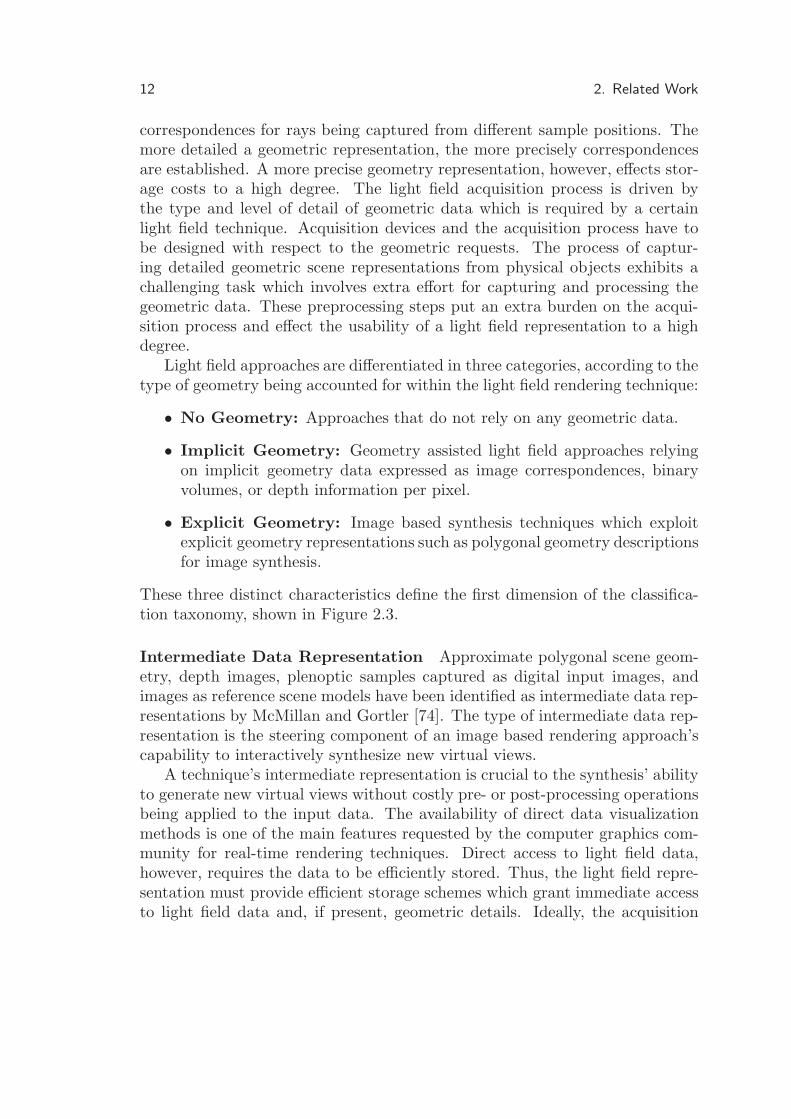
Data RepresentationWithout any geometric data being integrated, the complete light field samplingcan be regarded as a collection of 2D digital images which are accessible di-rectly without the need for further data processing. Note, however, that forlight field samples being acquired from physical objects using digital cameradevices, only these parts of the input images contribute to the final image baselight field sample representation which cover the area of the opposing imageplane representation.SynthesisLight field synthesis is performed on a per-pixel basis by interpolating the lightfield samples of adjacent sample positions. For each virtual viewing ray beingdefined by its intersection with the two planes L(s, t, u, v) adjacent sample po-sitions are identified from the camera plane intersection at coordinates (s, t).To determine the final color, light field sampling data is extracted and inter-polated for the image plane intersection point at (u, v) for each of the adjacentsample positions (see Figure 2.4, left). Here, quadralinear interpolation gener-ates virtual views with only a few aliasing artifacts, whereas nearest neighborand linear interpolation result in noticeable artifacts (see Figure 2.5).
The overall visual quality, however, is effected by the amount and densityof light field samples being available for view interpolation. With the increaseof samples, the rendering quality enhances whilst the storage efficiency suffersfrom dense sampling patterns. The rendering performance of this direct inter-polation scheme based on per-ray interpolation is limited by the virtual view’starget resolution as a ray is being evaluated for each target pixel.
Using texture mapping techniques the interpolation can be implemented
2.5. Survey of Light Field Rendering Approaches 17
(d)(a) (b) (c)
Figure 2.5: The effects of interpolation on ray synthesis. a: Light field rendering ofthe Happy Buddha model with quadralinear interpolation. b: Closeup rendered with nointerpolation. c: Linear interpolation on the (s, t) plane. d: Quadralinear interpolation in(s, t, u, v). All images courtesy of Levoy and Hanrahan [63].
more efficiently [105, 123]. For this rendering approach a polygonal represen-tation of the camera plane quadrilateral is drawn with the virtual viewpoint’sviewing transformation being applied. The quadrilateral is defined by multiplefetches such that a single fetch (F (C0, C1, C2, C3)) is defined by four samplepositions on the camera plane Cn = (sn, tn); n = [0, 3]. For each fetch, texturecoordinates Tn = (un, vn); n = [0, 3] are determined by intersecting the raysfrom the virtual viewpoint through the sample positions with the image plane.The texture coordinates are then being applied to map the image representa-tion of a light field sample to the rendered camera plane fetches (see Figure 2.4,right).
While increased rendering performance is achieved using the fetch basedinterpolation technique, image synthesis quality suffers. Visible seams are vis-ible at the fetch boundaries. If overlapping fetches are rendered and blendedtowards the edges, partial synthesized views are smoothly blended and thus,noticeable visible edges in the final composed image are avoided. At the bor-ders of the fetches, however, the blending results in slightly ghosting artifactsdue to incoherent visual information being blended in these regions.
Although full 6 DOF are available for virtual viewpoint selection, the virtualviewing position is limited to lie within a viewing cone, defined by the size andthe arrangement of the camera- and the image plane. Thus, it takes multiplelight slabs to represent all possible views of an object. Therefore line spacemay be tiled using a collection of light slabs.
It has been shown that light field rendering as described above will providesatisfactory rendering results, if the observed object is positioned exactly onthe image plane. In the general case, noticeable ghosting artifacts will appear

18 2. Related Work
Ci Ci+1Ci-1
Image Plane
Camera Plane
Pcami+1
Pobj
Pcami
Image Plane
Camera Plane
Pobj
Ci Ci+1Ci-1
Figure 2.6: Depth correction of rays. Without depth correction, the intersection pointsobserved from adjacent cameras do not necessarily correspond to an identical surfacepoint. With depth correction, camera rays passing through a common surface point areused for interpolation.
due to incoherent light field information for adjacent rays. Such incoherencyis due to rays hitting the object at a surface point far from the image plane,resulting in deviating intersection points on the image plane (see Figure 2.6,left).AcquisitionFor the acquisition of light field samples a variety of acquisition devices is ap-plicable. Gantries as well as camera arrays can be used to acquire two planelight fields. With multi-lense and multi-camera setups dynamic light fields areacquirable.CategorizationThe two plane light field rendering technique represents a light field approachwhich implements image synthesis based on previously acquired samples of theplenoptic function without the need for additional geometric data. It providesa uniform sampling pattern which is invariant in translations but shows varia-tions in the directional domain. Using state-of-the-art acquisition techniques,light field samples can be exploited for image synthesis directly without furtherprocessing.
2.5.2 The Lumigraph
The Lumigraph approach samples the plenoptic function along a cubic surfacearound an object of interest [35]. It provides all information that is neededto simulate the light transfer from one region of space on the surface of thecubic setup to all other regions [65]. This cubic representation of the plenoptic

2.5. Survey of Light Field Rendering Approaches 19
function is equivalent to a representation defined by six light slabs as proposedby Levoy and Hanrahan [63]. It allows to synthesize virtual views with full 6DOF without any constraints concerning the positions and orientation of thevirtual viewpoint, as long as it is chosen to lie outside the region bounded bythe six light slabs.ParametrizationAs the lumigraph representation is built from six two plane setups. Conse-quently, the uniformity characteristics of the two plane approach also applyfor the combination of six light slabs. Thus, the lumigraph setup does provideuniformly distributed sample positions on the surface of cubic bounding vol-ume around an object, but does exhibit non uniform sampling of directions, asthe solid angle covered by a single pixel within an image representation variessignificantly over the overall image.Geometric RepresentationGortler et al. have shown that, while improving the quality of radiance inter-polation, the amount of input samples can significantly be reduced if geometricinformation about the scene is taken into account to identify ray correspon-dences. The geometric information can take the form of a coarse trianglemesh, a binary volume [16], or per-pixel depth information [96,124]. However,Gortler et al. suggest storing an explicit polygonal approximation of the ob-served object.Data RepresentationAs the geometric data is essential for the lumigraph rendering approach, ge-ometry processing is indispensable for image synthesis. While the light fieldsamples are stored according to the two plane light field approach, the explicitgeometric 3D model is processed and stored independently. In practice, the ge-ometric model is processed prior to the image synthesis process in a separatedtask.SynthesisTo avoid ghosting artifacts which result from incoherent light field samplesbeing interpolated, the geometric scene representation is exploited to ensurerays consistency. Without the object’s geometry being considered, a virtualviewing ray is reconstructed from sample rays which intersect the image planeat the same position. These sample rays, however, are likely to intersect theobject at different positions and thus, represent incoherent light field data (seeFigure 2.6, left).
With additional geometric information about the observed object beingavailable, the ray-object intersection point PObj can be determined for a rayL(s, t, u, v). Then, for the ray L and a given Ci(si, ti) one can compute cor-responding I ′(u′, v′) for a ray L′(si, ti, u
′, v′) that intersects the object at the
20 2. Related Work
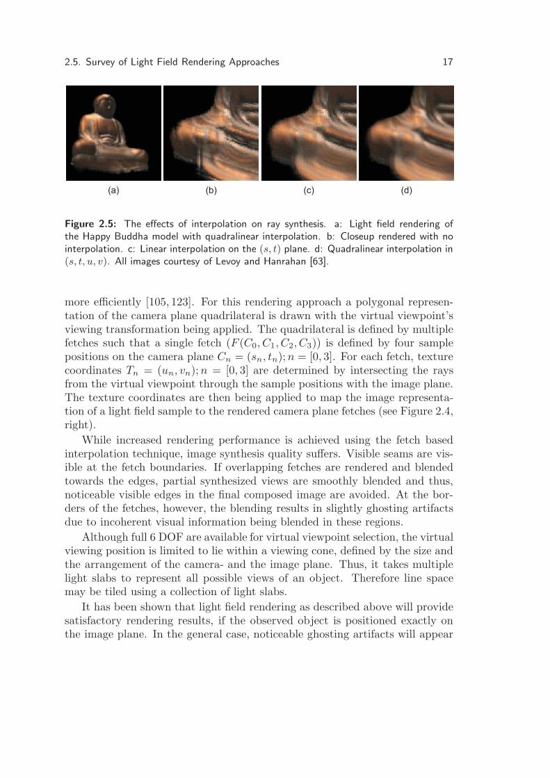
Figure 2.7: Lumigraph rendering results of a stomach data set. Left: View synthesiswithout depth correction of rays. Right: Rendering results with depth correction of raysbeing applied for image synthesis based on depth maps. Image courtesy of Vogelgsangand Greiner [124]
same surface point PObj (see Figure 2.6, right).
Improved rendering results showing less ghosting artifacts for the same (s, t)sample resolution are observed with the depth correction being applied (seeFigure 2.7). The effectiveness of the depth correction of rays is dependent onthe geometry’s level of detail. On the one hand, more precise geometry rep-resentations result in improved depth correction. On the other hand, complexraytracing techniques are to be applied to establish ray-object intersections fordetailed geometry representations and storage cost are effected by the geome-try’s precision to a high degree. Rendering efficiency can be improved if fetchbased rendering approaches are applied to the lumigraph representation, com-parable to the fetch based technique described in Section 2.5.1. In contrast tothe straight forward lumigraph rendering approach the fetch based approach’sperformance is not effected by the target resolution but the amount of fetchesbeing drawn [20, 106]. Notice that disparity artifacts [16] occur for situationsin which the virtual view spans over a boundary edge of the cubical setup.In these situations the non uniform sampling of direction becomes visible andappears as visible discontinuities along the edge.AcquisitionGortler et al. suggest storing a rough polygonal approximation of the observedobject in order to allow for depth corrections. To recover a geometric modelof the scene, however, additional effort has to be spent. 3D scanning tech-nology [95] as well as sophisticated stereo vision [93] and image based feature

2.5. Survey of Light Field Rendering Approaches 21
extraction methods [8, 24] are applied to extract the geometric representation.Light field samples can be acquired similar to the two plane representationdescribed in Section 2.5.1.
For flexibility reasons Gortler et al. have presented an acquisition approachwhich accept input images from arbitrary placed cameras. If a geometric scenerepresentation is available prior to light field sampling and intrinsic as well asextrinsic camera parameters can be evaluated for each input image, an inputimage can be projected onto the geometry and re-projected into the pre-definedsample position. This technique, known as rebinning [61], then allows to gen-erate a lumigraph representation using commodity imaging devices.CategorizationThe lumigraph representation implements a uniform sampling of the plenopticfunction which is invariant in translations, but exhibits non uniform samplingof directions. Explicit geometric representations are utilized for depth correc-tion of rays to optimize rendering quality and reducing sampling complexity.The geometry representation, however, is extracted and processed in a separatetask. Thus, image synthesis cannot be performed without the geometry beingprocessed in advance.
2.5.3 Spherical Light Field Rendering
Spherical light field rendering techniques overcome the problem of disconti-nuities observed with multi light slab setups by parameterizing rays using aspherical representation. The use of spherical parametrization schemes pro-vides a symmetric representation of the complete flow of light, which allows forhandling arbitrary viewpoints and directions [47]. Several flavors of sphericalparameterizations have been published in the past under various names. Allof these approaches define the bounding volume around an object of interestto be a spherical volume. Commonly they implement a parametrization whichdefine sample positions to be equally distributed on the surface of the bound-ing sphere. The parametrization of direction, the representation of individuallight field samples, as well as the rendering process, however, differ significantlybetween approaches. This section discusses different spherical representations.
Spherical Light Fields Spherical light fields have been introduced to thecomputer graphics community by Ihm et al. in 1997 [47]. Spherical light fieldsdefine a representation scheme that is based on two spheres. Sample positionsare defined by uniformly distributed discrete surface points on the first, thecamera sphere. For each of the sample positions, a second, so called directionalsphere, is utilized to parameterize the directional domain for a certain sampleposition. Using these two spheres, a ray is defined by its intersection with both

22 2. Related Work
of these spheres (see Figure 2.8, left).ParametrizationSample positions are defined on the surface of the camera sphere using a lon-gitudinal parameter (θp) and a latitude parameter (φp). Discrete values of(θp, φp) are applied to formalize sample positions on the camera sphere’s sur-face. Discrete directions are defined using the directional variables (θd, φd) todefine surface points on the directional sphere. The directional sphere is posi-tioned tangential to the sample position. Thus, a ray passing through a sampleposition is explicitly defined by the sample positions and its intersection withthe directional sphere (L(θp, φp, θd, φd)).
As L can be expressed as a combination of two functionsL(θp, φp, θd, φd) = fd(θd, φd) = (fp(θp, φp))(θd, φd), the task of samplingthe 4D spherical light fields is reduced to the finite approximations of twospheres. Discretization of both, the positional and the directional sphere, isinitialized based on an octahedron, where each triangle face corresponds to theeight regular patches on the sphere. Each triangular face is then successivelysubdivided into four finer triangles. Following this approach arbitrary finediscretizations of the positional- and the directional sphere are achieved. Forthe positional sphere, each of the vertices of the polyhedron represents adiscrete sample position. On the directional sphere, the values of a plenopticsample is associated with the barycentric center of a triangular face. Foreffective storage, the discrete samples are recorded into a two dimensionalarray. The subdivision process guarantees the parametrization to be invariantin position and direction, thus providing a uniform parametrization of bothdomains.Geometric RepresentationThe two sphere representation does not integrate any geometric details aboutthe scene.Data RepresentationIn practice, up to 65K vertices are generated for the positional sphere anda level 5 subdivision is applied to discretize the directional sphere. With24 bit color coding this results in about 1.5 GB data storage. The uniformrepresentation, however, allows wavelet compression schemes to be appliedto the image data [25, 100, 136]. With wavelet compression being applied acompression ratio of up to 22.4 : 1 has been achieved by Ihm et al. [47].
SynthesisLight field synthesis is performed using a raycasting approach based on thespherical representation by rendering the smooth shaded triangles of thepositional polyhedron. For each vertex a ray is casted from the virtual viewing

2.5. Survey of Light Field Rendering Approaches 23
position through the vertex position. From the intersection of this ray with thedirectional sphere, which is associated with the current vertex, the plenopticsample is resampled using neearest neighbor interpolation techniques. Theinterpolation result is applied as vertex color to the current vertex. For thefinal result, per-pixel color values within the triangles are interpolated basedon barycentric weights form the vertex colors.
The quality of this rendering approach is limited by both, the chosen reso-lution of the directional sphere, as it defines the sample image resolution, andthe subdivision level chosen to parameterize the positional sphere. Reducingthe amount of sample positions will result in visual details not being sampledand additional loss in image synthesis quality due to interpolation techniquesbeing applied to relatively large triangles. Without the actual scene geometrybeing taken into account, ghosting artifacts appear for sparsely sampled lightfields [47].AcquisitionWith up to 65K positions being used in practice, this spherical approach issuited for artificial light fields to be generated from synthetic data. The acqui-sition of physical objects, however, is a challenging task. Spherical light fieldsas proposed above have not been acquired in the past. Nevertheless, sphericalgantries as described in Section 2.3 could be utilized to acquire such type oflight field.CategorizationThe spherical light field parametrization represents a uniform sampling of posi-tion and direction. Image synthesis is performed directly on the input sampleswithout any pre- or post-processing being applied to the input data. With adense sampling of position and direction, good rendering results are achievableat high storage costs but without geometric assistance.
Two Sphere Parametrization The two sphere parametrization implementsa spherical parametrization of sample position and direction using two identicaluniform spherical representations. Both of these are defined as the sphericalbounding volume of a scene which is to be captured. The two sphere repre-sentation was first introduced to the computer graphics community in 1998 byCamahort et al. [16].ParametrizationThe spherical representation chosen for position and direction is akin to theone chosen by Ihm et al. [47] to parameterize camera space as described in theprevious paragraph. Discrete sample positions are achieved by subdividing aspherical approximation based on a polyhedra which provides the most popu-lar subdivision of the unit sphere [30]. However, Camahort et al. construct a

24 2. Related Work
Spherical Sphere - Sphere Sphere - Plane
Figure 2.8: Left: Spherical Light Fields use intersection with a positional sphere (largecircle) and directional sphere (small circle). Middle: Two-Sphere parameters are deter-mined by intersecting the same sphere twice. Right: Sphere-Plane coordinates consist ofthe intersection with a plane, and the normal direction of the plane.
special polyhedral generator by initially subdividing the 20 faces of an icosa-hedron. The generator being used for the subdivision process then provides60 identical faces. By successively applying the subdivision process L times,4L×60 faces are generated. In practice, L = 5 or L = 6 yielding 61K and 245Kfaces are chosen to create a spherical parametrization for position and direc-tion. Usually, both parameterizations are chosen to be of the same granularity(see Figure 2.8, middle).
In contrast to the camera space parametrization presented by Ihm et al.,Camahort et al. define discrete sample positions as well as sample directionsto be represented by the barycentric center of the triangular fetches.Geometric RepresentationNo geometric information is being represented in the two sphere light field rep-resentation.Data RepresentationThe huge amount of sample positions and -directions effects storage efficiency toa high degree. Assuming a 24bit RGB color scheme, a total of N ×N ×3Bytesis consumed (with N being the patch count). Thus, a total of approximately10.4 GByte of memory is consumed to store a 61K parametrization. Withspherical wavelets [99] being applied, storage costs can be significantly reducedby a compression ration of up to 60:1.SynthesisLight field synthesis is implemented using a ground truth ray tracing ap-proach [33]. For each synthesized ray, the intersection points of the ray andthe unit sphere are computed. In a second step the two intersected patches

2.5. Survey of Light Field Rendering Approaches 25
of the positional and the directional sphere are identified. As the barycentriccenters of the patches define discrete sample positions on the positional sphereand represent discrete plenoptic samples on the directional spehere, the finalpixel color value is computed efficiently using nearest neighbor interpolationschemes. Rendering performance is thus proportional to the desired image size.In comparison to light field rendering introduced by Levoy and Hanrahan, thisrendering approach takes up to three times longer than rendering a single lightslab [16]. The two sphere rendering approach, however, achieves improved ren-dering quality compared to Levoy’s and Hanrahan’s approach. Discontinuityartifacts which are observed at light slab boundaries for surround light fields asimplemented for the lumigraph by Gortler et al. do not appear. However, im-proved rendering quality comes at the price of densely sampled light fields andthus increased data volume. Best rendering quality is achieved for sphericalparameterizations yielding 20K and above sample positions (see Figure 2.9).AcquisitionFor synthetic scenes, two sphere light field representations are built using aray tracer which can be instructed to shoot individual rays, joining pairs ofpoints on the sphere to determine the light transport between two fetches. Theacquisition of physical objects has not been in focus of Camhort et al.’s work.It could, however, theoretically be implemented using spherical gantries anddigital imaging devices.CategorizationThe two sphere parametrization of light fields yields a light field approach thatis capable of producing high-quality virtual views from densely sampled lightfields without the need for geometric data for depth correction of rays. Theuniform sampling of direction and position abet constant rendering quality forthe overall surrounding of the scene.
Sphere - Plane Parametrization The sphere plane parametrization wasintroduced by Camahort et al. [16] as an alternative approach to the two spherelight field representation. Thus, the sphere plane parametrization adopt someof the parametrization issues being introduced with the two sphere approach(see Figure 2.8, right).ParametrizationDiscrete sample positions on the spherical surface of the convex hull aroundan object are determined by subdividing an icosahedron. Each barycentriccenter of a triangular fetch then represents a sample position. A planar imageis associated with every sample position. The planar image represents a lightfield sample for a discrete position. The associated image is generated byparallel projection along the inward looking normal direction of the triangular

26 2. Related Work
Figure 2.9: Rendering results of the two sphere light field rendering approach. Lightfield rendered from a two sphere light field sampled at a sample resolution of 65K samplepositions. Image courtesy of Camahort et al. [16].
fetch which defines the concrete sample position. The image plane is definedto be oriented orthogonal to the fetch normal and positioned at the center ofthe unit sphere. For each defined sample position a parallel projection of thesynthetic scene is stored. Additionally, depth maps storing per-pixel distancesare stored with each light field sample. The depth map captures orthogonalsigned distances of the visible object surface to the image plane on a per-pixelbasis.
While the sample positions are uniformly distributed on the surface of thespherical bounding volume, a uniform sampling pattern is not applied to rep-resent the radiance along rays. Only rays with directions parallel to the inwardlooking normal of a sample position are captured. Considering the image rep-resentation of this parallel projection and the solid angle being covered byindividual pixels, it can be shown that the solid angle varies significantly be-tween pixels for the overall image. Thus, this sphere plane representation doesnot provide a uniform parametrization for the directional domain.Geometric RepresentationLight field samples and depth images are stored as separate textures. Whilethe RGB representation of the captured scene is stored in the light field images,the depth images store an implicit geometric scene representation as orthogonaldistances of the object’s surface to the image plane.Data RepresentationWith two textures being stored for each sample position, the data volume iseffected by the amount of sample positions and the sampled image resolutionto a high degree. In practice, thousands of light field samples are utilized torepresent a complete light field. However, a compression ration of up to 60:1

2.5. Survey of Light Field Rendering Approaches 27
is achieved with JPEG [84] compression techniques being applied to the im-age data and Lempel-Ziv [138] compression schemes being applied to the depthmap. Then, a light field sampled from 20K positions at a resolution of 256×256is roughly about 170 MBytes, including the depth maps.SynthesisLight field rendering is implemented based on texture mapping techniques.Each sample image is assigned as texture to the vertices of the triangular fetchfrom which’s barycentric center it has been captured. Within the light fieldsynthesis the vertices of each triangle fetch are projected onto the fetch’s imageplane to determine each vertex’s texture coordinates, using the virtual view-point as center of projection. The texture samples of vertices being sharedby adjacent fetches will in the general case provide incoherent visual informa-tion as adjacent samples represent orthogonal projections with varying centralviewing direction. Thus, this incoherence is exposed as visual seams at thetriangular edges of the spherical approximation (see Figure 2.10, left). Apply-ing texture blending on overlapping fetches, the visual discontinuity of sharpedges is omitted at the price of slightly blurring artifacts in these regions (seeFigure 2.10, right).
With the available depth map being exploited for depth correction of rays,visible seams and ghosting artifacts are reduced to a reasonable amount (seeFigure 2.10, bottom row). For depth correction of rays the depth imageis traced to establish a ray-object intersection for three vertices of a singlefetch [127, 128]. If the disparity of the determined depth values, however,exceeds a pre-defined threshold the fetch is subdivided at rendering time toaccount for geometric details of the captured object. This subdivision processis iteratively repeated, until a predefined minimal fetch size is achieved or thedepth disparity does not further exceed the given threshold. In the worst case,the subdivision is repeated until the fetch size narrows down to the size of asingle pixel.
The subdivision process is driven by the current viewing parameters. Thus,the final topology of the triangle mesh being used for image synthesis varieswith changing virtual viewpoints. As a consequence, moving the viewpointaround will lead to noticeable artifacts resulting from topology changes. Theoverall rendering quality of the sphere plane light field approach is dependenton both, the resolution of the depth map and the resolution of the images. Incontrast to the two sphere light field rendering approach the performance isnot limited by the target resolution but by the amount of sample positions.AcquisitionAs stated by Camahort et al. this representation is especially suited to gener-ate light field representations from complex synthetic scenes. Although being

28 2. Related Work
Figure 2.10: Rendering results of the sphere plane light field rendering approach. Toprow: Light field synthesized from a dataset containing 1280 sample images at 256 × 256pixel resolution. The left image was rendered without blending being applied to fetches.Notice the seams at the fetch boundaries. The right image shows rendering results withblending being applied. Notice the ghosting artifacts a the boundaries of the fetches.Bottom row: Light field of the Stanford Bunny, rendered from a light field containing20480 samples each at a resolution of 256×256 pixel with depth correction of rays (Left:Without blending, Right: With blending) Image courtesy of Camahort et al. [16].
theoretically possible, physical objects have not been acquired in the past. Forsynthetic scenes the images are generated with any standard rendering engineby adjusting the view settings and rendering the scene with parallel projectionfrom the desired sample position. Depth maps are easily generated by extract-ing the z-Buffer depth information and evaluating the distance to the imageplane.CategorizationThe uniform representation of sample positions being utilized in this approachallows to continuously synthesize arbitrary views from any position around theobject. However, the parallel projection being associated with each sampleposition does not provide a uniform sampling of directions. With the depthcorrection of rays being applied based on the implicit geometry representation

2.5. Survey of Light Field Rendering Approaches 29
the structure of the spherical approximation is adjusted according to the inputdata’s depth complexity at rendering time. The depth information stored in thedepth maps of adjacent fetches steer the subdivision process at run-time. Thus,the final appearance of the subdivided spherical proxy can first be establishedwith all of the depth maps being available.
2.5.4 Unstructured Light Fields
In the past, two major contributions in the field of unstructured light field ren-dering have been published. Both approaches implement a light field renderingtechnique which does not require a predefined setup of sample positions andassociated input images to synthesize new virtual views. However, both ap-proaches implement different sample representation and image synthesis tech-niques.
Unstructured Lumigraph Rendering The basic idea of Unstructured Lu-migraph Rendering is to implement a geometry assisted light field renderingtechnique that accepts input images from cameras in general positions whichare not restricted to a plane or to any specific manifold. It should, however,be general enough to also implement special setups such as the two planeparametrization, a cubic arrangement of light slabs or any sort of sphericalparametrization [13]. The work on unstructured lumigraphs has been inspiredby View Dependent Texture Mapping techniques [22, 23, 87] which apply pro-jective texture mapping for efficient real-time image synthesis [39]. It picksup recent enhancements and extensions to the basic light field rendering tech-niques, for rendering digitized three-dimensional models in combination withacquired images [89, 103,131].ParametrizationUnstructured lumigraphs define the sample positions to be free of any restric-tions in position or orientation as long as they are chosen to lie outside theconvex hull of the object of interest. As the sample positions are to be chosenfreely without any given constraints on the sample arrangement, uniformitycannot be guaranteed in the general case. If, however, an acquisition devicelike a gantry is used to acquire light field samples from predefined positions,according to the spherical parametrization, uniformity can be achieved. Then,of course, the benefit of flexible acquisition process is lost.Geometric RepresentationIn addition to the light field samples acquired from arbitrary sample positionsan explicit polygonal approximation of the scene is to be generated and storedwith the set of input images. Typically the polygonal representation is gener-ated in separate task independent of the light field acquisition process. Buehler
30 2. Related Work
C1
C2
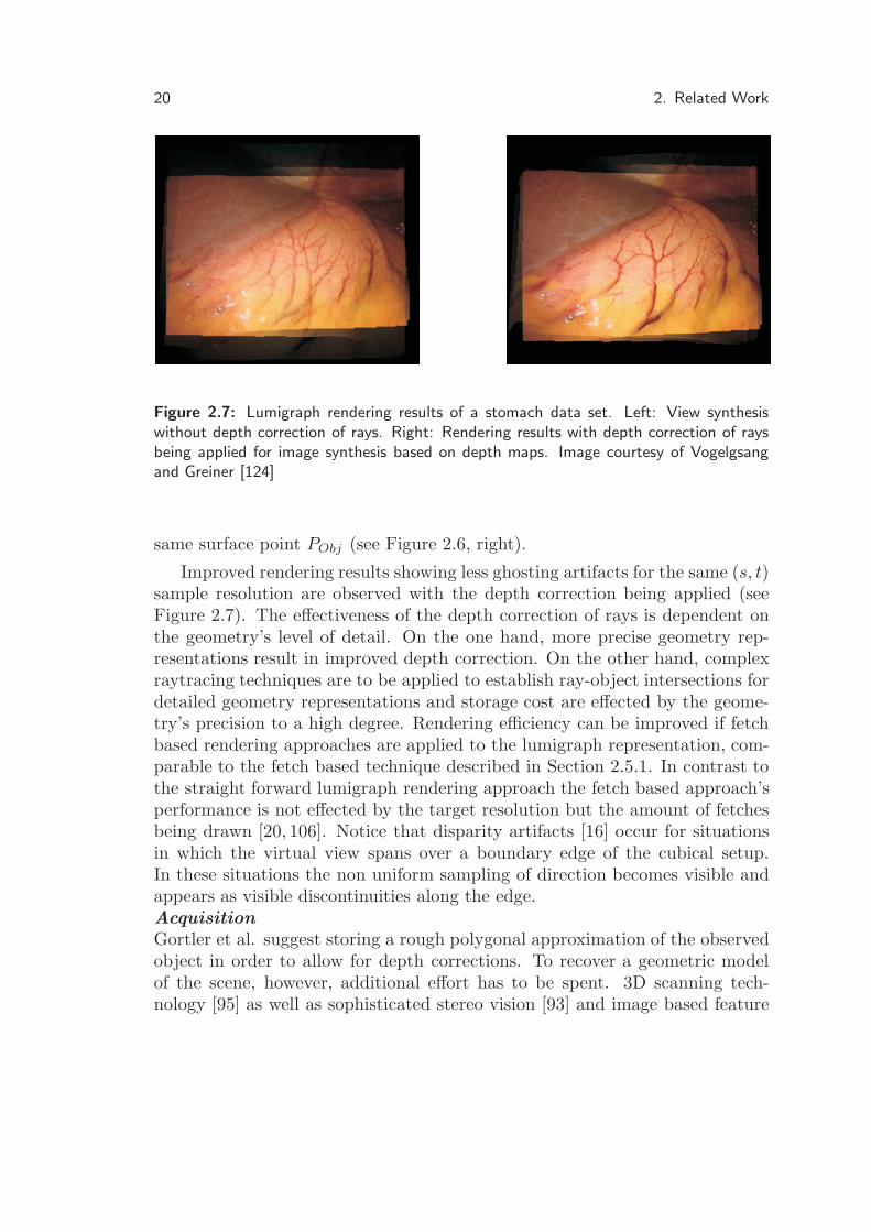
Figure 2.11: Top: Triangulation of the image plane. Bottom Left: Camera blending field.Bottom Right: Rendering results of ”Hallway” data set based on the camera blendingfield. Image courtesy of Buehler et al. [13].
et al. [13] have declared an explicit geometry approximation of the scene to bebest suited for unstructured lumigraph rendering.Data RepresentationLight field synthesis is dependent on the knowledge of sample positions andimaging parameters. As these are not defined for the unstructured parametriza-tion a priori, internal projection parameters as well as external transforma-tion parameters are to be stored with every sample being acquired. With theamount of sample positions not being defined a priori, assumptions on thememory consumption cannot be made. As a rule of thumb, less samples haveto be acquired if a precise geometric representation is available. The granular-ity of the geometry proxy, however, effects the storage costs to a high degree.SynthesisFor a virtual view to be synthesized from the input images, the positions ofthe source cameras’ centers are projected into the desired virtual image plane.The projected vertices are then being triangulated and used to reconstruct

2.5. Survey of Light Field Rendering Approaches 31
the interior pixels, according to Heigl et al. [42]. The unstructured lumigraphrendering approach calculates a camera blending field for the desired imageplane in a first step and applies projective texture mapping techniques in asecond step to synthesize a virtual view. A pixel’s blending weight represents asample camera’s contribution to the pixel’s final color. The blending weight iscalculated with respect to a virtual viewing ray through an image plane pixelrp. The weight is determined from the angular distance of rp to the samplecamera’s central view direction, the sample camera’s distance to the observedobject, and the sample camera’s field of view (FOV). A sample camera’s weightis reduced with rising angular distances, increasing distance to the object andwith the specific pixel being observed in boundary regions of the FOV.
To efficiently compute the blending field for a certain image plane the blend-ing weight is determined at a set of discrete points on the image plane, only.The discrete points are then triangulated over the image plane and the blend-ing weights are being interpolated. The triangulation of the image plane isperformed by projecting the edges of the polygonal proxy to the image plane.All edge-edge crossings are inserted as vertices in the image plane. Addition-ally, all sample camera positions are projected to the image plane and insertedas vertices. Finally, a dense regular grid of vertices is included on the desiredimage plane [13]. A constrained Delaunay triangulation is then applied to thevertices of the image plane [101]. For each vertex a set of cameras and theirassociated blending weights are stored (see Figure 2.11, top and bottom left).
The final image is rendered as a set of projectively mapped triangles. Eachtriangle is rendered multiple times according to the different sample camerasassociated with each of the triangle’s vertices and their different textures beingmapped to the triangle fetch. Multiple renderings of the same fetch are finallycomposed by alpha blending according to per-pixel blending weights from theblending field. Since each polygon is treated independently, smooth transitionacross polygon edges is not guaranteed. This rendering approach provides so-phisticated rendering results for detailed polygonal approximations only. Withonly a sparse geometric approximation being available, ghosting artifacts be-come visible in the synthesized image (see Figure 2.11, bottom right).AcquisitionThe acquisition of detailed geometric representations, is a major burden on theacquisition process. For the acquisition of real objects, complex 3D geometryextraction methods are to be employed to generate detailed models of the cap-tured scene. While commodity camera equipment can be used to capture lightfield samples from arbitrary positions, extra effort has to be spent to capturethe scene’s geometry. For this reason, only very simplified versions of the ge-ometry are used for image synthesis. In practice geometry representations like

32 2. Related Work
boxes or planes are used to represent a captured scene [13]. This simplificationcomes at the price of visible ghosting artifacts in the final image. If not a verysimple representation is chosen, but a detailed model is used instead, complexgeometric processing techniques are to be applied prior to the image synthesisprocess in a separated task to make the geometric representation available.CategorizationUnstructured lumigraph rendering provides a flexible light field rendering tech-nique that may be used to provide uniformly sampled light fields. But the aimof this approach is targeted at the free-hand acquisition of light fields. For thisgeneral case uniformity cannot be guaranteed. The explicit geometric repre-sentation of the scene effects all aspects of this light field synthesis approach.Rendering quality is improved by applying detailed geometric representations,whilst it effects pre-processing and storage costs to a high degree.
Free Form Light Field Rendering Free Form Light Field Rendering waspublished by Schirmacher et al. [97] as an alternative light field rendering ap-proach to unstructured lumigraph rendering. With this approach, however,the optical centers of the sample cameras are considered to lie on a commonarbitrary free form surface, while the camera position and orientation can bechosen freely [97].ParametrizationThe free form surface is defined by a convex triangulated polygonal mesh, alsocalled the camera mesh. The camera mesh is built from the sample positions,each defining a vertex of the polygonal mesh. For each camera position an in-dividual image plane is defined. Thus, the camera space is defined globally bythe camera mesh, while the image space is defined separately on a per camerabasis by their image planes. Each ray passing through the bounding volumeof the observed object can then be defined by the intersection with the cameramesh and the image plane of the associated camera. To ensure each viewingray to be reconstructible, each camera is to be placed such that the completesilhouette of the observed object is captured. Under this restriction, arbitraryviewing rays passing through the convex hull do always intersect the cameramesh and at least one camera image plane (see Figure 2.12, left). However,uniformity in position and direction cannot be guaranteed, as the sample po-sitions and their orientation is not pre-defined in a uniform manner.Geometric RepresentationThe free form light field approach exploits geometric scene details for depthcorrection of rays. The technique can operate on a variety of geometric repre-sentations, such a explicit polygonal representation [35], binary volumes [16],or depth maps [125].

2.5. Survey of Light Field Rendering Approaches 33
Data RepresentationLight field samples are stored separately from the geometric representation.For each light field sample the camera parameters, namely camera transforma-tion and intrinsic camera projection parameters have to be stored in addition.With the camera arrangement to be chosen freely to lie anywhere outside theconvex hull of the observed scene, uniformity in position and direction cannotbe guaranteed, as well as storage costs are not determinable in advance. Thus,while the free form parametrization opens up for a flexible light field represen-tation, rendering quality cannot be guaranteed. Without a uniform samplingscheme being essential part of this representation, rendering artifacts resultingfrom varying sampling resolution and sample position density are likely to ap-pear within the light field synthesis.SynthesisImage synthesis is implemented by rendering the front faces of the texturedpolygonal camera mesh. Each triangle fetch of the camera mesh is texturedaccording to the input images of the three corresponding cameras which definethe vertices of the current triangle. To obtain a triangle’s final appearance, itsprojection onto each of the three camera image planes is rendered separatelyand alpha blended. If we assume the triangle to be defined by the verticesV0, V1, V2, the triangle is projected to the image plane corresponding to V0
first, with an alpha value of 1 assigned to V0, alpha value 0 assigned to V1, V2,and the alpha values being linearly interpolated over the triangle. With thisprocedure being applied accordingly to V1 and V2 the resulting three samplesare interpolated using the assigned alpha values for the final appearance of thetriangle.
If the sampling density is not high enough, this approach leads to seriousblurring and ghosting artifacts. With depth correction being applied, theseartifacts can be compensated to some degree. With an approximation of thegeometry to be known, a ray-object intersection can be determined for each rayemerging from a virtual viewpoint and passing through a vertex. With depthinformation being available on a per-vertex basis, the vertices of a triangle arethen projected onto the approximate geometry surface. An additional depthis estimated for the triangle’s center. If the overall depth disparity of the fourdepth estimations within a triangle exceeds a certain threshold, the triangle issubdivided. This depth estimation and subdivision procedure is repeated untilthe depth threshold or a minimum triangle size is reached (see Figure 2.12,middle). The minimum triangle size is specified by the target image resolution.Thus, subdivision is repeated recursively until a minimum triangle size of onepixel is reached in the worst case.
With the depth correction being applied to four discrete positions of a

34 2. Related Work
C1 C2
C3
I1I2
I3
M
Figure 2.12: Left: Camera Mesh M built from input camera positions Cn, displayingimage planes In associated with each camera. A viewing ray is defined by the intersectionwith the camera mesh and the image plane. Middle: Refined camera mesh utilized todetermine camera blending weights with depth correction being applied. Right: Renderingresults of light field containing 107 input samples with depth correction being applied.Image courtesy of Schirmacher et al. [97].
triangle, only, high-frequency changes between these depth samples are notaccounted for by the depth correction, leading to ghosting artifacts in the finalimage (see Figure 2.12, right).
The depth correction being applied to the camera mesh results in improvedrendering quality. Rendering quality, however, comes at the cost of a perfor-mance drop caused by the recursive subdivision process. As the subdivisionis steered by per-vertex depth values, which are in turn determined along theray from the current viewpoint, the topology of the subdivided mesh varieswith changing viewpoints. This inconsistent reconstruction of viewing rays isalso observed for unstructured lumigraph rendering [13]. While moving thevirtual viewpoint around the object, the inconsistence may lead to noticeableartifacts. With the subdivision process being applied to the complete cameramesh at run-time, rendering is performed solely after the acquisition processhas been completed.
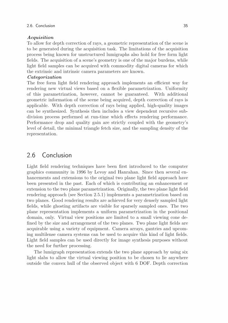
2.6. Conclusion 35
AcquisitionTo allow for depth correction of rays, a geometric representation of the scene isto be generated during the acquisition task. The limitations of the acquisitionprocess being known for unstructured lumigraphs also hold for free form lightfields. The acquisition of a scene’s geometry is one of the major burdens, whilelight field samples can be acquired with commodity digital cameras for whichthe extrinsic and intrinsic camera parameters are known.CategorizationThe free form light field rendering approach implements an efficient way forrendering new virtual views based on a flexible parametrization. Uniformityof this parametrization, however, cannot be guaranteed. With additionalgeometric information of the scene being acquired, depth correction of rays isapplicable. With depth correction of rays being applied, high-quality imagescan be synthesized. Synthesis then includes a view dependent recursive sub-division process performed at run-time which effects rendering performance.Performance drop and quality gain are strictly coupled with the geometry’slevel of detail, the minimal triangle fetch size, and the sampling density of therepresentation.
2.6 Conclusion
Light field rendering techniques have been first introduced to the computergraphics community in 1996 by Levoy and Hanrahan. Since then several en-hancements and extensions to the original two plane light field approach havebeen presented in the past. Each of which is contributing an enhancement orextension to the two plane parametrization. Originally, the two plane light fieldrendering approach (see Section 2.5.1) implements a parametrization based ontwo planes. Good rendering results are achieved for very densely sampled lightfields, while ghosting artifacts are visible for sparsely sampled ones. The twoplane representation implements a uniform parametrization in the positionaldomain, only. Virtual view positions are limited to a small viewing cone de-fined by the size and arrangement of the two planes. Two plane light fields areacquirable using a variety of equipment. Camera arrays, gantries and upcom-ing multilense camera systems can be used to acquire this kind of light fields.Light field samples can be used directly for image synthesis purposes withoutthe need for further processing.
The lumigraph representation extends the two plane approach by using sixlight slabs to allow the virtual viewing position to be chosen to lie anywhereoutside the convex hull of the observed object with 6 DOF. Depth correction

36 2. Related Work
of rays is implemented based on a sparse geometric approximation of the sceneto reduce ghosting artifacts. However, lumigraph rendering shows noticeabledisparity artifacts at the boundaries of two adjacent light slabs. This effect isdirectly related to the non uniform sampling of directions which becomes visibleas artifacts in these regions. While the light field samples can be acquiredaccording to the two plane approach, effort has to be spent on the acquisitionof the geometric scene representation. As the geometry is fundamental to thelumigraph rendering technique, it is to processed prior to the rendering task ina separate task. Thus, samples being acquired during the acquisition processcan be visualized directly, only, if the geometry has already been processedbefore.
Spherical light field techniques overcome the problem of visible discontinu-ities at the boundary regions of two adjacent light slabs by implementing auniform sampling of positions and directions in a spherical parametrization.All of the spherical approaches presented in Section 2.5.3, however, are in needof a dense sample distribution on the spherical alignment in order to synthesizehigh-quality virtual views. With depth correction of rays being applied by thesphere plane parametrization, the amount of samples is drastically reduced.But still, thousands of sample positions are required. Thus, the spherical tech-niques are especially suited to extract light fields from synthetic objects.
Unstructured light field approaches are focused at accepting input samplesfrom cameras in arbitrary positions. With the sample positions being freelychosen during acquisition, it opens up for a flexible acquisition of light fields, ifthe camera’s intrinsic and extrinsic parameters are known. With the grantedflexibility, however, a uniform parametrization cannot be guaranteed for theseapproaches in the general case. Rendering artifacts resulting from varyingsampling density are likely to appear for these approaches. These artifacts areespecially prominent while interactively adjusting the virtual viewing pose asthese approaches are variant under both translation and rotation. As bothapproaches rely on some knowledge about the scene geometry, extra effort isto be spent on the acquisition of geometric details which reduces the benefitof easy to use light field acquisition. Extra equipment has to be utilized andcostly geometry processing has to be performed prior to virtual view synthesis.With depth correction of rays being applied, high quality rendering results canbe achieved for densely sampled light fields.
All of the light field approaches presented in this chapter are capable ofsynthesizing new virtual views from light field representation at high quality.The achievable quality, however, comes at the high price of extremely densesampling patterns, very detailed geometric representations or computationalcostly processing techniques. These issues effect the usability of the presented

2.6. Conclusion 37
TwoPlane
DataRepresentation
GeometryRepresentation
Sampling Uniformity
UniformOrientation
NonUniform
UniformPosition
DirectRendering
Processingon Rendering
Pre-processing
UniformPosition &Orientation
NoGeometry
ExplicitGeometry
ImplicitGeometry
Lumigraph
Spherical
TwoSphere
SpherePlane
UnstructuredLumigraph
FreeformLight Field
Figure 2.13: Light field rendering approaches categorized by the amount of geometryused for depth correction of rays, data representation and sampling uniformity.
approaches to a high degree. Two plane light field rendering provides sophisti-cated rendering results for a restricted region of virtual viewpoints, only, if thelight field is sampled very densely. While reducing the sampling count signifi-cantly and resolving the virtual point restriction, the lumigraph approach is inneed of detailed explicit polygonal geometry to achieve high quality synthesisresults of non constant quality. Overall quality is limited by disparity artifacts.Spherical approaches eliminate these artifacts but demand both, densely sam-pled light fields and detailed geometry to achieve sophisticated quality. Whilethe unstructured light field techniques are aiming at providing a straight for-ward approach for light field acquisition and rendering, these approaches donot provide a uniform parametrization and exhibit visible artifacts resultingfrom topology adjustments within the light field synthesis.
This thesis presents a new spherical light field parametrization which com-bines the benefit of uniformity being implemented by spherical light field tech-niques and the advantage of geometry assistance in order to reduce sampledensity. The proposed approach implements a new technique that is capable

38 2. Related Work
of synthesizing high-quality virtual views from as few as 42 light field samplesbased on an implicit geometric representation of the scene. Thus, the presentedtechnique opens up for the acquisition of spherical light fields from physical ob-jects which is not available for spherical approaches presented in the past. Anew acquisition technique is presented which captures both, a light field sampleand a depth map of the scene in a single exposure and thus opens up for directdata access without the need for costly geometry processing which has beenthe limiting factor for geometry assisted techniques presented in the past.
3
Spherical Light FieldParametrization with
Per-Pixel Depth
This chapter presents a new spherical light field parametrization which pro-vides a uniform sampling pattern. The proposed approach efficiently representscombined light field samples and implicit geometric information in a texturebased storage format.Sample positions are arranged in a spherical setup based on a spherical ap-proximation being derived from the icosahedron as initial representation. Thespherical arrangement of sample positions allows the virtual viewpoint to bechosen with 6 DOF during the light field synthesis process. Light field synthesiscan be performed in absence of discontinuity artifacts which are observed forthe lumigraph approach and those, which potentially occur for unstructuredlight fields for non uniform sampled scenes.
The image space parametrization exploits existing environment mappingtechniques to represent the radiance along rays passing through a pre-definedsample position. Light field samples are represented as a parabolic environmentmap which stores combined RGB and depth values on a per-pixel basis. Thisrepresentation of both, radiance along rays and geometry in a single texture,provides a compact storage scheme, which can be exploited efficiently withinlight field rendering to generate new virtual views. With the implicit geometryrepresentation being accessible directly as a fundamental part of the proposedparametrization, virtual views can be synthesized precisely at real time framerates without the need for further geometry processing.
The spherical light field parametrization with per-pixel depth is discussed indetail in this chapter. The spherical parametrization of camera space is outlinedin the first section followed by an in detail discussion of the parabolic imagespace parametrization in the second section. The per-pixel depth representationis explained in the third section. The chapter is closed with an analysis of thesampling scheme and the storage costs followed by a conclusion.
39
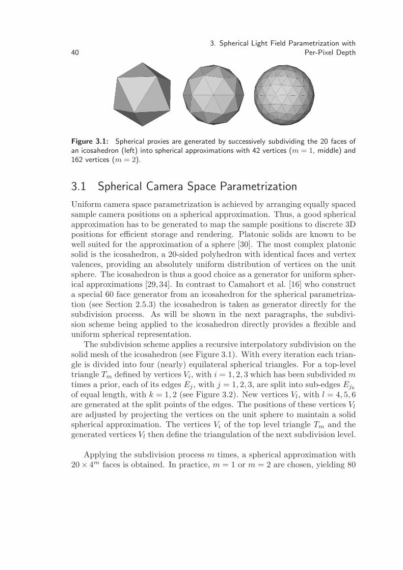
403. Spherical Light Field Parametrization with
Per-Pixel Depth
Figure 3.1: Spherical proxies are generated by successively subdividing the 20 faces ofan icosahedron (left) into spherical approximations with 42 vertices (m = 1, middle) and162 vertices (m = 2).
3.1 Spherical Camera Space Parametrization
Uniform camera space parametrization is achieved by arranging equally spacedsample camera positions on a spherical approximation. Thus, a good sphericalapproximation has to be generated to map the sample positions to discrete 3Dpositions for efficient storage and rendering. Platonic solids are known to bewell suited for the approximation of a sphere [30]. The most complex platonicsolid is the icosahedron, a 20-sided polyhedron with identical faces and vertexvalences, providing an absolutely uniform distribution of vertices on the unitsphere. The icosahedron is thus a good choice as a generator for uniform spher-ical approximations [29,34]. In contrast to Camahort et al. [16] who constructa special 60 face generator from an icosahedron for the spherical parametriza-tion (see Section 2.5.3) the icosahedron is taken as generator directly for thesubdivision process. As will be shown in the next paragraphs, the subdivi-sion scheme being applied to the icosahedron directly provides a flexible anduniform spherical representation.
The subdivision scheme applies a recursive interpolatory subdivision on thesolid mesh of the icosahedron (see Figure 3.1). With every iteration each trian-gle is divided into four (nearly) equilateral spherical triangles. For a top-leveltriangle Tm defined by vertices Vi, with i = 1, 2, 3 which has been subdivided mtimes a prior, each of its edges Ej , with j = 1, 2, 3, are split into sub-edges Ejk
of equal length, with k = 1, 2 (see Figure 3.2). New vertices Vl, with l = 4, 5, 6are generated at the split points of the edges. The positions of these vertices Vl
are adjusted by projecting the vertices on the unit sphere to maintain a solidspherical approximation. The vertices Vi of the top level triangle Tm and thegenerated vertices Vl then define the triangulation of the next subdivision level.
Applying the subdivision process m times, a spherical approximation with20× 4m faces is obtained. In practice, m = 1 or m = 2 are chosen, yielding 80

3.1. Spherical Camera Space Parametrization 41
E1
E2
E3
V1
V2 V3
V1
V2 V3
V4
V5
V6
E11
E12
E21 E22
E31
E32
T0
V1
V2 V3
V6V4
V5
T0
Figure 3.2: The triangle subdivision scheme. A top-level triangle is subdivided intoequilateral subtriangles by applying an interpolatory subdivision scheme. The positions ofvertices resulting from subdiving an edge into equal sub-edges are adjusted by projectingthe vertices on the unit sphere to maintain a solid spherical approximation.
or 320 faces and 42 or 162 vertices, respectively. Note that finer triangulationsinclude all of the vertices of the top level triangulation. Thus, a coarsening ofa previously refined spherical approximation is easily achieved afterwards bydropping the inner vertices and adjusting the topology accordingly.
The quality and thus the uniformity of this spherical approximation canbe evaluated by means of the triangle fetch aspect ratio, i.e. the ratio of thelongest triangle edge and the shortest triangle edge within the spherical ap-proximation. The ideal spherical approximation defines discrete vertices tobe positioned on the surface of the sphere such that a perfect equilateral tri-angulation can be established which yields an overall optimal triangle aspectratio of 1.0. As the subdivision process presented above is initiated based onan icosahedron yielding an equilateral triangulation based on 12 discrete posi-tions, this representation provides good spherical approximations. An averagefetch aspect ratio of 1.12 is achieved using the proposed subdivision process(see Table 3.1). Compared to spherical parameterizations being presented in
Sphere Maximum Minimum AverageResolution Sample Distance Sample Distance Sample Distance
12 1.051462 1.051462 1.05146242 0.618034 0.546533 0.582284
162 0.324920 0.275904 0.299332642 0.164647 0.138283 0.15073
Table 3.1: Sample distances of spherical parameterizations at different subdivision levels

423. Spherical Light Field Parametrization with
Per-Pixel Depth
the past (see Section 2.5.3) only a fractional part of discrete spherical samplepositions is being used in this spherical representation.
The spherical approximation is stored explicitly as an indexed face set, witheach of the vertices defining a sample position. For each vertex, a 4×4 viewingmatrix is stored which represents the transformation of world to sample cameracoordinates. This matrix is interpreted as extrinsic sample camera parameterfor light field acquisition as well as for reconstruction purposes. This sphericalapproximation of camera positions is denoted as camera sphere in the following.
3.2 Parabolic Image Space Parametrization
To capture the spherical light field according to the spherical camera spaceparametrization, the radiance along rays has to be captured at each of thediscrete sample positions defined by the camera sphere (see Section 3.1). Theuse of environment maps to capture the incoming light in a texture map hasbeen proven to be an efficient way for representing the radiance along rayspassing through a certain point in space [11]. As environment maps record theincident light passing through a single point in space from different directions,each individual environment map of a scene describes a concrete sample ofthe plenoptic function [73]. In the presented image space parametrization, araster image of the opposing hemisphere is stored using environment mappingtechniques for each camera of the camera sphere.
3.2.1 Environment Mapping Techniques
Various environment mapping techniques have been published in the past. Theapproaches, however, differ in sampling quality and applicability in the contextof light field sampling.
Cubic Environment Maps Cubic environment maps [37, 126] utilize sixindependent perspective images to capture the environment for a predefinedposition in 3D space. Each of these six images is captured from the center ofa cubical setup through each of its faces [36]. Cube maps are either storedusing six independent textures or in a single texture using texture atlas tech-niques [81] to merge these images into a single image based representation.This cubic representation shows fairly good sampling rates. 2D sampling ratesdiffer by a factor of 3
√3 (≈ 5.2) over all directions. This can be easily shown
through the following considerations. If a cube map sample has a differentialarea dA which corresponds to the pixel area of a single pixel within the cubicalmap, the solid angle covered by this pixel is thus the projection of dA onto

3.2. Parabolic Image Space Parametrization 43
the unit sphere. With n being a unit vector from the origin, dA being thedifferential areas of a pixel, and r being the distance from the origin to thepixel, the solid angle of a pixel (dω) is given by:
dω =ndA
r2(3.1)
To compute the solid angle explicitly, equation 3.1 is rewritten in cartesiancoordinates using
ndA = cosφ dx dy
r2 = x2 + y2 + z2
and
cosφ =z
r
=z√
x2 + y2 + z2
Considering the planar patch which is located at z = 1 and has its sides parallelto the x and y axes, the solid angle is calculated as follows.
dω =z dx dy√
x2 + y2 + z2· 1x2 + y2 + z2
=z dx dy
(x2 + y2 + z2)32
Thus, for the central pixel of a single patch of the cubic map, with x = 0, y = 0,and z = 1 the solid angle is dω = 1sr. For the corner pixel with x =+
− 1, y =+− 1,
and z = 1 however, the solid angle is dω = 13√
3sr. Pixels in the corner regions
of the cubical environment map cover only 13√
3of the solid angle covered by
center pixels. This means that these corner regions are sampled at a higherrate than the central directions [40].
Spherical Environment Maps A wide spread environment mapparametrization used in the computer graphics community is called spheri-cal environment mapping [38, 75]. Spherical environment maps are based onthe analogy of a small, perfectly mirroring metal ball centered around an ob-ject of interest. A single image that an orthographic camera captures whenfocusing on such a ball from a certain viewing direction can be interpreted asthe spherical environment map. Thus, spherical environment maps are moreefficient with respect to memory consumption compared to cube maps, as only

443. Spherical Light Field Parametrization with
Per-Pixel Depth
Figure 3.3: Left:The rays of an orthographic camera reflected off a paraboloid sample acomplete hemisphere of directions. Middle and Right: Sample textures of a parabolicallymapped synthetic environment. Images courtesy of Heidrich [41].
one single image is needed to represent the environment. However, this spher-ical parametrization exhibits areas of poor sampling [40]. Spherical environ-ment maps show maximum sampling rates for directions opposing the viewingdirection and reach sampling rates close to zero for directions similar to theviewing direction. Additionally, a singularity is observed with the sphericalparametrization. All points on the sphere with a viewing vector tangential tothe sphere show the same point of the environment.
Parabolic Environment Maps Parabolic environment mapping utilizestwo environment textures to perform a parabolic environment mapping [41].The idea behind the parabolic environment mapping technique is similar to thatof spherical mapping. Instead of generating the texture by recording the reflec-tion of the environment off a sphere, however, two paraboloids are used, eachof which covering an environment hemisphere [2]. For the proposed geometryit can be shown that the reflected rays in each point of the the paraboloid alloriginate from the a single point, the focal point of the paraboloid (see dashedlines in Figure 3.3). Thus, the complete environment can be stored in twoseparate circular textures, each containing the information of one hemisphere.Then, the reflection vectors are mapped to parabolic texture coordinates (u, v)according to Equation 3.2.1, 3.2.1. Note, that the sign of the z-componentof the reflection vector is used to decide which of the two textures is to beaccessed.
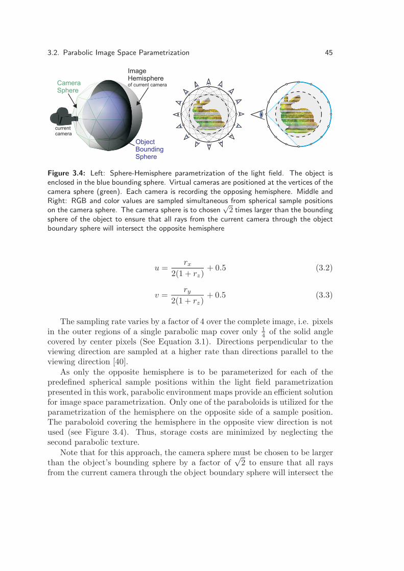
3.2. Parabolic Image Space Parametrization 45
ImageHemisphereof current camera
ObjectBoundingSphere
currentcamera
CameraSphere
Figure 3.4: Left: Sphere-Hemisphere parametrization of the light field. The object isenclosed in the blue bounding sphere. Virtual cameras are positioned at the vertices of thecamera sphere (green). Each camera is recording the opposing hemisphere. Middle andRight: RGB and color values are sampled simultaneous from spherical sample positionson the camera sphere. The camera sphere is to chosen
√2 times larger than the bounding
sphere of the object to ensure that all rays from the current camera through the objectboundary sphere will intersect the opposite hemisphere
u =rx
2(1 + rz)+ 0.5 (3.2)
v =ry
2(1 + rz)+ 0.5 (3.3)
The sampling rate varies by a factor of 4 over the complete image, i.e. pixelsin the outer regions of a single parabolic map cover only 1
4 of the solid anglecovered by center pixels (See Equation 3.1). Directions perpendicular to theviewing direction are sampled at a higher rate than directions parallel to theviewing direction [40].
As only the opposite hemisphere is to be parameterized for each of thepredefined spherical sample positions within the light field parametrizationpresented in this work, parabolic environment maps provide an efficient solutionfor image space parametrization. Only one of the paraboloids is utilized for theparametrization of the hemisphere on the opposite side of a sample position.The paraboloid covering the hemisphere in the opposite view direction is notused (see Figure 3.4). Thus, storage costs are minimized by neglecting thesecond parabolic texture.
Note that for this approach, the camera sphere must be chosen to be largerthan the object’s bounding sphere by a factor of
√2 to ensure that all rays
from the current camera through the object boundary sphere will intersect the

463. Spherical Light Field Parametrization with
Per-Pixel Depth
Figure 3.5: Five image samples taken for a spherical light field with 42 cameras. Eachimage represents a parabolic mapping of the hemisphere for color (top row) and depth(bottom row).
opposite hemisphere (see Figure 3.4). For each of the spherical camera positionsthe opposite hemisphere is then mapped to a parabolic representation. For eachray emerging from a sample camera position and intersecting the camera sphereat the opposite hemisphere at point S the radiance is mapped to parabolictexture coordinates (u, v) as follows:
(uv
)k
=12
⎛⎝ sx
1 + sz+ 1
sy
1 + sz+ 1
⎞⎠
k
with Sk =
⎛⎝ sx
sy
sz
⎞⎠
k
(3.4)
In practice, a resolution of 256 × 256 or 512 × 512 pixels is chosen for theparabolic texture. Examples of source images for the light field are displayedin Figure 3.5.
3.3 Geometric Representation
The light field samples acquired from the spherical arrangement of samplepositions is supplemented by a representation of the captured scene’s geometry.For efficiency reasons a depth map is stored with every light field sample beingacquired. Depth maps store the geometry distance for individual rays on aper-pixel basis. The depth map is generated with a resolution according to thelight field sample resolution. Using the alpha channel of a captured paraboliclight field sample, the depth can efficiently be stored in the fourth channel of

3.4. Sampling Analysis 47
zmaxz'
Figure 3.6: The depth value is obtained by dividing the bounding-object distance z′ bythe bounding sphere’s secant length zmax.
the RGBA parabolic map (see Figure 3.5). In the remainder of this work RGBtextures with a depth value stored in the alpha channel are referred to as RGBztextures.
Per-pixel depth values are calculated for each ray as the distance z′ fromthe first intersection point with the object’s bounding sphere to the objectsurface. The ratio of z′ to the bounding sphere’s ray secant length zmax isthen stored as the final depth in the alpha channel of the parabolic textureaccording to Figure 3.6. This results in a depth value between 0 and 1, whichcan efficiently be stored as 8 bit value in the alpha channel [86]. Applying an 8bit quantization on the geometric domain with a depth complexity of 1 yields256 depth layers, each of which covering a depth interval of 1/256(≈ 0.004).
3.4 Sampling Analysis
According to the Nyquist theorem, in order for a signal to be reconstructedwithout aliasing the sampling frequency needs to be greater then the Nyquistrate. Chai et al. [17] determine the maximum distance for adjacent samplecamera positions (Δscmax) from the maximum sample rate in the image domain(Δsi), according to:
Δscmax =1
2Δsi(3.5)
Thus, while limiting the acquisition of light field samples to a uniform imagespace sampling resolutions in both directions (Δsi) of 256, 512 and 1024, amaximum geometric distance of ≈ 0.002, ≈ 0.0009 and ≈ 0.0005, respectivelyfor adjacent sample positions is not to be exceeded in order for the light field

483. Spherical Light Field Parametrization with
Per-Pixel Depth
synthesis to be performed without aliasing artifacts (see Equation 3.2).While Chai et al. defined the maximum distance for adjacent sample posi-
tions from a spectral analysis of a 4D light field parameterized using the twoplane approach, it can be shown that this analysis also holds for the sphericalparametrization presented in this work. Considering the polygonal approxi-mation of the sphere which defines the sample positions in this spherical lightfield approach, a set of three adjacent sample positions do lie in a commonplane. Under this assumption the spherical approximation can be regarded tobe locally planar. The, the sampling analysis of Chai et al. also hold for alocal observation of sampling space of the spherical parametrization presentedin this work.
Chai et al. further show, that for a given image space sampling rate, themaximum sampling distance can be increased, if geometric depth informationis available with each light field sample being acquired. For Nd discrete levelsof depth quantization being available, the maximum sampling camera distanceis then determined by:
Δscmax
Nd=
12Δsi
(3.6)
Δscmax =Nd
2Δsi(3.7)
For an 8 bit depth quantization yielding 256 discrete levels of depth, themaximum sampling camera distance (scmax) can then be extended to 0.5, 0.25and 0.125 for image space sampling (Δsi) of 256, 512 and 1024, respectively.Thus, with an 8 bit depth representation being available, camera sphere rep-resentations resulting from subdividing the initial icosahedron m ≥ 2 timesrepresent good sampling schemes.
For a subdivision level of m ≥ 2, the spherical sample setup satisfies themaximum sampling distance constraint (see Table 3.1). Depending on theimage space resolution subdivision levels of increased sampling density may bechosen to avoid aliasing artifacts.
3.5 Storage Efficiency and Light Field Compression
The storage efficiency of the light field representation presented above is de-pendent on the resolution of both, the resolution of the sample image and thesample position density. For each sample position an individual 2D RGBz tex-ture map is stored. Storage costs per sample image (Mems) are steered by the

3.5. Storage Efficiency and Light Field Compression 49
image sampling rate si as follows:
Mems = si × si × 4 byte (3.8)
In practice, light field samples are captured at a resolution of 256 × 256 and512 × 512 yielding per sample storage costs of 256Kbyte and 1024Kbyte.
The storage costs caused by each light field sample texture are multipliedby the amount of camera sample positions (Nc) for the complete light fieldrepresentation. Additional storage costs are caused by storing the sphericalapproximation being stored explicitly as an indexed face set. Remember, witheach vertex, a 4×4 viewing matrix is stored which represents the sample cameracoordinate transformation. Storing the viewing matrices using 4 byte floatingpoint values and an index list containing 20× 4m ∗ 3 short integer values (withm being the spherical subdivision level) the total memory consumption for acomplete light field representation (Memlf ) is then computed according to:
Memlf = Nc × Mems + Nc × 16 × 4 + 20 × 4m × 3 × 2 bytes (3.9)
Typical sizes of light field representations for a variety of image- and cameraspace resolutions are listed in Table 3.2.
Images Resolution Uncompressed S3TC DXT3 S3TC DXT3 & zipped12 256 × 256 3.1 MB 0.7 MB 0.2 MB12 512 × 512 12.3 MB 3.0 MB 0.5 MB42 256 × 256 10.8 MB 2.7 MB 0.6 MB42 512 × 512 43.0 MB 10.8 MB 1.5 MB
162 256 × 256 41.5 MB 10.4 MB 1.9 MB162 512 × 512 165.9 MB 41.5 MB 5.9 MB642 256 × 256 164.4 MB 41.1 MB 7.5 MB642 512 × 512 657.5 MB 164.4 MB 23.5 MB
Table 3.2: Sizes of typical light fields with and without compression
To reduce the amount of graphics memory consumed by the parabolicmaps, commodity hardware-accelerated texture compression schemes can beemployed. S3TC texture compression [48] offers an effective and easy way tocompress the light field images. Five different variants of the S3TC compres-sion algorithm are available (named DXT1 through DXT5) which all store a4 × 4 block of pixels in a 64-bit or 128-bit quantity and achieve a compressionratio of 8:1 or 4:1. The DXT5 algorithm works on RGBA textures, stores a128-bit value per 4 × 4 pixel block, and achieves a compression ratio of 4:1.

503. Spherical Light Field Parametrization with
Per-Pixel Depth
In our storage scheme, however, the alpha portion contains the depth values,which turned out to be sensitive to compression artifacts resulting from a blockwise compression. This is especially critical at object boundaries. Fecker etal. [28] demonstrated that a block wise compression of a scenery’s depth infor-mation will cause noticeable loss of quality within light field synthesis. Thus,the DXT3 compression algorithm is used to maintain best results within therendering task. DXT3 works on RGBA data as well, but does store an explicitalpha value per pixel. DXT3 also stores a 128-bit value per 4 × 4 pixel block,but an additional 4-bit alpha value per pixel. Alpha values are compressed ona per pixel basis. Thus, artifacts resulting from a block wise compression to donot occur. DXT3 still offers a total compression ratio of 4:1. DXT1, DXT2,and DXT4 compression schemes do only provide very primitive alpha channelsupport. For this reason, these compression schemes are not applicable to theRGBz data representation being used in this work.
A light field being generated using the proposed spherical parametrizationwith 162 images and a resolution of 512× 512 pixels consumes 165.9 MB with-out compression. In comparison, a DXT3 compressed light field of the samedimensions consumes only 41.5 MB of memory. For storing and transmission,the total size of a light field data set can be further reduced significantly byapplying standard ZIP compression techniques. With both ZIP and DXT3texture compression the same light field is reduced to a average size of about6 MB (See Table 3.2).
3.6 Conclusion
The spherical light field parametrization with per-pixel depth presented in thischapter represents an innovative parametrization approach which implementsa uniform sampling of both position and direction. For the directional domain,however, a parabolic image based representation is applied which does providea good approximation of a uniform sampling pattern for the directional domain.Here, the parabolic representation was chosen due to its storage efficiency. Theproposed parametrization opens up for virtual view synthesis with 6 DOF forvirtual viewpoint selection. It implements an efficient light field representationwith respect to storage costs which includes an implicit geometric scene de-scription at minimum additional storage costs based on per-pixel depth values.Light field samples and depth values are stored in a common RGBz parabolictexture map which opens up for standard texture compression techniques tofurther reduce storage costs.
In contrast to the two plane light field rendering approach presented

3.6. Conclusion 51
TwoPlane
DataRepresentation
GeometryRepresentation
Sampling Uniformity
UniformOrientation
NonUniform
UniformPosition
DirectRendering
Processingon Rendering
Pre-processing
UniformPosition &Orientation
NoGeometry
ExplicitGeometry
ImplicitGeometry
Lumigraph
Spherical
TwoSphere
SpherePlane
UnstructuredLumigraph
FreeformLight Field
SphereHemisphere
Figure 3.7: Categorization of the sphere-hemisphere fight field parametrization presentedin this chapter.
by Levoy and Hanrahan [63] (see Section 2.5.1) this spherical light fieldparametrization implements a sampling scheme which allows the virtual view-point and virtual view direction to be chosen freely with 6 DOF for virtual viewsynthesis. The parametrization is chosen sparse enough to open up for efficientstorage schemes, but dense enough to allow arbitrary views to be reconstructedwithout noticeable artifacts. Discontinuities as observed with the lumigraphapproach presented by Gortler et al. [35] (see Section 2.5.2) are avoided due tothe spherical parametrization being invariant under both translation and ro-tation. Contrary to free form lightfields [97] and unstructured lumigraphs [13](see Section 2.5.4) a uniform representation is guaranteed with this sphericalparametrization.
The uniform spherical parametrization presented in this chapter is akin tothe representations applied for spherical light field rendering presented by Ihmet al. [47] and Camahort et al. [16] (see Section 2.5.3). However, essential lesslight field sample positions (-90–95%) are needed to sample a complete lightfield. Storing an 8 bit depth value with every captured ray in a common RGBz

523. Spherical Light Field Parametrization with
Per-Pixel Depth
parabolic texture map, provides 256 distinct depth layers that significantlyreduce the amount of necessary light field samples (see Section 3.4).
With the depth being stored per pixel within the same texture based repre-sentation it is accessible directly in conjunction with the RGB data from withina single texture fetch. As will be shown in the following chapter, the proposedrepresentation provides an efficient light field parametrization which facilitateslight field synthesis without the need for expensive geometry processing andtopology adjustments. The light field representation satisfies the need for auniform sampling which implements an implicit geometry representation of thescene and provides direct view synthesis capabilities. A comparison to lightfield parameterizations presented in the past is illustrated in Figure 3.7.
The parametrization presented in this chapter has been presented to thecomputer graphics community by Todt et al. [117, 120].

4
Spherical Light FieldRendering with Per-Pixel
Depth
In this chapter a light field rendering approach is presented which is based onthe sphere-hemisphere light field parametrization with per-pixel depth beingintroduced in chapter 3. The rendering technique exploits the uniform sam-pling structure and implicit geometric representation to implement an efficientlight field synthesis from a sparsely sampled light field representation. Depthcorrection of rays based on the proposed depth map representation allows forhigh-quality virtual view generation at real-time frame rates without ghost-ing or disparity artifacts. Virtual viewpoints can be chosen with 6 DOF forpositions outside the convex hull of the represented object.Image synthesis is implemented on the graphics processing unit (GPU) as afragment program which efficiently extracts correct image information fromadjacent cameras for each fragment by applying per-pixel depth correction ofrays based on the parabolic texture representation of image space. Texturesamples are exploited within the view synthesis directly without the need forfurther complex and costly geometry processing or structural topology adjust-ments.
Two different rendering implementations are introduced in this chapter.While one rendering algorithm implements an iterative refinement approachfor rendering light fields, the other approach implements a raycasting techniquewhich provides superior rendering quality at moderate frame rates.
The rendering techniques are parameterized to be adjustable by means ofperformance and quality to adapt to changing requirements. Level of detailrendering techniques have been implemented to account for varying object dis-tance and visibility. The optimized rendering techniques allow multiple lightfields to be rendered synchronously to generate complex scenes. The efficiencyof the uniform light field parametrization in combination with the renderingtechnique’s flexibility provides a solid fundament for the implementation of a
53

54 4. Spherical Light Field Rendering with Per-Pixel Depth
web-based remote light field renderer based on a client-server architecture toprovide remote access to light field representations of complex scenes.
This chapter describes the GPU based spherical light field rendering withper-pixel depth in detail. The iterative refinement rendering approach and theraycasting technique are explained in the first three sections, followed by a de-scription of level of detail rendering for light fields in the fourth section. Thefifth section comprehensively describes progressive light field rendering imple-mented for remote access to light field data based on a client-server architecture.This chapter is closed with a conclusion in the sixth section.
4.1 Spherical Light Field Rendering
For both of the two light field rendering approaches presented in this chapter,the light field is rendered by rasterizing the front faces of the polygonal camerasphere representation with respect to the virtual viewpoint (Peye). The virtualviewpoint can be chosen with 6 DOF to lie anywhere outside the sphericalcamera space representation. However, the viewpoint is restricted to be locatedoutside the camera sphere to avoid the vertices of the front faces being culledby frustum culling. Remember, each vertex of the camera sphere correspondsto a pre-defined camera sample position (C) (see Section 3.1).
The polygonal mesh is rendered by drawing the set of triangles from apredefined OpenGL display list [78] according to the concrete spherical repre-sentation of the light field. For each triangle each of its vertices is assignedone of three distinct color values, namely red (glColor3f(1.0f,.0f,.0f))for camera C0, green (glColor3f(.0f,1.0f,.0f)) for camera C1, and blue(glColor3f(.0f,.0f,1.0f)) for camera C2. These vertex colors are inter-preted as interpolation weights within the light field synthesis. Additionallythe parabolic RGBz texture image, the transformation matrix M of the camera,and the background color are bound as parameters to each of the vertices.
While a common vertex program is utilized which implements standard ver-tex operations, a customized fragment program is implemented which performsthe light field synthesis based on the input parameters (see Figure 4.1). Theinput parameters such as the sample camera transformation and per-vertexinterpolation weights are passed through to the fragment program by the ver-tex shader. The vertex positions, however, are transformed according to themodelview-projection matrix of the current virtual view.
Within rasterization, per-vertex camera blending weights are interpolatedfor each triangle being rendered. Within the fragment program interpolatedcolor values and thus interpolated camera weights are available per fragment.

4.1. Spherical Light Field Rendering 55
Polygonal SphereSetupInitiate triangle meshwith per-pixel vertexinterpolation weightsas colors
Per-FragmentLight FieldSynthesisDetermine final fragmentcolor
Displaysynthesized view
ViewingTransformationProcess vertices andpass colors, textures &camera interpolationweights
Figure 4.1: Overview of the light field synthesis process. The polygonal mesh of thespherical representation is rendered to synthesize virtual views. A common vertex programimplements standard vertex operations and passes per-vertex shader parameters to thefragment program. The customized fragment program performs the light field synthesisto generate a virtual view.
The final color is then determined within the customized fragment programbased on the light field synthesis technique. Both of the light field synthesistechniques presented in the following sections implement a specific fragmentshader which samples the input textures to extract light field sample data andper-pixel depth values in order to synthesize high quality virtual views.
Note, however, that in practice the RGB and depth information of theparabolic map are bound as separate texture objects. While the RGB texturecan be linearly interpolated using OpenGL’s standard GL LINEAR interpolationscheme, noticeable render artifacts at the silhouettes appear when interpolatingthe depth information. Using the nearest neighbour texture lookup scheme(GL NEAREST) ensures appropriate depth information per pixel and avoids depthaliasing artifacts at object boundaries.
V0
V1 V2
T0
T1 T2
Figure 4.2: Rendering of the polygonal camera sphere representation with distinctcolors being assigned to each of a triangle’s three vertices. For each vertex a color valuerepresenting the sample camera blending weight, the input RGBz texture Tn, and thecorresponding camera’s transformation matrix are assigned.

56 4. Spherical Light Field Rendering with Per-Pixel Depth
InitializationInitialize parametersand variables
Initial SamplingGet initial depth valuesfor inital intersection
IterativeRefinementEstablish ray - objectintersection candidates
FinalInterpolationInterpolate colors andcalculate fragment’sdepth
All surfacepoints inEpsilon?
no yes
Max.iterationsreached?
no
yes
Figure 4.3: The iterative refinement approach employs four sequential steps to establishcoherent rays and thus coherent light field samples per fragment.
4.2 Iterative Refinement
The iterative refinement technique is outlined in Figure 4.3. Four sequentialsteps are implemented within this light field synthesis approach to establishcoherent rays and thus coherent light field samples in order to determine thefinal fragment color (see Figure 4.4).
First, all variables and parameters, such as the current viewing positionand viewing direction are initialized in the initialization step. For the currentfragment, a viewing ray is established based on the viewing direction. Thisray’s intersection with the opposite hemisphere of the spherical representationis evaluated to determine initial texture coordinates and thus initial texturefetches. Based on the initial depth values being extracted from the texturefetch’s alpha channel a first object intersection is assessed. The first intersec-tion estimate is then successively refined in the subsequent iterative refinementstep. With a ray-object intersection being reliably determined in the itera-tive refinement process, the final fragment color is evaluated by interpolatingappropriate texture fetches.
4.2.1 Iterative Refinement Process
When a triangle is rasterized, each fragment corresponds to a unique positionV on the camera sphere. In the first step, the fragment program calculates theintersection point of the viewing ray with the camera sphere to obtain a firstestimate of the object intersection point P
(0)obj. The superscript in this notation
refers to the iteration count (see Figure 4.4).

4.2. Iterative Refinement 57
Second iteration
Peye
Pobj(0)
Pcam,0(0)
Pcam,1(0)
First Iteration
C0
C1
(0)=Pcam,k
^C0
C1(1)
Pcam,1^
(1)Pcam,0^
Pcam,0(1)
Pcam,1(1) Pobj
(1)V
Figure 4.4: First and second step of the iterative depth refinement.
The calculated intersection point is transformed into the viewing space ofcamera k according to
S(i)k = Mk P
(i)obj with k ∈ {0, 1, 2}. (4.1)
This is done for each of the three adjacent cameras that correspond tothe original triangle’s vertices. The sphere intersection points Sk can now beconverted to parabolic texture coordinates (u, v) , according to
(uv
)k
=12
⎛⎝ sx
1+ sz+ 1
sy
1+ sz+ 1
⎞⎠
k
with Sk =
⎛⎝ sx
sy
sz
⎞⎠
k
. (4.2)
RGBz samples are obtained from the parabolic texture maps corresponding tothe three cameras. The depth value z is extracted from the alpha portion and isused to calculate the camera’s local estimate P
(i)cam,k for the object intersection
point:
P(i)cam,k = z · Ck + (1 − z) P
(i)cam,k (4.3)
with P(i)cam,k being the object intersection point and P
(i)cam,k the intersection
point being projected onto the sphere using Ck as center of projection. Notethat Equation 4.3 is a simple linear interpolation, because z stores the depthvalue as fractional part of the secant length.
An improved estimate for the object intersection point Pobj can now befound by projecting the three local camera distances onto the viewing ray andcalculating the average, according to:
P(i+1)obj = V +
13
2∑k=0
((P (i)cam,k − Ck) · r) r (4.4)

58 4. Spherical Light Field Rendering with Per-Pixel Depth
with r being the normalized direction of the original viewing ray (red line).As illustrated in Figure 4.4, the iteration can be pursued several times by
projecting the updated object point P(i+1)obj onto the sphere using the cam-
era vertices Ck as center of projection. The resulting intersection points aresuccessively transformed into camera coordinates to establish depth values, todetermine improved local estimates according to Equation 4.3, and eventuallycalculate an improved intersection point according to Equation 4.4.
The procedure is terminated if the desired accuracy is achieved or a max-imum number of iterations is reached. The maximum number of iteration isadjustable at runtime. In practice, however, a maximum number of iterationsof 5 turned out to be sufficient.
Accuracy is steered by an adjustable error threshold. The error thresholdparameter defines the maximum distance of local estimates (P (i)
obj) determinedwithin the iterative refinement process. In case of the maximum divergenceof local estimates falling below the error threshold the iteration procedure isterminated. Obviously, ray coherence and as a consequence image synthesisquality is maximized with the error threshold parameter being minimized.
The final color of the fragment is calculated as the weighted sum of the RGBvalues extracted from the parabolic textures of the different cameras withinthe final iteration. The weights for each camera correspond to the barycentriccoordinates of the fragment with respect to the original triangle. With theprimary colors red, green and blue being assigned to the three vertices dur-ing geometry setup, the correct weights are automatically calculated throughcolor interpolation during rasterization. With the latest local estimates beingaveraged and projected to viewing space according to the virtual viewpoint’smodelview-projection matrix a depth value is determined for each individualfinal fragment.
4.2.2 Implementation Details - Iterative Refinement
This section presents in depth details concerning implementation issues of thefour sequential steps being performed for light field synthesis within the frag-ment program (see Figure 4.3).
Initialization Within the initialization the fragment position is determinedfrom barycentric interpolation of the associated triangle’s vertex positions (cn)taking the input color as interpolation weights. The viewing direction (dir)and the normalized viewing direction (dirN) are established based on the vir-tual viewpoint position (Peye) and the current fragment’s position (v) (SeeAppendix A.1 ll. 31–33 for the corresponding code sequence).
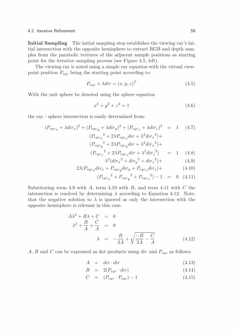
4.2. Iterative Refinement 59
Initial Sampling The initial sampling step establishes the viewing ray’s ini-tial intersection with the opposite hemisphere to extract RGB and depth sam-ples from the parabolic textures of the adjacent sample positions as startingpoint for the iterative sampling process (see Figure 4.5, left).
The viewing ray is noted using a simple ray equation with the virtual view-point position Peye being the starting point according to:
Peye + λdir = (x, y, z)T (4.5)
With the unit sphere be denoted using the sphere equation
x2 + y2 + z2 = 1 (4.6)
the ray - sphere intersection is easily determined from:
(Peyex + λdirx)2 + (Peyey + λdiry)2 + (Peyez + λdirz)2 = 1 (4.7)
(Peyex2 + 2λPeyexdir + λ2dirx
2)+
(Peyey2 + 2λPeyeydir + λ2dirx
2)+
(Peyez2 + 2λPeyezdir + λ2dirz
2) = 1 (4.8)
λ2(dirx2 + diry
2 + dirz2)+ (4.9)
2λ(Peyexdirx + Peyeydiry + Peyezdirz)+ (4.10)
(Peyex2 + Peyey
2 + Peyez2) − 1 = 0 (4.11)
Substituting term 4.9 with A, term 4.10 with B, and term 4.11 with C theintersection is resolved by determining λ according to Equation 4.12. Note,that the negative solution to λ is ignored as only the intersection with theopposite hemisphere is relevant in this case.
Aλ2 + Bλ + C = 0
λ2 +B
A+
C
A= 0
λ = − B
2A+
√−B
2A− C
A(4.12)
A, B and C can be expressed as dot products using dir and Peye as follows:
A = dir · dir (4.13)B = 2(Peye · dir) (4.14)C = (Peye · Peye) − 1 (4.15)

60 4. Spherical Light Field Rendering with Per-Pixel Depth
44 //determine viewing ray - sphere intersection on opposite hemisphere45 float A,B,C;46 C = dot(P eye,P eye) - 1.0;47 B = 2.0 * dot(P eye,dir);48 A = dot(dir,dir);4950 float S = max( (B*B - 4.0 * A*C) ,0.0); //components under sqrt51 //ignore negative solution - opposite hemisphere, only52 float lambda = (-B + sqrt(S)) /A/2.0;5354 //Sphere intersection55 float3 vecS = (P eye + lambda * dir);
Code Sample 4.1: Initial intersection of the viewing ray with the opposite hemisphere,with respect to the current vertex.
Thus, with the use of the dot product the intersection of the viewing raywith the opposite hemisphere is efficiently calculated in the fragment program(see Code Sample 4.1).
From the initial intersection point, texture coordinates (u, v) are determinedaccording to Equation 4.2 for each adjacent sample camera to extract RGB anddepth values from the light field samples. With the depth information of theinitial sphere intersection to be known for each of the three sample cameras,the iterative sampling is initiated.
Iterative Sampling Within the iterative refinement phase, the initial inter-section point and the depth values being evaluated for each of the three ad-jacent sample cameras are used to determine a valid object intersection point(see Figure 4.5). First, local estimates are determined for each sample position.Then, a new sample position on the viewing ray is determined which is used inthe third step to determine error values for the three local estimates. For thenew viewing ray sample position the sphere intersection points are updated toestablish new depth values per sample camera. Based on the coherence of theupdated depth values the iteration is either terminated or restarted in case ofthe distance exceeding the given errorThreshold value.
1. Local Estimates: Local estimates are determined for each sample cameraby scaling the vector from the sample camera position to the last sphericalintersection point by the sampled depth according to Figure 4.5, left.
2. Update Viewing Ray Sample Position: The local estimates are projectedonto the viewing ray in order to determine the next sample position on theviewing ray. The updated sample position is determined from the average

4.2. Iterative Refinement 61
C1
C0
C1
C0
C1
C0
S
C1
C0
S
C1
C0
S
C1Sdepth C1S
C0S
depth C0S
DetermineLocal Estimates
Update SamplePosition
Project LocalEstimates ontoViewing Ray
All surfacepoints inEpsilon?
no yes
Final color interpolation
Figure 4.5: The iterative refinement phase in detail. Local estimates are determinedfor each adjacent sample camera by scaling the sampling ray C0S by the depth valuebeing sampled from the parabolic texture. These estimates are then projected onto theviewing ray in order to determine the new sampling position. If all of the local estimatesare positioned within a given error threshold, iteration is stopped.
position of the projected local estimates according to Equation 4.4 (seeFigure 4.5, middle and right). In case of more than half of the maximumiterations already processed, however, highly divergent object intersec-tions are assumed. In this case the interpolation operation is replaced bya maximum operation to avoid a deadlock situation (See Section 4.2.3).
3. Evaluate Error: For the interpolated new viewing ray sample position theabsolute distances to the three local estimates are chosen as error value toevaluate the validity of the reconstructed object intersection points. Theabsolute distances are weighted by the barycentric weights to ensure moredistant camera sample positions to have less influence on the overall error.The overall error is then determined as the squared sum of the absolutedistances.
4. Resample Parabolic Textures: For the updated viewing ray sample posi-tion, new spherical intersection points are established for each adjacentsample camera position according to the ray sphere intersection as per-formed in the initial step. The next iteration, however, is initialized only,if the evaluated error still exceeds the given errorThreshold.
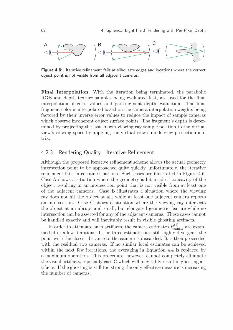
62 4. Spherical Light Field Rendering with Per-Pixel Depth
A B C
Figure 4.6: Iterative refinement fails at silhouette edges and locations where the correctobject point is not visible from all adjacent cameras.
Final Interpolation With the iteration being terminated, the parabolicRGB and depth texture samples being evaluated last, are used for the finalinterpolation of color values and per-fragment depth evaluation. The finalfragment color is interpolated based on the camera interpolation weights beingfactored by their inverse error values to reduce the impact of sample cameraswhich observe incoherent object surface points. The fragment’s depth is deter-mined by projecting the last known viewing ray sample position to the virtualview’s viewing space by applying the virtual view’s modelview-projection ma-trix.
4.2.3 Rendering Quality - Iterative Refinement
Although the proposed iterative refinement scheme allows the actual geometryintersection point to be approached quite quickly, unfortunately, the iterativerefinement fails in certain situations. Such cases are illustrated in Figure 4.6.Case A shows a situation where the geometry is hit inside a concavity of theobject, resulting in an intersection point that is not visible from at least oneof the adjacent cameras. Case B illustrates a situation where the viewingray does not hit the object at all, while at least one adjacent camera reportsan intersection. Case C shows a situation where the viewing ray intersectsthe object at an abrupt and small, but elongated geometric feature while nointersection can be asserted for any of the adjacent cameras. These cases cannotbe handled exactly and will inevitably result in visible ghosting artifacts.
In order to attenuate such artifacts, the camera estimates P(i)cam,k are exam-
ined after a few iterations. If the three estimates are still highly divergent, thepoint with the closest distance to the camera is discarded. It is then proceededwith the residual two cameras. If no similar local estimates can be achievedwithin the next few iterations, the averaging in Equation 4.4 is replaced bya maximum operation. This procedure, however, cannot completely eliminatethe visual artifacts, especially case C which will inevitably result in ghosting ar-tifacts. If the ghosting is still too strong the only effective measure is increasingthe number of cameras.
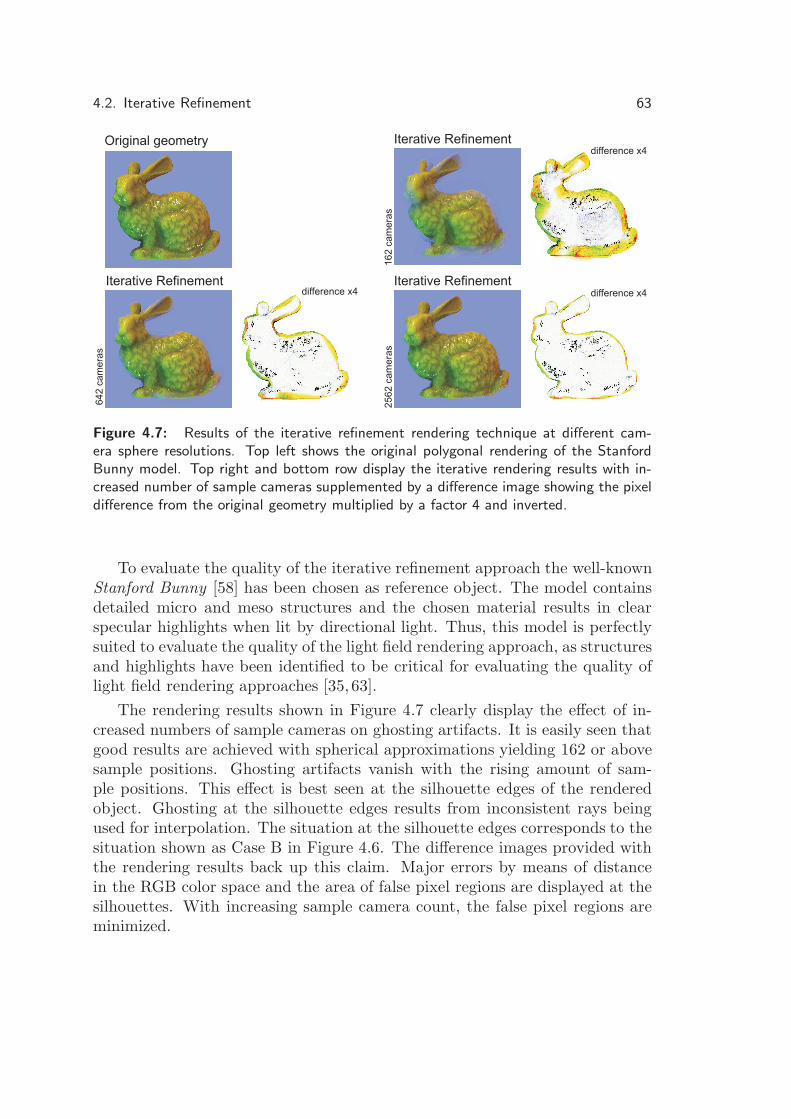
4.2. Iterative Refinement 63
Original geometry
16
2ca
me
ras
difference x4Iterative Refinement
25
62
ca
me
ras
difference x4Iterative Refinement
64
2ca
me
ras
difference x4Iterative Refinement
Figure 4.7: Results of the iterative refinement rendering technique at different cam-era sphere resolutions. Top left shows the original polygonal rendering of the StanfordBunny model. Top right and bottom row display the iterative rendering results with in-creased number of sample cameras supplemented by a difference image showing the pixeldifference from the original geometry multiplied by a factor 4 and inverted.
To evaluate the quality of the iterative refinement approach the well-knownStanford Bunny [58] has been chosen as reference object. The model containsdetailed micro and meso structures and the chosen material results in clearspecular highlights when lit by directional light. Thus, this model is perfectlysuited to evaluate the quality of the light field rendering approach, as structuresand highlights have been identified to be critical for evaluating the quality oflight field rendering approaches [35, 63].
The rendering results shown in Figure 4.7 clearly display the effect of in-creased numbers of sample cameras on ghosting artifacts. It is easily seen thatgood results are achieved with spherical approximations yielding 162 or abovesample positions. Ghosting artifacts vanish with the rising amount of sam-ple positions. This effect is best seen at the silhouette edges of the renderedobject. Ghosting at the silhouette edges results from inconsistent rays beingused for interpolation. The situation at the silhouette edges corresponds to thesituation shown as Case B in Figure 4.6. The difference images provided withthe rendering results back up this claim. Major errors by means of distancein the RGB color space and the area of false pixel regions are displayed at thesilhouettes. With increasing sample camera count, the false pixel regions areminimized.

64 4. Spherical Light Field Rendering with Per-Pixel Depth
Images MAE MSE RMSE PAE162 0,0413227 0,0151801 0,123207 0,968627642 0,0253391 0,0082435 0,090794 0,954314
2562 0,0145189 0,0042915 0,065510 0,949020
Table 4.1: Per-pixel color differences of the synthesized image compared to the originalrendering. Mean absolute error, mean squared error, and root mean squared error aredisplayed for light field renderings being synthesized from a varying amount of inputsamples.
The visual appearance of concavities and small-to-large depth variationsare reconstructed at good quality. The structured surface of the original 3Drendering is clearly resampled in the light field rendering. Concavities as theyoccur in the transition zone between the bunny’s body and his hind legs arereconstructed precisely. The difference image does not show significant pixeldifferences in these regions. Local differences, however, are observed at thespecular highlights which occur in regions of great curvature all over the object’ssurface. Even with an increased amount of sample cameras this highlight errorcannot be reduced significantly.
The observation is approved by a statistical analysis of per-pixel RGB dif-ferences. Table 4.1 shows the mean absolute error (MAE), the mean squarederror (MSE), the root mean squared error (RMSE), and the peak absolute er-ror of any one pixel within an RGB channel (PAE) for the spherical light fieldrepresentation being displayed in Figure 4.7. From the table it can be seenclearly that all of the error measures significantly drop with rising amount ofsample positions. While the RMSE is reduced by about 25% with an increaseof sample positions from 162 to 642, the RMSE is halved by using 2562 samplepositions instead of 162 samples. The PAE, however, remains constantly highthroughout all configurations of sample positions. While the absolute peakerror reflects the maximum distance of any one pixel within an RGB channel,it can be easily seen that a single pixel which does not correspond to the sameRGB value in the original image will result in a high PAE. From the differenceimages shown in Figure 4.7 it can be seen that significant per-pixel differencesoccur at the highlights of the object. As a consequence these false pixels resultin the high PAE.
While the sample camera arrangement is chosen to be dense for the iter-ative rendering approach, far less samples are required compared to sphericalrendering approaches presented in the past (see Section 2.5.3) to achieve com-parable rendering quality. Thus, light fields can be reconstructed from more
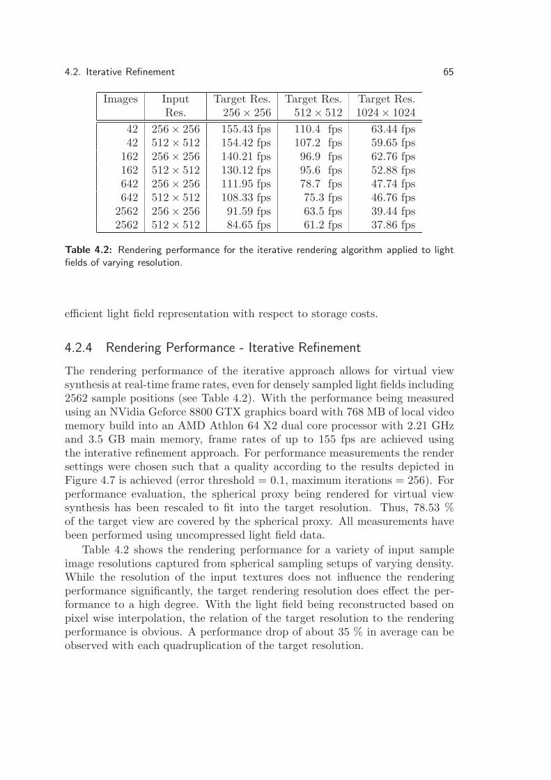
4.2. Iterative Refinement 65
Images Input Target Res. Target Res. Target Res.Res. 256 × 256 512 × 512 1024× 1024
42 256 × 256 155.43 fps 110.4 fps 63.44 fps42 512 × 512 154.42 fps 107.2 fps 59.65 fps
162 256 × 256 140.21 fps 96.9 fps 62.76 fps162 512 × 512 130.12 fps 95.6 fps 52.88 fps642 256 × 256 111.95 fps 78.7 fps 47.74 fps642 512 × 512 108.33 fps 75.3 fps 46.76 fps
2562 256 × 256 91.59 fps 63.5 fps 39.44 fps2562 512 × 512 84.65 fps 61.2 fps 37.86 fps
Table 4.2: Rendering performance for the iterative rendering algorithm applied to lightfields of varying resolution.
efficient light field representation with respect to storage costs.
4.2.4 Rendering Performance - Iterative Refinement
The rendering performance of the iterative approach allows for virtual viewsynthesis at real-time frame rates, even for densely sampled light fields including2562 sample positions (see Table 4.2). With the performance being measuredusing an NVidia Geforce 8800 GTX graphics board with 768 MB of local videomemory build into an AMD Athlon 64 X2 dual core processor with 2.21 GHzand 3.5 GB main memory, frame rates of up to 155 fps are achieved usingthe interative refinement approach. For performance measurements the rendersettings were chosen such that a quality according to the results depicted inFigure 4.7 is achieved (error threshold = 0.1, maximum iterations = 256). Forperformance evaluation, the spherical proxy being rendered for virtual viewsynthesis has been rescaled to fit into the target resolution. Thus, 78.53 %of the target view are covered by the spherical proxy. All measurements havebeen performed using uncompressed light field data.
Table 4.2 shows the rendering performance for a variety of input sampleimage resolutions captured from spherical sampling setups of varying density.While the resolution of the input textures does not influence the renderingperformance significantly, the target rendering resolution does effect the per-formance to a high degree. With the light field being reconstructed based onpixel wise interpolation, the relation of the target resolution to the renderingperformance is obvious. A performance drop of about 35 % in average can beobserved with each quadruplication of the target resolution.

66 4. Spherical Light Field Rendering with Per-Pixel Depth
InitializationInitialize parametersand variables
Initial Sample PosDetermine first sampleposition on viewing ray
RaycastingSample ray at equi-distant sample positions
FinalInterpolationInterpolate colors andcalculate fragment’sdepth
One localestimate inepsilon?
no yes
Evaluateerror Threshold
& weights
Figure 4.8: The raycasting approach is implemented in four phases in order to interpolatecolor information from coherent rays.
4.3 Raycasting Approach
The raycasting approach is implemented in a customized fragment program infour phases according to Figure 4.8. The initialization phase and the evaluationof the viewing ray’s first sample provide the starting point for the raycastingprocess and the initial blending weights for the interpolation. Within the ray-casting process the ray-object intersection is established by successively testingfor object intersections along the ray being observed from adjacent samplecameras at a ray position. If, for a certain ray position, any of the local esti-mates being determined based on the adjacent sample’s depth information ispositioned within a pre-defined epsilon environment, the raycasting is stopped.For those cameras which do not observe an intersection for the last ray sampleposition, the interpolation weight is reset to 0. Afterwards interpolation weightsare normalized and successively used for the final interpolation to determinethe final fragment color.
4.3.1 Raycasting Process
When a triangle is rasterized, the fragment program calculates the viewing ray,which corresponds to the fragment. Then the intersection point of the viewingray with the bounding sphere of the object is calculated according to the ray-sphere intersection performed within the iterative approach (see Section 4.2).For the raycasting approach, however, the intersection of the viewing ray withthe hemisphere facing towards the virtual viewpoint is established as a startingpoint (see Figure 4.9).
The inner sphere defines the object’s bounding sphere and thus limits the

4.3. Raycasting Approach 67
C1
V
C0
Peye
C1
C0
Peye
V
Pobj
C1
C0
Peye
V
Figure 4.9: The raycasting approach samples the viewing ray stepwise at adjacent posi-tions starting at the intersection point with the object’s bounding sphere.
region for which valid light field information is available. From the ray intersec-tion with the inner object bounding sphere the viewing ray is sampled at a fixedstep size, as shown in Figure 4.9. At each step, the assumption is validatedthat the current ray position is the actual object intersection point (Pobj). Thispoint is projected onto the camera sphere using the adjacent camera positionsCk as center of projection according to Equation 4.1. The resulting three in-tersection points with the sphere are transformed into the viewing coordinatesystem of the corresponding adjacent camera and are converted to paraboliccoordinates (see Equation 4.2). Depth values are obtained from the corre-sponding parabolic texture maps and local estimates (Pcam,k) are calculatedfor each camera according to Equation 4.3. These points are then compared tothe current ray sample position. If one of the local estimates is equal to the rayposition within a given epsilon environment, the ray sampling is immediatelystopped. This means that at least one camera is found which reliably observesan object intersection at exactly the ray position.
If the remaining two cameras also observe a ray intersection within theepsilon environment, it is assumed that all cameras observe the same point.Then the barycentric weights of the fragment are used for interpolation inorder to determine the fragment’s final color.
However, if the intersection point for one camera is far away from the ray

68 4. Spherical Light Field Rendering with Per-Pixel Depth
Figure 4.10: Left: Light field rendering of the Stanford Bunny from 162 (512 × 512)input samples. Middle, top row: Showing recoverable area for epsilon chosen to be equalto half of the step size. Middle bottom row: Epsilon smaller than half of the step sizeresults in unrecoverable areas. Right: Unrecoverable areas appear as gaps in the lightfield rendering if epsilon is chosen too small with respect to the step size.
position, it is assumed that one of the situations outlined in Figure 4.6 oc-curred. In this case the color information for the respective camera is discardedby setting the corresponding barycentric weight to zero. Afterwards, the in-terpolation weights are normalized again and the final color is calculated asthe weighted sum. In a last step the established ray-object intersection pointis being transformed to the virtual view’s viewing space to extract per-pixeldepth values according to the modelview-projection matrix being set for thevirtual view. A light field being rendered from 162 sample positions at animage resolution of 512× 512 is shown in Figure 4.10, left.
Note that while the size of the epsilon environment can be chosen freely,it should be chosen according the raycaster’s stepsize. Thus, if the stepsize isminimized to exploit more precise object intersections, the epsilon environmentshould be adjusted accordingly to support the desired precision. In the deviantcase, for the stepsize to be chosen larger to increase rendering performance,the epsilon has to be chosen accordingly larger. Choosing the epsilon to be lessthan half of the step size will result in visual discontinuities as local estimateswill not be reconstructible from adjacent cameras for all ray positions. Withrising angular distance of the adjacent camera with respect to the current rayposition, the camera’s reconstructed local estimate will most likely fail thetolerance test. Tolerance values chosen to be smaller than half of the step sizeappear as equidistant isosurfaces with a distance equal to the step size and withempty space gaps of size stepsize − 2 × tolerance in the light field rendering
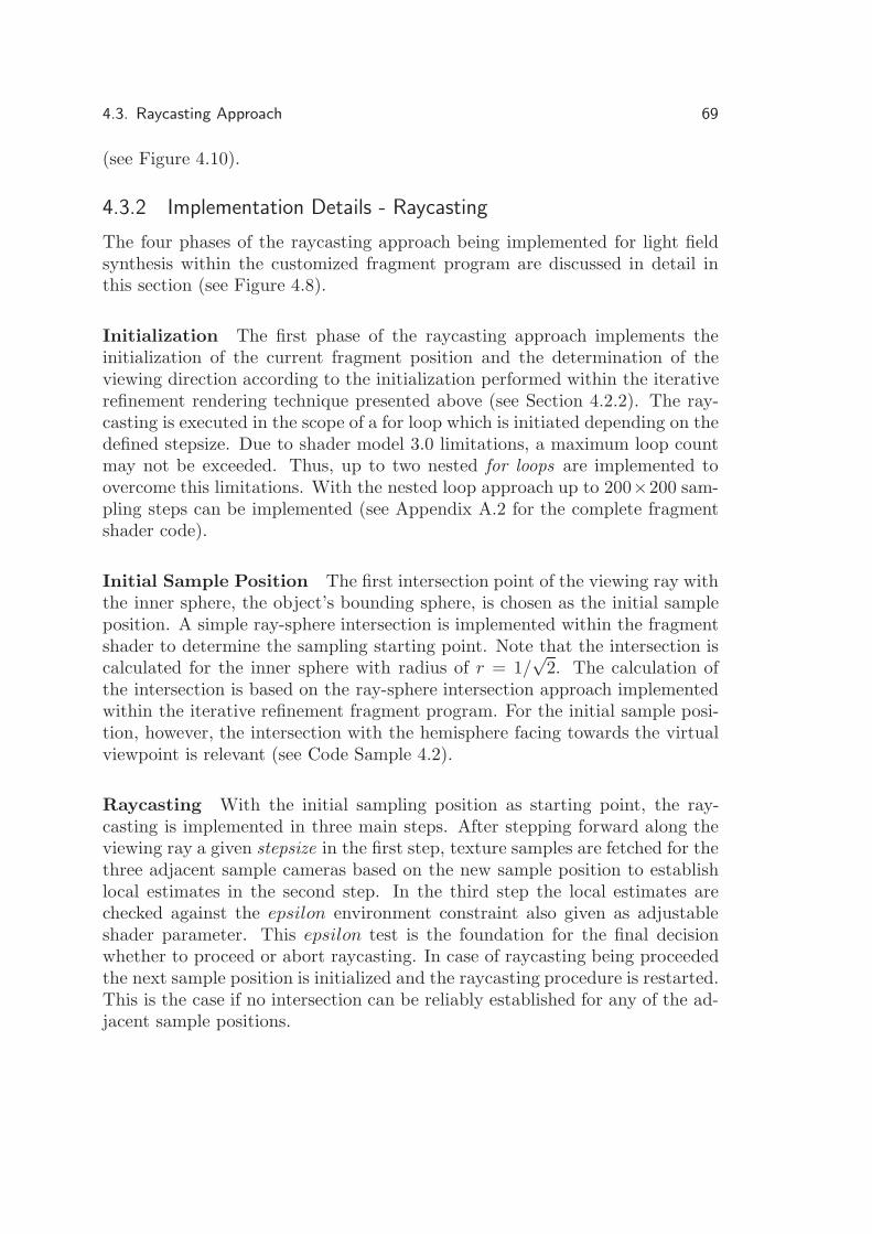
4.3. Raycasting Approach 69
(see Figure 4.10).
4.3.2 Implementation Details - Raycasting
The four phases of the raycasting approach being implemented for light fieldsynthesis within the customized fragment program are discussed in detail inthis section (see Figure 4.8).
Initialization The first phase of the raycasting approach implements theinitialization of the current fragment position and the determination of theviewing direction according to the initialization performed within the iterativerefinement rendering technique presented above (see Section 4.2.2). The ray-casting is executed in the scope of a for loop which is initiated depending on thedefined stepsize. Due to shader model 3.0 limitations, a maximum loop countmay not be exceeded. Thus, up to two nested for loops are implemented toovercome this limitations. With the nested loop approach up to 200×200 sam-pling steps can be implemented (see Appendix A.2 for the complete fragmentshader code).
Initial Sample Position The first intersection point of the viewing ray withthe inner sphere, the object’s bounding sphere, is chosen as the initial sampleposition. A simple ray-sphere intersection is implemented within the fragmentshader to determine the sampling starting point. Note that the intersection iscalculated for the inner sphere with radius of r = 1/
√2. The calculation of
the intersection is based on the ray-sphere intersection approach implementedwithin the iterative refinement fragment program. For the initial sample posi-tion, however, the intersection with the hemisphere facing towards the virtualviewpoint is relevant (see Code Sample 4.2).
Raycasting With the initial sampling position as starting point, the ray-casting is implemented in three main steps. After stepping forward along theviewing ray a given stepsize in the first step, texture samples are fetched for thethree adjacent sample cameras based on the new sample position to establishlocal estimates in the second step. In the third step the local estimates arechecked against the epsilon environment constraint also given as adjustableshader parameter. This epsilon test is the foundation for the final decisionwhether to proceed or abort raycasting. In case of raycasting being proceededthe next sample position is initialized and the raycasting procedure is restarted.This is the case if no intersection can be reliably established for any of the ad-jacent sample positions.

70 4. Spherical Light Field Rendering with Per-Pixel Depth
48 //first position on ray along view dir for first pos.49 //skip some samples if skip parameter is set50 float3 firstSamplePos = v + skip * dirN;5152 //determine intersection with inner sphere for initial skip53 //if no custom skip is given54 float skip;55 if(!skip>0.0)56 {57 float A,B,C;58 //inner sphere is of size 1.0/sqrt(2)59 C = dot(P eye,P eye) - (1.0/sqrt(2));60 B = 2.0 * dot(P eye,dir);61 A = dot(dir,dir);6263 float S = max( (B*B - 4.0 * A*C) ,0.0); //components under sqrt64 //first intersection with inner sphere neede, so take min65 skip = min( ((-B + sqrt(S)) /A/2.0), ((-B + sqrt(S)) /A/2.0));66 //take inner sphere intersection as start point67 firstSamplePos = P eye + skip * dirN;68 }
Code Sample 4.2: The initial sampling position along the viewing ray is derived fromthe ray-sphere intersection with the object’s bounding sphere if no custom skip parameteris given.
1. Update Sample Position: To update the sample position the vector tothe last known sample position is simply elongated by adding a stepsizepart of the normalized viewing direction. The new sample position isconstrained by the inner sphere. As the inner sphere limits the definedregion of valid object intersection points, all sample positions outside theinner sphere do not contribute to the final image synthesis. Thus, incase of the updated sample position being outside the inner sphere, thecurrent fragment is discarded, as the object is not visible for this pixel.
2. Determine Local Estimates: Local estimates are calculated for each ofthe adjacent sample cameras from the parabolic depth samples beingextracted based on the ray-sphere intersection of the sample camera raysthrough the current sample position. Ray-sphere intersection as well asthe parabolic texture sampling and the local estimate determination areimplemented as for the iterative procedure (see Section 4.2.2).
3. Evaluate Epsilon and Error Threshold: For the three local estimates theabsolute distances to the current viewing ray sample position are calcu-lated. In case of either one of the local estimates being closer to thesample position than defined by the epsilon parameter, the raycasting is

4.3. Raycasting Approach 71
immediately stopped. This means, that at least one camera is observingan object surface point close to the current sample position. The sam-ple cameras observing an intersection within the given threshold will beaccounted for in the final interpolation phase. In the deviant case theirinterpolation weight (cameraWeight) is reset to 0. After all, the overallinterpolation weights are normalized.
Final Interpolation With the interpolation weights of the sample camerasbeing adjusted according to the position of their local estimates with respectto the last sample position, the fragment’s final color is interpolated similarto the iterative refinement approach. Sample cameras which did not observean intersection for the last sample position do not contribute to the final re-sult. The fragment’s depth is then determined in a last step by applying themodelview-projection matrix to the last viewing ray sample position.
4.3.3 Rendering Quality - Raycasting
The raycasting rendering approach implements an efficient light field renderingtechnique that applies a precise depth correction of rays to achieve high qualityrendering results. While being less efficient by means of rendering performancecompared to the iterative refinement method, superior rendering quality isachieved. Silhouette edges and small geometric details are synthesized with ahigh precision at rendering frame rates of up to 109 fps.
In contrast to raycasting implementations being presented for renderingof displacement maps [127, 128] and relief textures [3, 83, 86], the raycastingapproach presented here benefits from multiple input depth maps to handleambiguous situations as outlined in Figure 4.6. While these related raycastingapproaches cannot handle self-occlusion and large variations in depth [7], theraycasting approach presented in this thesis precisely reconstructs the visualappearance from small structures and large geometric variations. Concavitiesand holes can be reconstructed reliably as depth information can be retrievedfrom three adjacent depth maps to determine the object intersection. Silhou-ettes and sharp edges are precisely reconstructed (See Figure 4.11).
For comparison reasons the same reference object of the Stanford Bunnyalso used to evaluate the quality of the iterative techniques was chosen todemonstrate the quality of the raycasting approach. Figure 4.11 clearly showsthe benefit of raycasting in terms of image quality compared to iterative re-finement shown in Figure 4.7. The micro and meso structures of the polyg-onal Stanford Bunny model are reconstructed from only 42 input samples asdepicted in the difference image in Figure 4.11. The difference images demon-strate the quality at the silhouette edges, small structures, and concavities.

72 4. Spherical Light Field Rendering with Per-Pixel Depth
Original geometry
42
ca
me
ras
difference x4Raycasting
64
2ca
me
ras
difference x4Raycasting
16
2ca
me
ras
difference x4Raycasting
Figure 4.11: Results of the raycasting approach at different camera sphere resolutions.Top left shows the original polygonal rendering of the Stanford Bunny model. Top rightand bottom row display the raycasting synthesis results supplemented by a differenceimage showing the pixel difference from the original geometry multiplied by a factor 4and inverted.
Good synthesis quality is achieved from a fractional amount of input samplesbeing used for iterative refinement light field rendering and related sphericallight field techniques presented in the past.
Note that the region of false pixels at the silhouette edges is diminished dra-matically compared to the silhouette errors which are appearing with the iter-ative technique being applied. Silhouettes are reconstructed precisely. Startingfrom 162 sample positions and above micro and meso structures are preciselyreconstructed. Highlights, however, cannot be reconstructed at the same highquality. For specular highlight features the raycasting approach does not showsignificantly improved rendering quality compared to the iterative approach.Thus, specular highlights exhibit the most visible differences between the orig-inal polygonal based rendering and the light field rendering.
Compared to the iterative approach per-pixel differences are significantlysmaller. The root mean square error of the raycasting approach is reducedby 40% in comparison to the iterative approach for a light field being sampledfrom 162 sample positions. However, while for the iterative approach the RMSEcould be lowered by a factor of 25% by increasing the sample amount from 162to 642, the raycasting’s RMSE is minimized by a factor of about 7% only. ThePAE remains constantly high at an error value comparable to the iterative

4.3. Raycasting Approach 73
Images MAE MSE RMSE PAE42 0,0181901 0,00530386 0,0728207 0,972241
162 0,0165208 0,00470699 0,0686075 0,960232642 0,0147035 0,00404801 0,0636240 0,947370
Table 4.3: Per-pixel color differences of the light field rendering based on varying sampledensities compared to the original rendering, showing the mean absolute error, the meansquared error, and the root mean squared error.
approach. This backups the weakness of both of the rendering approaches toprecisely reconstruct highlight effects. In total, however, the error analysisresults approve the superior quality of the raycasting approach (see Table 4.3).
4.3.4 Rendering Performance - Raycasting
The improved rendering quality of the raycasting approach comes at the cost ofreduced rendering performance. With the raycasting being applied, the overallrendering performance is reduced by about 30% compared to the iterative ap-proach. But sill, real-time frame rates are achieved for target resolutions of upto 1024 × 1024 as shown in Table 4.4. For the performance measurements thehardware and rendering setup was chosen to be identical to the iterative refine-ment performance evaluation. To achieve a rendering quality according to theresults depicted in Figure 4.11 the setting have been setup such that the stepsize was set to 0.01 and the epsilon environment was limited to 0.01. From thetable a performance drop of about 38% can be observed with each quadruplica-tion of the target 2D image resolution. Thus, the effect of the target resolutionon the rendering performance is comparable to the iterative approach. Theadditional drop in performance compared to the iterative approach is about3%. Again, the influence of the input sample image resolution is negligible inthe global view. The amount of sample positions, however, does influence theperformance to a high degree. For a target resolution of 512 × 512 as a rep-resentative set of measurements, performance is decreased by a factor of 0.58from 79.1 fps to 45.8 fps with the amount of sample positions being increasedby a factor 61 of from 42 to 2562 sample positions.
While the measurements have been performed using a high-end hardwaresetup, the raycasting algorithms also allows to perform efficiently on otherhardware platforms. With the stepsize and epsilon parameters the user canadjust the rendering performance according to his hardware capabilities. How-

74 4. Spherical Light Field Rendering with Per-Pixel Depth
Images Input Target Res. Target Res. Target Res.Res. 256 × 256 512 × 512 1024× 1024
42 256 × 256 109.79 fps 79.1 fps 49.71 fps42 512 × 512 106.23 fps 78.3 fps 44.38 fps
162 256 × 256 81.68 fps 60.4 fps 37.43 fps162 512 × 512 80.38 fps 57.8 fps 36.41 fps642 256 × 256 75.41 fps 52.1 fps 29.79 fps642 512 × 512 73.63 fps 52.2 fps 28.75 fps
2562 256 × 256 63.84 fps 46.1 fps 27.53 fps2562 512 × 512 62.29 fps 45.8 fps 26.20 fps
Table 4.4: Rendering performance for our raycasting rendering algorithm and the iterativerefinement approach applied to light fields of varying resolution with and without texturecompression.
ever, rendering speed then comes at the price of reduced rendering quality ifthe parameters are chosen to be too large. In this case discontinuity artifactsare likely to appear. Small geometric details are not recoverable with the stepsizes chosen too large.
4.4 Level of Detail for Light Field Rendering
The flexibility of the presented light field rendering techniques opens up foroptimization strategies which allow the adjustment of rendering quality to in-crease rendering performance. By adjusting the rendering quality dependingon the object’s relevance to the rendered scene, optimized performance can beachieved. With the level of detail (LOD) technique presented in this section,objects in focus are rendered at highest quality whereas distant objects arerendered at lower resolutions. The hierarchical arrangement of sample posi-tions within the spherical approximation resulting from the subdivision of theinitial icosahedron (see Section 3.3) makes the implementation of a discreteLOD strategy available for light field rendering. Additionally, the renderingtechniques open up for continously adapting the rendering performance to thequality needs for distant objects by adjusting the raycaster’s step size andintersection evaluation tolerance.
The implemented discrete LOD strategy straightly follows LOD strategiesimplemented for polygonal 3D models in interactive real-time applications. TheLOD is adjusted by coarsening the polygonal approximation being rendered for

4.4. Level of Detail for Light Field Rendering 75
light field reconstruction (see Section 4.1). Light fields being rendered with acoarser LOD are reconstructed from fewer light field probes which is in turnreducing the amount of texture switches in the rendering process and thus re-ducing the GPU workload. The spherical sample positions are arranged suchthat all of the vertices of a certain LOD are contained in the next finer LOD(see Figure 4.12). No additional spherical approximations nor additional lightfield samples have to be generated and hosted for this LOD strategy. CoarserLODs are achieved by reducing the sample density in the geometric domain byreducing the amount of sample positions. Minor popping artifacts, however,can be observed during rendering on LOD switches resulting from image infor-mation that becomes recoverable with the higher amount of sample positions,e.g. concavities. The LOD to be rendered is determined in classical sense as atradeoff of resolution vs. geometric quality. A maximum of 5 LODs (LODmax)is available assuming a highest resolution of the spherical approximation with2562 sample positions for the most detailed representation.
The discrete LOD to be rendered is determined based on the sphericalcoverage ratio (SCR) of the screen area covered by the projected light fieldbounding sphere (AS) to a the area of a full circle which perfectly fits into thecurrent viewport with the radius r being half of the shortest viewport edge.
SCR =AS
πr2(4.16)
With NLOD being a discrete LOD level and NLOD = LODmax being the finestLOD level, the LOD to be rendered is determined by
NLOD = SCR · LODmax (4.17)
As NLOD describes a discrete level the final NLOD is chosen to be the oneclosest to the result of the by the equation above.
Rendering performance can conceptionally be adapted to the object dis-tance by adjusting the render settings for the raycasting algorithm to steerthe reconstruction quality. As presented in Section 4.3.2 the precision of theraycaster is dependent on the chosen step size to sample the ray and the giventolerance at which the ray sampling is stopped. While the LOD strategy basedon the reduction of sample positions implements a discrete LOD strategy therender settings can be adjusted continuously with the object distance. A per-formance gain is achieved by increasing the raycaster’s step size. Note, however,that the epsilon parameter is to be adjusted according to the chosen stepsize.The continous level of detail offers a comfortable way of adjusting the render-ing performance. However, it was conceptually tested, only, but is not used inpractice. The discrete LOD technique on the other hand has proven to be apowerful tool for steering rendering performance and quality.

76 4. Spherical Light Field Rendering with Per-Pixel Depth
Figure 4.12: From left to right: Light field renditions of a Tie-Fighter light field (162samples at 512 × 512) rendered at varying distances and LODs with the spherical proxygeometry being superimposed. The rightmost image displays the light field rendering atmaximum rendering quality.
The LOD rendering technique is applicable to either one of the renderingapproaches presented above (See Section 4.2 and Section 4.3). The renderingperformance is steered by the object’s occupied screen space and thus showsincreased performance for distant objects, compared to a screen filled renderingof the same light field with a sample count similar to the LOD of the distantobject. The rendering quality directly corresponds to the rendering results pre-sented above, according to the number of input samples. Quality gain (shownin Figure 4.13) resulting from an increase of input samples while switching to amore detailed LOD level, however, results in noticeable popping artifacts. Fig-ure 4.13 shows the quality increase achieved by switching to a more detailedLOD.
The implementation of LOD rendering approaches results in a gain of ren-dering performance and rendering flexibility which allows light fields to beefficiently displayed. Thus, it provides an ideal solution for rendering multi-ple instances of light fields simultaneously in a dynamic scene or integratingdynamic high-quality light field renderings in complex polygonal based scenes.This technique provides a powerful tool for the flexible integration of lightfield renderings in performance critical real-time applications such as games orinteractive storytelling and educational presentations.

4.5. Progressive Light Field Rendering 77
1st LOD Level42 Samples
2nd LOD Level162 Samples
3rd LOD Level642 Samples
Difference42 vs. 162 Samples
Difference162 vs. 642 Samples
Figure 4.13: Top row: Light field renditions of a Stanford Bunny light field at differentLODs. Bottom row: Difference images showing the RGB difference of one LOD renderingto the next coarser rendition.
4.5 Progressive Light Field Rendering
Light field rendering techniques present an ideal solution to provide accessto complex data sets. The spherical light field parametrization presented inChapter 3 provides a flexible representation that allows for efficient remoteaccess and client-server based rendering methods of complex light field data.
In this section an adaption of the spherical light field raycasting approach ispresented which is optimized for web based exploration. To provide light fielddata as a web gallery, the exisiting approach would require a complete lightfield data set to be downloaded before the first image may be generated. Thus,immediate visual feedback is not available. The user is forced to wait for thecomplete data set to be downloaded and stored in client memory, even if hemight be interested in a certain view upon the data only. High quality lightfields also come with significant memory requirements for storing the necessarytexture images on the client’s local memory.
To these ends the client-server based light field rendering technique pre-sented in this section is well scalable to both the available network bandwidthand the client hardware. This approach allows light field data to be transferredprogressively on demand with respect to the interest of the client. The render-ing client automatically adapts the visual quality of the representation to theamount of host memory, and the desired run-time performance. Data that is

78 4. Spherical Light Field Rendering with Per-Pixel Depth
not required to generate an individual view will not be transferred. Thus, whiledrastically reducing data transmission, a high-quality light field rendering tech-nique is provided that makes interactive exploration of complex data availableat real-time frame rates with 6 DOF. With the proposed rendering technique,visual representations of arbitrary complex data sets can be presented in webgalleries and accessed directly.
The idea behind the progressive light field rendering technique is to replacethe static tessellation of the camera sphere (see Section 3.1) by a progressiverefinement at the client side. This will allow the client to request the imagesrequired to synthesize a particular view on demand from the server. The hier-archical nature of subdivision also allows to prioritize the requests with respectto the image quality and available client memory.
Progressive Refinement The base geometry for the local refinement is theicosahedron consisting of 12 camera positions. The cartesian coordinates of thecamera positions ci are
ci ∈⎧⎨⎩
⎛⎝ 0
±1±ϕ
⎞⎠ ,
⎛⎝ ±1
±ϕ0
⎞⎠ ,
⎛⎝ ±ϕ
0±1
⎞⎠
⎫⎬⎭ with ϕ =
1 +√
52
(4.18)
With images from these 12 camera positions which are uniformly distributed ona sphere around the object, the light field rendering approach allows for synthe-sizing virtual views from an arbitrary viewpoint at a relatively low resolution.In order to synthesize an image from one particular view point c, however, onlya few of these 12 images are required. If the virtual viewpoint c is known in thesphere’s coordinate system, the cameras ci needed to be resident in memoryfor this particular viewpoint can be easily determined by calculating the dotproducts:
if (c · ci)
{> 0 then ci is required≤ 0 then ci is not required
(4.19)
For a web-based application, these are the camera images which must be re-quested from the server. Whenever the user changes the virtual view pointc, new images must be requested (or obtained from a network cache), andpreviously transferred images may become obsolete. Figure 4.14 shows exam-ples taken from the first few steps of progressive subdivision for one particularviewing position.
To improve the overall image quality for a certain view upon the light field,additional camera positions are dynamically inserted by calculating the mid-point of each edge of the sphere tessellation and lifting the resulting vertex back

4.5. Progressive Light Field Rendering 79
Level 0 Level 1 Level 2 Level 3
Figure 4.14: The first few steps of the progressive refinement of the camera sphere. Start-ing with the icosahedron at level 0, hierarchical subdivision is performed view-dependent.
to the sphere. The sphere tessellation must then be adapted to accommodatethe newly inserted camera vertex. This way a hierarchical tessellation of thesphere is built. In order to prevent holes in the camera sphere which may resultfrom neighboring triangles of different subdivision level, two simple rules arefollowed:
1. A triangle may only be further subdivided if all of its neighbors have atleast the same subdivision level. This means that the refinement of twoneighboring triangles may not differ by more than one level.
2. If two neighboring triangles have different subdivision level, the one withthe lower level will be subdivided temporarily to prevent T-vertices fromcausing holes in the tessellation. Temporary triangles will not be furthersubdivided.
Figure 4.15 illustrates these rules: The first rule says that the green trianglesadjacent to the yellow one in Figure B may not be further refined before theyellow one is subdivided. The temporary tessellation by the second rule isshown by the dashed lines in Figure B and C. If all neighboring triangles aresubdivided as in Figure D, the temporary tessellation is replaced by a regularone. Following these rules, vertices can be easily added and removed fromthe camera sphere while still maintaining a valid view-dependent tessellationwithout any holes.
The priority of a camera request is calculated taking the virtual viewingposition in sphere coordinates (c) into account from its position ci and therefinement level si it belongs to, using a heuristic:
p(ci, si) =1sk
i
(c · ci) (4.20)

80 4. Spherical Light Field Rendering with Per-Pixel Depth
A B C D
Figure 4.15: Tessellation of the yellow triangle in dependance on the subdivision levelof its neighbors. If not all neighboring base triangles are subdivided, a temporary tri-angulation is used as indicated by the dashed lines. This will prevent holes caused byT-vertices.
The level exponent k > 0 is used to balance the progressive subdivision pro-cess. A larger value will favor breadth-first, a smaller value depth-first traver-sal. Figure 4.16 shows the influence of the level exponent k on the refinementprocess. While for k = 0.3 new cameras are inserted for the center region ofthe spherical approximation first, additional cameras in the boundary regionsof the sphere are preferred for k = 0.7. From the renderings being displayedand the additional difference images it can be seen clearly that major render-ing artifacts at the silhouette edges are improved at an early stage using thebreadth-first approach while additional details in the inner region are refinedusing the depth-first approach.
With the silhouette accuracy improving significantly with an increased sam-ple density and the the silhouette accuracy being identified to be crucial to theoverall rendering quality, a larger level exponent is conducive in most cases.With the breadth-first approach, the overall sampling density is increased whileuniformity is maintained to a certain degree within the current field of view.A level exponent of k = 0.7 has been chosen to be well suited for most webbased light field renderings as it equally supports detail refinement in the innerregions as well as silhouette accuracy.
Using the progressive refinement technique, views upon a certain sphericallight field representation are built up and are successively refined. Duringthis progressive refinement process the rendering quality continuously improvesas more detailed light field data becomes available until the final renderingquality has been achieved. Note that the final rendering quality correspondsto the rendering quality of the non progressive approaches (see Section 4.2 andSection 4.3).
Client - Server Communication The view-dependent tessellation of thecamera sphere is performed on the client side. For every newly inserted camera

4.5. Progressive Light Field Rendering 81
Original geometry
Progressive RefinementLight Field Renderingk = 0.7
Progressive RefinementLight Field Renderingk = 0.3
Diffe
rence
images
(Lig
htF
ield
vs.O
rigin
al)
Figure 4.16: Left: Rendering of the polygonal based Stanford Bunny model. Top row:Progressive rendering of the Stanford Bunny light field with a level exponent of k = 0.7.Bottom row: Progressive rendering of the Stanford Bunny light field with a level exponentof k = 0.3. Middle rows: Difference images showing the RGB difference of the progressiverendering compared to the original polygonal rendering.
position, the client sends a request for image data to the server. The server isresponsible for sending the required image and depth information to the client.A customized network protocol based on TCP has been implemented for thiscommunication. Image requests are identified by a unique hash key which iscalculated from the light field id and the requested camera position. The lightfield server maintains a hash table which refers to the hard disc location of
82 4. Spherical Light Field Rendering with Per-Pixel Depth
the image data on the server. The communication protocol is supplementedby initialization and security-related messages. The server may simultaneouslymaintain connections to different clients and different requests from a singleclient. While the rendering performance on the client side is not effected bythe server’s response, the request and update rate is effected by the serverperformance and the network bandwidth.
The client-server communication was tested in both LAN and WAN net-works. As a rule of thumb the complete network transfer of a light field willbe equivalent to transferring the same number of still images in PNG format.This holds true if the client caches all images on the local hard disc. Theimage-based remote rendering framework, however, will also work without adisc cache. In this case, images which become obsolete due to a viewpointchange will be discarded from memory and newly requested from the server ifnecessary. This allows for efficiently balancing the local memory consumptionwith the speed of interactivity and visual feedback. Figure 4.16 shows an ex-ample of the image quality during progressive transmission of the light fightfield.
4.6 Conclusion
The tradeoff of rendering speed and synthesis quality has been identified to bethe key factor to the overall performance of a light field rendering approach(see Section 1.2). The spherical light field rendering approaches with per-pixeldepth correction of rays presented in this chapter provide a comprehensive ren-dering tool set which provides a flexible and powerful solution to satisfy thischallenge. With the geometry assisted per-pixel ray interpolation best render-ing quality is achieved without noticeable ghosting artifacts at real-time framerates. Object silhouettes are reconstructed precisely and visual features frommeso and micro structures as well as concavities are reliably reconstructed. Theflexible implementation strategy provides an adjustable rendering approach bymeans of performance and quality to adapt to changing requirements.
With the iterative rendering (see Section 4.2) and the raycasting approach(see Section 4.3) two different rendering techniques have been presented. Bothof these approaches apply depth correction of rays based on the input datadirectly. Per-pixel depth information is extracted from the alpha component ofthe input samples directly to establish ray-object intersections precisely withoutthe need for complex mesh processing to be applied at runtime.
While the raycasting approach provides high-quality rendering results atmedium real-time frame rates based on sparsely sampled light fields, the itera-

4.6. Conclusion 83
tive refinement approach presented in this chapter allows for medium renderingquality at high real-time frame rates from densely sampled light fields. Thus,if memory consumption is critical and high-quality rendering results are es-sential, the raycasting approach provides the optimal solution. If, however,memory consumption is not an issue and slightly ghosting artifacts at thesilhouette edges are tolerable but rendering performance is a critical issues,the iterative refinement approach provides an alternative light field renderingsolution. Note, however, that only a fractional amount of input samples ismandatory, compared to spherical light field techniques presented in the past(see Section2.5.3), to provide sophisticated rendering results using either oneof these two approaches.
Compared to other image based rendering methods based on texture basedgeometric representations, such as displacement maps [127,128] and relief tex-tures [3,83,86], the raycasting approach provides improved ray-object intersec-tions and thus advanced rendering quality. These approaches are not capableof reconstructing complex view-dependent reflectance and geometric details re-sulting from self-occlusion, concavities and micro structures [7,83]. In compar-ison, the raycasting approach precisely reconstructs both geometry from smallstructures and large variations in depth as well as complex view-dependentsurface reflectance. It is not affected by self-occlusion or concavities.
With the LOD rendering techniques a powerful tool has been presentedwhich allows to adjust the rendering performance and quality according to theuser’s preferences and dynamic scene changes. The proposed LOD techniqueis especially suitable for complex scenes being rendered based on multiple lightfields or light fields being rendered within the context of complex dynamicscenes on a local machine.
With the progressive refinement rendering approach an alternative render-ing technique has been presented in this chapter that allows for rendering oflight fields that are not present on a user’s local machine. The progressivetechnique implements a web based rendering approach that provides remoteaccess to light field renditions stored on a remote server. Thus, this approachimplements an ideal solution for making light field data available within webbased galleries to provide access to sophisticated visualization results from avariety of sources. Such sources include the visualization of simulation datafrom earth sciences or medicine.
The rendering techniques presented in this chapter have been published bythe author to the computer graphics community in [114,117,118,120].


5
Acquisition of Spherical LightFields with Per-Pixel Depth
The spherical light field parametrization presented in Chapter 3 implements auniform sampling structure which allows high-quality image synthesis at real-time frame rates based on combined RGB and depth input samples which areencoded in RGBz parabolic texture maps. The spherical parametrization allowsfor light field reconstruction without the need for further geometry processing,neither as a pre-processing step nor within the rendering process. To fullyexploit the advantages of this light field representation within the acquisitiontask an acquisition technique should synchronously provide RGB and depthsampling capabilities in order to integrate combined RGBz samples into a lightfield representation. Optimally, the acquisition task makes use of state-of-the-art acquisition devices which provide combined RGBz images directly and athigh-update rates without costly processing. To further satisfy the demands onacquisition techniques for precision, usability and availability (see Section 1.2)the light field sampling approach should provide precise positioning abilitiesand make use of commonly available and affordable hardware devices to makea time and cost effective light field acquisition available. Acquisition approachesshould ideally assist the user in the sampling task to maximize usability. Us-ability is optimized by providing immediate visual feedback to provide a toolfor quality evaluation within the acquisition task and by guiding the user withinthe sampling device positioning process.
Unfortunately, light field acquisition techniques presented in the past donot satisfy these requirements. While with the Light Field Camera [31] andthe Plenoptic Camera [80] two flexible solutions for a hand-held acquisition oftwo-plane light fields have been presented lately, these devices are limited tothe acquisition of two-plane light field parameterizations and do not provideper-pixel depth information directly. Thus, these device do not allow for theacquisition of spherical light fields. The limitation to two-plane light field rep-resentations does not exist for acquisition setups such as the Stanford SphericalGantry [60] which are capable of moving an imaging device to any pre-defined
85

86 5. Acquisition of Spherical Light Fields with Per-Pixel Depth
sample position around an object of interest. However, the usability of such adevice is strictly limited by the financial expense, the limited portability andthe missing capability of providing geometric information directly. Acquisitiontechniques which relief the user of using complex positioning setups sample alight field from arbitrary sample positions using off-the-shelf imaging devices.Though, these approaches either rely on an unstructured light field parame-terizations which exhibit known challenges from their non uniform nature (seeSection 2.5.4) or do postulate a priori knowledge of the scene geometry in orderto re-map the captured sample to predefined sample positions. As a matterof fact, these approaches are not applicable efficiently for the acquisition ofspherical light fields with per-pixel depth.
Although per-pixel depth information is extractable from complete 4D lightfields in a post-processing step [21], a costly subsequent process is needed toextract such information. Thus, per-pixel depth information is not availablesynchronously within the acquisition phase. As a consequence these approachesare not applicable to feed combined RGBz samples to the light field represen-tation directly. Immediate visual feedback is not available for incomplete 4Dlight fields with per-pixel depth being extracted in a post-processing step.
In this chapter a flexible light field acquisition system is presented whichprovides synchronized and registered per-pixel depth and color information foreach sample at real-time. The system implements an acquisition prototypewhich makes use of state-of-the-art imaging and upcoming 3D sensor technol-ogy to acquire combined RGBz samples directly to allow for immediate visualfeedback within the acquisition process. The prototype demonstrates an effi-cient and flexible solution towards real-time acquistion of light fields which abetthe benefits of spherical light fields with per-pixel depth using future 2D/3Dimaging sensors. Precise positioning techniques are utilized to facilitate theacquisition of combined RGBz samples from pre-defined spherical positions ac-cording to the proposed spherical light field parametrization. For user guidanceimmediate visual feedback is granted for quality evaluation within the acqui-sition process and a positioning guidance system is implemented within theacquisition pipeline to ease the acquisition process.
For artificial scenes being generated from digital content using computergraphics techniques, a light field generation process is presented in this chapterwhich allows to easily generate spherical light fields from arbitrary complex syn-thetic scenes. The presented light generation easily adapts to various renderingengines and provides a sophisticated technique to extract light field represen-tations from scenes involving complex rendering techniques which are hard torender in real-time using traditional rendering approaches.

5.1. Light Field Acquisition from Physical Objects 87
5.1 Light Field Acquisition from Physical Objects
To take advantage of the benefits provided by the spherical parametrizationwith per-pixel depth, presented in Chapter 3, a light field sampling device is tobe utilized which is capable of providing registered depth and color informationon a per-pixel basis in real-time. For each light field sample to be acquired thedevice must be placed such that its position and direction corresponds to thespherical parametrization given at a certain granularity. To achieve a preciseand flexible positioning of the device, an accurate and easy to use locationsystem is to be used.
In this chapter the acquisition device and the location system of the acqui-sition process are explained in detail followed by an in depth description of theprocessing pipeline being implemented for a flexible light field acquisition inorder to acquire complete spherical light fields from physical objects.
5.1.1 Light Field Acquisition Device
For an acquisition device to be suitable for interactive acquisition of sphericallight fields it must provide reliable depth information at real-time frame rateson a per-pixel basis. The depth is to determined with per-pixel time consistencesuch that the complete image represents a static snapshot of the scene. Per-pixel depth must be synchronously available and registered with captured colorinformation.
3D Acquisition Technologies There are some technologies and algorithmsavailable for 3D scanning which may be adapted for real-time acquisition ofper-pixel depth information. These methods may be divided into active andpassive methods. While real-time passive methods based on stereo [27] or sil-houettes [71, 72] have been proposed in the past, these approaches typicallydo not perform well in the absence of scene texture and exhibit computationalcostly processing. Thus geometry reconstructions based on such passive meth-ods tend to provide instable results at low update rates.
Active methods provide more promising approaches for the interactive ac-quisition of light fields. Available active range scanning methods may bebased on time-of-flight [46, 82, 133, 134], depth from defocus [77], photomet-ric stereo [94] or projected-light triangulation [95]. Of these, the systems basedon time-of-flight may provide the most flexible techniques for light field ac-quisition. They provide full image per-pixel depth information at real-timeframe rates, expose the lowest hardware costs and especially do not demandcomputationally costly processing for geometry extraction. Recently, time-of-flight sensors have been applied in a variety of industrial contexts and have

88 5. Acquisition of Spherical Light Fields with Per-Pixel Depth
proven their effectiveness within these environments [53]. No research has beendone, however, on applying time-of-flight sensors for the acquisition of geom-etry assisted light fields. Within this thesis a prototype acquisition pipelineis implemented which makes use of a Photonic Mixing Device (PMD) time-of-flight sensor in order to interactively acquire spherical light fields with per-pixeldepth.
Photonic Mixing Device The Photonic Mixing Device (PMD) implementsan active 3D measurement device which illuminates an observed scene usingmodulated, incoherent near infrared light (NIR) (see Figure 5.1). Light beingreflected by objects within the scene is captured by pixel sensors commonlyarranged in a grid of up to 160 × 120 resolution. For each of the pixels theincoming optical signal is correlated with the internal system reference signalof the active illumination unit. For this process a sinusoidal signal is assumedas reference signal which is then correlated with the incoming signal. Thissampling is performed four times for each pixel but with an internal phase delaybeing applied. Each sampling then results in an per-pixel evaluation of thecorrelation function according to the internal phase shift. From the subsequentsampling the distance related phase shift and thus the distance to the respectiveobject region is calculated. Thus, per-pixel depth information is composedto a depth image of full sensor resolution. The sensor signal evaluation anddepth extraction is performed on the pixel sensor and the camera main boardin real-time. Signals, sampling results, and the corresponding depth valuesare accessible directly from a FireWire connection at up to 20 fps [52]. Fordetailed technological background of the PMD sensor the reader is referred toLange [54].
The PMD sensor results, however, show some artifacts resulting from theimplementation principle of this kind of technology. The distinctive features ofthe resulting data are topic of active research today. Ongoing research resultscontribute to the improvement of the PMD sensor technology and providesolutions for treatment of artifacts such as the low resolution, depth distortion,or motion blur [69].
Low Resolution Compared to up-to-date RGB imaging sensors currentlyavailable PMD sensors provide a relative small resolution of up to160 × 120. While most applications are capable of adapting to the lowresolution, the resulting large solid angle per pixel yields invalid depthvalues in areas of inhomogeneous depth occurring in situations such assilhouette edges and object boundaries. Lindner et al. have shown thatthese invalid depth values may be enhanced with an edge-enhanced dis-tance refinement approach which discards these so called Flying Pixels

5.1. Light Field Acquisition from Physical Objects 89
Incoherent IRLight Source Surface
Modulation
Phase Shift
Data
Chip with CCD Arrayand Correlation
1001001011
Figure 5.1: The time-of-flight principle of the PMD technology. Image courtesy of Kellerand Kolb [52]
concerning the sampling of sub-pixel locations while upscaling a PMDdepth image [68].
Depth Distortion As the system’s theoretically sinusoidal reference signalassumed for the correlation function is not achievable in practice, theextracted depth cannot reflect the correct distance, but comprises sys-tematic errors. This systematic error has been investigated along withstatistical uncertainties of the PMD sensor by Rapp et al. [90]. Lind-ner et al. presented an approach of the lateral and depth calibration ofsuch sensors which handles the systematic errors and statistical uncer-tainties [66, 67].
Motion Blur With the sampling of the sinusoidal correlation function de-pending on phase delay and phase shift and the sampling being performedfour times for each pixel element, the sensor is sensitive for motion. Mo-tion blur artifacts may arise in dynamic scenes since the correlation resultsof the subsequent samplings lead to varying distances regarding a pixelregion close to object boundaries.
Reflectivity The PMD sensor shows poor measurement results for two ex-treme reflectivity situations. With the infrared illumination being ab-sorbed by an object in the scene, no incoming active light is receivableby the sensor and thus the correlation function cannot be evaluated. Onthe other extreme, for infrared light being reflected perfectly, the sen-sor reaches saturation level. As a consequence, the correlation functiondoes not provide any meaningful results. While this occurs to be a spe-

90 5. Acquisition of Spherical Light Fields with Per-Pixel Depth
High Res. Color Camera
PMD CameraActive NIR Illumination
Figure 5.2: PMD camera with an additional high resolution color camera mounted.
cial burden on the PMD sensor, other measurement devices using opticalprinciples, e.g. laser scanning systems, suffer from the same problemsand do not provide more elaborate measurements in these situations.
2D/3D Camera Setup The combination of PMD depth information withhigh-resolution RGB data is in focus of current research. While Prasad etal. [88] have presented a hardware solution which combines a commodity CCDand a PMD sensor in a compact mono-ocular camera device using an opticalsplitter, this device is not available to the public yet. Todt et al. [116], how-ever, have shown that registered RGB and depth information can be capturedeffectively by combing a high-resolution RGB camera (1024×768) and a PMDcamera in a binocular setup (see Figure 5.2). While the proposed combinationdoes provide combined RGBz data on a per-pixel basis, the approach does nottake the PMD sensor characteristics into account.
Lindner et al. [70] have presented a data fusion approach which does takethe sensor characteristics into account and provides effective counter measuresto minimize the effect of PMD specific artifacts as described above. Theirdata fusion is performed in two main tasks, the distance refinement and theactual data fusion, which are arranged in a data processing pipeline accordingto Figure 5.3. Note that a simple background and invalid pixel removableis prepended to both of these tasks which discards unreliable distance valuesbased on the distinct evaluation of the four correlation function results.
Distance Refinement The distance refinement implements two optimizationsteps in order to reduce the amount of invalid pixel and thus false colormapping. First, an extrapolation of valid pixels is applied to restore

5.1. Light Field Acquisition from Physical Objects 91
PMDImage
recursive refinement
RefinedImage
Registration &Calibration Data
RGBImage
2D/3DImage
DataFusion
OcclusionDetection
BiquadraticInterpolation
Extrapolationat Boundaries
BackgroundSegmentation
Upscaling Fusion
Figure 5.3: The data fusion of PMD depth- and RGB data is performed in a processingpipeline which is conceptually split in two blocks, the distance refinement and the actualdata fusion. Image courtesy of Lindner et al. [70]
missing data for the subsequent biquadratic interpolation scheme. Theinterpolation scheme implements an upscaling of the valid region whileincorporating edge preservation. Upscaling is based on pyramidal upscal-ing [108] which recursively scales an image by a factor of two. Withthe refinement being applied, the effect of flying pixels is reduced by areasonable degree.
Data Fusion The data fusion combines both, the refined distance informa-tion and the additional high-resolution color image by back-projectingthe PMD pixels into world coordinates and a subsequent perspectiveprojection of the RGB image onto the tessellated geometric 3D repre-sentation of the PMD pixels. To avoid an RGB image undersamplingand thus a loss of information the projection is implemented based onprojective texture mapping [98]. Note that the accuracy of the fusion isstrictly dependent on the PMD depth precision and the geometric rep-resentation of the PMD pixel in 3D. Thus, the PMD device has to becalibrated first using sophisticated calibration techniques to avoid depthdistortion [66, 67]. Special care must be taken to avoid incorrect map-ping caused by occlusion effects which result from the different viewingdirections of both cameras. Here, Lindner et al. [70] provide a renderingapproach comparable to shadow maps [91,107] which reliably detects anderases occlusion effects.
Due to incoherent camera viewing frustums and the physical offset of theimage sensors, the PMD camera does not cover the same viewing volume. Thus,the PMD camera’s depth images can be mapped to a subregion of the RGBimage, only. In practice the PMD image is mapped to a region covering 77% ofthe RGB image resolution. As a consequence, combined RGBz data is availableat a maximum resolution of approximately 900 × 675 pixels. While the PMDcamera operates at a maximum frame rate of up to 20 fps, the optimization

92 5. Acquisition of Spherical Light Fields with Per-Pixel Depth
pipeline and the 2D/3D data fusion described above effect the update framerate. With the optimization being applied the update rate drops by 5 fps. Thusa maximum frame rate of 15 fps is achievable for combined RGBz images.
5.1.2 Pose Tracking
For the acquisition of light field samples an accurate position and orientationtracking system is mandatory for the sampling device. To acquire light fieldsamples from pre-defined spherical sample positions such a system must providestable and reliable tracking results with low latency to facilitate effective cameraalignment.
A selection of approaches have been presented in the past which performpose estimation based on captured input images directly and thus are not inneed of additional tracking hardware to be installed [132]. However, these ap-proaches do not provide stable tracking results for untextured scene contentsand are likely to fail in these situations. Even though advanced image basedcamera tracking approaches have been presented recently which exploit thebenefits of PMD camera devices to stabilize tracking results [10], these tech-niques exhibit computational complex and costly processing which limit theupdate rate and thus the interactive, intuitive and effective placement of asampling device.
Tracking systems which extract and exploit visible markers in the inputimages, such as the ARToolkit [45] or the Studierstube Tracker [111] have beentested for camera pose estimation. As these tracking systems are focused onoverlaying virtual imagery on real world video footage, their capabilities forcamera tracking purposes are limited. The evaluation of such marker basedsystems has shown that the accuracy of the system is highly effected by thesize and the viewing angle to the tracked visible marker [43]. thus, these systemsare not capable of reliably determining a stable camera pose. Additional tests,including multiple markers could not help to improve the tracking results. Forthis reason, an active tracking system was chosen to be best the best choice foran accurate and stable pose determination.
Active tracking systems which are in need of additional hardware compo-nents commonly attach a tracking target to the tracked device and make use ofreference signals to precisely establish the tracking target’s pose. Such systemsare commonly used in the field of Virtual Reality systems and have proven tobe well suited for interactive and accurate placement of devices. Available sys-tems exploit electro-magnetic effects, ultrasonic techniques, or optical systemsfor pose estimation.
Electro-magnetic systems [5] exploit the effects of electro-magnetism to de-termine the pose of a tracking target within the magnetic field. These ap-

5.1. Light Field Acquisition from Physical Objects 93
proaches are subject to ferromagnetic interferences and are thus unsuitable forthe positioning of a camera covered by metal and attached to a power cord.
Acoustic tracking systems [51], either exploit the time-of-flight or the phasecoherence of an ultrasonic signal, to determine the distance and orientationof a receiver relative to a transmitter. Due to the nature of sound acoustic,tracking is relatively slow and effected by temperature, air pressure or changesof the humidity as these aspects effect the speed of sound. These systems showpoor positing results for environments which exhibit reverberation and echo.
Optical tracking systems [85] make use of infrared based illumination andcamera systems to establish reliable and stable pose estimation. With the mea-surement volume being lit by infrared light sources the reflection of a trackedmarker is captured by multiple cameras. For each camera the line of sight tothe marker is established and from the intersection points of these lines the3D position is established (see Figure 5.4). Using multiple markers in a fixedsetup, the setup’s pose is determinable with 6 DOF. Though, special care mustbe taken in the setup of such a system to avoid occlusion and ensure visibilityof a target in the complete measurement volume from at least two camera pos-tions. While these systems provide a precise, flexible and stable solution for thepositioning task within the light field acquisition process, it must be mentionedthat the benefits come at increased financial costs, starting at 12.000 EUR fora portable four camera system. But still, these costs make up only a fractionalpart of compared to prices which must be calculated for gantry based position-ing systems such as the Stanford Light Field Gantry and are comparable tothe prices for acoustic or electro-magnetic tracking systems. Compared to theacoustic and electro-magnetic systems, however, the optical tracking system isless effected by any environmental interferences.
Optical Camera Tracking The DTrack optical camera tracking system im-plements a high-end tracking system for 3D and 6D tracking of custom trackingtargets [4]. The system consists of a PC workstation, two or more trackingcameras, and up to 20 custom tracking targets. The PC workstation runs thetracking software which calculates the 6 DOF target positions and orienta-tions within the tracking volume from the line of sight to the marker’s infraredreflection which is captured in 2D by the cameras (see Figure 5.4). The intelli-gent tracking cameras are equipped with an FPGA for accelerated marker dataanalysis. The cameras also include an infrared flash to illuminate the trackedobjects. Up to 16 cameras can be combined in a tracking system. 3D Mark-ers and 6D Targets can be calibrated for the tracking system and mounted toany custom device. Tracking is performed at an update rate of 60 Hz with amaximum error of 0.5 mm in position and 0.1◦ in orientation.

94 5. Acquisition of Spherical Light Fields with Per-Pixel Depth
2D data fromcamera
2D data fromcamera
3D / 6DOutput data
IR flash fromtracking camera
IR flash fromtracking camera
reflected IRlight
calculatedoptical ray
calculatedoptical ray
Figure 5.4: Optical tracking principle. The 2D image position of the IR reflectionscaptured by the cameras are utilized to determine 3D positions of single markers and thepose of tracking targets with 6 DOF. Image courtesy of A.R.T. GmbH [4]
Tracking Setup For tracking the position and orientation of the bifocal PMDcamera setup a 6D tracking target consisting of five reflective 3D mark-ers is mounted on top of the RGB camera. To ensure visibility for anappropriate tracking volume four ARTrack2 cameras have been installedto the ceiling of a laboratory environment such that a tracking volumeof 5 m × 3 m × 3 m is reliably covered. Note that extensive tests havebeen performed to evaluate the influence of the tracking system’s infraredflashing system on the PMD sensor system. Fortunately an effect of thetracking system’s flash on the PMD sensor precision could not be di-agnosed. A stationary system has been utilized in this case. However,portable systems are also available for more flexible application areas.
Hand-Eye Transformation With the 6D tracking target mounted to thecamera system the target’s pose is reliably determinable in tracking co-ordinates. However, the pose of the RGB camera sensor not the trackingtarget’s pose is relevant as reference value to steer the light field acqui-sition process. Thus, the fixed transformation from the tracked targetcoordinate system to the camera coordinate system is essential for theacquisition process. The determination of this transformation is calledthe hand-eye calibration problem and got its name from the robotics com-munity, where a camera (eye) is mounted to the end effector (hand) of arobot. In this context several approaches have been presented in the past

5.1. Light Field Acquisition from Physical Objects 95
no
yes
2D/3D CamCapture combinedRGBz images
Pose TrackingTrack image sensorpose
3D MeshingGenerate 3D meshfrom RGBz imagebased on intrinsic andextrinsic cameraparameters
Cameraat desired sample
position?
ParabolicMappingRender meshwith sample camerasettings and acquireparabolic map
Light FieldRenderingVisualize currentlight field state
Update LightField DataAdd current sampleto light field re-presentation
Figure 5.5: The light field acquisition pipeline: From the captured RGBz image a 3Dmesh is generated according to the camera’s intrinsic and extrinsic camera parameters.If the camera is positioned according to a pre-defined spherical sample position then the3D mesh is rebinned to the sample position and a parabolic RGBz map is generated andstored with the light field representation.
to solve this problem using a calibration pattern [56, 121, 122]. RecentlyStrobl and Hirzinger have presented a new calibration pattern based ap-proach [109] which is available as a free software toolbox [110]. Thetoolbox takes a series of calibration pattern images and 6D tracking tar-get poses to extract the desired hand-eye calibration. Using the providedtoolbox the hand-eye transformation is determined efficiently. Applyingthe hand-eye transformation to the tracking results yields the imagingsensor pose in the tracking system’s coordinate system directly.
5.1.3 Light Field Acquisition Pipeline
With the 2D/3D RGB-PMD camera setup and the accurate pose tracking sys-tem, the critical hardware components are available to establish an efficientlight field acquisition process. The acquisition process presented in this sec-tion is implemented as a processing pipeline taking the RGBz images of the2D/3D camera setup and the tracked camera pose as input data. Based onthis input data the light field is sampled from pre-defined positions. Capturedlight field samples are fed into the spherical light field representation and the(incomplete) light field is being rendered directly and continuously for imme-diate visual feedback and quality evaluation. See Figure 5.5 for an overviewof the processing pipeline. The pipeline can be structured in five subsequent
96 5. Acquisition of Spherical Light Fields with Per-Pixel Depth
steps. After updating the input data, a 3D polygonal mesh is reconstructedfrom the RGBz data. The camera’s pose is evaluated against the pre-definedspherical light field positions and a light field sample is acquired if the camerapose does correspond to a specific sample position. With a light field samplebeing acquired, the light field representation is updated and the preliminarylight field is rendered.
Input Data Update The input data is updated by synchronously pollingnew data from both, the 2D/3D camera setup and the DTrack tracking system.When polling new data from the camera setup, the sensor data of the RGB andthe PMD camera are read out and fed into the PMD processing and 2D/3Dfusion pipeline as described in Section 5.1.1. The PMD pipeline implementsstate-of-the-art optimization and correction functions based on specific PMDcharacteristics and thus provides optimized RGBz data at a frame rate of 15 fps(see Section 5.1.1). The image senor’s pose is updated based on the tracking re-sults by applying the hand-eye transformation. Thus, the update step providesthe 2D/3D camera’s fusionated RGBz image and the current camera setup’spose in tracking coordinates.
3D Mesh Generation From the actual camera setup’s pose and the RGBzimage data a 3D polygonal mesh is reconstructed based on the intrinsic cameraparameters which are available from the PMD processing pipeline described inSection 5.1.1. The mesh is generated first in the camera coordinate system withthe image sensor being the origin and the negative z-axis pointing in cameraviewing direction. Then, with the tracked pose and the hand-eye transforma-tion matrix to be known, the mesh is transformed to the tracking coordinatesystem by applying the tracking transformation matrix and the hand-eye trans-formation matrix. For clarity and simplicity reasons in this chapter the trackingcoordinate system is defined to be identical to the world coordinate system.
Initial Triangle Mesh To generate a 3D mesh from the RGBz images a tri-angle mesh is rendered using a vertex buffer object. The vertex bufferobject is initialized once as a triangle mesh with a resolution equal to theinput camera resolution, such that the centers of four adjacent camerapixels are connected by the edges of a quad and the quad being split intotwo triangles. The mesh is generated in normalized device coordinates(NDC) and a z value of 0 such that it equally spans along the x and y di-rection in the range of [-1,1]. The updated input RGBz image is mappedto the triangle mesh as texture with the alpha component containing thedepth values. The depth values are interpreted as offset values. The

5.1. Light Field Acquisition from Physical Objects 97
mesh is rendered using a customized geometry- and fragment program.While the fragment program performs a simple texture mapping opera-tion only, the geometry shader implements the mesh reconstruction andoptimization process.
Within the geometry shader the depth values are fetched from the alphachannel of the input textures. The depth values are then applied to thevertices as offset values in the z component. Thus, from the input meshbeing defined with vertex coordinates V = (x, y, 0)T and x, y ∈ [−1, 1] anoffset mesh is generated. The offset mesh expands orthogonal to the X/Yplane in the negative z direction. Note that the depth values are givenas radial depth values along per-pixel rays in the 2D/3D camera setup.While the x and y components of the mesh are defined in the camera’snormalized device coordinates, the depth values now need to be convertedto NDC in order to achieve a consistent representation. This can be easilydone by projecting the vertices to the camera image space using thecamera projection matric (MCProj ). The projection matrix is extractedfrom the intrinsic camera calibration parameters which are known fromthe PMD processing pipeline. Note, however, that only the z componentis to be adjusted. Thus, for a given mesh vertex VOffset(x, y, z) onlythe z component is substituted by the projected z component of vertexVProj .
VProj = (xProj , yProj, zProj)T = MCProj · VOffset (5.1)
With the z value being substituted the adjusted verticesVNDC(x, y, zProj)T now define the mesh in NDC.
From the structure of a regular projection matrix it can be easily seenthat the z component of the projected vertex is computed independentlyof the x and y components. Thus z values (depth values) can be handledand transformed to NDC independently (see Moller and Haines, pp 61–66 [2]).
To finally render the mesh in cartesian camera coordinates the mesh isunprojected again using the inverse camera projection matrix (M−1
CProj).
Then the VNDC are transformed to camera coordinates VCam accordingto:
VCam = (xCam, yCam, zCam)T = M−1CProj
· VNDC (5.2)
Mesh Optimization In this stage the triangle mesh represents a solid surfacein camera coordinates. For boundary regions occurring at sharp edges

98 5. Acquisition of Spherical Light Fields with Per-Pixel Depth
RGBz Input Image Triangle Mesh reconstruction
Clipping Planes
Gradient Culling
Isolated Object Mesh
Figure 5.6: Top Left: Based on RGBz input images polled from the light field acquisitiondevice at a resolution of 900 × 675 pixels (see Section 5.1.1), a triangle mesh is recon-structed in camera coordinates. Top, middle: Elongated triangles resulting from depthinterpolation at boundary edges are visible for viewing directions which diverge from thecurrent 2D/3D camera setup pose. Top, right: Reconstruction artifacts are erased byapplying a gradient based triangle culling. Bottom, right: Redundant geometric detailsare culled by adjusting up to 6 clip planes to isolate the object of interest.
within the observed object or at the silhouette edges, reconstructed tri-angles span over a large variation in depth. These triangles occur inregions which are occluded from the camera’s point of view and thus donot provide exploitable depth values. If observed from a position beingexactly identical to the input camera’s pose, these triangles are not visi-ble as they span in line of sight. For slightly varying viewing directions,however, these triangles occur as extremely elongated textured triangles(See Figure 5.6, top middle). As these regions are not visible from theoriginal view, the texture does not carry any meaningful information andthe shape, resulting from the interpolation of adjacent depth values, canbe interpreted as reconstruction artifact. Fortunately, these regions are
5.1. Light Field Acquisition from Physical Objects 99
identified easily by evaluating the gradient for each vertex based on dis-crete depth values using finite difference methods within a given triangle.A triangle is culled within the geometry shader, if the gradient exceedsa given threshold value which is defined by the user (see Figure 5.6, topright).
For scenes also including regions of non-interest such as background de-tails and additional information to the sides of the object of interest, clipplanes are implemented to provide a flexible tool for object isolation. Upto six clip planes are available which are aligned along the camera coor-dinate axis and alow to cull 3D content by limiting the maximum andminimum x,y and z values of the reconstructed mesh vertices (see Fig-ure 5.6, bottom right). Note, however, that the clipping planes as well asthe threshold value being used for the gradient based culling of trianglesare to be adjusted manually with every light field sample to be acquiredto ensure best acquisition results.
With the mesh optimization being performed, an isolated solid surfacemesh of the captured object is rendered in camera coordinates. By apply-ing the tracking and hand-eye transformation this mesh is easily trans-formed to the tracking coordinate system.
Camera Pose Evaluation With each update circle of the light field acquisi-tion pipeline, the camera setup’s pose is evaluated based on the tracking resultsand compared against the pre-defined set of spherical sample positions. Re-member that the sample positions are defined by the spherical approximationgiven by the light field parametrization (see Section 3.1). Thus, given a specificsample resolution of 12, 42, 162 or 642 sample positions, discrete sample posi-tions are pre-defined. Tracking coordinates are evaluated in meters. Thus, theunit sphere is defined with a radius of 1 m centered at the origin of the trackingcoordinate system. With the sample positions to be known, the current 2D/3Dcamera position and central viewing direction can be evaluated with respectto these positions. Note, however, that the spherical representation and thecamera position must be defined with respect to the same coordinate system.For clarity reason, the spherical representation and the 2D/3D camera pose areassumed to be given with respect to the tracking coordinate system. Note thatdifferent base coordinate systems can be easily defined by applying a commoncoordinate system transformation to both, the spherical sample coordinatesand the tracked camera coordinates.
In the ideal case, the camera is positioned such that the position is iden-tical to a spherical sample position and the camera’s viewing direction doescorrespond to the central sampling direction. The central sampling direction is
100 5. Acquisition of Spherical Light Fields with Per-Pixel Depth
given by the vector emerging from the sample position and passing through thespherical representation’s origin, in this case, the tracking coordinate system’sorigin. However, positioning the camera according to a sample position and -direction is a challenging task. Thus, for user convenience the pose is evaluatedwith a certain tolerance.
While defining an epsilon environment around a desired sample positionwould provide a straight forward solution for a ”soft” pose evaluation, thisapproach does not take the viewing direction into account. Thus, two distinctepsilon environments have been implemented for each, the camera’s directionand its position. To evaluate the camera’s pose, the closest sample positionis determined first. The closest sample position is determined efficiently byintersecting the ray, emerging from the origin and passing through the cameraposition, with the spherical approximation. Based on the hierarchical structureof the spherical approximation, a single triangle which is intersected by this rayis identified quickly by establishing the intersection with the sparsest sphericalapproximation and then subsequently refining the intersection based on thetriangles of the next finer discretization level. The closest sample position isdetermined from the corresponding three vertices (see Figure 5.7, left). Forthe closest sample position the direction is evaluated first. If the difference inthe camera’s central viewing direction and the sample position’s central sampledirection (εα) does not exceed a given epsilon angle the camera’s orientationis assumed to be valid. In a second step the camera’s absolute distance to thesample position is evaluated. The camera’s pose is assumed to be valid if thedistance (εd) does not exceed a given epsilon distance (see Figure 5.7, middle).
However, under certain circumstances the user might not be able to movethe camera along a path on the spherical approximation’s surface. Thus, forsome reasons he might be limited to setup the camera such that the camerapose does fulfill the directional constraint but fails the distance constraint.In these cases the camera pose is still considered to be valid as long as thecamera’s central viewing ray does intersect the spherical approximation withinthe given epsilon distance environment. As shown in Figure 5.7, right, thecentral viewing ray does still correspond the sample position’s central viewingdirection in these cases and thus provides valid information. Sampling rays tothe sides of the central direction, however, exhibit an increasing angular error.The angular effect is factored by the camera’s distance to the sample position.While providing a more flexible camera positioning approach, this flexibilitycomes at the price of directional error to the sides of the central samplingdirection. Thus, it is to used under exceptional circumstances, only.
For user guidance a graphical representation showing the spherical approx-

5.1. Light Field Acquisition from Physical Objects 101
Figure 5.7: The camera’s central viewing direction and its position is evaluated with re-spect to the closest sample direction. Left: Central camera viewing direction within giventolerance (εα), but the camera fails the positional constraint. Middle: Camera withinepsilon environment of both, direction and position. Right: The directional constraint isfulfilled and the camera’s viewing ray intersects the spherical approximation within thepositional epsilon environment but the camera itself is not positioned within the epsilonenvironment. Note that the camera’s central ray corresponds to the central samplingdirection, while rising angular errors occur for divergent directions.
imation and a proxy geometry of the camera setup with the camera’s field ofview is available during the acquisition task. The closest sample position andthe epsilon environment are being highlighted.
Parabolic Mapping and Sample Acquisition With the 2D/3D camerasetup being placed according to a pre-defined sample position and the ob-served object mesh being reconstructed, a light field sample can be acquiredby parabolically mapping the mesh from the pre-defined sampling position onthe unit sphere.
Depending on the object from which a light field is to be acquired, theobject does not necessarily fit into this representation. Remember, the object’sbounding sphere has to be defined such that it is centered around the origin witha radius of 1√
2(see Section 3.2). Hence, for objects exceeding the dimensions of
the unit sphere the reconstructed mesh has to be scaled to fit into the boundingsphere. Obviously, if a scaling is applied to the mesh for one sample position, ithas to be scaled accordingly for all of the sample positions to maintain constantproportions.
Then, to acquire a light field sample according to the parabolic image spaceparametrization, the standard vertex processing step being implemented for themesh reconstruction is replaced by a customized vertex program, which projectsall vertices onto the unit sphere and converts the result to parabolic coordinates.For the generation of parabolic coordinates it is essential to transform the scenesuch that the sample capture position is placed at C = (0, 0, 1)T , looking alongthe negative z-axis. Thus, the scene is transformed according to the sample

102 5. Acquisition of Spherical Light Fields with Per-Pixel Depth
position’s viewing matrix which is obtained from the spherical parametrizationfor the current sample position.
The steps performed by the customized vertex program comprise the fol-lowing.
1. Projection to the hemisphereEach mesh vertex V is projected from the sample point onto the oppositeunit hemisphere. The projection is computed by casting a ray from thesample position through the vertex and intersecting this ray with the unitsphere. This amounts to solving a simple quadratic equation and resultsin a projected vertex S.
2. Parabolic mapping of the projected verticesAs a result of the previous step, the projected vertex S is lying on thehemisphere with z < 0. The vertex S is then converted to paraboliccoordinates, according to Equation 4.2
3. Depth AdjustmentThe depth value is calculated as the fractional part of the secant lengthaccording to Figure 3.6.
Based on this parabolic mapping, light field samples are acquired from thereconstructed mesh being generated based on the 2D/3D input images of thecamera setup being positioned at the sampling position. However, accuratelight field samples are achievable only, if the camera is placed exactly corre-sponding to the position and direction pre-defined by the spherical represen-tation. As mentioned above, an epsilon offset has been implemented for userconvenience in the positioning task.
In case of the camera being set up such that its central viewing directiondoes differ by some degrees, the reconstructed mesh does exhibit visible recon-struction artifacts when being rendered from the pre-defined sample position(see above: 3D Mesh Generation - Mesh Optimization). Without mesh opti-mization being applied this results in geometric details being visible which arenot visible from the 2D/3D camera’s point of view and thus do not containvalid information. With the mesh optimization being applied, theses artifactsare removed. In this case, no information is visible in these undefined regions.Thus, with a light field sample being acquired from slightly varying samplepositions this will result in no light field information being available for theseregions. However, in the reverse this will avoid misleading information to beintegrated into the light field representation. As up to three input light fieldsamples are evaluated within the light field rendering process (see Section 4.1)missing information in one of the light field samples will likely to be coveredby one of the two other light field samples.

5.1. Light Field Acquisition from Physical Objects 103
Note, however, that in addition to mesh reconstruction artifacts, the 3Dmesh does not represent the scene’s correct reflectance characteristics if thevariation in direction and position is chosen too large. Thus, the epsilon en-vironment is to be chosen small to avoid dubious information being sampled.In practice an angular epsilon environment of 0.5◦ − 1◦ for the maximum di-rectional deviation and a corresponding maximum positional error of (8 mm- 15 mm) have proven to result in both, a convenient acquisition process andacquisition results which do not exhibit artifacts resulting from reconstructionartifacts as described above.
While this acquisition approach is targeted at the acquisition of light fieldsamples from pre-defined spherical sample positions, it involves some manualinteraction to achieve reliable results. The gradient threshold being utilized fortriangle culling and the clipping planes have to be adjusted manually for everysingle light field sample. Special effort has to be spent to position the RGBzlight field acquisition device according to the pre-defined sample position. How-ever, following this strict acquisition process guarantees a uniform acquisitionand representation of a spherical light field. Thus, the acquisition process isstrictly driven by the underlaying spherical light field parametrization.
Different acquisition approaches which allow for a more flexible acquisitionby adjusting the spherical light field parametrization depending on a freelychosen camera pose have been evaluated but could not provide satisfactoryresults. Comparable to free form light fields and unstructured lumigraphs, theseapproaches make the parametrization dependent on the acquisition process.Thus, the quality of the parametrization and as a consequence the quality of thesuccessive light field synthesis is driven by the acquisition process. The benefitsof a uniform parametrization are lost, as uniformity cannot be guaranteed withfreely chosen camera positions. For this reason, these acquisition approacheshave not been implemented as a solution to the acquisition task in this work.
Light Field Update and Rendering The light field sample being acquiredin the previous step is integrated into the spherical light field representationdirectly without further processing. With the first sample being acquired, thelight field renderer is capable of providing synthesized images based on thecurrent set of acquired samples at real-time to provide a visual representationfor quality evaluation within the acquisition process.
Thus, while acquiring additional samples, the user is capable of evaluatingthe current light field quality. Improper light field samples can be removedfrom the representation and replaced by new samples to maximize the qualityof an acquired light field.
In practice, this accompanying visualization has proven to be a powerful

104 5. Acquisition of Spherical Light Fields with Per-Pixel Depth
A B C D
Figure 5.8: Light field acquisition results of a stuffed animal which exhibits diffusematerials only. A: The input RGB image showing the animal with background. B: RGBimage with the background being keyed out. C: Rendering of the light field being acquiredfrom 162 sample positions at a resolution of 512×512. D: Difference image showing per-pixel differences of the light field rendering (C) and the input RGB image (B) multipliedby a factor of 4 and inverted.
tool for quality evaluation and visual guidance to optimize acquisition results.
5.1.4 Acquisition Results
With the 2D/3D sampling hardware, the tracking system and the proposedlight field acquisition pipeline, light fields can be efficiently sampled from phys-ical objects. The proposed acquisition reveals the potential of the bifocal PMDcamera setup for the acquisition of light fields with per-pixel depth. However,the results expose limitations which are reasoned in the systematic and thecurrent development state of the young PMD technology.
Figure 5.8 shows light field acquisition results for a light field being capturedfrom a stuffed animal. The physical object features a compact structure anddiffuse materials. Thus, the object does not exhibit large variations in depthand practically no sharp boundary edges in the inner region. The silhouetteedges, however, provide boundary regions with abrupt and large depth variationwith respect to the background. The object’s fur does exhibit diffuse materialproperties and thus provides uniform reflections. Regions which are covered bylight absorbing materials or reflective materials do not occur.
In Figure 5.8 an RGB image of the stuffed animal (Figure 5.8, A) is shownaccompanied by the rendering of the light field (Figure 5.8, C) being acquiredusing the 2D/3D PMD camera setup. A difference image showing the inverseper-pixel differences multiplied by a factor of 4 is shown in Figure 5.8, D. Forcomparison reasons the original input RGB input image is displayed with thebackground being keyed out (Figure 5.8, B).

5.1. Light Field Acquisition from Physical Objects 105
Figure 5.9: Light field being captured from Christof Rezk Salama. Discontinuity artifactsappear in regions of infrared light being absorbed during acquisition. Left: RGB inputimage with the background being culled. Middle and Right: Light field rendering withthe discontinuity artifacts being highlighted in the bottom row.
From the difference image it can be seen clearly that the inner regions of theobject are reliably captured and reconstructed. Some minor artifacts occur atthe image contours such as the nose, the hands or the feet. Solely the silhouetteexhibits some more visible artifacts which occur as aliasing like rendering ar-tifacts. These visible stepping artifacts result from the PMD camera’s relativelow resolution of 160× 120 and the resulting large solid angle. The large solidangle yields invalid depth values in areas of inhomogeneous depth occurring insituations such as silhouette edges and object boundaries (see Section 5.1.1).With these invalid regions being culled within the acquisition process, theseregions are not present in the light field representation and thus cannot bereconstructed in the image synthesis. As a consequence, the mean absoluteerror of per-pixel color values resulting from the comparison of the input imageand the rendered result is reasonable high (0.0678861). The root mean squarederror for the same pair of images is determined accordingly high (0.209604).
While the stuffed animal did provide diffuse materials, only, additional ar-tifacts arise from light absorbing materials. Figure 5.9 demonstrates the effect

106 5. Acquisition of Spherical Light Fields with Per-Pixel Depth
of infrared light being absorbed within the acquisition. Per-pixel depth cannotbe evaluated reliably with the infrared light being absorbed in some image re-gions. Thus, the polygonal mesh being reconstructed for the sampling processis built from incorrect and incoherent depth information in these regions. Thesegeometric artifacts are sampled within the acquisition process and appear asdiscontinuities within the light field synthesis process. Figure 5.9 displays theresults of a light field being acquired from Christof Rezk Salama. The lightfield renderings clearly demonstrate the effect of light being absorbed by theblack hair. For this region heavy discontinuity artifacts appear.
However, the rendering results displayed in Figure 5.9 also show the strengthof the presented approach. Note that ghosting artifacts are minimized to areasonable amount. While some ghosting artifacts occur in the face region, theshirt’s printing is reconstructed without noticeable artifacts.
For complex scenes covering large variations in depth, which exhibit allvariations of materials and expose sharp boundary edges, the proposed acqui-sition approach is effected by the PMD setup’s limitations to a high degree.Figure 5.10 shows the acquisition results of such a scene. Infrared light absorb-ing materials (labeled A in Figure 5.10) occur as holes or exhibit discontinuityartifacts in the light field rendering. High reflective material causes the PMDsensor to reach saturation level in the acquisition process if infrared light isperfectly reflected. Thus, no valid depth information and as a consequence nogeometric detail is available for these regions. These regions are not acquiredand appear as holes (labeled B) in the rendering.
For this kind of complex scenes being composed from multiple objects,ghosting and geometric distortion effects appear at boundary edges (labeledC). For the boundary edges depth information cannot be reliably reconstructed.Due to the PMD camera’s large per-pixel solid angle, the depth informationbeing acquired for these regions results from a mixture of values being mea-sured for different object surface distances. For small variations in depth thegradient threshold being applied for mesh optimization within the acquisitionprocess does not suffice as a counter measure. This results in geometric dis-tortions being acquired and reconstructed within the light field synthesis. If,however, the gradient threshold is chosen too small, discontinuities and loss ofgeometric information may appear in region of boundary edges (labeled D).As this complex scene is composed from a selection of relatively small objects,the silhouette artifacts effect the overall quality of the light field rendering toa high degree.
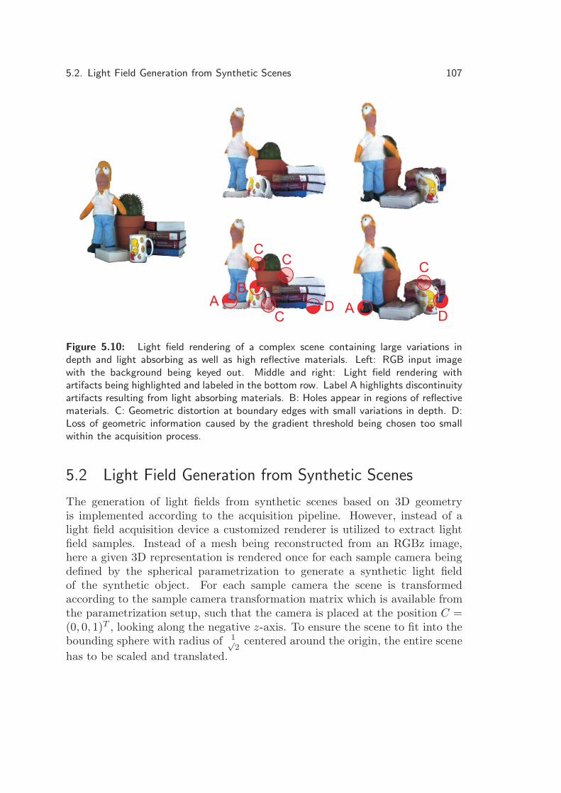
5.2. Light Field Generation from Synthetic Scenes 107
AA
C
CC
B
DDC
Figure 5.10: Light field rendering of a complex scene containing large variations indepth and light absorbing as well as high reflective materials. Left: RGB input imagewith the background being keyed out. Middle and right: Light field rendering withartifacts being highlighted and labeled in the bottom row. Label A highlights discontinuityartifacts resulting from light absorbing materials. B: Holes appear in regions of reflectivematerials. C: Geometric distortion at boundary edges with small variations in depth. D:Loss of geometric information caused by the gradient threshold being chosen too smallwithin the acquisition process.
5.2 Light Field Generation from Synthetic Scenes
The generation of light fields from synthetic scenes based on 3D geometryis implemented according to the acquisition pipeline. However, instead of alight field acquisition device a customized renderer is utilized to extract lightfield samples. Instead of a mesh being reconstructed from an RGBz image,here a given 3D representation is rendered once for each sample camera beingdefined by the spherical parametrization to generate a synthetic light fieldof the synthetic object. For each sample camera the scene is transformedaccording to the sample camera transformation matrix which is available fromthe parametrization setup, such that the camera is placed at the position C =(0, 0, 1)T , looking along the negative z-axis. To ensure the scene to fit into thebounding sphere with radius of 1√
2centered around the origin, the entire scene
has to be scaled and translated.

108 5. Acquisition of Spherical Light Fields with Per-Pixel Depth
Note, that this procedure is conceptually identical to the acquisition ap-proach being utilized to sample a light field from the reconstructed 3D meshof a physical object (see Section 5.1.3). Thus, the same customized vertex pro-gram is utilized to project all vertices onto the unit sphere and to convert theresult to parabolic coordinates. This allows for the efficient generation of syn-thetic light fields using commodity graphics hardware. Due to the non-lineargeometric distortions resulting from the parabolic mapping applied by our ver-tex program, however, it is mandatory to tessellate coarse geometry into smalltriangles before light field synthesis. On modern graphics hardware this canefficiently be achieved by a geometry shader program.
Arbitrary complex fragment programs can be used in combination withthis customized vertex program. The only modification necessary is that thefragment program must write the interpolated depth value generated by thevertex shader into the alpha portion of the final color.
Each parabolic map is stored as an interleaved array of RGBz values. Indi-vidual parabolic maps are associated with the sample position’s transformationmatrix defined by the spherical parameterisation.
For usability reasons the light field generation algorithm was integratedinto commercially available 3D modeling packages like Autodesk Maya whichare commonly used in the computer graphics community. Using the plug-in, light fields can be generated efficiently from arbitrary complex 3D objectscontaining sophisticated material and (global) illumination effects. For lightfield generation any render engine available with the 3D modeling package canbe applied.
All of the light fields being used to demonstrate the quality of the lightfield rendering approach have been generated from synthetic objects using thisproposed technique (see Section 4.1). Light fields of the Tie-Fighter model(see Figure 4.12) an Michelangelo’s David statue (see Figure 6.1) have beengenerated using the Autodesk Maya plugin.
5.3 Conclusion
Within this chapter two approaches have been presented to generate sphericallight fields with per-pixel depth. While the first approach exploits upcomingdepth imaging sensor technology in combination with sophisticated trackingtechnology to acquire light fields from physical objects, the second approach isaiming at the generation of light fields from synthetic objects.
For synthetic objects spherical light field representations can be generatedautomatically from any given synthetic 3D representation using a specialized
5.3. Conclusion 109
rendering engine. The integration of light field generation capabilities intocommercially available 3D modeling packages provides a powerful tool for theflexible generation of sophisticated light fields from any kind of synthetic ob-jects. Light fields being generated from synthetic objects provide high qualityrepresentations which are reconstructed precisely using the raycasting light fieldrendering approach presented in Section 4.3.
For physical objects an acquisition approach has been presented which im-plements a prototype setup for the interactive acquisition of spherical lightfields. The approach makes use of a bifocal 2D/3D camera setup built from aPMD time-of-flight depth imaging sensor and a high resolution RGB camerato acquire combined RGBz information directly without the need for addi-tional processing to extract per-pixel depth information. From the combinedRGBz images a polygonal 3D mesh can be reconstructed in world coordinatesefficiently using a high precision optical tracking system. With the 2D/3Dcamera being adjusted according to a pre-defined sample position, a light fieldsample is easily acquired by rendering the 3D mesh from the sample position.
While state-of-the-art optimization techniques have been implemented tooptimize the PMD sensor performance, light field acquisition is still effectedby the sensor characteristic to a high degree. The physical object acquisitionresults demonstrate the main shortcomings of the 2D/3D PMD camera sys-tem. Due to the low resolution of the PMD camera boundary edges cannot beacquired precisely, leading to discontinuity and distortion artifacts in the meshreconstruction and thus in the light field representation. The acquisition islimited to scenes which do not exhibit materials that absorb near infrared lightand do not provide high reflective materials. In appearance of one of those ma-terials, the PMD sensor will provide unreliable depth information which effectsthe mesh representation to a high degree. Thus, the acquisition of light fieldsis limited to a small selection of single compact objects which provide smallvariations in depth and uniform reflection characteristics, only.
In the future, however, research in the field of time-of-flight sensor tech-nology will address the problem of low resolution. Current research on PMDsensor calibration [69] and the combination of stereo imaging techniques withPMD sensor information [9, 79] will provide a stable and reliable techniquefor the acquisition of combined RGBz images. With the combined mono ocu-lar PMD camera setup [88] which provides perfectly aligned and synchronizedRGBz images, an improved PMD sensor will be available in the near future.Thus, upcoming PMD techniques will perfectly support the light field acquisi-tion process presented in this chapter and improve the acquisition results to ahigh degree.


6
Conclusion and Future Work
This work has presented a new light field technique based on a uniform spher-ical parametrization which implements per-pixel depth correction of rays tosynthesize new high-quality virtual views at real-time frame rates.The spherical light field parametrization presented in this thesis implementsa uniform sampling of the observation space and allows view synthesis to beperformed with 6 DOF. The light field representation stores an RGBz parabolictexture map which combines both RGB and depth values per pixel. Thus, itimplements an efficient light field representation with respect to data volumewhich includes an implicit geometric scene description at minimum additionalstorage costs.
In contrast to unstructured light field rendering approaches presented bySchirmacher and Buehler [13,97] the representation is guaranteed to be invari-ant under both, translation and rotation. Due to the uniformity of the proposedrepresentation, discontinuity artifacts as they are observed with the lumigraphapproach presented by Gortler et al. [35] do not appear. While being akin tospherical parametrization presented in the past [16, 47], the amount of lightfield samples being mandatory for a high-quality image synthesis is drasticallyreduced by a factor of over 90%–95%.
The light field rendering techniques presented in this dissertation exploit theefficient spherical representation in order to generate high-quality virtual views.Both implementations, the iterative refinement approach and the raycastingtechnique, implement a per-pixel depth correction. With the depth correctionbeing applied, virtual views are generated without noticeable ghosting artifactsat real-time frame rates. Visual features from meso and micro structures aswell as concavities are precisely reconstructed and silhouette edges are reliablyresampled.
With the level of detail rendering approach and the progressive refinementlight field rendering, two efficient and flexible rendering techniques have beenpresented in this thesis which allow light field rendering techniques to be utilizedin a variety of application areas. The LOD technique provides a powerful toolfor rendering performance management which allows light field techniques tobe efficiently integrated into performance critical real-time applications such as
111

112 6. Conclusion and Future Work
computer games. With the progressive client-server based rendering technique,light field representations can be flexibly shared in web-based applications inorder to provide access to sophisticated visualization results from a variety ofsources.
For the acquisition of such a spherical light field representation two dif-ferent techniques have been presented. A straight forward rendering basedapproach was presented which provides an efficient tool set for the generationof spherical light fields with per-pixel depth from synthetic scenes. This syn-thetic generation method allows light fields to be efficiently generated fromarbitrary complex scenes using a customized rendering engine. This work hasdemonstrated that this light field generation technique can be easily integratedin any kind of 3D rendering application. For the acquisition of light fields fromphysical objects a new sampling approach has been introduced in this workwhich makes use of upcoming 3D sensor technology to synchronously acquirecombined RGBz images. The acquisition approach provides immediate visualfeedback for quality evaluation of (incomplete) light fields within the acquisitionprocess. This work demonstrated that emerging 3D time-of-flight sensors canbe used to efficiently acquire light fields with per-pixel depth without the needfor complex geometry evaluation and geometry processing steps. However, thiswork also showed that acquisition artifacts arise under certain circumstancesresulting in poor light field representations. The author is confident that cur-rent research focusing on this young technology and future 3D sensor systemswill solve these limitations. Then, these devices provide the optimal solutionfor the acquisition of light field representations with per-pixel depth.
With the spherical parametrization, the high-quality rendering approachesand the light field generation technique presented in this dissertation, sophis-ticated techniques are available today which are capable of promoting the ap-plication of light field rendering techniques in many new application areas.
Light field rendering techniques are ideally suitable for the presentation ofmedical data which is traditionally in need of sophisticated rendering algo-rithms to provide high quality results. The author has shown that the presen-tation of such data sets can be efficiently implemented using light field tech-niques [92]. The progressive light field rendering approach presents an efficientsolution for the presentation of such kind of data.
Engineering disciplines which are in need of publishing very large 3D rep-resentations but do not want to grant access to the underlying structural in-formation will profit from light field representations to a high degree. Theefficient parametrization presented in this thesis provides the ideal solution fora compact exchange of 3D representations while retaining the sensible struc-tural information.

113
BA C D
Figure 6.1: Light field rendering in the context of cultural heritage. A: The originalpolygonal based rendering of the simplified version (500k polygons) of the original geom-etry of David obtained from The Digital Michelangelo Project [64] rendered using MentalRay for Maya in 39 seconds. B: Three individual light field parts rendered separately, eachrepresenting a section of the David statue and each sampled from 162 sample positionsat an image resolution of 512× 512. C and D: Light field rendering from three composedlight fields. Rendering is performed at a frame rate of 26.5 fps.
With the advent of computer graphics technology in the field of culturalheritage presentation systems [44], museums are starting to integrate visual-izations of synthetic content in their exhibitions in order to grant interactiveaccess to virtual 3D representations [115, 119]. Here, the sophisticated lightfield rendering approaches presented in this work provide an efficient solutionto the high-quality presentation of ancient artifacts (see Figure 6.1).
The benefits of the light field techniques presented in this dissertation willopen up for new ways of data visualization and analysis. The author hasdemonstrated the applicability of light field synthesis for object recognition asa proof of concept in his research activities [113]. This conceptual work willinspire future research in the field of object recognition. With the sphericallight field representation proven to be flexible and adjustable at run-time, itwill allow for efficient data manipulation in future research projects. Especiallythe potential of adjusting the lighting conditions of the light field and thusrelight the virtual scene being represented by the light field is in focus of futureresearch activities.


A
Appendix
A.1 Iterative Refinement Fragment Shader
1 void main(2 float3 c0 : TEXCOORD0, //sample position coordinates3 float3 c1 : TEXCOORD1,4 float3 c2 : TEXCOORD2,5 float3 P eye : TEXCOORD3, //virtual viewpoint position6 float3 colorIn : COLOR, //interpolation weights7 uniform float4x4 ModelViewProj, //virtual view modelview-proj89 uniform sampler2D DecalMap0 : TEXUNIT0,//parabolic light field
10 uniform sampler2D DecalMap1 : TEXUNIT1,//sample textures11 uniform sampler2D DecalMap2 : TEXUNIT2,1213 uniform sampler2D DepthMap0 : TEXUNIT3,//parabolic depth maps14 uniform sampler2D DepthMap1 : TEXUNIT4,15 uniform sampler2D DepthMap2 : TEXUNIT5,16 uniform float4 backgroundColor,17 uniform float errorThreshold, //steering parameter for quality18 uniform float maxIterations, //max iteration count19 uniform float skip, //size of empty region20 //inside sphere to be skipped2122 uniform float3x3 CamToWorld0, //transformation matrices of23 uniform float3x3 CamToWorld1, //sample cameras24 uniform float3x3 CamToWorld2,2526 out float4 color : COLOR,27 out float oDepth : DEPTH)28 {29 //fragment’s position based on barycentric weight from sample30 vertices31 float3 v = c0 * colorIn.x + c1 * colorIn.y + c2 * colorIn.z;32 float3 dir = v-P eye; //the view direction33 float3 dirN = normalize(dir); //normalized view direction3435 //extract interpolation weights from interpoalted color36 //x,y,z correspond to c0,c1,c2, accordingly37 float3 cameraWeight;38 cameraWeight=colorIn;39 //initialize the 3 camera color values with background color40 float4 color0 = backgroundColor;41 float4 color1 = backgroundColor;42 float4 color2 = backgroundColor;43
115

116 A. Appendix
44 //determine viewing ray - sphere intersection on opposite hemisphere45 float A,B,C;46 C = dot(P eye,P eye) - 1.0;47 B = 2.0 * dot(P eye,dir);48 A = dot(dir,dir);4950 float S = max( (B*B - 4.0 * A*C) ,0.0); //components under sqrt51 //ignore negative solution - opposite hemisphere, only52 float lambda = (-B + sqrt(S)) /A/2.0;5354 //Sphere intersection55 float3 vecS = (P eye + lambda * dir);5657 //direction to sphere interesection point58 float3 dir0 = mul(CamToWorld0, vecS);59 float3 dir1 = mul(CamToWorld1, vecS);60 float3 dir2 = mul(CamToWorld2, vecS);6162 //texture coordinates for sphere intersection63 //based on parabolic mapping64 float3 UV0;65 float3 UV1;66 float3 UV2;67 UV0.x = dir0.x / 2.0 / (1.0 - dir0.z) + 0.5;68 UV0.y = dir0.y / 2.0 / (1.0 - dir0.z) + 0.5;69 UV0.z = dir0.z;7071 UV1.x = dir1.x / 2.0 / (1.0 - dir1.z) + 0.5;72 UV1.y = dir1.y / 2.0 / (1.0 - dir1.z) + 0.5;73 UV1.z = dir1.z;7475 UV2.x = dir2.x / 2.0 / (1.0 - dir2.z) + 0.5;76 UV2.y = dir2.y / 2.0 / (1.0 - dir2.z) + 0.5;77 UV2.z = dir2.z;7879 // xyz components refer to camera 0, 1, and 2, respectively.80 float3 depthV;8182 // obtain the depth samples83 depthV.x = (UV0.z < 0.0)? tex2D(DepthMap0,UV0.xy).r : 1.0;84 depthV.y = (UV1.z < 0.0)? tex2D(DepthMap1,UV1.xy).r : 1.0;85 depthV.z = (UV2.z < 0.0)? tex2D(DepthMap2,UV2.xy).r : 1.0;8687 //initialize parameters evaluated within iteration88 //ensure absolute error >1 and >errorThreshold89 float fError = errorThreshold + 1.0;90 float fIter = -1.0; //iterations performed91 float3 vecS0 = vecS; //starting intersection points for92 float3 vecS1 = vecS; //each sample cam corresponds to93 float3 vecS2 = vecS; //initial sphere intersection94 float3 dist; //distance of the local estimes for 3 cams95 float3 vecG; //current position on ray96 float3 direction0; //direction of rays emerging from each of97 float3 direction1; //the three sample cameras98 float3 direction2;99
100 //refine local estimates until maximum iterations101 //or errorThreshold reached102 for(int a = 0; a < maxIterations; a++) {103 cameraWeight=colorIn; //reset camera weightsto barycentric

A.1. Iterative Refinement Fragment Shader 117
104 // vectors from a vertex (camera) to its corresponding105 // intersection point with the geometry106 float3 dirG0 = depthV.x * (vecS0-c0);107 float3 dirG1 = depthV.y * (vecS1-c1);108 float3 dirG2 = depthV.z * (vecS2-c2);109110 // intersection points for each camera111 float3 vecG0 = c0 + dirG0;112 float3 vecG1 = c1 + dirG1;113 float3 vecG2 = c2 + dirG2;114115 // the distances are projected onto ray from actual camera to the116 //3D fragment position v)117 dist.x = dot(dirG0,dirN);118 dist.y = dot(dirG1,dirN);119 dist.z = dot(dirG2,dirN);120121 //interpolated in barycentric coordinates122 float dd;123 //project local estimates on viewing ray if for the first few124 //iterations (current iteration<maxIterations/2) for pos on ray125 if (a < (maxIterations/2)) {126 dd = (dist.x + dist.y + dist.z)/3.0;127 } else { //take the maximum distance otherwise128 dd = max(dist.x,max(dist.y,dist.z));129 }130 // determine interpolated intersection point for the fragment131 vecG = v + dirN*dd;132133 //calculate the error as distance from position on ray134 float3 vecError;135 vecError.x = length(vecG-vecG0);136 vecError.y = length(vecG-vecG1);137 vecError.z = length(vecG-vecG2);138 vecError *= cameraWeight;139 // the scalar error is calculated as the sum of the squared140 // distances between the interpolated intersection point141 // and the intersection point of the individual camera142 fError = dot(vecError,vecError);143144 //re-weight the cameras according to their errors145 vecError/=dot(vecError,1..xxx); //normalize errors146 cameraWeights*=vecError; //adjust weights147148 // prepare for the next iteration/color interpolation we149 // intersect the camera rays with the unit sphere = solving150 // 3 quadratic equations simultaneously151 // (similar to first intersection of viewing ray)152 float3 d0G = vecG-c0;153 float3 d1G = vecG-c1;154 float3 d2G = vecG-c2;155156 float3 AG;157 float3 BG;158 C = dot(v,v) - 1.0;159160 BG.x = 2.0 * dot(v,d0G);161 BG.y = 2.0 * dot(v,d1G);162 BG.z = 2.0 * dot(v,d2G);163

118 A. Appendix
164 AG.x = dot(d0G,d0G);165 AG.y = dot(d1G,d1G);166 AG.z = dot(d2G,d2G);167168 float3 SG = max( (BG*BG - 4.0 * AG*C) ,0..xxx);169 float3 tG = (-BG.xyz + sqrt(SG.xyz)) /AG.xyz/2.0;170171 //if the depth is within the inner region of the sphere172 //limited by parameter skip,173 if(depthV.x<(1.0-skip) && depthV.x>(skip))174 {175 vecS0 = c0 + tG.x * d0G;176 //transform the sphere points into the vertex-camera’s177 //local coordinate system178 direction0 = mul(CamToWorld0, vecS0 );179 // transform sphere point to parabolic map180 UV0.x = direction0.x / 2.0 / (1.0 - direction0.z) + 0.5;181 UV0.y = direction0.y / 2.0 / (1.0 - direction0.z) + 0.5;182 UV0.z = direction0.z;183 // sample the parabolic map for each vertex-camera184 color0=(UV0.z < 0.0)?tex2D(DecalMap0,UV0.xy):backgroundColor;185 depthV.x = (UV0.z < 0.0)? tex2D(DepthMap0,UV0.xy).r : 1.0;186 }else{ //prevent local estimates in back to influence next ray pos187 cameraWeight.x = 0.0;188 color0 = backgroundColor;189 }190191 if(depthV.y<(1.0-skip) && depthV.y>(skip))192 {193 vecS1 = c1 + tG.y * d1G;194 direction1 = mul(CamToWorld1, vecS1 );195 UV1.x = direction1.x / 2.0 / (1.0 - direction1.z) + 0.5;196 UV1.y = direction1.y / 2.0 / (1.0 - direction1.z) + 0.5;197 UV1.z = direction1.z;198 color1 = (UV1.z < 0.0)? tex2D(DecalMap1,UV1.xy) :199 backgroundColor;200 depthV.y = (UV1.z < 0.0)? tex2D(DepthMap1,UV1.xy).r : 1.0;201 }else{202 cameraWeight.y = 0.0;203 color1 = backgroundColor;204 }205206 if(depthV.z<(1.0-skip) && depthV.z>(skip))207 {208 vecS2 = c2 + tG.z * d2G;209 direction2 = mul(CamToWorld2, vecS2 );210 UV2.x = direction2.x / 2.0 / (1.0 - direction2.z) + 0.5;211 UV2.y = direction2.y / 2.0 / (1.0 - direction2.z) + 0.5;212 UV2.z = direction2.z;213 color2 = (UV2.z < 0.0)? tex2D(DecalMap2,UV2.xy) :214 backgroundColor;215 depthV.z = (UV2.z < 0.0)? tex2D(DepthMap2,UV2.xy).r : 1.0;216 }else{217 cameraWeight.z = 0.0;218 color2 = backgroundColor;219 }220 cameraWeight /= dot(cameraWeight,1..xxx); //normalize weights221222 // if the error is below the threshold, exit the for loop223 if (fError < errorThreshold) {

A.1. Iterative Refinement Fragment Shader 119
224 break;225 }226 fIter += 1.0;227 }228229 fIter /= maxIterations; //ratio with respect to maximum iterations230231 //determine depth for fragment by projecting to virtual view232 float4 depthPoint = mul(ModelViewProj, float4(vecG,1.0));233 depthPoint/=depthPoint.w;234 oDepth=(depthPoint.z+1)/2.0;235236 //set sample cameras color to background if weight is 0237 if(!(cameraWeight.x > 0.0))238 color0 = backgroundColor;239 if(!(cameraWeight.y > 0.0))240 color1 = backgroundColor;241 if(!(cameraWeight.z > 0.0))242 color2 = backgroundColor;243244 //interpolate color weights245 color = color0*cameraWeight.x+color1*cameraWeight.y+246 color2*cameraWeight.z;247 }
Code Sample A.1: Iterative refinement light field rendering fragment program.

120 A. Appendix
A.2 Raycasting Fragment Shader
1 void main(2 float3 c0 : TEXCOORD0, //sample position coordinates3 float3 c1 : TEXCOORD1,4 float3 c2 : TEXCOORD2,5 float3 P eye : TEXCOORD3, //virtual viewpoint position6 float3 colorIn : COLOR, //interpolation weights7 uniform float4x4 ModelViewProj, //virtual view modelview-proj89 uniform sampler2D DecalMap0 : TEXUNIT0,//parabolic light field
10 uniform sampler2D DecalMap1 : TEXUNIT1,//sample textures11 uniform sampler2D DecalMap2 : TEXUNIT2,1213 uniform sampler2D DepthMap0 : TEXUNIT3,//parabolic depth maps14 uniform sampler2D DepthMap1 : TEXUNIT4,15 uniform sampler2D DepthMap2 : TEXUNIT5,1617 uniform float errorThreshold,//steering parameter for quality18 uniform float epsilon, //size of epsil. environment19 uniform float stepsize, //raycasting stepsize20 uniform float skip, //size of empty region21 //inside sphere to be skipped22 uniform float4 backgroundColor,23 uniform float earlyBackgroundTest,2425 uniform float3x3 CamToWorld0,//transformation matrices of26 uniform float3x3 CamToWorld1,//sample cameras27 uniform float3x3 CamToWorld2,2829 out float4 color : COLOR,30 out float oDepth : DEPTH)31 {32 float breakTest = 0.0;//control flag for early exit in for loop33 //determine size of for loop, use 2 vars because max loops is34 limited35 float maxIterationsI = 1;36 float maxIterationsJ = (2.0-skip)/stepsize;37 if(maxIterationsJ>200)38 {39 maxIterationsJ = 200;40 maxIterationsI = (((2.0-skip)/stepsize)/200)+1;41 }42 //fragment’s position based on barycentric weight from sample43 vertices44 float3 v = c0 * colorIn.x + c1 * colorIn.y + c2 * colorIn.z;45 float3 dir = v-P eye; //the view direction46 float3 dirN = normalize(dir); //normalized view direction4748 //first position on ray along view dir for first pos.49 //skip some samples if skip parameter is set50 float3 firstSamplePos = v + skip * dirN;5152 //determine intersection with inner sphere for initial skip53 //if no custom skip is given54 float skip;55 if(!skip>0.0)56 {57 float A,B,C;58 //inner sphere is of size 1.0/sqrt(2)

A.2. Raycasting Fragment Shader 121
59 C = dot(P eye,P eye) - (1.0/sqrt(2));60 B = 2.0 * dot(P eye,dir);61 A = dot(dir,dir);6263 float S = max( (B*B - 4.0 * A*C) ,0.0); //components under sqrt64 //first intersection with inner sphere neede, so take min65 skip = min( ((-B + sqrt(S)) /A/2.0), ((-B + sqrt(S)) /A/2.0));66 //take inner sphere intersection as start point67 firstSamplePos = P eye + skip * dirN;68 }6970 //current position on ray along view dir for first pos. skip some71 samples72 float3 vecG = firstSamplePos;7374 //extract interpolation weights from interpoalted color75 //x,y,z correspond to c0,c1,c2, accordingly76 float3 cameraWeight;77 cameraWeight=colorIn;78 //initialize the 3 camera color values with background color79 float4 color0 = backgroundColor;80 float4 color1 = backgroundColor;81 float4 color2 = backgroundColor;8283 //spherical intersection points of sample cameras84 float3 vecS0, vecS1, vecS2;85 // xyz components refer to camera 0, 1, and 2, respectively.86 float3 depthV;//depth sampled from texture8788 //start raycasting in two for loops89 for(int i = 0; i < maxIterationsI; i++)90 {91 for(int j = 0; j < maxIterationsJ; ++j) {9293 vecG += stepsize * dirN; //determine next sample position on ray94 //check if we are still in the inner sphere95 //discard pixel if no intersection within inner sphere96 if(skip>0.0 &&97 length(firstSamplePos-vecG)>(1-skip+1.0/sqrt(2)))98 {99 discard;
100 }else if(length(firstSamplePos-vecG)>(1.414213562)){101 discard;102 }103 //determine dirs from sample cams to ray sample pos104 float3 d0G = vecG-c0;//vector from sample camera position105 float3 d1G = vecG-c1;//to current ray sample position106 float3 d2G = vecG-c2;107 d0G=normalize(d0G);//normalized dir to sample pos108 d1G=normalize(d1G);109 d2G=normalize(d2G);110111 //determine ray - sphere intersection on opposite hemisphere112 //for each sample camera ray through current view ray sample pos113 float3 A,B,C;114 C.x = dot(c0,c0) - 1.0;115 C.y = dot(c1,c1) - 1.0;116 C.z = dot(c2,c2) - 1.0;117118 B.x = 2.0 * dot(c0,d0G);

122 A. Appendix
119 B.y = 2.0 * dot(c1,d1G);120 B.z = 2.0 * dot(c2,d2G);121122 A.x = dot(d0G,d0G);123 A.y = dot(d1G,d1G);124 A.z = dot(d2G,d2G);125126 float3 S = max( (B*B - 4.0 * A*C) ,0..xxx);//component under127 sqrt128 //ignore negative solution - opposite hemisphere, only129 float3 lambda = (-B.xyz + sqrt(S.xyz)) /A.xyz/2.0;130131 //Sphere intersections132 vecS0 = c0 + lambda.x * d0G;133 vecS1 = c1 + lambda.y * d1G;134 vecS2 = c2 + lambda.z * d2G;135136 //direction to sphere interesection point137 float3 direction0 = mul(CamToWorld0, vecS0 );138 float3 direction1 = mul(CamToWorld1, vecS1 );139 float3 direction2 = mul(CamToWorld2, vecS2 );140141 //texture coordinates for sphere intersection142 //based on parabolic mapping143 float3 UV0;144 float3 UV1;145 float3 UV2;146 UV0.x = direction0.x / 2.0 / (1.0 - direction0.z) + 0.5;147 UV0.y = direction0.y / 2.0 / (1.0 - direction0.z) + 0.5;148 UV0.z = direction0.z;149150 UV1.x = direction1.x / 2.0 / (1.0 - direction1.z) + 0.5;151 UV1.y = direction1.y / 2.0 / (1.0 - direction1.z) + 0.5;152 UV1.z = direction1.z;153154 UV2.x = direction2.x / 2.0 / (1.0 - direction2.z) + 0.5;155 UV2.y = direction2.y / 2.0 / (1.0 - direction2.z) + 0.5;156 UV2.z = direction2.z;157158 // obtain the color samples159 color0 = (UV0.z<0.0)?tex2D(DecalMap0,UV0.xy) : backgroundColor;160 color1 = (UV1.z<0.0)?tex2D(DecalMap1,UV1.xy) : backgroundColor;161 color2 = (UV2.z<0.0)?tex2D(DecalMap2,UV2.xy) : backgroundColor;162163 // obtain the depth samples164 depthV.x = (UV0.z<0.0)?tex2D(DepthMap0,UV0.xy).r : 1.0;165 depthV.y = (UV1.z<0.0)?tex2D(DepthMap1,UV1.xy).r : 1.0;166 depthV.z = (UV2.z<0.0)?tex2D(DepthMap2,UV2.xy).r : 1.0;167168 // vectors from a vertex (camera) to its corresponding169 // intersection point with the geometry170 float3 dirG0 = depthV.x * (vecS0-c0);171 float3 dirG1 = depthV.y * (vecS1-c1);172 float3 dirG2 = depthV.z * (vecS2-c2);173174 // object intersection points for each camera (local estimates)175 float3 vecG0 = c0 + dirG0;176 float3 vecG1 = c1 + dirG1;177 float3 vecG2 = c2 + dirG2;178

A.2. Raycasting Fragment Shader 123
179 //absolute distances of local estimates from view ray sample pos180 float3 dist;181 dist.x = length(vecG-vecG0);182 dist.y = length(vecG-vecG1);183 dist.z = length(vecG-vecG2);184185 //determine minimal distance186 float minDist = min(dist.x,min(dist.y,dist.z));187 //if one local estimate wihin epsilon environment188 if ((minDist < epsilon)){189 //Check all cams if their local estimates are within error190 //threshold, if not set weight to 0191 if (dist.x > errorThreshold) {192 cameraWeights.x = 0.0;193 color0=backgroundColor;194 }195 if (dist.y > errorThreshold) {196 cameraWeights.y = 0.0;197 color1=backgroundColor;198 }199 if (dist.z > errorThreshold) {200 cameraWeights.z = 0.0;201 color2=backgroundColor;202 }203 //normaliez camera weights204 cameraWeights /= dot(cameraWeights,1..xxx);205206 //stop raycasting207 breakTest = 1.0;208 break; //inner loop209210 }211 }212 if (breakTest > 0.0)213 break; //outer loop214 }215 //discard if no intersection established216 if (breakTest<1.0)217 {218 discard;219 }220 //determine depth for fragment by projecting to virtual view221 float4 depthPoint = mul(ModelViewProj, float4(vecG,1.0));222 depthPoint/=depthPoint.w;223 oDepth=(depthPoint.z+1)/2.0;224225 //Interpolate color from cameraWeights226 color = color0 * cameraWeights.x +227 color1 * cameraWeights.y +228 color2 * cameraWeights.z;229 }
Code Sample A.2: Raycasting light field rendering fragment program.


Bibliography
[1] E. H. Adelson and J. R. Bergen. The plenoptic function and the elementsof early vision. In Computational Models of Visual Processing, pages 3–20, 1991.
[2] T. Akenine-Moller and E. Haines. Real-Time Rendering. 1999.
[3] Andujar, C., Boo, J., Brunet, P., Fairen, M., Navazo, I., Vazquez, P.,Vinacua, and A. Omni-directional relief impostors. In Computer GraphicsForum, pages 553–560, 2007.
[4] A.R.T. GmbH. The DTrack System. http://www.ar-tracking.de/, lastvisited: 01.02.2009.
[5] Ascension Technology Corporation. Flock of birds tracking sys-tem. Ascension Technology Corporation Product Presentation.http://www.ascension-tech.com/realtime/RTflockofBIRDS.php, last vis-ited: 01.02.2009.
[6] I. Ashdown. Near-field photometry: A new approach. Journal of theIlluminating Engineering Society, 22(1):163–180, 1993.
[7] L. Baboud and X. Decoret. Rendering geometry with relief textures. InProc. Graphics Interface, pages 195–201, 2006.
[8] P. A. Beardsley, P. H. S. Torr, and A. Zisserman. 3d model acquisi-tion from extended image sequences. In Proc. European Conference onComputer Vision, volume 2, pages 683–695, 1996.
[9] C. Beder, B. Bartczak, and R. Koch. A combined approach for estimatingpatchlets from PMD depth images and stereo intensity images. In Proc.Annual Symposium of the German Association for Pattern Recognition,DAGM, volume 4713, pages 11–20, 2007.
125

126 BIBLIOGRAPHY
[10] C. Beder, I. Schiller, and R. Koch. Real-time estimation of the camerapath from a sequence of intrinsically calibrated PMD depth images. InThe International Archives of the Photogrammetry, Remote Sensing andSpatial Information Sciences, volume XXXVII, pages 45–50, 2008.
[11] J. Blinn and M. Newell. Texture and reflection in computer generatedimages. In Proc. ACM SIGGRAPH, pages 266–266, 1976.
[12] J. F. Blinn. Simulation of wrinkled surfaces. In Proc. ACM SIGGRAPH,pages 286–292, 1978.
[13] C. Buehler, M. Bosse, L. McMillan, S.Gortler, and M. Cohen. Unstruc-tured lumigraph rendering. In Proc. ACM SIGGRAPH, pages 425–432,2001.
[14] E. Camahort. 4D light-field modeling and rendering. Ph.D. Thesis, Uni-versity of Texas at Austin, 2001.
[15] E. Camahort and D. Fussel. A geometric study of light field representa-tions. Technical Report, Department of Computer Science, University ofTexas, 1999.
[16] E. Camahort, A. Lerios, and D. Fussell. Uniformly sampled light fields.Technical Report, Department of Computer Science, University of Texas,1998.
[17] J.-X. Chai, X. Tong, S.-C. Chan, and H.-Y. Shum. Plenoptic sampling.In Proc. ACM SIGGRAPH, pages 307–318, 2000.
[18] B. Chen. Novel methods for manipulating and combining light fields.Ph.D. Thesis, Stanford University, 2006.
[19] S. Chen. QuickTime VR: An image-based approach to virtual environ-ment navigation. In Proc. ACM SIGGRAPH, pages 29–38, 1995.
[20] W.-C. Chen, J.-Y. Bouguet, M. H. Chu, and R. Grzeszczuk. Light fieldmapping: efficient representation and hardware rendering of surface lightfields. ACM Trans. Graph., 21(3):447–456, 2002.
[21] D. F. Dansereau and L. T. Bruton. Gradient-based depth estimationfrom 4d light fields. In Proc. ISCAS, volume 3, pages 549–552, 2004.
[22] P. Debevec, Y. Yu, and G. Boshokov. Efficient view-dependent image-based rendering with projective texture-mapping. Technical Report, Uni-versity of California at Berkeley, 1998.

BIBLIOGRAPHY 127
[23] P. E. Debevec. Modeling and rendering architecture from photographs.Ph.D. Thesis, University of California at Berkeley, 1996.
[24] P. E. Debevec. Image-based modeling and lighting. In Proc. ACM SIG-GRAPH, pages 46–50, 2000.
[25] R. A. DeVore, B. Jawerth, and B. J. Lucier. Image compression throughwavelet transform coding. IEEE Trans. Inform. Theory, 38(2):719–746,1992.
[26] M. Faraday. Thoughts on ray vibrations. Philosophical Magazine,XXVIII:3, 1846.
[27] O. Faugeras, B. Hotz, H. Mathieu, T. Vieville, Z. Zhang, P. Fua,E. Theron, L. Moll, G. Berry, J. Vuillemin, P. Bertin, and C. Proy. Realtime correlation based stereo: algorithm implementations and applica-tions. Technical Report, INRIA, 1993.
[28] U. Fecker, A. Guenegues, I. Scholz, and A. Kaup. Depth Map Compres-sion for Unstructured Lumigraph Rendering. In Proc. Visual Communi-cations and Image Processing, 2006.
[29] G. Fekete. Rendering and managing spherical data with sphere quadtrees.In Proc. Conference on Visualization, pages 176–186, 1990.
[30] P. C. Gasson. Geometry of Spatial Forms: Analysis, Synthesis, ConceptFormulation and Space Vision for CAD. 1983.
[31] T. Georgiev, C. Zheng, S. K. Nayar, D. Salesin, B. Curless, and C. Int-wala. Spatio-angular resolution trade-offs in integral photography. InProc. Eurographics Symposium on Rendering, pages 263–272, 2006.
[32] A. Gershun. The light field. J. Math. and Physics, 18:51–151, 1939.translated by P. Moon and G. Timoshenko.
[33] A. S. Glassner. An introduction to ray tracing. 1989.
[34] J. S. Gondek, G. W. Meyer, and J. G. Newman. Wavelength dependentreflectance functions. In Proc. ACM SIGGRAPH, pages 213–220, 1994.
[35] S. Gortler, R. Grzeszczuk, R. Szeliski, and M. Cohen. The lumigraph. InProc. ACM SIGGRAPH, pages 43–54, 1996.
[36] N. Greene. Applications of world projections. In Proc. Graphics Inter-face/Vision Interface, pages 108–114, 1986.
128 BIBLIOGRAPHY
[37] N. Greene. Environment mapping and other applications of world pro-jections. IEEE Comput. Graph. Appl., 6(11):21–29, 1986.
[38] P. Haeberli and M. Segal. Texture mapping as a fundamental drawingprimitive. In Proc. Eurographics Workshop on Rendering, pages 259–266,1993.
[39] P. S. Heckbert and H. P. Moreton. Interpolation for polygon texture map-ping and shading. State of the Art in Computer Graphics: Visualizationand Modeling, pages 101–111, 1991.
[40] W. Heidrich. High-quality shading and lighting for hardware-acceleratedrendering. Ph.D. Thesis, Computer Graphics Group University of Erlan-gen, 1999.
[41] W. Heidrich and H.-P. Seidel. View-independent environment maps.In Proc. ACM SIGGRAPH/EUROGRAPHICS Workshop on GraphicsHardware, pages 39–ff., 1998.
[42] B. Heigl, R. Koch, M. Pollefeys, J. Denzler, and L. J. V. Gool. Plenop-tic modeling and rendering from image sequences taken by hand-heldcamera. In Proc. DAGM-Symposium, pages 94–101, 1999.
[43] T. Horz. Handheld Acquisition of Spherical Lightfields. Master Thesis,University of Siegen, 2008.
[44] T. Horz, A. Pritzkau, C. Rezk-Salama, S. Todt, and A. Kolb. GamingTechnology in Cultural Heritage Systems. In Proc. Int. Conf. on Intelli-gent Games and Simulation, 2007.
[45] Human Interface Technology Laboratory , University of Washington.The ARToolkit. http://www.hitl.washington.edu/artoolkit/, last visited:01.02.2009.
[46] G. Iddan and G. Yahav. 3D imaging in the studio. In Proc. SPIE, volume4298, page 48, 2000.
[47] I. Ihm, S. Park, and R. K. Lee. Rendering of spherical light fields. InProc. Pacific Conf. on Computer Graphics and Applications, page 59,1997.
[48] K. Iourcha, K. Nayak, and Z. Hong. System and method for fixed-rateblock-based image compression with inferred pixel values. United StatesPatent 5,956,431, 1999. S3 Incorporated (Santa Clara, USA).

BIBLIOGRAPHY 129
[49] T. Kanade, P. Rander, and P. Narayanan. Virtualized reality: Construct-ing virtual worlds from real scenes. IEEE MultiMedia, 04(1):34–47, 1997.
[50] S. Kang. A Survey of Image-Based Rendering Techniques. In Proc. SPIE,VideoMetrices, volume 3641, pages 2–16, 1999.
[51] I. Karaseitanidis and A. Amditis. A nouvel acoustic tracking system forvirtual reality systems. Product Engineering: Tools and Methods Basedon Virtual Reality, pages 99–122, 2008.
[52] M. Keller and A. Kolb. Real-time simulation of time-of-flight sensors.Simulation Modelling Practice and Theory, 2008. submitted.
[53] A. Kolb, E. Barth, and R. Koch. ToF-Sensors: New Dimensions for Re-alism and Interactivity. In Proc. Conf. on Computer Vision and PatternRecognition (CVPR), Workshop on ToF Camera based Computer Vision(TOF-CV), pages 1–6, 2008.
[54] R. Lange. 3D time-of-flight distance measurement with custom solid-state image sensors in CMOS/CCD-technology. Ph.D. Thesis, Universityof Siegen, 2000.
[55] J. Lengyel. The convergence of graphics and vision. Computer, 31(7):46–53, 1998.
[56] R. K. Lenz and R. Y. Tsai. Calibrating a cartesian robot with eye-on-hand configuration independent of eye-to-hand relationship. IEEE Trans.Pattern Anal. Mach. Intell., 11(9):916–928, 1989.
[57] R. Levin. Photometric characteristics of light controlling apparatus. Il-luminating Engineering, 66(4):205–215, 1971.
[58] M. Levoy. The stanford 3d scanning repository. Stanford University.http://graphics.stanford.edu/data/3Dscanrep/, last visited: 01.02.2009.
[59] M. Levoy. The stanford multi-camera array. Stanford University.http://graphics.stanford.edu/projects/array/, last visited: 01.02.2009.
[60] M. Levoy. The stanford spherical gantry. Stanford University.http://graphics.stanford.edu/projects/gantry/, last visited: 01.02.2009.
[61] M. Levoy. Computational imaging in the sciences. In ACM SIGGRAPHCourse Notes, page 7, 2006.
[62] M. Levoy. Light fields and computational imaging. Computer, 39(8):46–55, 2006.

130 BIBLIOGRAPHY
[63] M. Levoy and P. Hanrahan. Light Field Rendering. In Proc. ACM SIG-GRAPH, pages 31–42, 1996.
[64] M. Levoy, K. Pulli, B. Curless, S. Rusinkiewicz, D. Koller, L. Pereira,M. Ginzton, S. Anderson, J. Davis, J. Ginsberg, J. Shade, and D. Fulk.The digital michelangelo project: 3d scanning of large statues. In Proc.ACM SIGGRAPH, pages 131–144, 2000.
[65] R. R. Lewis. Light-driven global illumination with a wavelet represen-tation of light transport. Ph.D. Thesis University of British Columbia,1998.
[66] M. Lindner and A. Kolb. Lateral and Depth Calibration of PMD-DistanceSensors. Advances in Visual Computing, 2:524–533, 2006.
[67] M. Lindner and A. Kolb. Calibration of the intensity-related distanceerror of the PMD TOF-Camera. In Proc. SPIE, Intelligent Robots andComputer Vision, volume XXV, pages 30–35, 2007.
[68] M. Lindner and A. Kolb. Data-Fusion of PMD-Based Distance-Information and High-Resolution RGB-Images. In Proc. Int. IEEE Symp.on Signals, Circuits & Systems (ISSCS), volume 1, pages 121–124, 2007.
[69] M. Lindner, A. Kolb, and T. Ringbeck. New Insights into the Calibrationof TOF Sensors. In Proc. IEEE Conf. on Computer Vision and PatternRecognition (CVPR), Workshop on ToF Camera based Computer Vision(TOF-CV), pages 1–5, 2008.
[70] M. Lindner, M. Lambers, and A. Kolb. Data Fusion and Edge-EnhancedDistance Refinement for 2D RGB and 3D Range Images. Int. J. on Intell.Systems and Techn. and App. (IJISTA), Issue on Dynamic 3D Imaging,5(1):344 – 354, 2008.
[71] Y. Matsumoto, H. Terasaki, K. Sugimoto, and T. Arakawa. A portablethree-dimensional digitizer. In Proc. Int. Conf. on Recent Advances in3-D Digital Imaging and Modeling, page 197, 1997.
[72] W. Matusik, C. Buehler, R. Raskar, S. J. Gortler, and L. McMillan.Image-based visual hulls. In Proc. ACM SIGGRAPH, pages 369–374,2000.
[73] L. McMillan and G. Bishop. Head-tracked stereoscopic display usingimage warping. In Proc. ACM SIGGRAPH, pages 39–46, 1995.

BIBLIOGRAPHY 131
[74] L. McMillan and S. Gortler. Image-based rendering: A new interface be-tween computer vision and computer graphics. Proc. ACM SIGGRAPH,33(4):61–64, 2000.
[75] G. Miller and C. Hoffman. Illumination and reflection maps: Simulatedobjects in simulated and real environments. In ACM SIGGRAPH CourseNotes for Advanced Computer Graphics Animation, 1984.
[76] P. Moon and D. Spencer. The photic field. MIT Press, 1981.
[77] S. K. Nayar, M. Watanabe, and M. Noguchi. Real-time focus rangesensor. In Proc. Int. Conf. on Computer Vision, page 995, 1995.
[78] J. Neider and T. Davis. OpenGL Programming Guide: The Official Guideto Learning OpenGL, Release 1. 1993.
[79] C. Netramai, O. Melnychuk, J. Chanin, and H. Roth. Combining PMDand stereo camera for motion estimation of a mobile robot. In Proc. TheIFAC World Congress, 2008. accepted.
[80] R. Ng, M. Levoy, M. Bredif, G. Duval, M. Horowitz, and P. Hanrahan.Light Field Photography with a Hand-Held Plenoptic Camera. ComputerScience Technical Report CSTR, Stanford University, 2005.
[81] Nvidia Corporation. Improve batching using texture atlases. White Pa-per, 2004.
[82] T. Oggier, B. Buettgen, F. Lustenberger, G. Becker, B. Regg, and A. Ho-dac. Swissranger sr3000 and first experiences based on miniaturized 3D-ToF cameras. In Proc. Range Imaging Research Day at ETH Zurich,2005.
[83] M. M. Oliveira, G. Bishop, and D. McAllister. Relief texture mapping.In Proc. ACM SIGGRAPH, pages 359–368, 2000.
[84] W. B. Pennebaker and J. L. Mitchell. JPEG Still Image Data Compres-sion Standard. 1992.
[85] T. Pintaric and H. Kaufmann. A rigid-body target design methodologyfor optical pose-tracking systems. In Proc. ACM symposium on Virtualreality software and technology, pages 73–76, 2008.
[86] F. Policarpo, M. M. Oliveira, and a. L. D. C. Jo˙Real-time relief mappingon arbitrary polygonal surfaces. In Proc. Symposium on Interactive 3Dgraphics and games, pages 155–162, 2005.

132 BIBLIOGRAPHY
[87] D. Porquet, J.-M. Dischler, and D. Ghazanfarpour. Real-time high-quality view-dependent texture mapping using per-pixel visibility. InProc. Int. Conf. on Computer graphics and interactive techniques in Aus-tralasia and South East Asia, GRAPHITE, pages 213–220, 2005.
[88] T. Prasad, K. Hartmann, W. Weihs, S. Ghobadi, and A. Sluiter. Firststeps in enhancing 3D vision technique using 2D/3D sensors. In Proc.Computer Vision Winter Workshop, pages 82–86, 2006.
[89] K. Pulli, M. Cohen, T. Duchamp, H. Hoppe, L. G. Shapiro, and W. Stuet-zle. View-base rendering: Visualizing real objects from scanned range andcolor data. In Proc. Eurographics Workshop on Rendering Techniques,pages 23–34, 1997.
[90] H. Rapp, M. Frank, F. Hamprecht, and B. Jhne. A theoretical and exper-imental investigation of the systematic errors and statistical uncertaintiesof time-of-flight cameras. Int. J. on Intell. Systems and Techn. and App.(IJISTA), Issue on Dynamic 3D Imaging, 2007.
[91] W. Reeves, D. Salesin, and R. Cook. Rendering antialiased shadows withdepth maps. In Proc. ACM SIGGRAPH, pages 283–291, 1987.
[92] C. Rezk-Salama, S. Todt, and A. Kolb. Raycasting of Light Field Gal-leries from Volumetric Data. Computer Graphics Forum, 27(2):839–846,2008.
[93] I. D. Rosenberg, P. L. Davidson, C. M. R. Muller, and J. Y. Han. Real-time stereo vision using semi-global matching on programmable graphicshardware. In Proc. ACM SIGGRAPH Sketches, page 89, 2006.
[94] H. Rushmeier, G. Taubin, and A. Gueziec. Applying shape from light-ing variation to bump map capture. In Proc. Eurographics RenderingWorkshop, pages 35–44, 1997.
[95] S. Rusinkiewicz, O. Hall-Holt, and M. Levoy. Real-time 3d model acqui-sition. ACM Trans. Graph., 21(3):438–446, 2002.
[96] H. Schirmacher, W. Heidrich, and H.-P. Seidel. High-quality interactivelumigraph rendering through warping. In Proc. Graphics Interface, pages87–94, 2000.
[97] H. Schirmacher, C. Vogelgsang, H.-P. Seidel, and G. Greiner. EfficientFree Form Light Field Rendering. In Proc. Vision Modeling and Visual-ization, pages 249–256, 2001.

BIBLIOGRAPHY 133
[98] M. Segal, C. Korobkin, R. van Widenfelt, J. Foran, and P. Haeberli.Fast shadows and lighting effects using texture mapping. In Proc. ACMSIGGRAPH, pages 249–252, 1992.
[99] S. Seitz and C. Dyer. View morphing. In Proc. ACM SIGGRAPH, pages21–30, 1996.
[100] J. M. Shapiro. Embedded image coding using zerotrees of wavelet coeffi-cients. Readings in multimedia computing and networking, pages 124–141,2001.
[101] J. R. Shewchuk. Triangle: Engineering a 2D Quality Mesh Generatorand Delaunay Triangulator. In Applied Computational Geometry: To-wards Geometric Engineering, volume 1148 of Lecture Notes in ComputerScience, pages 203–222. 1996.
[102] H.-Y. Shum, S.-C. Chan, and S. B. Kang. Image-Based Rendering. 2006.
[103] H.-Y. Shum and L.-W. He. Rendering with concentric mosaics. In Proc.ACM SIGGRAPH, pages 299–306, 1999.
[104] H.-Y. Shum and S. B. Kang. A review of image-based rendering tech-niques. In Proc. IEEE/SPIE Visual Communications and Image Pro-cessing (VCIP), pages 2–13, 2000.
[105] P.-P. Sloan, M. F. Cohen, and S. J. Gortler. Time critical lumigraphrendering. In Proc. Symposium on Interactive 3D graphics, pages 17–ff.,1997.
[106] P.-P. Sloan and C. Hansen. Parallel lumigraph reconstruction. In Proc.IEEE Symposium on Parallel visualization and graphics, PVGS, pages7–14, 1999.
[107] M. Stamminger and G. Drettakis. Perspective shadow maps. In Proc.ACM SIGGRAPH, pages 557–562, 2002.
[108] M. Strengert, M. Kraus, and T. Ertl. Pyramid methods in GPU-basedimage processing. In Proc. Vision, Modeling and Visualization, pages169–176, 2006.
[109] K. H. Strobl and G. Hirzinger. Optimal Hand-Eye Calibration. In Proc.IEEE/RSJ Int. Conf. on Intelligent Robots and Systems, pages 4647–4653, 2006.
134 BIBLIOGRAPHY
[110] K. H. Strobl, W. Sepp, S. Fuchs, C. Paredes, and K. Arbter. DLRCalDe and DLR CalLab. http://www.robotic.dlr.de/callab/, last visited:01.02.2009.
[111] Studierstube augmented reality project. Studierstube Tracker.http://studierstube.icg.tu-graz.ac.at/handheld ar/stbtracker.php, lastvisited: 01.02.2009.
[112] I. E. Sutherland. Sketchpad: A man-machine graphical communicationsystem. In Proc. AFIPS Spring Joint Computer Conference, pages 329–346, 1963.
[113] S. Todt, M. Langer, C. Rezk-Salama, A. Kolb, and K. Kuhnert. SphericalLight Field Rendering in Application for Analysis by Synthesis. Int. J.on Intell. Systems and Techn. and App. (IJISTA), Issue on Dynamic 3DImaging, 5(1):304 – 314, 2008.
[114] S. Todt, C. Rezk-Salama, L. Brckbauer, and A. Kolb. Progressive LightField Rendering for Web Based Data Presentation. In Workshop onHyper-Media 3D Internet, pages 23–32, 2008.
[115] S. Todt, C. Rezk-Salama, T. Horz, A. Pritzkau, and A. Kolb. An Inter-active Exploration of the Virtual Stronghold Dillenburg. In Proc. Euro-graphics, Cultural Heritage, pages 17–24, 2007.
[116] S. Todt, C. Rezk-Salama, and A. Kolb. Real-Time Fusion of Depth andLight Field Images. In Proc. ACM SIGGRAPH Posters, 2005.
[117] S. Todt, C. Rezk-Salama, and A. Kolb. Fast (Spherical) Light FieldRendering with Per-Pixel Depth. Technical Report, Computer GraphicsGroup University of Siegen, 2007.
[118] S. Todt, C. Rezk-Salama, and A. Kolb. Light Field Rendering for Games.In Proc. Theory and Practice of Computer Graphics, pages 27–33, 2008.
[119] S. Todt, C. Rezk-Salama, and A. Kolb. Virtuelle Rekonstruktion undExploration der Schlossanlage Dillenburg. Virtuelle Welten als Basis-technologie fr Kunst und Kultur: Eine Bestandsaufnahme, pages 59–78,2009.
[120] S. Todt, C. Rezk-Salama, A. Kolb, and K.-D. Kuhnert. GPU-BasedSpherical Light Field Rendering with Per-Fragment Depth Correction.Computer Graphics Forum, 27(8):2081–2095, 2008.

BIBLIOGRAPHY 135
[121] R. Tsai and R. Lenz. Real time versatile robotics hand/eye calibrationusing 3d machine vision. In Proc. Int. Conf. Robotics and Automation,pages 24–29, 1988.
[122] R. Tsai and R. Lenz. A new technique for fully autonomous and efficient3d robotics hand/eye calibration. Proc. Int. Symp. Robotics Research,5:345–358, 1989.
[123] C. Vogelgsang and G. Greiner. Hardware accelerated light field rendering.Technical Report IMMD 9, University Erlangen-Nurnberg, 1999.
[124] C. Vogelgsang and G. Greiner. Adaptive lumigraph rendering with depthmaps. Technical Report 3 IMMD 9, University Erlangen-Nurnberg, 2000.
[125] C. Vogelgsang and G. Greiner. Ray-tracing in depth maps for image-based rendering. Technical report, IMMD 9, University Erlangen-Nurnberg, 2001.
[126] D. Voorhies and J. Foran. Reflection vector shading hardware. In Proc.ACM SIGGRAPH, pages 163–166, 1994.
[127] J. Wang, X. Tong, J. Snyder, Y. Chen, B. Guo, and H.-Y. Shum. Captur-ing and rendering geometry details for btf-mapped surfaces. The VisualComputer, 21(8-10):559–568, 2005.
[128] L. Wang, X. Wang, X. Tong, S. Lin, S. Hu, B. Guo, and H.-Y. Shum.View-dependent displacement mapping. ACM Trans. Graph., 22(3):334–339, 2003.
[129] B. Wilburn, N. Joshi, V. Vaish, E.-V. Talvala, E. Antunez, A. Barth,A. Adams, M. Horowitz, and M. Levoy. High performance imaging usinglarge camera arrays. ACM Trans. Graph., 24(3):765–776, 2005.
[130] B. Wilburn, M. Smulski, H.-H. K. Lee, and M. Horowitz. The light fieldvideo camera. In Proc. Media Processors, SPIE Electronic Imaging, pages29–36, 2002.
[131] D. N. Wood, D. I. Azuma, K. Aldinger, B. Curless, T. Duchamp, D. H.Salesin, and W. Stuetzle. Surface light fields for 3d photography. In Proc.ACM SIGGRAPH, pages 287–296, 2000.
[132] K. Xu, K. W. Chia, and A. D. Cheok. Real-time camera tracking formarker-less and unprepared augmented reality environments. Image Vi-sion Comput., 26(5):673–689, 2008.

[133] Z. Xu, R. Schwarte, H. Heinol, B. Buxbaum, and T. Ringbeck. Smartpixel – photonic mixer device (PMD). In Proc. Int. Conf. on Mechatron.& Machine Vision, pages 259–264, 1998.
[134] G. Yahav, G. J. Iddan, and D. Mandelbaum. 3D imaging camera forgaming application. In Digest of Technical Papers of International Con-ference on Consumer Electronics, pages 1–2, 2007.
[135] J. C. Yang, M. Everett, C. Buehler, and L. McMillan. A real-time dis-tributed light field camera. In Proc. Rendering Techniques, pages 77–86,2002.
[136] A. Zandi, M. Boliek, E. L. Schwartz, and A. Keith. Compression with re-versible embedded wavelets with an enhanced binary mode. In Proc.Acoustics, Speech, and Signal Processing Conference ICASSP, pages1962–1965, 1996.
[137] C. Zhang and T. Chen. A self-reconfigurable camera array. In Proc.Rendering Techniques, pages 243–254, 2004.
[138] J. Ziv and A. Lempel. A universal algorithm for sequential data com-pression. IEEE Transactions on Information Theory, 23:337–343, 1977.


![Virtual Spherical Lights for Many-Light Rendering of ...kb/publications/SIGAsia09VSL.pdf · 2006] use a hierarchy on the set of lights and/or surface samples to improve the scalability](https://img.pdfslide.us/doc/110x75/5f5c2259996c9d07024d0420/virtual-spherical-lights-for-many-light-rendering-of-kbpublicationssigasia09vslpdf.jpg)