1

Real-Time Power Balancing in Electric Grids withDistributed Storage

Sun Sun, Student Member, IEEE, Min Dong, Senior Member, IEEE, and Ben Liang, Senior Member, IEEE

Abstract—Power balancing is crucial for the reliability of anelectric power grid. In this paper, we consider an aggregatorcoordinating a group of distributed storage (DS) units to providepower balancing service to a power grid through chargingor discharging. We present a real-time, distributed algorithmthat enables the DS units to determine their own chargingor discharging amounts. The algorithm accommodates a widespectrum of vital system characteristics, including time-varyingpower imbalance amount and electricity price, finite batterysize constraints, cost of using external energy sources, andbattery degradation. We develop a modified Lyapunov optimiza-tion framework for real-time power balancing and provide afast iterative method for distributed implementation. The twocomponents interact through a novel cost cushion parameter thattunes the trade-off between system performance and convergencespeed. We show analytically that the algorithm converges quicklyand provides asymptotically optimal performance as the capacityof DS units increases. We further study through simulation thealgorithm performance over a wide range of parameter valuesand demonstrate that it is highly competitive over a greedyalternative.

I. INTRODUCTION

Balancing power supply and demand, i.e., matching powergeneration and demand load continuously, is crucial for thereliability of an electric power grid. To achieve power balance,power grids schedule generation and load both in a large timescale (e.g., day-ahead or hour-ahead) based on the predictionof future supply and demand, and in a real-time scale (e.g.,minutes or seconds) so as to clear power imbalance due to,for example, unavoidable prediction error [1]. For real-timescale power balancing, one of the most prevalent examplesis frequency regulation, which operates every few seconds tomaintain the frequency of a power grid at its nominal value,and is the most expensive ancillary service [2].

With the growing environmental concerns and the need toreduce greenhouse gas emissions, more and more renewableenergy resources, such as wind and solar, are expected tobe integrated into the future power grid. For example, theEuropean Commission aims to include 20% renewable energyin the EU energy profile by 2020 [3], and California plans toachieve 33% of retail sales from renewable energy by 2020 [4].However, as renewable generation is intermittent and difficultto predict, high penetration of renewable energy will create

Copyright (c) 2014 IEEE. Personal use of this material is permitted.However, permission to use this material for any other purposes must beobtained from the IEEE by sending a request to pubs-permissions@ieee.org.

Sun Sun and Ben Liang are with the Department of Electrical andComputer Engineering, University of Toronto, Toronto, Canada (email: {ssun,liang}@comm.utoronto.ca).

Min Dong is with the Department of Electrical Computer and SoftwareEngineering, University of Ontario Institute of Technology, Toronto, Canada(email: min.dong@uoit.ca).

additional variations in the power system, and in particularnew challenges to real-time power balancing.

To address the real-time power balancing problem, sev-eral intelligent algorithms have been proposed which aim atoptimally scheduling either dispatchable generation on thesupply side (e.g., [5] and [6]), or flexible load on the demandside (e.g., [7]). Complementary to these direct approaches,distributed storage (DS) units, such as batteries in electricvehicles and batteries deployed at renewable generators forregulating the rate of power supply, are potentially effectivealternatives for real-time power balancing [8]. For example,experiments have revealed that an electric vehicle’s powerelectronics and battery can well respond to frequent charg-ing/discharging signals [9]. Thus, it is possible to exploitplugged-in electric vehicles to eliminate real-time power dis-crepancy.

There are many benefits in using DS units to balancepower. Compared with supply side management using tradi-tional generators, such as natural gas generators, which burnfossil fuels, DS units may be more environmentally friendly.Compared with scheduling power demands, intelligent charg-ing/discharging of DS units may cause less inconvenience tousers. Moreover, it is expected that there will be a large numberof DS units in the near future. For example, based on the datapublished in [10], the cumulative U.S. plug-in vehicles saleshad reached 180,000 in February 2014 since December 2010,and keep on rising. Additionally, with a significant growth ofdistributed photovoltaics, the number of battery-backed solarsystems will increase accordingly [11]. Therefore, DS unitswill play important roles in the future power grid designand evolution, and in particular will create additional designchoices for real-time power balancing.

However, the employment of DS units for real-time powerbalancing requires the participation of a large number of DSunits, as the power imbalance amount in a power grid is ingeneral much greater than the power capacity of an individualDS unit. For example, the typical power capacity of an electricvehicle is 5-20 kW, in comparison with frequency regulationservice requirement often on the order of megawatts. Tocoordinate participating DS units, it is often beneficial to havean aggregator. When serving power balancing, the aggregatorcould determine specific charging and discharging amounts foreach DS unit. Nevertheless, since the DS units may belongto different owners, letting the aggregator fully control DScharging/discharging would override an owner’s individualchoice, thus potentially hampering its enthusiasm for partic-ipation [12]. Furthermore, the computational complexity ofcentralized control would dramatically increase as the numberof participating DS units increases. An alternative approach,

2

which is the focus of this paper, is to distribute the decisionmaking to individual DS units.

In this paper, we consider a general problem of usingDS units to provide real-time power balancing service foran electric power grid. We aim at offering both an optimalschedule of charging and discharging for each DS unit, and afast distributed algorithm for its implementation. The proposedalgorithm leverages the flexible charging and discharging ca-pability of each DS unit and the bidirectional communicationenvisioned in the future power grid. Specifically, we consideran aggregator-DS system, in which the aggregator coordinatesa large number of DS units exclusively serving power bal-ancing. The aggregator is assumed to be regulated and nonprofit-driven, which can represent a government-funded partythat encourages participation of DS units. The aggregator aimsto minimize the long-term system cost, including its own costand each DS unit’s cost, in the presence of uncertain powerimbalance amount and electricity price. Meanwhile, it has torespect each DS unit’s battery capacity constraint as well asthe degradation cost constraint associated with charging anddischarging. This leads to a large-scale stochastic optimizationproblem. The problem is particularly challenging in two ways.First, in terms of real-time design, the dynamic system stateand the finite battery size constraints complicate the jointdecision making over multiple time instances. Second, in termsof distributed implementation of scheduling the DS units’charging and discharging amounts, the decision of each DSunit is intrinsically coupled with those of the others due tothe system-wide objective, which hinders the development ofa decentralized solution.

To tackle these two difficulties, we first use a modifiedLyapunov optimization technique [13] to transform the orig-inal long-term objective into real-time sub-problems that re-spect the battery size constraints. Then, we employ Lagrangedual decomposition [14] and adapt a fast iterative shrinkage-thresholding algorithm (FISTA) [15] to distributively solvethe real-time sub-problems. We propose a novel cost cushionparameter, which integrates the aforementioned two compo-nents into a unified distributed optimization algorithm. Theparameter is also designed to tune the trade-off betweensystem performance and convergence speed. The proposedalgorithm does not require any knowledge of the systemstatistics. We show analytically that the algorithm convergesquickly and guarantees optimal performance asymptotically aseach DS unit capacity increases. Through simulation studies,we characterize the performance of the proposed algorithmover a wide range of parameter values and demonstrate that itsignificantly outperforms a greedy alternative.

The remainder of this paper is organized as follows. Therelated works are summarized in Section II. In Section III, wedescribe the system model and formulate the power balancingproblem for an aggregator-DS system. In Section IV, wedecompose the original problem into real-time sub-problems,and in Section V, we provide a distributed solution to the real-time sub-problems and study its convergence performance.In Section VI, the overall algorithm is summarized and itsoptimality properties are evaluated. Simulations are presentedin Section VII, and a discussion on dynamic DS units is given

TABLE ILIST OF MAIN SYMBOLS (IN THE ORDER OF APPEARANCE)

gt energy imbalance signal at time slot t

gmax maximum value of the energy imbalance signal

1s,t indicator of energy surplus at time slot t

1d,t indicator of energy deficit at time slot t

xi,t charging amount of the i-th DS during time slot t

yi,t discharging amount of the i-th DS during time slot t

ri,max maximum allowed charging/discharging amount of the i-th DS

si,t energy state of the i-th DS at the beginning of time slot t

ηi,c charging efficiency coefficient of the i-th DS

ηi,d discharging efficiency coefficient of the i-th DS

si,cap energy capacity of the i-th DS

si,min minimum preferred energy state of the i-th DS

si,max maximum preferred energy state of the i-th DS

pm,t unit market electricity price at time slot t

pm,min minimum unit market electricity price

pm,max maximum unit market electricity price

pc,t unite price for charging service at time slot t

pd,t unite price for discharging service at time slot t

Di,c(·) degradation cost function of the i-th DS for charging

Di,d(·) degradation cost function of the i-th DS for discharging

di,l lower bound of the second derivatives of Di,c(·) and Di,d(·)

li,u upper bound of the long-term degradation cost of the i-th DS

Cs(·) cost function for clearing energy surplus using external sources

Cd(·) cost function for clearing energy deficit using external sources

cl lower bound of the second derivatives of Cs(·) and Cd(·)

in Section VIII. Finally, we conclude in Section IX.Notation: Denote [x]ba as min{max{x, a}, b}, which

projects a scalar x onto the interval [a, b]; denote R as theset of real numbers; denote 1(A) as the indicator function,which equals 1 (resp. 0) if the event A is true (resp. false); for afunction F (·), denote F ′(·) and F ′′(·) as its first derivative (orgradient) and second derivative, respectively; denote F (·)−1

as its inverse function. The main symbols in this paper aresummarized in Table I.

II. RELATED WORKS

The real-time power balancing problem has been addressedin previous works using three different approaches: supplyside management, demand side management, and controlledcharging and discharging of DS units. Below, we survey theseworks and highlight our contribution.

A. Supply Side and Demand Side Management

Power balance may be achieved directly, on the supply side,by controlling dispatchable generators, or on the demand side,by scheduling flexible loads.

Supply side management: In [5] and [6], by assuming that alldemand loads are critical and must be met, the authors providereal-time algorithms to optimally schedule the power outputof dispatchable generators, so as to minimize the system cost.

3

In particular, [5] focuses on the average system performance,while [6] emphasizes the worst-case system performance.

Demand side management: In [7], [16], and [17], real-time power balance is achieved by scheduling the demandloads of users, with the objective of minimizing the averagesystem cost. Specifically, [7] proposes to optimally sched-ule the non-interruptible and deferrable loads of individualusers within their deadlines. The problem is formulated asa Markov decision process (MDP) problem and is solveddistributively. In addition, both [16] and [17] have developedtheir solutions under the framework of Lyapunov optimization,and considered joint scheduling of flexible load and storageusage. In [16], a centralized real-time algorithm is provided,while in [17], a gradient-based distributed real-time algorithmis suggested.

In our work, we consider the alternative of using anaggregator-DS system for real-time power balancing. The DSunits are external to the supply-demand dichotomy and areused to clear the residual power imbalance after direct supplyside and demand side management. Therefore, our work iscomplementary to those works mentioned above. Moreover,the DS units we consider are general as long as they arecapable of charging and discharging.

The Lyapunov optimization technique used in the devel-opment of our real-time sub-problems shares some similaritywith [16] and [17]. However, compared with [16] and [17], wefocus on the unique characteristics of storage units and employa more realistic model that takes into account the batteryinefficiency and energy gain/loss under charging/discharging.Moreover, compared with the distributed implementation in[17], our distributed algorithm is enabled by a novel cost cush-ion parameter design, leading to provably faster convergence.

B. Energy Storage Management in Aggregator-DS SystemThere is a growing body of recent works on power balancing

using DS units. Specific to the aggregator-DS system, whichfocuses on the interaction between the aggregator and DSunits, most works adopt centralized control, with the objectiveof maximizing the profit of the aggregator or DS units [18]–[22], or the social welfare of the system [23], [24]. To our bestknowledge, the only previous works that address distributedcontrol specific to the aggregator-DS system are presentedin [25]–[27], all studying a static system. In particular, in[25], assuming that each DS unit considers only whether tocharge, discharge, or remain idle, a service pricing function isdeveloped so that the difference between the power imbalanceamount and the sum DS contribution is minimized. The samegoal is considered in [26], where each DS unit can additionallydecide its charging and discharging amounts. A pricing strat-egy and a distributed consensus algorithm are designed for theDS units to reach a unique Nash equilibrium, but the optimalityof the pricing strategy is not discussed. In [27], the objectiveis to minimize the system cost while aligning each DS unitinterest with the system benefit. It considers both synchronousand asynchronous communication between the aggregator andeach DS unit, but it adopts a greedy instantaneous allocationapproach that ignores the opportunity of joint optimizationover multiple time instances.

...

External sources

Local grid

Generation

Load

Aggregator

DS 1

DS 2

DS N

Power imbalance signal

Information flow

Energy flow

Utility

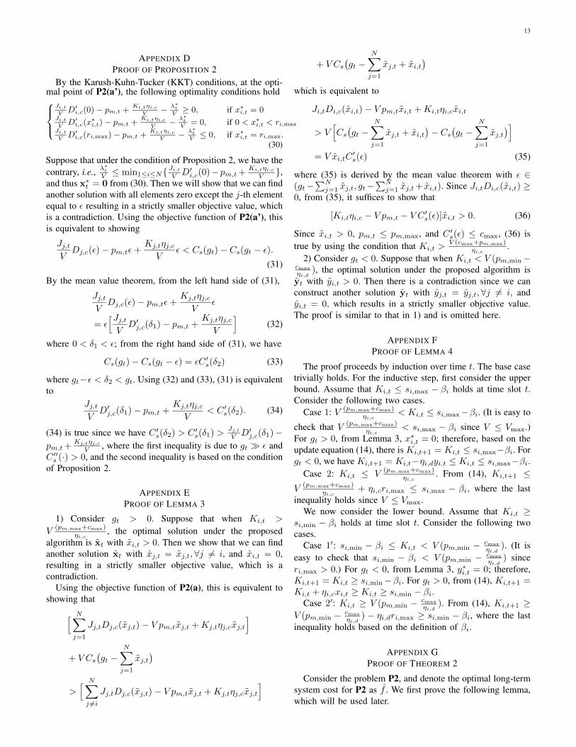
Fig. 1. Schematic representation of a local power grid.

In addition to the limitations summarized above, most ofthese earlier works have omitted to consider some essentialcharacteristics of the aggregator-DS system. For example, adeterministic model is used in [18] and [21], which ignore theuncertainty of the electricity price, and the dynamics of thepower imbalance amount is not incorporated in [25]–[27]. Forthe aggregator, the potential cost for using external energysources to clear the imbalance is ignored in [18]–[22]. ForDS units, the finite battery size constraints are not consideredin [25]; the battery degradation costs due to frequent charg-ing/discharging in real-time operation are omitted in [20]–[22], [25], [26]; the energy gain/loss in charging/dischargingis ignored in [20], [23], [25], [26].

In this work, we consider all above factors missed inprevious works in a more complete aggregator-DS systemmodel. For the system to collectively help a power gridachieve power balance, we develop a real-time distributedalgorithm that does not rely on any statistics of the systemand is easy to implement in reality. Moreover, the proposedalgorithm is proved to be asymptotically optimal as eachDS unit capacity increases. We have previously studied real-time power balancing with an aggregator coordinating staticand dynamic DS units in [23] and [24] respectively, withapplication to frequency regulation using electric vehicles. Themain objective of those works is to fairly allocate the powerimbalance amount among the participants. Furthermore, theaggregator centrally controls the charging and discharging ofthe electric vehicles. In this work, we consider a more realisticcharging and discharging model with battery inefficiency andelectricity prices, beyond others. More importantly, we aim tominimize the long-term system cost and propose a solutionthat can be solved collectively by the aggregator and all DSunits in a distributed manner.

III. SYSTEM MODEL AND PROBLEM STATEMENT

We first describe an aggregator-DS system that providesreal-time power balancing service to a power grid, and thenformulate the problem.

A. Power Balancing and Aggregator-DS System

In a power grid as shown in Fig. 1, due to intrinsic predic-tion error of generation and load as well as the randomnessof renewable sources, the generation amount cannot match the

4

load amount continuously. The discrepancy between these twoat any time can be represented by a power imbalance signal.Consider a time-slotted system with equal time intervals,which in practical systems may range from a few secondsto a few minutes. For ease of notation, we incorporate timeinto the power imbalance signal and use energy units below.At time slot t, we denote gt, |gt| ≤ gmax, as the energyimbalance amount, which is random. If gt > 0, then thegeneration amount is greater than the load amount by gtunits, which results in energy surplus. If gt < 0, then thegeneration amount is less than the load amount by |gt| units,which results in energy deficit. Define 1s,t,1(gt > 0) and1d,t,1(gt < 0) as the indicators of energy surplus andenergy deficit at time slot t, respectively, where 1(·) is theindicator function. Since energy surplus and energy deficitcannot happen simultaneously, we have 1s,t · 1d,t = 0.

Assume that an aggregator serves the power grid and em-ploys energy storage, capable of charging and discharging, toclear the energy imbalance in every time slot. Since the mag-nitude of the energy imbalance signal, |gt|, is in general largeand building a massive energy storage unit could be costly, theaggregator instead coordinates N (smaller) DS units, possiblyowned by different users, to provide power balancing service.These DS units can be, for example, batteries in electricvehicles and batteries deployed at renewable generators. Thenumber of such DS units is expected to be large in thenear future owing to electrification of transportation and theintegration of more and more renewable sources.

At the beginning of time slot t, the aggregator receives theenergy imbalance signal gt from the utility. If gt > 0, theaggregator is required to absorb gt units of energy duringtime slot t. If gt < 0, the aggregator is required to contribute|gt| units of energy during time slot t. Upon receiving theenergy imbalance signal, the aggregator communicates witheach DS unit bidirectionally so as to negotiate the individualenergy absorption or contribution amount. The informationand energy flows of the system are depicted in Fig. 1. Forsimplicity of analysis, in the sequel we assume that all DSunits are static and are connected to the aggregator all the time.Examples of such DS units are batteries deployed at renewablegenerators. The case that involves dynamic DS units, such asbatteries in electric vehicles, will be discussed in Section VIII.

For the i-th DS unit, denote xi,t ≥ 0 as its chargingamount during time slot t in the case of energy surplus, andyi,t ≥ 0 as its discharging amount during time slot t in thecase of energy deficit. Because of limitation imposed by thecharging/discharging circuit, xi,t and yi,t are upper bounded.For simplicity, assume that the maximum allowed chargingand discharging amounts are of the same quantity, denoted byri,max, i.e.,

0 ≤ xi,t ≤ ri,max, 0 ≤ yi,t ≤ ri,max. (1)

Define N -dimensional charging and discharging amountvectors at time slot t as xt,[x1,t, · · · , xN,t] andyt,[y1,t, · · · , yN,t], respectively.

Let ηi,c ∈ (0, 1] be the charging efficiency coefficient of thei-th DS unit, and ηi,d ∈ [1,∞) be the discharging efficiencycoefficient. Because of the battery inefficiency, generally, the

actual stored energy through charging is less than xi,t, and theactual contributed energy through discharging is larger thanyi,t. Denote si,t as the energy state of the i-th DS unit at thebeginning of time slot t. Due to charging and discharging, theenergy state si,t fluctuates over time and evolves as follows1:

si,t+1 = si,t + 1s,tηi,cxi,t − 1d,tηi,dyi,t,si,t + bi,t (2)

where

bi,t,1s,tηi,cxi,t − 1d,tηi,dyi,t (3)

is defined as the effective charging/discharging amount of thei-th DS unit during time slot t.

Charging a battery near its capacity or discharging it closeto the zero energy state can significantly reduce batterylifetime [28]. Therefore, lower and upper bounds on thebattery energy state are usually imposed by its manufactureror owner. Denote si,cap as the energy capacity of the i-th DSunit, and [si,min, si,max] as its preferred energy range with0 ≤ si,min < si,max ≤ si,cap. We assume that the energy stateat each time slot should be limited within the preferred range,i.e.,

si,min ≤ si,t ≤ si,max. (4)

Combining the constraints (1) and (4), we can compactlyrepresent the constraints of xi,t and yi,t as

0 ≤ xi,t ≤ min

{ri,max,

si,max − si,tηi,c

}

and0 ≤ yi,t ≤ min

{ri,max,

si,t − si,min

ηi,d

},

respectively.Since a DS unit absorbs and contributes energy in charging

and discharging, respectively, it has either energy gain orenergy loss when providing real-time power balancing service.Denote the unit market electricity price at time slot t aspm,t ∈ [pm,min, pm,max]. Then, the revenue of the i-th DS unitfor absorbing energy in the case of energy surplus is pm,txi,t,and the loss for contributing energy in the case of energydeficit is pm,tηi,dyi,t. Additionally, by providing power bal-ancing service, each DS unit can receive payment from the ag-gregator for its controllable and flexible charging/dischargingcapability. Denote the unit prices for charging and dischargingservices at time slot t as pc,t and pd,t, respectively. Assumethat the aggregator pays for the charging/discharging based onthe actual service amounts xi,t and yi,t. In other words, thei-th DS unit receives payment pc,txi,t in the case of energysurplus for charging, and payment pd,tyi,t in the case of energydeficit for discharging. As a result, the effective cost of the i-th DS unit for providing power balancing service at time slott is

φi,t,1s,t(−pm,txi,t − pc,txi,t) + 1d,t(pm,tηi,dyi,t − pd,tyi,t).

For each DS unit, offering power balancing service isaccompanied by battery degradation for frequent charging

1We assume that the role of the DS units is to exclusively provide real-timepower balancing service when connected and thus do not explicitly considertheir own charging needs.

5

and extra cycling of battery [29]. Denote Di,c(·) and Di,d(·)as the degradation cost functions with respect to the charg-ing amount and the discharging amount, respectively, withDi,c(0) = Di,d(0) = 0. Since the actual discharging amountis ηi,dyi,t, for notation simplicity, we will merge ηi,d intothe function Di,d(·). Furthermore, since faster charging ordischarging (larger value of xi,t or yi,t) generally has a moredetrimental effect on battery lifetime, Di,c(·) and Di,d(·) canbe approximated by increasing convex functions in general. Tofacilitate later analysis, we slightly strengthen this conditionand take the following assumptions:

C1:• Di,c(·) and Di,d(·) are increasing, strictly convex, and

twice continuously differentiable on [0, ri,max].• The second derivatives of Di,c(·) and Di,d(·) are lower

bounded by a constant di,l > 0 on [0, ri,max].To limit battery degradation, the i-th DS unit sets a pre-designed upper bound li,u ≥ 0 to restrict the long-term degradation cost, which can be formally expressed bylimT→∞

1T

∑T−1t=0 E[1s,tDi,c(xi,t) + 1d,tDi,d(yi,t)] ≤ li,u.

Due to a lack of participating DS units or high batterydegradation cost, sometimes the sum contribution of all DSunits may be insufficient to clear the total power imbalanceamount. Specifically, for energy surplus, this insufficiencymeans that

∑Ni=1 xi,t < gt, and for energy deficit, it means

that∑Ni=1 yi,t < |gt|. Hence, from time to time, to fill the

gap, the aggregator needs to exploit external energy sources,such as the external real-time electricity market2. Denote thecost functions of the external sources for clearing energysurplus and energy deficit as Cs(·) and Cd(·), respectively,with Cs(0) = Cd(0) = 0. Then, the cost of the aggregator forexploiting the external sources at time slot t can be representedas 1s,tCs(gt −

∑Ni=1 xi,t) + 1d,tCd(|gt| −

∑Ni=1 yi,t). We

assume the following conditions on the external cost functions:C2:• Cs(·) and Cd(·) are increasing, strictly convex, and twice

continuously differentiable on [0, gmax].• The second derivatives of Cs(·) and Cd(·) are lower

bounded by a constant cl > 0 on [0, gmax].Finally, the total cost of the aggregator, including that for

using the external sources and the payment to all DS units, isgiven by

ϕt,1s,t

[Cs

(gt −

N∑

i=1

xi,t

)+ pc,t

N∑

i=1

xi,t

]

+ 1d,t

[Cd

(|gt| −

N∑

i=1

yi,t

)+ pd,t

N∑

i=1

yi,t

].

Combining the costs of all DS units with the cost of theaggregator, we have the total cost of the aggregator-DS systemat time slot t given by

wt,(

N∑

i=1

φi,t) + ϕt.

2In practice, the imbalance signal gt may relate to the capacity of theservice provider. In this paper, we focus on the aggregator-DS system, andassume that gt is determined externally and the aggregator guarantees to clearthe imbalance in every time slot.

Notice that the payment for the charging/discharging servicedoes not appear in the expression of wt. This is because suchpayment is transferred from the aggregator to the DS units,hence not affecting the system-wide cost. We will revisit theservice payment in Section V-C.

B. Problem Statement

The aggregator is assumed to be regulated and non profit-driven. For example, it can represent a government-fundedparty that encourages the integration of DS units into a powergrid. The aggregator coordinates the DS units to provide real-time power balancing service, and aims to minimize the long-term system cost while respecting the battery capacity anddegradation cost constraints of each DS unit. We assume thateach DS unit is willing to provide real-time power balancingservice and is under contract with the aggregator. In return,the DS units will be paid for such a service as described inSection III-A3.

We formulate the real-time power balancing problem as thefollowing stochastic optimization problem.

P1: min{xt,yt}

limT→∞

1

T

T−1∑

t=0

E[wt]

s.t. 0 ≤ xi,t ≤ min{ri,max,

si,max − si,tηi,c

},∀i, t (5)

0 ≤ yi,t ≤ min{ri,max,

si,t − si,min

ηi,d

},∀i, t (6)

N∑

i=1

xi,t ≤ 1s,tgt,

N∑

i=1

yi,t ≤ 1d,t|gt|,∀t (7)

limT→∞

1

T

T−1∑

t=0

E[1s,tDi,c(xi,t) + 1d,tDi,d(yi,t)] ≤ li,u,∀i (8)

where the expectations above are taken over the randomsystem state defined as At,(gt, pm,t) and the possibly randomdecisions (xt,yt). The rationale for constraints (5)-(8) isgiven in Section III-A. By (7), we mean that, first, the sumcontribution of all DS units should not exceed the requiredamount, and second, in the case of energy deficit (resp. energysurplus) the charging (resp. discharging) amount of each DSunit should be zero.

The above optimization problem can be solved centrallyby traditional approaches such as dynamic programming [31],provided that the aggregator knows perfectly about the systemstatistics and can fully control the charging/discharging of allDS units. However, for one, dynamic programming is knownto suffer from “the curse of dimensionality,” and accuratestatistics cannot be easily obtained in practice. For another,direct charging/discharging control not only overrides a DSowner’s individual choice but also leads to high computationalcomplexity as the number of participating DS units becomeslarge.

Motivated by these concerns, our goal in this paper isto develop a real-time distributed algorithm, by which the

3We emphasize that the market aspects, such as the contract designinvestigated in [30], are not the focus of this paper.

6

statistics of the system state is not required and each DS unit isable to make its own decision. This is a challenging problemdue to the presence of the dynamic system state, the finitebattery size constraints, and the coupling of decisions amongall DS units. To address this problem, we first decomposethe long-term optimization problem P1 into real-time sub-problems.

IV. DECOMPOSITION INTO REAL-TIME SUB-PROBLEMS

To solve P1, we now propose the corresponding real-time sub-problems under the general framework of Lyapunovoptimization [13], with modifications to handle finite batterysize constraints and to facilitate the distributed algorithmintroduced later.

A. Problem Relaxation

Recall that for each DS unit, the hard constraints of thecharging/discharging amount, i.e., (5) and (6), are equivalentto the constraints (1) and (4). Due to the battery size constraint(4), for each DS unit, the current charging/discharging decisionis coupled with all previous charging/discharging decisionsthrough the current energy state, which complicates the op-timization. To avoid such coupling, we replace (4) with a newtime average constraint and introduce the following relaxedproblem:

P2: min{xt,yt}

limT→∞

1

T

T−1∑

t=0

E[wt]

s.t. (1)(7)(8),

limT→∞

1

T

T−1∑

t=0

E[bi,t] = 0,∀i (9)

where bi,t is defined in (3). As opposed to (4), by which theenergy state is always bounded, (9) requires that the effectivecharging/discharging amount is zero on average.

We now demonstrate that (4) implies (9), so that P2 isindeed a relaxation of P1. Summing both sides of the energystate equation (2) over t ∈ {0, 1, · · · , T − 1} and dividingthem by T yields

si,TT− si,0

T=

1

T

T−1∑

t=0

bi,t. (10)

Taking expectations on both sides of (10) and taking limitsover T gives

limT→∞

E[si,T ]

T− limT→∞

E[si,0]

T= limT→∞

1

T

T−1∑

t=0

E[bi,t]. (11)

Since si,T and si,0 are bounded by (4), the left hand side of(11) is equal to zero and the constraint (9) holds.

By removing the coupling in charging/discharging decisionsdue to the battery size constraints, the relaxed problem P2allows us to apply Lyapunov optimization to decompose theoriginal problem into real-time sub-problems. We will showlater in Section VI that our developed solution in fact alsosatisfies (4), so it is feasible for P1. This relaxation technique

to accommodate the type of time-coupled decision constraintssuch as (5) and (6) was first introduced in [32] for energymanagement in a data center equipped with an ideal battery,and later was also applied in [16] and [17]. Compared with[32], besides our problem being different from it, we considermultiple DS units. Compared with [16] and [17], the struc-ture of our problem is more complicated, with a nonlinearobjective which allows for bidirectional energy flow betweenthe aggregator and DS units. Thus, it is more involved in therelaxation treatment to ensure that the battery size constraintsare satisfied.

B. Virtual Queue Design

To solve P2, we introduce virtual queues and transformthe time average constraints (8) and (9) to queue stabilityconstraints, as explained below.

Consider constraint (8). To facilitate distributed implemen-tation which will be explained later, we add a constant costcushion ai > 0 to both sides of (8), and obtain the followingequivalent constraint for each DS unit:

limT→∞

1

T

T−1∑

t=0

E[1s,tDi,c(xi,t) + 1d,tDi,d(yi,t) + ai] ≤ li,u

(12)

where li,u,li,u+ai. Define a virtual queue Ji,t, which updatesas

Ji,t+1 = max{Ji,t − li,u, 0}+ 1s,tDi,c(xi,t)

+ 1d,tDi,d(yi,t) + ai. (13)

Initialize Ji,0 = ai and define Jt,[J1,t, · · · , JN,t]. Basedon (13), queue backlog Ji,t accumulates the total amount ofdegradation cost in excess of li,u. The function of ai is toguarantee that Ji,t ≥ ai. The introduction of ai is important,and we will discuss the design of ai in Section V-B.

For constraint (9), we associate it with a virtual queue Ki,t,which evolves as

Ki,t+1 = Ki,t + bi,t. (14)

Define Kt,[K1,t, · · · ,KN,t]. By (14), Ki,t accumulates thetotal effective charging/discharging amount. Comparing (14)with (2), we can see that Ki,t and the energy state si,t evolvein the same manner. We relate them by initializing Ki,0 =si,0 − βi, where the shift parameter βi is set to be

βi,si,min + ηi,dri,max − V(pm,min −

cmax

ηi,d

), (15)

where cmax,max{C ′s(gmax), C ′d(gmax)} and the weight V ∈(0, Vmax] with

Vmax, min1≤i≤N

{si,max − si,min − (ηi,c + ηi,d)ri,max

cmax+pm,max

ηi,c+ cmax

ηi,d− pm,min

}.

(16)

Thus, the virtual queue Ki,t is a shifted version of the energystate si,t. Ki,t is introduced to track si,t. More importantly, aswe will see later, the boundedness of si,t can be guaranteed

7

through the control of Ki,t. The design of βi and Vmax in(15) and (16) is crucial. We will show in Section VI-B howthe constraint (4) can be guaranteed by such design.

Note that under the real-time operation, the value of ri,max

in (16) is generally much smaller than the energy capacity.For example, for the 2012 Ford Focus Electric, the energycapacity is 23 kWh and the maximum charging/dischargingrate is 6.6 kW. Assuming that the duration of each time slotis 5 minutes, we then have ri,max = 0.55 kWh � 23 kWh.By this observation, from (16), we have Vmax > 0 in general.

Finally, we show that the time-averaged constraints (8) and(9) can be transformed into the mean rate stability constraintsof virtual queues, which is a direct result from [13].

Lemma 1: Constraints (8) and (9) hold if the virtual queuesJi,t and Ki,t are mean rate stable, respectively.

C. Real-Time Sub-Problems

At time slot t, define a vector Θt,[Jt,Kt], the Lyapunovfunction L(Θt), 1

2

∑Ni=1(J2

i,t+K2i,t), and the associated one-

slot Lyapunov drift

∆(Θt),E [L(Θt+1)− L(Θt)|Θt] .

The drift-plus-cost function is defined as ∆(Θt)+V E[wt|Θt][13], in which the time-averaged constraints and the objectivefunction are jointly considered, with the weight V (the sameV as in (15)) controlling their trade-off. In the followingproposition, we provide an upper bound on the drift-plus-costfunction.

Proposition 1: For all possible policies of the charg-ing/discharging decisions of all DS units, and all possiblevalues of Θt, the drift-plus-cost function is upper boundedas follows:

∆(Θt) + V E[wt|Θt] ≤ B + V E[wt|Θt] +

N∑

i=1

Ki,tE[bi,t|Θt]

+

N∑

i=1

Ji,tE[1s,tDi,c(xi,t) + 1d,tDi,d(yi,t)− li,u|Θt] (17)

where

B,1

2

N∑

i=1

[l2i,u +(

max{Di,c(ri,max), Di,d(ri,max)}+ ai)2

+ r2i,max], (18)

and V ∈ (0, Vmax].Proof: See Appendix A.

Adopting the general framework of Lyapunov optimization[13], we design a real-time algorithm to minimize the upperbound of the drift-plus-cost function on the right hand side of(17). The algorithm can lead to a guaranteed performance asshown in Section VI. Consequently, we consider the real-timesub-problems for energy surplus and energy deficit at eachtime slot t as follows. For notation simplicity, we will omitthe subscript t of the optimization variables whenever it isclear from the context.

P2(a) (energy surplus):

minx

[N∑

i=1

Ji,tDi,c(xi)− V pm,txi +Ki,tηi,cxi

]

+ V Cs

(gt −

N∑

i=1

xi

)

s.t. 0 ≤ xi ≤ ri,max,

N∑

i=1

xi ≤ gt.

P2(b) (energy deficit):

miny

[N∑

i=1

Ji,tDi,d(yi) + V pm,tηi,dyi −Ki,tηi,dyi

]

+ V Cd

(|gt| −

N∑

i=1

yi

)

s.t. 0 ≤ yi ≤ ri,max,N∑

i=1

yi ≤ |gt|.

The optimization variables x and y are N -dimensional vectorswith the i-th element being xi and yi, respectively.

V. DISTRIBUTED ALGORITHM FOR REAL-TIMESUB-PROBLEMS

The real-time sub-problems P2(a) and P2(b) can be solvedby the aggregator in a centralized way. However, since theDS units may belong to different users, they may not bewilling to relinquish direct control of charging/discharging tothe aggregator. In addition, the computational complexity ofcentralized control would grow too quickly as the numberof DS units increases. In this section, we employ Lagrangedual decomposition and adapt a fast iterative algorithm tosolve P2(a) and P2(b) distributively. Since energy surplus andenergy deficit cannot happen simultaneously and their analysesare similar, in the following, we focus on the energy surplusproblem P2(a).

A. Lagrange Dual Decomposition

In P2(a), since Ji,t ≥ ai > 0 and Di,c(·) is strictly convex,the objective function is strictly convex, which means thatthere is at most one global minimizer. Additionally, since theobjective function is continuous and the constraint set of x iscompact, there is at least one minimizer. Therefore, P2(a) hasa unique solution.

However, we note that the term Cs(gt −∑Ni=1 xi) in the

objective function and the term∑Ni=1 xi ≤ gt in the constraint

are functions of the charging amounts of all DS units, whichhinders a distributed algorithm. To avoid such coupling, wefirst introduce an auxiliary variable q ∈ [0, gt] to represent thedifference between the energy imbalance amount and the sumcontribution of all DS units, i.e., gt −

∑Ni=1 xi, and consider

the following problem.P2(a’):

minx,q

[N∑

i=1

Ji,tDi,c(xi)− V pm,txi +Ki,tηi,cxi

]+ V Cs(q)

8

s.t. 0 ≤ xi ≤ ri,max, 0 ≤ q ≤ gt, (19)N∑

i=1

xi + q = gt. (20)

It is clearly that P2(a’) and P2(a) are equivalent and have thesame unique solution in x.

Next we associate the equality constraint (20) with a La-grange multiplier λ. The partial Lagrangian of P2(a’) is

Ft(x, q, λ) =

[N∑

i=1

Ji,tDi,c(xi)− V pm,txi +Ki,tηi,cxi

]

+ V Cs(q) + λ

(gt −

N∑

i=1

xi − q

).

The dual function Gt(λ) is defined as the partial minimum ofFt(x, q, λ) with respect to the primal variables x and q:

Gt(λ) = minx,q

Ft(x, q, λ) s.t. (19).

Note that Gt(λ) can be naturally decomposed into sub-problems for each DS unit and the aggregator. Specifically,with Gt(λ) divided by V , the sub-problem for each DS unitis

minxi

−pm,txi −λ

Vxi +

Ji,tVDi,c(xi) +

Ki,tηi,cV

xi (21)

s.t. 0 ≤ xi ≤ ri,max,

while the sub-problem for the aggregator is

minq

Cs(q) +λ

V(gt − q) s.t. 0 ≤ q ≤ gt. (22)

In (21), by interpreting λV as pc,t, the unit price for charging

service as defined in Section III-A, we can view the objectiveof the i-th DS unit as minimizing the weighted sum of itsdifferent costs. By the Karush-Kuhn-Tucker (KKT) conditions,given λ, we obtain the unique solution of (21) in closedform: [(D′i,c)

−1(V pm,t+λ−Ki,tηi,c

Ji,t

)]ri,max

0 . In the optimizationproblem (22), the aggregator minimizes its cost, includingthe external energy cost and the payment to all DS units.Again, the unique solution of (22) is found in closed form:[(C ′s)

−1( λV )]gt0 . Thus, for any given λ, there is a unique so-lution for both (21) and (22). Consequently, the dual functionGt(λ) is continuously differentiable in R [33].

The Lagrange dual problem is defined as the maximizationof the dual function:

maxλ

Gt(λ). (23)

Denote the optimal solution of the dual problem at time slot tas λ∗t , and the unique optimal solution of P2(a’) at time slott as (x∗t , q

∗t ). Verifying Slater’s condition on P2(a’), we are

assured to have strong duality between the primal P2(a’) andits dual (23) [14]. Thus, at time slot t, using λ∗t , we can recoverthe optimal solution (x∗t , q

∗t ) by solving the sub-problems (21)

and (22) [33].To solve (23), we propose a fast iterative algorithm pre-

sented in the next subsection.

Algorithm 1: Distributed algorithm to solve the dual ofP2(a’).

begin Aggregator’s algorithm:Initialize: k = 1; γ1 = λ0 ∈ R; ν1 = 1; µ, ε > 0.repeat

Broadcast γk; receive xki ,∀i.qk ← [(C ′s)

−1(γk

V )]gt0 ;λk ← γk + µ

(gt −

∑Ni=1 x

ki − qk

);

νk+1 ← 1+√

1+4(νk)2

2 ;γk+1 ← λk + νk−1

νk+1 (λk − λk−1);k ← k + 1.

until |gt −∑Ni=1 x

ki − qk| < ε;

Output: q∗t = qk.begin DS’s algorithm:

repeatReceive γk;xki ← [(D′i,c)

−1(V pm,t+γk−Ki,tηi,c

Ji,t

)]ri,max

0 ;send xki .

until;Output: x∗i,t = xki .

B. Dual Maximization with FISTA and Convergence Analysis

Since we consider the real-time power balancing problemwith a short time interval, it is highly desirable that thealgorithm can converge quickly in each time slot. To thisend, we adapt a fast iterative shrinkage-thresholding algorithm(FISTA) [15] to solve the dual problem (23). The proposedalgorithm is summarized in Algorithm 1. Compared with thestandard gradient algorithm in which the Lagrange multiplierλk is updated from the previous iterate λk−1, in Algorithm1, λk is updated from γk, which is designed as a linearcombination of the previous two iterates λk−1 and λk−2.Nonetheless, the extra computation is marginal.

Below we show that the gradient of the dual function isLipschitz continuous, and determine its Lipschitz constant.The result is crucial for the convergence analysis of Algorithm1.

Lemma 2: Under the conditions C1 and C2, the gradientof the dual function is Lipschitz continuous, i.e., we have|G′t(λ1) − G′t(λ2)| ≤ ρ|λ1 − λ2| for all λ1, λ2 ∈ R, wherethe Lipschitz constant ρ is given by

ρ,(N + 1) max

{1

a1d1,l, · · · , 1

aNdN,l,

1

V cl

}, (24)

where di,l and cl are given in C1 and C2, respectively, and aiis the cost cushion parameter in (12).

Proof: See Appendix B.In (24), since ai > 0, we have 0 < ρ < ∞. Using Lemma

2, we now prove the convergence of Algorithm 1.Theorem 1: Under the conditions C1 and C2, in Algorithm

1, with step size µ ∈ (0, µ0] where µ0,1/ρ, the sequence{λk} converges to the optimum λ∗t of the dual problem (23).Furthermore, for any k ≥ 1,

Gt(λ∗t )−Gt(λk) ≤ 2|λ0 − λ∗t |2

µ(k + 1)2,

9

where λ0 is the initial value of λ.Proof: Given Lemma 2, the proof is similar to that in

[15] with minor modification. See Appendix C.Theorem 1 suggests that Algorithm 1 has a worst-case

convergence rate of O(1/k2). In comparison, the standardgradient algorithm, which is used in [17]4 among many others,has a worst-case convergence rate O(1/k). Also from Theorem1, the step size µ is upper bounded by µ0, the inverse ofthe Lipschitz constant ρ. Based on the definition of ρ, weroughly have that, the larger the number of DS units, thesmaller µ0 hence the slower the algorithm, which conformsto our intuition.

Furthermore, from (24), µ0 is a strictly increasing functionof the cost cushion ai in the interval (0, V cldi,l

]. Therefore, forthe sole purpose of faster convergence, a larger ai should bechosen. However, later in Section VI-C, we will show thatusing a smaller ai may decrease the system cost.

C. Price Signaling pc,tWe now look at the property of the optimal charging price

signal p∗c,t =λ∗tV . Since DS units have energy gain by charging,

λ∗tV can be negative. Below, we give a condition under whichλ∗tV is lower bounded and there exists a DS unit willing toprovide power balancing service.

Proposition 2: At time slot t, if there exists a DS unit jsuch that −pm,t+ Jj,t

V D′j,c(x)+Kj,tηj,c

V < C ′s(x),∀x ∈ (0, ε),where ε is an arbitrarily small positive number, then the pricesignal λ∗t

V is lower bounded as

λ∗tV

> min1≤i≤N

{−pm,t +

Ji,tVD′i,c(0) +

Ki,tηi,cV

}

and the charging amount x∗j,t > 0.Proof: See Appendix D.

Proposition 2 essentially states that, as long as there is aDS unit whose effective marginal cost, considering both theenergy gain and the charging/discharging cost, is strictly lessthan the marginal cost of the external energy source, it isbeneficial for the aggregator to incentivize the DS units toprovide power balancing service (even though the price signalcan be negative).

VI. MAIN ALGORITHM AND PERFORMANCE OPTIMALITY

In this section, we give the main algorithm that combinesthe components presented in Sections IV and V, and analyzeits performance with respect to our original problem P1.

A. Main Algorithm

In Algorithm 2, we formally state the real-time distributedalgorithm for the aggregator-DS system to provide powerbalancing service. For presentation simplicity, we focus onthe energy surplus case only.

We now discuss the information required in Algorithm 2and show that Algorithm 2 can be easily implemented in

4The subgradient algorithm used in [17] reduces to the gradient algorithmwhen the dual function is differentiable.

Algorithm 2: Main algorithm: real-time distributed algo-rithm for power balancing.

begin Aggregator’s algorithm:Repeat at each time:

1) Observe gt.2) Broadcast 1s,t.3) Execute aggregator’s algorithm in Algorithm 1.

begin DS’s algorithm:Initialize: Ji,0 = ai; Ki,0 = si,0 − βi.Repeat at each time:

1) Observe pm,t, 1s,t, Ji,t, and Ki,t.2) Execute DS’s algorithm in Algorithm 1.3) Update Ji,t and Ki,t based on (13) and (14),

respectively.

practice. In Algorithm 2, the statistical information of thesystem is not required, and only instantaneous observationsare needed, which can be obtained either locally or throughsimple communication. Specifically, at each time slot t, theaggregator observes the energy imbalance signal gt, and eachDS unit observes the electricity price pm,t, the indicator ofthe energy imbalance signal 1s,t, and the queue backlogs Ji,tand Ki,t. To initialize Ji,0 and Ki,0 at each DS unit, theaggregator broadcasts V , cl, and cmax to all DS units at theinitial time. For the aggregator to determine Vmax in (16), thevalues of ηi,c, ηi,d, and si,max − si,min − (ηi,c + ηi,d)ri,max

at each DS unit are required. In practice, however, it may beunnecessary to acquire all such information for determiningVmax. Note that as argued in Section IV-B the maximumallowed charging/discharging amount ri,max is much smallercompared with the energy capacity. Thus, when the batteryhas high charging/discharging efficiency, i.e., ηi,c and ηi,d areclose to 1, approximately only the minimum battery capacityamong all DS units is required for the design of Vmax.

B. Boundedness of Energy State

The proposed algorithm in Algorithm 2 is designed for P2,in which the battery size constraint (4) in P1 is replaced bythe relaxed time average constraint (9). Thus, with {x∗t ,y∗t }, itis not yet certain whether the resultant si,t violates the batterysize constraint (4), thus becoming infeasible for P1. We nowdemonstrate that under the proposed algorithm, si,t in factalways satisfies (4).

Since the virtual queue Ki,t is designed to be a shiftedversion of si,t, to prove the boundedness of si,t, it suffices toshow that Ki,t is restricted within a shifted preferred range. Wefirst show through the following lemma that, Ki,t is boundedfor any initial value Ki,0.

Lemma 3: For any initial value Ki,0,1) if gt > 0 and Ki,t > V

(pm,max+cmax)ηi,c

, x∗i,t = 0;2) if gt < 0 and Ki,t < V (pm,min − cmax

ηi,d), y∗i,t = 0.

Proof: See Appendix E.Lemma 3 says that, given any Ki,0, for energy surplus, if

Ki,t is greater than the above threshold, the resultant chargingamount is zero, and thus Ki,t+1 cannot be increased at thenext time slot. Similarly, for energy deficit, if Ki,t is less than

10

the above threshold, the resultant discharging amount is zero,and thus Ki,t+1 cannot be decreased at the next time slot.Therefore, Ki,t is bounded.

Using Lemma 3, we next show that by our designedinitialization, Ki,t is bounded within a shifted preferred range.

Lemma 4: Given Ki,0 = si,0 − βi, where βi is definedin (15), the queue backlog Ki,t is bounded within [si,min −βi, si,max − βi] for all time slot t.

Proof: See Appendix F.Remarks on Choices of βi and Vmax: To track the energy

state si,t, in principle, the shift βi could be any value.However, as required in Case 2′ of the proof of Lemma 4,βi should be lower bounded, i.e., βi = si,min + ηi,dri,max −V (pm,min − cmax

ηi,d) + ε1 for any ε1 ≥ 0. Furthermore, as

required in Case 1 of the proof, it is sufficient to set Vmax =

min1≤i≤N

{si,max−si,min−ηi,dri,max−ε1−ε2cmax+pm,max

ηi,c+ cmaxηi,d−pm,min

}with any ε2 > 0.

Finally, to facilitate Case 2 of the proof, we set ε1 and ε2to be 0 and ηi,cri,max, respectively, to make Vmax as large aspossible. (As shown in Theorems 2 and 3 below, a larger Vmax

implies better performance by the proposed algorithm.) Thisleads to the specific designs as shown in (15) and (16).

By Lemma 4, the boundedness of the energy state si,t isstraightforward, and is given in the following lemma.

Lemma 5: Under the proposed algorithm, the energy statesi,t is bounded within [si,min, si,max] for all time slot t.

C. Optimality Analysis

Denote the long-term system cost under the proposed algo-rithm as f∗ and that under the optimal solution for P1 asf opt. Note that the optimal solution may require statisticalinformation of the system. The optimality of the proposedalgorithm is described in Theorems 2 and 3.

Theorem 2: Suppose that the system state At is i.i.d. overtime.

1) The virtual queues Ji,t and Ki,t are mean rate stable, and{x∗t ,y∗t } is feasible for P1;

2) f∗ ≤ f opt + BV , where B is defined in (18) and V ∈

(0, Vmax].Proof: See Appendix G.

From Theorem 2, the system cost under the proposedalgorithm is away from the optimum by O(1/V ). Thus, thelarger V , the better the performance of the proposed algorithm.However, in practice, due to the boundedness of the preferredenergy range, V cannot be arbitrarily large and is upperbounded by Vmax, whose design rationale is given in theremarks after Lemma 4.

Based on the definition of Vmax in (16), Vmax increaseswith the smallest span of the DS units’ preferred ranges,i.e., min1≤i≤N{si,max−si,min}. Therefore, roughly speaking,the performance gap between the proposed algorithm and theoptimum decreases as the smallest battery capacity increases.Asymptotically, as each DS unit’s battery capacity goes toinfinity, the proposed algorithm achieves the optimum.

We also note that the cost cushion ai increases the per-formance bound through the constant B. Hence, a smaller aiis desirable. Combining this with the convergence analysis in

Section V-B, we observe the important role of ai as a tuningparameter in the trade-off between system performance andconvergence speed.

In Theorem 2, the i.i.d. condition of At can be relaxed toMarkovian, and a similar performance bound can be obtained.This allows us to design aggregator-DS systems in the casewhen the power imbalance amount gt and the electricity pricepm,t are Markovian over time.

Theorem 3: Suppose that the system state At evolves basedon a finite state irreducible and aperiodic Markov chain.

1) The virtual queues Ji,t and Ki,t are mean rate stable, and{x∗t ,y∗t } is feasible for P1;

2) f∗ ≤ f opt +O(1/V ), where V ∈ (0, Vmax].

Proof: The above results can be proved by expanding theproof of Theorem 2 using a multi-slot drift technique [13]. Weomit the proof here for brevity.

VII. NUMERICAL ANALYSIS

In the previous section, we have proven the analyticalperformance bound and asymptotic optimality of the proposedalgorithm. In this section, we present numerical evaluation ofthe algorithm. Since as explained in Section II, the previousworks on power balancing with the distributed aggregator-DSsystem, e.g., [25]–[27], study system models that are differentand simpler than ours, they are not applicable for numericalcomparison. Instead, we consider a greedy algorithm as abenchmark.

A. Simulation Setup

We have developed an aggregator-DS model in Matlab.Unless otherwise specified, the following parameters are set asdefault. The aggregator is connected with N = 150 DS units,each with energy capacity si,cap = 23 kWh and maximumcharging/discharging rate 6.6 kW (based on the 2012 FordFocus Electric). The duration of each time slot is ∆t = 30seconds. Then, the maximum allowed charging/dischargingamount of each DS unit is ri,max = 6.6∆t

3600 kWh. Thecharging and discharging efficiency coefficients are ηi,c = 0.8and ηi,d = 1.2, respectively. The preferred energy range ofeach DS unit is [0.1si,cap, 0.9si,cap], from which the initialenergy state si,0 is uniformly drawn. The degradation costfunctions of the charging/discharging amount are Di,c(x) =

Di,d(x) = x1.5, and the upper bound li,u =( ri,max

2

)1.5. The

energy imbalance signal gt is i.i.d. over time and is sampleduniformly from [−gmax, gmax], where gmax =

∑Ni=1 ri,max.

The unit market electricity price is 7 cents/kWh, which isthe current off-peak electricity price in Ontario [34]. Theexternal cost functions for clearing energy surplus and energydeficit are Cs(x) = Cd(x) = 7x1.2. To determine thecharging/discharging amounts of DS units at each time slott, we apply the proposed algorithm in Algorithm 2 withV = Vmax. The cost cushion parameter ai = Vmaxcl

di,lby default

for fast convergence.

11

TABLE IINUMBER OF ITERATIONS FOR |gt −

∑Ni=1 x

ki − qk| < 0.01.

µ/µ0 1 10 20 50 100

ai = Vmaxcl/di,l 279 105 85 45 26

ai = Vmaxcl/(4di,l) 964 411 183 131 44

B. Convergence of Distributed AlgorithmIn Table II, we show the convergence speed of Algo-

rithm 1 by listing the number of iterations required for|gt−

∑Ni=1 x

ki−qk| < 0.01, when the current energy imbalance

signal gt = gmax. From Table II, when the step size µ = µ0,with the default ai, the algorithm converges within 279 steps;in contrast, when ai is a quarter of the default value, thealgorithm takes 964 steps to converge as the applied µ0 nowis much smaller. We also observe that the convergence speedcan be significantly improved by increasing µ, indicating therobustness of the algorithm to the step size design.

C. Comparison with Greedy AlgorithmAs a benchmark, we consider a greedy algorithm that

is applied to the same system model as ours but aims toindependently minimize the system cost at each time slot.Specifically, the charging/discharging amounts of the DS unitsunder the greedy algorithm is determined by the followingoptimization problem at each time slot t.

minxt,yt

wt

s.t. (5)(6)(7),1s,tDi,c(xi,t) + 1d,tDi,d(yi,t) ≤ li,u,∀i.

The above problem produces a feasible solution for P1 at eachtime t and can be implemented distributively following thetechnique in Section V.

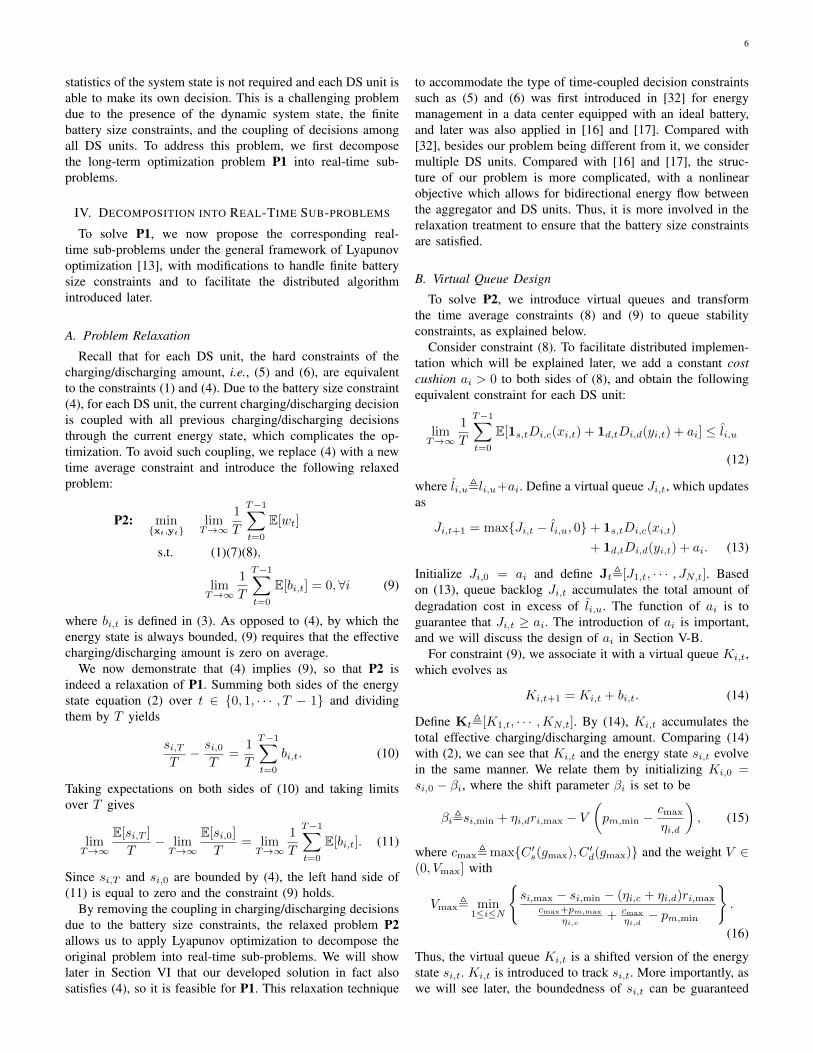
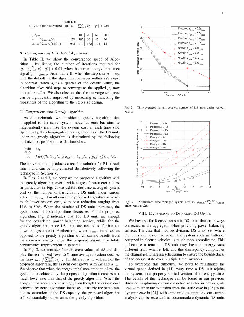
In Figs. 2 and 3, we compare the proposed algorithm withthe greedy algorithm over a wide range of parameter values.In particular, in Fig. 2, we exhibit the time-averaged systemcost vs. the number of participating DS units under variousvalues of si,max. For all cases, the proposed algorithm achievesmuch lower system cost, with cost reduction ranging from11% to 80%. When the number of DS units increases, thesystem cost of both algorithms decreases. For the proposedalgorithm, Fig. 2 indicates that 150 DS units are enoughfor the considered power balancing service, while for thegreedy algorithm, more DS units are needed to further cutdown the system cost. Furthermore, when si,max increases, asopposed to the greedy algorithm which cannot benefit fromthe increased energy range, the proposed algorithm exhibitsperformance improvement in general.

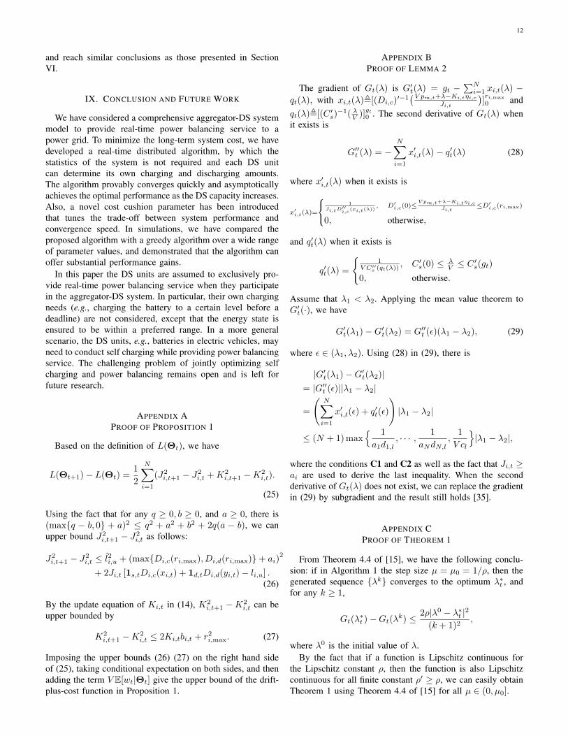
In Fig. 3, we consider four different values of ∆t and dis-play the normalized (over ∆t) time-averaged system cost vs.the ratio gmax/

∑150i=1 ri,max for different gmax values. For the

proposed algorithm, the system cost grows with ∆t and gmax.We observe that when the energy imbalance amount is low, thesystem cost achieved by the proposed algorithm increases at amuch lower rate than that of the greedy algorithm. When theenergy imbalance amount is high, even though the system costachieved by both algorithms increases at nearly the same ratedue to saturation of the DS capacity, the proposed algorithmstill substantially outperforms the greedy algorithm.

50 100 150 2000

5

10

15

20

25

30

Number of DS units

Tim

e−

avera

ged s

yste

m c

ost

Proposed: s

i,max = 0.3s

i,cap

Proposed: si,max

= 0.5si,cap

Proposed: si,max

= 0.7si,cap

Proposed: si,max

= 0.9si,cap

Greedy: si,max

= 0.3si,cap

Greedy: si,max

= 0.5si,cap

Greedy: si,max

= 0.7si,cap

Greedy: si,max

= 0.9si,cap

Fig. 2. Time-averaged system cost vs. number of DS units under varioussi,max.

0.8 0.9 1 1.1 1.2 1.3 1.4 1.5 1.60

0.2

0.4

0.6

0.8

1

1.2

1.4

gmax/∑150

i=1ri,max

Norm

alized tim

e−

avera

ged s

yste

m c

ost

Proposed: ∆t = 5s

Proposed: ∆t = 10s

Proposed: ∆t = 30s

Proposed: ∆t = 60s

Greedy: ∆t = 5s

Greedy: ∆t = 10s

Greedy: ∆t = 30s

Greedy: ∆t = 60s

Fig. 3. Normalized time-averaged system cost vs. gmax/∑150i=1 ri,max

under various ∆t.

VIII. EXTENSION TO DYNAMIC DS UNITS

We have so far focused on static DS units that are alwaysconnected to the aggregator when providing power balancingservice. The case that involves dynamic DS units, i.e., whereDS units can leave and rejoin the system such as batteriesequipped in electric vehicles, is much more complicated. Thisis because a returning DS unit may have an energy statedifferent from when it left, and this discrepancy complicatesthe charging/discharging scheduling to ensure the boundednessof the energy state over multiple time instances.

To overcome this difficulty, we need to reinitialize thevirtual queue defined in (14) every time a DS unit rejoinsthe system, to a properly shifted version of its energy state.The details of this technique can be found in our previousstudy on employing dynamic electric vehicles in power grids[24]. Similar to the extension from the static case in [23] to thedynamic case in [24], with some mild assumptions, our currentanalysis can be extended to accommodate dynamic DS units

12

and reach similar conclusions as those presented in SectionVI.

IX. CONCLUSION AND FUTURE WORK

We have considered a comprehensive aggregator-DS systemmodel to provide real-time power balancing service to apower grid. To minimize the long-term system cost, we havedeveloped a real-time distributed algorithm, by which thestatistics of the system is not required and each DS unitcan determine its own charging and discharging amounts.The algorithm provably converges quickly and asymptoticallyachieves the optimal performance as the DS capacity increases.Also, a novel cost cushion parameter has been introducedthat tunes the trade-off between system performance andconvergence speed. In simulations, we have compared theproposed algorithm with a greedy algorithm over a wide rangeof parameter values, and demonstrated that the algorithm canoffer substantial performance gains.

In this paper the DS units are assumed to exclusively pro-vide real-time power balancing service when they participatein the aggregator-DS system. In particular, their own chargingneeds (e.g., charging the battery to a certain level before adeadline) are not considered, except that the energy state isensured to be within a preferred range. In a more generalscenario, the DS units, e.g., batteries in electric vehicles, mayneed to conduct self charging while providing power balancingservice. The challenging problem of jointly optimizing selfcharging and power balancing remains open and is left forfuture research.

APPENDIX APROOF OF PROPOSITION 1

Based on the definition of L(Θt), we have

L(Θt+1)− L(Θt) =1

2

N∑

i=1

(J2i,t+1 − J2

i,t +K2i,t+1 −K2

i,t).

(25)

Using the fact that for any q ≥ 0, b ≥ 0, and a ≥ 0, there is(max{q − b, 0} + a)2 ≤ q2 + a2 + b2 + 2q(a − b), we canupper bound J2

i,t+1 − J2i,t as follows:

J2i,t+1 − J2

i,t ≤ l2i,u + (max{Di,c(ri,max), Di,d(ri,max)}+ ai)2

+ 2Ji,t [1s,tDi,c(xi,t) + 1d,tDi,d(yi,t)− li,u] .(26)

By the update equation of Ki,t in (14), K2i,t+1 −K2

i,t can beupper bounded by

K2i,t+1 −K2

i,t ≤ 2Ki,tbi,t + r2i,max. (27)

Imposing the upper bounds (26) (27) on the right hand sideof (25), taking conditional expectation on both sides, and thenadding the term V E[wt|Θt] give the upper bound of the drift-plus-cost function in Proposition 1.

APPENDIX BPROOF OF LEMMA 2

The gradient of Gt(λ) is G′t(λ) = gt −∑Ni=1 xi,t(λ) −

qt(λ), with xi,t(λ),[(Di,c)′−1(V pm,t+λ−Ki,tηi,c

Ji,t

)]ri,max

0 andqt(λ),[(C ′s)

−1( λV )]gt0 . The second derivative of Gt(λ) whenit exists is

G′′t (λ) = −N∑

i=1

x′i,t(λ)− q′t(λ) (28)

where x′i,t(λ) when it exists is

x′i,t(λ)=

1

Ji,tD′′i,c

(xi,t(λ)), D′i,c(0)≤

V pm,t+λ−Ki,tηi,cJi,t

≤D′i,c(ri,max)

0, otherwise,

and q′t(λ) when it exists is

q′t(λ) =

{1

V C′′s (qt(λ)) , C ′s(0) ≤ λV ≤ C

′s(gt)

0, otherwise.

Assume that λ1 < λ2. Applying the mean value theorem toG′t(·), we have

G′t(λ1)−G′t(λ2) = G′′t (ε)(λ1 − λ2), (29)

where ε ∈ (λ1, λ2). Using (28) in (29), there is

|G′t(λ1)−G′t(λ2)|= |G′′t (ε)||λ1 − λ2|

=

(N∑

i=1

x′i,t(ε) + q′t(ε)

)|λ1 − λ2|

≤ (N + 1) max{ 1

a1d1,l, · · · , 1

aNdN,l,

1

V cl

}|λ1 − λ2|,

where the conditions C1 and C2 as well as the fact that Ji,t ≥ai are used to derive the last inequality. When the secondderivative of Gt(λ) does not exist, we can replace the gradientin (29) by subgradient and the result still holds [35].

APPENDIX CPROOF OF THEOREM 1

From Theorem 4.4 of [15], we have the following conclu-sion: if in Algorithm 1 the step size µ = µ0 = 1/ρ, then thegenerated sequence {λk} converges to the optimum λ∗t , andfor any k ≥ 1,

Gt(λ∗t )−Gt(λk) ≤ 2ρ|λ0 − λ∗t |2

(k + 1)2,

where λ0 is the initial value of λ.By the fact that if a function is Lipschitz continuous for

the Lipschitz constant ρ, then the function is also Lipschitzcontinuous for all finite constant ρ′ ≥ ρ, we can easily obtainTheorem 1 using Theorem 4.4 of [15] for all µ ∈ (0, µ0].

13

APPENDIX DPROOF OF PROPOSITION 2

By the Karush-Kuhn-Tucker (KKT) conditions, at the opti-mal point of P2(a’), the following optimality conditions holdJi,tV

D′i,c(0)− pm,t +Ki,tηi,c

V− λ∗t

V≥ 0, if x∗i,t = 0

Ji,tV

D′i,c(x∗i,t)− pm,t +

Ki,tηi,cV

− λ∗tV

= 0, if 0 < x∗i,t < ri,maxJi,tV

D′i,c(ri,max)− pm,t +Ki,tηi,c

V− λ∗t

V≤ 0, if x∗i,t = ri,max.

(30)

Suppose that under the condition of Proposition 2, we have thecontrary, i.e., λ

∗t

V ≤ min1≤i≤N{Ji,tV D′i,c(0)− pm,t+Ki,tηi,c

V },and thus x∗t = 0 from (30). Then we will show that we can findanother solution with all elements zero except the j-th elementequal to ε resulting in a strictly smaller objective value, whichis a contradiction. Using the objective function of P2(a’), thisis equivalent to showing

Jj,tVDj,c(ε)− pm,tε+

Kj,tηj,cV

ε < Cs(gt)− Cs(gt − ε).(31)

By the mean value theorem, from the left hand side of (31),

Jj,tVDj,c(ε)− pm,tε+

Kj,tηj,cV

ε

= ε[Jj,tVD′j,c(δ1)− pm,t +

Kj,tηj,cV

](32)

where 0 < δ1 < ε; from the right hand side of (31), we have

Cs(gt)− Cs(gt − ε) = εC ′s(δ2) (33)

where gt−ε < δ2 < gt. Using (32) and (33), (31) is equivalentto

Jj,tVD′j,c(δ1)− pm,t +

Kj,tηj,cV

< C ′s(δ2). (34)

(34) is true since we have C ′s(δ2) > C ′s(δ1) >Jj,tV D′j,c(δ1)−

pm,t+Kj,tηj,c

V , where the first inequality is due to gt � ε andC ′′s (·) > 0, and the second inequality is based on the conditionof Proposition 2.

APPENDIX EPROOF OF LEMMA 3

1) Consider gt > 0. Suppose that when Ki,t >

V(pm,max+cmax)

ηi,c, the optimal solution under the proposed

algorithm is xt with xi,t > 0. Then we show that we can findanother solution xt with xj,t = xj,t,∀j 6= i, and xi,t = 0,resulting in a strictly smaller objective value, which is acontradiction.

Using the objective function of P2(a), this is equivalent toshowing that

[ N∑

j=1

Jj,tDj,c(xj,t)− V pm,txj,t +Kj,tηj,cxj,t

]

+ V Cs(gt −

N∑

j=1

xj,t)

>[ N∑

j 6=i

Jj,tDj,c(xj,t)− V pm,txj,t +Kj,tηj,cxj,t

]

+ V Cs(gt −

N∑

j=1

xj,t + xi,t)

which is equivalent to

Ji,tDi,c(xi,t)− V pm,txi,t +Ki,tηi,cxi,t

> V[Cs(gt −

N∑

j=1

xj,t + xi,t)− Cs

(gt −

N∑

j=1

xj,t)]

= V xi,tC′s(ε) (35)

where (35) is derived by the mean value theorem with ε ∈(gt−

∑Nj=1 xj,t, gt−

∑Nj=1 xj,t+ xi,t). Since Ji,tDi,c(xi,t) ≥

0, from (35), it suffices to show that

[Ki,tηi,c − V pm,t − V C ′s(ε)]xi,t > 0. (36)

Since xi,t > 0, pm,t ≤ pm,max, and C ′s(ε) ≤ cmax, (36) istrue by using the condition that Ki,t >

V (cmax+pm,max)ηi,c

.2) Consider gt < 0. Suppose that when Ki,t < V (pm,min−

cmax

ηi,d), the optimal solution under the proposed algorithm is

yt with yi,t > 0. Then there is a contradiction since we canconstruct another solution yt with yj,t = yj,t,∀j 6= i, andyi,t = 0, which results in a strictly smaller objective value.The proof is similar to that in 1) and is omitted here.

APPENDIX FPROOF OF LEMMA 4

The proof proceeds by induction over time t. The base casetrivially holds. For the inductive step, first consider the upperbound. Assume that Ki,t ≤ si,max − βi holds at time slot t.Consider the following two cases.

Case 1: V (pm,max+cmax)ηi,c

< Ki,t ≤ si,max−βi. (It is easy to

check that V (pm,max+cmax)ηi,c

< si,max − βi since V ≤ Vmax.)For gt > 0, from Lemma 3, x∗i,t = 0; therefore, based on theupdate equation (14), there is Ki,t+1 = Ki,t ≤ si,max−βi. Forgt < 0, we have Ki,t+1 = Ki,t−ηi,dyi,t ≤ Ki,t ≤ si,max−βi.

Case 2: Ki,t ≤ V(pm,max+cmax)

ηi,c. From (14), Ki,t+1 ≤

V(pm,max+cmax)

ηi,c+ ηi,cri,max ≤ si,max − βi, where the last

inequality holds since V ≤ Vmax.We now consider the lower bound. Assume that Ki,t ≥

si,min − βi holds at time slot t. Consider the following twocases.

Case 1′: si,min − βi ≤ Ki,t < V (pm,min − cmax

ηi,d). (It is

easy to check that si,min − βi < V (pm,min − cmax

ηi,d) since

ri,max > 0.) For gt < 0, from Lemma 3, y∗i,t = 0; therefore,Ki,t+1 = Ki,t ≥ si,min−βi. For gt > 0, from (14), Ki,t+1 =Ki,t + ηi,cxi,t ≥ Ki,t ≥ si,min − βi.

Case 2′: Ki,t ≥ V (pm,min − cmax

ηi,d). From (14), Ki,t+1 ≥

V (pm,min − cmax

ηi,d) − ηi,dri,max ≥ si,min − βi, where the last

inequality holds based on the definition of βi.

APPENDIX GPROOF OF THEOREM 2

Consider the problem P2, and denote the optimal long-termsystem cost for P2 as f . We first prove the following lemma,which will be used later.

14

Lemma 6: For P2, there exists a stationary randomizedregulation allocation solution (xst ,y

st ) that only depends on the

system state At, and at the same time satisfies the followingconditions:

E[wst ] ≤ f , (37)E[1s,tDi,c(x

si,t) + 1d,tDi,d(y

si,t)− li,u] ≤ 0,∀i, (38)

E[bsi,t] = 0,∀i, (39)

where the expectations are taken over the randomness of thesystem and the randomness of (xst ,y

st ).

Proof: The claims above can be derived from Theo-rem 4.5 in [13]. In particular, that theorem implies that thesufficient conditions for the existence of a stationary andrandomized algorithm as described in Lemma 6 are as follows:first, the system state At is stationary; second, the systemsatisfies the boundedness assumptions and the law of largenumbers; and third, P2 is feasible. It is easy to check that P2is feasible. In addition, since we have assumed that At is i.i.d.and the variables gt, xi,t, yi,t, and pm,t are bounded, thesesufficient conditions are all met in our problem. Therefore,the conclusion in Lemma 6 holds.

Since the proposed algorithm minimizes the upper boundof the drift-plus-cost function at each time, plugging (xst ,y

st )

into the right hand side of (17) and using (37), (38), and (39)yields

∆(Θt) + V E[wt|Θt] ≤ B + V f ≤ B + V f opt, (40)

where the last inequality holds since P2 is a relaxed problemof P1 hence having a smaller objective value.

We first prove the result in 2). Taking expectations over Θt

on both sides of (40) and summing over t ∈ {0, · · · , T − 1}gives

E[L(ΘT )]− E[L(Θ0)] + V

T−1∑

t=0

E[wt] ≤ (B + V f opt)T.

(41)

After some arrangement, from (41), there is

1

T

T−1∑

t=0

E[wt] ≤B + V f opt

V+

E[L(Θ0)]

TV. (42)

Taking T → ∞ gives limT→∞1T

∑T−1t=0 E[wt] ≤ B

V +f opt, V ∈ (0, Vmax], which is exactly the conclusion in 2).

We now prove the result in 1). From (41), we have

E[L(ΘT )] ≤ E[L(Θ0)] + [B + V (f opt − fmin)]T, (43)

where fmin, − pm,max

∑Ni=1 ri,max. Using the fact that

E[Ji,T ] ≤√

E[J2i,T ] ≤

√2E[L(ΘT )], from (43) we get

E[Ji,T ] ≤√

2 (E[L(Θ0)] + [B + V (f opt − fmin)]T ). (44)

Dividing both sides of (44) by T and taking limits giveslimT→∞

E[Ji,T ]T = 0. Hence, by Lemma 1, the virtual queue

Ji,t is mean rate stable and constraint (8) holds. Using asimilar argument, we can show that the virtual queue Ki,t ismean rate stable and constraint (9) holds. Also, since we haveproven in Lemma 5 that the energy state is bounded withinthe preferred range, {x∗t ,y∗t } is feasible for P1.

REFERENCES

[1] A. Meier, Electric Power Systems: A Conceptual Introduction. Wiley-IEEE Press, 2006.

[2] B. Kirby, “Frequency regulation basics and trends,” U.S. Dept. Energy,Tech. Rep., 2005.

[3] European Commission, “Package of implementation measures for theEU’s objectives on climate change and renewable energy for 2020,”2008. [Online]. Available: http://ec.europa.eu/clima/policies/package/docs/sec 2008 85 ia en.pdf

[4] Senator energy, utilities and communications commitee, “Senate Bill X1-2,” 2011. [Online]. Available: http://www.leginfo.ca.gov/pub/11-12/bill/sen/sb 0001-0050/sbx1 2 cfa 20110214 141136 sen comm.html

[5] B. Narayanaswamy, V. Garg and T. Jayram, “Online optimization forthe smart (micro) grid,” in ACM e-Energy, May 2012.

[6] L. Lu, J. Tu, C. Chau, M. Chen, and X. Lin, “Online energy generationscheduling for microgrids with intermittent energy sources and co-generation,” in Proc. ACM Sigmetrics, Jun. 2013.

[7] T. Chang, M. Alizadeh, and A. Scaglione, “Real-time power balancingvia decentralized coordinated home energy scheduling,” IEEE Trans.Smart Grid, vol. 4, pp. 1490–1504, Sep. 2013.

[8] G. Joos, B. Ooi, D. McGillis, F. Galiana, and R. Marceau, “The potentialof distributed generation to provide ancillary services,” in Proc. IEEEPower Eng. Soc. Summer Meeting, Jan. 2000.

[9] W. Kempton, V. Udo, K. Huber, K. Komara, S. Letendre, S. Baker, D.Brunner, and N. Pearre, “A test of vehicle-to-grid (V2G) for energystorage and frequency regulation in the PJM system,” Tech. Rep.,Nov. 2008. [Online]. Available: http://www.udel.edu/V2G/resources/test-v2g-in-pjm-jan09.pdf

[10] “Electric drive sales dashboard.” [Online]. Available: http://electricdrive.org/index.php?ht=d/sp/i/20952/pid/20952

[11] J. John , “SolarCity and Tesla: a utility’s worst nightmare?” Mar.2014. [Online]. Available: http://www.greentechmedia.com/articles/read/SolarCitys-Networked-Grid-Ready-Energy-Storage-Fleet

[12] D. Hill, A. Agarwal, and F. Ayello, “Fleet operator risks for using fleetsfor V2G regulation,” ENERG POLICY, vol. 41, pp. 221–231, Feb. 2012.

[13] M. Neely, Stochastic Network Optimization with Application to Com-munication and Queueing Systems. Morgan & Claypool, 2010.

[14] S. Boyd and L. Vandenberghe, Convex Optimization. CambridgeUniversity Press, 2004.

[15] A. Beck and M. Teboulle, “A fast iterative shrinkage-thresholdingalgorithm for linear inverse problems,” SIAM J. Imaging Sci., vol. 2,pp. 183–202, 2009.

[16] Y. Huang, S. Mao, and R. Nelms, “Adaptive electricity scheduling inmicrogrids.” [Online]. Available: arXiv:1301.0528v1

[17] Y. Guo, M. Pan, Y. Fang, and P. Khargonekar, “Decentralized coordina-tion of energy utilization for residential households in the smart grid,”IEEE Trans. Smart Grid, vol. 4, pp. 1341–1350, Sep. 2013.

[18] J. Garzas, A. Armada, and G. Granados, “Fair design of plug-in electricvehicles aggregator for V2G regulation,” IEEE Trans. Veh. Technol.,vol. 61, pp. 3406–3419, Oct. 2012.

[19] E. Sortomme and M. Sharkawi, “Optimal scheduling of vehicle-to-gridenergy and ancillary services,” IEEE Trans. Smart Grid, vol. 3, pp. 351–359, Mar. 2012.

[20] S. Han, S. Han, and K. Sezaki, “Optimal control of the plug-in electricvehicles for V2G frequency regulation using quadratic programming,”in Proc. IEEE ISGT, Jan. 2011.

[21] ——, “Development of an optimal vehicle-to-grid aggregator for fre-quency regulation,” IEEE Trans. Smart Grid, vol. 1, pp. 65–72, Jun.2010.

[22] W. Shi and V. Wong, “Real-time vehicle-to-grid control algorithm underprice uncertainty,” in Proc. IEEE SmartGridComm, Oct. 2011.

[23] S. Sun, M. Dong, and B. Liang, “Real-time welfare-maximizing regu-lation allocation in aggregator-EVs systems,” in Proc. IEEE INFOCOMWorkshop on CCSES, Apr. 2013.

[24] ——, “Real-time welfare-maximizing regulation allocation in dynamicaggregator-EVs system,” IEEE Trans. Smart Grid, vol. 5, May 2014.

[25] C. Wu, H. Rad, and J. Huang, “Vehicle-to-aggregator interaction game,”IEEE Trans. Smart Grid, vol. 3, pp. 434–441, Mar. 2012.

[26] B. Gharesifard, T. Basar, and A. Domınguez-Garcıa, “Price-based dis-tributed control for networked plug-in electric vehicles,” in Proc. ACC,Jun. 2013.

[27] S. Sun, M. Dong, and B. Liang, “Distributed regulation allocation withaggregator coordinated electric vehicles,” in Proc. IEEE SmartGrid-Comm., Oct. 2013.

15

[28] S. Han, S. Han, and K. Sezaki, “Economic assessment on V2G frequencyregulation regarding the battery degradation,” in Proc. IEEE ISGT, Jan.2012.

[29] P. Ramadass, B. Haran, R. White, and B. Popov, “Performance study ofcommercial LiCoO2 and spinel-based Li-ion cells,” J. Power Sources,vol. 111, pp. 210–220, Apr. 2002.

[30] E. Bitar, A. Giani, R. Rajagopal, D. Varagnolo, P. Khargonekar, K.Poolla, and P. Varaiya, “Optimal contracts for wind power producersin electricity markets,” in Proc. IEEE CDC, Dec. 2010.

[31] D. Bertsekas, Dynamic Programming and Optimal Control. AthenaScientific, 2005.

[32] R. Urgaonkar, B. Urgaonkar, M. Neely, and A. Sivasubramaniam,“Optimal power cost management using stored energy in data centers,”in Proc. ACM SIGMETRICS, 2011.

[33] D. Bertsekas, Nonlinear Programming. Athena Scientific, 1999.[34] “Electricity prices in ontario.” [Online]. Available: http://www.

ontarioenergyboard.ca/OEB/Consumers/Electricity/Electricity+Prices[35] S. Low and D. Lapsley, “Optimization flow control – I: basic algorithm

and convergence,” IEEE/ACM Trans. Netw., vol. 7, pp. 861–874, Dec.1999.

Sun Sun (S’11) received the B.S. degree in Electri-cal Engineering and Automation from Tongji Uni-versity, Shanghai, China, in 2005. From 2006 to2008, she was a software engineer in the Departmentof GSM Base Transceiver Station of Huawei Tech-nologies Co. Ltd.. She received the M.Sc. degree inElectrical and Computer Engineering from Univer-sity of Alberta, Edmonton, Canada, in 2011. Now,she is pursuing her Ph.D. degree in the Departmentof Electrical and Computer Engineering of Univer-sity of Toronto, Toronto, Canada. She is interested

in the areas of stochastic optimization, distributed control, and networkresource management. Her current research lies in applying communication,information, and control technologies to smart grid, focusing on renewableenergy integration, energy storage, and demand response.

Min Dong (S’00-M’05-SM’09) received the B.Eng.degree from Tsinghua University, Beijing, China, in1998, and the Ph.D. degree in electrical and com-puter engineering with minor in applied mathematicsfrom Cornell University, Ithaca, NY, in 2004. From2004 to 2008, she was with Corporate Researchand Development, Qualcomm Inc., San Diego, CA.In 2008, she joined the Department of Electrical,Computer and Software Engineering at Universityof Ontario Institute of Technology, Ontario, Canada,where she is currently an Associate Professor. She

also holds a status-only Associate Professor appointment with the Depart-ment of Electrical and Computer Engineering, University of Toronto since2009. Her research interests are in the areas of statistical signal processingfor communication networks, cooperative communications and networkingtechniques, and stochastic network optimization in dynamic networks andsystems.

Dr. Dong received the Early Researcher Award from Ontario Ministry ofResearch and Innovation in 2012, the Best Paper Award at IEEE ICCC in2012, and the 2004 IEEE Signal Processing Society Best Paper Award. Shewas an Associate Editor for the IEEE SIGNAL PROCESSING LETTERSduring 2009-2013, and currently serves as an Associate Editor for the IEEETRANSACTIONS ON SIGNAL PROCESSING. She has been an electedmember of IEEE Signal Processing Society Signal Processing for Communi-cations and Networking (SP-COM) Technical Committee since 2013.

Ben Liang (S’94-M’01-SM’06) received honors-simultaneous B.Sc. (valedictorian) and M.Sc. de-grees in Electrical Engineering from PolytechnicUniversity in Brooklyn, New York, in 1997 andthe Ph.D. degree in Electrical Engineering withComputer Science minor from Cornell Universityin Ithaca, New York, in 2001. In the 2001 - 2002academic year, he was a visiting lecturer and post-doctoral research associate at Cornell University. Hejoined the Department of Electrical and ComputerEngineering at the University of Toronto in 2002,

where he is now a Professor. His current research interests are in mobilecommunications and networked systems. He has served as an editor forthe IEEE Transactions on Wireless Communications and an associate editorfor the Wiley Security and Communication Networks journal, in addition toregularly serving on the organizational or technical committee of a numberof conferences. He is a senior member of IEEE and a member of ACM andTau Beta Pi.