Real-time optimization of neurophysiology experiments

Jeremy Lewi1, Robert Butera1, Liam Paninski2

1 Department of Bioengineering, Georgia Institute of Technology, 2. Department of Statistics, Columbia University

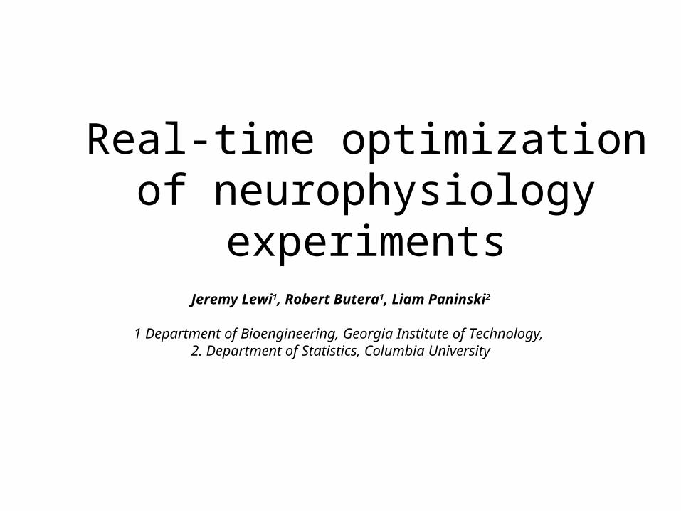
Neural Encoding

The neural code: what is P(response | stimulus)

Main Question: how to estimate P(r|x) from (sparse) experimental data?

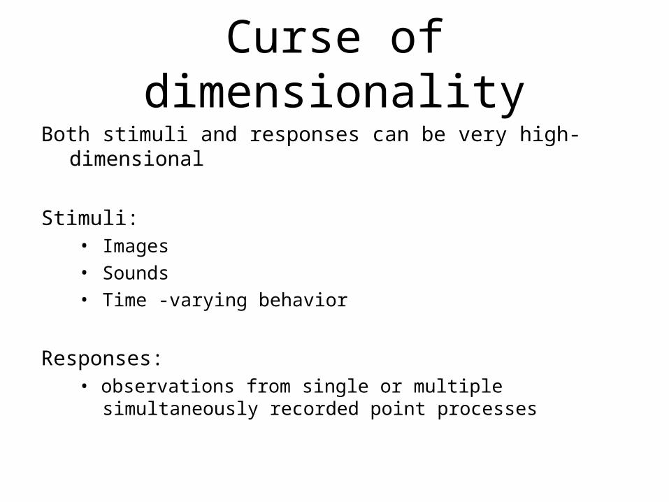
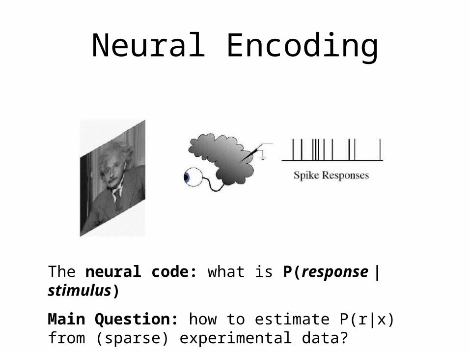
Curse of dimensionalityBoth stimuli and responses can be very high-dimensional

Stimuli:• Images• Sounds• Time -varying behavior

Responses:• observations from single or multiple simultaneously recorded

point processes

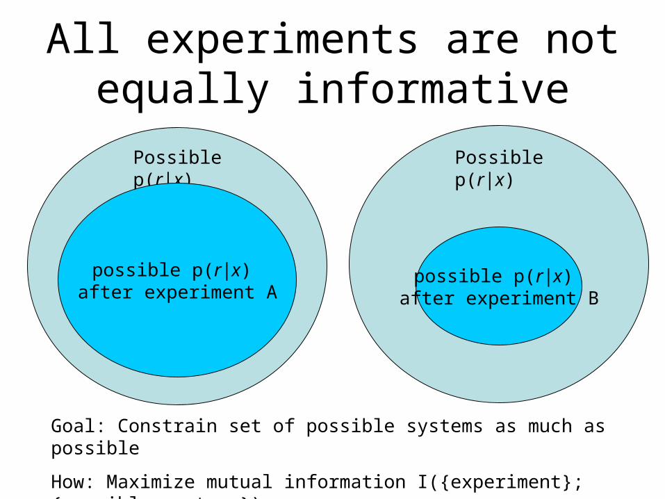
All experiments are not equally informative

Possible p(r|x)

possible p(r|x) after experiment A

Goal: Constrain set of possible systems as much as possible

How: Maximize mutual information I({experiment};{possible systems})

Possible p(r|x)

possible p(r|x) after experiment B

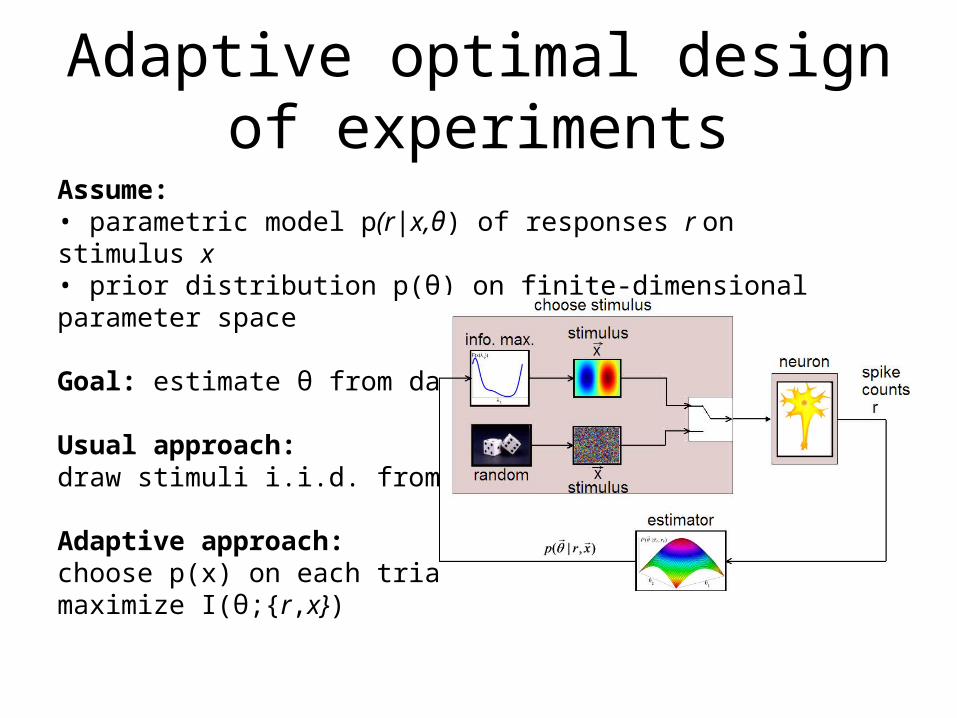
Adaptive optimal design of experiments

Assume:• parametric model p(r|x,θ) of responses r on stimulus x• prior distribution p(θ) on finite-dimensional parameter space

Goal: estimate θ from data

Usual approach: draw stimuli i.i.d. from fixed p(x)

Adaptive approach: choose p(x) on each trial to maximize I(θ;{r,x})

Theory: info. max is better1. Info. max. is in general more efficient and never worse than

random sampling [Paninski 2005]

2. Gaussian approximations are asymptotically accurate

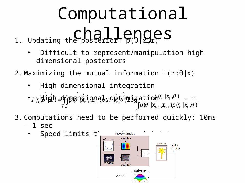
Computational challenges

),|(),|(

),|(log),|(),|()|;(

11

11

tttt

ttttt

r

tttxrpp

xrpxrppxrI

rxrx

3. Computations need to be performed quickly: 10ms – 1 sec• Speed limits the number of trials

1. Updating the posterior: p(θ|x,r)

• Difficult to represent/manipulation high dimensional posteriors

2. Maximizing the mutual information I(r;θ|x)

• High dimensional integration

• High dimensional optimization

Solution Overview

1. Model responses using a 1-d GLM• Computationally tractable

2. Approximate posterior as Gaussian • easy to work with even in high-d

3. Reduce optimization of mutual information to a 1-d problem

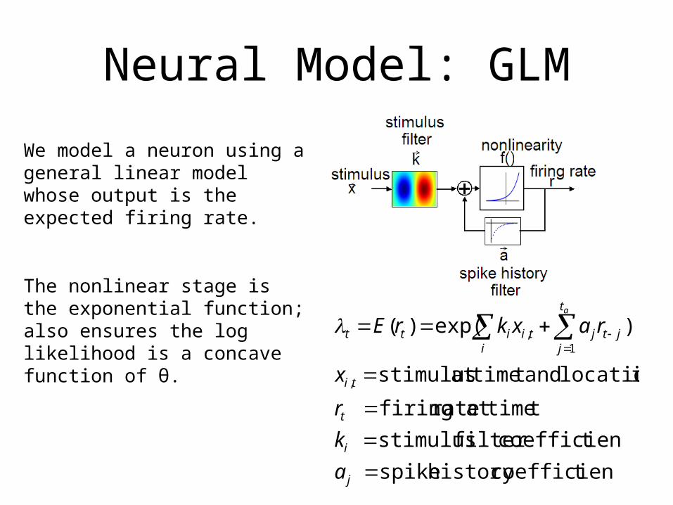
Neural Model: GLM

tcoefficienhistoryspike

tcoefficienfilterstimulus

ttimeatratefiring

ilocationandttimeatstimulus

)exp()(

,

1,

j

i

t

ti

i

t

jjtjtiitt

a

k

r

x

raxkrEa

We model a neuron using a general linear model whose output is the expected firing rate.

The nonlinear stage is the exponential function; also ensures the log likelihood is a concave function of θ.

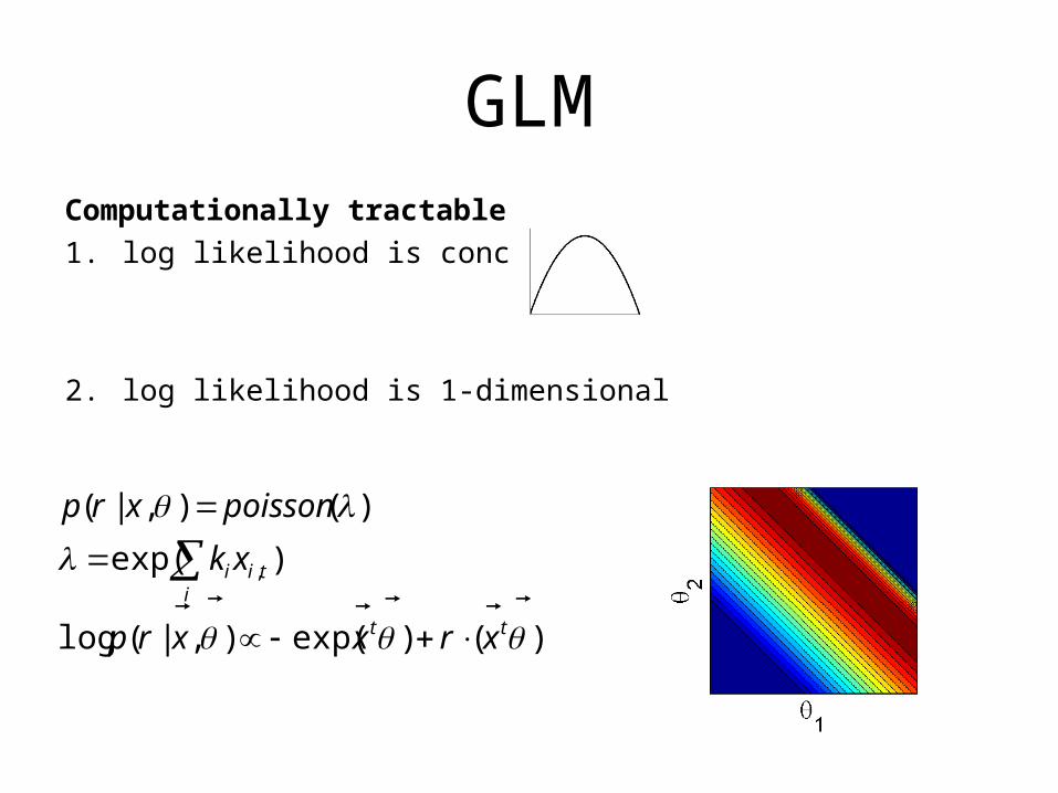
GLMComputationally tractable

1. log likelihood is concave

2. log likelihood is 1-dimensional

)()exp(),|(log

)exp(

)(),|(

,

tt

itii

xrxxrp

xk

poissonxrp

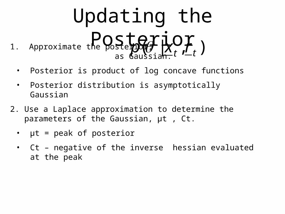
Updating the Posterior1. Approximate the posterior, as Gaussian.

• Posterior is product of log concave functions

• Posterior distribution is asymptotically Gaussian

2. Use a Laplace approximation to determine the parameters of the Gaussian, μt , Ct.

• μt = peak of posterior

• Ct – negative of the inverse hessian evaluated at the peak

),|( tt rxp

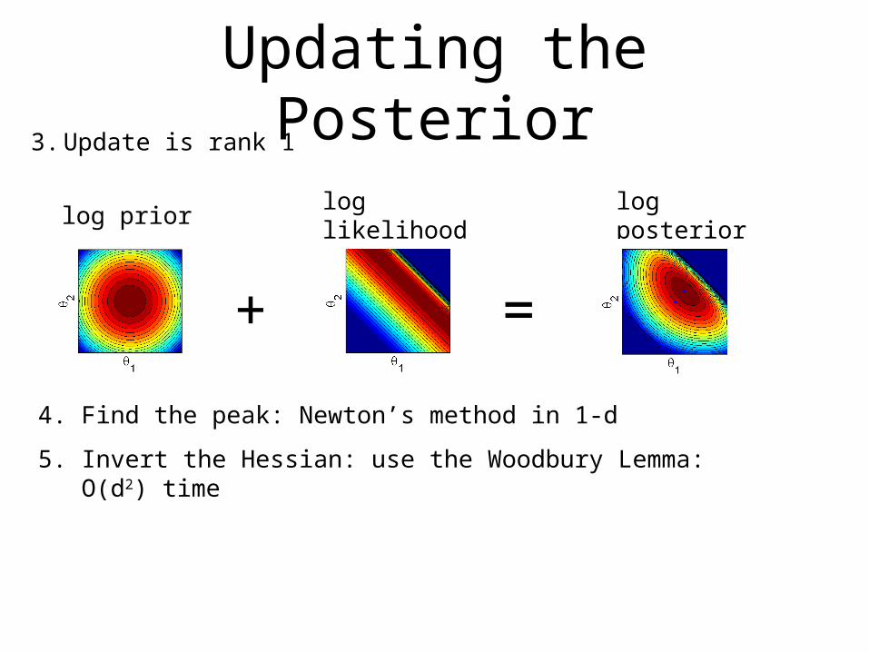
Updating the Posterior3. Update is rank 1

4. Find the peak: Newton’s method in 1-d

5. Invert the Hessian: use the Woodbury Lemma: O(d2) time

+ =

log prior log likelihood log posterior

Choosing the optimal stimulus• Maximize the mutual information Minimize the posterior entropy• Posterior is Gaussian:

• Compute the expected determinant– Simplify using matrix perturbation theory

• Result: Maximize an expression for the expected fisher information

• Maximization Strategy– Impose a power constraint on the stimulus– Perform an eigendecomposition– Simplify using lagrange multipliers– Find solution by performing a 1-d numerical optimization

• Bottleneck: Eigendecomposition – takes O(d2) in practice

||ln CEntropy

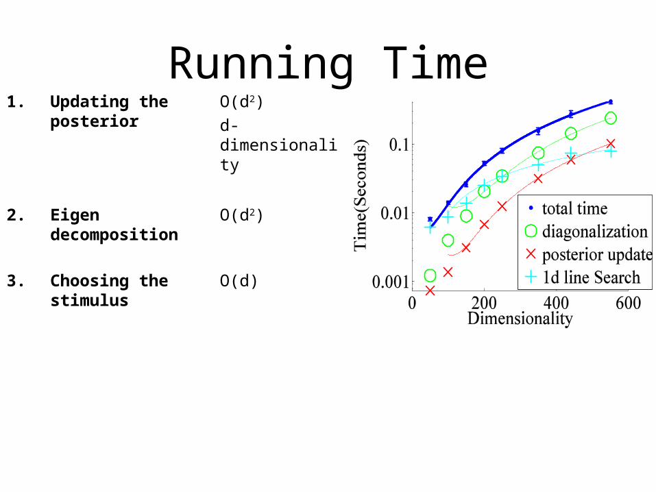
Running Time1. Updating the

posterior O(d2)

d- dimensionality

2. Eigen decomposition

O(d2)

3. Choosing the stimulus

O(d)

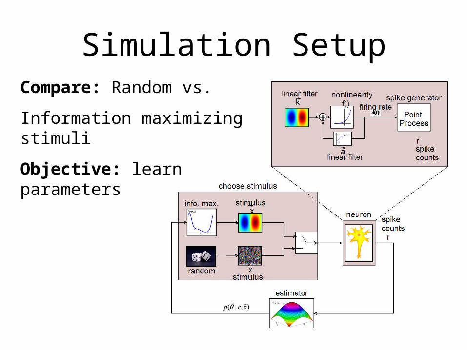
Simulation SetupCompare: Random vs.

Information maximizing stimuli

Objective: learn parameters

A Gabor Receptive Field

• high dimensional• Info. Max converges to true receptive field• Converges faster than random• 25x33

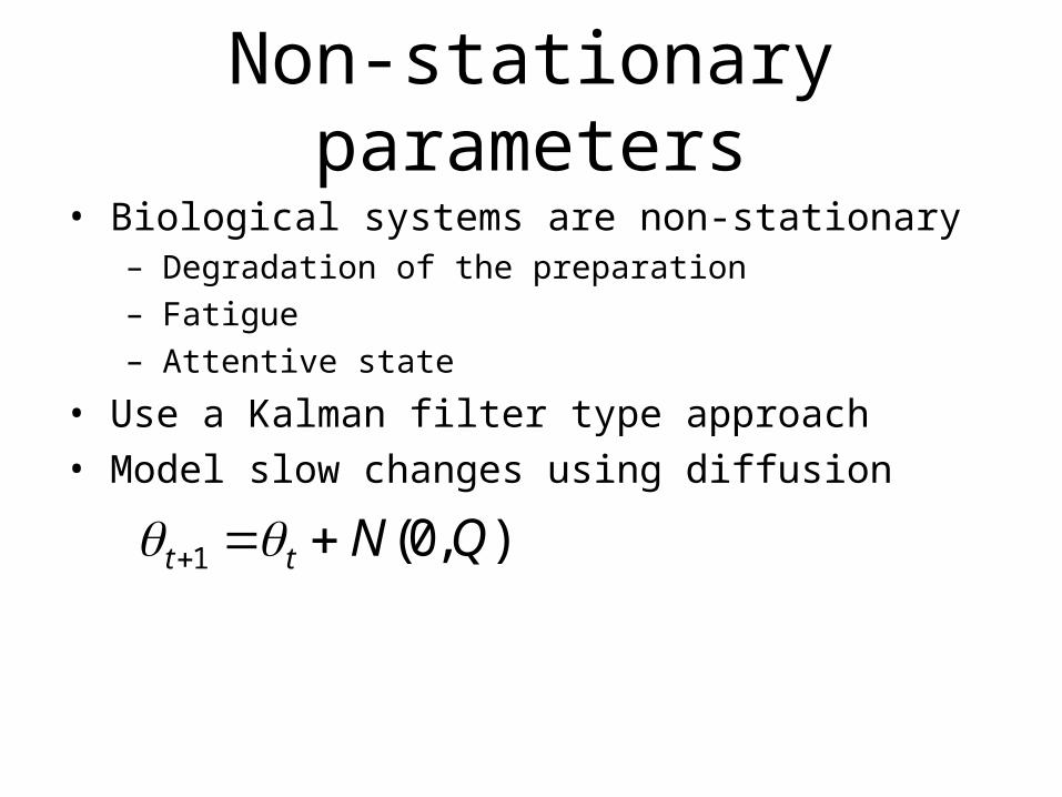
Non-stationary parameters

• Biological systems are non-stationary– Degradation of the preparation

– Fatigue

– Attentive state

• Use a Kalman filter type approach

• Model slow changes using diffusion

),0(1 QNtt

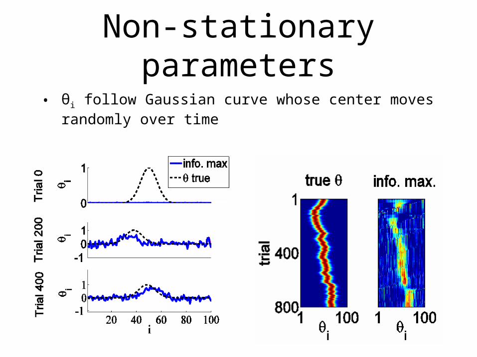
Non-stationary parameters

• θi follow Gaussian curve whose center moves randomly over time

• Assuming θ is constant overestimates certainty poor choices for optimal stimuli

Non-stationary parameters

Conclusions

1. Efficient implementation achievable with:1. Model based approximations

• Model is specific but reasonable

2. Gaussian approximation of the posterior• Justified by the theory

3. Reduction of the optimization to a 1-d problem

2. Assumptions are weaker than typically required for system identification in high dimensions

3. Efficiency could permit system identification in previously intractable systems

References1. A. Watson, et al., Perception and Psychophysics 33, 113 (1983).2. M. Berry, et al., J. Neurosci. 18 2200(1998)3. L. Paninski, Neural Computation 17, 1480 (2005).4. P. McCullagh, et al., Generalized linear models (Chapman and Hall, London, 1989).5. L. Paninski, Network: Computation in Neural Systems 15, 243 (2004).6. E. Simoncelli, et al., The Cognitive Neurosciences, M. Gazzaniga, ed. (MIT Press,

2004), third edn.7. M. Gu, et al., SIAM Journal on Matrix Analysis and Applications 15, 1266 (1994).8. E. Chichilnisky, Network: Computation in Neural Systems 12, 199 (2001).9. F. Theunissen, et al., Network: Computation in Neural Systems 12, 289 (2001).10. L. Paninski, et al., Journal of Neuroscience 24, 8551 (2004)

AcknowledgementsThis work was supported by the Department of Energy Computational

Science Graduate Fellowship Program of the Office of Science and National Nuclear Security Administration in the Department of Energy under contract DE-FG02-97ER25308 and by the NSF IGERT Program in Hybrid Neural Microsystems at Georgia Tech via grant number DGE-0333411.

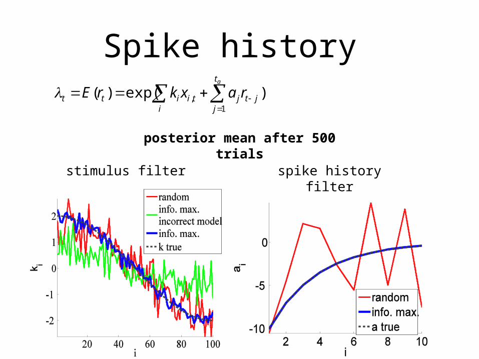
Spike history

i

t

jjtjtiitt

a

raxkrE1

, )exp()(

posterior mean after 500 trials

stimulus filter spike history filter

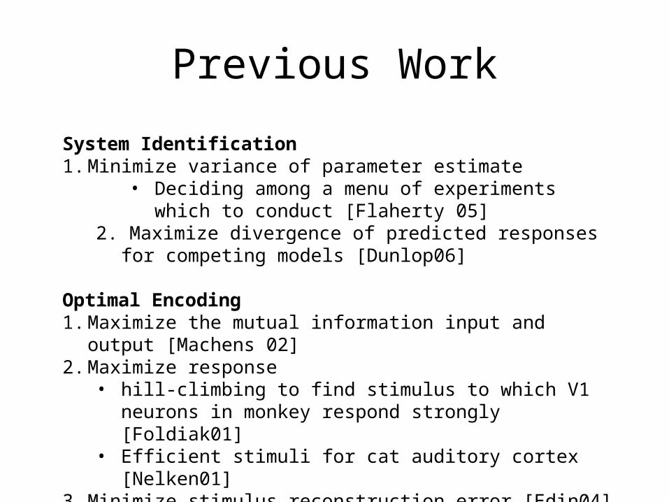
Previous Work

System Identification1. Minimize variance of parameter estimate

• Deciding among a menu of experiments which to conduct [Flaherty 05]

2. Maximize divergence of predicted responses for competing models [Dunlop06]

Optimal Encoding1. Maximize the mutual information input and output [Machens 02]2. Maximize response

• hill-climbing to find stimulus to which V1 neurons in monkey respond strongly [Foldiak01]

• Efficient stimuli for cat auditory cortex [Nelken01]3. Minimize stimulus reconstruction error [Edin04]

Derivation of Choosing the Stimulus I

111

11

1|1

1111

11

)),((

]det[log2

1),|(

),|(),|(),,|;(

),,|;(maxarg

11

1

ttobstt

txrtt

tttttttt

ttttx

xrJCC

constCErxH

rxHrxHrxxrI

rxxrI

tt

t

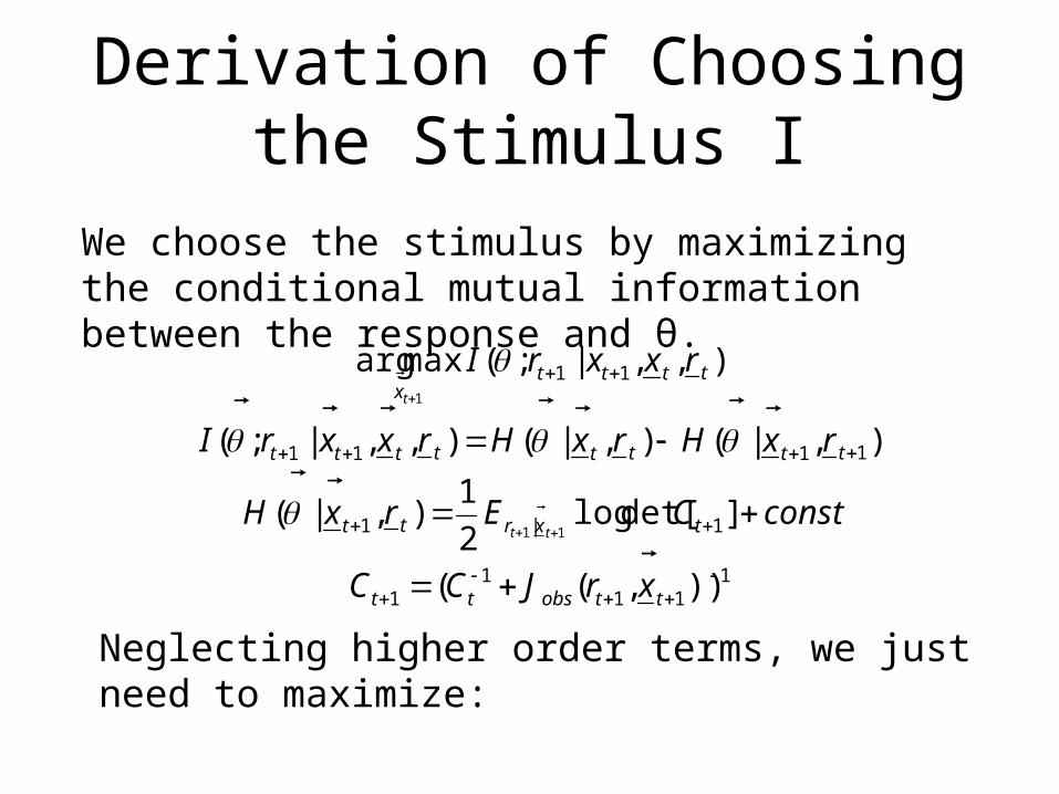
We choose the stimulus by maximizing the conditional mutual information between the response and θ.

Neglecting higher order terms, we just need to maximize:

Derivation of Choosing the Stimulus II

tobsttttobst CJCCxrJC

111

1 )),((

)(][

]|log~]|log

tobstobsr

tobsrtobsttr

CJoCJtrE

CJIECJCCE

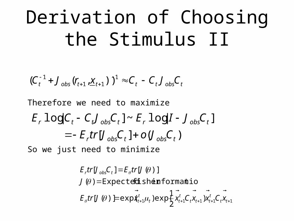
So we just need to minimize

Therefore we need to maximize

11111 )2

1exp()exp()]([

ninformatiofisher Expected)(

)]([][

tttttt

ttt

tt

tobsr

xCxxCxxJtrE

J

JtrECJtrE

Maximization

i

iii

iii

iit ycycyuxF 221 )

2

1exp()exp()(

We maximize the above subject to a power constraint by breaking it up into an inner and outer problem.

])2

1exp(maxarg[)exp(maxarg)(maxarg 22

,||:||1

21 iii

iii

buyeyybt

X

ycycbXFt

t

To maximize this expression, we express everything in terms of the eigenvectors of Ct..

are the projection of the mean and stimulus onto the eigenvectors.

yu

,

111111 )2

1exp()exp()()]([ tt

tttt

ttt

ttt xCxxCxxxFJtrE

Maximization II

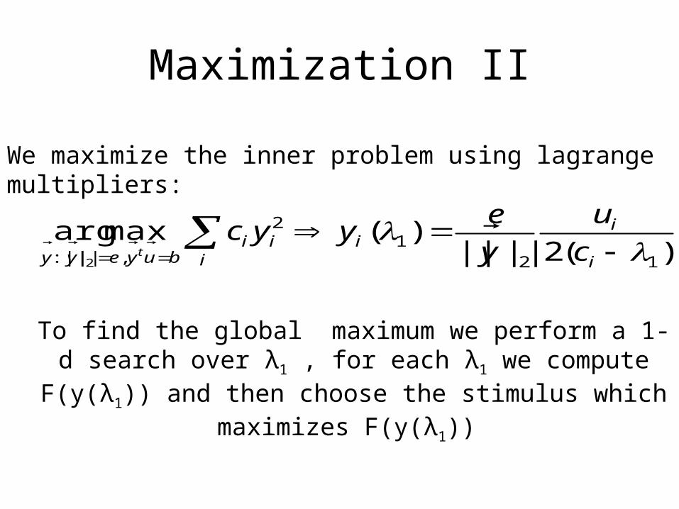
We maximize the inner problem using lagrange multipliers:

)(2||||)(maxarg

121

2

,||:|| 2

i

ii

iii

buyeyy c

u

y

eyyc

t

To find the global maximum we perform a 1-d search over λ1 , for each λ1 we compute F(y(λ1)) and then choose the

stimulus which maximizes F(y(λ1))

Posterior Update: Math

t

t

t

t

t

t

t

t

ttt r

x

r

x

r

xCC

111

11

1 )exp(

t

t

t

t

t

tt

t

t

ttt

tt

t

t

tt

t

t

ttt

ttt

r

x

r

xr

r

xC

d

xrpd

r

xr

r

xC

t

t

111

11

111

11

)exp()(),|(log

)exp()()(2

1maxarg

1

1