Real-Time Motion Control Using Pose Space Probability Density Estimation

Dumebi Okwechime, Eng-Jon Ong, and Richard BowdenCVSSP, University of Surrey, Guildford, Surrey, GU17XH, UK

{d.okwechime,e.ong,r.bowden}@surrey.ac.uk

AbstractThe ability to control the movements of an object or

person in a video sequence has applications in the movieand animation industries, and in HCI. In this paper, we in-troduce a new algorithm for real-time motion control anddemonstrate its application to pre-recorded video clips andHCI. Firstly, a dataset of video frames are projected intoa lower dimension space. A k-mediod clustering algorithmwith a distance metric is used to determine groups of simi-lar frames which operate as cut points, segmenting the datainto smaller subsequences. A multivariate probability dis-tribution is learnt and probability density estimation is usedto determine transitions between the subsequences to de-velop novel motion. To facilitate real-time control, condi-tional probabilities are used to derive motion given usercommands. The motion controller is extended to HCI us-ing speech Mel-Frequency Ceptral Coefficients (MFCCs) totrigger movement from an input speech signal. We demon-strate the flexibility of the model by presenting results rang-ing from datasets composed of both vectorised images and2D point representation. Results show plausible motiongeneration and lifelike blends between different types ofmovement.

1. Introduction

Video synthesis has been an emerging topic in recent

years, highly applicable to the movie and games industries.

When filming a movie, certain elements in a video scene

such as the movement of trees blowing in the wind, do not

perform on cue. It may not always be cost effective, safe

or even possible to control the surroundings to match the

directors intentions. In this paper, an approach to control-

ling pre-recorded motions in a video clip is presented giving

the user real-time control in creating novel video seqences.

This is achieved by modelling the motion in the video se-

quence as a pose space probability density function (PDF).

The model can synthesize novel sequences whilst retaining

the natural variances inherit to the original data. By learning

the mapping between motion subspaces and external stimu-

Figure 1. Images showing candle and plasma beam videos.

Figure 2. Images showing tracked face data used in modelling con-

versational cues.

lus, the user can drive the motion at an intuitive level.

As an extension to this work, the system is also demon-

strated in modelling human conversational cues in a social

context. During a one to one conversation, listeners tend

to infer their engagement by nodding or performing some

sort of non-verbal behaviour. These responses are in most

cases encouraged by the speaker’s tone. When a speaker at-

tempts to make a point, they put emphasis on certain words

which is a cue for the listener to acknowledge with some vi-

sual gesture. Here, having learnt their relationship, we take

visual and audio features captured in a social context and

synthesize appropriate, novel responses to audio stimulus.

Our Motion Control Model has four stages. First, given

a dataset of video frames, the data is projection to a lower

dimension pose space using Principal Component Analysis

(PCA). Next, the space is segmented into cut points using

2056 2009 IEEE 12th International Conference on Computer Vision Workshops, ICCV Workshops 978-1-4244-4441-0/09/$25.00 ©2009 IEEE

an unsupervised k-mediod clustering algorithm. These cut

points represent points in the video sequence where a tran-

sition to a different subsequence is possible. We model the

data in pose space using a PDF where motion is generated

as the likelihood of a transition given a cut point. Finally,

a real-time motion control system is developed mapping a

user interface to the desired movement. Figure 1 shows the

candle flame and plasma beam sequences used for video

textures. The purpose of the Motion Control Model is to

control the direction which the flame and beam move in

real-time whilst generating a novel animation with plausi-

ble transitions between different types of movement. Fig-

ure 2 shows a 2D tracked contour of a face generated from

a video sequence of a person listening to a speaker. Map-

ping the audio MFCC features of the speaker to the 2D face,

we generate appropriate non-verbal responses triggered by

novel audio input.

The paper is divided into the following sections. Sec-

tion 2, briefly details related works in the field of video

data modelling and motion synthesis. Section 3 presents an

overview of the Motion Control System. Secton 4 details the

technique used for learning the model. Section 5 presents

the real-time motion control system and the remainder of

the paper describes the results and conclusions are drawn.

2. Related WorkThere are several techniques to synthesizing video. Early

approaches were based on parametric [6] [18] and non-

parametric [4] [21] texture synthesis methods which cre-

ate novel textures from example inputs. Kwatra et al. [9]

generate perceptually similar patterns from smaller train-

ing data using a graph cut technique based on Markov Ran-

dom Fields (MRF). Bhat et al. [2] presents an alternative ap-

proach to synthesize and edit videos by capturing dynamics

and texture variation using texture particles traveling along

user defined flow lines. Schodl et al. [16] introduces VideoTextures which computes the distances between frames to

derive appropriate transition points to generate a continu-

ous stream of video images from a small amount of training

video. The limitation to this approach is, to determine tran-

sition points, frame-to-frame distances are calculated for all

frames which can be computationally expensive for large

data sets. Also, their dynamic programming algorithm only

allows for backward transitions limiting the scope of poten-

tial transitions.

In this work, we look at video synthesis as a continuous

motion estimation problem, inspired by techniques used in

modelling motion captured data. Troje [20] was one of the

first to use a simple sine functions to model motion. Pullen

and Bregler [14] used a kernel based probability distribution

to extract ’motion texture’ i.e. the personality and realism,

from the motion capture data to synthesize novel motion

with the same style and realism of the original data. Ok-

wechime and Bowden [12] extended this work using a mul-

tivariate probability distribution to blend between different

types of cyclic motion to create novel movement. Arikan

et al. [1] allow a user to synthesize motion by creating a

timeline with annotationed instructions such as walk, run

or jump. For this approach to be successful, a relatively

large database is needed to work with their optimisation

technique otherwise it may result in highly repetitive mo-

tion generation.

Treuille et al. [19] developed a system that synthesizes

kinematic controllers which blend subsequences of precap-

tured motion clips to achieve a desired animation in real-

time. The limitation to this approach is it requires manual

segmentation of motion subsequences to a rigid design in

order to define appropriate transition points. Our motion

control model uses an unsupervised k-mediod algorithm for

sequence segmention and extends the application of motion

modelling to generate novel motion sequences in video.

In Human Computer Interaction (HCI), using audio fea-

tures to drive a model can be a useful tool in developing

effective user interfaces. Brand [3] learns a facial control

model driven by audio speech signals to produce realistic

facial movement including lip-syncing and upper-face ex-

pressions. Stone et al. [17] uses context dependent scripts

to derive an animation’s body language including hand ges-

tures. In these examples, audio signals are used to animate

a speaker but little work has looked at using audio signals to

animate a listener in a conversational context in real-time.

Jebara and Pentland [7] touched on modelling conversa-

tional cues and proposed Action Reaction Learning (ARL),

a system that generates an animation of appropriate hand

and head poses in response to a users hand and head move-

ment in real-time. However, this does not incorporate audio.

In this paper, we demonstrate the flexibility of the motion

controller, modelling conversation cues based on audio in-

put. Audio features of the speaker, represented by MFCCs,

are used to derive appropriate visual responses of the lis-

tener in real-time from a 2D face contour modelled with the

motion controller. This results in plausible head movement

and facial expressions in response to the speaker’s audio.

3. System OverviewThe purpose of the Motion Control System is to learn a

model of a single agent undergoing motion. The model will

allow a user to reproduce motion in a novel way by specify-

ing in real-time which type of motion to perform inherent in

the original sequence. This is achieved by learning a posespace PDF.

We start by creating a first order dynamic representation

of the motion in pose space. Then, using conditional proba-

bilities we are able to dynamically change likelihoods of the

pose to give the user control over the final animation. This

is demonstrated in three examples:

2057

Figure 3. (A) Plot of eigen projection of first 2 dimensions of a

candle video sequence, (B) Image showing k-mediod points num-

bered, (C) Image showing cut point groups in eigenspace, (D) Im-

age showing transitions between cut points.

• Candle Flame. We synthesize the movement of a can-

dle flame where the user has control over three dis-

crete states: ambient flame, flame blow left, flame blowright, and can blend between them.

• Plasma Beam. The user controls the movement of a

plasma beam using conditional probability to provide

a continuous user interface.

• Tracked 2D Face Contour. An animation of a 2D

face is driven directly from an audio signal, displaying

appropriate visual responses for an avid listener based

on audio stimulus.

4. Motion Control ModelThere are several stages involved in developing the Mo-

tion Control Model. Given a data set of an agent undergo-

ing motion, the frames are vectorised and dimensionally re-

duced for efficiency. An unsupervised clustering algorithm

is then used to segment the data into smaller segments. This

leads to the computation of the pose space PDF on the data

on which the motion model is derived. A kd-tree is used for

rapid density estimation and dynamic programming is used

to estimate novel transitions between segments in the data,

based upon the influence of a user in terms of probability

of desired appearance. Conditional Probabilities map from

the input space to that of synthesis, providing the user with

control over the final animation.

4.1. Data

Given the motion sequence X, each frame is represented

as a vector xi where X = {x1, ..., xF } and F is the num-

ber of frames. Various motion data formats can be used in

this system. So far, both 2D tracked points and rgb pix-

els have been successfully implemented. In both cases,

each time step i of the data to be modelled is vectorised

as xi = (xi1, yi1, ..., xin, yin) ∈ �2n for a 2D contour of npoints or xi = (r11, g11, b11, ..., rxy, gxy, bxy) ∈ �xy for an

x × y image.

4.2. Eigenspace Representation

To reduce the complexity of building a generative model

of motion, Principal Component Analysis (PCA) [15] is

used for dimensionality reduction.

For a given D-dimension data set X, as defined in Section

4.1, the D principal axes T1, T2, ..., TD are given by the Dleading eigenvectors of the sample covariance matrix S. An

eigen decomposition gives S =∑

λiTi, i ∈ {1, ..., D},where λi is the ith largest eigenvalue of S.

The dimension of the feature space is reduced by pro-

jecting into the eigenspace

yi = VT (xi − μ) (1)

where μ is the sample mean μ = 1F

∑Fi=1 xi, V are the

eigenvectors V = [T1, ..., Td] and d is the chosen lower

dimension d ≤ D such that∑d

i=1λi

Σ∀λ ≥ .95 or 95% of

the energy is retained. Y is defined as a set of all points

in the dimensionally reduced data where Y = {y1, ..., yF }and yi ∈ �d. This results in a d-dimension representation

of each frame in the sequence. This representation reduces

the computational and storage complexity of the data whilst

still retaining the time varying relationships between each

frame. Figure 3 (A) shows a plot of the candle data set

projected onto the first two eigenvectors. It produces a non-

linear but continuous sub-space characteristic of continuous

motion.

4.3. Unsupervised Segmentation

As explained in the introduction to Section 4, this

lower dimension data is segmented into several short sub-

sequences. A single subsequence is represented as a set of

consecutive frames between a start and end transition point.

The idea is to connect various subsequences together to cre-

ate a novel sequence.

Figure 4 shows an example of the process of unsuper-

vised segmentation. To cut the data into smaller segments

and derive subsequences with appropriate start and end tran-

sition points, various points of intersection in the motion

trajectory, which we refer to as cut points, need to be deter-

mined. Given a motion sample, shown by the two dimen-

sion motion trajectory in Figure 4 (A), a k-mediod cluster-

ing algorithm is used to find Nc k-mediod points. K-mediod

points are data points derived as cluster centre in regions of

high density. In Figure 4 (B), Nc = 3 and are shown as the

three red crosses which we refer to as a, b, and c. Using a

2058

Figure 4. (A) Trajectory of the original motion sequence. Arrows indicate the direction of motion. (B) Nc = 3 k-mediod points derived

using the unsupervised k-mediod clustering algorithm. The three red crosses are the three k-mediod points a, b, and c. (C) The small green

dots are the cut points derived as the nearest neighbouring points to a k-mediod point less than a user defined threshold θ. The three gray

circles represent cut point groups a, b and c. (D) Cut points act as start and end transition points segmenting the data into shorter segments.

The orange dots are start transition points and the purple dots are end transition points. (E) Diagram of possible transitions within group c.

For simplicity only a few transitions are displayed.

distance matrix, the nearest neighbouring points to each k-

mediod points are derived and make up groups of cut points.

The cut points are represented by the small green dots in 4

(C), and the groups of cut points are represented by the gray

circles. Cut point groups consists of discrete frames which

are not directly linked, however smooth transitions can be

made between them. Similar to Motion Graphs [8], an ap-

proach used in character animation, assuming frames close

to each in eigenspace are similar, a simple blending tech-

niques such as linear interpolation can reliably generate a

transition. As shown in Figure 4 (D) the cut point are used

to segment the data to smaller subsequences with start and

end transition points. 4 (E) shows a few of the possible tran-

sitions between various subsequences in group c.

Firstly, we define a database distance matrix D to de-

termine the similarity between all frames in the video se-

quence.

D(i,j) = d(yi, yj)|i = {1, ..., F}, j = {1, ..., F} (2)

The distance between the frames can be calculated by com-

puting the L2 distance between their corresponding points

in eigenspace.

The next step is to cluster the data to estimate suitable

cut points using an unsupervised k-mediod clustering algo-

rithm. The k-mediod clustering algorithm works similarly

to the k-means clustering algorithm in that it associates to

each cluster the set of images in the database that closely

resembles the cluster centre. The main difference is that

the cluster centre is represented as a data point median as

opposed to a mean in the eigenspace. This ensures that no

blurring occurs and all points are embedded within the data.

We define Nc k-mediod cluster centres as μci given by

the k-mediod method whereby μci ∈ Y and 0 < i < Nc.

The set containing the members of the nth cluster is defined

as Ycn = {yc

n,1, ..., ycn,Cn

}, where the number of members

of the nth cluster is denoted as Cn.

Figure 3 (B) shows a set of Nc = 36 k-mediod points

used for the candle video synthesis. Nc is chosen based

on the number of clusters that best defines the distribution

of poses in pose space. If Nc is too high, the model will

generate unrealistic motion and if Nc is too low, not enough

cut points will be available to provide transitions to varying

motion types reducing the novelty of animation.

Cut points are data points where the distance to μci is less

than threshold θ. The threshold is determined experimen-

tally whereby if it is set to high, it becomes more challeng-

ing to produce plausible blends when making transitions,

and if its too low, potential cut points are ignored and we

are limited to points that overlap, which is an unlikely oc-

curance in a multi-dimensional space.

As shown in Figure 3 (C), we are able to represent the

data as cut point groups where transitions between subse-

quences are generated by branching cut points, as demon-

strated in Figure 3 (D). Cut point groups represent groups

of frames where, via simple linear interpolation, a transi-

tion to a different subsequence can occur. Taking Yci =

{yci,1, yc

i,2, yci,3} as a set of neighbouring cut points as illus-

trated in Figure 5. If a transition is made to yci,1, since yc

i,1

is in the same group as yci,2 and yc

i,3, they are consider close

enough in pose space to create a visually plausible blend.

If the next desired subsequence is a transition from yci,3 to

yca,α, the model blends from pose yc

i,1 to yci,3 using linear

interpolation, then the transition is made to yca,α.

4.4. Appearance Model

4.4.1 Pose Space PDF

A PDF of appearance is created using kernel estimation

where each kernel p(yi) is effectively a Gaussian centred

on a data example p(yi) = G(yi, Σ). Since we want our

2059

Figure 5. Image showing transitions between cut points in different

clusters where α is any cut point member in its respective group.

probability distribution to represent the dimensionally re-

duced data set Y of d dimensions as noted in Section 4.2,

the likelihood of a pose in pose space is modelled as a mix-

ture of Gaussians using multivariate normal distributions.

We will refer to this Gaussian mixture model as the posespace PDF.

P (y) =1F

F∑i=1

p(yi) (3)

where the covariance of the Gaussian is:

Σ = α

⎛⎜⎝√

λ1 · · · 0...

. . ....

0 · · · √λd

⎞⎟⎠ (4)

For these experiments α = 0.5.

4.4.2 Fast Gaussian Approximation

As can be seen from Equation 3, the computation required

for the probability density estimation is high since it re-

quires an exhaustive search through the entire set of data ex-

amples. This causes slow computation for real time imple-

mentation. As a result, a fast approximation method based

on kd-trees [11] is used to reduce the estimation time with-

out sacrificing accuracy.

Instead of computing kernel estimations based on all data

points, with the kd-tree we can localise our query to neigh-

bouring kernels, assuming the kernel estimations outside a

local region contribute nominally to the local density esti-

mation. We are now able to specify Nn nearest neighbours

to represent the model, where Nn < NT . This significantly

reduces the amount of computation required. Equation 3 is

simplified to:

P (y) =1

Nn

Nn∑i=1

p(yi) (5)

where yi are the Nn nearest neighbouring kernels found

efficiently with the kd-tree, and yi ∈ Y.

4.4.3 Markov Transition Matrix

When generating novel motion sequences, we are not only

interested in generating the most likely pose/frame but also

the mostly probable path leading to it. A first order Markov

Transition Matrix [5] is used to discourage movements that

are not inherent in the training data. As an approach for-

mally used with time-homogeneous Markov chains to de-

fine transition between states, by treating our clusters of cut

points Yci as states, this approach can be used to apply fur-

ther constraints and increase the accuracy of the transition

between sequences.

We define Pk,l = {pkl} as the transition matrix whereby

Pk,l denotes the fixed probability of going from cluster k to

cluster l, and∑

l Pk,l = 1. We are now able to represent

the conditional probability of moving from one cluster to

another as P (Ct|Ct−1) = Pt−1,t where Ct is defined as

the index for a cluster/state at time t. This transition matrix

is constructed using the cut points within the sequence to

identify the start and end transitions within the data.

The transition matrix probability values act as weighting

variables, giving higher influence to transitions that occur

more frequently in the original data. To account for situ-

ations where the only possible transition is highly improb-

able, a uniform normalisation value υ = 0.5 is added to

all elements in the transition matrix before normalisation.

This allows the transition model to move between states not

represented as transitions in the original sequence.

4.4.4 Generating Novel Video Sequences

To generate novel motion sequences the procedure is:

1. Given the current position in pose space yt, find all

adjacent cut points and associate transition sequences.

The end points of these sequences gives a set of Mpossible modes in pose space {y1

t+1, ..., yMt+1}

2. Derive cluster index Ci,t for yt (where yt ∈ Yci,t), and

its corresponding future cluster indices (Cmi,t+1)∀m

where ymt+1 ∈ Yc

i,t+1.

3. Calculate the likelihood of each mode as:

φm = P (Cmi,t+1|Ci,t)P (ym

t+1) (6)

where Φ = {φ1, ..,φM}.4. Randomly select a sequence from Φ based upon its

likelihood.

2060

5. Using Linear interpolation, blend yt to the new se-

quence start.

6. The frames associated to transition sequence are re-

constructed for rendering as xt = (μ + Vyt).

7. The process then repeats from step (1).

4.4.5 Dynamic Programming

Similar to a first order markov chain, our goals are currently

in terms of the next step in the transition. In most cases, mo-

tion requires sacrificing short term objectives for the longer

term goal of producing a smooth and realistic sequence. As

a result, dynamic programming is used for forward plan-

ning. Formally used in Hidden Markov Models to deter-

mine the most likely sequence of hidden states, it is applied

to the pose space PDF to observe the likelihoods for m = 3steps in the future.

Treating our clusters as states, a trellis is built m steps in

the future effectively predicting all possible transitions mlevels ahead. Dynamic programming is then used to find

the most probable path for animation.

5. Real-Time Motion Control SystemThus far, the Motion Control Model randomly generates

the mostly likely set of motion sequences given a starting

configuration. To allow real-time control of the motions we

use a Projection Mapping method.

5.1. Projection Mapping

The Projection Mapping approach is used when wanting

to enable motion control using an interface such as a mouse

cusor, touch screen monitor or even on audio features.

The input space is quantised into an appropriate number

of symbols. Using the direct mapping within the training

data of input symbols and the clusters of the pose space, a

condition probability is calculated that maps from the input

space to pose space P (C|input). This is used at run-time

to weight the pose space PDF in the motion controller by

altering Equation 5 to:

P (y) =1

Nn

Nn∑i=1

p(yi)ω (7)

where

ω ={

P (Ci|input) if yi ∈ Yci

0 otherwise (8)

6. Experimental ResultsTo produce our results we performed tests on three dif-

ferent data sets. Two data sets consist of video sequences,

and the other consists of a video and audio recording of two

people in a conversation with each other.

6.1. Experiments with Video Data

Two video sequences were recorded using a webcam of a

single agent performing various types of motion. One was

of a candle flame and the other of plasma beams from a

plasma ball. The candle flame sequence was captured using

a webcam (185 × 140 pixels, 15 frames per second). The

recording was 3:20 minutes long containing 3000 frames.

Similarly the plasma beam sequence was captured with a

webcam (180 × 180 pixels, 15 frames per second). The

recording was 3:19 minutes long containing 2985 frames.

The candle flame sequence consists of the candle perform-

ing 3 different motions, blowing left, blowing right and

burning in a stationary position. The plasma beam sequence

however has more varying movement, from multiple ran-

dom plasma beams too a concentrated beam from a point of

contact around the edges of the ball.

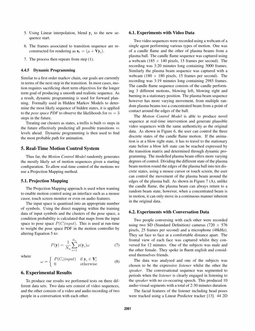
The Motion Control Model is able to produce novel

sequence at real-time intervention and generate plausible

video sequences with the same authenticity as the original

data. As shown in Figure 6, the user can control the three

discrete states of the candle flame motion. If the anima-

tion is at a blow right state, it has to travel to the stationary

state before a blow left state can be reached expressed by

the transition matrix and determined through dynamic pro-

gramming. The modelled plasma beam offers more varying

degrees of control. Dividing the different state of the plasma

beam motion round the edges of the plasma ball into ten dis-

crete states, using a mouse cursor or touch screen, the user

can control the movement of the plasma beam around the

edges of the plasma ball. As shown in Figure 7 (A), unlike

the candle flame, the plasma beam can always return to a

random beam state, however, when a concentrated beam is

in motion, it can only move in a continuous manner inherent

in the original data.

6.2. Experiments with Conversation Data

Two people conversing with each other were recorded

using two SD (Standard Definition) cameras (720 × 576

pixels, 25 frames per second) and a microphone (48kHz).

They sat face to face at a comfortable distance apart. The

frontal view of each face was captured whilst they con-

versed for 12 minutes. One of the subjects was male and

the other female. They spoke in fluent english and consid-

ered themselves friends.

The data was analysed and one of the subjects was

chosen to be the expressive listener whilst the other the

speaker. The conversational sequence was segmented to

periods when the listener is clearly engaged in listening to

the speaker with no co-occuring speech. This produced 10

audio-visual segments with a total of 2:30 minutes duration.

The facial features of the listener including head poses

were tracked using a Linear Predictor tracker [13]. 44 2D

2061

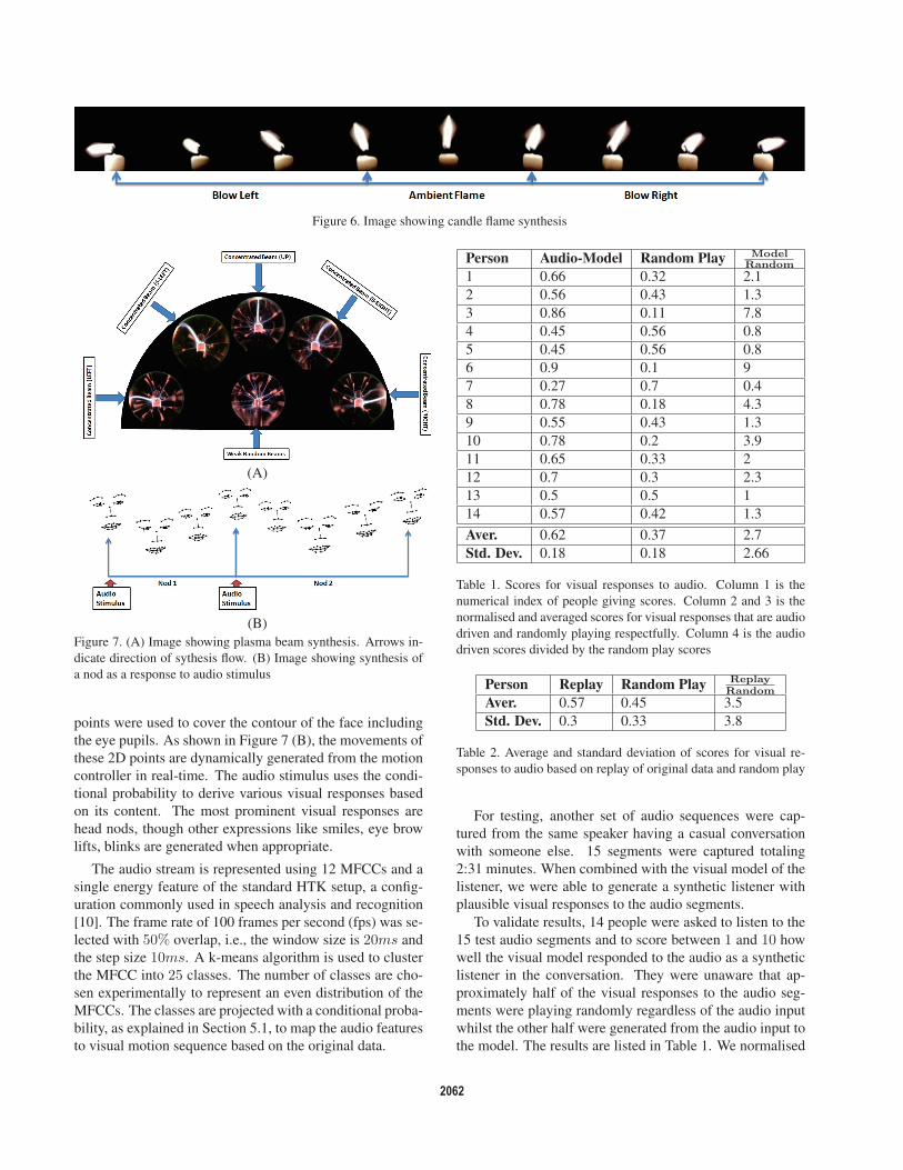
Figure 6. Image showing candle flame synthesis

(A)

(B)

Figure 7. (A) Image showing plasma beam synthesis. Arrows in-

dicate direction of sythesis flow. (B) Image showing synthesis of

a nod as a response to audio stimulus

points were used to cover the contour of the face including

the eye pupils. As shown in Figure 7 (B), the movements of

these 2D points are dynamically generated from the motion

controller in real-time. The audio stimulus uses the condi-

tional probability to derive various visual responses based

on its content. The most prominent visual responses are

head nods, though other expressions like smiles, eye brow

lifts, blinks are generated when appropriate.

The audio stream is represented using 12 MFCCs and a

single energy feature of the standard HTK setup, a config-

uration commonly used in speech analysis and recognition

[10]. The frame rate of 100 frames per second (fps) was se-

lected with 50% overlap, i.e., the window size is 20ms and

the step size 10ms. A k-means algorithm is used to cluster

the MFCC into 25 classes. The number of classes are cho-

sen experimentally to represent an even distribution of the

MFCCs. The classes are projected with a conditional proba-

bility, as explained in Section 5.1, to map the audio features

to visual motion sequence based on the original data.

Person Audio-Model Random Play ModelRandom

1 0.66 0.32 2.1

2 0.56 0.43 1.3

3 0.86 0.11 7.8

4 0.45 0.56 0.8

5 0.45 0.56 0.8

6 0.9 0.1 9

7 0.27 0.7 0.4

8 0.78 0.18 4.3

9 0.55 0.43 1.3

10 0.78 0.2 3.9

11 0.65 0.33 2

12 0.7 0.3 2.3

13 0.5 0.5 1

14 0.57 0.42 1.3

Aver. 0.62 0.37 2.7

Std. Dev. 0.18 0.18 2.66

Table 1. Scores for visual responses to audio. Column 1 is the

numerical index of people giving scores. Column 2 and 3 is the

normalised and averaged scores for visual responses that are audio

driven and randomly playing respectfully. Column 4 is the audio

driven scores divided by the random play scores

Person Replay Random Play ReplayRandom

Aver. 0.57 0.45 3.5

Std. Dev. 0.3 0.33 3.8

Table 2. Average and standard deviation of scores for visual re-

sponses to audio based on replay of original data and random play

For testing, another set of audio sequences were cap-

tured from the same speaker having a casual conversation

with someone else. 15 segments were captured totaling

2:31 minutes. When combined with the visual model of the

listener, we were able to generate a synthetic listener with

plausible visual responses to the audio segments.

To validate results, 14 people were asked to listen to the

15 test audio segments and to score between 1 and 10 how

well the visual model responded to the audio as a synthetic

listener in the conversation. They were unaware that ap-

proximately half of the visual responses to the audio seg-

ments were playing randomly regardless of the audio input

whilst the other half were generated from the audio input to

the model. The results are listed in Table 1. We normalised

2062

each person’s score and took the average for both audio-

model generation and random play. As shown in the fourth

column of Table 1 entitled ‘ ModelRandom ’, 11 out of 14 gener-

ated a score greater than or equal to 1, showing preference

to the visual responses generated by the audio input than by

the random play. Although the majority could tell the dif-

ference, the margins of success are not considerably high

producing an average of 0.62. Several assumptions may be

drawn from this. As nods are the most effective non-verbal

responses of an engaged listener, random nods can be an ac-

ceptable response to a speaker. To try to validate these tests,

the same 14 people were asked to repeat the test but this

time on the 10 audio segments used in training the model.

5 out of 10 of the audio segments were randomly playing

visual response and the other 5 were replays of the origi-

nal audio-visual pairing. Results in Table 2 show that most

people prefer the replay to the random play visual responses

but with a similar margin of success when compared to our

model generation. The test with the real data also produced

a higher standard deviation than the test with our model. It

would appear that whilst some people can tell the difference

confidently, some can not tell the difference at all.

7. ConclusionThe Motion Control Model can generate novel motion

sequences in real-time with the same realism inherent in the

original data. It has been shown that motion modelling ap-

proaches traditionally used for motion capture data can be

applied to video. The model can work with data sets con-

taining both 2D points and rgb pixels, applying principals of

novel motion sequence generation to different data formats.

We have demonstrated that it is also possible to learn a con-

versational cue model using the motion controller to derive

appropriate responses using audio features. This approach

can be extended to model other aspect of non-verbal com-

munication such as hand gestures, though further study is

needed in understanding different aspects of what a persons

is attempting to express when using their hands.

8. AcknowledgementsThis work is supported by the FP7 project DICTASIGN

and the EPSRC project LILiR.

References[1] O. Arikan, D. Forsyth, and J. O’Brien. Motion synthesis from anno-

tation. In ACM Trans. on Graphics, 22, 3, July, (SIGGRAPH 2003),pages 402–408.

[2] K. Bhat, S. Seitz, J. Hodgins, and P. Khosla. Flow-based video syn-

thesis and editing. In ACM Trans. on Graphics, SIGGRAPH 04.

[3] M. Brand. Voice puppetry. In Proc. of the 27th annual confer-ence on Computer graphics and interactive techniques, SIGGRAPH1999, pages 21–28. ACM Press/Addison-Wesley Publishing Co.

New York, NY, USA, 1999.

[4] A. Efros and T. Leung. Texture synthesis by non-paramteric sam-

pling. In Int. Conf. on Computer Vision, pages 1033–1038, 1999.

[5] W. Hastings. Monte Carlo sampling methods using Markov chains

and their applications. Biometrikal, 57(1):97–109, 1970.

[6] D. Heeger and J. Bergen. Pyramid-based texture analysis. In Proc.of SIGGRAPH 95, August, pages 229–238, Los Angeles, California.

[7] T. Jebara and A. Pentland. Action reaction learning: Analysis and

synthesis of human behaviour. In Workshop on the Interpretation ofVisual Motion - Computer Vision and Pattern Recognition Confer-ence, 1998.

[8] L. Kovar, M. Gleicher, and F. Pighin. Motion graphs. In Proc. ofACM SIGGRAPH, 21, 3, Jul, pages 473–482, 2002.

[9] V. Kwatra, A. Schodl, I. Essa, G. Turk, and A. Bobick. Graphcut

textures. In ACM Transactions on Graphics, SIGGRAPH 2003, 22,3, pages 277–286, 2003.

[10] A. Mertins and J. Rademacher. Frequency-warping invariant fea-

tures for automatic speech recognition. In 2006 IEEE Int. Conf. onAcoustics, Speech and Signal Processing, 2006. ICASSP 2006 Pro-ceedings, volume 5, 2006.

[11] A. Moore. A tutorial on kd-trees. Extract from PhD Thesis, 1991.

Available from http://www.cs.cmu.edu/simawm/papers.html.

[12] D. Okwechime and R. Bowden. A generative model for motion syn-

thesis and blending using probability density estimation. In FifthConf. on Articulated Motion and Deformable Objects, 9-11 July,

Mallorca, Spain, 2008.

[13] E.-J. Ong and R.Bowden. Robust lip-tracking using rigid flocks of

selected linear predictors. In 8th IEEE Int. Conf. on Automatic Faceand Gesture Recognition, Amsterdam, The Netherlands, 2008.

[14] K. Pullen and C. Bregler. Synthesis of cyclic motions with texture,

2002.

[15] E. Sahouria and A.Zakhor. Content analysis of video using princi-

pal components. In IEEE Trans. on Circuits and Systems for VideoTechnology, volume 9, 1999.

[16] A. Schodl, R. Szeliski, D. Salesin, and I. Essa. Video textures.

In Proc. of the 27th annual conference on Computer graphics andinteractive techniques, SIGGRAPH 2000, pages 489–498. ACM

Press/Addison-Wesley Publishing Co. New York, NY, USA.

[17] M. Stone, D. DeCarlo, I. Oh, C. Rodriguez, A. Stere, A. Lees, and

C. Bregler. Speaking with hands: Creating animated conversational

characters from recordings of human performance. In ACM Trans.on Graphics (TOG), SIGGRAPH 2004, volume 23, pages 506–513.

ACM New York, NY, USA, 2004.

[18] M. Szummer and R. Picard. Temporal texture modeling. In Proc. ofIEEE Int. Conf. on Image Processing, 1996, pages 823–826, 1996.

[19] A. Treuille, Y. Lee, and Z. Popovic. Near-optimal character anima-

tion with continuous control. In Proc. of SIGGRAPH 07 26(3).[20] N. F. Troje. Decomposing biological motion: A framework for anal-

ysis and synthesis of human gait patterns. J. Vis., 2(5):371–387, 9

2002.

[21] L.-Y. Wei and M. Levoy. Fast texture synthesis using tree-structure

vector quantization. In Proc. of SIGGRAPH 2000, July, pages 479–

488, 2000.

2063