Embed Size (px)
Citation preview

REAL-TIME MODEL-BASED SPRAY-COOLING CONTROL SYSTEM FOR STEEL
CONTINUOUS CASTING
Bryan Petrus1, Kai Zheng2, X. Zhou1, Brian G. Thomas1, Joseph Bentsman1
University of Illinois
Mechanical Science and Engineering
1206 West Green Street
61801 Urbana (IL)
Tel.:217-333-6919
Fax:217-244-6534
E-mail: [email protected]
Mittal Steel Company
Research Laboratories
3001 E Columbus Drive,
East Chicago, IN, 46312
Tel: 219-399-6494
E-mail: [email protected]
ABSTRACT
This paper presents a new system to control secondary cooling water sprays in continuous
casting of thin steel slabs, CONONLINE. It uses real-time numerical simulation of heat transfer
and solidification within the strand as a software sensor, in place of unreliable temperature
measurements. The one-dimensional finite-difference model, CON1D is adapted to create the
real-time predictor of the slab temperature and solidification state. During operation, the model is
updated with data collected by the caster Level 2 automation system. A decentralized controller
configuration based on a bank of PI (Proportional-Integral) controllers with antiwindup is
developed to maintain the shell surface temperature profile at a desired setpoint. A new method of

setpoint generation is proposed to account for measured mold heat flux variations. A user-
friendly monitor visualizes the results and accepts setpoint changes from the caster operator.
Example simulations demonstrate how significantly better shell surface temperature control is
achieved.
Keywords: heat transfer, solidification model, thin slabs, secondary cooling, real-time
simulation, proportional-integral control
I. INTRODUCTION
In continuous casting of steel, robust and accurate control of secondary cooling is vital to the
production of high quality slabs[1]. Defects such as transverse surface cracks form unless the
temperature profile down the caster is optimized to avoid stress, such as unbending, during
temperature regions of low ductility[2]. This is especially important in thin-slab casters, because
high casting speed and a tight machine radius exacerbate cracking problems, and because surface
inspection to detect defects is very difficult. Thus, there is great incentive to implement control
systems to optimize spray cooling to maintain desired temperature profiles.
Secondary cooling presents several control challenges. Conventional feedback control
systems based on hardware sensors have not been successful because emissivity variations from
intermittent surface scale and the harsh environment of the steam-filled spray chamber make
optical pyrometers unreliable. Thin-slab casting is particularly difficult because the high casting
speed requires faster response. Modern air-mist cooling nozzles offer the potential advantages of
faster and more uniform cooling, but introduce the extra challenge of air flow rate as another
process variable to control. Most casters control spray-water flow rates using a simple look-up
table with casting speed. This produces undesirable temperature transients during process
changes, so recent dynamic control systems have been developed based on real-time computational
models. However, their application to thin-slab casting has been prevented by the short response
times needed, and the increased relative importance of solidification in the mold, which is not easy
to predict accurately.
Several previous attempts have been made to implement real-time dynamic control of cooling
of continuous casters. It has long been recognized that the spray-water flow should be adjusted
so that each portion of the strand surface experiences the same desired thermal history. This is
especially important, and not always intuitive, during and after transients such as casting
slowdowns during ladle exchanges. Okuno et al[3] and Spitzer et al[4] each proposed real-time
model-based systems to track the temperature in horizontal slices through the strand to maintain
surface temperature at 4-5 set points. Computations were performed every 20s and online
feedback-control sensors calibrated the system. In practice, these systems have been problematic,
owing to the unreliability of temperature sensors such as optical pyrometers.
Barozzi et al developed a system to dynamically control both spray cooling and casting speed
simultaneously[5]. Feedforward control was used to allow the predicted temperatures to match
the setpoints, but their heat flow model was relatively crude, owing to the slow computer speed of
that time. Optimizing spray cooling to avoid defects using fundamentally-based computational
models was proposed by Lally[6]. At that time, the slow computer speed and inefficient
fundamental computational models and control algorithms made online control infeasible.
In recent years, several open-loop model-based control systems have been developed to control
spray-water cooling under transient conditions for conventional thick-slab casters. These systems
employ online computational models to ensure that each portion of the shell experiences the same
cooling conditions. Spray-water flow rates have been controlled in a thick slab caster using a
one-dimensional (1-D) finite difference model[7] that updates about once every minute. Hardin et
al[8] and Louhenkilpi and coworkers[9-11] have developed 2-D and 3-D heat flow models for the
online control of spray cooling. One model, DYN3D, uses steel properties and solid fraction /
temperature relationships based on multicomponent phase diagram computations[11]. Another,
DYNCOOL, has been used to control spray cooling at Rautaruukki Oy Raahe Steel Works[12].
Although these model-based control systems are significant achievements, none of the models
are robust enough for general use. Each must be tuned extensively on an individual caster, owing
to non-general heat transfer coefficients and the use of ad-hoc heuristic methods, rather than
rigorous control algorithms. None of the previous models uses sensor data input for the mold
water cooling, which is readily available and reliable. Finally, none of these models has been
applied to a thin-slab caster, which has the control problems associated with higher speed, and
where cooling in the mold is more important.
This paper presents a new real-time control system, briefly introduced first in [13], called
CONONLINE, that has been developed to control spray cooling in thin-slab casters, and has
recently been implemented at the Nucor Steel casters in Decatur, Alabama. This system features an
efficient fundamentally-based solidification heat-transfer model of a longitudinal slice through the
strand as a “software sensor” of surface temperature. This model, CONSENSOR, estimates the
entire shell surface temperature and solidification profile in real time, based on tracking multiple
horizontal slices through the strand with a subroutine version of a previous computational model,
CON1D[14]. The empirical coefficients in the model were previously calibrated to match offline
pyrometer measurements in the specific caster. Then, 10 independently tuned proportional-
integral (PI) controllers together with classical anti-windup[15] are designed to maintain the shell
surface temperature profile at the desired setpoints in each of the 10 spray cooling zones
throughout changes in casting speed, steel grade, and other casting conditions.

An important feature of this system is that CONSENSOR performs closed-loop estimation in
the mold, and open-loop estimation in the secondary cooling (spray) zones. Loop closure at mold
exit (beginning of secondary cooling) is attained by matching the total heat removal in the mold
with the measured temperature rise of the mold cooling water. As described in more detail in
Section IV-D below, this makes CONSENSOR a hybrid strand temperature observer. At present,
fully closed-loop control is not possible due to the unreliability of temperature sensing in the
secondary cooling region. Even with reliable pyrometers, open-loop model-based estimation still
would likely be needed to fill the gaps between their highly-localized readings in order to attain
reasonable control performance.
In addition to the software sensor and the controller, this real-time spray-cooling control
system also includes a monitor interface to provide real-time visualization of the shell surface
temperature predictions, the predicted metallurgical length, spray-water flow rates, setpoints, and
other information important to the operator, as well as to allow operator input through the choice
of temperature setpoints. The system uses shared memory and TCP/IP server and client routines
for communication among the software sensor, controller, monitor interface and the caster level 2
automation system. Simulation results demonstrate that significantly better shell surface
temperature control is achieved.
II. CONTROL SYSTEM OVERVIEW
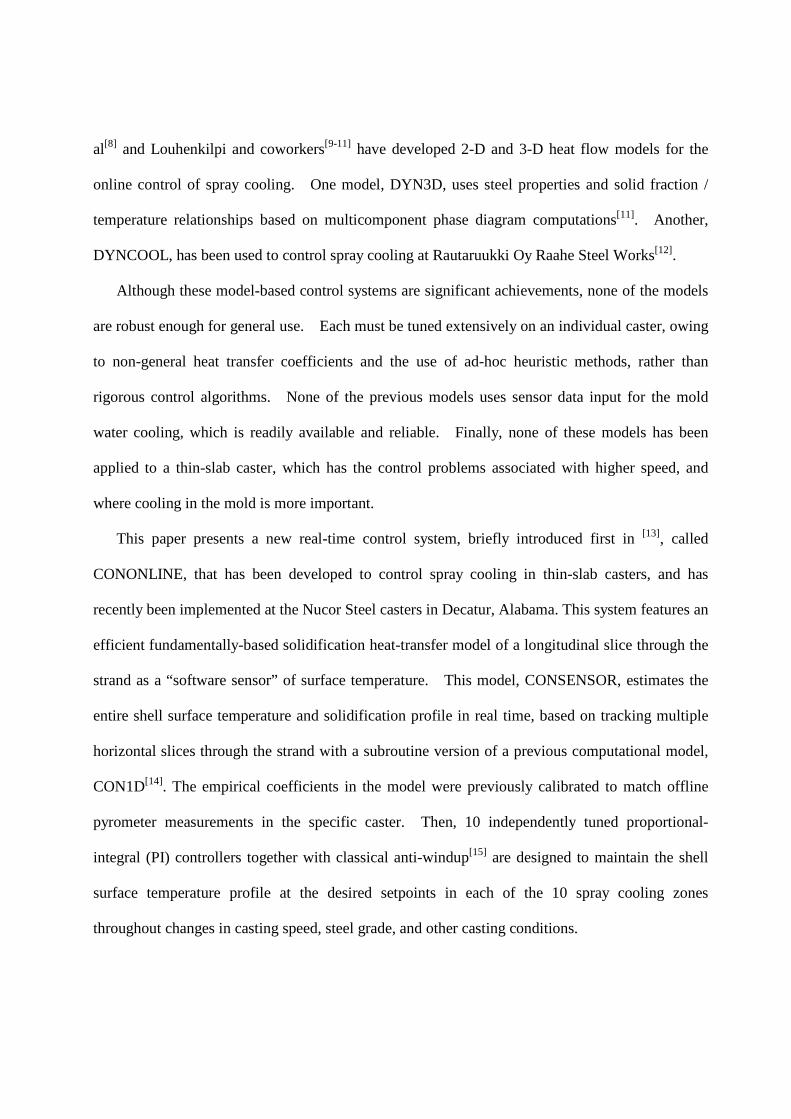
The new dynamic control system for thin-slab casters is based on the control diagram shown in
Fig. 1. The core of the system is a software sensor based on the CON1D heat-conduction model.
The software sensor, CONSENSOR, provides a real-time estimate/prediction of the strand state,
including the shell surface temperature distribution and metallurgical length. It updates based on
all the available casting conditions, which include: 1) conditions updated every second, such as

mold heat flux, casting speed, spray flow rates, strand width, etc; 2) heat-specific conditions such
as steel composition which are updated for heat changes during ladle exchanges; and 3) conditions
updated only when the software sensor is calibrated, such as roll and spray nozzle configuration,
heat transfer coefficients, etc. The estimated shell temperature profile is then compared against a
pre-determined surface-temperature profile setpoint, which also varies with casting conditions
such as mold heat flux, as described later. The mismatch between the estimate and the setpoint,
i.e. the tracking error, is then sent to a dynamic controller to compute the water flow rate command
required to drive the mismatch to zero. Finally, the computed command set of spray-water flow
rates is sent to the spray zone actuators in the operating caster (Level 1 control system), to the
Monitor program for visual display to caster operator, and also to the software sensor for
estimation at the next second.
Human-Machine Interface
Shell thickness and surface temperature estimation
Spray water flow rates
Setpointoptions
Software Sensor2-D transient thermal model
(200 moving 1-D slices)
steelsteel P steel
T TC k
t x xρ ∗ ∂ ∂ ∂ = ∂ ∂ ∂
ControllerSeparate PID controller for each spray zone
caster data
ΣΣΣΣ+
-
Caster
AUTOMATIC CONTROL LOOP
MAN/MACHINE SUPERVISORY
LOOP
SetpointGenerator
Surface temperature setpoint
pK
iK1
s
ΣΣΣΣ
ΣΣΣΣ
Saturation
ΣΣΣΣ +-
Figure 1. Software sensor based control diagram
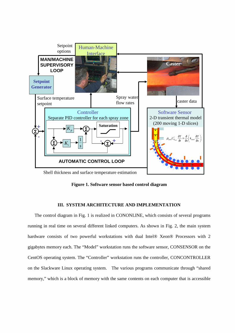
III. SYSTEM ARCHITECTURE AND IMPLEMENTATION
The control diagram in Fig. 1 is realized in CONONLINE, which consists of several programs
running in real time on several different linked computers. As shown in Fig. 2, the main system
hardware consists of two powerful workstations with dual Intel® Xeon® Processors with 2
gigabytes memory each. The “Model” workstation runs the software sensor, CONSENSOR on the
CentOS operating system. The “Controller” workstation runs the controller, CONCONTROLLER
on the Slackware Linux operating system. The various programs communicate through “shared
memory,” which is a block of memory with the same contents on each computer that is accessible
by any program and is updated continuously via TCP/IP CommServer and CommClient. A
separate TCP server C program (ActiveXServer) transmits the information to up to 16 Windows
PCs running a human-interface Visual C++ Monitor program. The Monitor program displays the
results and accepts user input while running simultaneously on several different computer screens.
The CONSENSOR model is a FORTRAN program, owing to its computational efficiency.
These programs are listed in Table I.
Controller Computer
(Slackware Linux)
CommServer
shared memory
CommServer
CONCONTROLLER
ActiveXServer Model Computer
(CentOS Linux)
shared memory
CommClientCONSENSOR
Windows Computers
CononlineMonitor
CononlineMonitor
TCP/IP connection
Shared memory connection
Legend:
Molten Steel
z
Meniscus
Slab
Torch Cutoff Point
Tundish
Mold
Ladle
Support Roll
Strand
Liquid Pool Metallurgical
Length
Spray Cooling Solidifying Shell
Submerged Entry Nozzle
Caster Automation
CommClient
Current control logic
Figure 2. Software sensor based control system architecture

Program Name Function
CONSENSOR estimating/predicting the profile of shell temperature and
thickness based on CON1D
CONCONTROLLER computing the required spray water flow rate to maintain
temperature setpoint
CONONLINE
Monitor
displaying in real-time shell surface temperature, thickness
profile estimates/predictions, computed water flow rate
and casting conditions
TCP/IP server working with TCP/IP client programs to transfer data
between workstations
TCP/IP client working with TCP/IP server programs to transfer data
between workstations
ActiveXServer TCP server working with monitor programs to transfer
data between controller workstation and PCs running
CONONLINE Monitor
Table I. Software programs in the control system
The control system in Fig. 2 has two operation modes: 1) shadow mode, which displays the
caster status and model predictions, and 2) control mode, which also controls the caster, when it is
switched on in the level 2 system. Shadow mode allows the control system to be tested and tuned
using real caster data, while the old controller controls the secondary cooling in the actual caster.
During shadow mode operation, many causes of crashes and errors were identified and solved,
with the help of checks to ensure that input data stays within reasonable bounds. The system is
now very robust and maintains stable operation through any set of conditions, including serious
disruptions or errors in input data. This operating mode also enables operators to make system
changes according to their experienced interpretation of the software sensor predictions. With
the benefit of shadow mode displaying the changing position of the metallurgical length, operators
at Nucor, Decatur ran the north caster with no incident, while the south caster, which did not have
CONONLINE, experienced a whale defect.
In either mode, the level 2 system sends the casting conditions such as casting speed, mold
heat flux, etc. at each second to the Controller workstation via the TCP/IP client. The casting
conditions are received by the TCP/IP server in the Controller workstation and relayed to the
Model workstation via its client. These data are available immediately to the sensor and controller
via the shared memory in each workstation. The software sensor then estimates the shell
temperature distribution in ~0.5s. The controller reads this distribution from shared memory and
computes the spray-water flow rates to maintain the selected setpoints, every 1s. To ensure
timely updating, data in each shared memory are exchanged ~10 times per second with
transmissions <20 ms each.
The predicted shell surface temperature and shell thickness profiles are transmitted via TCP/IP
to up to 16 Monitor programs, to be displayed on the operator console and elsewhere in real time.
The Monitor program is updated every 3s, which is slower than the 1s controller updates in order
to lessen transmission traffic on the steel mill general network. In control mode, the spray-water
flow-rate commands are also sent to the level 2 system to be applied in the level 1 system flow
actuators in the actual caster. Finally, changes to the temperature setpoints or control mode
requested by the operator through the monitor are sent to the other computers, in preparation for
the next time increment.
IV. SYSTEM COMPONENTS
A Heat Transfer Model - CON1D
CON1D is a simple but comprehensive fundamentally-based model of heat transfer and
solidification of the continuous casting of steel slabs, including phenomena in both the mold and
the spray regions[14]. The accuracy of this model in predicting heat transfer with solidification has
been demonstrated previously through comparison with analytical solutions of plate solidification
and plant measurements[14, 16]. Because of its accuracy, CON1D has been used by the steel
industry to predict the effects of changes in casting conditions on solidification and to develop
practices to prevent problems such as whale formation[17].
The simulation domain in this work is a transverse slice through the strand thickness that spans
from the shell surface at the inner radius to the outer radius surface. The CON1D model computes
the complete temperature distribution within the solid, mushy, and liquid portions of the slice as it
traverses the path from the meniscus down through the spray zones to the end of the caster at torch
cutoff. CON1D solves the following 1-D transient heat conduction equation within the
solidifying steel shell, using an explicit central finite-difference algorithm:
22
*2
( , ) ( , ) ( , ) i i steel i
steel steel steel
T x t T x t k T x tCp k
t x T x
∂ ∂ ∂ρ∂ ∂ ∂
∂ = + ∂ (1)
where ksteel is thermal conductivy, ρsteel is density, and *steelCp is the effective specific heat of the
steel, which includes the latent heat. In order to produce an estimate for the entire caster, the
software sensor uses multiple simultaneous runs of CON1D, hence the subscript i indicates the
temperature history of a particular slice.
This Lagrangian formulation takes advantage of the high Peclet number of the continuous
casting process, which renders axial heat conduction negligible[14]. The effect of non-uniform
distribution of superheat is incorporated using the results from previous 3-D turbulent fluid flow
calculations within the liquid pool[14]. Thermal properties vary with temperature according to
composition-dependent phase fractions. Microsegregation effects are included via a modified
Clyne-Kurz model[14, 18]. Shell thickness is defined by a liquid fraction of 0.3. The latent heat
of solidification is incorporated using an efficient enthalpy method and a post-time-step
correction[14]. Good accuracy is achieved using a grid spacing of approximately 1 mm and finite-
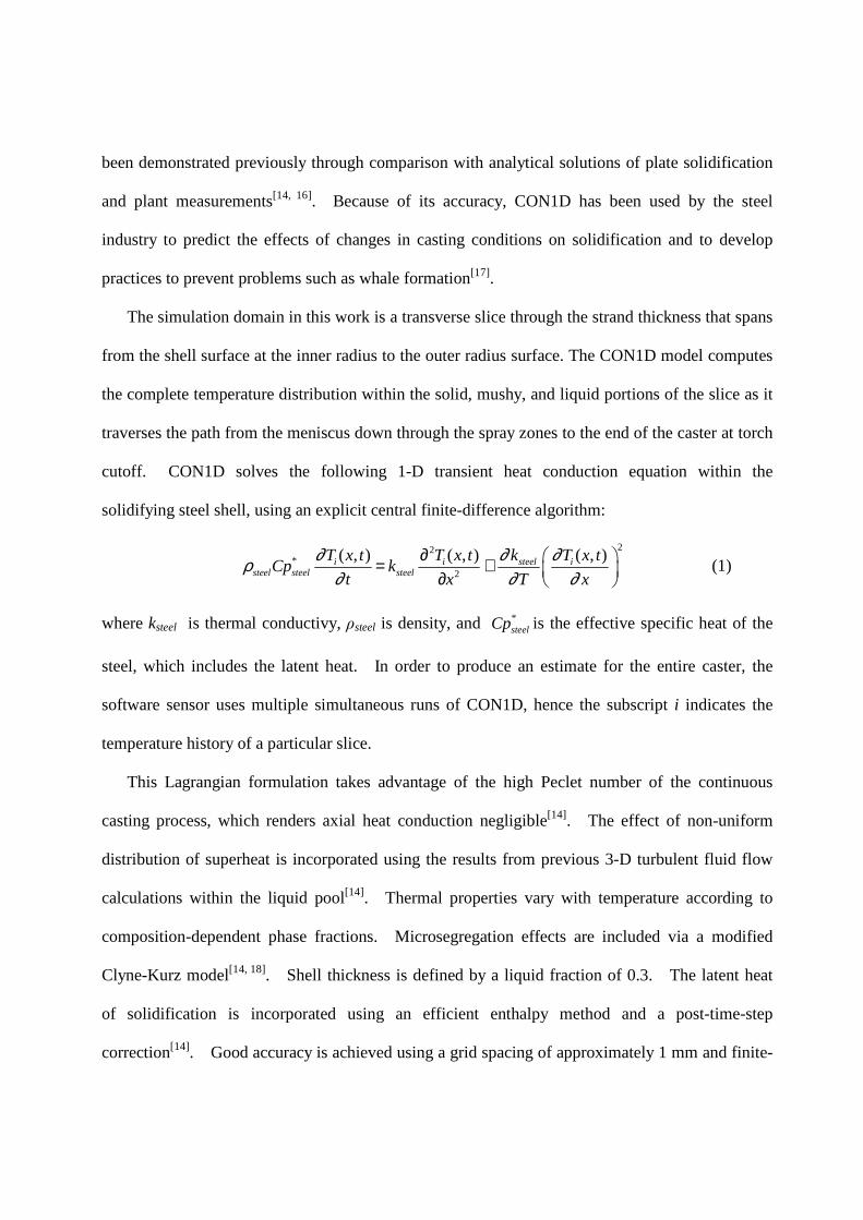
difference time-stepping size of 0.03s. With this tool used as a subroutine by the software sensor,
CONSENSOR, the closerd-loop diagram of Fig. 1 takes the form shown in Fig. 3. The model
box contains the explicit discretized form of Eq. (1) solved by CON1D [14]. Initial condition
(I.C.) is the pour temperature, measured in the tundish, and B.C. boundary conditions (B.C.) are
summarized below, with further detail provided elsewhere [14].
CONSENSOR
CasterSetpoint
generation
Average overspray zone
P Pj j ju k T= ∆
Σ
Σ
Setpointinterpolation
, , , ,mold c pour spray pattern sprayq V T n T
Σ
{ }, , 1, , , , ,
zoneN
m caster j j roll j roll j jz d l w n d
=
{ }xp
,I I prev Ij j j ju u k T t= + ∆ ∆
{ }1
zoneN
j ju
=′
sT
T̂
CONCONTROLLER
T
Σ
Zone-based control calculation
{ }1
zoneN
j ju
=
Delay interpolationbetween slices
( ) ( )
( )
2
1 1 1 12 2
1 1 2 12
_ _2
4
2 _ _
new steel steeli i i i i i i
steel psteel steel psteel
new new steel steelsurf
steel psteel steel psteel s
t step k kt stepT T T T T T T
x C x C T
t step k kt step qT T T T T
x C C T k
ρ ρ
ρ ρ
− + + −∗ ∗
∗ ∗
∆ ⋅ ∂∆= + − + + −∆ ⋅ ⋅ ∆ ⋅ ⋅ ∂
⋅∆ ⋅ ∂∆= = + − +∆ ⋅ ⋅ ⋅ ∂
BC: 2
2 _
teel steel psteel
t step q
x Cρ ∗
∆ ⋅− ∆ ⋅ ⋅
CON1D (slice model)
Mold region
mold
0
mold m
pourz
q q t
T T=
= ⋅
=
∫BC:
IC:
( ) ( )( )
_
0,me
sprays spray rad spray conv conv amb
i i mz z
q h h h h T T
T T x t t=
= + + + −
= +
BC:
IC:
Spray region( )0,i i mT x t t+
moldq
Mold cooling water
Strand in spray zoneStrand in mold
Spray cooling water
computed offline
Human-machine interface
Legendmeasurable outputs
unmeasureable outputs
inferred measurements
predicted state
manipulable inputs
internal signals
Figure 3. Closed-loop diagram with CONSENSOR estimator/predictor and CONCONTROLLER control algorithm
1. Boundary conditions in the mold
A new method has been developed to accurately define the surface heat flux profile in the
mold. In previous work, the CON1D model computes the surface heat flux within the mold
region by solving a two-dimensional heat equation in the mold and several mass and heat balance
equations within the interfacial gap[14, 19]. Its accuracy to predict mold heat transfer has been
verified against a full three-dimensional finite element analysis, as well as plant measurements[16].

13
For the present model, the average heat flux in the mold is found from the measured
temperature rise and flow rate of the cooling water, which is supplied through the level 2 system in
real time. The surface heat flux profile down the mold, qmold (MW/m2), is fit with the following
empirical function of time to match the average measured mold heat flux, q mold (MW/m2). This
function is split into a linear portion and an exponential portion:
( ) ( )( )
( )
0 00
0 0
, 0,
,
a i i ci
steel mold n
b i c i m
q q t t t t tT L tk q t
x q t t t t t t−
− ⋅ − ≤ − <∂ ± − = = ∂ ⋅ − < − ≤
(2)
where 0it is the start time for the slice and hence (t - 0
it ) is the time below meniscus, and n is a
fitting parameter that controls the shape of the curve, chosen to be 0.4. The initial heat flux, q0, is
the maximum heat flux at the meniscus, chosen to be:
0 mold facq q q= ⋅ (3)
where qfac is another parameter, set to 2.3. The total time spent in the mold, tm, is calculated by
c
mm V
zt =
(4)
where zm is the mold length and Vc is the casting speed. The duration of the linear portion, tc, is
assumed to be
facmc ttt ⋅= (5)
where tfac is a third parameter, set to 0.07. Then the intermediate parameters qa and qb are defined
below, based on keeping the curve continuous, and matching the total mold heat flux in the mold
with the area beneath the curve.
( ) ( ) ( )
( )
1
0 0
1 1 2
11
12
n n
c m mold m ca
n nc m c
q t t n q t n q tq
t t n t
−
+ −
⋅ − − ⋅ ⋅ − ⋅ ⋅=
⋅ − + (6)

14
( ) ( ) 10
+−⋅= nca
ncb tqtqq (7)
Fig. 4 compares heat flux profiles predicted with this new model to previous measurements in
thin-slab casting molds[16, 20].
0
1
2
3
4
5
6
7
8
9
0 100 200 300 400 500 600 700 800 900 1000
Distance Below Mensicus (mm)
Hea
t F
lux
(MW
/m2)
Park heat flux [2.84 MW/m2]
Park heat flux (CONONLINE)
Santillana heat flux [2.63 MW/m2]
Santillana heat flux (CONONLINE)
Figure 4. Comparison of CONONLINE mold heat flux profiles from Eqs. (2)-(7) with
measurements from [16] and [20].
2. Spray-zone boundary conditions
Below the mold, heat flux from the strand surface is given by
( ) ( )( ),,i
steel i amb
T L tk h T L t T
x
∂ ±− = ± −
∂ (8)

15
where Tamb is the ambient temperature and h (W/m2K) varies greatly between each pair of support
rolls according to components: spray nozzle cooling (based on water flux), hspray, radiation,
hrad_spray, natural convection, hconv, and heat conduction to the rolls, hroll, as shown in Fig. 5.
Incorporating these phenomena enables the model to simulate heat transfer during the entire
continuous casting process. Spray cooling heat extraction is specified as the following function
of water flow rate[1] :
( ), 1cspray sw j sprayh A Q b T= ⋅ ⋅ − ⋅ (9)
where Qsw,j (L/m2s, where L stands for liters) is water flux in spray zone j and Tspray is the
temperature of the spray cooling water (°C). For air-mist nozzles, this work assumes that air flows
are consistent functions of water flow, so are not considered separately.

16
Surface Temperature (°°°°C)
Dis
tan
ce (
mm
)
1000 1100 1200 1400
1
300
1
200
1
100
Slab
Roll
Spray nozzle
natural/forced convection, hconv
radiation, hrad
spray impinging, hspray
roll contact, hroll
Heat Transfer Coefficient
Figure 5. Schematic of spray zone region
Finding parameters to accurately predict spray cooling heat extraction presents a significant
challenge that has been the focus of several previous experimental studies. In Nozaki’s empirical
correlation[21], A = 0.3925, c = 0.55, b = 0.0075, which has been used successfully by other
modelers[1, 21, 22]. Others describe the variation of heat flux with nozzle type, nozzle-to-nozzle
spacing, spray-water flow rate, and distance of the spray nozzles from the strand surface, based on
plant and lab studies[1, 23, 24]. Recent experimental work aims to develop more fundamental heat
transfer relationships for spray cooling, based on droplet size and impact[25, 26], including studies of
air mist cooling[26, 27]. This work combines previous correlations with recent lab measurements
of the spray patterns obtained from the nozzles used in the caster of interest in this work[28, 29].

17
To further improve fundamental prediction of spray-zone heat extraction, experimental
measurements using a new steady-state apparatus are being conducted[30]. The well-known drop
in heat extraction from the sprays on the bottom surface of the strand, and the increase in heat
extraction due to the Leidenfrost effect at lower temperatures, both can be accommodated, but
await these measurements.
Radiation, hrad_spray is calculated by:
( )( )2 2_ , ,rad spray steel i s K ambK i s K ambKh T T T Tσ ε= ⋅ + + (10)
where Ti,sK is the surface temperature of the strand, Ti(±L,t), expressed in Kelvin, σ is the Stefan-
Boltzman constant (5.67 x 10⁻⁸ W/m2K4), and εsteel is the emissivity of the strand surface, 0.8, and
TambK is ambient temperature, 298 K. Natural convection is not important, so is treated here as a
constant 8.7W/m2K. The heat transfer coefficient extracting heat into each roll, hroll, is expressed
as a fraction of the total heat extracted to the rolls, froll, which is calibrated for each spray zone:
( ) ( ) ( )( )
_ _
1rad spray conv spray spray rad spray conv spray pitch spray roll contact
roll rollroll contact roll
h h h L h h L L Lh f
L f
+ + ⋅ + + ⋅ − −= ⋅
⋅ − (11)
This fraction can be based on the measured water temperature increase of roll cooling water,
augmented with some external sprays. Increasing froll increases the severity of local temperature
drops beneath the rolls. Severity also depends on the length of the roll contact region, Lrollcontact,
based here on assuming a contact angle with the roll of 10°. Beyond the spray zones, heat
transfer simplifies to radiation and natural convection.
3. Model Calibration and Example Results
CON1D has been validated with plant measurements in the spray zones on several different
operating slab casters [14, 16, 31]. This versatile modeling tool has been applied to a wide range of
practical problems in continuous casters. For the current work, the model was further calibrated
18
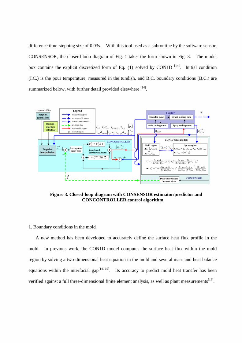
to match the average surface temperatures measured under steady-state conditions using five
Modline® 5 pyrometers installed along the south Nucor caster in Decatur, Alabama in January,
2006. Each pyrometer was centered between two neighboring rolls and between spray nozzles
with an approximate stand-off distance of 203 mm from the strand surface, as shown in Fig. 6.
They were located 3866mm, 6015mm, 8380mm, 11385mm and 13970mm, from the meniscus.
Temperature was converted using linear transformation of the voltage signal and averaged over
450 seconds. Each measurement was estimated to average over a 15mm diameter spot.
Figure 6. Pyrometer arrangement in the south Nucor caster

19
A typical example of the steady state experiments is given here to demonstrate the calibration.
A 90mm thick x 1396mm wide thin slab of low carbon steel (0.24%C, 1.09%Mn, 0.0019%S,
0.014%P, 0.175%Si, 0.04%Cr, 0.04%Ni, 0.087%Cu, 0.01%Mo, 0.002%Ti, 0.039%Al, 0.001%V,
0.0076%N, 0.035%Nb) was cast at 3.61 m/min. Pour temperature was 1547.8oC, and average
mold heat removal was 2.4243 MW/m2. Average flow rates are shown in Table II. Other
conditions and details on the roll and caster dimensions are given in Tables II and elsewhere[32].
The average pyrometer temperatures with error bars to indicate the standard deviation are shown in
Fig. 7 a) together with the strand outer surface temperature profile predicted by CON1D. The
dips in temperature profile are caused by roll contact and spray cooling, whereas the temperature
peaks occur where convection and radiation are the only mechanisms of heat extraction. Dips
and peaks are shown clearly in Fig. 7 b) for a zoom-in on a roll spacing. Local temperature drops
beneath the rolls of slightly over 100oC are produced from a typical froll value of 0.36. Local drops
beneath each spray-nozzle impingement region vary from 30-80 oC according to spray zone
conditions.
Spray zone
# of rolls
Roll radius (m)
Roll pitch(m)
Spray length(m)
Spray width(m)
froll Qsw (L/min/roll)
1 1 0.062 0.090 0.05 1.640 0.01 79.8 2 5 0.062 0.165 0.05 0.987 0.08 188.0 3 6 0.062 0.177 0.05 0.987 0.22 123.0 4 5 0.070 0.189 0.05 1.008 0.20 50.6 5 10 0.080 0.213 0.05 1.620 0.36 50.6 6 10 0.095 0.236 0.05 1.680 0.36 26.0 7 12 0.095 0.249 0.05 1.680 0.36 47.4
Table II. Spray zone input values for CON1D simulation of experimental case conditions

20
a) along entire domain b) close-up near one roll spacing
Figure 7. Shell surface temperature comparison of CON1D predictions and pyrometer measurements
The shell thickness predicted by the model (based on the solid fraction of 0.7) is also shown in
Fig. 7 a). Note that the entire cross-section is solid just prior to exit from the roll support region,
which is consistent with plant experience for these conditions. The predicted temperatures
generally exceed those measured by the pyrometers, except for the last pyrometer, which is outside
the spray chamber and expected to be most reliable. The difference is believed to be due to the
pyrometers reading lower than the real temperature, owing to steam-layer absorption and surface
emissivity problems. Further calibration work is needed to improve the accuracy of the
pyrometer measurements, the spray heat-transfer coefficients, the spray-zone lengths, and the
predicted variations in surface heat transfer and temperature, in order to improve the agreement.
B Software sensor - CONSENSOR
The function of the software sensor is to accurately predict the temperature distribution in the
strand in real time. The program CONSENSOR was developed to produce the temperature

21
profile along the entire caster (z) and through its thickness (x) in real time (t), by exploiting
CON1D as a subroutine. It does this by managing the simulation of N different CON1D slices,
each starting at the meniscus at a different time to achieve a fixed z-distance spacing between the
slices. This is illustrated in Fig. 8 using N = 10 slices for simplicity.
Boundary Actuation:Cooling water spray rate, u(t), generates heat flux hspray(Ti(±L ,t – Tamb)
Boundary Sensing:• Mold heat removal rate, Qmold(t)• Boundary point temperature
measurements from pyrometers, Ti(±L ,t)
Boundary Disturbances:Uncontrolled heat flux from: roll/shell contact points, radiation, natural convection, (hroll + hrad_spray+ hconv)(Ti(±L ,t) – Tamb)
Model:1D slices traversing 2D cross-section of 3D strand, Ti(x,t)
Control Objective:Temperature along shell surface,Ti(±L ,t)
Slice velocity, Vc
zx
Figure 8. CONSENSOR simulation domain
The control algorithm requires that CONSENSOR provide an updated surface temperature
estimate, T̂ (z,t), every ∆t seconds. Note that the coordinates for Ti in CON1D slices (distance
through thickness and time) are not the same as the coordinates for T̂ in CONSENSOR (distance

22
from meniscus and time). The surface temperature estimate T̂ is assembled from the slice
profile histories Ti, as follows.
During each time interval, the N different CON1D simulations track the evolution of
temperature in each slice over this interval, given the previously-calculated and stored temperature
distributions across the thickness of that slice at the start of the interval. The computation time
required is about the same as just one complete CON1D simulation of the entire caster length,
which takes about 0.6 seconds on the CentOS workstation when casting at 4.5 m/min.
During program startup, the simulation for slice i + 1 begins when slice i passes 75 mm from
the meniscus. After startup, a new slice begins immediately from the meniscus whenever a slice
reaches the end of the caster. Currently, CONSENSOR always manages exactly 200 slices,
which corresponds to a uniform spatial interval of 75mm along the caster length, zc, which is 15m.
The complete temperature history for each slice is stored from when it started at the meniscus, 0it ,
to the current time, t. To assemble the complete temperature profile needed each time interval
requires careful interpolation of the results of each slice at different times.
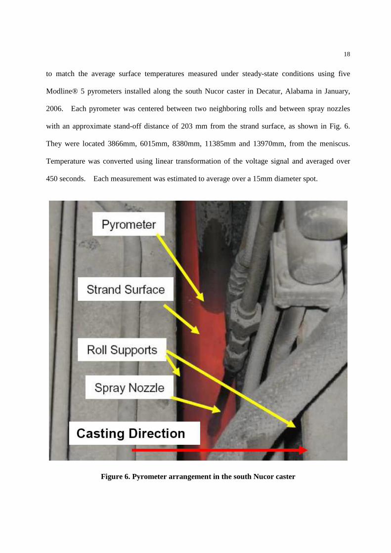
When plotted on a two-dimensional t-z grid, the desired output domain of the software sensor
is a horizontal line, as shown in Fig. 9. For instance, at time t* the sensor must predict ̂T (z,t*)
for the entire caster length, 0 ≤ z ≤ zc. However, the surface temperature included in a single slice
history from CON1D traverses a monotonic-increasing curve in the t-z plane. At constant casting
speed, Vc, these curves are straight diagonal lines with slope of 1/Vc. Fig. 9. shows two such lines
representing two slices created at times 01t and 0
2t . It is clear from Fig. 9 that each complete run
of CON1D contributes only one data point to the desired software sensor output at each time, e.g.
T̂ (zi(t*),t*), where zi(t) is the location of the ith slice at time t, which is calculated by
23
( ) 0, 1,2,..., 200
i
t
i ctz t V d iτ= =∫ . (12)
With constant casting speed, this integral simplifies to Vc(t – 0it ), (Fig. 9). Data points in the
temperature profile estimate such as T̂ (zi(t*),t*), which come directly from CON1D output, are
exact estimation points.
CONSENSOR output domain
CON1D ou
tput d
omain
Distance below meniscus, z
Tim
e, t
( )01 1, / cT x L t t z V= ± = +( )0
2 2, / cT x L t t z V= ± = +
( )ˆ ,T z t t∗=t∗
t t∗ − ∆ ( )ˆ ,T z t t t∗= − ∆
01t
02t
( ),z t∗ ∗
( )01, / cz t z V∗ ∗+
( )( )01 ,cV t t t∗ ∗⋅ −
CON1D slices
CONSENSOR updates
Delay interpolation
Exact estimate
Surface temperature output locations
Figure 9. Illustration of incremental runs of CON1D and shell surface temperature profile approximation using multiple slices with delay interpolation
Fig. 10 illustrates the error introduced by interpolating spatially between these exact points.
The 75 mm span between slices in this work can pass over the temperature dips and peaks caused
by the roll and spray spacing, resulting in errors of 100 °C or more. This problem is overcome by

24
“delay interpolation,” interpolating temporally between the latest temperature histories available
from each CON1D slice, described as follows and illustrated in Fig. 9 using N = 2 slices.
5 5.2 5.4 5.6 5.8 6960
980
1000
1020
1040
1060
1080
1100
1120
Distance from meniscus (m)
She
ll su
rfac
e te
mpe
ratu
re (o C
)
Actual temperature profileExact slice estimatesSpatial interpolation of slice estimates
Figure 10. Example of the actual temperature profile, the exact estimates and spatially interpolated temperature profile
For locations between the exact estimate points, the surface temperature is approximated at the
current time using the most recent available temperature at that location from the CON1D slice
histories. Applying this method everywhere along the caster, the control-oriented shell surface
temperature profile prediction ̂T (z,t) is obtained at any time t:

25
( )( ) 1ˆ( , ) , where ( ) ( )i i i iT z t T x L t t z z t z z t+= = ± = < ≤ (13)
where zi(t) is given in Eq. (12), and ti(z) is the time when the ith slice was the distance z from the
meniscus, which is the inverse of Eq. (12):
( ) 0
0
z
i ic
dt z t
V
ζ= + ∫ (14)
For constant casting speed, this simplifies to 0it + z/Vc.
Fig. 9 illustrates this process at time t*. Starting from the previous time, t* – ∆t, the exact
shell surface temperature estimates are known at the previous locations of the two slices. The
simulation restarts for each slice and continues for the desired time interval, ∆t, giving temporally-
exact estimates at two new locations at time t*. The point (z*,t*) lies in between the locations of
these exact estimates, so according to the delay interpolation scheme, the surface temperature at
this point is approximated by the surface temperature of slice 1 when it passed the distance z* from
the meniscus. Thus, the temperature T1(±L, 0it + z*/Vc) from the history of slice 1 is used to
estimate the surface temperature T̂ (z*,t*).
The approximation error introduced at location z* in Fig. 9 is the temperature change at this
location from time t1(z*) to t* + ∆t, which is a function of the extent of transient effects in the
laboratory frame, and slice spacing. It follows that slices should be evenly distributed to
minimize the approximation error, and that the magnitude of this error decays to zero during
steady operation. Even during times of extreme transients, this error is easily recognized by
operators from the jagged appearance of the temperature profile, as it jumps from locations with
the worst delays to the exact points. Note that the interpolation delay for the point (z*,t*) in Fig. 9
is greater than the time interval, i.e. t1(z*) < t* – ∆t. This case arises for some points when the
slices travel less than the slice spacing during the time interval. During operation, the distance

26
simulated during each time interval increases with casting speed, but is usually less than the
distance between slices. Specifically, the 75mm span in this work is achieved only for speeds of
4.5 m/min or more. At lower speeds, the points further along each jag in the casting direction are
most accurate, because they contain the most recent temperature estimates.
C Control algorithm - CONCONTROLLER
Because heat transfer between slices is negligible, decentralized single-input-single-output
(SISO) controllers, which have no inter-controller interaction, can be used to control the spray-
water flow rates to minimize the error between the CONSENSOR prediction and the setpoint
temperature profile. A single multi-input-multi-output (MIMO) controller is another option, but is
more complicated to design and implement and does not offer much better performance.
The temperature control problem can be regarded as a disturbance rejection problem, in which
the heat flux from the liquid core at the liquid/solid interface inside the strand can be treated
approximately as a constant disturbance and the control goal is to maintain shell surface
temperature under this disturbance. In light of this observation, the control law is simply chosen as
the standard Proportional-Integral (PI) control. Here, the integral part is necessary for maintaining
the surface temperature with no steady-state error under a constant setpoint and rejecting constant
disturbances. Derivative control, which is normally introduced to increase damping and stability
margin, is not used since the system itself is well damped, owing to the high thermal inertia of the
solidifying steel strand.
An important feature of the caster spray configuration is that the rows of individual spray
nozzles are grouped into Nzone spray zones according to nozzle location and control authority
(which depends on how nozzles are connected via headers and pipes to a given valve). Each

27
individual spray zone corresponds to an area where the spray water to the nozzles has a single inlet
valve. This means that all rows of nozzles in a zone have the same spray-water flow rate and
spray density profile. This configuration is shown in Fig. 11 and listed in Table III, where uj
refers to the jth spray zone[32]. High in the caster, where the strand is vertical, nozzles on the inner
and outer radii are part of the same spray zone, so must be given the same spray flow rate
command. For the caster in this work, this is the case for the first 4 spray regions. The lower 3
zones each have a separate zone and spray command for the inner and outer radius surfaces.
Therefore, a total of Nzone = 4 + 2x3 = 10 independent PI controllers are needed. The parameters of
each controller are tuned separately to meet the control performance in each zone, and are listed in
Table IV. These gains were chosen by assigning initial values based on the average total water
flow through each zone, and then tuning by hand. CONONLINE provides model-based control
only for the center-line zones. Based on these 10 control signals, the spray flow rates for other
zones across the strand width are prescribed as a function of slab width using separate logic.
Generally, the flow rates per unit area are kept constant across the width, except in zones
containing strand edges, where they are turned down slightly to lessen overcooling of the slab
corners.
Spray zone
Segment Side wj (m)
lj
(m) Lj
(m) Controller
1 Foot rolls Both 1.640 0.05 x 2 0.090 x 2 u1
2 Upper bender Both 0.987 0.25 x 2 0.827 x 2 u2 3 Lower bender Both 0.987 0.30 x 2 1.061 x 2 u3 4 Segment 1 Both 1.008 0.25 x 2 0.946 x 2 u4
Inner 1.620 0.50 2.130 u5 5 Segment 2/3 Outer 1.620 0.50 2.130 u6 Inner 1.680 0.50 2.356 u7 6 Segment 4/5 Outer 1.680 0.50 2.356 u8 Inner 1.680 0.60 2.986 u9 7 Segment 6/7 Outer 1.680 0.60 2.986 u10
Table III. Controller assignments[32]

28
mold
u1
u2
u3
u4
u5
u6
u7
u8
u9
u10
Figure 11. Center spray zones configuration
Controller kP kI
1 0.4 0.4
2 2.0 1.0
3 1.2 0.6
4 0.5 0.4
5-6 5.0 0.125
7-8 5.0 0.5
9-10 1.8 0.8
Table IV. Controller gains
In accordance with this spray area configuration, the control algorithm proceeds through the
following steps (see Fig. 3). At each time, t, the inner and outer radii shell surface temperature

29
profile estimate, T̂ (z,t), is obtained by the software sensor as the multi-slice temperature
calculation aggregated by means of the interpolation procedure illustrated in Fig. 9. The desired
shell surface-temperature profile setpoints are represented as Ts(z,t), and discussed in Section IV-F.
1. Calculate the average tracking error for each zone:
( )zone
ˆ( , ) ,
( ) , 1,..., ,
s
jj zone
j
T z t T z t dz
T t j nL
− ∆ = =
∫ (15)
where Lj denotes the total length of zone j. In the upper caster, where the
spray zones cover both sides of the strand, the integral is over both sides and
Lj is consequently twice the physical length of the strand in that zone.
2. Calculate the spray-water flow rate command for the next time interval, uj(t +
∆t), for each controller using the following PI control laws:
( ) ( ) ( )( ) , 1,..., ,P Ij j j j j j zoneu t t k T t u t k T t t j n + ∆ = ∆ + + ∆ ∆ = (16)
where the bracketed portion is a discrete-time integral over the time interval
∆t, (1s). The proportional and integral gains for each controller, Pjk and
Ijk respectively, are given in Table IV.
Note that (16) is a recursive definition, and so the initial settling time of the PI controller will
depend on the initial choice of the control output, uj(0), supplied when the control algorithm
begins its calculations. During casting startup, PI control starts in a given zone only after steel
has entirely filled the zone. Before this time, control is chosen based on the spray–table control
method described in Section IV-F. When the PI control calculation begins for zone j, the spray-
30
water flow rate from the spray-table is assumed as an initial value of uj to reduce the initial settling
time.
The control command uj(t), which is the requested water flow rate to spray zone j in L/s, is sent
to the caster automation Level 1 control system. The flow rate through the valve governing spray
zone j, uj′(t), is measured by the caster automation and sent to CONSENSOR in order to estimate
the surface heat flux using Eq. (9). The spray-water flux used in Eq. (9) is currently assumed
uniform over the nozzle footprints in each zone, and is calculated by:
( ) ( ),
jsw j
j j
u tQ t
l w
′= (17)
where Qsw,j is the spray-water flux from each row of nozzles in zone j, wj is the width and l j the
total length of the area of the steel surface upon which all the sprays in zone j impinge. The
dimensions (Table III) differ between spray zones according to how the distribution headers are
constructed.
Finally, classical anti-windup[15] is adopted to avoid integrator windup when the transient
control commands fall outside the range of feasible spray rates. Due to the physical limitations of
the spray cooling system at the caster, it is common that the instantaneous spray rate requested by
the control logic, uj(t), exceeds the maximum or is less than the minimum limit achievable by the
nozzles, so the measured spray rate, uj′(t), is different. The requested and measured spray rates
may also be different due to dynamics such as actuator interactions with the header piping system.
These differences tend to cause controller instability, known as “windup”. This problem is
prevented by subtracting the difference from the integral portion of the control command, uj′(t):
( ) ( ) ( ) ( ) ( )( ) ,I I I awj j j j j j ju t t u t k T t t k u t u t′+ ∆ = + ∆ ∆ − − (18)

31
where awjk is a tuning parameter which can be used to relax the rate of windup. Here, these
parameters are set to 1. The computational closed-loop diagram Fig. 3 shows this antiwindup
scheme graphically.
D Combining CONSENSOR and CONCONTROLLER – Certainty Equivalence and Loop Closure
Issues
The PID bank in the CONCONTROLLER system developed here uses strand surface
temperature in the secondary cooling region estimated by an observer (CONSENSOR model
program) to define its output error: deviation from the desired temperature-profile setpoints. In
control terminology, this is the "certainty equivalence principle" – using the estimate as if it were
the true value.
The loop closure employed here, however, has some special features. In the mold,
CONSENSOR performs closed-loop estimation, with the temperature estimate being quite
accurate, because it is based on the measured mold heat removal rate and an accurate boundary
heat flux profile (cf. Section IV-A-1 and Fig. 3). The estimated slice temperature profile at mold
exit, denoted Ti(x, 0it + tm) in Fig. 3, is referred to as an inferred measurement[33] because it is
produced by a model from a secondary measurement. Due to the temperature continuity at mold
exit, this inferred measurement becomes the initial condition for the slice prediction in the
secondary cooling region. Hence, at the start of the secondary cooling region, the control system
achieves inferential closed-loop control.
In the rest of the secondary cooling region, reliable real-time heat-transfer measurements are
not possible, so the controller uses open-loop model-based temperature estimates. The quality of
these estimates is still very good because in addition to being accurately initialized at mold exit,
32
the model correctly incorporates the effects of several casting process changes (casting speed,
superheat, grade, etc.) on strand-temperature evolution from a fundamental basis and has been
calibrated offline to correctly predict whale formation under a few typical conditions. However,
several other process variations, such as hysteresis in the boiling heat transfer coefficients and
spray-nozzle clogging, are not modeled in CONSENSOR. Without the ability to measure the
strand surface temperature accurately and robustly in real time, surface temperature estimate
accuracy could deteriorate with distance below mold exit.
This combination of closed-loop estimation localized at mold exit (i.e. spatially discrete) with
open-loop estimation throughout the rest of the strand (i.e. spatially continuous) is strictly termed a
hybrid discrete-continuous[34] closed-loop/open-loop observation of the strand temperature profile
in the secondary cooling region. The resulting control system can thus be termed hybrid closed-
loop/open-loop system, as well. Even if the placement of reliable pyrometers becomes
technically feasible in the future, the pyrometer measurements are still essentially spatially discrete
and strand temperature in the gaps between pyrometers would have to be estimated in the open
loop. Hence, the control system would retain this hybrid nature. Since this reinforces the
importance of modeling accuracy to ensuring estimator quality, lab measurement of heat transfer
coefficients during air-mist spray cooling and further calibration with plant measurements is being
addressed as another important aspect of the larger project.
E Visualization - Monitor
Although not an element of the control diagram in Fig. 1, the monitor is an important
component in the control system because it provides real-time display of many variables, setpoints,
and results, permitting operators and plant metallurgists to monitor the caster and the control
33
system performance and to make adjustments as needed. In addition to the instantaneous casting
conditions, the monitor displays for both the outer and inner radii: the estimated shell surface
temperature profiles, the corresponding temperature setpoints in each zone, estimated shell
thickness growth profile, controller-requested water flow rates control commands in each zone, the
corresponding measured flow rates, and other parameters. To avoid network traffic problems, the
refresh rate on the Monitor is 3 seconds.
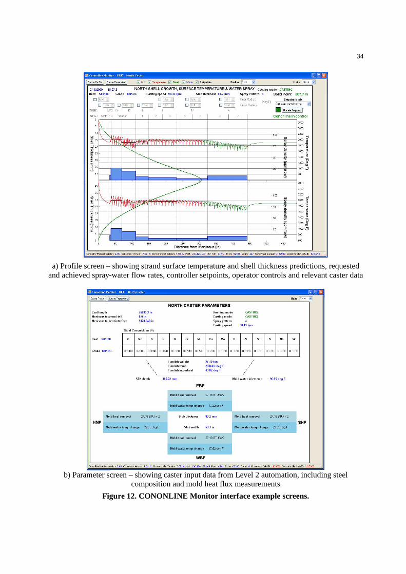
Fig. 12 shows typical screen shots of both monitor interface windows. Fig. 12a shows the
“profile screen.” This screen serves two purposes. The first purpose is to relay key simulation
outputs to the operators and plant engineers. Important caster parameters such as casting speed
and final solidification point are noted at the top of the screen. The two opposing shell profiles
form a V-shape that looks like the real liquid pool. Together with the superimposed temperature
profiles, it is easy to visualize the state of the caster. The second purpose of the profile screen is
to supply an interface for operator input to the controller, via a drop-down box of setpoint
generation options, and individual controls to change the temperature setpoint in any zone
manually. The controller can generate temperature setpoints in several ways, as described in the
next section. Fig. 12b shows the “parameter screen,” which displays the most important caster
measurements input to the model. This allows for easy checking of the casting conditions, and
TCP/IP server and client operation.
34
a) Profile screen – showing strand surface temperature and shell thickness predictions, requested and achieved spray-water flow rates, controller setpoints, operator controls and relevant caster data
b) Parameter screen – showing caster input data from Level 2 automation, including steel
composition and mold heat flux measurements
Figure 12. CONONLINE Monitor interface example screens.

35
The importance of the monitor as part of the control system should not be underestimated.
By presenting accurate information to the operator in real time in a natural visual manner, this
system empowers the operator to react better to unforeseen situations. In addition to controlling
surface temperature, another important objective of the system is to avoid costly and dangerous
“whale” formation. A whale forms when the metallurgical length extends past the last set of
support rolls, and the internal ferrostatic pressure causes excessive bulging of the strand. While
this system was being tested at Nucor Decatur on the North Caster, prior to giving it full automatic
control, operators watching the monitor were able to recognize impending problems and avoided
whale formation. The South Caster, which did not have the system, experienced a whale during
this time. Ultimately, a truly “expert” caster control system should recognize and take
appropriate action to prevent these and other problems, in addition to controlling sprays to
maintain surface temperature.
F Setpoint Generation
Choosing good setpoints for spray cooling is as challenging and important as the control task
itself. Several different methodologies are explored in this work. The current (old controller)
spray practice is based on “spray-table control.” The spray flow rates in each zone down the
caster, or “spray pattern” that produces good quality steel for a specific group of steel grades in a
specific caster are determined from plant trial and error and previous experience. Higher casting
speed requires higher water flow rates to maintain the same cooling conditions (see Table V for
typical spray practices used in this work). Thus, for each spray pattern, a different spray profile is
tabulated for each casting speed in a grid (database) that spans the range of normal operation.

36
During casting, spray setpoints are interpolated from the appropriate spray-table database for the
chosen pattern, according to the current casting speed. This method has the disadvantage that it
does not accommodate transient behavior in the strand.
Table V. Nominal spray fluxes in simulations
Previous theoretical knowledge on optimizing spray cooling is defined in terms of steady-state
surface-temperature profiles to avoid various embrittlement and cracking problems that are
associated with particular temperature ranges[2]. Furthermore, surface temperature variations
with time, such as occur during speed changes, startup, and tailout, are detrimental because they
cause surface stress and defects. To combine these two types of knowledge, the spray tables were
converted to tables of surface temperature profile setpoints. As shown in Fig. 3, this is a two-step
process comprised of the generation of setpoint profiles offline, and the interpolation of these
profiles during casting. To generate the setpoints, CON1D was run for every casting speed and
all patterns according to the tabulated spray profiles. The resulting temperatures are stored in a
two-dimensional array (according to speed and pattern). During operation, these profiles are
interpolated to find the desired temperature profile for the current casting speed and pattern to use
Controller Qsw at 3.0 m/min
(L/s/m2)
Qsw at 2.5 m/min
(L/s/m2)
u1 13.46 11.54
u2 40.15 30.44
u3 31.97 22.81
u4 11.89 6.27
u5 5.61 1.80
u6 5.61 1.80
u7 3.23 1.05
u8 4.81 1.66
u9 10.24 10.24
u10 10.24 10.24

37
as the setpoint for the PI controller, Ts(z,t). This second approach is referred to as “speed-
dependent temperature setpoints”.
However, the temperature setpoints need not vary with casting speed during operation. If the
computational model is reliable, it is better to use a constant temperature setpoint for all casting
speeds. In this work, a representative profile was chosen from each pattern in the speed-
dependent temperature-setpoint database, reducing the setpoint table by one dimension. This
approach takes advantage of the fact that steel thermal properties are relatively independent of
steel grade and casting speed, so that quality depends mainly on surface temperature profile.
During offline (shadow mode) plant testing, the controller output using fixed temperature
setpoints called for many sharp changes in spray rate in the first few spray zones. It was
discovered that this was caused by significant variations in strand surface temperature at mold exit
with changes in mold heat flux, casting speed, and steel grade. Forcing the surface temperature
to change quickly to a specified temperature setpoint causes detrimental sharp changes in shell
surface temperature, especially in the first two spray zones below the mold. Such changes, and the
associated thermal stresses, are what setpoint-based control is supposed to avoid.
The root of the problem is that temperature profiles are sensitive to the mold heat flux, which
is not accounted for in the spray table. To generate the setpoints, the average mold heat flux
needed for Eq. (3), q mold was estimated as a function of mold powder and casting speed, from the
following empirical correlation[35]:
26 0.09 1.19 0.47
0
0.107 %4.63 10 1 0.152exp
0.027mold flow c
Cq T Vµ − −
− = ⋅ − −
(19)

38
where: q mold0 is the estimated average mold heat flux (MW/m2), µ is the powder viscosity at
1300º C, (Pa-s), Tflow is the melting temperature of the mold flux (ºC), Vc is the casting speed
(m/min), and %C is the carbon content (pct).
Even though this equation reasonably predicts mold heat flux at the caster in this work, (and
could be tuned to be even better), the effects of unaccounted variables (such as mold powder
changes, superheat effects, and random variations) always cause the measured mold heat flux, and
the corresponding surface temperature at mold exit to change significantly with time at a given
casting speed (setpoint).
To avoid this problem, a new setpoint strategy, called “fixed temperature setpoints” was
developed that allows the temperature profile setpoints to vary with mold heat flux, and
consequently with mold exit temperature. Five different temperature profile setpoint curves are
generated using CON1D with 0.7q mold0, 0.85q mold0, q mold0, 1.15q mold0, and 1.3q mold0. An
example of the 5 temperature setpoint curves for one particular pattern is shown in Fig. 13. It can
be seen that these setpoints produce mold exit temperatures that span a wide range from 850 to
1250 °C. This third strategy again stores a two-dimensional array of fixed temperature setpoints
(organized according to mold heat flux and pattern).

39
0 5 10 15700
800
900
1000
1100
1200
1300
1400
1500
1600
Distance from meniscus (m)
Tem
per
atur
e (o C
)
1.66 MW/m2
2.01 MW/m2
2.37 MW/m2
2.73 MW/m2
3.08 MW/m2
Figure 13. The 5 temperature setpoint curves for spray pattern 4 with varying mold heat
removal rates.
During operation, these setpoints can be linearly interpolated against mold exit temperature to
choose a temperature setpoint profile that includes a match with the current mold exit temperature.
The effect of mold heat flux variations diminishes with distance down the strand, so the setpoint is
allowed to vary with mold exit temperature only in the first four zones. The temperature setpoint
for the remaining zones uses the original fixed setpoint corresponding with q mold0. The impact of
mold heat flux variations is thus evenly distributed over the first 4 spray zones and thereby avoids

40
sharp spray rate changes and corresponding surface temperature changes in the first few spray
zones.
The final (fourth) control strategy is to accept zone setpoint temperatures from the operator
through the monitor interface. The automatic setpoints can be over-ridden in any zone(s). Even
with this strategy, however, manual control is not given to the first spray zone, which is simply
fixed to avoid the problems previously mentioned.
In summary, the setpoints used by the online control system are organized in a three-
dimensional array (according to pattern, speed, and mold heat flux), constructed prior to the start
of operation. Currently, the operator can choose any one of four control methods. The first is
“spray-table control,” which mimics the current (old) control method of choosing sprays based
simply on the current casting speed and grade. The second is “speed-dependent setpoints,” where
temperature setpoints are generated from the spray table and are interpolated based on casting
speed. The third is “fixed setpoints,” where temperature setpoints are interpolated based on the
mold exit temperature. In the fourth method, setpoints are input directly by the operator,
overriding automatic setpoint generation in any given zone. The simulations in the next section
examine the performance of these different setpoint methodologies.
V. EXAMPLE SIMULATION RESULTS
The model and controller programs can be used to simulate the caster response to scenarios
involving changing casting conditions. Using the monitor, the results can even be viewed
graphically in real-time. Initial efforts have focused on evaluating the control system
performance, especially comparing the old control system of fixing spray-water flow rates with
casting speed with the two different options for setpoint interpolation of the new controller. For
example, Fig. 14 compares the zone-average surface-temperature histories extracted from the
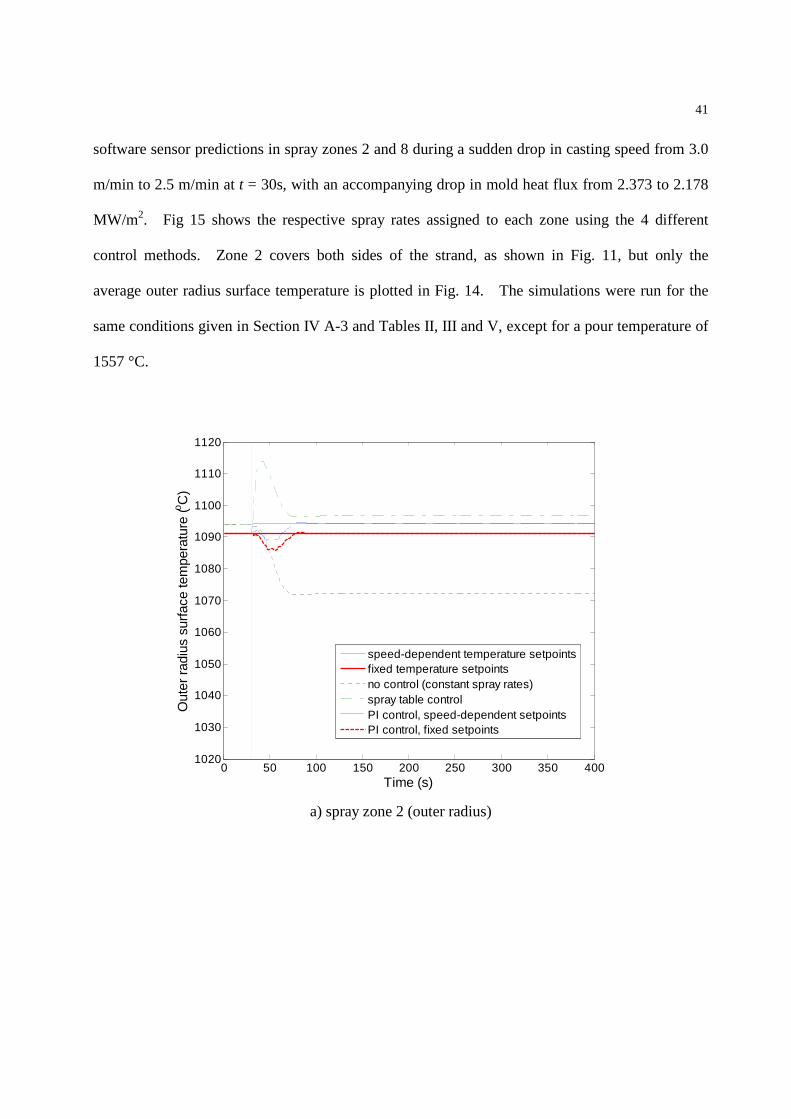
41
software sensor predictions in spray zones 2 and 8 during a sudden drop in casting speed from 3.0
m/min to 2.5 m/min at t = 30s, with an accompanying drop in mold heat flux from 2.373 to 2.178
MW/m2. Fig 15 shows the respective spray rates assigned to each zone using the 4 different
control methods. Zone 2 covers both sides of the strand, as shown in Fig. 11, but only the
average outer radius surface temperature is plotted in Fig. 14. The simulations were run for the
same conditions given in Section IV A-3 and Tables II, III and V, except for a pour temperature of
1557 °C.
0 50 100 150 200 250 300 350 4001020
1030
1040
1050
1060
1070
1080
1090
1100
1110
1120
Time (s)
Out
er r
adiu
s su
rfac
e te
mpe
ratu
re (o C
)
speed-dependent temperature setpointsfixed temperature setpointsno control (constant spray rates)spray table controlPI control, speed-dependent setpointsPI control, fixed setpoints
a) spray zone 2 (outer radius)

42
0 50 100 150 200 250 300 350 4001020
1030
1040
1050
1060
1070
1080
1090
1100
1110
1120
Time (s)
Out
er r
adiu
s su
rfac
e te
mpe
ratu
re (o C
)
speed-dependent temperature setpointsfixed temperature setpointsno control (constant spray rates)spray table controlPI control, speed-dependent setpointsPI control, fixed setpoints
b) spray zone 8
Figure 14. Zone-average temperatures during a sudden slowdown from 3.0 to 2.5 m/min casting speed, comparing four control methodologies.
With no controller, spray-water flow rates remain constant with time, so the decrease in casting
speed causes higher heat extraction at any given distance down the caster, and the surface
temperatures all eventually drop. The time delay for the transition to the new lower steady-state
temperature varies with distance down the caster. Steady state is not reached until steel starting
at the meniscus at the transition time (t = 30s) finally reaches the given point in the caster, after
being cast entirely under the new conditions. Thus, points nearer to the meniscus react quickly to
the change, while points lower in the caster are affected by the changing upstream temperature
history for a long time. In the figures, it is clear that zone 2 reaches steady state sooner than zone
8.

43
With a controller that increases spray water in proportion to casting speed, the responses in
Fig. 14 show a characteristic temperature overshoot before settling to steady state. During a
sudden speed drop, the spray rates drop immediately, as seen in Fig. 15. However, with the
recently higher casting speed, the upstream steel is hotter than expected, so the surface
temperatures overshoot the desired values at steady state. The steady-state temperatures at 2.5
m/min are larger than the steady-state temperatures at 3.0 m/min because the spray rates assigned
at the lower speed are predicted by the model to be even lower than the drop in speed requires.
0 50 100 150 200 250 300 350 4000
5
10
15
20
25
30
35
40
45
Time (s)
Spr
ay-w
ater
flux
Qsw
(L/
s/m
2 )
no control (constant spray rate)spray table controlPI control, speed-dependent setpointsPI control, fixed setpoints
Zone 8
Zone 2

44
Figure 15. Spray-water flow rates corresponding to Fig. 13 example during a sudden slowdown from 3.0 to 2.5 m/min casting speed, comparing 4 control methodologies.
With PI control using speed-dependent temperature setpoints, the overshoot is drastically
reduced. In fact, in Fig. 14a, it can be seen that there is initially a slight undershoot in zone 2.
As Fig 15 makes clear, this is because the spray flow rate command from the PI controller changes
more gradually than spray-table control. However, the command changes as sharply as spray-
table control in zone 8. This response is needed to achieve the larger change in temperature
setpoints at the speed change. The later small decrease before finally reaching steady state is
needed to avoid the overshoot.
Finally, these results illustrate the superiority of PI control using fixed temperature setpoints.
With this controller, the surface temperature is kept remarkably constant through the speed change.
To achieve this, Fig. 15 clearly shows how the sprays are gradually decreased after the speed
change, and the further the zone is from meniscus, the more gradually the spray rate is changed.
The steady-state spray-water flow rates are properly smaller at the lower casting speed.
This case study demonstrates that all of the controllers perform as expected. The PI
controller with fixed setpoints produces the best response for steel quality, as detrimental surface
temperature fluctuations are lessened. The quality of the control system now depends on the
accuracy of the software sensor calibration to match the real caster. Work is proceeding to
measure heat transfer, both with fundamental laboratory experiments, and with optical pyrometers
and other experiments in the commercial steel thin-slab caster.

45
VI. SUMMARY
Maintaining the shell surface temperature profile under transient conditions by spray-water
cooling in continuous casting of steel is important to minimize surface cracks. For this purpose, a
real-time spray-cooling control system, CONONLINE, is being implemented on a commercial
caster that includes 1) a software sensor for accurate estimation/prediction of shell surface
temperature, 2) control algorithm and data checking subroutines for robust temperature control, 3)
TCP/IP Server and Client programs for communicating between these two software components
and the caster, and 4) a real-time monitor to allow operator input and display the predicted shell
surface temperature profiles, water flow rates, and other important operating data. Simulation
results demonstrate that the new control system achieves better temperature control performance
than conventional systems, especially when using a new strategy to generate temperature setpoints
which vary according to the measured mold heat flux, and a controller with anti-windup that
maintains constant a surface temperature profile with casting speed.
ACKNOWLEDGEMENTS
Ron O’Malley, Matthew Smith, Terri Morris, and Kris Sledge from Nucor Decatur are
gratefully acknowledged for their unwavering support and help with this work. The TCP/IP
programs in CONONLINE were written by Rob Oldroyd from DBR Systems on behalf of Nucor
Decatur. We are grateful for work on CON1D calibration for the Nucor Decatur steel mill by
Sami Vahpalahti and Huan Li, from the University of Illinois. We are also very grateful for their
work on CONONLINE. This work is supported by the National Science Foundation under Grant
DMI 05-00453 and the Continuous Casting Consortium at UIUC.

46
NOTATION
0 superscript to indicate initial time of creation (at meniscus)
∆t time interval for control calculation (s)
i subscript for CON1D slice number, used in CONSENSOR (N total)
j subscript for spray zone number (Nzone total) Pjk , I
jk proportional, integral controller gains
l j total length of the area of the steel surface upon which all the sprays in zone j
impinge.
Lj total length of zone j
q surface heat flux at a particular time and location (MW/m2) q mold average steel surface heat flux in mold (MW/m2)
Qsw spray water flux (L/s/m2) on surface of steel
t real time (s)
ti(z) time at which slice i passes distance z from the meniscus
Ti(x,t) temperature of CON1D slice i: 1-D transverse cross-section moving along strand
centerline at Vc (°C)
Ts(z,t) strand surface temperature setpoint (°C)
T̂ (z,t) strand surface temperature estimate (°C)
uj′(t), uj(t) spray water flow rate: measured, requested controller output (L/s)
Vc casting speed (m/s)
x distance through thickness of strand (m)
z distance from meniscus, in casting direction (m)
zi(t) distance from meniscus of slice i at time t (m)

47
REFERENCES 1. J.K. Brimacombe, P.K. Agarwal, S. Hibbins, B. Prabhaker and L.A. Baptista: "Spray Cooling in Continuous
Casting," in Continuous Casting, vol. 2, J. K. Brimacombe, ed., 1984, pp. 105-123. 2. M. M. Wolf: Continuous Casting: Initial Solidification and Strand Surface Quality of Peritectic Steels, vol. 9,
Iron and Steel Society, Warrendale, PA, 1997, pp. 1-111. 3. K. Okuno, H. Naruwa, T. Kuribayashi and T. Takamoto: "Dynamic spray cooling control system for continuous
casting," Iron Steel Eng., 1987, vol. 64 (4), pp. 34-38. 4. K.-H. Spitzer, K. Harste, B. Weber, P. Monheim and K. Schwerdtfeger: "Mathematical model for thermal
tracking and on-line control in continuous casting," Iron Steel Inst. Jpn, 1992, vol. 32 (7), pp. 848-856. 5. S. Barozzi, P. Fontana and P. Pragliola: "Computer control and optimizationof secondary cooling during
continuous casting," Iron Steel Eng, 1986, vol. 63 (11), pp. 21-26. 6. B. Lally, L. Biegler and H. Henein: "Finite difference heat-transfer modeling for continuous casting," Met.
Trans. B, 1990, vol. 21 (4), pp. 761-770. 7. K. Dittenberger, K. Morwald, G. Hohenbichler and U. Feischl: "DYNACS Cooling Model - Features and
Operational Results," Proc. VAI 7th International Continuous Casting Conference, (Linz, Austria), 1996, pp. 44.1-44.6.
8. R.A. Hardin, K. Liu, A. Kapoor and C. Beckermann: "A Transient Simulation and Dynamic Spray Cooling Control Model for Continuous Steel Casting," Metal. & Material Trans., 2003, vol. 34B (June), pp. 297-306.
9. S. Louhenkilpi, E. Laitinen and R. Nienminen: "Real-time simulation of heat transfer in continuous casting," Metal. & Material Trans. B, 1999, vol. 24 (4), pp. 685-693.
10. S. Louhenkilpi, J. Laine, T. Raisanen and T. Hatonen: "On-Line Simulation of Heat Transfer in Continuous Casting of Steel," in 2nd Int. Conference on New Developments in Metallurgical Process Technology, (Riva del Garda, Italy, 19-21 Sept, 2004), 2004.
11. T. Raisanen, S. Louhenkilpi, T. Hatonen, J. Toivanen, J. Laine and M. Kekalainen: "A Coupled Heat Transfer Model for Simulation of Continuous Casting," in European Congress on Computational Methods in Applied Sciences and Engineering, 2004,
12. M. Jauhola, E. Kivela, J. Konttinen, E. Laitinen and S. Louhenkilpi: "Dynamic Secondary Cooling Model for a Continuous Casting Machine," Proc. 6th International Rolling Conference, (Dusseldorf; Germany, 20-22 June, 1994), 1994, vol. 1, pp. 196-200.
13. K. Zheng, B. Petrus, B.G. Thomas and J. Bentsman: "Design and Implementation of a Real-time Spray Cooling Control System for Continuous Casting of Thin Steel Slabs,," Proc. AISTech 2007, Steelmaking Conference Proceedings, Indianapolis, May 7-10, 2007, 2007.
14. Y. Meng and B.G. Thomas: "Heat Transfer and Solidification Model of Continuous Slab Casting: CON1D," Metal. & Material Trans., 2003, vol. 34B (5), pp. 685-705.
15. C. Edwards and I. Postlethwaitex: "Anti-windup and Bumpless Transfer Schemes," Proc. UKACC International Conference on CONTROL, 1996, pp. 394-399.
16. B. Santillana, L.C. Hibbeler, B.G. Thomas, A. Hamoen, A. Kamperman, W. van der Knoop: "Investigating Heat Transfer In Funnel-Mould Casting With CON1D: Effect of Plate Thickness," ISIJ Internat., 2008, vol. 48 (10), pp. 1380-1388.
17. J. Sengupta, M.-K. Trinh, D. Currey and B. Thomas: "Utilization of CON1D at ArcelorMittal Dofasco's No. 2 Continuous Caster for Crater End Determination," in AISTech 2009, (St. Louis, MO, USA), 2009, vol. 1, pp. 1177-1185.
18. Y.M. Won and B.G. Thomas: "Simple model of microsegregation during solidification of steels," Metallurgical and Materials Transactions A (USA), 2001, vol. 32A (7), pp. 1755-1767, 179.
19. Y. Meng and B.G. Thomas: "Modeling Transient Slag Layer Phenomena in the Shell/Mold Gap in Continuous Casting of Steel," Metall. Mater. Trans. B, 2003, vol. 34B (5), pp. 707-725.

48
20. J.-K. Park, B. G. Thomas, I. V. Samarasekera and U.-S. Yoon: "Thermal and Mechanical Behavior of Copper Moulds During Thin Slab Casting (I): Plant Trial and Mathematical Modelling," Metall. Mater. Trans., 2002, vol. 33B (June), pp. 425-436.
21. T. Nozaki: "A Secondary Cooling Pattern for Preventing Surfcace Cracks of Continuous Casting Slab," Trans. ISIJ, 1978, vol. 18, pp. 330-338, not labelled.
22. R.A. Hardin, H. Shen and C. Beckermann: "Heat Transfer Modeling of Continuous Steel Slab Caster Using Realistic Spray Patterns," Proc. Modelling of Casting, Welding and Advanced Solidification Processes IX, (Aachen, Germany), 2000, pp. 729-736, 190.
23. E. Mizikar: "Spray cooling investigation for continuous casting of billets and blooms," Iron Steel Engineer, 1970, vol. 47 (6), pp. 53-60.
24. L.K. Chiang: Proc. 57th Electric Furnace Conference, (Pittsburgh, USA), 1999. 25. K. Tanner: "Comparison of Impact, Velocity, Dropsize, and Heat Flux to Redefine Nozzle Performance in the
Caster," Proc. MS&T Conference Proceedings, B. G. Thomas, ed., (New Orleans, Sept 24-28, 2004), 2004. 26. K. Kasperski: "Spray Cooling Results of Air/Mist Spray Nozzles with Reduced Air Volumes," Proc. MS&T
Conference Proceedings, B. G. Thomas, ed., (New Orleans, Sept 24-28, 2004), 2004. 27. S.-M. Lee and S.-Y. Jang: ISIJ International (Japan), 1996, vol. 36 (Supplementary on Science and Technology
of Steelmaking), pp. 208-210. 28. S. Vapalahti, H. Castillejos, Andrés Acosta, Alberto C. Hernández and B.G. Thomas: "Delavan Nozzle
Characterization Research at CINVESTAV," 2007. 29. S. Vapalahti, H. Castillejos, Andrés Acosta, Alberto C. Hernández and B.G. Thomas: "Spray Heat Transfer
Research at CINVESTAV," 2007. 30. S. Vapalahti, B. G. Thomas, S. Louhenkilpi, A.H. Castillejos, F. A. Acosta and C. A. Hernandez: "Heat Transfer
Modelling of Continuous Casting: Numerical Considerations, Laboratory Measurements and Plant Validation," Proc. STEELSIM 2007, (Graz, Austria, Sept. 12-14, 2007), 2007.
31. J. Sengupta, M.-K. Trinh, D. Currey and B. G. Thomas: "Utilization of CON1D at ArcelorMittal Dofasco’s No. 2 Continuous Caster for Crater End Determination," Proc. AISTech 2009 Steelmaking Conference Proc., (St. Louis, MO, May 4-7, 2009), 2009, vol. 1.
32. Trico Steel L.L.C.: "Spray Nozzle Arrangement," 1995, (Internal Document, Nucor Steel, Decatur AL). 33. C. Brosilow and B. Joseph: Techniques of Model-Based Control, Prentice-Hall international series in the
physical and chemical engineering sciences Prentice Hall, Upper Saddle River, NJ, 2002. 34. Y. V. Orlov and M. V. Basin: "On Minmax Filtering Over Discrete-Continuous Observations," IEEE
Transactions on Automatic Control, 1995, vol. 40 (9). 35. C. Cicutti, M. Valdez, T. Perez, G.D. Gresia, W. Balante and J. Petroni: "Mould thermal evaluation in a slab
continuous casting machine," Proc. 85th Steelmaking Conference, (Nashville, TN, USA), 2002, vol. 85, pp. 97-107, 282.