Embed Size (px)
Citation preview
Real-time HV OHTL sag monitoring
system based on Power Line Carrier
signal behaviour
Wernich de Villiers
December 2005
Supervisor: Professor J.H. Cloete
Dissertation presented for the Degree of Doctor of Philosophy in Electrical
Engineering at the University of Stellenbosch.

Declaration
I, the undersigned, hereby declare that the work contained in this
dissertation is my own original work and that I have not previously in its
entirety or in part submitted it at any university for a degree.
W de Villiers: ________________________
Date: ________________________
ii

Summary
A new method of measuring the change in the average height of phase
conductors above the ground plane of High Voltage (HV) Overhead
Transmission Lines (OHTLs) was discovered in 1999, at Stellenbosch
University. The new method, called Power Line Carrier–Sag (PLC-SAG),
measures average overhead conductor height variations in real-time by
exploiting high frequency signal propagation characteristics on the
existing PLC system.
The novelty of the newly discovered PLC-SAG system naturally led to a
thorough testing and investigation of the technique. This thesis explains
the methodology used to produce unique experimental data, which has
indeed proven that the average height of an OHTL can be tracked very
accurately via the PLC-SAG technique for continuous periods.
As the experiments on two live 400 kV transmission lines in South Africa
were being undertaken, a serious concern regarding the new technique
arose. Major HV Station impedance variations seemed to influence the
PLC system and clouded the interpretation of PLC-SAG recorded data.
Such HV Station impedance variations typically occur only a few times per
year.
A new Power Line Carrier Impedance (PLC-IMP) technique was then
discovered, by which these changes could be monitored. No structural
changes to the existing PLC-SAG system were required for this technique.
This was seen as a major breakthrough in the presented study. Not only
does this newly established technique make it possible to develop a stable
PLC-SAG system, but also a potential real-time condition monitor
application. Its use on PLC systems has been proposed to the main Power
Utility in South Africa.
iii
Opsomming
‘n Nuwe metode om die veranderinge in die gemiddelde hoogte bo
grondvlak van die fasegeleiers van hoogspanning oorhoofse
transmissielyne te meet is in 1999 by die Universiteit Stellenbosch ontdek.
Hierdie uitvindsel staan bekend as die Power Line Carrier Sag (PLC-SAG)
metode en dit meet veranderinge in oorhoofse geleier hoogte intyds deur
benutting van die eienskappe van hoëfrekwensie sein voortplanting op die
bestaande hoogspanning oorhoofse transmissielyne.
Die nuutuitgevonde PLC-SAG stelsel is natuurlik onderworpe aan
deeglike toetsing en ondersoek van die tegniek. Hierdie proefskrif
verduidelik die metodiek gebruik, waarvolgens unieke eksperimentele
data verkry is wat bewys dat die gemiddelde hoogte van ‘n hoogspannings
oorhoofse transmissielyn inderdaad baie akkuraat gemeet kan word, oor
lang ononderbroke tydperke.
Tydens die eksperimente en ondersoek op twee lewendige 400kV
transmissielyne in Suid Afrika is ‘n ernstige probleem gewaar wat die
vatbaarheid van die tegniek in gevaar gestel het. Groot verskille in
impedansie by hoogspanningstasies beïnvloed die hoogspanning oorhoofse
transmissielyn stelsel en versteur die interpretasie van die PLC-SAG data
wat opgeneem is. Sulke groot impedansie verskille kom tipies slegs ’n paar
keer per jaar by ‘n stasie voor.
‘n Tweede nuwe tegniek, die sogenoemde Powerline Carrier Impedance
(PLC-IMP) tegniek, is toe ontdek wat hierdie veranderinge kan monitor en
dus die intydse hoogspannings oorhoofse transmissielyne impedansie
metings moontlik maak. Geen struktuurverandering van die bestaande
PLC-SAG stelsel is nodig vir gebruik van die PLC-IMP tegniek nie, en dit
word beskou as ‘n groot deurbraak in die studie wat hier aangebied word.
iv

Hierdie tegniek het teweeggebring nie slegs ‘n stabiele PLC-SAG stelsel
nie, maar ‘n potensiële intydse monitor vir gebruik op hoogspannings
oorhoofse transmissielyn stelsels. Die tegniek is voorgestel aan die
grootste kragvoorsiener in Suid Afrika vir gebruik op hul stelsels.
v

Acknowledgements
Soli Deo Gloria
I am greatly indebted to my supervisor, Prof JH Cloete, for sharing his
expertise, for giving guidance and for his ever-present optimism. I would
also especially like to thank Eskom/TAP, particularly Mr A Burger and Mr
DC Smith as well as Prof LM Wedepohl. Furthermore I would also like to
thank the following people for their support and help:
From Eskom Transmission Telecommunications: Frans Venter, Piet
Lubbe, Drikus de Wet, Errol Wright, Tony Pereira and Ashley van der
Poel.
From Trans Africa Projects TAP/Eskom: Johan Cloete, Dr D Muftic, Pieter
Pretorius, Nick Kruger, Hein Pienaar and Sarel Cloete.
From Stellenbosch University: Prof HC Reader, Dr RG Urban and Anita
van der Spuy.
The financial assistance of the Department of Labour (DoL), Harry
Crossley Scholarship and TAP/Eskom towards this research is hereby
acknowledged. Opinions expressed and conclusions arrived at, are those of
the author and are not necessarily to be attributed to the DoL.
Finally, special thanks to my wife, family and friends for their continuous
support.
vi
Table of contents
Declaration .................................................................................................... ii
Summary ...................................................................................................... iii
Opsomming....................................................................................................iv
Acknowledgements........................................................................................vi
Table of contents...........................................................................................vii
List of figures.............................................................................................. xiii
List of photographs......................................................................................xix
Chapter 1 Introduction and background ..............................................1
1.1 Introduction ...........................................................................................1
1.2 Ampacity systems..................................................................................2
1.2.1 Introduction and literature review of Ampacity systems ..............2
1.2.2 History of the fundamental idea on which PLC-SAG is based......4
1.2.3 Comparison of PLC-SAG with other Ampacity techniques ...........5
1.3 The goals of this study ..........................................................................6
1.3.1 PLC-SAG system development .......................................................7
1.3.2 PLC-SAG evaluation .......................................................................7
1.4 Thesis layout and original contributions..............................................8
1.4.1 Chapter 2: The Power Line Carrier (PLC) system.........................8
1.4.2 Chapter 3: Simulation of the two case studies and frequency
allocation of the PLC-SAG monitoring tones ..........................................9
1.4.3 Chapter 4: PLC-SAG experimental installations...........................9
1.4.4 Chapter 5: Direct height measurements ......................................10
1.4.5 Chapter 6: PLC-SAG system evaluation and calibration ............10
1.4.6 Chapter 7: PLC-SAG impedance monitoring system...................11
1.4.7 Chapter 8: Conclusions .................................................................12
1.5 Conclusion............................................................................................12
References.....................................................................................................12
Chapter 2 The Power Line Carrier (PLC) system .............................14
2.1 Introduction .........................................................................................14
2.2 Overview of the PLC system [1]..........................................................14
vii

2.3 The theory of natural modes [2][3][4][5].............................................18
2.3.1 Voltage propagation matrix ..........................................................18
2.3.2 Eigenvectors of the voltage propagation matrix ..........................19
2.3.3 Eigenvalues of the voltage propagation matrix ...........................22
2.3.4 Multi-Conductor Wave equation...................................................23
2.4 PLC – SAG model development ..........................................................25
2.4.1 Model definitions ...........................................................................27
2.4.2 Database (Microsoft Access, left-hand side of Figure 2.5) ...........30
2.4.3 Input/Output ranges and (Matlab) GUI.......................................31
2.5 New average ground resistance estimation technique for PLC signal
attenuation simulations ............................................................................34
2.5.1 Introduction ...................................................................................34
2.5.2 Theory ............................................................................................35
2.5.3 Simulations and average ground resistivity for the PLC link
between Kriel power station and Tutuka power station. .....................36
2.5.4 Comparing the technique with other techniques.........................43
2.6 Conclusion............................................................................................44
References.....................................................................................................44
Chapter 3 Simulation of the two case studies and frequency
allocation of the PLC-SAG monitoring tones .....................................46
3.1 Introduction .........................................................................................46
3.2 Locations of the two OHTL sites.........................................................47
3.2.1 General...........................................................................................47
3.2.2 Case Study 1: Koeberg-Acacia (KA)..............................................48
3.2.3 Case Study 2: Kriel-Tutuka (KT)..................................................49
3.3 Simulations..........................................................................................52
3.3.1 General...........................................................................................52
3.3.2 Case 1: Koeberg-Acacia .................................................................53
3.3.3 Case Study 2: Kriel-Tutuka ..........................................................57
3.4 Choosing PLC-SAG tones....................................................................62
3.4.1 General...........................................................................................62
3.4.2 Case study 1: Koeberg-Acacia .......................................................64
viii

3.4.3 Case study 2: Kriel-Tutuka...........................................................65
3.5 Conclusion............................................................................................67
References.....................................................................................................67
Chapter 4 PLC-SAG experimental installations ................................69
4.1 Introduction .........................................................................................69
4.2 Measuring Hybrid (to incorporate outer phase to outer phase
coupling).....................................................................................................71
4.3 Case 2: Transmitter at Tutuka Power Station...................................75
4.3.1 Transorb.........................................................................................77
4.3.2 Amplifier ........................................................................................77
4.3.3 Attenuator in the transmitter circuit ...........................................78
4.3.4 Signal generator under computer control.....................................80
4.4 Case 2: Receiver at Kriel Power Station ............................................81
4.4.1 Attenuator in the receiver circuit .................................................82
4.4.2 Receivers ........................................................................................83
4.4.3 Receiver control program ..............................................................84
4.4.4 Industrial cell phone......................................................................87
4.5 Conclusions ..........................................................................................88
References.....................................................................................................88
Chapter 5 Direct height measurements...............................................89
5.1 Introduction .........................................................................................89
5.2 Different instruments considered for the direct height measurements
....................................................................................................................90
5.2.1 Setup for the direct height measurement.....................................91
5.2.2 Measurements ...............................................................................91
5.2.3 Conclusion of the OHTL conductor height measurement trial ...93
5.3 The measurement methodology..........................................................94
5.4 Step 1: Site selection ...........................................................................95
5.4.1 Case 1: Koeberg-Acacia (KA) ........................................................96
5.4.2 Case 2: Kriel-Tutuka (KT).............................................................97
5.5 Step 2: Marking measurement points at selected sites .....................98
5.6 Step 3: Measurement site survey .....................................................100
ix
5.7 Step 4: Performing the direct height measurement.........................102
5.7.1 Case study: KA (Direct height measurement above peg) ..........104
5.7.2 Case study: KT (Direct height measurement above peg) .........105
5.8 Transforming to the average height .................................................106
5.9 Conclusions ........................................................................................110
References...................................................................................................110
Chapter 6 PLC-SAG system evaluation and calibration ................111
6.1 Introduction .......................................................................................111
6.2 Case study 1 (Koeberg-Acacia) logged tones ....................................112
6.2.1 Logged PLC-SAG monitoring tones............................................112
6.2.2 General comments about the logged data ..................................113
6.2.3 Levels of the received PLC-SAG tones .......................................114
6.2.4 Variation of the received PLC-SAG tones compared with the
simulations ...........................................................................................116
6.2.5 Correlation between direct height measurement and the logged
attenuation values for KA....................................................................118
6.3 Case study 2 (Kriel-Tutuka) logged tones ........................................121
6.3.1 Logged PLC-SAG monitoring tones............................................121
6.3.2 General comments about the logged data ..................................122
6.3.3 Levels of the received PLC-SAG tones .......................................123
6.3.4 Variation of the received PLC-SAG tones compared to the
simulations ...........................................................................................124
6.3.5 Correlation between direct height measurement and the logged
attenuation values for KT ....................................................................126
6.4 Calibration of the PLC-SAG system.................................................129
6.4.1 Case study 1 (Koeberg-Acacia)....................................................130
6.4.2 Case study 2 (Kriel-Tutuka) .......................................................134
6.5 Conclusions ........................................................................................136
References...................................................................................................137
Chapter 7 PLC-SAG impedance monitoring system .......................138
7.1 Introduction .......................................................................................138
7.2 Logged received levels with unexpected step effect in data ............139
x

7.3 Background theory of hybrid applied to the PLC System ...............143
7.4 Isolation of a hybrid...........................................................................146
7.4.1 Isolation .......................................................................................147
7.4.2 Simulations..................................................................................149
7.4.3 Insertion loss laboratory experiment..........................................151
7.5 PLC impedance (PLC-IMP) monitoring system...............................153
7.5.1 Monitoring the PLC impedance at the carrier frequency..........153
7.5.2 Monitoring the PLC impedance at different frequencies...........155
7.6 Transmission line and station impedance........................................156
7.6.1 Identifying PLC related impedances ..........................................157
7.6.2 PLC-IMP sensitivity analysis .....................................................158
7.6.3 Preliminary impedance monitoring experiment ........................161
7.7 Conclusion..........................................................................................162
References...................................................................................................163
Chapter 8 Conclusions and Recommendations ...............................164
8.1 Conclusions ........................................................................................164
8.2 Recommendations..............................................................................165
8.2.1 Mode 1: PLC-IMP at Station A ...................................................168
8.2.2 Mode 2: PLC-SAG A to B ............................................................168
Appendix A OHTL and PLC system details for the two case
studies .......................................................................................................169
A.1 Introduction ......................................................................................169
A.2 Koeberg-Acacia OHTL ......................................................................170
A.3 Koeberg-Acacia PLC system.............................................................172
A.4 Kriel-Tutuka OHTL..........................................................................173
A.5 Kriel-Tutuka PLC System................................................................183
Appendix B Additional information about Koeberg-Acacia and
Kriel-Tutuka operational PLC’s ..........................................................184
B.1 Introduction ......................................................................................184
B.2 Acacia-Koeberg neighbouring PLC frequencies ..............................186
B.3 Navigational Radio Beacon Frequencies (053/1839) .......................187
B.4 Koeberg-Acacia frequency scan........................................................188
xi

B.5 Kriel-Tutuka neighbouring PLC frequencies (See paragraph B.1 for
colour definitions) ....................................................................................189
B.6 Kriel-Tutuka frequency scan............................................................190
Appendix C Additional information about the experimental
transmitter and receiver installations...............................................193
C.1 Introduction ......................................................................................193
C.2 Transorb datasheet...........................................................................193
C.3 Amplifier ...........................................................................................194
C.4 Impedance matching network and attenuator ................................195
C.5 Receiver settings for PLC-SAG tone monitoring.............................198
Appendix D PLC tone during the outage on the KT OHTL dated
2004/05/04 ..................................................................................................199
D.1 Introduction ......................................................................................199
D.2 The 5 relevant tones .........................................................................200
xii
List of Figures
Figure 2.1 Simplified PLC system between two Stations...........................15
Figure 2.2 Coupling notation (Vp1,Vp2,Vp3) on a flat configuration OHTL
.................................................................................................................20
Figure 2.3 Graphical representation of the Modal distribution for a
differentially coupled signal...................................................................21
Figure 2.4 Typical attenuation constants for the different modes. (9 m-
phase spacing, 19.6 m conductor height, twin dinosaur phase
conductor type and 300 ohm-meter ground resistance)........................23
Figure 2.5 High level representation of the simulation model...................26
Figure 2.6 Defining an Overhead Transmission Line (OHTL) span
between two adjacent towers for a special case (equal attachment
height and horizontal ground) ...............................................................27
Figure 2.7 Average conductor height...........................................................29
Figure 2.8 Input parameters for the Microsoft Database...........................31
Figure 2.9 Snapshot of the PLC-SAG simulation program output display34
Figure 2.10 Kriel-Tutuka OHTL .................................................................37
Figure 2.11 Different simulated attenuations on the Kriel-Tutuka
transmission line for 50 ohm-meter ground resistance ........................39
Figure 2.12 Measurement and simulation for standard coupling
configurations (Equation 2.19)...............................................................41
Figure 2.13 Measurement and simulation for outer phase to outer phase
(Equation 2.20) .......................................................................................41
Figure 2.14 Measurement and simulation for centre phase to centre phase
(Equation 2.20) .......................................................................................42
Figure 2.15 Measurement and simulation for outer phase to centre phase
(Equation 2.21) .......................................................................................42
Figure 2.16 Measurement and simulation for centre phase to outer phase
(Equation 2.22) .......................................................................................43
Figure 3.1 Map of Koeberg-Acacia OHTL ...................................................48
Figure 3.2 Map of Kriel-Tutuka OHTL .......................................................50
xiii
Figure 3.3 Seven sections of the OHTL.......................................................51
Figure 3.4 Ruling span of Koeberg-Acacia OHTL (Table 3.3) ....................53
Figure 3.5 Koeberg-Acacia default simulation condition for the various
coupling configurations (solid line) and two meter sagged conductor
(dotted line). Ground resistivity equals 150 ohm meter. ......................55
Figure 3.6 Expected PLC-SAG tone variation with average height for
Outer phase to Outer phase coupling on Koeberg-Acacia OHTL.........57
Figure 3.7 Ruling span of Kriel-Tutuka transmission line ........................58
Figure 3.8 Default simulation condition for the various coupling
configurations (solid line) and conductor sagged by two meters (dotted
line) .........................................................................................................60
Figure 3.9 Expected PLC-SAG tone variation with average height for
Outer phase (white phase at Kriel, Figure 2.9) to Outer phase (blue
phase at Tutuka) coupling on Kriel-Tutuka OHTL ..............................61
Figure 3.10 Frequency scan of the Koeberg-Acacia 400 kV OHTL
performed at Acacia Sub Station ...........................................................65
Figure 3.11 Frequency scan Kriel-Tutuka 400 kV OHTL performed at
Kriel Power Station. ...............................................................................66
Figure 4.1 Simplex logging system. Dedicated Transmit and Receive PLC-
SAG units................................................................................................70
Figure 4.2 Duplex logging system. Identical Transmit and Receive PLC-
SAG units................................................................................................70
Figure 4.3 Normal PLC system with the hybrid.........................................72
Figure 4.4 Measurement Hybrid for the PLC-SAG system........................73
Figure 4.5 Layout of the stand-alone installation at Tutuka PS ...............76
Figure 4.6 Impedance of the amplifier (red circle) and the impedance of
the amplifier via a 10 dB attenuator (blue circle).................................79
Figure 4.7 Layout of the stand-alone installation at Kriel Power Station 81
Figure 4.8 Steps in the measurement cycle, which measure noise and the
received level. .........................................................................................85
Figure 5.1 Conductor heights, measured on Saturday 26 April 2003, via
the four different instruments ...............................................................92
xiv

Figure 5.2 Locations of the calibration points on the 400 kV Koeberg-
Acacia transmission line as a function of length. .................................97
Figure 5.3 Locations of the calibration points on the 400 kV Kriel-Tutuka
transmission line. ...................................................................................98
Figure 5.4 Dimensions of a typical span ...................................................101
Figure 5.5 Measurement set-up at a site ..................................................103
Figure 5.6 Direct height measurement above the pegs of KA..................104
Figure 5.7 Measured height variation at the three KT calibration sites
(2004/05/04) and (2004/05/06) ..............................................................105
Figure 5.8 Layout of KA - CA1 and measurement point ..........................106
Figure 5.9 Average height movement of the conductor above a perfect
ground plane for the calibration point KA - CA1 ................................107
Figure 5.10 Estimated average height variation of the KA OHTL (Case
study 1) .................................................................................................108
Figure 5.11 Estimated average height variation of the KT OHTL (Case
study 2) .................................................................................................109
Figure 6.1 Attenuation variation of all ten tones on KA PLC-SAG system.
Measurement days 1 and 2 are indicated by the red squares in the
data (Specific configuration is specified in Appendix C).....................113
Figure 6.2 KA OHTL attenuation simulation as a function of average
conductor height for Tone 3 and Tone 10. ...........................................116
Figure 6.3 Best correlated tones for KA PLC-SAG system ......................120
Figure 6.4 The principal PLC-SAG tones for the KA system...................121
Figure 6.5 Signal level variation of all ten tones on KT PLC-SAG system.
Measurement days 1 and 2 are indicated by the red squares (Measured
with Wandel & Goltermann selective voltmeter)................................122
Figure 6.6 KT OHTL attenuation simulation as a function of average
conductor height for Tone 3 and Tone 10. ...........................................124
Figure 6.7 Best 3 correlated tones for KT PLC-SAG system measured with
the W&G receiver .................................................................................128
Figure 6.8 The principal PLC-SAG tone for KT (Average of the 3 best
correlated KT PLC-SAG tones)............................................................129
xv

Figure 6.9 Theoretical calibration curve for the principal PLC-SAG tone
for the KA OHTL. .................................................................................130
Figure 6.10 Calibrated PLC-SAG signal and the measured average height
of the conductor for KA (Correlation = 99.02%) .................................133
Figure 6.11 Theoretical calibration curve for the principal PLC-SAG tone
for the KT OHTL. .................................................................................134
Figure 6.12 PLC-SAG AHS and the measured average height of the
conductor (Correlation = 97,38%) for KT.............................................136
Figure 7.1 Logged KA PLC-SAG tones during 2004/09/17.......................139
Figure 7.2 Simplistic electrical diagram showing the two 500 MVA
transformers at Acacia Sub Station ....................................................141
Figure 7.3 Effect on signal level due to variation in station impedance
(Outer phase to Outer phase coupling on KA system)........................142
Figure 7.4 Circuit diagram of a hybrid......................................................143
Figure 7.5 Odd mode excitation of hybrid .................................................148
Figure 7.6 Even mode excitation of hybrid ...............................................148
Figure 7.7 Isolation between Port 2 and Port 3 as a function of resistance
for an ideal hybrid ................................................................................149
Figure 7.8 Real part of the complex isolation for a complex Z1 for an ideal
hybrid ....................................................................................................150
Figure 7.9 Imaginary part of the complex isolation for a complex Z1 for an
ideal hybrid...........................................................................................151
Figure 7.10 Experimental results and simulations of isolation for different
values of resistance at Port 1 at 250 kHz. The exact resistance values
are 17.7, 47.7, 67, 74.3, 81.15, 98.4, 149 and 270 ohms as measured on
a bridge. ................................................................................................152
Figure 7.11 Measurement Hybrid which monitors the PLC impedance on
the outer phase at carrier frequencies.................................................154
Figure 7.12 Logging complex isolation at the Measurement Hybrid at any
frequency in the PLC band ..................................................................156
Figure 7.13 Impedance variations in the PLC system .............................157
Figure 7.14 Impedances at Acacia’s outer phase ......................................159
xvi

Figure 7.15 Measured variations in the magnitude of the insertion loss
over a period of one week on the KA OHTL ........................................162
Figure 8.1 Proposed setup for newly designed prototype units................167
Figure A.1 OHTL details of Koeberg-Acacia .............................................170
Figure A.2 LME strapping at Koeberg and Acacia for a standard
(“Electrisk Bureau” LME) ....................................................................173
Figure A.3 Section A of KT ........................................................................173
Figure A.4 Section B of KT ........................................................................174
Figure A.5 Section C of KT ........................................................................175
Figure A.6 Section D of KT ........................................................................175
Figure A.7 Section E of KT ........................................................................176
Figure A.8 Section F of KT.........................................................................176
Figure A.9 Section G of KT ........................................................................177
Figure A.10 LME strapping at Kriel and Tutuka.....................................183
Figure B.1 Part (Western Cape) of the Navigational Radio Beacon
Frequencies map in South Africa (053/1839) ......................................187
Figure B.2 100-520 kHz wideband measurement at Acacia Sub Station
(2004/03/18-2004/03/19). See Table B.1 and Figure B.1 for symbol
definition...............................................................................................188
Figure B.3 40-520 kHz wideband measurement at Kriel PS (2004/03/19-
2004/03/20)............................................................................................190
Figure B.4 Zoomed frequency scan of the Kriel-Tutuka 400 kV PLC link
(270 kHz – 290 kHz) (Tone 1) ..............................................................191
Figure B.5 Zoomed frequency scan of the Kriel-Tutuka 400 kV PLC link
(318 kHz – 350 kHz) (Tones 2-6)..........................................................191
Figure B.6 Zoomed frequency scan of the Kriel-Tutuka 400 kV PLC link
(460 kHz – 500 kHz) (Tones 7-10)........................................................192
Figure C.1 Impedance matching network (and 10 dB attenuator)
illustrating the design criteria.............................................................196
Figure C.2 Circuit layout of the impedance matching circuit ..................196
Figure D.1 Tone 3 - 2.653 dB added during the period of the outage ......200
Figure D.2 Tone 4 - 2.671 dB added during the period of the outage ......200
xvii

Figure D.3 Tone 5 - 2.975 dB added during the period of the outage ......201
Figure D.4 Tone 6 - 2.031 dB added during the period of the outage ......201
Figure D.5 Tone 9 - 0.4325 dB added during the period of the outage ....202
xviii

List of photographs
Photograph 2.1 Line Trap (LT), Capacitor Voltage Transformer (CVT) and
Line Matching Equipment (LME) .........................................................16
Photograph 4.1 Installation of a measurement hybrid...............................75
Photograph 4.2 An HP3336A signal generator together with an HP85
computer in the Lab ...............................................................................80
Photograph 4.3 The HP 3586A (left/bottom) and Wandel & Goltermann
PSM-137 (left/top) under computer control - testing the system. ........83
Photograph 5.1 Four instruments (from left to right) Theodolite, Laser
meter (Disto), Laser meter (Trimble) and Ultrasonic meter
(Suparuler)..............................................................................................90
Photograph 5.2 Three measurement stations .............................................91
Photograph 5.3 ‘Disto™ pro’ laser with telescopic viewer ..........................94
Photograph 5.4 Bushnell range finder ........................................................99
Photograph 5.5 Showing a peg made of railway sleeper (used as the lower
‘fixed’ point) together with the laser meter ...........................................99
Photograph 5.6 Location where the conductor height was measured – the
red dot on the outer phase of the conductor. (Used as the upper ‘fixed’
point) .....................................................................................................100
Photograph 5.7 Mr P Pretorius recording the measurements at KT CA2
with the GPS located on the table for GPS time.................................103
Photograph C.1 Transorb from Clear Line (Model 12-00109) ..................193
Photograph C.2 Amplifier from Mini-Circuits (model ZHL-32A)............194
xix
Chapter 1
Introduction and background
1.1 Introduction
The Power Line Carrier-Sag (PLC-SAG) system measures average
overhead conductor height variations in real-time. Knowledge of the
average conductor height variation can be used in Ampacity control
systems.
The PLC-SAG system is fundamentally based on the theory of Natural
Modes in Multi Conductor Transmission Lines [1]. The Monitoring PLC-
SAG tones are uniquely coupled via the existing Power Line Carrier (PLC)
infrastructure to the overhead transmission line. These coupled PLC-SAG
tones distribute into natural modes, which propagate to the remote
station. At the remote station these tones are decoupled and analysed to
extract information about the physical height of the overhead conductor.
The reader is further introduced to the research topic in Subsection 1.2,
which gives more background about Ampacity, available Ampacity
systems, history of the PLC-SAG system and comparisons between PLC-
SAG and other Ampacity systems.
The author has done a theoretical study [2] on the PLC-SAG technique,
with accompanying preliminary experiments. The goals of the research
presented (Subsection 1.3) in this thesis, were to thoroughly test the PLC-
SAG technique and to further develop the system for implementation.
1
These goals were achieved by designing and implementing PLC-SAG
monitoring systems onto two Over Head Transmission Lines (OHTLs).
The PLC-SAG system measures the average height of the OHTL
conductor, and in order to test the system a unique direct OHTL conductor
height experiment was planned and executed. From these experiments
the performance of the PLC-SAG system was quantified and areas of
concern were identified.
Subsection 1.4 describes the thesis layout and highlights the new key
contributions.
1.2 Ampacity systems
1.2.1 Introduction and literature review of Ampacity systems
The ampacity of an OHTL is defined as the maximum current flowing in
an OHTL that is consistent with safe operation [3].
Regulation [4] requires that transmission lines must be operated safely at
all times. The primary limitation on OHTL ampacity is maintaining the
design sags of the line under all operating conditions.
Environmental factors (for example temperature, wind and solar
radiation) contribute, together with the current in the conductor, to the
extent to which the transmission line conductor sags. Conservative
Electrical Power companies would assume worst-case values for the
environmental factors in order to determine the maximum current that
will ensure safe operation. This rating is called the static ampacity rating
[3] of the OHTL. In the competitive markets and fast growing demand
which some Electrical Power companies are experiencing, it is not
practical to operate the power grid on static ampacity ratings. By
2
monitoring the environmental effects, or the real-time sag of the
transmission line, the current rating of the OHTL could be increased
without compromising safety. This is called dynamic ampacity rating [3].
For example: On a cold winter day the ampacity rating will be higher than
on a hot summer day, because more current can be transferred on a cold
day before exceeding the sag limitations.
For Real Time dynamic line rating systems, continuous monitoring of
OHTL conditions is needed. Parameters that could be monitored are
current, weather related factors, conductor temperature and conductor
sag. There are a number of operational systems, which each use either
one or a combination of the mentioned parameters. For example:
• Real Time Thermal Rating System (RTTRS) [5] – Monitors the
temperature of the conductor
• ATLAS [6] – Monitors the ambient temperature
• Tension Monitoring System [7] – Monitors the sag via a strain gauge
• LINEAMPS [8] – Monitors weather conditions
• RETMOS [9] - Monitors weather conditions and sag conditions
Due to the nature of dynamic ampacity control, most of the above systems
incorporate some statistical techniques to compute the final estimated
ampacity of the transmission line.
The author, in collaboration with Prof JH Cloete [2][9][10], invented a
unique ampacity system called PLC-SAG. The history of the PLC-SAG
initiative and subsequent developments will be discussed in the following
section. This is done in order to put the research presented in this
document in perspective.
3

1.2.2 History of the fundamental idea on which PLC-SAG is based
Prof LM Wedepohl (Emeritus Dean of Applied Science University of
British Columbia) visited the University of Stellenbosch (US) during early
1999. Prof Wedepohl had discussions with Prof JH Cloete of the
Department of Electrical & Electronic Engineering, sharing his experience
on PLCs and a phenomenon called modal cancellation [1]. The
phenomenon was a function of the average conductor height.
Later that same year the author suggested the investigation of ampacity
and the possibility of monitoring sag through high frequency effects to
Prof Cloete. The discussion with Prof Cloete then guided the author to
thoroughly investigate the modal cancellation phenomenon which had
been mentioned by Prof Wedepohl.
The author completed an undergraduate project in 1999 [10] with the
initial simulations, which confirmed that there is an expected relationship
between PLC-signal attenuation and OHTL conductor sag.
The main goal of the author’s MScEng degree (2000-2001) [2] was to
develop a detailed simulation program to explore the concept in more
detail.
Due to extremely favourable results from the simulations and preliminary
single tone experiments, it was decided to continue the work on PLC-SAG
Ampacity.
The research presented in this thesis was the detailed continuation of the
author’s MScEng investigations with more emphasis on thorough
evaluation and practical system development.
4

Mr A Burger, a senior engineer at TAP (Trans Africa Project, a
subdivision of ESKOM enterprises) and his colleagues supported the
continuation of the work with financial and manpower resources during
2003 and 2004. Mr DC Smith, a Corporate Consultant at Eskom
transmission, and the Transmission Technology Department – Power
Telecommunication section which also supported the work with equipment
and skilled human resources from the start of the research. The research
was integrated with TAP’s existing RETMOS [9] ampacity research
program.
1.2.3 Comparison of PLC-SAG with other Ampacity techniques
The ampacity systems mentioned in Subsection 1.2.1 only estimate the
sectional sag in general, therefore numerous sensors are needed to
monitor the average sag of the whole transmission line. The unique
technical advantage of the PLC-SAG ampacity system is the fact that the
average value of the sag is measured. This is a key distinguishing feature
of the method.
The PLC-SAG system also has a significant competitive advantage in
terms of installation and operating costs. The aforementioned methods use
one or more loggers, which are installed on towers, conductors or near the
OHTL. The logged information must then be transmitted from the loggers,
which are typically in the middle of the transmission line, to the relevant
substation. Due to the fact that these loggers are likely to be in a rural
area, data transmission and maintenance becomes problematic, unreliable
and very expensive.
By contrast, the PLC-SAG system uses mainly the existing PLC
infrastructure. The Power Utility presently maintains this system. Only a
few hardware components have to be added to the existing PLC system to
5

realize ampacity control; no data have to be transmitted to the substation
and due to the sheltered environment of the substation, minimal
maintenance is required.
The main disadvantage of the PLC-SAG system is that it depends on the
existence of a PLC system. PLC systems are commonly installed on high
voltage transmission line networks and less commonly on the distribution
networks.
The fact that the average sag is measured can also be seen as a
disadvantage if the PLC-SAG ampacity system is the only ampacity
technique installed onto a particular OHTL. However, on a relatively
short OHTL a stand-alone PLC-SAG system may be adequate in many
cases.
The fact that the average sag is measured by use of a completely different
measuring technique is an advantage, especially when the technique is
used with a complementary technique which measures only the sectional
sag, which makes it possible to utilize different technologies on the same
transmission line and thus increase the confidence levels of the system
operators.
The RETMOS system [9] is ESKOM’s (main electrical power company in
South Africa) Real Time ampacity monitoring system. The PLC-SAG
technique is already recognized as one of the three fundamental
techniques in the RETMOS system, which is still under development.
1.3 The goals of this study
The goals of the study were to thoroughly test the PLC-SAG technique and
to further develop the technique for implementation in the field.
6

1.3.1 PLC-SAG system development
In [2] a preliminary single tone test was used to evaluate the performance
of the PLC-SAG system. The PLC-SAG system in this study was further
developed to a multi-tone monitoring system.
During the execution of the evaluation process (Section 1.3.2) the PLC-
SAG system developed. The two biggest developments were:
1- Calibration procedure for the PLC-SAG system via direct height
measurement
2- PLC Impedance monitoring (PLC-IMP) [12] technique, which is
essential for the reliable operation of the PLC-SAG system.
These developments will be explained in more detail.
1.3.2 PLC-SAG evaluation
The methodology used in [2] to test the single tone PLC-SAG system was
compared against another Ampacity system, which uses current and
weather factors to compute the Ampacity on one OHTL. The problem with
this other technique is that the Ampacity system is based on assumptions
and does not produce an exact value. It is therefore very difficult to
compare the systems, because the exact values are unknown.
After some consideration it was decided to perform a dedicated unique
experiment to test the performance of the PLC-SAG system. Due to the
fact that the PLC-SAG system measures the average height of the whole
transmission line, it was decided to measure the height of the OHTL
conductor directly at three well-spaced locations. By comparing the results
7

from the direct height experiment with the results from the PLC-SAG
system the level of accuracy of the system could be determined.
These experiments were done on two live 400 kV OHTLs in South Africa.
1.4 Thesis layout and original contributions
1.4.1 Chapter 2: The Power Line Carrier (PLC) system
The existing PLC system is introduced by describing its functionality in
the power network and the working of the individual PLC components.
The characteristics of PLC signal propagation can be understood by
studying the theory of Natural Modes [1]; therefore the theory of Natural
Modes is discussed, with emphasis on the physical interpretation of the
theory.
The Stellenbosch PLC signal attenuation simulation program, which is
based on the theory of natural modes, will be described. The average
ground resistance at PLC frequencies can be singled out as one of the
parameters that is very difficult to determine for accurate simulations. A
new simulation and measurement methodology was utilised to estimate
the average ground resistance more accurately.
Original contribution
• A methodology to estimate the average ground resistance between
substations or PLC-SAG installation points at PLC frequencies.
8

1.4.2 Chapter 3: Simulation of the two case studies and frequency
allocation of the PLC-SAG monitoring tones
Two case studies were identified on which the PLC-SAG systems were
evaluated. The first case study was on a short, un-transposed OHTL in the
Western Cape (Koeberg-Acacia 400 kV line 1) and the second installation
was on a long transposed OHTL in Mpumalanga (Kriel-Tutuka 400 kV
line 1).
A simulation methodology was created for PLC-SAG systems. The
methodology comprises:
i) Computing the default simulation condition for the specific
OHTL
ii) Simulation of different coupling configurations and
iii) Exploring the best coupling configuration in detail.
Frequencies were allocated for the PLC-SAG monitoring tones. A general
criterion for PLC-SAG frequency allocations was established.
Original contributions
• A simulation methodology for PLC-SAG systems
• A methodology for selecting the PLC-SAG monitoring frequencies.
1.4.3 Chapter 4: PLC-SAG experimental installations
Two unique multi-tone experimental systems were designed and installed
on the Eskom transmission network in South Africa. The PLC-SAG
experimental installations on the two OHTLs were very similar, and only
the details of the latest installation are discussed.
9

Original contribution
• Development of a multi tone stand-alone PLC-SAG system
1.4.4 Chapter 5: Direct height measurements
A first of its kind, direct height measurement experiment was designed,
planned and executed, which proved the predicted relationship between
average sag and PLC-SAG tone attenuation.
The average height of the whole transmission line was estimated via the
three direct height measurements repeatedly taken simultaneously over
two days with a laser measurement device.
Original contribution
• Direct height measurement procedure that estimates the average
conductor height of the whole transmission line. The procedure forms
part of the calibration process.
1.4.5 Chapter 6: PLC-SAG system evaluation and calibration
The results of simulations (Chapter 3), the stand-alone PLC-SAG
installations (Chapter 4) and direct height measurements (Chapter 5) are
compared in this chapter. The results compare very well and therefore
prove that the PLC-SAG system is indeed practical and has the necessary
accuracy.
The calibration process of the PLC-SAG system is described.
10
Original contributions
• Comprehensive, convincing experimental evidence that the technique
works as claimed: i.e. that there is extremely strong correlation
between the monitored signal levels and conductor sag.
• A calibration methodology to calibrate the PLC-SAG attenuation to
indicate the height of the transmission line.
1.4.6 Chapter 7: PLC-SAG impedance monitoring system
While studying the performance of the stand-alone experiments, a step-
like phenomenon was noted in the received level of the PLC-SAG
monitoring tones. It was determined that this effect was due to the station
impedance variation, which resulted in the noted step attenuation. This
effect resulted in a PLC-SAG calibration problem.
A new method was therefore invented, which can monitor the PLC system
impedance in real time. This breakthrough in the research not only
potentially solves the mentioned calibration problem, but may also lead to
spin-off products in the future.
Original contribution
• It was determined that the correlation between attenuation measured
by the PLC-SAG system and the conductor sag, may be unacceptably
reduced due to sudden changes in the impedance presented to the PLC
system by the terminating station buses.
• A new technique was invented to monitor the station impedance in real
time. The technique is seen as a breakthrough in the study, as it
potentially solves the PLC-SAG calibration problem.
11
1.4.7 Chapter 8: Conclusions
The main findings of the research are discussed and future research
activity is proposed. The newly integrated PLC-SAG and PLC-IMP system
is proposed as a feasible Ampacity system.
1.5 Conclusion
From the literature review, it was found that Ampacity based systems are
not a new concept and that a large number of such systems had been
designed and installed due to the increasing worldwide demand for
electrical energy.
A new ampacity system called ‘PLC-SAG’ with distinguishing properties
was discovered in 1999.
The aim of the presented research was to further develop the PLC-SAG
method and to thoroughly evaluate the technique. The thesis layout is
discussed in this chapter and the key original contributions are
highlighted.
References:
[1] Wedepohl, L.M., The Theory of Natural Modes in Multi-Conductor
Transmission Systems, unpublished lecture notes, Westbank, British
Columbia, Canada, 10 January 1999.
[2] De Villiers, W., Prediction and measurement of Power Line Carrier
signal attenuation and fluctuation, MScEng Thesis, University of
Stellenbosch, November 2001.
12
[3] A.K. Deb, Powerline Ampacity System - Theory, modelling and
Applications, CRC Press LLC, London, 2000.
[4] South Africa, Occupational Health and Safety Act and
Regulations, Data 9000, No 85, Section 15 – Clearances of power lines,
Published by Data Dynamics, 1993.
[5] M.W. Davis, “A new thermal rating approach: The real time thermal
rating system for strategic overhead conductor transmission lines PART
1”, Transact. on Power Apparatus and Systems, Vol. PAS-96, No. 3,
May/June 1977, pp. 803 – 809.
[6] W.J. Steeley, B. L. Norris, A.K. Deb, “Ambient temperature
corrected dynamic transmission line rating at two PG&E locations”,
Transact. on Power Delivery, Vol. 6, No. 3, July 1991, pp. 1234 – 1242.
[7] T.O. Seppa, “Accurate ampacity determination: temperature – sag
model for operational real time ratings”, IEEE Transact. on Power
Delivery, Vol. 10, No. 3, July 1994, pp. 1460 – 1470.
[8] A.K. Deb, “Object-Oriented Expert System Estimates Line Ampacity ”,
IEEE Computer Applications in Power, Vol. 8, No 3, 1995, pp. 30 – 35.
[9] A. Burger, The RETMOS system, unpublished internal ESKOM
handbook for the RETMOS system, Midrand, Johannesburg, South Africa,
2004.
[10] W. de Villiers, An investigation into overhead feeder ampacity
control, BEng project report, Department of Electrical & Electronic
Engineering at University of Stellenbosch, 5 November 1999.
[11] SOUTH AFRICAN PATENT 2002/4105: Ampacity and sag
monitoring of Overhead power transmission lines.
[12] SOUTH AFRICAN PROVISIONAL PATENT 2004/8736:
Impedance monitoring system and method.
13

Chapter 2
The Power Line Carrier (PLC) system
2.1 Introduction
The Power Line Carrier (PLC) system will be discussed in Section 2.2 as
background, followed by the associated theory of Natural Modes (Section
2.3). Emphasis is put on the practical understanding of the eigenvectors
and eigenvalues of a transmission line.
The PLC-SAG simulation model will be described in Section 2.4. The
average ground resistance between two stations is not commonly known at
PLC frequencies. To cover all possibilities, a wide spread of simulations
are usually performed with different ground resistivity values. A new
contribution is made in Section 2.5 to the overall PLC simulation
methodology in order to improve the estimation of the average ground
resistivity between two stations.
2.2 Overview of the PLC system [1]
A Power Line Carrier (PLC) link operates by transmitting signals in the
frequency range 50-500 kHz over a High Voltage (HV) Overhead
Transmission Line (OHTL), while the line is still carrying the normal 50
Hz current. The PLC signal is not dependent on the 50 Hz current,
therefore the PLC system remains operational even if the line is out of
commission, providing there are no working earths on the line. Through
14
the use of the coupling equipment the PLC signal can be injected and
retrieved from the OHTL. PLC transmission constitutes the basic system
of communication of many power utility companies. PLC is typically used
for transmitting data, speech and protection signals.
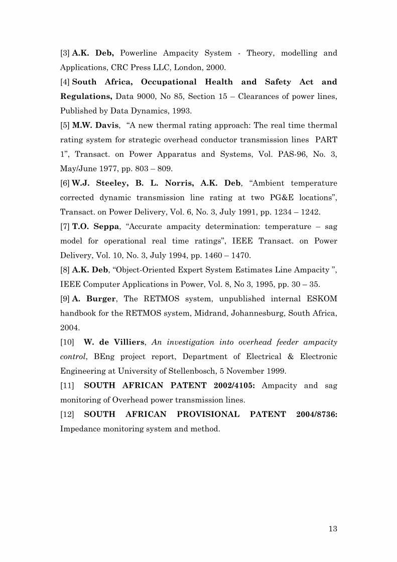
Six main components of the PLC system as shown in Figure 2.1 will now
be described: Overhead Transmission Line (OHTL), Line Trap (LT),
Coupling Capacitor (CC) or Capacitor Voltage Transformer (CVT), Line
Matching Equipment (LME), Phase Combiner (also known as a Hybrid
and is only used for coupling to more than one phase) and the Carrier (a
transceiver).
Station A
LT LT
LME
LME
CC
CCCarrier A
Hybrid
LT LT
Station B
CC
CC
LME
LME
OHTL
Carrier B
Hybrid
Figure 2.1 Simplified PLC system between two Stations
15
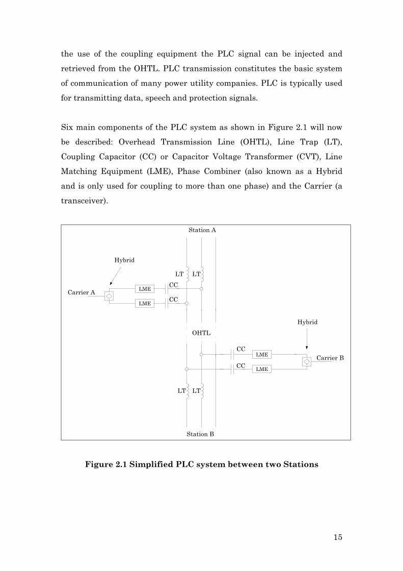
The LT, CC (or CVT) and the LME are located in the High Voltage (HV)
yard of the Station, as indicated by Photograph 2.1. The Carrier and
Hybrid are normally located in the relay room.
LT
CVT
LME
Photograph 2.1 Line Trap (LT), Capacitor Voltage Transformer
(CVT) and Line Matching Equipment (LME)
The main function of each of the six mentioned components in the
framework of the PLC system will now be briefly discussed.
The carrier is the main communication device. All the various types of
signal, for example speech and teleprotection, are transmitted by the local
carrier and received at the remote carrier.
16

The power of the communication signal from the carrier is then split by
the hybrid at the local station to drive the two phases and excite the
desired OHTL natural modes of propagation. The received power at the
remote station is then re-combined via the remote hybrid (Figure 2.1).
The Line Matching Equipment (LME) matches the impedance of the PLC
system to the impedance of the High Voltage OHTL network together with
the other coupling equipment, for maximum signal power transfer to the
OHTL phases.
The low voltage, high frequency carrier signal is then coupled onto the
high voltage OHTL via a Coupling Capacitor (CC) or Capacitive Voltage
Transformer (CVT).
The Line Trap (LT) is a filtering device and is located on the OHTL on the
station side of the CC connection to the OHTL. The LT prevents the
coupled signal from being shorted out in the Station by providing high
impedance in the PLC frequency band. Therefore, the PLC signal energy
is channelled to propagate along the OHTL towards the remote station.
Finally, the OHTL acts like a wave-guide for PLC signals. This can be
seen as part of the transmission path where the PLC signals are guided in
their propagation. The physical dimensions of the line are thus crucial,
because they influence the propagation properties of the coupled signal.
This effect is exploited in this thesis to measure the average height of the
conductors.
The theory of Natural Modes [2], describes OHTL PLC signal propagation
characteristics and will be discussed in the following section.
17

2.3 The theory of natural modes [2][3][4][5]
The attenuation of the PLC signal can be subdivided into two components:
i) The attenuation due to the transmission line, including the
effect of ground resistivity.
ii) The attenuation due to the coupling system.
The latter is relatively simple to compute and is well described, but the
former is more complex. Wedepohl’s “Theory of Natural Modes” [2][3][4][5]
will be introduced to calculate the line attenuation. This is done by first
explaining the eigenvectors and eigenvalues of an OHTL.
2.3.1 Voltage propagation matrix
The impedance and admittance matrixes of a specific OHTL are a function
of the OHTL geometry, the specific conductors configuration used and the
ground resistance. The product of the impedance matrix and the
admittance matrix defines the voltage propagation matrix squared (P), as
shown in Equation 2.1.
[P] ZY= 2.1
The voltage propagation matrix squared can also be expressed (Equation
2.2) by its eigenvalues (λ ) and eigenvectors ( ). vE
1v vP E Eλ −= 2.2
A better understanding of this powerful formulation can be gained if it is
interpreted as follows. The eigenvectors contain the direction of the
vectors or the fixed “physical part” of the solution. The eigenvalues
describe the variable or dynamic characteristics of the solution.
18

A physical interpretation of the eigenvalues (λ ) and eigenvectors ( ) will
be given in terms of the natural modes in a multi-conductor system.
vE
2.3.2 Eigenvectors of the voltage propagation matrix
The modal matrix of the system relates to the eigenvectors and is fixed
because of physical geometry. The modes are called the natural modes of a
multi-conductor system. For a flat configuration transmission line the
‘Clarke vector’ (Equation 2.3) is a very good approximation of the natural
modes.
1 1 12
_ 1 01 1 12
vE Clarke Vector 1
≈ = −
−
2.3
The three Columns of Equation 2.3 describes the natural modes for a flat
OHTL configuration, which are known respectively as the “least
attenuated mode” (Column 1), “the differential mode” (Column 2) and the
“most attenuated mode” (Column 3).
Any voltage matrix coupled to the OHTL will be distributed in its natural
modes and will propagate along the OHTL. The distribution of a coupled
voltage matrix in its natural modes will now be further explained by an
example.
Example: Standard differential coupling between the Outer phase and the
Centre phase at the local station to the Outer phase and Centre phase at
the remote station.
19

Figure 2.2 represents a transmission line with three phases, which
describes a coupling configuration in general terms for a flat transmission
line configuration.
1 2 3
Vp1 Vp2 Vp3
Phase conductors
Ground plane
Figure 2.2 Coupling notation (Vp1,Vp2,Vp3) on a flat configuration
OHTL
The standard coupling configuration (called differential coupling) of a PLC
system which has coupling equipment on two phases (Figure 2.1), can be
expressed as (Equation 2.4):
1
2
3
110
p
a p
p
VV V
V
− = =
2.4
Where
Voltage vector at location or station aVoltage on phase N
a
pN
VV
==
Let Subscript ‘a’ be the position along the transmission line where the
local station is, ‘b’ the position along the transmission line where the
remote station is and ‘x’ any position along the OHTL.
The coupled voltage matrix will distribute in its natural modes as follows
(Equation 2.5):
20

2.5 1 2 3
(1,1) (1, 2) (1,3)(2,1) (2, 2) (2,3)(3,1) (3, 2) (3,3)
v v v
a v v v
v v v
E E EV A E A E A E
E E E
= + +
By substituting Equation 2.3 and Equation 2.4 in Equation 2.5, the
distribution vector ‘A’ can be computed to be:
1
2
3
0.50.5
0
AAA
= −= −=
2.6
To conclude the example, Figure 2.3 shows a graphical representation of
the modal distribution for a signal which was coupled differentially onto
the Outer phase (P1) and Centre phase (P2).
Figure 2.3 Graphical representation of the Modal distribution for
a differentially coupled signal
The total power coupled onto the OHTL via a specific coupling
configuration will distribute between the abovementioned natural modes.
The standard coupling configuration (Equation 2.4) will excite 75% of
mode 1 (least attenuated mode) 25% of mode 2 and 0% of mode 3 on a flat
OHTL as in Figure 2.2.
21

The attenuation characteristics of the modes will be described in the
following section.
2.3.3 Eigenvalues of the voltage propagation matrix
The eigenvalues describe the dynamic characteristics of the different
natural modes (eigenvectors) of the system. Thus, the attenuation and
phase retardation of modes are associated with the eigenvalues.
The attenuation constant (α ) and phase velocity ( β ) can be computed by
taking the square root of the eigenvalue of mode i (Equation 2.7):
i i ij iλ α β γ= + = 2.7
The typical modal attenuations for a flat transmission line are plotted in
Figure 2.4 to provide the reader with a framework for comparison of the
different attenuation constants.
22

Figure 2.4 Typical attenuation constants for the different modes.
(9 m-phase spacing, 19.6 m conductor height, twin dinosaur phase
conductor type and 300 ohm-meter ground resistance)
From Figure 2.4, it is clear why mode 1 is called the least attenuated mode
and mode 3 the most attenuated mode or the ground mode.
2.3.4 Multi-Conductor Wave equation
The voltage propagation matrix squared was defined in Equation 2.2. The
voltage propagation matrix can now be defined as (Equation 2.8)
1v vE Eγ −Γ = 2.8
where
γ λ= (Modal propagation constant)
23

The multi-Conductor wave equation can now be expressed as (Equation
2.9)
2.9 ( ) ( )x xx aV e V e V−Γ Γ= + b
where is the voltage on the transmission line xV 0x = away, V is the
coupled voltage at and V is the reflected wave. For simplicity let us
assume a very long transmission line, which will result in V . Equation
2.9 can then be expressed by its natural modes or eigenvalues as [3]
a
0x = b
0b ≈
2.10 1xx v vV E e E Vγ −−= a
Finally, for a flat transmission line, we can express Equation 2.10 by using
the Clarks vectors (Equation 2.3) and the Voltage distribution as:
1
2
3
1
1
2
3
1 11 1 1 10 02 21 0 1 0 0 1 0 11 0 0 11 1 1 12 2
xp
xx p
xp
e VV e
e V
γ
γ
γ
−
−
−
−
− − = − − − −
V
v k
2.11
Choose a voltage V to be equal to column ‘k’ of the eigenvoltage ( )
vector matrix, thus coupling a particular natural mode. Then Equation
2.11 simplifies to Equation 2.12:
a vE
2.12 ( )k x
xV e Eγ−=
This is a significant result and proves that the sending end voltage
retains its distribution, which is being multiplied by a scalar factor .
This is similar to a transmission line with one propagation constant. It is
for this reason that the various
( )v kE
( )k xγ−e
γ are known as modal propagation
24
constants, the columns of are known as the modal voltage vectors and
the theory is known as the “theory of natural modes” [2].
( )v kE
In the next section the simulation program that was developed at
Stellenbosch University will be discussed, with the emphasis on
developing a model. The specific definitions of the model that relate the
average height of an OHTL conductor to the signal propagation
characteristics of PLC-SAG tones will also be discussed in detail.
2.4 PLC – SAG model development
The goal of the PLC-SAG simulation model is twofold.
The first goal of the model is to perform a sensitivity analysis. It is
important to assess the phenomenon of PLC-SAG tone variation due to
conductor height variations and whether these variations are prominent
enough on the relevant OHTL.
The model is not accurate enough to relate the measured attenuation
directly to conductor height, due to inaccuracies of input parameters (such
as ground resistivity), assumptions and station impedance uncertainties.
An on-site calibration procedure, which will be discussed in Chapter 6,
was developed to achieve the needed accuracy.
The second goal was to identify possible faulty components on the existing
operational PLC system. On short lines components, such as the tuning
unit of a line trap, could be faulty without influencing the system. This is
because the losses in the system are not significant due to the shortness of
the transmission line. The system could thus be fully functional under
normal conditions without the power utility being aware of the faulty
component (or components) except under line fault conditions.
25
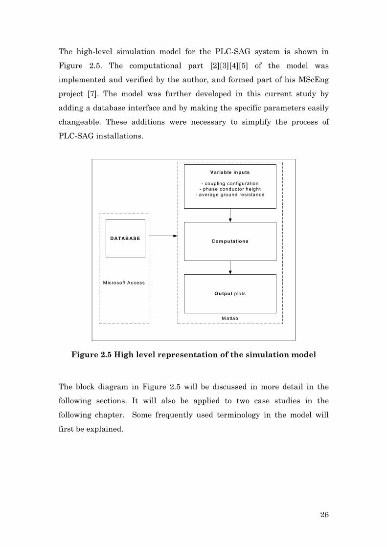
The high-level simulation model for the PLC-SAG system is shown in
Figure 2.5. The computational part [2][3][4][5] of the model was
implemented and verified by the author, and formed part of his MScEng
project [7]. The model was further developed in this current study by
adding a database interface and by making the specific parameters easily
changeable. These additions were necessary to simplify the process of
PLC-SAG installations.
M atlab
M icrosoft Access
Variable inputs
- coup ling configuration- phase conductor height
- average ground resistance
Com putationsD ATAB ASE
O utput p lots
Figure 2.5 High level representation of the simulation model
The block diagram in Figure 2.5 will be discussed in more detail in the
following sections. It will also be applied to two case studies in the
following chapter. Some frequently used terminology in the model will
first be explained.
26
2.4.1 Model definitions
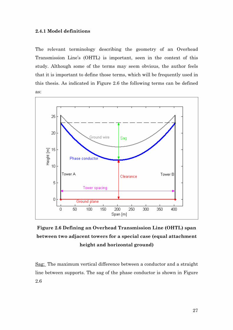
The relevant terminology describing the geometry of an Overhead
Transmission Line’s (OHTL) is important, seen in the context of this
study. Although some of the terms may seem obvious, the author feels
that it is important to define those terms, which will be frequently used in
this thesis. As indicated in Figure 2.6 the following terms can be defined
as:
Figure 2.6 Defining an Overhead Transmission Line (OHTL) span
between two adjacent towers for a special case (equal attachment
height and horizontal ground)
Sag: The maximum vertical difference between a conductor and a straight
line between supports. The sag of the phase conductor is shown in Figure
2.6
27

Clearance: The minimum distance between the phase conductor and the
ground plane. According to the Occupational Health and Safety (OHS) Act
[1] in South Africa the minimum clearance of a 400 kV OHTL is 8.1m. The
minimum distance between the ground plane and the phase conductor is
not necessarily in the middle of the span.
Equivalent Span: Because the PLC-SAG method measures the average
height variation of the whole transmission line, the transmission line will
be described in terms of its equivalent span. The equivalent span is the
span that represents all the individual spans of the transmission line.
Some textbooks also refer to it as the ruling span. In the context of this
thesis the two parameters that describe the equivalent span are the tower
spacing and the attachment height.
The tower spacing of the equivalent span (Le) is defined as [9]:
3 3 3 31 2 3
1 2 3
......
ne
n
L L L LLL L L L
+ + + +=
+ + + + 2.13
where
e
i
L = equivalent spanL = tower spacing of each individual span n = total number of spans
The attachment heights of the phase conductor and the ground wire, for
the equivalent span, can be computed by analysing the tower dimensions.
Average conductor height: One of the assumptions of the model is that it
uses the average conductor height to do simulations. The average
conductor height is, as the name indicates, the average height of the
conductor of the equivalent span above a flat horizontal ground plane.
28

0
1 ( )eL
avee
h h xL
= ∫ dx (2.14)
where
Le = Length of the span as shown in Figure 2.7.
Figure 2.7 Average conductor height
The average ground wire height is defined in a similar manner.
Default Simulation Condition: The average heights of the Equivalent span
of the phase conductor and ground wire, when tensioned to have a
catenary constant [9] of 2100 m and 1800 m respectively. These values of
the catenary constant are adopted from an in-house rule1 in ESKOM (the
main power utility in South Africa).
1 Personal communication with Mr P Marais, Head Structural Engineer of
TAP (Trans-Africa Projects, a division of ESKOM) dated 2004/07/13
29
With the definitions cleared, the high level model will be discussed in two
sections; the database (Left-hand side of Figure 2.5) and the Matlab
simulations options (middle of Figure 2.5)
2.4.2 Database (Microsoft Access, left-hand side of Figure 2.5)
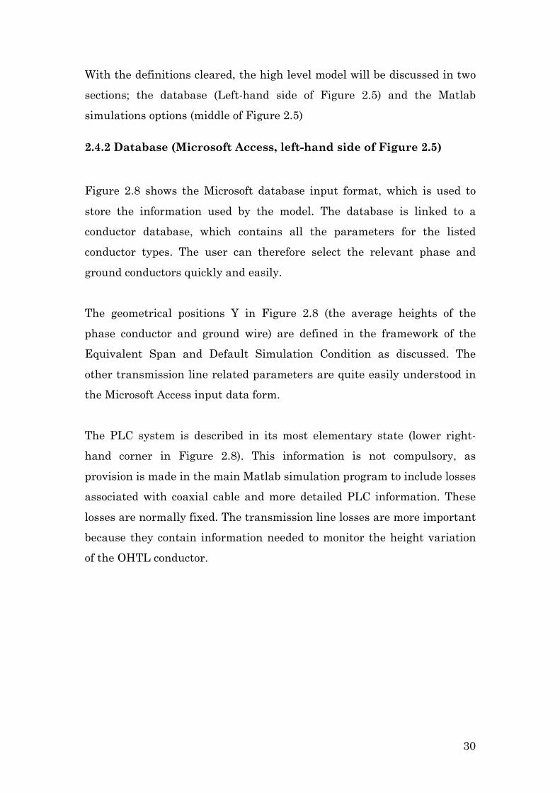
Figure 2.8 shows the Microsoft database input format, which is used to
store the information used by the model. The database is linked to a
conductor database, which contains all the parameters for the listed
conductor types. The user can therefore select the relevant phase and
ground conductors quickly and easily.
The geometrical positions Y in Figure 2.8 (the average heights of the
phase conductor and ground wire) are defined in the framework of the
Equivalent Span and Default Simulation Condition as discussed. The
other transmission line related parameters are quite easily understood in
the Microsoft Access input data form.
The PLC system is described in its most elementary state (lower right-
hand corner in Figure 2.8). This information is not compulsory, as
provision is made in the main Matlab simulation program to include losses
associated with coaxial cable and more detailed PLC information. These
losses are normally fixed. The transmission line losses are more important
because they contain information needed to monitor the height variation
of the OHTL conductor.
30
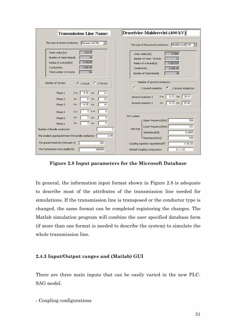
Figure 2.8 Input parameters for the Microsoft Database
In general, the information input format shown in Figure 2.8 is adequate
to describe most of the attributes of the transmission line needed for
simulations. If the transmission line is transposed or the conductor type is
changed, the same format can be completed registering the changes. The
Matlab simulation program will combine the user specified database form
(if more than one format is needed to describe the system) to simulate the
whole transmission line.
2.4.3 Input/Output ranges and (Matlab) GUI
There are three main inputs that can be easily varied in the new PLC-
SAG model.
- Coupling configurations
31
- Conductor height variation
- Ground resistivity
The output of the simulation is the required attenuation for PLC
frequencies (50 kHz – 500 kHz). This is represented in a graphical format
(simulations are performed in the following chapter) but is also saved in a
matrix format for extended data processing.
The three input parameters will now be discussed, followed by the
Graphical User Interface (GUI).
Different coupling configurations
The standard coupling configuration (called differential coupling) for a
PLC system, which has coupling equipment on two phases, can be
expressed as Equation 2.4.
If the transmission line is not transposed then the same coupling
configuration is used to decouple signals from the transmission line. This
coupling configuration relates to the specific installation shown in Figure
2.1. Coupling equipment is installed on two of the phases. The hybrid in
Figure 2.1 not only divides the PLC signal into two paths, but also
introduces a 180-degree phase shift, thus the sign difference between Vp1
and Vp2. The decoupling vector at the remote station would be the same
as the coupling vector shown in Equation 2.4.
From Section 2.3 it is evident that different propagation modes are
energized in different ratios, dependent on the initial coupling
configuration. The standard differential coupling configuration is chosen
to ensure robust operation for the PLC system. However, the attenuation
variation of a PLC signal coupled in this way is not very sensitive for
determining the height of the conductor as may be expected.
32
Phase conductor height variation
For each coupling configuration the average phase conductor height must
be varied to identify the “best” coupling configuration, with “best” meaning
the coupling arrangement which is most sensitive to average height
variations.
From previous simulations [7] it is evident that height variation of the
ground wire does not influence the PLC-SAG tone attenuation
significantly for a flat transmission line configuration. Therefore the
height of the earth wire can be kept fixed during the simulations.
Ground resistance
The quality of the simulations is limited to the accuracy of the input
parameters. One of the most difficult input parameters to estimate is the
average ground resistance. A new technique to improve the estimation of
the ground resistance has been developed and will be discussed in a
subsequent section.
GUI (Graphical User Interface)
All the above-mentioned parameters can easily be changed for exploration
simulations. A snapshot of the simulation program output is shown in
Figure 2.9. Before the additions were made it was very cumbersome and
time consuming to perform a range of simulations (Chapter 3). The GUI
was also developed in Matlab. As mentioned before, the results of the
simulation program are also saved in a file. This feature was very useful
in a research environment. For example, the simulation data in the file
can be incorporated together with measured values to perform
comparisons in another program.
33
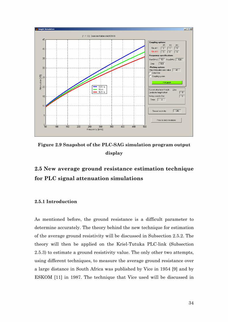
Figure 2.9 Snapshot of the PLC-SAG simulation program output
display
2.5 New average ground resistance estimation technique
for PLC signal attenuation simulations
2.5.1 Introduction
As mentioned before, the ground resistance is a difficult parameter to
determine accurately. The theory behind the new technique for estimation
of the average ground resistivity will be discussed in Subsection 2.5.2. The
theory will then be applied on the Kriel-Tutuka PLC-link (Subsection
2.5.3) to estimate a ground resistivity value. The only other two attempts,
using different techniques, to measure the average ground resistance over
a large distance in South Africa was published by Vice in 1954 [9] and by
ESKOM [11] in 1987. The technique that Vice used will be discussed in
34
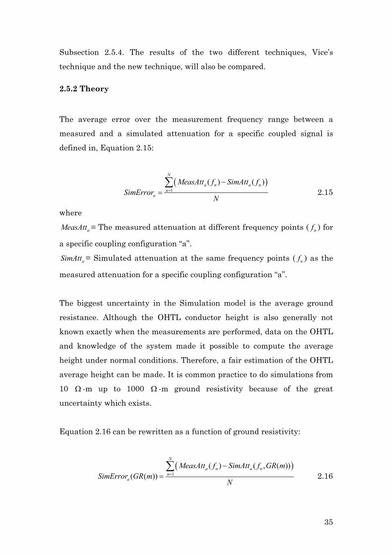
Subsection 2.5.4. The results of the two different techniques, Vice’s
technique and the new technique, will also be compared.
2.5.2 Theory
The average error over the measurement frequency range between a
measured and a simulated attenuation for a specific coupled signal is
defined in, Equation 2.15:
( )
1( ) ( )
N
a n a nn
a
MeasAtt f SimAtt fSimError
N=
−=
∑ 2.15
where
aMeasAtt = The measured attenuation at different frequency points ( nf ) for
a specific coupling configuration “a”.
aSimAtt = Simulated attenuation at the same frequency points ( nf ) as the
measured attenuation for a specific coupling configuration “a”.
The biggest uncertainty in the Simulation model is the average ground
resistance. Although the OHTL conductor height is also generally not
known exactly when the measurements are performed, data on the OHTL
and knowledge of the system made it possible to compute the average
height under normal conditions. Therefore, a fair estimation of the OHTL
average height can be made. It is common practice to do simulations from
10 -m up to 1000 -m ground resistivity because of the great
uncertainty which exists.
Ω Ω
Equation 2.16 can be rewritten as a function of ground resistivity:
( )
1( ) ( , ( ))
( ( ))
N
a n a nn
a
MeasAtt f SimAtt f GR mSimError GR m
N=
−=
∑ 2.16
35

where:
( ) 10,...,1000 m for m = 1,....,M GR m = Ω −
A range of simulations can then be performed to search for the ground
resistivity (GR), which will minimize the error in Equation 2.16. Assuming
that there are no faults in the PLC system, the danger in this approach is
that changing the ground resistivity (GR) could mask another error in the
simulation program. To minimize this possibility, the same process can be
repeated for the different coupling configurations that produce a unique
attenuation response. This means that propagation modes are energized
in different ratios, which would result in different attenuations (Section
2.3). Let us assume five different unique coupling configurations (“a” to
“e”), which can be practically measured on a PLC system. The best ground
resistivity can then be identified as the ground resistivity, which produces
the minimum error between the measurements and the simulations:
2.17
( ) ( ( ))
then( ) such that C(m) C(n) where n m
e
couplingcoupling a
best
C m SimError GR m
GR GR m
=
=
= ≤
∑
≠
The following section will test this technique in practice as it was applied
on the Kriel-Tutuka OHTL.
2.5.3 Simulations and average ground resistivity for the PLC link
between Kriel power station and Tutuka power station.
The technique comprises 4 steps:
1) Identify the practical number of unique coupling configurations for
the specific PLC system
2) Simulate the relevant attenuation for a spectrum of ground
resistivity values (More details about the line and simulation
process is given in Chapter 3)
36
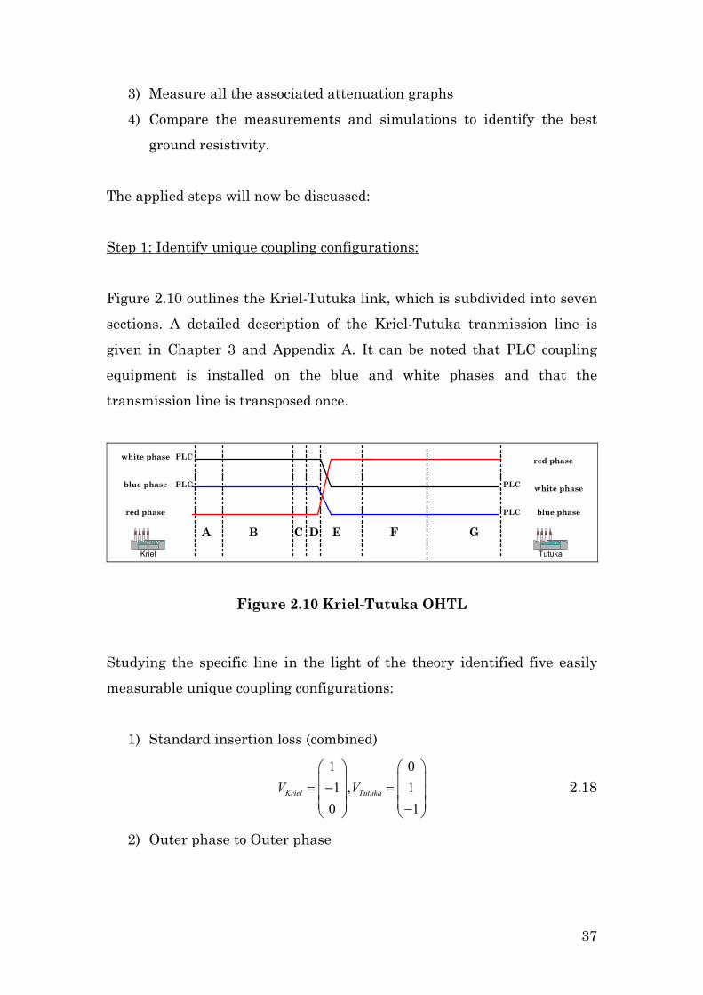
3) Measure all the associated attenuation graphs
4) Compare the measurements and simulations to identify the best
ground resistivity.
The applied steps will now be discussed:
Step 1: Identify unique coupling configurations:
Figure 2.10 outlines the Kriel-Tutuka link, which is subdivided into seven
sections. A detailed description of the Kriel-Tutuka tranmission line is
given in Chapter 3 and Appendix A. It can be noted that PLC coupling
equipment is installed on the blue and white phases and that the
transmission line is transposed once.
Kriel Tutuka
A B C D E F
white phase
blue phase
red phase
PLC
PLC PLC
PLC
white phase
blue phase
red phase
G
Figure 2.10 Kriel-Tutuka OHTL
Studying the specific line in the light of the theory identified five easily
measurable unique coupling configurations:
1) Standard insertion loss (combined)
1 01 , 1
0 1Kriel TutukaV V
= − = −
2.18
2) Outer phase to Outer phase
37

2.19 1 00 , 00 1
Kriel TutukaV V = =
3) Centre phase to Centre phase
2.20 0 01 , 10 0
Kriel TutukaV V = =
4) Centre phase to Outer phase
2.21 0 01 , 00 1
Kriel TutukaV V = =
5) Outer phase to Centre phase
2.22 1 00 , 10 0
Kriel TutukaV V = =
Step 2: Simulations
With all the detailed information of the OHTL (Appendix A) the signal
attenuation can be simulated for the different coupling configurations and
the spectrum of ground resistances. The average height of the conductor
is calculated for the default simulation condition as explained in Section
2.4.1. Figure 2.11 shows the attenuation for the five different coupling
configurations for a ground resistance of 50 mΩ − .
38
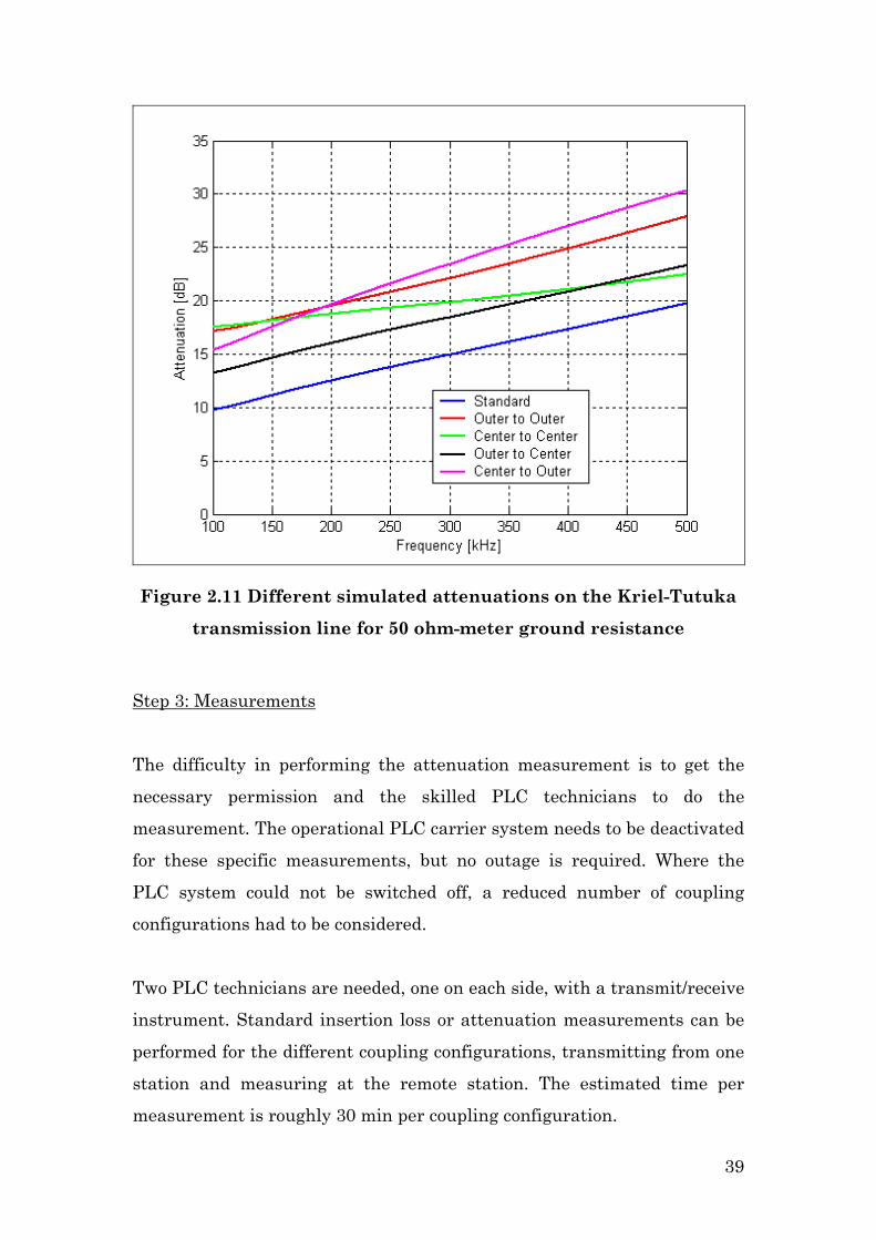
Figure 2.11 Different simulated attenuations on the Kriel-Tutuka
transmission line for 50 ohm-meter ground resistance
Step 3: Measurements
The difficulty in performing the attenuation measurement is to get the
necessary permission and the skilled PLC technicians to do the
measurement. The operational PLC carrier system needs to be deactivated
for these specific measurements, but no outage is required. Where the
PLC system could not be switched off, a reduced number of coupling
configurations had to be considered.
Two PLC technicians are needed, one on each side, with a transmit/receive
instrument. Standard insertion loss or attenuation measurements can be
performed for the different coupling configurations, transmitting from one
station and measuring at the remote station. The estimated time per
measurement is roughly 30 min per coupling configuration.
39

The measurement results of all the different coupling configurations will
be presented in the following section.
Step 4: Comparison and identification of the best ground resistance value
This step is started by doing simulations from 10 Ω -m to 1000 Ω -m.
Table 2.1 shows the errors as defined in Equation 2.17. The least average
error (Equation 2.18) and the associated resistance are presented in bold
type in the table. Only resistivity values from 50 mΩ − to 100 are
shown in Table 2.1.
mΩ −
Table 2.1 Ground resistivity errors for differed coupling
configurations
Ground resistivity (ohm-metre) 50 60 70 80 90 100
Standard configuration 2.199641 1.920269 1.681415 1.474366 1.321156 1.152466
Outer phase to Outer phase 1.515003 1.443741 1.400946 1.488166 1.68877 2.041184
Centre phase to Centre phase 4.038622 4.032896 4.033539 4.038473 4.046318 4.226727
Outer phase to Centre phase 2.367882 2.094308 1.860129 1.662253 1.492668 1.249736
Centre phase to Outer phase 1.654107 1.576879 1.633531 1.820509 2.167821 2.760368
Average error 2.355051 2.213619 2.121912 2.096754 2.143347 2.286096
The measurement and the simulations are shown in Figure 2.12 to Figure
2.16 for an average ground resistivity of 80 mΩ − .
40

100 150 200 250 300 350 400 450 5000
5
10
15
20
25
30
35
Frequency [kHz]
Atte
nuat
ion
[dB
]
SimulationMeasurement
Figure 2.12 Measurement and simulation for standard coupling
configurations (Equation 2.19)
100 150 200 250 300 350 400 450 5000
5
10
15
20
25
30
35
Frequency [kHz]
Atte
nuat
ion
[dB
]
SimulationMeasurement
Figure 2.13 Measurement and simulation for outer phase to outer
phase (Equation 2.20)
41

100 150 200 250 300 350 400 450 5000
5
10
15
20
25
30
35
Frequency [kHz]
Atte
nuat
ion
[dB
]
Center to Center
SimulationMeasurement
Figure 2.14 Measurement and simulation for centre phase to
centre phase (Equation 2.20)
100 150 200 250 300 350 400 450 5000
5
10
15
20
25
30
35
Frequency [kHz]
Atte
nuat
ion
[dB
]
Outer to Center
SimulationMeasurement
Figure 2.15 Measurement and simulation for outer phase to centre
phase (Equation 2.21)
42

100 150 200 250 300 350 400 450 5000
5
10
15
20
25
30
35
Frequency [kHz]
Atte
nuat
ion
[dB
]
SimulationMeasurement
Figure 2.16 Measurement and simulation for centre phase to outer
phase (Equation 2.22)
This is a remarkably good result, measured and simulated for a
transposed transmission line that consists of seven different sections. The
centre phase to centre phase simulation indicates the biggest average
error of 4.04 dB and the standard coupling configuration the smallest
error of 1.47 dB. The biggest error could be due to the station impedance
uncertainty.
2.5.4 Comparing the technique with other techniques
The only other attempt to determine the average ground resistance over a
long distance at PLC frequencies in South Africa was done by R.W. Vice
between 1950 and 1952 [9]. From this survey, a ground conductivity map
of South Africa was created. The ground resistance was determined by
43
analysing its effect on ground wave propagation between two distant
antennas. According to the survey, the area in the vicinity of the location
of the Kriel-Tutuka transmission line has an average ground resistance
between 50 and 58 Ω − . This compares well with the determined 80
via the PLC technique, when considered in the framework of the
wide range (10 Ω to 1000
m
/ m
/ mΩ
/ mΩ ) of the ground resistance. An
important difference between the two techniques is that Vice [9]
determined the ground’s resistance only at 500 kHz, whereas the PLC
technique is applied over the PLC frequency range (100 kHz – 500 kHz).
2.6 Conclusion
Some background about the PLC system and the associated theory of
natural modes is given. The eigenvector and eigenvalues are described in
the context of signal propagation on an OHTL.
Terms used in the PLC-SAG model, which will be used consistently
throughout the thesis, are discussed. Additional changes were made to the
simulation program as described in [7], to ensure that it was tailor made
for PLC-SAG related simulations.
A PLC technique to estimate the average ground resistance was created.
This is a new contribution to the simulation model and was successfully
done and evaluated.
References:
[1] D.C. Smith, PLC system engineering and practical application,
unpublished notes, for one-day short course, University Stellenbosch,
1999.
44

[2] L.M. Wedepohl, The Theory of Natural Modes in Multi-Conductor
Transmission Systems, unpublished lecture notes, Westbank, British
Columbia, Canada, 10 January 1999.
[3] Wedepohl, L.M. “Applecation of Matrix Methods to the Solution of
Travelling Wave Phenomena in Polyphase Systems”, Proc. IEE, Vol. 110,
Dec. 1963, p. 2200-2212. (13 Pages)
[4] Galloway, R.H., Shorrocks, W.B., Wedepohl, L.M. “Calculations of
Electrical Parameters for Short and Long Polyphase Transmission Lines”,
Proc. IEE, Vol. 111, No. 12, Dec.1964, p. 2051-2059. (9 pages)
[5] Wedepohl, L.M. “Electrical Characteristics of Polyphase
Transmission System, With Special Reference to Boundary Value
Calculations at Power Line Carrier Frequencies”, Proc. IEE, Vol. 112, No.
11, Nov. 1965, p.2103-2112. (10 pages)
[6] F.Eggimann, W.Senn and K. Morf, “The Transmission
Characteristics of High-Voltage Lines at Carrier Frequencies”, Brown
Boveri Review 8-77, pp. 449-459.
[7] De Villiers, W., Prediction and measurement of Power Line Carrier
signal attenuation and fluctuation, MScEng Thesis, University of
Stellenbosch, November 2001.
[8] Occupational Health and Safety Act of South Africa, Section 15:
Clearances of power lines, 1993.
[9] Turan Gönen, Electric power transmission system engineering –
Analysis and Design, John Wiley and Sons, New York, 1988.
[10] R.W. Vice, “A survey of ground wave propagation conditions in
South Africa”, The Transactions of the S.A. Institute of Electrical
Engineers, April 1954, pp. 139-159
[11] A.F. Pollard, “Power Line Carrier and teleportation Design for
Eskom’s 765 kV system”, ESKOM open Conference on EHV transmission
systems, MegaWatt Park in South Aftrica, 23 Nov 1987.
45

Chapter 3
Simulation of the two case studies and
frequency allocation of the PLC-SAG
monitoring tones
3.1 Introduction
The two case studies of two transmission lines on which the PLC-SAG
experimental systems were installed will be introduced. Simulations will
be performed on the case studies and frequencies will be allocated for the
PLC-SAG monitoring tones.
The first case study on which the PLC-SAG experiment was installed was
the 400 kV transmission line between Koeberg Power Station and Acacia
Sub Station, which is located in the Western Cape and is 31.318 km long.
This line is considered a typical OHTL.
The second case study was done on the 400 kV transmission line between
Kriel Power Station and Tutuka Power Station. This line is located in
Mpumalanga and is 99.17 km long. The line is transposed once and has
seven different sections due to previous changes made to the OHTL. This
line is not classified as a typical OHTL and was chosen as an extreme
case, in order to test the PLC-SAG system.
In this thesis the abbreviation ‘KA’ will be used to refer to the 400 kV
transmission line between Koeberg Power Station and Acacia Sub Station
46
and ‘KT’ will be used when referring to the 400 kV transmission line
between Kriel Power Station and Tutuka Power Station.
After more detail on the two case studies has been introduced in Section
3.2, simulations will be performed in Section 3.3 using the simulation
program as described in the previous chapter. The PLC signal attenuation
will be simulated for different coupling configurations and at different
conductor heights above the ground. Five different coupling configurations
were explored, from which the best coupling configuration was selected.
To explore the expected PLC signal level variations (simulated in this
chapter) as a function of conductor height, a multi-tone experiment was
proposed on each of the two case studies. After consultation with ESKOM
it was concluded that 10 tones could be coupled and decoupled on each of
the lines in the case studies. The frequency allocation process of the ten
tones will be discussed in this chapter (Section 3.4), as it relates closely to
the simulations presented. In Chapter 4 the physical hardware
implementation of the experiment will be discussed.
3.2 Locations of the two OHTL sites
3.2.1 General
Two OHTLs in South Africa were chosen on which to install PLC-SAG
systems. The most important criterion for an OHTL to be a candidate for
PLC-SAG Ampacity control is that it should have an operational PLC
system installed.
The KA line was chosen because it was a short (31.318 km), non-
transposed flat horizontal OHTL and conveniently close to Stellenbosch
University. The second transmission line had to be selected with more
47
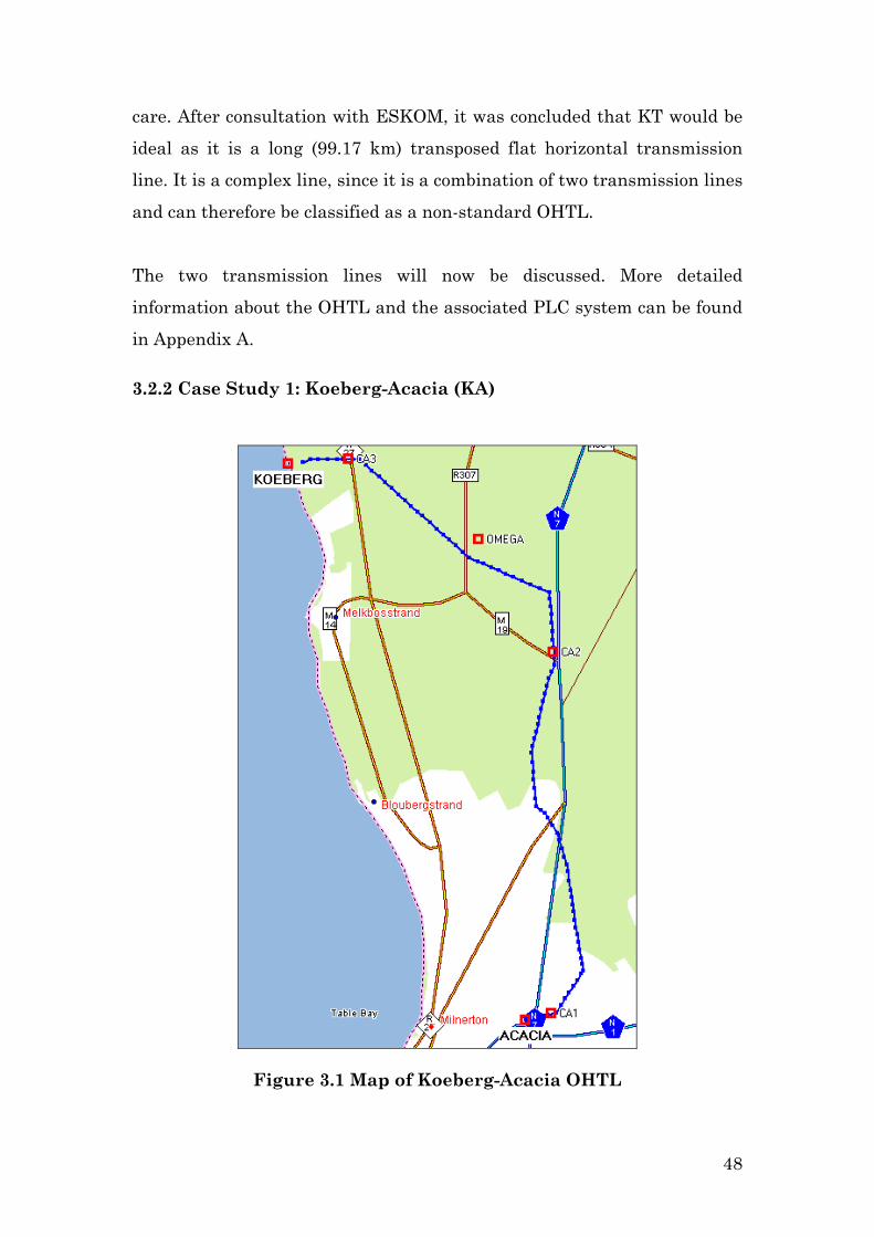
care. After consultation with ESKOM, it was concluded that KT would be
ideal as it is a long (99.17 km) transposed flat horizontal transmission
line. It is a complex line, since it is a combination of two transmission lines
and can therefore be classified as a non-standard OHTL.
The two transmission lines will now be discussed. More detailed
information about the OHTL and the associated PLC system can be found
in Appendix A.
3.2.2 Case Study 1: Koeberg-Acacia (KA)
Figure 3.1 Map of Koeberg-Acacia OHTL
48
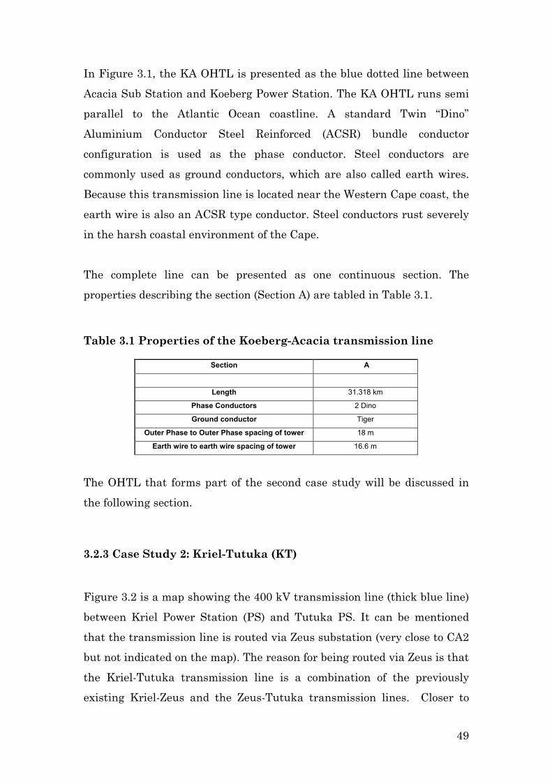
In Figure 3.1, the KA OHTL is presented as the blue dotted line between
Acacia Sub Station and Koeberg Power Station. The KA OHTL runs semi
parallel to the Atlantic Ocean coastline. A standard Twin “Dino”
Aluminium Conductor Steel Reinforced (ACSR) bundle conductor
configuration is used as the phase conductor. Steel conductors are
commonly used as ground conductors, which are also called earth wires.
Because this transmission line is located near the Western Cape coast, the
earth wire is also an ACSR type conductor. Steel conductors rust severely
in the harsh coastal environment of the Cape.
The complete line can be presented as one continuous section. The
properties describing the section (Section A) are tabled in Table 3.1.
Table 3.1 Properties of the Koeberg-Acacia transmission line
Section A
Length 31.318 km
Phase Conductors 2 Dino
Ground conductor Tiger
Outer Phase to Outer Phase spacing of tower 18 m
Earth wire to earth wire spacing of tower 16.6 m
The OHTL that forms part of the second case study will be discussed in
the following section.
3.2.3 Case Study 2: Kriel-Tutuka (KT)
Figure 3.2 is a map showing the 400 kV transmission line (thick blue line)
between Kriel Power Station (PS) and Tutuka PS. It can be mentioned
that the transmission line is routed via Zeus substation (very close to CA2
but not indicated on the map). The reason for being routed via Zeus is that
the Kriel-Tutuka transmission line is a combination of the previously
existing Kriel-Zeus and the Zeus-Tutuka transmission lines. Closer to
49

Tutuka PS one can note another sharp bend in the route of the
transmission line. This is due to the surrounding underground coal mines.
Figure 3.2 Map of Kriel-Tutuka OHTL
.
As a result of the combination of the lines and of changes made over the
years, the KT OHTL is quite complex and can best be described by
dividing the line up into seven sections (Figure 3.3). The key properties of
these sections are given in Table 3.2.
50
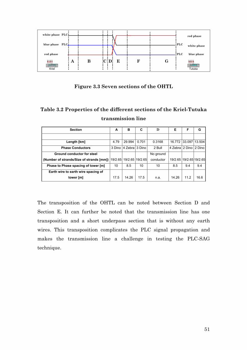
Kriel Tutuka
A B C D E F
white phase
blue phase
red phase
PLC
PLC PLC
PLC
white phase
blue phase
red phase
G
Figure 3.3 Seven sections of the OHTL
Table 3.2 Properties of the different sections of the Kriel-Tutuka
transmission line
Section A B C D E F G
Length [km] 4.79 29.994 0.701 0.3168 16.772 33.097 13.504
Phase Conductors 3 Dino 4 Zebra 3 Dino 2 Bull 4 Zebra 2 Dino 2 Dino
Ground conductor for steel (Number of strands/Size of strands [mm]) 19/2.65 19/2.65 19/2.65
No ground
conductor 19/2.65 19/2.65 19/2.65
Phase to Phase spacing of tower [m] 10 8.5 10 10 8.5 9.4 9.4
Earth wire to earth wire spacing of tower [m] 17.5 14.26 17.5 n.a. 14.26 11.2 16.6
The transposition of the OHTL can be noted between Section D and
Section E. It can further be noted that the transmission line has one
transposition and a short underpass section that is without any earth
wires. This transposition complicates the PLC signal propagation and
makes the transmission line a challenge in testing the PLC-SAG
technique.
51

3.3 Simulations
3.3.1 General
The simulation program and associated theory used are discussed in the
previous chapter. In this section the simulation program is applied to the
two case studies. The simulation methodology will be discussed step by
step.
The first step is to compute the ruling span of the transmission line, in
order to define the default simulation condition (Chapter 2.4.1). Once this
has been accomplished the phase conductor sag can be moved higher and
lower around the default sag value and the associated average conductor
height can be calculated. It is recommended that a lookup table be created
which indicates the relationship between sag and the average conductor
height for the ruling span.
The second step is to perform PLC-SAG tone attenuation simulations for
two scenarios, namely: i) the default simulation condition and ii) a
simulation condition where the phase conductor has sagged two meters
below the default conditions. These simulations can be done for different
coupling configurations, as explained in Chapter 2. The simulations will
indicate which coupling configuration is sensitive to conductor height
variation and show the uniformity of the change in the frequency band.
The final simulation step is to focus on the best coupling configuration as
identified in the previous step and then to change the conductor height in
smaller steps.
These three steps will now be applied to the two different case studies.
52

3.3.2 Case 1: Koeberg-Acacia
Step 1: Calculating the default simulation condition
The attachment height of the phase conductor is a function of the type of
tower used for the transmission line. The attachment height of the
conductor is 19.6 m for the KA OHTL2. The attachment height of the earth
wire can then, in turn, be computed by further studying the tower
dimensions used on this specific OHTL. The vertical spacing between the
phase conductor and the earth wire is 5.55 m and therefore the
attachment height for the earth wire is 25.15 m.
The tower spacing of the equivalent, or ruling span, can be computed by
using Equation 2.13 in Chapter 2. Column seven in Table A.1 of Appendix
A provides the individual lengths ( ) needed. The tower spacing of the
ruling span for KA was calculated as 347.36 m.
eL
0 50 100 150 200 250 300 350
0
5
10
15
20
25
Span [m ]
Hei
ght [
m]
Figure 3.4 Ruling span of Koeberg-Acacia OHTL (Table 3.3)
2 Email correspondence with Mr DC Smith, ESKOM Corporate
Consultant: Telecommunications, dated 1 March 2001
53
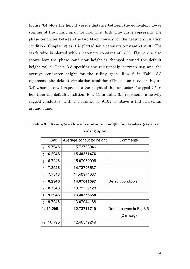
Figure 3.4 plots the height versus distance between the equivalent tower
spacing of the ruling span for KA. The thick blue curve represents the
phase conductor between the two black ‘towers’ for the default simulation
condition (Chapter 2) as it is plotted for a catenary constant of 2100. The
earth wire is plotted with a catenary constant of 1800. Figure 3.4 also
shows how the phase conductor height is changed around the default
height value. Table 3.3 specifies the relationship between sag and the
average conductor height for the ruling span. Row 6 in Table 3.3
represents the default simulation condition (Thick blue curve in Figure
3.4) whereas row 1 represents the height of the conductor if sagged 2.5 m
less than the default condition. Row 11 in Table 3.3 represents a heavily
sagged conductor, with a clearance of 9.105 m above a flat horizontal
ground plane.
Table 3.3 Average value of conductor height for Koeberg-Acacia
ruling span
Sag Average conductor height Comments
1 5.7946 15.73703946
2 6.2946 15.40371476
3 6.7946 15.07039006
4 7.2946 14.73706537
5 7.7946 14.40374067
6 8.2946 14.07041597 Default condition
7 8.7946 13.73709128
8 9.2946 13.40376658
9 9.7946 13.07044188 10 10.295 12.73711719 Dotted curves in Fig 3.5
(2 m sag)
11 10.795 12.40379249
54
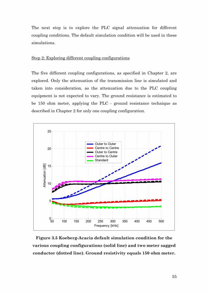
The next step is to explore the PLC signal attenuation for different
coupling conditions. The default simulation condition will be used in these
simulations.
Step 2: Exploring different coupling configurations
The five different coupling configurations, as specified in Chapter 2, are
explored. Only the attenuation of the transmission line is simulated and
taken into consideration, as the attenuation due to the PLC coupling
equipment is not expected to vary. The ground resistance is estimated to
be 150 ohm meter, applying the PLC - ground resistance technique as
described in Chapter 2 for only one coupling configuration.
50 100 150 200 250 300 350 400 450 5000
5
10
15
20
25
Frequency [kHz]
Atte
nuat
ion
[dB
]
Outer to OuterCentre to CentreOuter to CentreCentre to OuterStandard
Figure 3.5 Koeberg-Acacia default simulation condition for the
various coupling configurations (solid line) and two meter sagged
conductor (dotted line). Ground resistivity equals 150 ohm meter.
55
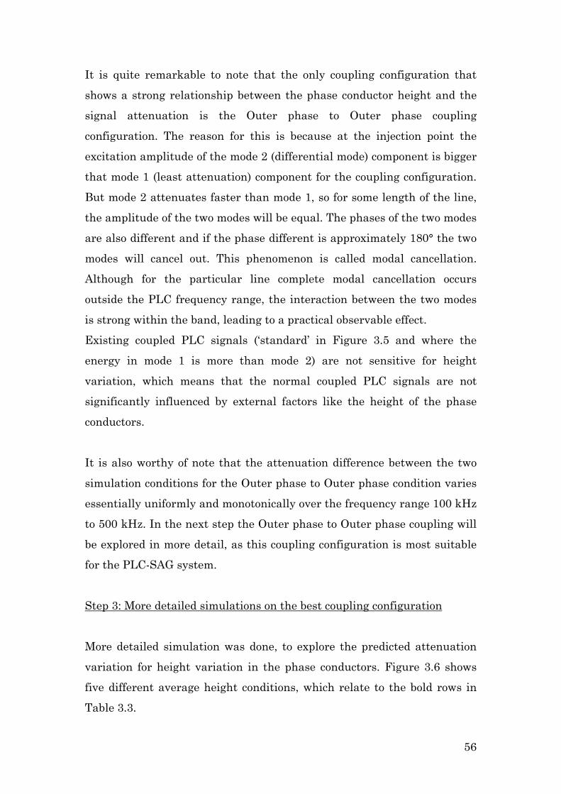
It is quite remarkable to note that the only coupling configuration that
shows a strong relationship between the phase conductor height and the
signal attenuation is the Outer phase to Outer phase coupling
configuration. The reason for this is because at the injection point the
excitation amplitude of the mode 2 (differential mode) component is bigger
that mode 1 (least attenuation) component for the coupling configuration.
But mode 2 attenuates faster than mode 1, so for some length of the line,
the amplitude of the two modes will be equal. The phases of the two modes
are also different and if the phase different is approximately 180° the two
modes will cancel out. This phenomenon is called modal cancellation.
Although for the particular line complete modal cancellation occurs
outside the PLC frequency range, the interaction between the two modes
is strong within the band, leading to a practical observable effect.
Existing coupled PLC signals (‘standard’ in Figure 3.5 and where the
energy in mode 1 is more than mode 2) are not sensitive for height
variation, which means that the normal coupled PLC signals are not
significantly influenced by external factors like the height of the phase
conductors.
It is also worthy of note that the attenuation difference between the two
simulation conditions for the Outer phase to Outer phase condition varies
essentially uniformly and monotonically over the frequency range 100 kHz
to 500 kHz. In the next step the Outer phase to Outer phase coupling will
be explored in more detail, as this coupling configuration is most suitable
for the PLC-SAG system.
Step 3: More detailed simulations on the best coupling configuration
More detailed simulation was done, to explore the predicted attenuation
variation for height variation in the phase conductors. Figure 3.6 shows
five different average height conditions, which relate to the bold rows in
Table 3.3.
56

50 100 150 200 250 300 350 400 450 5000
5
10
15
20
25
Frequency [kHz]
Atte
nuat
ion
[dB
]
12.7m13.414m14.7m15.4m
Figure 3.6 Expected PLC-SAG tone variation with average height
for Outer phase to Outer phase coupling on Koeberg-Acacia OHTL
In Figure 3.6 it can be noted that the attenuation variation range
increases as the frequency increases. A total variation of 5 dB can be noted
at 350 kHz for an average conductor height variation of 2.7m. More
detailed discussions about the mathematical relationship between
attenuation and average conductor height will be given in Chapter 6.
The same three simulation steps will now be applied to the KT OHTL.
3.3.3 Case Study 2: Kriel-Tutuka
Step 1: Calculating the default simulation condition
Figure 3.7 shows the ruling span (404 m) and the attachment height
(Phase conductor = 23 m and earth wire = 25.4 m). The information
needed for these calculations is shown in Appendix A. A clear difference
57
can be noted in the attachment height of the earth wire compared to the
KA case. This is due to the different type of OHTL tower used. As in the
previous simulations, the thick blue line represents the default simulation
condition as defined in Chapter 2. Table 3.4 shows the relationships
between the average conductor height and the sag of the KT ruling span.
0 50 100 150 200 250 300 350 400
0
5
10
15
20
25
Span [m]
Hei
ght [
m]
Figure 3.7 Ruling span of Kriel-Tutuka transmission line
58

Table 3.4 Average value of conductor height for the Kriel-Tutuka
ruling span
Sag
Average conductor
height Comments
1 8.7 17.2
2 9.2 16.9
3 9.7 16.5
4 10.2 16.2
5 10.7 15.9
6 11.2 15.5 Default condition
7 11.7 15.2
8 12.2 14.9
9 12.7 14.5
10 13.2 14.2 Dotted curves in Fig 3.8
11 13.7 13.9
Step 2: Exploring different coupling configurations
The results of the different coupling configurations in Figure 3.8 for KT
OHTL differ greatly from similar simulations for KA OHTL. The main
reason for the difference is that all the configurations indicate some
dependence on average conductor height, which fact is due to the
transposition in the KT line.
59

50 100 150 200 250 300 350 400 450 5000
5
10
15
20
25
30
Frequency [kHz]
Atte
nuat
ion
[dB
]Outer to OuterCentre to CentreStandardOuter to CentreCentre to Outer
Figure 3.8 Default simulation condition for the various coupling
configurations (solid line) and conductor sagged by two meters
(dotted line)
However, the Outer phase to Outer phase coupling configuration again
performed well as regards conductor height sensitivity and uniform
variation throughout the frequency range. A more or less uniform
variation is necessary in order to relate multi coupled PLC-SAG tones to
each other.
Step 3: More detailed simulations on the best coupling configuration
Average conductor height simulations were done, which relate to the bold
rows from Table 3.4. These simulations are shown in Figure 3.9.
60

50 100 150 200 250 300 350 400 450 500
10
12
14
16
18
20
22
24
26
28
30
Frequency [kHz]
Atte
nuat
ion
[dB
]
14.15m14.82515.5m16.175m16.85m
Figure 3.9 Expected PLC-SAG tone variation with average height
for Outer phase (white phase at Kriel, Figure 2.9) to Outer phase
(blue phase at Tutuka) coupling on Kriel-Tutuka OHTL
The sensitivity of the long, transposed KT OHTL was, surprisingly, very
similar to that of the short non-transposed KA OHTL.
Thus the simulation predicted that for both case studies OHTLs had the
necessary PLC-SAG sensitivity, if the PLC-SAG tones were coupled and
decoupled on the Outer phases only. The following section will focus on the
process of allocating PLC-SAG tone frequencies, in order to explore and
verify the expected variations as simulated.
61

3.4 Choosing PLC-SAG tones
3.4.1 General
This section starts by addressing the question: Which frequency regions
are the best for PLC-SAG tones? Then the following question will be
addressed: Which frequencies are safe to use and will not interfere with
the current operational PLC system?
To address the first question, simulations of both case studies indicated
that the PLC-SAG sensitivity is a function of frequency. The PLC signal
attenuation variation as a function of conductor height is more prominent
at higher frequencies, but a phenomenon called the “tower effect”, which
should be avoided, is also involved.
At frequencies where the spacing between the towers is equal to half a
wavelength (Equation 3.1), a phenomenon is present [2], which is not
included in the presented simulations. This effect is referred to as the
“tower effect”.
0.5 flc
3.1
where:
f = frequency
l = tower spacing
c = Mode 1 velocity ( very close to the speed of light)
The frequencies that relate to frequently repeated tower spacing according
to Equation 3.1, should also be avoided. Commonly, tower spacing of
ESKOM OHTLs is between 350 m and 450 m for 400 kV transmission
62
lines. From Equation 3.1, frequencies of 333 kHz up to 428 kHz should be
avoided. With this effect, in mind and seeking high sensitivity, the only to
feasible PLC-SAG frequency regions are around 300 kHz and 475 kHz
(The highest frequency for a PLC system is 500 kHz). The sensitivity of
the PLC-SAG system at 100 kHz is too low (Figure 3.6 and Figure 3.9).
The second question of which frequency is safe to use and will not
interfere with the current operational PLC system was then addressed.
The PLC-SAG system is operated on the same infrastructure as the PLC
system, which occupies bandwidth at selected frequencies. To prevent
conflict between the two systems, extra precautions must be taken to
ensure that the correct frequencies are allocated to the PLC-SAG system.
Obtaining all the frequency allocations of nearby operational carriers is
the start of the frequency location process. The nearby carriers are defined
as the operational carriers that are located two busbars away from the two
stations on which a PLC-SAG system will be installed. By studying the
data, open frequency regions can be identified.
It is important to perform a detailed frequency scan (typical bandwidth for
a detailed scan is 25 Hz), to make sure that there is no operational carrier
system in the frequency regions identified as open. A selective voltmeter
with a very narrowband capability is needed to perform the measurement
(for example Wandel & Goltermann). Spectrum analysers normally do not
have such a narrowband capability. Because carriers’ frequencies are
relocated or shifted as time goes by, one cannot rely completely on the
frequency database of the Power Utility, which is not necessarily
thoroughly updated as changes occur.
The frequency allocations of the two case studies will now be discussed.
63

3.4.2 Case study 1: Koeberg-Acacia
Firstly, it is necessary to determine all the neighbouring frequencies two
busbars away from the relevant stations. Appendix B shows the PLC
activity near the Koeberg-Acacia link. In order to double-check the
frequencies, a detailed scan (20 Hz bandwidth) is performed and this is
shown in Figure 3.10. Appendix B contains a larger version of Figure 3.10,
with more detail about the PLC activity and how the scan was performed.
Due to restrictions imposed by available instruments the duration of this
detailed scan was approximately 22 hours.
Considering the allowable regions and the optimal PLC-SAG tone regions
(Section 3.4.1), ten tones were selected and are tabled in Table 3.5. To
illustrate the open region in which the PLC-SAG tones are located, the
PLC-SAG tones are plotted in green together with the PLC frequency
scans in Figure 3.10.
Table 3.5 PLC-SAG Frequency locations for Koeberg-Acacia
No PLC-SAG tones [kHz]
1 291
2 296
3 301
4 306
5 313
6 320
7 324
8 464
9 480
10 495
64
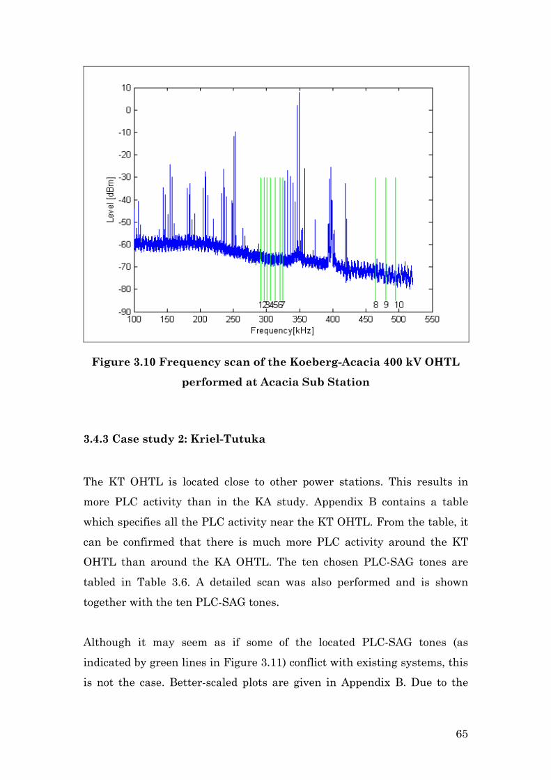
Figure 3.10 Frequency scan of the Koeberg-Acacia 400 kV OHTL
performed at Acacia Sub Station
3.4.3 Case study 2: Kriel-Tutuka
The KT OHTL is located close to other power stations. This results in
more PLC activity than in the KA study. Appendix B contains a table
which specifies all the PLC activity near the KT OHTL. From the table, it
can be confirmed that there is much more PLC activity around the KT
OHTL than around the KA OHTL. The ten chosen PLC-SAG tones are
tabled in Table 3.6. A detailed scan was also performed and is shown
together with the ten PLC-SAG tones.
Although it may seem as if some of the located PLC-SAG tones (as
indicated by green lines in Figure 3.11) conflict with existing systems, this
is not the case. Better-scaled plots are given in Appendix B. Due to the
65
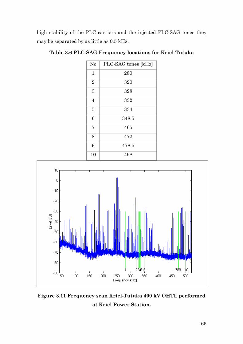
high stability of the PLC carriers and the injected PLC-SAG tones they
may be separated by as little as 0.5 kHz.
Table 3.6 PLC-SAG Frequency locations for Kriel-Tutuka
No PLC-SAG tones [kHz]
1 280
2 320
3 328
4 332
5 334
6 348.5
7 465
8 472
9 478.5
10 498
Figure 3.11 Frequency scan Kriel-Tutuka 400 kV OHTL performed
at Kriel Power Station.
66

3.5 Conclusion
The two case studies are introduced. For the first case study, a short non-
transposed standard transmission line was selected and for the second, a
long transposed transmission line.
PLC signal attenuation simulations were performed on both OHTLs. The
optimum coupling technique (with the adequate sensitivity) for each of the
two PLC-SAG systems was found to be the outer phase to ground coupling
at the local station to outer phase to ground coupling at the remote
station. This coupling is also referred to as outer phase to outer phase
coupling.
Two main frequency regions were identified where PLC-SAG monitoring
tones could be coupled. Frequencies were allocated to the ten tones of each
case study. Close co-operation was needed from the relevant power utility
as the tones, called PLC-SAG monitoring tones, were coupled onto an
operational PLC system.
The following chapter will discuss the hardware installations needed to
realise the specially coupled multi PLC-SAG tone monitoring on the
existing live system.
References:
[1] De Villiers, W., Prediction and measurement of Power Line Carrier
signal attenuation and fluctuation, MScEng Thesis, University of
Stellenbosch, November 2001.
67

[2] L.M. Wedepohl, “Wave propagation in polyphase transmission
systems – Resonance effect due to discretely bonded earth wires”, IEE
proceedings, Volume 112, No. 11, December 1965, pp. 2113-2119.
[3] Turan Gönen, Electric power transmission system engineering –
Analysis and Design, John Wiley and Sons, New York, 1988.
68

Chapter 4
PLC-SAG experimental installations
4.1 Introduction
The hardware of the experimental PLC-SAG installations transmits and
receives specially coupled PLC-SAG tones in order to measure the
attenuation over a long period of time.
The PLC-SAG logging tones are specially coupled onto to the operational
PLC system and decoupled at the remote station. This needs to be done
without jeopardizing normal PLC operations. Ideally, the coupling should
be done in such a fashion that the optimal PLC-SAG coupling
configuration, as identified in the previous section, is used. The
implementation of this will be discussed in Section 4.2.
There are two hardware models, a simplex PLC-SAG system (Figure 4.1)
and a duplex PLC-SAG system (Figure 4.2). The simplex model was
applied to the two case studies. The duplex system is recommended for a
more permanent installation.
The main difference between the simplex PLC-SAG system and the duplex
PLC-SAG system is, as the name indicates, that the latter system is
capable of both transmitting and receiving tones at both ends. This feature
increases the reliability of the system, which only needs to operate in one
direction. If, however, equipment failure occurs at either the transmitter
or receiver, the overall system will still be functional.
69
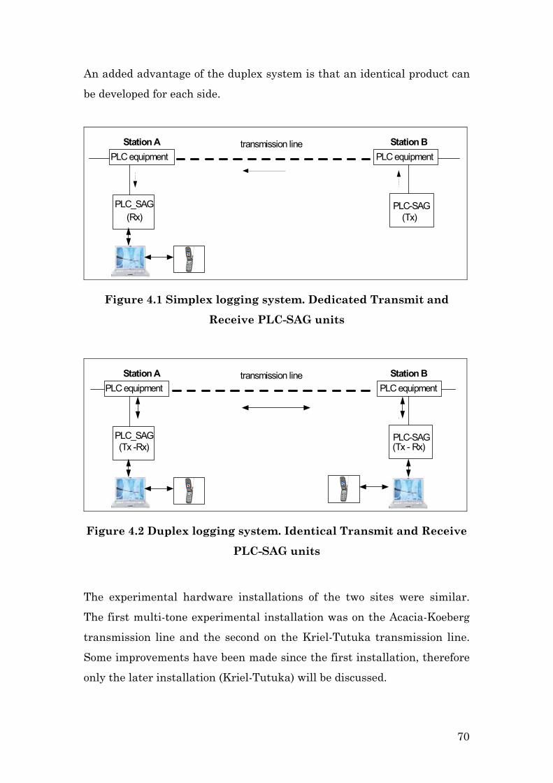
An added advantage of the duplex system is that an identical product can
be developed for each side.
Station A Station B
(Rx)PLC_SAG
(Tx)PLC-SAG
transmission linePLC equipment PLC equipment
Figure 4.1 Simplex logging system. Dedicated Transmit and
Receive PLC-SAG units
Station A Station B
(Tx -Rx)PLC_SAG
(Tx - Rx)PLC-SAG
transmission linePLC equipment PLC equipment
Figure 4.2 Duplex logging system. Identical Transmit and Receive
PLC-SAG units
The experimental hardware installations of the two sites were similar.
The first multi-tone experimental installation was on the Acacia-Koeberg
transmission line and the second on the Kriel-Tutuka transmission line.
Some improvements have been made since the first installation, therefore
only the later installation (Kriel-Tutuka) will be discussed.
70

The outer phase to outer phase coupling configuration is common to both
sides of the installation and to both case studies. An additional
measurement hybrid is used to couple into the existing PLC system and
will be discussed in Section 4.2.
The KT transmitter installation is described in Section 4.3 and the KT
receiver in Section 4.4.
In [1] the author performed a preliminary experiment that coupled a
single tone to the PLC system. The new experimental installation differs
from original the single tone installation because more than one tone or
multi tones are coupled to and decoupled from the PLC system.
4.2 Measuring Hybrid (to incorporate outer phase to
outer phase coupling)
Both simulations indicated that the outer phase to ground coupling at
both stations, performed the best in the context of PLC-SAG system. To
physically incorporate such coupling, an additional signal entry point is
needed in the existing PLC system. By inserting a supplementary
measurement hybrid on the outer phase of the operational system at both
stations, a signal entry point was created. Mr DC Smith, Eskom corporate
Consultant: telecommunication, proposed this technique in the year 2000.
In this section the installation of the supplementary measurement hybrid,
the way it works and the implications for the existing PLC system will be
discussed.
The normal existing hybrid in the PLC system was briefly discussed in
Chapter 2 and will now be discussed in more detail.
71
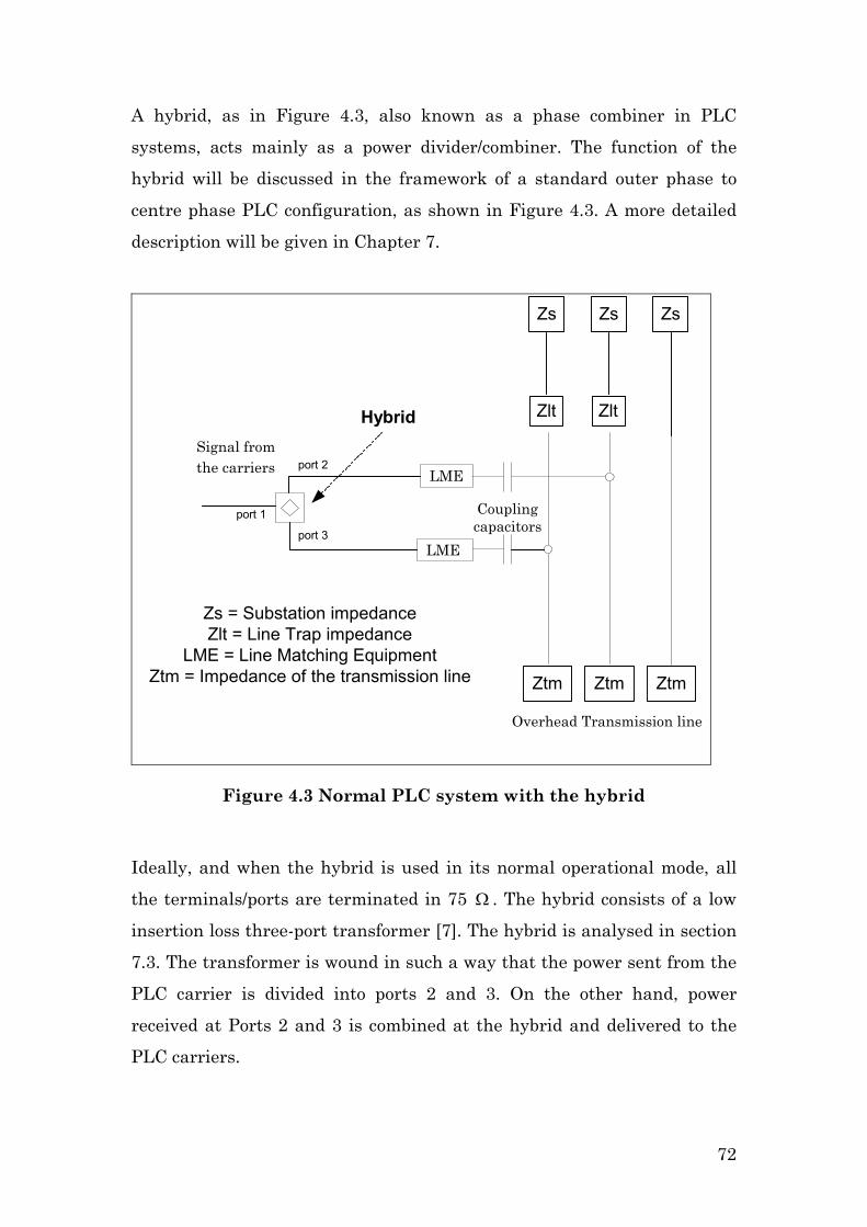
A hybrid, as in Figure 4.3, also known as a phase combiner in PLC
systems, acts mainly as a power divider/combiner. The function of the
hybrid will be discussed in the framework of a standard outer phase to
centre phase PLC configuration, as shown in Figure 4.3. A more detailed
description will be given in Chapter 7.
Overhead Transmission line
LME
Couplingcapacitors
Signal fromthe carriers
Zs Zs Zs
Zlt
LME
Zs = Substation impedanceZlt = Line Trap impedance
LME = Line Matching EquipmentZtm = Impedance of the transmission line
Hybrid
Ztm Ztm Ztm
port 1
port 2
port 3
Zlt
Figure 4.3 Normal PLC system with the hybrid
Ideally, and when the hybrid is used in its normal operational mode, all
the terminals/ports are terminated in 75 Ω . The hybrid consists of a low
insertion loss three-port transformer [7]. The hybrid is analysed in section
7.3. The transformer is wound in such a way that the power sent from the
PLC carrier is divided into ports 2 and 3. On the other hand, power
received at Ports 2 and 3 is combined at the hybrid and delivered to the
PLC carriers.
72

The hybrid is normally configured in such a way that there is a 180
degrees phase shift between the voltage at Port 2 and the voltage at Port
3. Therefore, the standard differential coupling or configuration (Equation
2.4) can be realised via the standard hybrid configuration (Figure 4.3).
The special PLC-SAG outer phase to outer phase coupling can be
practically implemented by inserting an additional hybrid between Port 3
of the standard hybrid and the LME of the outer phase (Figure 4.4).
Overhead Transmission Line
LME
Couplingcapacitors
Signal fromthe carriers
Zs Zs Zs
Zlt
LME
Zs = Substation impedanceZlt = Line Trap impedance
LME = Line Matching EquipmentZ = PLC Input impedance of the outer phase
Ztm = Impedance of the transmission line
PLC-SAG system
port 2
port 3
port 1
Ztm Ztm Ztm
port 1A
port 2A port 3A
Hybrid
Measurement Hybrid
Zlt
Figure 4.4 Measurement Hybrid for the PLC-SAG system
The function of the hybrid is the same as described in the previous section.
The power at Port 1A is divided to Port 2A and Port 3A for a well
terminated hybrid and Port 2A will be isolated from Port 3A (More detail
about this in Chapter 7). The signal at Port 3A would be coupled to Port
1A with a 3 dB loss and would be isolated from Port 2A. Therefore, a
73

signal from the PLC-SAG is coupled and decoupled on the outer phase of
the system, if the same hybrid topology is used at the remote side.
The coupling relationship between the centre phase and outer phase is
also affected. The signal at Port 3, from the carrier, is attenuated by an
extra 3 dB before it is coupled to the outer phase via the measurement
hybrid. The effective coupling configuration for the carrier signals
therefore changes from Equation 2.4 to the coupling configuration shown
in Equation 4.1.
1
2
3
1/ 210
p
a p
p
VV V
V
− = =
4.1
It can be noted that the only difference between Equation 2.4 and
Equation 4.1 is a factor 2 in the amplitude of V . This factor is due to
the power splitting characteristic of the hybrid.
1p
In Chapter 2 the modal power distribution between the modes for the
standard coupling configuration (Figure 4.3) was computed to be 75%
Mode 1 (least attenuated), 25% mode 2 and 0% Mode 3. The modal power
for the coupling configuration in Equation 4.1 was computed to be 81.4%
mode 1, 16.7% mode 2 and 1.9% mode 3. It is clearly evident that more
power is coupled to Mode 1 via the changed coupling configuration
(Equation 4.1) when compared to the standard coupling configuration.
Therefore, it is no surprise that more detailed simulations proved that the
PLC system’s reliability is not compromised by adding the measurement
hybrid on the outer phase. In fact, in some cases the overall system
attenuation is better, where the 3 dB loss in the outer phases due to the
measurement hybrid is more than compensated for by the lesser OHTL
loss, due to the more efficient coupling configuration. Photograph 4.1
shows an installed additional hybrid.
74

In the next section, the transmitter installation at Tutuka Power Station
will be described. The transmitter was connected to Port 3A (Figure 4.4) at
the sending station and the receiver, at the remote station, was also
connected to Port 3A. As mentioned before, the measurement hybrid
installations were similar at both stations.
Photograph 4.1 Installation of a measurement hybrid
4.3 Case 2: Transmitter at Tutuka Power Station
The main function of the Tutuka installation was to couple 10 different
experimental tones sequentially on the outer phase of the OHTL. The
different frequencies are given in Chapter 3.
75
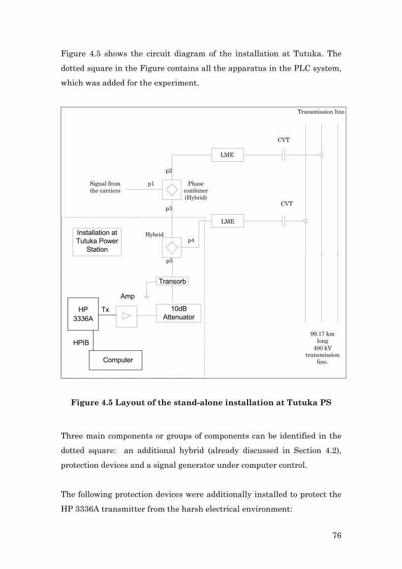
Figure 4.5 shows the circuit diagram of the installation at Tutuka. The
dotted square in the Figure contains all the apparatus in the PLC system,
which was added for the experiment.
Transmission line
LME
CVT
LME
CVT
Signal fromthe carriers
Phasecombiner(Hybrid)
p1
p2
p3
p4
p5
Hybrid
99.17 kmlong
400 kVtransmission
line.
HP3336A
Tx
Computer
HPIB
Transorb
10dBAttenuator
Installation atTutuka Power
Station
Amp
Figure 4.5 Layout of the stand-alone installation at Tutuka PS
Three main components or groups of components can be identified in the
dotted square: an additional hybrid (already discussed in Section 4.2),
protection devices and a signal generator under computer control.
The following protection devices were additionally installed to protect the
HP 3336A transmitter from the harsh electrical environment:
76
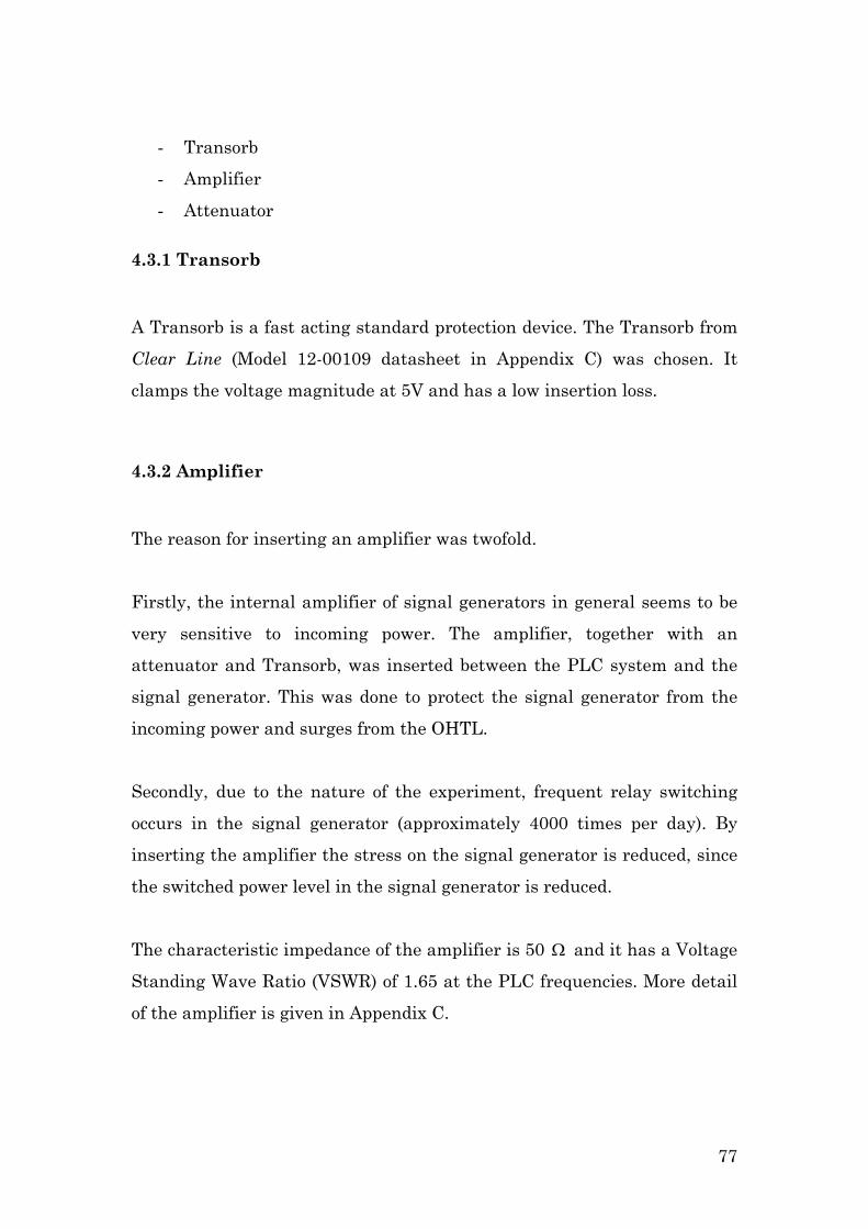
- Transorb
- Amplifier
- Attenuator
4.3.1 Transorb
A Transorb is a fast acting standard protection device. The Transorb from
Clear Line (Model 12-00109 datasheet in Appendix C) was chosen. It
clamps the voltage magnitude at 5V and has a low insertion loss.
4.3.2 Amplifier
The reason for inserting an amplifier was twofold.
Firstly, the internal amplifier of signal generators in general seems to be
very sensitive to incoming power. The amplifier, together with an
attenuator and Transorb, was inserted between the PLC system and the
signal generator. This was done to protect the signal generator from the
incoming power and surges from the OHTL.
Secondly, due to the nature of the experiment, frequent relay switching
occurs in the signal generator (approximately 4000 times per day). By
inserting the amplifier the stress on the signal generator is reduced, since
the switched power level in the signal generator is reduced.
The characteristic impedance of the amplifier is 50 Ω and it has a Voltage
Standing Wave Ratio (VSWR) of 1.65 at the PLC frequencies. More detail
of the amplifier is given in Appendix C.
77

4.3.3 Attenuator in the transmitter circuit
The main function of the attenuator in the experimental setup as shown in
Figure 4.5 was to match the 50 Ω characteristic impedance of the
amplifier to the 75 characteristic impedance of the PLC system. A
secondary function is to attenuate all power levels from the PLC system so
that the amplifier’s output is protected. The mathematics that relates to
the matching of the amplifier will now be discussed.
Ω
Equation 4.2 shows the relationship between VSWR and the magnitude of
the reflection coefficient ( Γ )[2].
11
VSWRVSWR
−Γ =
+ 4.2
where
je θΓ = Γ 4.3
Applying Equation 4.2, to the worst case VSWR = 1.65 of ZHL-32A
amplifier from Mini Circuits (Appendix C), the worst-case magnitude of
the reflection coefficient is 0.245.
The impedance can now be formulated as [2]:
011LZ Z + Γ
=− Γ
4.4
By inserting Equation 4.3 and 0 50Z = Ω into Equation 4.4, for a range of
θ , the worst-case impedance of the amplifier can be simulated. The result
of the simulation is shown in Figure 4.6 (the outer red circle). It can be
noted that the impedance varied from approximately 30.25 Ω to 82.5 Ω
on the real axis.
78
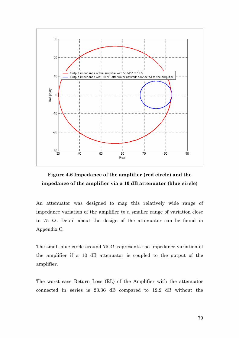
Figure 4.6 Impedance of the amplifier (red circle) and the
impedance of the amplifier via a 10 dB attenuator (blue circle)
An attenuator was designed to map this relatively wide range of
impedance variation of the amplifier to a smaller range of variation close
to 75 . Detail about the design of the attenuator can be found in
Appendix C.
Ω
The small blue circle around 75 Ω represents the impedance variation of
the amplifier if a 10 dB attenuator is coupled to the output of the
amplifier.
The worst case Return Loss (RL) of the Amplifier with the attenuator
connected in series is 23.36 dB compared to 12.2 dB without the
79
attenuator. This improvement is important to ensure that the additional
hybrid is properly terminated.
4.3.4 Signal generator under computer control
The HP 3336A signal generator is used. This particular signal generator
seems to be quite reliable when compared to previous generators used as
no problems were experienced. Photograph 4.2 depicts the HP3336A and a
HP85 control computer. At Tutuka PS the HP3336A is controlled via a
more modern Desktop computer through the Hewlett Packard Interface
Bus (HPIB).
Photograph 4.2 An HP3336A signal generator together with an
HP85 computer in the Lab
The HP 3336A signal generator is controlled in such a way that tones at
specified frequencies are generated sequentially. These tones are each
transmitted for 22 seconds. The tone is “blanked” when the generator
shifts frequency to generate the following tone. A program was written in
HPVEE that controls the instrument, so that it steps through the tones
via the HPIB.
80

4.4 Case 2: Receiver at Kriel Power Station
The installation at Kriel PS is designed to measure the attenuation of the
signals transmitted from Tutuka PS in a synchronised way.
Figure 4.7 shows the components (in the dotted square) of the receiver
installation. The installation consists mainly of an attenuator, 2 receivers,
a computer with instrument control software and a cell phone modem.
Transmission line
LME
CVT
LME
CVT
Signal fromthe carriers
Phasecombiner(Hybrid)
p1
p2
p3
p1A
p3A
Hybrid
99.17 kmlong
400 kVtransmission
line.
W+GPSM
Computer
RS 232
10dBAttenuator
Installation atKriel Power
Station
Cell phoneModem
RS 232
HP3586A
Rx
HBIP
p2A
Figure 4.7 Layout of the stand-alone installation at Kriel Power
Station
81

4.4.1 Attenuator in the receiver circuit
It is important to note that the attenuator at Kriel PS is not used as a
matching device because the receiver has an impedance of 75 . In the
receiver circuit the level of attenuation needs to be considered in more
detail.
Ω
The size of the attenuator was chosen to provide adequate isolation
between the local carriers and the sensitive receiver. The power level at
the instrument can be calculated as:
4.5 _ _ _In Max C H S H M ATTPL P PL PL PL= − − −
where
inPL = Power Level at the instrument due to the local carriers
_Max cP = Maximum power of the carriers
_S HPL = Power Loss due to the Standard Hybrid
_M HPL = Power Loss due to the Measurement Hybrid
ATTPL = Power Loss due to Attenuator
The carriers only operate for a short duration at the maximum power level
when a trip signal is transmitted. At Kriel Power Station 80 Watt ( _Max CP )
carriers are installed. The loss of the Standard Hybrid between P1 and P3
is 3 dB ( _H SPL ) and the loss for the Measurement Hybrid between P2a and
P3a is typically 25 dB ( _H MPL ) if well terminated (Figure 4.7). Therefore,
by using Equation 4.5 the Power Level at the instrument ( ) due to the
local carriers is 12.67 mW for a 10 dB attenuator ( ). The instrument
can measure up to 1W and therefore the calculated with the 10 dB
attenuator is within specification.
InPL
ATTPL
PLIn
82

4.4.2 Receivers
The direct height experimental measurement, which is the main
experiment in this thesis (discussed in the following Chapter), was quite
an expensive exercise due to the number of people required in the field for
the measurement. It was therefore crucial that the PLC-SAG hardware
was fully functional at the time of the physical direct height measurement.
Due to the experimental nature of the hardware, frequency errors and
failures occurred. To minimize the risk of experimental failure during the
direct height measurement, two receivers were installed at Kriel Power
Station. In Figure 4.7 the two receivers (selective voltmeters), Hewlett
Packard (HP) HP3586A and Wandel & Goltermann (WG) PSM-137 are
shown. The HP was configured to provide 75 Ω terminations and the WG
measured via the high-impedance port. This was done to prevent double
termination. More detail on general settings of the PSM-137 and HP
3586A are given in Appendix C.
Photograph 4.3 The HP 3586A (left/bottom) and Wandel &
Goltermann PSM-137 (left/top) under computer control - testing
the system.
83
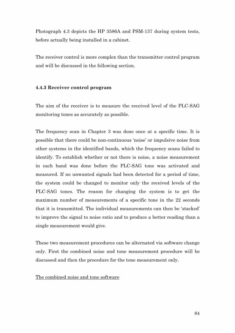
Photograph 4.3 depicts the HP 3586A and PSM-137 during system tests,
before actually being installed in a cabinet.
The receiver control is more complex than the transmitter control program
and will be discussed in the following section.
4.4.3 Receiver control program
The aim of the receiver is to measure the received level of the PLC-SAG
monitoring tones as accurately as possible.
The frequency scan in Chapter 3 was done once at a specific time. It is
possible that there could be non-continuous ‘noise’ or impulsive noise from
other systems in the identified bands, which the frequency scans failed to
identify. To establish whether or not there is noise, a noise measurement
in each band was done before the PLC-SAG tone was activated and
measured. If no unwanted signals had been detected for a period of time,
the system could be changed to monitor only the received levels of the
PLC-SAG tones. The reason for changing the system is to get the
maximum number of measurements of a specific tone in the 22 seconds
that it is transmitted. The individual measurements can then be ‘stacked’
to improve the signal to noise ratio and to produce a better reading than a
single measurement would give.
These two measurement procedures can be alternated via software change
only. First the combined noise and tone measurement procedure will be
discussed and then the procedure for the tone measurement only.
The combined noise and tone software
84
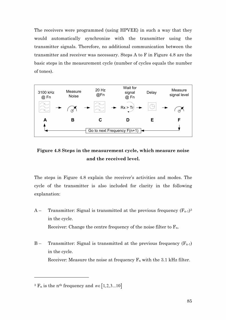
The receivers were programmed (using HPVEE) in such a way that they
would automatically synchronize with the transmitter using the
transmitter signals. Therefore, no additional communication between the
transmitter and receiver was necessary. Steps A to F in Figure 4.8 are the
basic steps in the measurement cycle (number of cycles equals the number
of tones).
3100 kHz@ Fn
20 Hz@Fn Delay
Rx > Tr
Wait forsignal@ Fn
MeasureNoise
Measuresignal level
A B C D E F
Go to next Frequency F(n+1)
Figure 4.8 Steps in the measurement cycle, which measure noise
and the received level.
The steps in Figure 4.8 explain the receiver’s activities and modes. The
cycle of the transmitter is also included for clarity in the following
explanation:
A – Transmitter: Signal is transmitted at the previous frequency (Fn-1)3
in the cycle.
Receiver: Change the centre frequency of the noise filter to Fn.
B – Transmitter: Signal is transmitted at the previous frequency (Fn-1)
in the cycle.
Receiver: Measure the noise at frequency Fn with the 3.1 kHz filter.
3 Fn is the nth frequency and [ ]1, 2,3...10n∈
85

C – Transmitter: Signal is transmitted at the previous frequency in the
cycle.
Receiver: Change the type of filter to the 20 Hz/25 Hz selective
filter.
D- Transmitter: Change frequency to Fn with a soft blanked action.
Receiver: Test the received signal level each second. If the level of
the received signal is more than the threshold of -45 dBm then it
will step to E.
E- Transmitter: Signal is transmitted at Fn.
Receiver: Cycle is delayed by 1 second. The reason for this delay is
the fact that the transmitter is soft blanked. The level of the
transmitter could be greater than the threshold, and therefore
detected in step D, but not yet at full power.
F- Transmitter: Signal is transmitted at Fn.
Receiver: Measures the received signal level at Fn.
While the transmitter is still activated at Fn the receiver goes back to step
A to measure the noise at F(n+1). The transmitter tone will be delayed for
long enough (22 seconds between tones) for the receiver to perform steps A
to D and wait (at step D) for the next tone. This loop will continue to
measure the noise and signal levels for the duration of the experiment.
Tone measurement only
Measurement results for both case studies proved that the frequency
regions had been well identified. No unexpected noise occurred in those
frequency regions.
86

Eliminating steps A and B changed the measurement cycle as shown in
Figure 4.8. The time gained by skipping steps A and B was utilised by
repeating step F five times. Thus the PLC-SAG tone results obtained in
the main experiment, discussed in the following Chapters, were the raw
data average from 5 repeated measurements (Step F) of the relevant tone.
The last hardware component in the receiver is the industrial cell phone,
which will now be discussed.
4.4.4 Industrial cell phone
The control program (In HPVEE) stored the measured levels in a data file.
This file size becomes larger as more and more measurements accumulate.
The main power supply of the computer is connected to a timer. The timer
switches the computer off once a week, for approximately 10 minutes at
midnight. As the computer program restarts, a new set of data files is
generated.
These files were then downloaded via the cell phone, which was
convenient, as downloading could be performed at any time and place.
The remote computer (with the external cell phone connected) and the
local computer interface were controlled by a software package called
PCAnyWhere. The software needs to be installed on both computers. In
this KT case study the remote computer was at the Kriel Power Station
together with the rest of the PLC-SAG receive system. The local computer
was in Stellenbosch most of the time. The local computer communicates
with the remote computer to enable data download or PLC-SAG software
updates.
87

4.5 Conclusions
For both case studies, a simplex logging methodology was used as
explained by Figure 4.1.
Due to the nature of the hardware (equipment designed to work in
laboratories) frequent hardware failures occurred. Adding extra protective
devices to the system, additional to the standard PLC protection devices,
improved the robustness of the experimental installations. Two receivers
were installed at Kriel Power Station to increase the reliability of the
installations.
Both experimental installations of the two case studies were fully
operational during the direct height measurement, which was essential.
The direct height measurement will be discussed in the following chapter.
The results from the logging stations will be presented in Chapter 6, as
they will be compared to the simulations and the direct height
measurements.
References:
[1] De Villiers, W., Prediction and measurement of Power Line Carrier
signal attenuation and fluctuation, MScEng Thesis, University of
Stellenbosch, November 2001.
[2] R.E. Ziemer and W.H. Tranter, Principles of Communications,
Fourth Edition, John Wiley & Sons, 1988.
88

Chapter 5
Direct height measurements
5.1 Introduction
This chapter focuses on measuring the average conductor height of the
whole OHTL. The average height variation of the conductor above the
ground is estimated by taking the average of three direct height
measurements of well-spaced spans.
The measurement commenced by selecting an appropriate instrument.
Four instruments were tested on a live OHTL trial. These tests and the
associated finding will be discussed in Section 5.2.
The average height measurement methodology will be introduced in
Section 5.3. The methodology comprises i) selecting appropriate sites, ii)
marking the specific measuring points with pegs, iii) surveying the span
and iv) performing continuous direct conductor height measurements.
The four steps will be further discussed, as applied to each case study, in
Section 5.4 to Section 5.7.
The transformation of the individual height measurements to the average
height of the OHTL is discussed in Section 5.8.
89
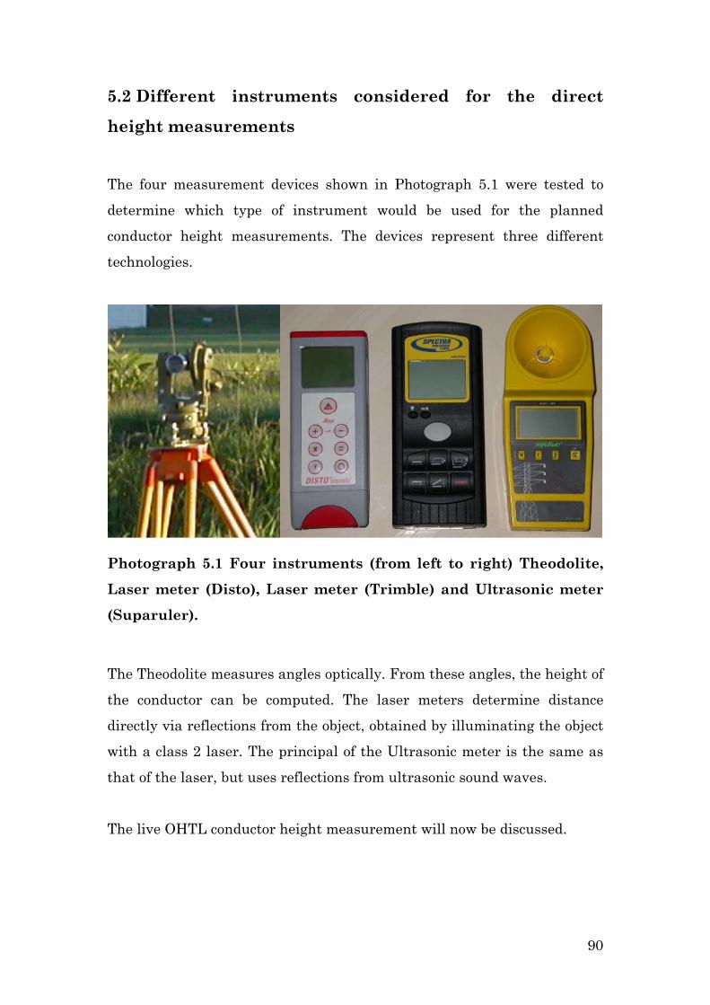
5.2 Different instruments considered for the direct
height measurements
The four measurement devices shown in Photograph 5.1 were tested to
determine which type of instrument would be used for the planned
conductor height measurements. The devices represent three different
technologies.
Photograph 5.1 Four instruments (from left to right) Theodolite,
Laser meter (Disto), Laser meter (Trimble) and Ultrasonic meter
(Suparuler).
The Theodolite measures angles optically. From these angles, the height of
the conductor can be computed. The laser meters determine distance
directly via reflections from the object, obtained by illuminating the object
with a class 2 laser. The principal of the Ultrasonic meter is the same as
that of the laser, but uses reflections from ultrasonic sound waves.
The live OHTL conductor height measurement will now be discussed.
90
5.2.1 Setup for the direct height measurement
The height variation of the conductor between towers 2 and 3 of the 400
kV transmission line between Acacia Substation and Koeberg Power
Station was measured. Measurement stations were placed underneath the
outer conductor of the phase bundle. In total, three measurement stations
were defined. Two of the stations were directly beneath the outer
conductor of the transmission line’s phase bundle, and the third station
was approximately 30 m to the side of the outer bundle of the OHTL.
Photograph 5.2 shows the three measuring stations on the yellow tripods.
The stations were named, from left to right, Station A, B and C.
A B C
Photograph 5.2 Three measurement stations
5.2.2 Measurements
During the execution of the measurements the following was noted. The
theodolite was difficult to set up, especially in the sandy environment of
the KA OHTL. Both the theodolite and the laser meters were difficult to
operate in windy conditions.
91

Figure 5.1 shows the results from the four different measurement devices,
all referred to measurement Station A. Five measurement results can be
noted in Figure 5.1 obtained from the two fixed lasers at stations A and B
(which were on tripods), the theodolite (also on a tripod) at measurement
station C and the handheld ultrasonic meter at stations A and B.
It can be noted that all the data have not continuous. Measurements from
the ultrasonic instrument indicated the most interruption; the reason is
uncertain, but the instrument gave frequent errors. The laser meter at
station A (Trimble) did not produce any readings between 7:15 and 8:00.
At that stage, some level of moisture affected all the instruments. After
the moisture evaporated the instruments seemed to work correctly. A
strong wind appeared at 15:30. The Disto laser at Station A was unable to
measure the conductor height in the strong windy conditions (around
17:00). Due to a difficult setup procedure, the theodolite was only
operational from midday onwards.
Figure 5.1 Conductor heights, measured on Saturday 26 April
2003, via the four different instruments
92

From Figure 5.1, it can be seen that the two laser instruments correlate
the best with each other. The correlation between the ultrasonic
measurement and the lasers was close during the early morning. The
variation between subsequent measurements was greatest for the
ultrasonic measurements. Although the device was not mounted on a
tripod (as were the other instruments), great care was taken to position it
accurately for the measurements. Results from the theodolite and the
lasers showed a relatively small average difference of approximately 5 cm
between 12:00 and 15:00. After the wind strengthened the difference
increased.
5.2.3 Conclusion of the OHTL conductor height measurement trial
It was concluded that the laser devices were the best, considering
accuracy, cost, robustness, reliability and operational simplicity. More
specifically a ‘Disto™ pro’ laser was chosen which is manufactured by
Leica Geosystems.
The only concern when using the laser meter was the fact that unreliable
measurement occurred during windy conditions. It was later found that
the laser instrument could be purchased with an additional telescopic
viewer, which enabled the laser operator to ‘track’ the conductor in windy
conditions. This worked well, as the direct height measured data
presented later in this thesis are uninterrupted, unlike the data presented
in Figure 5.1.
Photograph 5.3 shows the laser meter with the telescopic viewer. Three
lasers (all the same make and model - ‘Disto™ pro’), with telescopic
viewers, were used from then onwards in the research to measure the
height of the OHTL conductor.
93

Photograph 5.3 ‘Disto™ pro’ laser with telescopic viewer
5.3 The measurement methodology
The following are steps in the methodology used to measure the average
height of the OHTL for the two case studies.
Step 1) Select three OHTL spans that are relatively long, easily
accessible and well spaced from one other.
Step 2) Determine more or less the centre point of the span and then
find an easily identifiable point on the conductor itself to be measured.
This easily identifiable point is called the upper ‘fixed’ point, which
cannot move in the direction of the transmission line. The conductor
spacer keeps the individual conductors of a bundle conductor in place.
It is ideal to choose the phase combiner as the upper ‘fixed’ point on the
conductor. Mark the location directly underneath the upper fixed point
with a peg. Now there are two ‘fixed’ points, the upper located on the
conductor itself and the lower being the peg on the ground. The height
movement of the upper point relative to the peg can now be measured.
If the experiment is repeated on a different day, using the same ‘fixed’
94
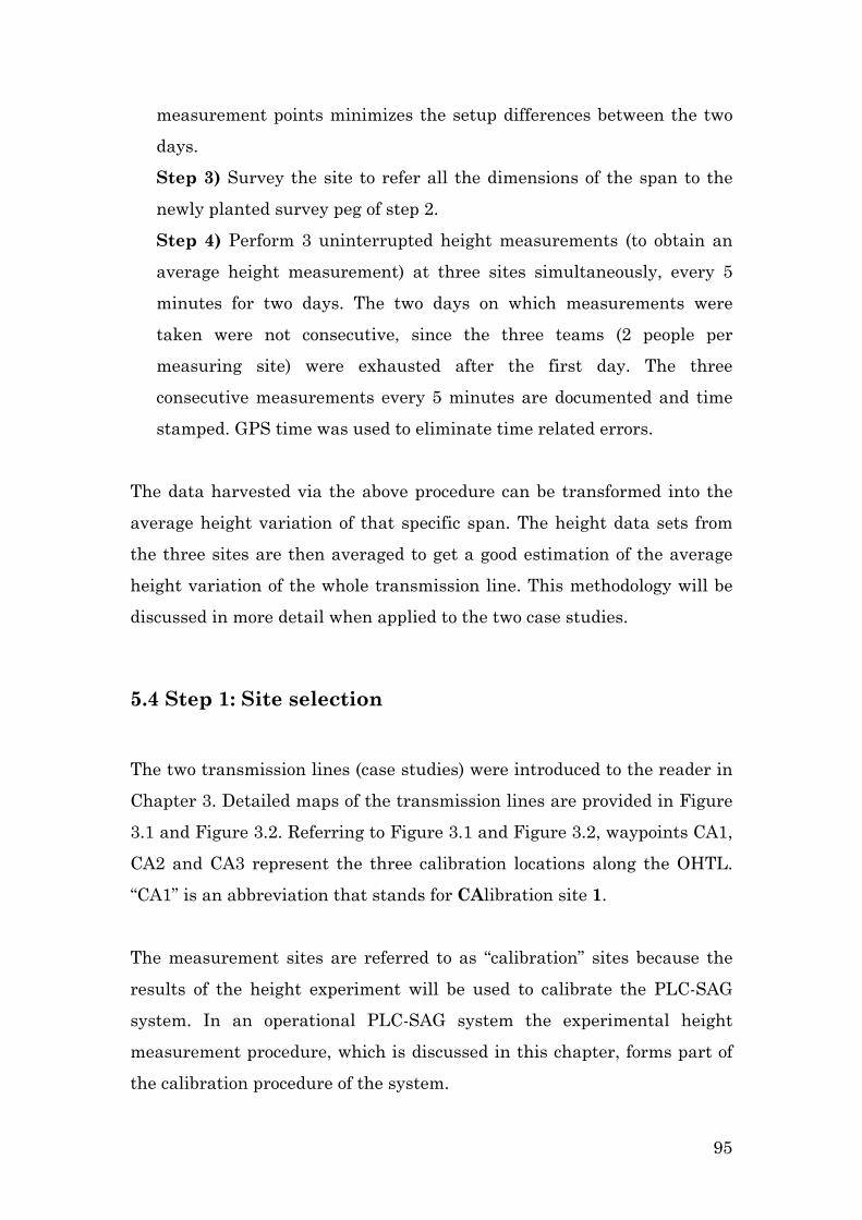
measurement points minimizes the setup differences between the two
days.
Step 3) Survey the site to refer all the dimensions of the span to the
newly planted survey peg of step 2.
Step 4) Perform 3 uninterrupted height measurements (to obtain an
average height measurement) at three sites simultaneously, every 5
minutes for two days. The two days on which measurements were
taken were not consecutive, since the three teams (2 people per
measuring site) were exhausted after the first day. The three
consecutive measurements every 5 minutes are documented and time
stamped. GPS time was used to eliminate time related errors.
The data harvested via the above procedure can be transformed into the
average height variation of that specific span. The height data sets from
the three sites are then averaged to get a good estimation of the average
height variation of the whole transmission line. This methodology will be
discussed in more detail when applied to the two case studies.
5.4 Step 1: Site selection
The two transmission lines (case studies) were introduced to the reader in
Chapter 3. Detailed maps of the transmission lines are provided in Figure
3.1 and Figure 3.2. Referring to Figure 3.1 and Figure 3.2, waypoints CA1,
CA2 and CA3 represent the three calibration locations along the OHTL.
“CA1” is an abbreviation that stands for CAlibration site 1.
The measurement sites are referred to as “calibration” sites because the
results of the height experiment will be used to calibrate the PLC-SAG
system. In an operational PLC-SAG system the experimental height
measurement procedure, which is discussed in this chapter, forms part of
the calibration procedure of the system.
95

The following factors need to be considered when locating the sites:
- Preferably close to a road and easily accessible. It can be noted, in
studying Figure 3.1 and Figure 3.2, that all six CA sites were
located close to a nearby road.
- Sites should be well spaced from each other, but must represent the
whole transmission line.
- The span on which height measurements are to be made has to be
relatively long, since this increases the measurement sensitivity.
5.4.1 Case 1: Koeberg-Acacia (KA)
In Figure 5.2 the calibration sites are plotted next to each other as a
function of distance along the length of the OHTL. From Figure 5.2, it can
be seen that the sites are well spaced. The span lengths of the relevant
spans are given, also indicated in Figure 5.2. The span lengths of CA1 and
CA3 are longer than the ruling span (347.36m, as computed in Chapter 3
for the simulation) and the CA2 span is 2.2m shorter. The tower number
in the figure is shown as KA X, which represents Koeberg-Acacia tower
number X. The towers are numbered from Acacia to Koeberg and not from
Koeberg to Acacia as one might have deduced from the sequence of the ‘K’
and the ‘A’.
96

0 1/4*L 1/2*L 3/4*L L
CA1 CA2 CA3
0.5km
29.4km16.3km
31.318km
349.67m
KA2
KA3
Acacia Koeberg
345.16m
KA51
KA52
375.04m
KA88
KA89
Figure 5.2 Locations of the calibration points on the 400 kV
Koeberg-Acacia transmission line as a function of length.
5.4.2 Case 2: Kriel-Tutuka (KT)
The KT OHTL is 99.5 km long and is therefore approximately three times
longer than the KA OHTL. Figure 5.3 shows the locations of the different
CA sites. All the spans are longer than the ruling span (404.157m) of the
OHTL.
97

0 1/4*L 1/2*L 3/4*L L
KT1 KT2 KT3
4.6km
86.8km53.1km
99.5km
Kriel PS Tutuka PS
412.617m
KT14
KT15
469m
KT132
KT133
483.777m
KT230
KT231
Figure 5.3 Locations of the calibration points on the 400 kV Kriel-
Tutuka transmission line.
The following step in the average height measurement methodology will
now be discussed.
5.5 Step 2: Marking measurement points at selected sites
Once the CA site is selected, the upper and lower ‘fixed’ points need to be
established by locating the approximate centre of the span. The spans are
in the order of 450 m long and one cannot rely on a naked eye judgement.
Photograph 5.4 depicts an instrument (Bushnell Range Finder), which can
assist in obtaining an indication of the centre point of the span.
98

Photograph 5.4 Bushnell range finder
After the centre of the span is identified, the closest bundle combiner
needs to be located. Directly under the conductor spacer, a peg can be
planted. The selection of the peg depends on the type of soil. Photograph
5.5 depicts the peg that was used in the KT OHTL’s hard muddy type of
soil. At KA, the soil is sandier; therefore longer thinner pegs were used.
The top of the peg was marked with red paint for easy identification.
Photograph 5.5 Showing a peg made of railway sleeper (used as
the lower ‘fixed’ point) together with the laser meter
99

The laser meter can then be set up above the peg for measurements. The
laser meter is aimed at the conductor spacer (the upper fixed point)
Photograph 5.6 depicts the red laser dot of the instrument aimed at the
conductor where the phase combiner is located.
Photograph 5.6 Location where the conductor height was
measured – the red dot on the outer phase of the conductor. (Used
as the upper ‘fixed’ point)
5.6 Step 3: Measurement site survey
In the Tables in Appendix A, details of the spans are given. It is difficult to
apply all the span detail available to the newly planted peg. Therefore a
site survey was conducted to obtain accurate data, which is correctly
referred to the newly planted survey pegs.
At the first sites measured (CA1-CA3 at KT) a level meter (dumpy-meter),
laser meter and a “range finder” were used. It took one day to measure two
100

sites because the range of the dumpy level meter is only approximately 70
m. During the second set of survey measurements for KA, a “total station”
was used which can measure longer distances. Using the ‘total station’ all
three sites can easily be surveyed in one day. Figure 5.4 shows all the
relevant lengths (A-D) to be measured during the survey. E is the height
difference between the upper and lower ‘fixed’ points, which is measured
to compute the average height variation.
Figure 5.4 Dimensions of a typical span
The results of the surveys are tabled in Table 5.1
101
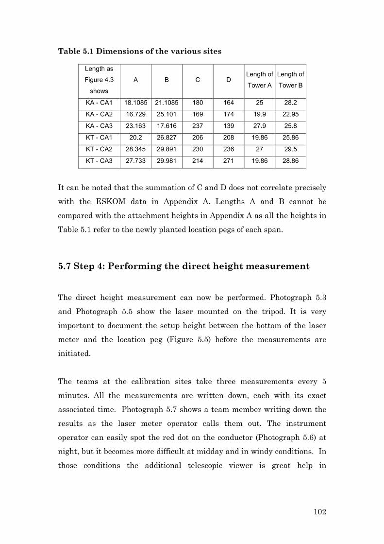
Table 5.1 Dimensions of the various sites
Length as
Figure 4.3
shows
A B C D Length of
Tower A
Length of
Tower B
KA - CA1 18.1085 21.1085 180 164 25 28.2
KA - CA2 16.729 25.101 169 174 19.9 22.95
KA - CA3 23.163 17.616 237 139 27.9 25.8
KT - CA1 20.2 26.827 206 208 19.86 25.86
KT - CA2 28.345 29.891 230 236 27 29.5
KT - CA3 27.733 29.981 214 271 19.86 28.86
It can be noted that the summation of C and D does not correlate precisely
with the ESKOM data in Appendix A. Lengths A and B cannot be
compared with the attachment heights in Appendix A as all the heights in
Table 5.1 refer to the newly planted location pegs of each span.
5.7 Step 4: Performing the direct height measurement
The direct height measurement can now be performed. Photograph 5.3
and Photograph 5.5 show the laser mounted on the tripod. It is very
important to document the setup height between the bottom of the laser
meter and the location peg (Figure 5.5) before the measurements are
initiated.
The teams at the calibration sites take three measurements every 5
minutes. All the measurements are written down, each with its exact
associated time. Photograph 5.7 shows a team member writing down the
results as the laser meter operator calls them out. The instrument
operator can easily spot the red dot on the conductor (Photograph 5.6) at
night, but it becomes more difficult at midday and in windy conditions. In
those conditions the additional telescopic viewer is great help in
102

measuring accurately. The measured results from the two case studies will
now be discussed.
Laser
Tripod
Location peg
Ground level
Setup height
Figure 5.5 Measurement set-up at a site
Photograph 5.7 Mr P Pretorius recording the measurements at KT
CA2 with the GPS located on the table for GPS time.
103

5.7.1Case study: KA (Direct height measurement above peg)
The three CA points on the KA OHTL were measured during two days, 5th
and 12th October 2004, from early morning till mid afternoon. The results
are plotted in Figure 5.6. The height variations above the pegs cannot be
compared directly, due to the different span lengths and measurement
points. Generally, it can be noted that the conductor sagged to its
maximum on 5th October around 11:30 in the morning. During the next
day of measurements the maximum sag occurred noticeably at 11:30, only
this time at CA3. The other sites had not sagged to their maximum before
the experiment was stopped. This highlights the fact that measuring only
one site’s height variation could have been misleading in the framework of
this study.
00:00 06:00 12:00 18:00 00:00 06:00 12:00 18:00 00:008.5
9
9.5
10
10.5
11
Hei
ght a
bove
peg
Time
CA1CA2CA3
2004/10/05 2004/10/12
Figure 5.6 Direct height measurement above the pegs of KA
104
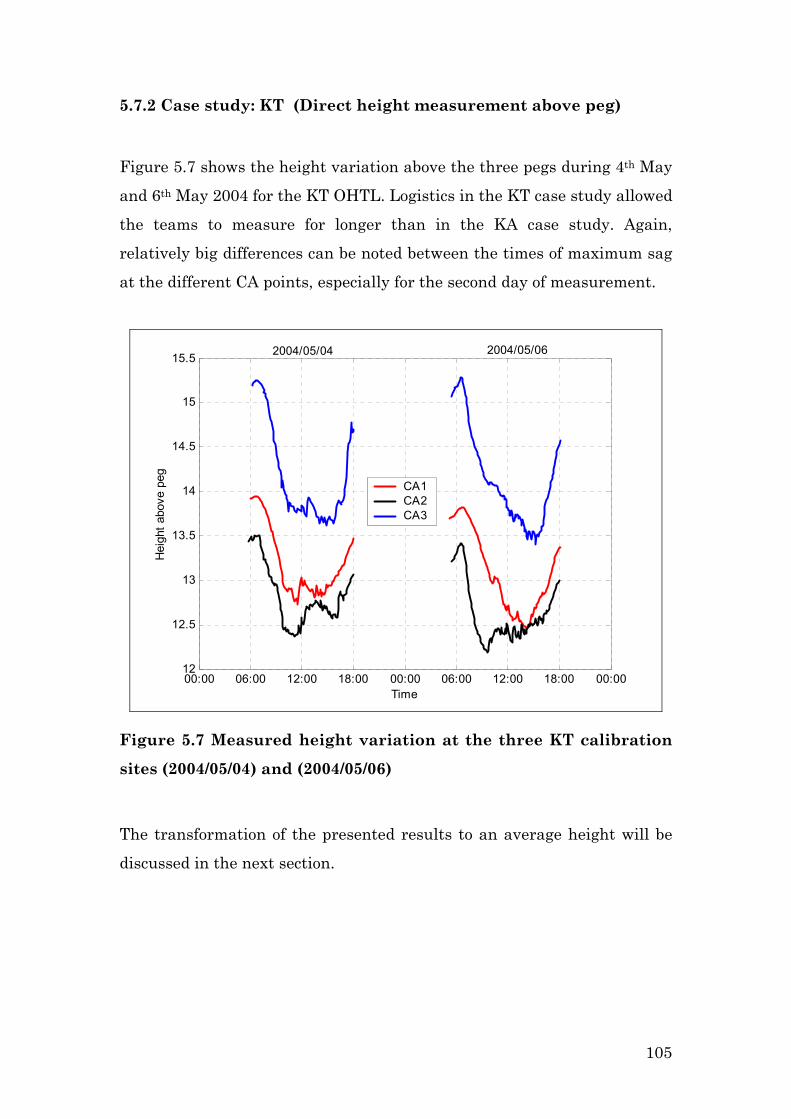
5.7.2 Case study: KT (Direct height measurement above peg)
Figure 5.7 shows the height variation above the three pegs during 4th May
and 6th May 2004 for the KT OHTL. Logistics in the KT case study allowed
the teams to measure for longer than in the KA case study. Again,
relatively big differences can be noted between the times of maximum sag
at the different CA points, especially for the second day of measurement.
00:00 06:00 12:00 18:00 00:00 06:00 12:00 18:00 00:0012
12.5
13
13.5
14
14.5
15
15.5
Time
Hei
ght a
bove
peg
CA1CA2CA3
2004/05/04 2004/05/06
Figure 5.7 Measured height variation at the three KT calibration
sites (2004/05/04) and (2004/05/06)
The transformation of the presented results to an average height will be
discussed in the next section.
105

5.8 Transforming to the average height
In order to explain this section, the focus will be on KA CA1 (Figure 5.8).
The dotted vertical line in the middle of the graph represents the location
where the OHTL conductor height movement was observed. The OHTL
conductor is plotted for a range of different heights in Figure 5.8. If the
observation point moves, the results of the direct height measurement will
be correspondingly different, for the same range of conductor heights.
Therefore, the direct height measurements at the sites need to be
transformed to the average height measurement of the span.
Figure 5.8 Layout of KA - CA1 and measurement point
A program (in MatLab) was written to produce a transformation graph. In
the graph the measured data at a specific location along the span (x-axis)
is transformed to the average height variation of the span (y-axis). The
program is based on typical sag formulas, as described in [1] and needs all
106

the relevant dimensions as described in Figure 5.4. Figure 5.9 shows the
transformation graph for KA CA1. The graph can be used as a lookup
table. For example: if the direct height measurement is 9 m (measured 180
m from tower 2) the average height of the span is 12.75 m above an ideal
ground plane (an ideal ground plane is a straight line between the two
bases of the relevant towers as drawn in Figure 5.8).
Figure 5.9 Average height movement of the conductor above a
perfect ground plane for the calibration point KA - CA1
The three average height data sets for a case study are added and then
divided by three to get an estimation of the average height of the whole
transmission line. Figure 5.10 and Figure 5.11 shows the estimated
average height for the two case studies via three direct height
measurement sites per case study. Comparing the two sets of results, it
can be noted that there was a greater variation present in the second case
study, KT OHTL. From the results it was also evident that the average
height of the conductor at KT OHTL was greater than that of the KA
107

OHTL. It has been confirmed that ESKOM re-tensioned the KT OHTL to a
higher rating, due to the importance of the line. This also implies that the
average conductor height is higher after the line had been re-tensioned.
00:00 06:00 12:00 18:00 00:00 06:00 12:00 18:00 00:0013.6
13.7
13.8
13.9
14
14.1
14.2
14.3
Ave
rage
hei
ght o
f the
con
duct
or
Time
2004/10/05 2004/10/12
Figure 5.10 Estimated average height variation of the KA OHTL
(Case study 1)
108
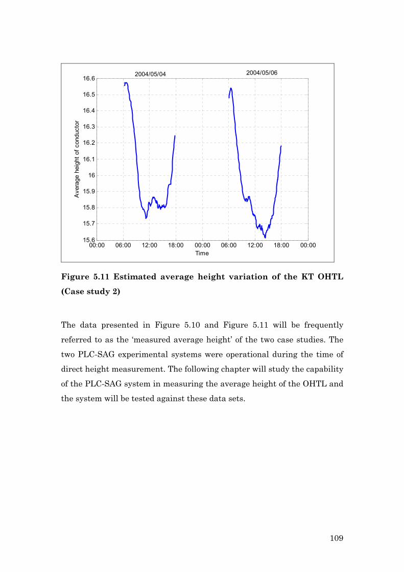
00:00 06:00 12:00 18:00 00:00 06:00 12:00 18:00 00:0015.6
15.7
15.8
15.9
16
16.1
16.2
16.3
16.4
16.5
16.6
Time
Ave
rage
hei
ght o
f con
duct
or2004/05/04 2004/05/06
Figure 5.11 Estimated average height variation of the KT OHTL
(Case study 2)
The data presented in Figure 5.10 and Figure 5.11 will be frequently
referred to as the ‘measured average height’ of the two case studies. The
two PLC-SAG experimental systems were operational during the time of
direct height measurement. The following chapter will study the capability
of the PLC-SAG system in measuring the average height of the OHTL and
the system will be tested against these data sets.
109
5.9 Conclusions
A laser meter with a telescopic viewer was identified as the most suitable
instrument to measure the direct height of the OHTL conductor.
The measurement methodology is discussed step by step, as applied to the
two case studies. The methodology can be summarised as determining the
site, establishing the specific calibration location at the site, surveying the
site and, lastly, measuring the conductor height continuously for a period
of approximately 7 to 8 hours on two separate occasions.
The direct height measurements above the peg were transformed to the
average height. The data presented in Figure 5.10 and Figure 5.11 will be
used in the following chapter and will be compared with the data produced
by the PLC-SAG system.
References:
[1] Turan Gönen, Electric power transmission system engineering –
Analysis and Design, John Wiley and Sons, New York, 1988.
110

Chapter 6
PLC-SAG system evaluation and
calibration
6.1 Introduction
This chapter addresses the main focus of the study undertaken by
disclosing whether the PLC-SAG system tracks the average height of an
OHTL conductor above ground and, if it does, with what accuracy.
In Chapter 3 two case studies were chosen on which the PLC-SAG system
could be evaluated. The first case study can be classified as a typical
configuration and the second case study as a non-standard scenario, as it
is transposed and comprises 7 different sections (Chapter 3). The latter
case is considered the ultimate test. Simulations created the expectation
that the level of the specially coupled PLC-SAG tones would vary as the
conductor sagged, in both case studies. Chapter 4 focused on the tasks and
challenges associated with the implementation of two PLC-SAG systems
on KA and KT to produce the logged values of the level of the PLC-SAG
tones. Chapter 5, on the other hand, discussed the coordinated effort of
measuring the average conductor height of the OHTLs via three
simultaneous direct measurements.
Chapter 6 will now show the comparison of those results as discussed in
Chapter 3 (Simulations), Chapter 4 (Logged results from the PLC-SAG
111

hardware) and Chapter 5 (Direct height measurements) to study the PLC-
SAG technique.
In this thesis no advanced Digital Signal Processing (DSP) techniques
were used to improve the quality of the data.
This chapter starts by discussing the first case study. The logged data will
be shown and discussed with emphasis on signal level variations. The
attenuation simulations from Chapter 3, for the specially coupled PLC-
SAG tones, are redrawn as a function of height. The simulation and logged
PLC-SAG tones are compared. These tones are correlated with the direct
height measurement as discussed in Chapter 5. From the correlation, the
best tones were identified and combined to get the Principal PLC-SAG
tone. At this point the abovementioned process was repeated for the
second case study.
The Principal PLC-SAG tone level for each of the two case studies was
then calibrated. The calibration technique will be discussed. After the
calibration the Principal PLC tone will be called the PLC-SAG Average
Height Signal (AHS) and is given in meters. PLC-SAG AHS is then
plotted with the direct height measurements and the level of accuracy will
be determined.
6.2 Case study 1 (Koeberg-Acacia) logged tones
6.2.1 Logged PLC-SAG monitoring tones
Figure 6.1 shows the logged data set from the PLC-SAG experimental
system. The red squares in the data sets represent the segment of the data
that will be used in the correlation, as it is at the same time intervals as
those used in the first and second day of direct height measurements. The
112
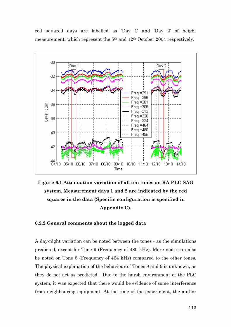
red squared days are labelled as ‘Day 1’ and ‘Day 2’ of height
measurement, which represent the 5th and 12th October 2004 respectively.
Figure 6.1 Attenuation variation of all ten tones on KA PLC-SAG
system. Measurement days 1 and 2 are indicated by the red
squares in the data (Specific configuration is specified in
Appendix C).
6.2.2 General comments about the logged data
A day-night variation can be noted between the tones - as the simulations
predicted, except for Tone 9 (Frequency of 480 kHz). More noise can also
be noted on Tone 8 (Frequency of 464 kHz) compared to the other tones.
The physical explanation of the behaviour of Tones 8 and 9 is unknown, as
they do not act as predicted. Due to the harsh environment of the PLC
system, it was expected that there would be evidence of some interference
from neighbouring equipment. At the time of the experiment, the author
113

was informed by the Station Operator of Acacia (where the receiver
(selective Voltmeter) is located) that a protection relay (called P40) was
giving problems. The operating frequency of the P40 protection relay is
468 kHz to 476 kHz, which is located between tone 8 and tone 9.
Frequent problems occurred due to the experimental nature of the
hardware. The absence of data during the 9-10 October 2004 is due to
logger related problems.
6.2.3 Levels of the received PLC-SAG tones
Various insertion loss experiments and measurements were performed on
this specific OHTL [1]. They will not be repeated, although an analysis
will be done to see whether the received level from the experiment is close
to the expected level. The frequency of PLC-SAG monitoring Tone 3 is 301
kHz and this will be used in this discussion, as it is close to the centre of
the PLC frequency band (100-500 kHz).
The level of the logged Tone 3 (Frequency 301 kHz) varies around –32
dBm (refer to Figure 6.1).
The total attenuation of a PLC-SAG monitoring tone can be expressed as:
6.1 TxPower (2 2 )PLC SAGAtt CL MHL AA SLL− = − ⋅ + ⋅ + +
where
TxPower = Transmit power
CL = Coupling Loss
MHL = Measurement Hybrid Loss
AA = Attenuation of Attenuator
SLL = Simulated Line Loss
114
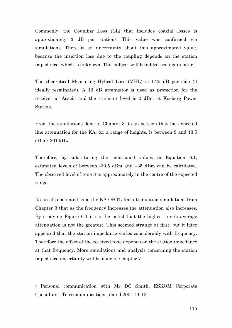
Commonly, the Coupling Loss (CL) that includes coaxial losses is
approximately 3 dB per station4. This value was confirmed via
simulations. There is an uncertainty about this approximated value,
because the insertion loss due to the coupling depends on the station
impedance, which is unknown. This subject will be addressed again later.
The theoretical Measuring Hybrid Loss (MHL) is 1.25 dB per side (if
ideally terminated). A 13 dB attenuator is used as protection for the
receiver at Acacia and the transmit level is 0 dBm at Koeberg Power
Station.
From the simulations done in Chapter 3 it can be seen that the expected
line attenuation for the KA, for a range of heights, is between 9 and 13.5
dB for 301 kHz.
Therefore, by substituting the mentioned values in Equation 6.1,
estimated levels of between -30.5 dBm and –35 dBm can be calculated.
The observed level of tone 3 is approximately in the centre of the expected
range.
It can also be noted from the KA OHTL line attenuation simulations from
Chapter 3 that as the frequency increases the attenuation also increases.
By studying Figure 6.1 it can be noted that the highest tone’s average
attenuation is not the greatest. This seemed strange at first, but it later
appeared that the station impedance varies considerably with frequency.
Therefore the offset of the received tone depends on the station impedance
at that frequency. More simulations and analysis concerning the station
impedance uncertainty will be done in Chapter 7.
4 Personal communication with Mr DC Smith, ESKOM Corporate
Consultant: Telecommunications, dated 2004-11-12
115
6.2.4 Variation of the received PLC-SAG tones compared with the
simulations
As mentioned before, the simulation model as presented in Chapter 2 was
tested against instantaneous PLC system insertion loss measurements
across the frequency band [1]. For the first time ever (to the knowledge of
the author) the dynamic variation of the PLC signal attenuation, as noted
in Figure 6.1, will be tested against the theory as presented in Chapter 2.
By focusing on Tones 3 and 10, the signal level variation can be studied in
the mid PLC frequency region and the upper frequency region. The
relationship between attenuation and average conductor height is
simulated in Chapter 3. For easier interpretation the same simulation will
be plotted in Figure 6.2 for only the two tones under investigation, with
the average conductor height on the x-axis.
Figure 6.2 KA OHTL attenuation simulation as a function of
average conductor height for Tone 3 and Tone 10.
116
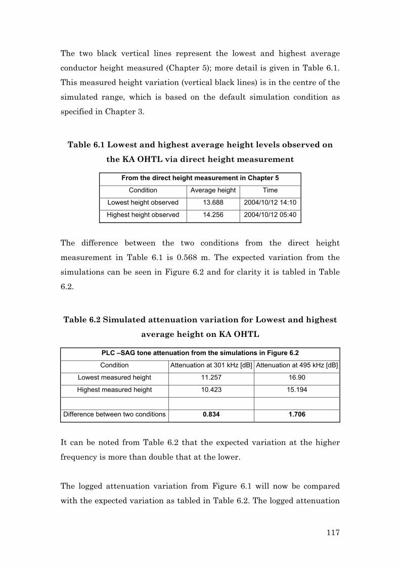
The two black vertical lines represent the lowest and highest average
conductor height measured (Chapter 5); more detail is given in Table 6.1.
This measured height variation (vertical black lines) is in the centre of the
simulated range, which is based on the default simulation condition as
specified in Chapter 3.
Table 6.1 Lowest and highest average height levels observed on
the KA OHTL via direct height measurement
From the direct height measurement in Chapter 5
Condition Average height Time
Lowest height observed 13.688 2004/10/12 14:10
Highest height observed 14.256 2004/10/12 05:40
The difference between the two conditions from the direct height
measurement in Table 6.1 is 0.568 m. The expected variation from the
simulations can be seen in Figure 6.2 and for clarity it is tabled in Table
6.2.
Table 6.2 Simulated attenuation variation for Lowest and highest
average height on KA OHTL
PLC –SAG tone attenuation from the simulations in Figure 6.2
Condition Attenuation at 301 kHz [dB] Attenuation at 495 kHz [dB]
Lowest measured height 11.257 16.90
Highest measured height 10.423 15.194
Difference between two conditions 0.834 1.706
It can be noted from Table 6.2 that the expected variation at the higher
frequency is more than double that at the lower.
The logged attenuation variation from Figure 6.1 will now be compared
with the expected variation as tabled in Table 6.2. The logged attenuation
117
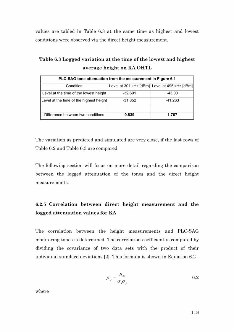
values are tabled in Table 6.3 at the same time as highest and lowest
conditions were observed via the direct height measurement.
Table 6.3 Logged variation at the time of the lowest and highest
average height on KA OHTL
PLC-SAG tone attenuation from the measurement in Figure 6.1
Condition Level at 301 kHz [dBm] Level at 495 kHz [dBm]
Level at the time of the lowest height -32.691 -43.03
Level at the time of the highest height -31.852 -41.263
Difference between two conditions 0.839 1.767
The variation as predicted and simulated are very close, if the last rows of
Table 6.2 and Table 6.3 are compared.
The following section will focus on more detail regarding the comparison
between the logged attenuation of the tones and the direct height
measurements.
6.2.5 Correlation between direct height measurement and the
logged attenuation values for KA
The correlation between the height measurements and PLC-SAG
monitoring tones is determined. The correlation coefficient is computed by
dividing the covariance of two data sets with the product of their
individual standard deviations [2]. This formula is shown in Equation 6.2
xyxy
x y
µρ
σ σ= 6.2
where
118
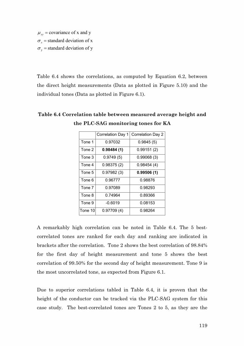
y
covariance of x and y
standard deviation of xstandard deviation of y
xy
x
µ
σσ
=
==
Table 6.4 shows the correlations, as computed by Equation 6.2, between
the direct height measurements (Data as plotted in Figure 5.10) and the
individual tones (Data as plotted in Figure 6.1).
Table 6.4 Correlation table between measured average height and
the PLC-SAG monitoring tones for KA
Correlation Day 1 Correlation Day 2
Tone 1 0.97032 0.9845 (5)
Tone 2 0.98484 (1) 0.99151 (2)
Tone 3 0.9749 (5) 0.99068 (3)
Tone 4 0.98375 (2) 0.98454 (4)
Tone 5 0.97982 (3) 0.99506 (1)
Tone 6 0.96777 0.98876
Tone 7 0.97089 0.98293
Tone 8 0.74964 0.89366
Tone 9 -0.6019 0.08153
Tone 10 0.97709 (4) 0.98264
A remarkably high correlation can be noted in Table 6.4. The 5 best-
correlated tones are ranked for each day and ranking are indicated in
brackets after the correlation. Tone 2 shows the best correlation of 98.84%
for the first day of height measurement and tone 5 shows the best
correlation of 99.50% for the second day of height measurement. Tone 9 is
the most uncorrelated tone, as expected from Figure 6.1.
Due to superior correlations tabled in Table 6.4, it is proven that the
height of the conductor can be tracked via the PLC-SAG system for this
case study. The best-correlated tones are Tones 2 to 5, as they are the
119

intersection of the two groups of best-correlated tones. Equation 6.3
formulates this more mathematically as:
6.3 1 2
( 2, 3, 4, 5) ( 2, 3, 4, 5, 10) ( 1, 2, 3, 4, 5)BestTones BestTonesDay BestTonesDayT T T T T T T T T T T T T T
= ∩= ∩
where
TN = Tone number N
Figure 6.3 is a magnification of Figure 6.1, which shows only the best-
correlated tones as identified by Equation 6.3.
Figure 6.3 Best correlated tones for KA PLC-SAG system
The average of best-correlated tones can be used to calibrate the PLC-SAG
system. This average will be referred to as the principal PLC-SAG tone.
The principal PLC-SAG tone is plotted in Figure 6.4 for same time
duration as the direct height measurement (Figure 5.10).
120

After the PLC-SAG system is calibrated, the direct height measurement
as shown in Figure 5.10 will be plotted on the same graph. But first, the
correlation between the direct height measurement and PLC-SAG
monitoring tones for the second case study will be analysed.
Figure 6.4 The principal PLC-SAG tones for the KA system
6.3 Case study 2 (Kriel-Tutuka) logged tones
6.3.1 Logged PLC-SAG monitoring tones
Figure 6.5 shows the logged levels of the ten PLC-SAG tones transmitted
from Tutuka Power Station and received at Kriel Power Station. A more
prominent day-night cycle is noticeable in the data.
121

Figure 6.5 Signal level variation of all ten tones on KT PLC-SAG
system. Measurement days 1 and 2 are indicated by the red
squares (Measured with Wandel & Goltermann selective
voltmeter)
The red square shows the part of the data that will be correlated with the
direct height measurement, similar to the previous case study. ‘Day 1’ in
the graph represents the first day of height measurements done on 4th
May 2004 and Day 2 presents the second day of height measurements
done on 6th May 2004.
6.3.2 General comments about the logged data
Two line outages occurred on 3rd and 4th May 2005, of which the author
was unaware until the direct height measurements had been performed.
The effects of the outage on the PLC system were prominent, since a step
change can be noted during those two days. It can also be noted that the
122

tones with lower frequencies are affected more than the tones with the
higher frequencies. Normally, when an outage occurs, an operator earths
the OHTL on the station side of the coupling equipment. This action
changes the impedance of the PLC system and, as a result, a step change
in the signal levels occurs. This does not affect the propagation
characteristics of the coupled signals and the PLC system is still
operational.
The data of 4th May 2004 had to be reconstructed, as the synchronized
direct height measurements were performed on that day. The best way to
reconstruct the data is to add a constant value during the time of the
outage to the affected regions. Appendix D shows the details of the tones
before and after reconstruction. Only five tones (Tones 3-6 and 9) could be
reconstructed successfully by following this unsophisticated approach.
6.3.3 Levels of the received PLC-SAG tones
The received level of the PLC-SAG tone 2 (Frequency = 320 kHz) varies
around -38.2 dBm (Figure 6.1).
According to the simulations in Chapter 3, the line attenuation at that
frequency is between 15 dB and 19 dB. The transmit level of the tone is
0.5 dBm at Tutuka Power Station. A 10 dB attenuator is used in this case
study (Chapter 4). Adding these losses together with the coupling losses
and losses associated with the measurement hybrid (similar to Equation
6.1) the expected attenuation can be computed to be between –34 dBm and
–38 dBm. The received level is not in the centre of the expected range, as
in the first case study, but it is close to the predicted range.
123

6.3.4 Variation of the received PLC-SAG tones compared to the
simulations
Tone 3 and Tone 9 were chosen for the analysis as they represent the 300
kHz and 475 kHz regions. The attenuation simulation done in Chapter 3
for the KT case study was re-plotted in Figure 6.6 for these two tones as a
function of average conductor height.
Figure 6.6 KT OHTL attenuation simulation as a function of
average conductor height for Tone 3 and Tone 10.
Details about the highest and lowest observed average conductor height
are tabled in Table 6.5 and are shown as vertical black lines in Figure 6.6.
It can be noted that the variation also occurred in the simulated region,
although the average height of the conductor is generally greater than
initially expected. It was confirmed with ESKOM that this transmission
124
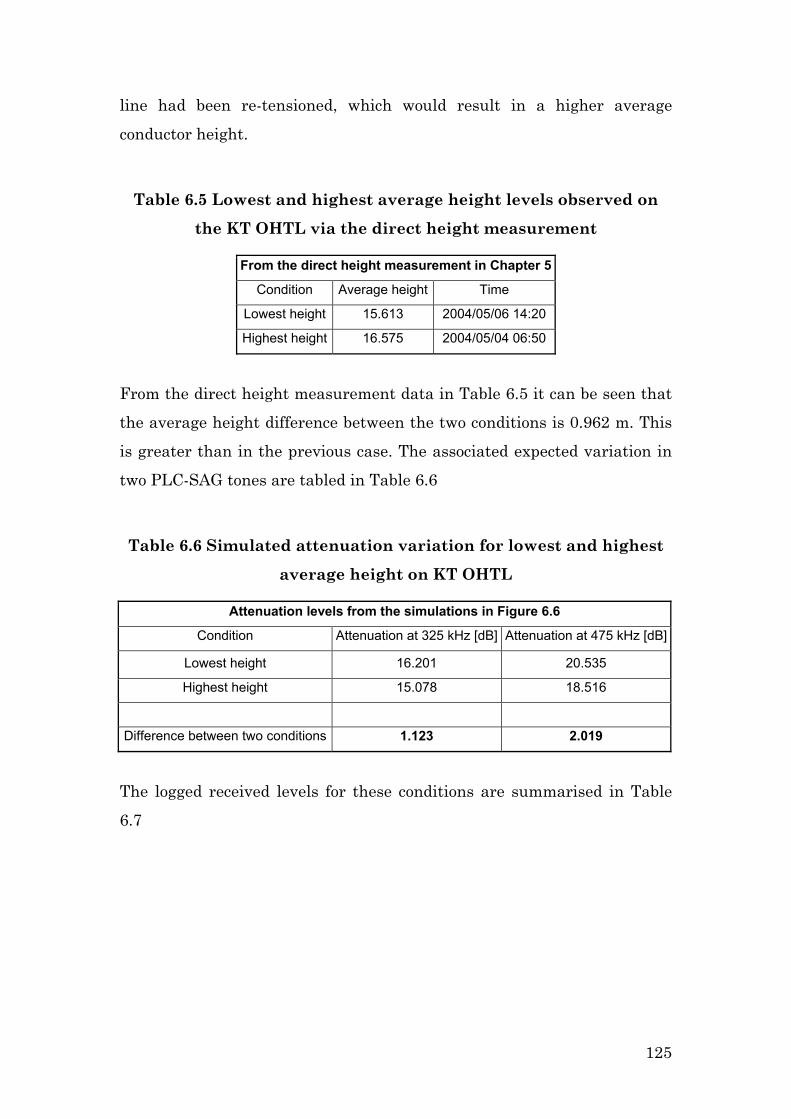
line had been re-tensioned, which would result in a higher average
conductor height.
Table 6.5 Lowest and highest average height levels observed on
the KT OHTL via the direct height measurement
From the direct height measurement in Chapter 5
Condition Average height Time
Lowest height 15.613 2004/05/06 14:20
Highest height 16.575 2004/05/04 06:50
From the direct height measurement data in Table 6.5 it can be seen that
the average height difference between the two conditions is 0.962 m. This
is greater than in the previous case. The associated expected variation in
two PLC-SAG tones are tabled in Table 6.6
Table 6.6 Simulated attenuation variation for lowest and highest
average height on KT OHTL
Attenuation levels from the simulations in Figure 6.6
Condition Attenuation at 325 kHz [dB] Attenuation at 475 kHz [dB]
Lowest height 16.201 20.535
Highest height 15.078 18.516
Difference between two conditions 1.123 2.019
The logged received levels for these conditions are summarised in Table
6.7
125
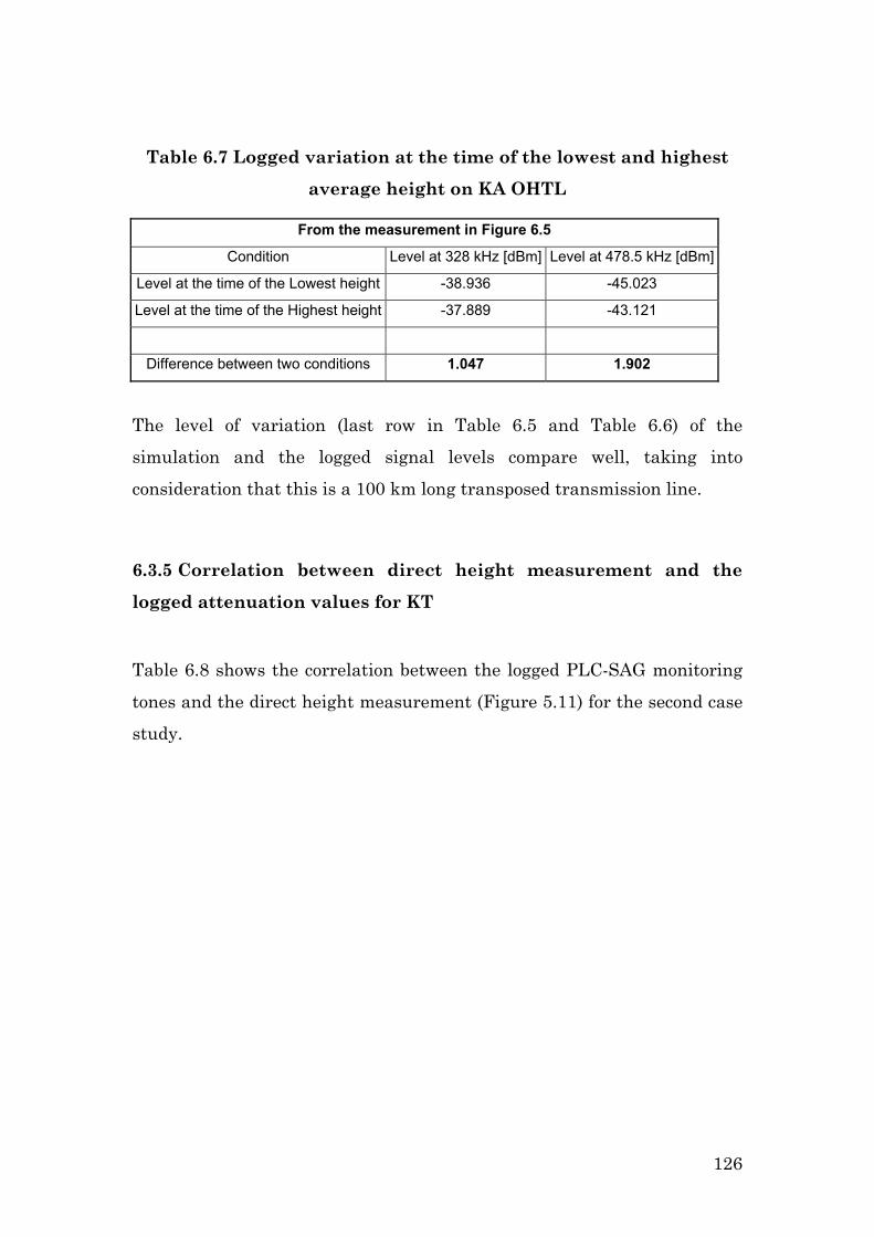
Table 6.7 Logged variation at the time of the lowest and highest
average height on KA OHTL
From the measurement in Figure 6.5
Condition Level at 328 kHz [dBm] Level at 478.5 kHz [dBm]
Level at the time of the Lowest height -38.936 -45.023
Level at the time of the Highest height -37.889 -43.121
Difference between two conditions 1.047 1.902
The level of variation (last row in Table 6.5 and Table 6.6) of the
simulation and the logged signal levels compare well, taking into
consideration that this is a 100 km long transposed transmission line.
6.3.5 Correlation between direct height measurement and the
logged attenuation values for KT
Table 6.8 shows the correlation between the logged PLC-SAG monitoring
tones and the direct height measurement (Figure 5.11) for the second case
study.
126
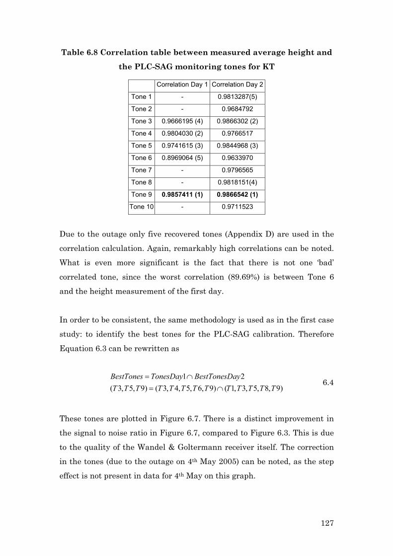
Table 6.8 Correlation table between measured average height and
the PLC-SAG monitoring tones for KT
Correlation Day 1 Correlation Day 2
Tone 1 - 0.9813287(5)
Tone 2 - 0.9684792
Tone 3 0.9666195 (4) 0.9866302 (2)
Tone 4 0.9804030 (2) 0.9766517
Tone 5 0.9741615 (3) 0.9844968 (3)
Tone 6 0.8969064 (5) 0.9633970
Tone 7 - 0.9796565
Tone 8 - 0.9818151(4)
Tone 9 0.9857411 (1) 0.9866542 (1)
Tone 10 - 0.9711523
Due to the outage only five recovered tones (Appendix D) are used in the
correlation calculation. Again, remarkably high correlations can be noted.
What is even more significant is the fact that there is not one ‘bad’
correlated tone, since the worst correlation (89.69%) is between Tone 6
and the height measurement of the first day.
In order to be consistent, the same methodology is used as in the first case
study: to identify the best tones for the PLC-SAG calibration. Therefore
Equation 6.3 can be rewritten as
6.4 1 2
( 3, 5, 9) ( 3, 4, 5, 6, 9) ( 1, 3, 5, 8, 9)BestTones TonesDay BestTonesDayT T T T T T T T T T T T T
= ∩= ∩
These tones are plotted in Figure 6.7. There is a distinct improvement in
the signal to noise ratio in Figure 6.7, compared to Figure 6.3. This is due
to the quality of the Wandel & Goltermann receiver itself. The correction
in the tones (due to the outage on 4th May 2005) can be noted, as the step
effect is not present in data for 4th May on this graph.
127
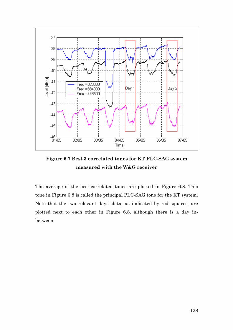
Figure 6.7 Best 3 correlated tones for KT PLC-SAG system
measured with the W&G receiver
The average of the best-correlated tones are plotted in Figure 6.8. This
tone in Figure 6.8 is called the principal PLC-SAG tone for the KT system.
Note that the two relevant days’ data, as indicated by red squares, are
plotted next to each other in Figure 6.8, although there is a day in-
between.
128

Figure 6.8 The principal PLC-SAG tone for KT (Average of the 3
best correlated KT PLC-SAG tones)
The data represented in Figure 6.4 and Figure 6.8 will be used in the
following section to calibrate the PLC-SAG system for the two case
studies.
6.4 Calibration of the PLC-SAG system
The goal of the calibration is to transform the level of the PLC-SAG
monitoring tones (which is in dBm) into the average conductor height of
the transmission line (which is in meters). Theoretical transfer curves
(Figure 6.2 and Figure 6.6), which relate the average conductor height and
signal attenuation, can be used as a lookup table to utilize a calibration
function.
129

More specifically, the average of the best-correlated tones (called the
principal PLC-SAG tone as shown in Figure 6.4 and Figure 6.8) will be
calibrated to compare it with the measured average height of the two case
studies.
6.4.1 Case study 1 (Koeberg-Acacia)
The theoretical relationship between average height and signal
attenuation is computed by using the simulation program. The principal
PLC-SAG tone for KA was identified in Section 6.2.5 as the combination of
Tones 2,3,4 and 5. The theoretical transfer function for the principal PLC-
SAG tone is plotted in Figure 6.9 as the red stars. All the signal losses as
specified in Equation 6.1 are included in the presented simulation. It can
also be noted that the axes are differently defined - to compute the
Average height for a given signal level.
Figure 6.9 Theoretical calibration curve for the principal PLC-
SAG tone for the KA OHTL.
130

Two additional functions were also plotted on Figure 6.9 together with the
simulated data, a normal line and a more complex function, on Figure 6.9.
A Least Squares based curve-fitting algorithm called (‘polyfit’) from
Matlab was used to characterize the two functions. The specific functions
as plotted in Figure 6.9 can be described by the following parameters:
The line:
y mx c= + 6.5
where
m = 0.710 ( The slope)
c = 35.544 ( Offset value)
The more complex function:
a by e x= 6.6
where
a = 7.96 + 4.902i
b = -1.56
By studying Figure 6.9 it can be noted that in the framework of the
simulated range, the complex function best fits the data, especially at
12.25 m and 15.75 m. For the range between 13.7 m and 14.3 m there is a
small difference between the two curves. Therefore, from the theory, one
expects linear behaviour in the region of the measured height variation.
This is remarkable, since this implies that the principal PLC-SAG tone
can be calibrated in the required region by using a linear transformation.
The two data sets, namely the height measurement for two days (Figure
5.10) and the average of the best-correlated PLC-SAG tones (Figure 6.4),
will now be incorporated to compute the empirical calibration curve in the
form of a straight line (Equation 6.5). To get the best parameters for
131
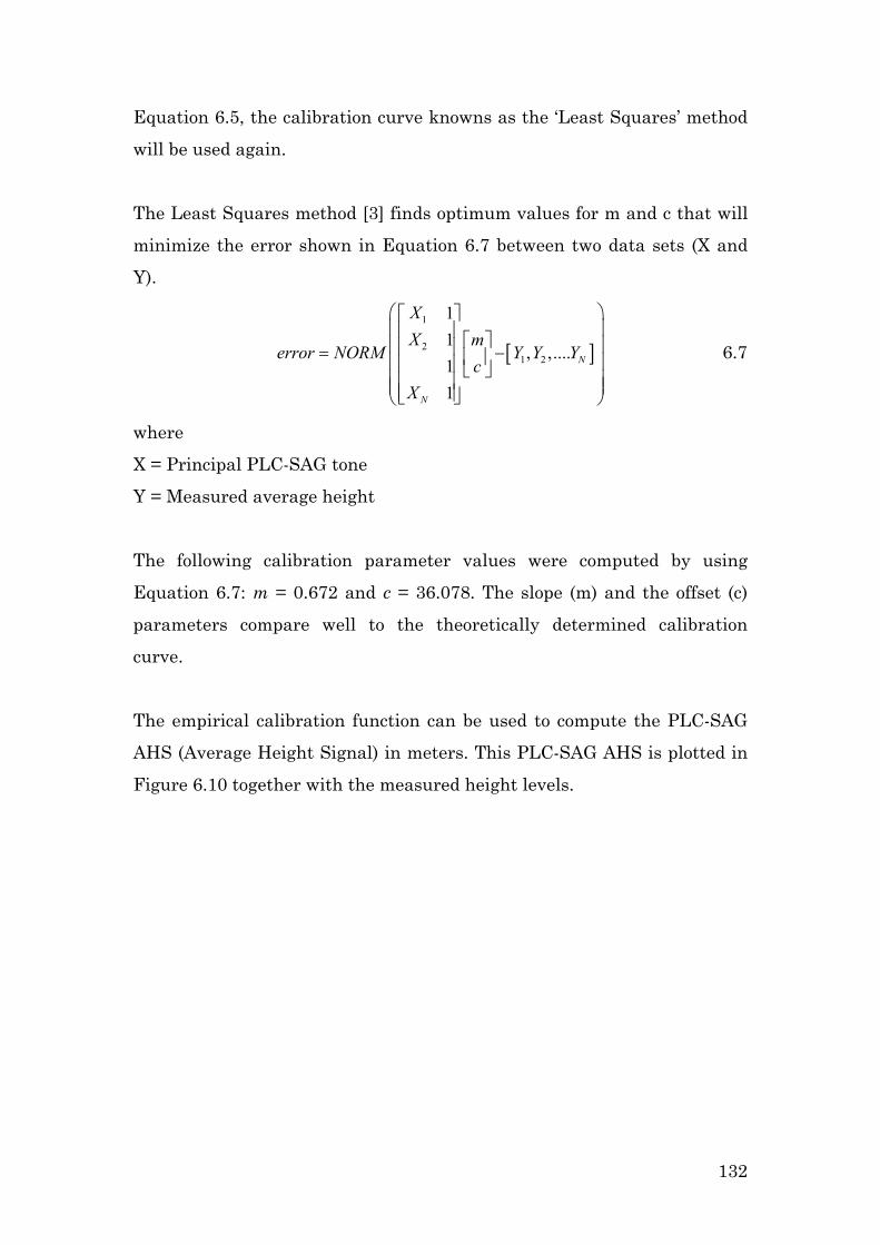
Equation 6.5, the calibration curve knowns as the ‘Least Squares’ method
will be used again.
The Least Squares method [3] finds optimum values for m and c that will
minimize the error shown in Equation 6.7 between two data sets (X and
Y).
6.7 [
1
21 2
11
, ,....11
N
N
XX m
error NORM Y Y Yc
X
= −
]
where
X = Principal PLC-SAG tone
Y = Measured average height
The following calibration parameter values were computed by using
Equation 6.7: m = 0.672 and c = 36.078. The slope (m) and the offset (c)
parameters compare well to the theoretically determined calibration
curve.
The empirical calibration function can be used to compute the PLC-SAG
AHS (Average Height Signal) in meters. This PLC-SAG AHS is plotted in
Figure 6.10 together with the measured height levels.
132

00:00 06:00 12:00 18:00 00:00 06:00 12:00 18:00 00:0013.6
13.7
13.8
13.9
14
14.1
14.2
14.3
Time
Hei
ght v
aria
tion
[m] /
Cal
ibra
ted
PLC
-SA
G le
vel [
dBm
]
Average conductor height variationAverage of the Best PLC SAG Monitoring tones
2004/10/05 2004/10/12
Figure 6.10 Calibrated PLC-SAG signal and the measured average
height of the conductor for KA (Correlation = 99.02%)
The two data sets, presented in Figure 6.10, have a correlation of 99.02 %.
This is a truly an outstanding result. Very small errors between the data
sets can be noted, which are much smaller than 75 mm. It can be noted
that, according to Eskom specialists, an error of up to 500 mm is
commonly allowable for this type of conductor height tracking system.
From a different viewpoint, Figure 6.10 shows a PLC-SAG AHS, which
presents the average height of the whole OHTL by utilising the existing
PLC infrastructure in an innovative way. The measured average height
obtained (by monitoring three spans) correlates nearly perfectly with the
PLC-SAG AHS. This is without doubt proof that very accurate height
measurement can be done via the PLC-SAG system.
The calibration of case study two (KT OHTL) will now be discussed.
133
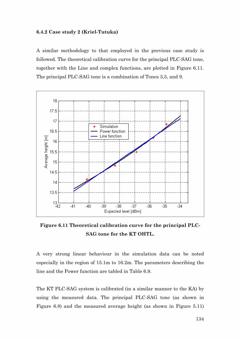
6.4.2 Case study 2 (Kriel-Tutuka)
A similar methodology to that employed in the previous case study is
followed. The theoretical calibration curve for the principal PLC-SAG tone,
together with the Line and complex functions, are plotted in Figure 6.11.
The principal PLC-SAG tone is a combination of Tones 3,5, and 9.
Figure 6.11 Theoretical calibration curve for the principal PLC-
SAG tone for the KT OHTL.
A very strong linear behaviour in the simulation data can be noted
especially in the region of 15.1m to 16.2m. The parameters describing the
line and the Power function are tabled in Table 6.9.
The KT PLC-SAG system is calibrated (in a similar manner to the KA) by
using the measured data. The principal PLC-SAG tone (as shown in
Figure 6.8) and the measured average height (as shown in Figure 5.11)
134
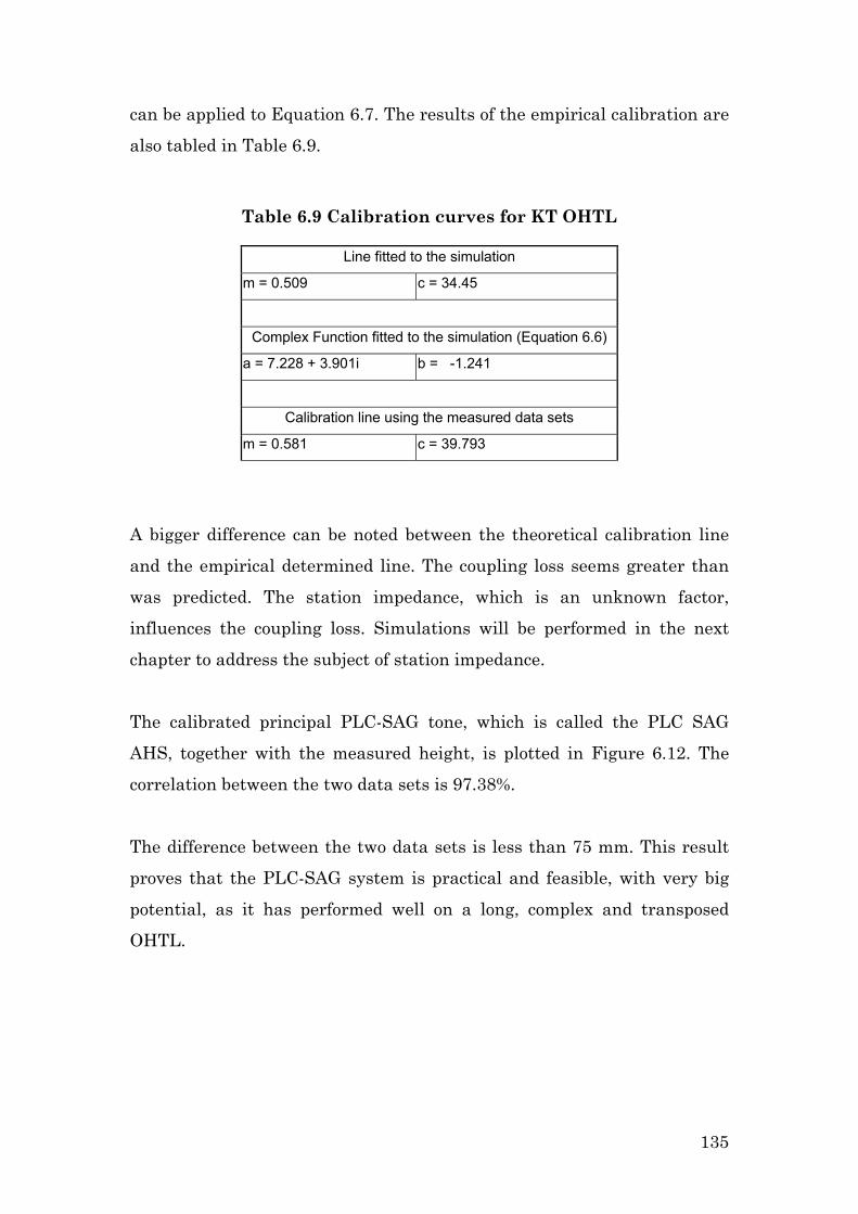
can be applied to Equation 6.7. The results of the empirical calibration are
also tabled in Table 6.9.
Table 6.9 Calibration curves for KT OHTL
Line fitted to the simulation
m = 0.509 c = 34.45
Complex Function fitted to the simulation (Equation 6.6)
a = 7.228 + 3.901i b = -1.241
Calibration line using the measured data sets
m = 0.581 c = 39.793
A bigger difference can be noted between the theoretical calibration line
and the empirical determined line. The coupling loss seems greater than
was predicted. The station impedance, which is an unknown factor,
influences the coupling loss. Simulations will be performed in the next
chapter to address the subject of station impedance.
The calibrated principal PLC-SAG tone, which is called the PLC SAG
AHS, together with the measured height, is plotted in Figure 6.12. The
correlation between the two data sets is 97.38%.
The difference between the two data sets is less than 75 mm. This result
proves that the PLC-SAG system is practical and feasible, with very big
potential, as it has performed well on a long, complex and transposed
OHTL.
135

00:00 06:00 12:00 18:00 00:00 06:00 12:00 18:00 00:0015.6
15.8
16
16.2
16.4
16.6
16.8
Time
Hei
ght v
aria
tion
[m] /
Cal
ibra
ted
PLC
-SA
G le
vel [
dBm
] Average conductor height variationAverage of 3 Best PLC SAG Monitoring tones
2004/05/04 2004/05/06
Figure 6.12 PLC-SAG AHS and the measured average height of the
conductor (Correlation = 97,38%) for KT
6.5 Conclusions
The computations in this chapter have proved that the average height of
an OHTL conductor could be tracked via a PLC-SAG system exceptionally
accurately to within 75 mm on a day-to-day time scale.
The average height of an OHTL conductor can be tracked accurately on a
day-to-day time scale. But how stable is the PLC-SAG system over longer
periods of time? This question will be addressed in the following chapter.
136

References:
[1] De Villiers, W., Prediction and measurement of Power Line Carrier
signal attenuation and fluctuation, MScEng Thesis, University of
Stellenbosch, November 2001.
[2] R.E. Ziemer and W.H. Tranter, Principles of Communications,
Fourth Edition, John Wiley & Sons, 1988.
[3] J.G. Proakis and D.G. Manolakis, Digital signal processing
principles, algorithms and applications, Third Edition. Prentice-hall
international, 1996.
137

Chapter 7
PLC-SAG impedance monitoring system
7.1 Introduction
A strong relationship between the average conductor height and the PLC-
SAG tone level was documented in the previous chapter. This phenomenon
seemed very stable in the timeframe of the experiments. The data
produced from the installations were analysed to see whether any other
events or phenomena in the system would have an impact on the PLC-
SAG method.
Logged data were studied and an unexpected step change was seen to
occur in the received levels of the PLC-SAG monitoring tones. Initially,
this effect was not alarming, but after analysis it became apparent that it
is indeed problematic for the PLC-SAG system. An explanation is given in
Section 7.2 regarding this PLC-SAG monitoring tone step effect and the
associated implications.
An innovative and practical solution was discovered during the process of
solving the PLC-SAG step problem, which primarily involves a PLC
hybrid (Chapter 2 and Chapter 4). In order to fully understand the
proposed solution, the theory of a hybrid will be disused in more depth in
Section 7.3. In Section 7.4 the isolation of the hybrid is discussed and the
fact that it was discovered that the hybrid could be utilised as a complex
impedance-monitoring device. By monitoring the complex impedance of
138
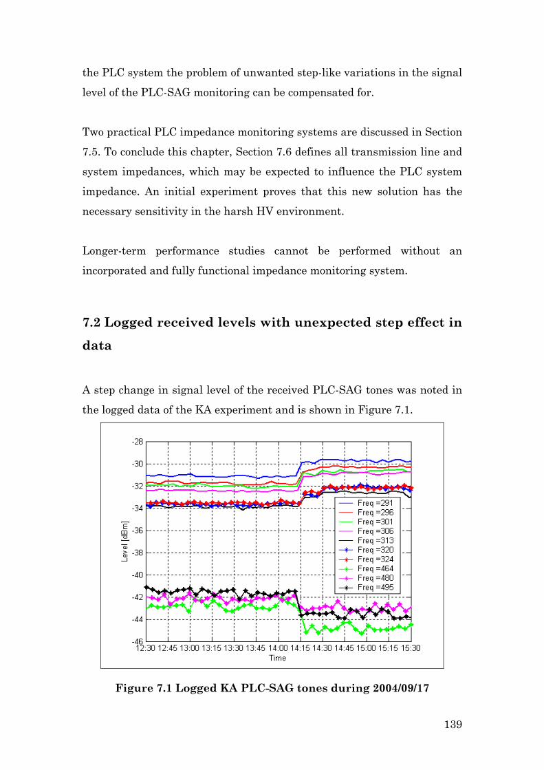
the PLC system the problem of unwanted step-like variations in the signal
level of the PLC-SAG monitoring can be compensated for.
Two practical PLC impedance monitoring systems are discussed in Section
7.5. To conclude this chapter, Section 7.6 defines all transmission line and
system impedances, which may be expected to influence the PLC system
impedance. An initial experiment proves that this new solution has the
necessary sensitivity in the harsh HV environment.
Longer-term performance studies cannot be performed without an
incorporated and fully functional impedance monitoring system.
7.2 Logged received levels with unexpected step effect in
data
A step change in signal level of the received PLC-SAG tones was noted in
the logged data of the KA experiment and is shown in Figure 7.1.
Figure 7.1 Logged KA PLC-SAG tones during 2004/09/17
139
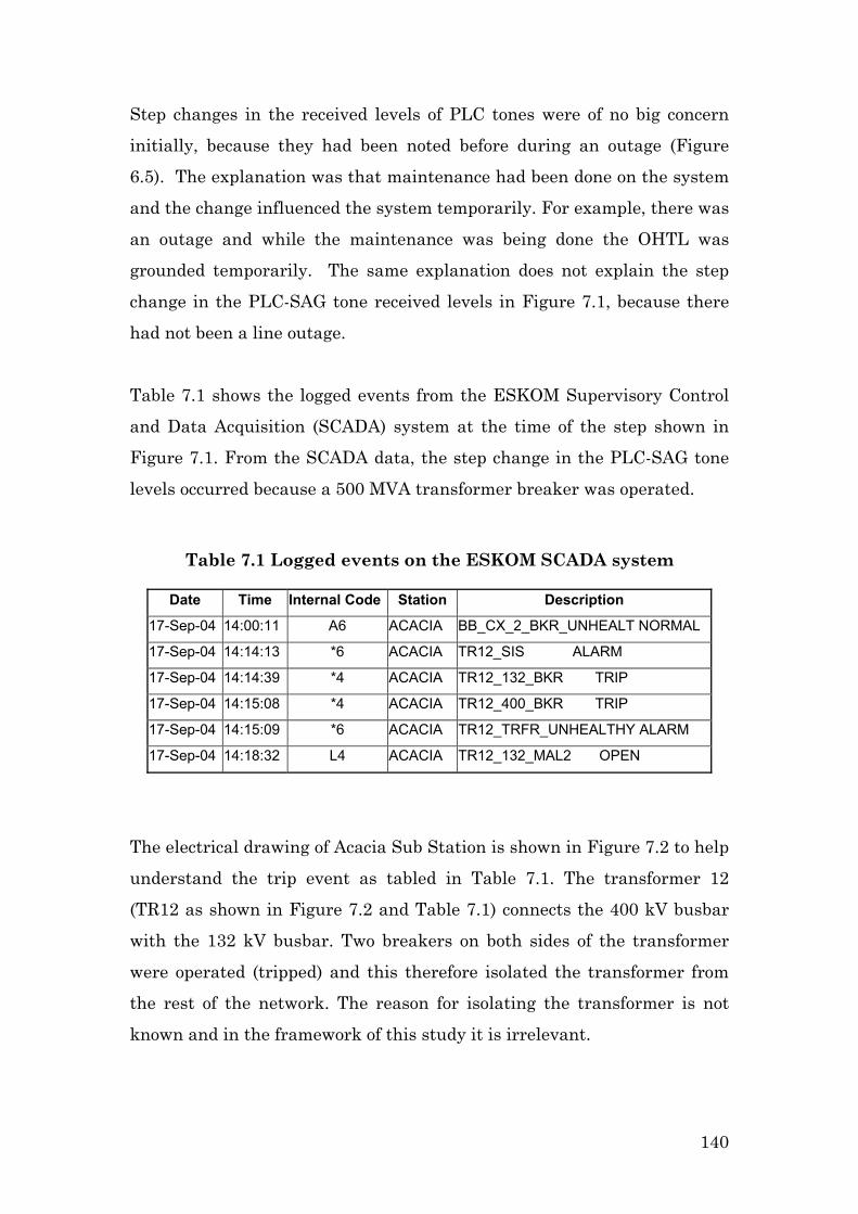
Step changes in the received levels of PLC tones were of no big concern
initially, because they had been noted before during an outage (Figure
6.5). The explanation was that maintenance had been done on the system
and the change influenced the system temporarily. For example, there was
an outage and while the maintenance was being done the OHTL was
grounded temporarily. The same explanation does not explain the step
change in the PLC-SAG tone received levels in Figure 7.1, because there
had not been a line outage.
Table 7.1 shows the logged events from the ESKOM Supervisory Control
and Data Acquisition (SCADA) system at the time of the step shown in
Figure 7.1. From the SCADA data, the step change in the PLC-SAG tone
levels occurred because a 500 MVA transformer breaker was operated.
Table 7.1 Logged events on the ESKOM SCADA system
Date Time Internal Code Station Description
17-Sep-04 14:00:11 A6 ACACIA BB_CX_2_BKR_UNHEALT NORMAL
17-Sep-04 14:14:13 *6 ACACIA TR12_SIS ALARM
17-Sep-04 14:14:39 *4 ACACIA TR12_132_BKR TRIP
17-Sep-04 14:15:08 *4 ACACIA TR12_400_BKR TRIP
17-Sep-04 14:15:09 *6 ACACIA TR12_TRFR_UNHEALTHY ALARM
17-Sep-04 14:18:32 L4 ACACIA TR12_132_MAL2 OPEN
The electrical drawing of Acacia Sub Station is shown in Figure 7.2 to help
understand the trip event as tabled in Table 7.1. The transformer 12
(TR12 as shown in Figure 7.2 and Table 7.1) connects the 400 kV busbar
with the 132 kV busbar. Two breakers on both sides of the transformer
were operated (tripped) and this therefore isolated the transformer from
the rest of the network. The reason for isolating the transformer is not
known and in the framework of this study it is irrelevant.
140

Figure 7.2 Simplistic electrical diagram showing the two 500 MVA
transformers at Acacia Sub Station
The influences of this transformer isolation event on the PLC system will
now be discussed. The power network change resulted in a station
impedance change at PLC frequencies. The Line Trap’s (LT) function is to
minimize the effect of the station impedance variation on the PLC system
(Chapter 2). Ideally, the LT totally isolates the PLC system from the
station impedance variations. Simulations need to be performed to
quantify the level of isolation which a non-ideal LT actually provides. The
discovered step effect in Figure 7.1 could be due to a faulty line trap or it
could be within the realistic performance expectation of a fully functional
LT.
In previous simulations, shown in Chapter 2 and 3, a value of 1000 Ω was
used for the station impedance ( sZ ) due to the lack of more detailed
information. Using the simulation program as described in Chapter 2 the
effect of station impedance ( sZ ) variations on the PLC signal attenuation
was simulated. The result of the simulations is shown in Figure 7.3.
141
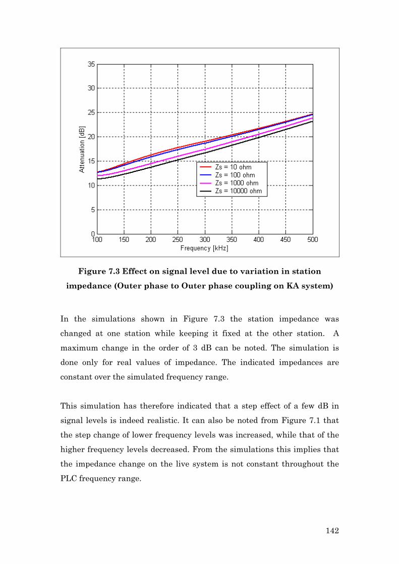
Figure 7.3 Effect on signal level due to variation in station
impedance (Outer phase to Outer phase coupling on KA system)
In the simulations shown in Figure 7.3 the station impedance was
changed at one station while keeping it fixed at the other station. A
maximum change in the order of 3 dB can be noted. The simulation is
done only for real values of impedance. The indicated impedances are
constant over the simulated frequency range.
This simulation has therefore indicated that a step effect of a few dB in
signal levels is indeed realistic. It can also be noted from Figure 7.1 that
the step change of lower frequency levels was increased, while that of the
higher frequency levels decreased. From the simulations this implies that
the impedance change on the live system is not constant throughout the
PLC frequency range.
142

The operational PLC system is built to be fully functioning in the event of
station impedance changes. The PLC-SAG system, on the other hand,
needs to be calibrated very accurately and a step change (as noted in
Figure 7.1) would result in incorrect height monitoring levels.
This was very quickly singled out as the biggest problem that needed to be
overcome to make the PLC-SAG system robust and practical.
An innovative solution was found to address this problem. In order to
understand the proposed solution, the characteristics of the hybrid will be
discussed in the following section.
7.3 Background theory of hybrid applied to the PLC
System
In [1] a similar hybrid to that used by the PLC system is used in a vacuum
tube amplifier. The equations and theory that relate directly to the hybrid
itself in this section are similar to those in [1], but as applied to the PLC
system. Figure 7.4 shows an electrical circuit of a hybrid or specially
configured two-winding transformer. When driven at Port 1, as depicted, a
properly designed hybrid serves as a differential mode power splitter.
Z_match Z2
Z3
+
-
V1
Hybrid
Z1
Port 1 Port 2
Port 3
e
f
a
c
b
d
AC
Figure 7.4 Circuit diagram of a hybrid
143
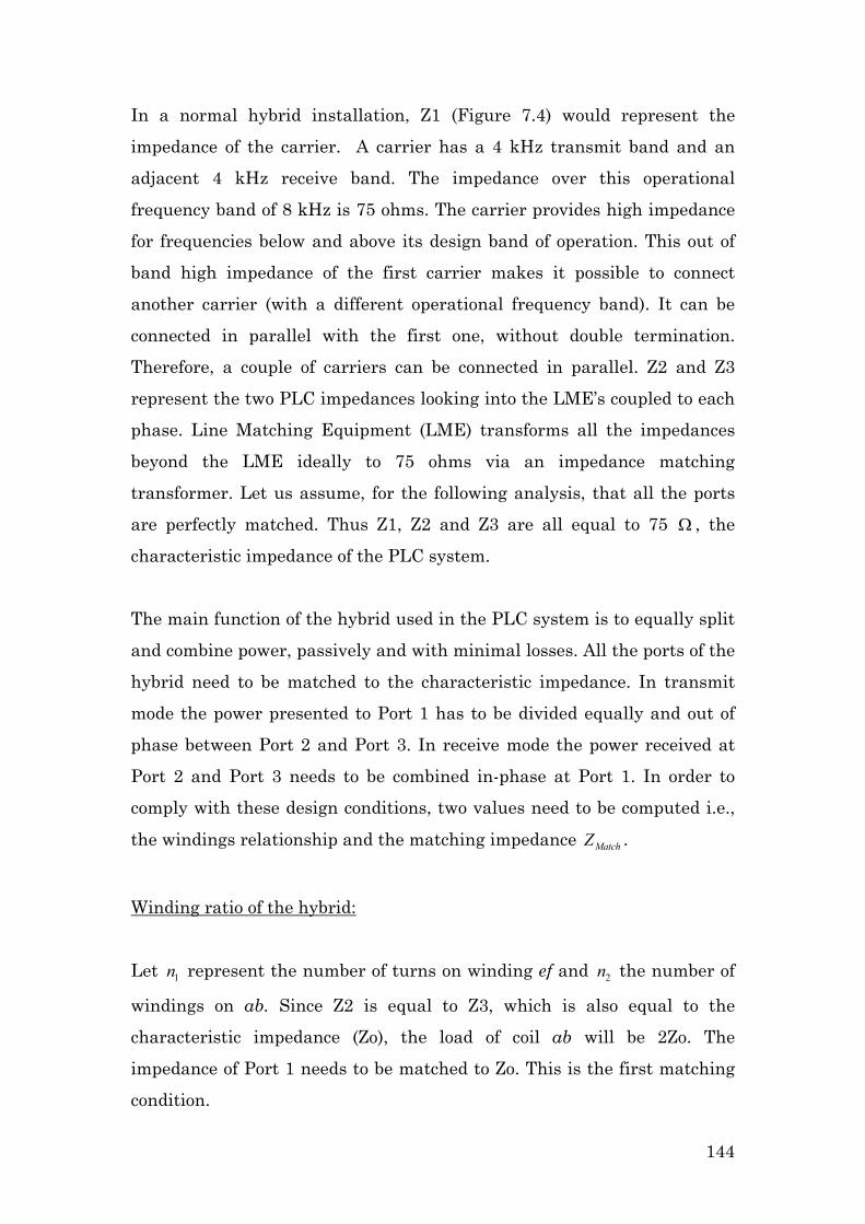
In a normal hybrid installation, Z1 (Figure 7.4) would represent the
impedance of the carrier. A carrier has a 4 kHz transmit band and an
adjacent 4 kHz receive band. The impedance over this operational
frequency band of 8 kHz is 75 ohms. The carrier provides high impedance
for frequencies below and above its design band of operation. This out of
band high impedance of the first carrier makes it possible to connect
another carrier (with a different operational frequency band). It can be
connected in parallel with the first one, without double termination.
Therefore, a couple of carriers can be connected in parallel. Z2 and Z3
represent the two PLC impedances looking into the LME’s coupled to each
phase. Line Matching Equipment (LME) transforms all the impedances
beyond the LME ideally to 75 ohms via an impedance matching
transformer. Let us assume, for the following analysis, that all the ports
are perfectly matched. Thus Z1, Z2 and Z3 are all equal to 75 Ω , the
characteristic impedance of the PLC system.
The main function of the hybrid used in the PLC system is to equally split
and combine power, passively and with minimal losses. All the ports of the
hybrid need to be matched to the characteristic impedance. In transmit
mode the power presented to Port 1 has to be divided equally and out of
phase between Port 2 and Port 3. In receive mode the power received at
Port 2 and Port 3 needs to be combined in-phase at Port 1. In order to
comply with these design conditions, two values need to be computed i.e.,
the windings relationship and the matching impedance MatchZ .
Winding ratio of the hybrid:
Let represent the number of turns on winding ef and the number of
windings on ab. Since Z2 is equal to Z3, which is also equal to the
characteristic impedance (Zo), the load of coil ab will be 2Zo. The
impedance of Port 1 needs to be matched to Zo. This is the first matching
condition.
1n 2n
144

2
11 0
2
2n0Z Z Z
n
= =
7.1
Equation 7.1 can now be rewritten in terms of the winding ratio, as
Equation 7.2 shows
01
2 0
12 2Zn
n Z= = 7.2
The hybrid is made in such way that the number of turns on coil ac is
equal to the number of turns on coil cb, the summation of which is equal to
(number of turns for coil ab). 2n
Common hybrid impedance:
Now assume that Port 2 is driven by a generator with impedance Zo and
that Ports 1 and 3 are passively terminated also with Zo.
The impedance of Port 2 or adZ can be formulated in general as:
( )3
3
Match cbad ac
Match cb
Z Z ZZ Z
Z Z Z+
= ++ +
7.3
Assume next that Port 3 is isolated. Thus V = 0, and ab 3Z is effectively
disconnected. Thus Equation 7.3 reduces to Equation 7.4. This is the
isolation condition.
ad ac MatxhZ Z Z= + 7.4
But adZ needs to be equal to 0Z , with Port 1 correctly terminated, acZ can
be computed as follows in Equation 7.5.
145

22 2
020 0
1 1
124 2ac
nZnZ Z Z
n n
= =
= 7.5
By substituting Equation 7.5 into Equation 7.4 with adZ = Zo, MatchZ can be
computed to be 0
2Z
.
The current flowing in coil ac (in an ideal transformer) would produce a
voltage in coil cb that would be equal to the voltage produced in coil ac.
Thus
ac cbV V= 7.6
but, with Port 1 terminated in Zo
ac cdV V= 7.7
Therefore, the voltage between b and d (or at Port 3) will be zero. In fact
it makes no difference if 3Z is connected or not and our assumption that 3Z
is disconnected does not have an impact on the deduction made [1].
7.4 Isolation of a hybrid
The following section will extend the theoretical discussion of a hybrid.
The analysis, as discussed from this point onwards, is unique in the
framework of PLC system impedances and the monitoring thereof.
In Subsection 7.4.1 the isolation between Port 2 and Port 3 of the hybrid
will be examined. The isolation characteristics are then further explored
146

via simulations (Subsection 7.4.2) and a laboratory experiment
(Subsection 7.4.3).
7.4.1 Isolation
The isolation between Port 2 and Port 3 will now be discussed. Assume
Port 2 is driven by a generator gV with impedance Zo and Port 3 is
terminated in Zo. Then isolation between the two ports can be defined in
Equation 7.8 as:
20log ad
db
VIsolationV
= 7.8
From the previous analysis, it has become clear that if the hybrid is
correctly terminated in Zo at all three ports, the isolation is perfect, in the
ideal case. The reason for this ideal isolation is due to zero voltage at Port
3, as previously discussed.
Let us assume that we do not know the value of the impedance at Port 1.
The isolation can be defined as a function of 1Z .
The voltage relationship of Port 2 and Port 3 can be expressed as:
0
0 1
3ad
db
V Z ZV Z Z
1+=
− 7.9
An odd mode excitation (Figure 7.5) and even mode excitation (Figure 7.6)
analysis can be done to derive Equation 7.9 [2]. All the currents and
voltages for the two modes can be derived and then superimposed to
obtain Equation 7.9. A key assumption is that the transformer is ideal.
147

Z_match
Zo
Zo
+
-
V1
Hybrid
Z1
Port 1
Port 2
Port 3
e
f
a
c
b
d
AC
AC
+
-
+-
+Vg/2
+Vg/2
Figure 7.5 Odd mode excitation of hybrid
Z_match
Zo
Zo
+
-
V1
Hybrid
Z1
Port 1
Port 2
Port 3
e
f
a
c
b
d
AC
AC
+
-
-
+
+Vg/2
+Vg/2
Figure 7.6 Even mode excitation of hybrid
For this specific hybrid we know that the characteristic impedance (Zo) is
equal to 75 . The isolation, as defined in Equation 7.8, can then be
defined as:
Ω
1
1
75 320log75
ZIsolationZ
+=
− 7.10
with 1Z an arbitrary complex impedance connected to Port 1.
148
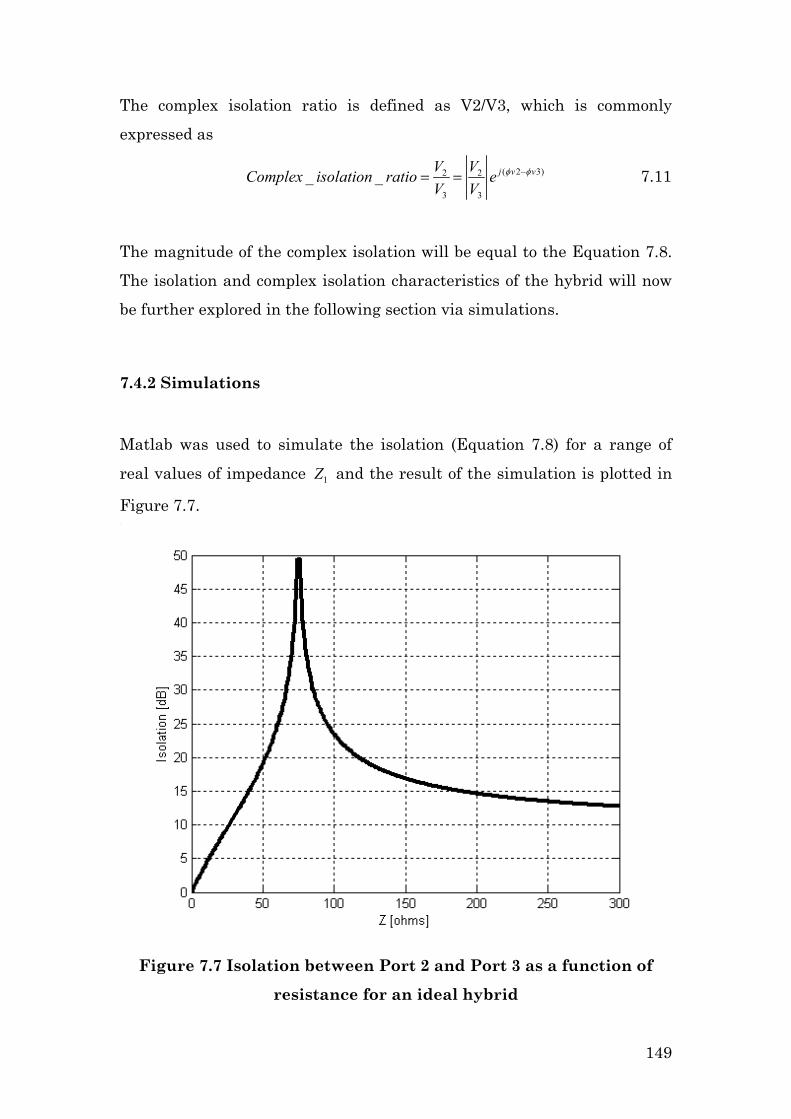
The complex isolation ratio is defined as V2/V3, which is commonly
expressed as
( 2 3)2 2
3 3
_ _ j v vV VComplex isolation ratio eV V
φ φ−= = 7.11
The magnitude of the complex isolation will be equal to the Equation 7.8.
The isolation and complex isolation characteristics of the hybrid will now
be further explored in the following section via simulations.
7.4.2 Simulations
Matlab was used to simulate the isolation (Equation 7.8) for a range of
real values of impedance 1Z and the result of the simulation is plotted in
Figure 7.7.
Figure 7.7 Isolation between Port 2 and Port 3 as a function of
resistance for an ideal hybrid
149

From Figure 7.7, it may be seen that the isolation tends towards infinity
when the impedance at Port 1 (Z1) is close to 75 ohms. It can also be noted
that the change in isolation increases as the value of resistance
approaches 75 ohm from both sides. Therefore, even if the isolation could
be measured, the value of resistance cannot be determined uniquely. The
complex isolation will now be discussed.
The real part of the complex isolation is plotted in Figure 7.8 and the
imaginary part in Figure 7.9. By studying the graphs in these figures, it is
clearly evident that the complex isolation changes rapidly as the
impedance at Port 1 approaches 75 Ω . If the real part of the complex
isolation could be measured, together with the imaginary part, then the
complex impedance could be uniquely determined.
Figure 7.8 Real part of the complex isolation for a complex Z1 for
an ideal hybrid
150

Figure 7.9 Imaginary part of the complex isolation for a complex
Z1 for an ideal hybrid
7.4.3 Insertion loss laboratory experiment
A laboratory experiment was performed to verify the simulations and
theory.
A hybrid, type A9BM manufactured by ABB Powertech [3], was used to
perform the experiment. Photograph 4.1 depicts this type of Hybrid, which
is commonly used in ESKOM PLC systems.
Port 2 of the hybrid was driven by a Wandel & Goltermann signal
generator (PS-3), configured with a 75 Ω output impedance. A Tektronix
TDS 220 oscilloscope was connected to Port 3 and Port 2, while port 3 is
terminated in 75 Ω . This experiment was done at 250 kHz. Different
resistors were then applied to Port 1 and the isolation was measured
151

between Port 2 and Port 3 via the oscilloscope. The result of the
experiment, together with the simulated graph, is plotted in Figure 7.10.
Figure 7.10 Experimental results and simulations of isolation for
different values of resistance at Port 1 at 250 kHz. The exact
resistance values are 17.7, 47.7, 67, 74.3, 81.15, 98.4, 149 and 270
ohms as measured on a bridge.
The black graph represents a simulation for the ideal case, as shown in
Figure 7.7. The red asterisks show the measured values. The experiment
indicates that the simulation model and the measurements correlate well
for a wide range of resistance values. When Port 1 is open-circuited the
simulated value is 9.5 dB and measurement value is 9.71 dB (Not shown
in Figure 7.10). The measured isolation for the 74.7 Ω resistor is lower
than the simulated value because the noise floor of the oscilloscope limits
the measurement accuracy.
152

7.5 PLC impedance (PLC-IMP) monitoring system
From the isolation analysis in Section 7.4 it became clear that the hybrid
could be used to measure the impedance at Port 1 near 75 . In practice
when performing such a measurement Port 2 and Port 3 need to be well
terminated. The hybrid needs to be driven at either Port 2 or Port 3 and
the complex ratio between Port 2 and Port 3 needs to be measured very
accurately to determine the complex impedance at Port 1. The impedance
measurement technique is only sensitive at impedances close to 75 Ω .
Ω
All the conditions mentioned appear to be reachable, with the goal of
realizing an impedance measurement system in the current PLC-SAG
hybrid setup (Chapter 4) without any additional hardware change to the
current PLC system attained. This is truly exceptional. The technique
described here is distinct from the usual impedance bridge technique used
in the PLC environment, as described in [4]. The new technique is called
PLC-IMP.
Two potential PLC impedance measurement setups will now be discussed.
The first setup will enable measurement of the PLC-system impedances at
carrier frequencies. The second measurement setup will address PLC-SAG
tone impedance measurements.
7.5.1 Monitoring the PLC impedance at the carrier frequency
By inserting a Measurement Hybrid between Port 3 of the existing hybrid
and the LMU the phase impedance of the PLC system can be monitored in
real-time. This is exactly the same hybrid configuration as discussed in
Chapter 4. The impact of the measurement hybrid on the existing PLC
system is therefore the same as discussed in Chapter 4.
153
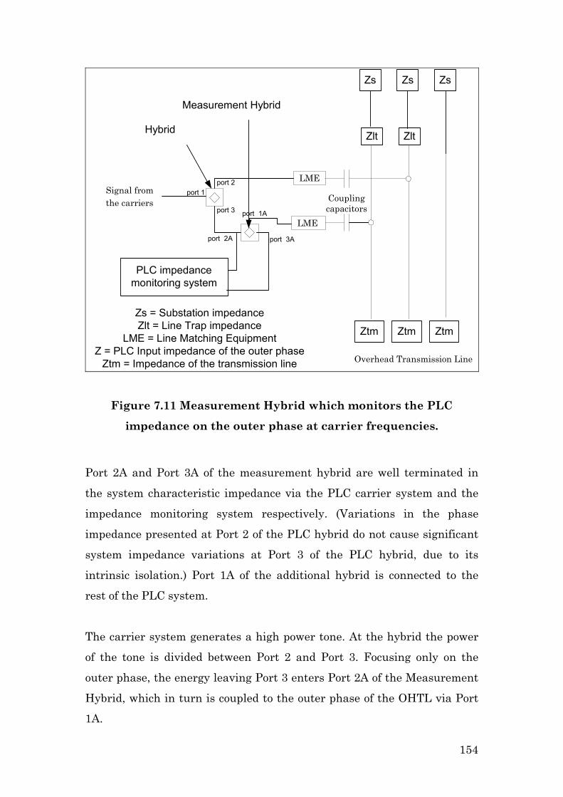
Overhead Transmission Line
LME
Couplingcapacitors
Signal fromthe carriers
Zs Zs Zs
Zlt
LME
Zs = Substation impedanceZlt = Line Trap impedance
LME = Line Matching EquipmentZ = PLC Input impedance of the outer phase
Ztm = Impedance of the transmission line
PLC impedancemonitoring system
port 2
port 3
port 1
Ztm Ztm Ztm
port 1A
port 2A port 3A
Hybrid
Measurement Hybrid
Zlt
Figure 7.11 Measurement Hybrid which monitors the PLC
impedance on the outer phase at carrier frequencies.
Port 2A and Port 3A of the measurement hybrid are well terminated in
the system characteristic impedance via the PLC carrier system and the
impedance monitoring system respectively. (Variations in the phase
impedance presented at Port 2 of the PLC hybrid do not cause significant
system impedance variations at Port 3 of the PLC hybrid, due to its
intrinsic isolation.) Port 1A of the additional hybrid is connected to the
rest of the PLC system.
The carrier system generates a high power tone. At the hybrid the power
of the tone is divided between Port 2 and Port 3. Focusing only on the
outer phase, the energy leaving Port 3 enters Port 2A of the Measurement
Hybrid, which in turn is coupled to the outer phase of the OHTL via Port
1A.
154

From equations in Section 7.4 it is evident that the terminating
impedance of Port 1A can be observed by measuring the relative
amplitude and phase of the complex voltages at Port 2A and Port 3A.
The Logging Device samples/measures the instantaneous voltages at Port
2A and Port 3A, and uses standard techniques (such as I and Q component
decomposition) to determine the relative amplitude and relative phase of
V3A / V2A to measure the complex isolation. From this the impedance at
the carrier frequencies can be computed. Sampling cards are available
with 90 dB dynamic ranges at the required frequencies. This type of
equipment makes this a practical and economical technique.
7.5.2 Monitoring the PLC impedance at different frequencies
A tone at the required frequency is generated. The tone is transmitted in a
same way than the PLC-SAG system via the Port 3a of the measurement
hybrid (Figure 7.12). By knowing the transmitted and received signals
phase and amplitude the complex isolation can then computed, as in the
previous case, to determine the PLC system impedance.
Therefore, by monitoring the complex isolation of the Measurement
Hybrid the impedances of the PLC phase impedance can be monitored
while the PLC system is fully operational.
155

Overhead Transmission Line
LMU
Couplingcapacitors
Signal fromthe carriers
Zs Zs Zs
Zlt
LMU
port 2
port 3
Ztm Ztm Ztm
port 1A
port 2A port 3A
Tx/Rx loggingdevice Tx1
Rx1
Zlt
Figure 7.12 Logging complex isolation at the Measurement Hybrid
at any frequency in the PLC band
7.6 Transmission line and station impedance
In Section 7.2, a PLC attenuation step change problem in the PLC-SAG
tones was discovered and discussed. Section 7.3 provided background on
the hybrid and Section 7.4 and 7.5 showed that a hybrid could be utilised
to measure impedance very accurately in the vicinity of 75 Ω
The following section focuses more on the problem at hand. This section
contains the following subsections to address the feasibility of the PLC-
IMP system:
- Identifying the PLC related impedances
- PLC-IMP sensitivity analysis
156
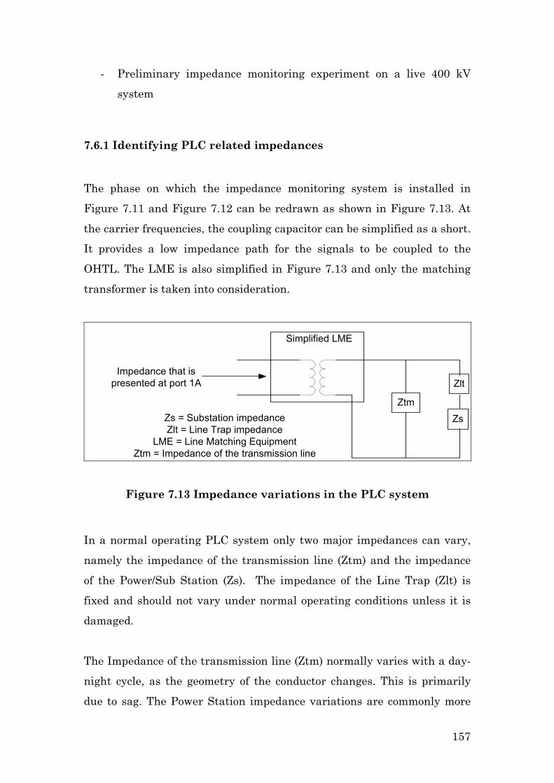
- Preliminary impedance monitoring experiment on a live 400 kV
system
7.6.1 Identifying PLC related impedances
The phase on which the impedance monitoring system is installed in
Figure 7.11 and Figure 7.12 can be redrawn as shown in Figure 7.13. At
the carrier frequencies, the coupling capacitor can be simplified as a short.
It provides a low impedance path for the signals to be coupled to the
OHTL. The LME is also simplified in Figure 7.13 and only the matching
transformer is taken into consideration.
ZtmZs
Zlt
Simplified LME
Impedance that ispresented at port 1A
Zs = Substation impedanceZlt = Line Trap impedance
LME = Line Matching EquipmentZtm = Impedance of the transmission line
Figure 7.13 Impedance variations in the PLC system
In a normal operating PLC system only two major impedances can vary,
namely the impedance of the transmission line (Ztm) and the impedance
of the Power/Sub Station (Zs). The impedance of the Line Trap (Zlt) is
fixed and should not vary under normal operating conditions unless it is
damaged.
The Impedance of the transmission line (Ztm) normally varies with a day-
night cycle, as the geometry of the conductor changes. This is primarily
due to sag. The Power Station impedance variations are commonly more
157
dramatic, as station equipment (such as transformers) is switched on and
off. Therefore it has a more step-like nature, but does not occur very often.
Variations in those impedances are transformed via the LME to be close to
75 ohm. Section 7.4 showed that the impedance monitoring technique is
most sensitive at 75 ohm and therefore the slightest changes in
transmission line impedance or power station impedance can be observed.
If the station impedance changes, the level of change will be known via the
PLC-IMP system and the level changes of the PLC-SAG tones can be
compensated for.
To obtain a more practical view of the proposed technique a sensitivity
analysis will be done, followed by a preliminary experiment on the live KA
OHTL.
7.6.2 PLC-IMP sensitivity analysis
The Koeberg-Acacia (KA) system will be used as basis for the following
discussion. For simplification of the analysis let us assume that all the
impedances are real.
The LME can be differently configured to match the impedance on the line
side to the characteristic impedance of the PLC system. The LME at
Acacia is strapped to match 390 Ω to 75 Ω . From this, the winding ratio of
the matching transformer can be easily computed as:
1
2
75390
nn
= 7.12
158

The impedance of the transmission line (Ztm) can be simulated for three
different heights at 250 kHz. The simulation default condition (as defined
in Chapter 3) was used to compute Ztm. Three simulations were done for
three different average heights (Table 7.2).
Table 7.2 OHTL Impedance of the KA OHTL
Average height [m] Absolute value of the OHTL impedance [ohm]
13 333.7
14 336
15 338
Let’s assume the Line trap impedance of 400 Ω at 250 kHz
Since the station impedance ( sZ ) is unknown, an analysis will be done
where sZ = (open circuit) and ∞ sZ = 0 (short circuit). With all the above
information we can redraw Figure 7.13 as Figure 7.14.
Ztm337.7
to338 Zs
Zlt400
sqrt(75/390)
Impedance that ispresented at port 1A
Zs = Substation impedanceZlt = Line Trap impedanceLMU = Line Matching Unit
Ztm = Impedance of the transmission line
Figure 7.14 Impedances at Acacia’s outer phase
Assume then 0sZ =
159

1_13
1_15
75 333.7 400 37.81 390 333.7 40075 338 400 37.6
390 338 400
port m
port m
Z
Z
⋅ = = + ⋅ = = +
Ω
Ω 7.13
Further assume then sZ = ∞
( )
( )
1_13
1_15
75 333,7 64.17 39075 338 65
390
port m
port m
Z
Z
= = Ω = = Ω
7.14
If these impedances were measured via the PLC-IMP monitoring system
the following results would be predicted by using the simulation done in
Figure 7.7.
For the scenario where 0sZ =
( )( )
1_13
1_15
14.09
14.01
h port m
h port m
F Z dB
F Z dB
=
= 7.15
For the scenario where sZ = ∞
( )( )
1_13
1_15
22.178
22.922
h port m
h port m
F Z dB
F Z dB
=
= 7.16
where is the transfer function of the isolation (Equation 7.10) as a
function of the impedance presented at Port 1 (
hF
1Z ).
The technique therefore provides a range of at least 8 dB to monitor the
station impedance ( sZ ) as described in this particular case. The sensitivity
160

would be further analysed via preliminary live line impedance experiment
on the KA system.
7.6.3 Preliminary impedance monitoring experiment
Due to the fact that no hardware change was needed for the PLC-IMP
system, the hybrid already installed at Acacia and used by the PLC-SAG
system could be utilised to perform the initial trial of the impedance
monitoring technique.
Referring to Figure 7.11, the local carrier tone (349.4 kHz) energised Port
2A of the measuring hybrid. The magnitude of the power at Port 3A of the
measurement hybrid was logged over a period of one week at a local
carrier frequency. The local carrier’s transmit level is very reliable and
constant under normal operating conditions. The results of the logged data
at Port 3A are shown in Figure 7.15.
A very clear day-night variation in the impedance can be noted. The
magnitude variation in the carrier signal level measured at Port 3A
(Figure 7.11) is in the order of 0.4 dB. This implies that the impedance
monitoring technique is sensitive enough to detect fractional variations of
ohms (Equation 7.15 and 7.16). The impedance variations of the station
can thus be monitored very accurately.
161

Figure 7.15 Measured variations in the magnitude of the insertion
loss over a period of one week on the KA OHTL
7.7 Conclusion
A step change in the logged data at Acacia Substation led to the reliability
of the PLC-SAG technique being questioned. This was alarming, since it
was unclear whether the problem could be overcome.
After a demanding period of time, a unique solution was found. By
exploring the complex isolation characteristics of the hybrid, it was found
that the hybrid could be employed to measure the PLC impedance. This
technique proved to have the required sensitivity to measure the changes
in impedance. In the event of unexpected impedance change the PLC-SAG
calibration can be adjusted. Details of the PLC-IMP monitoring technique
and the interaction with the PLC-SAG system have still to be researched.
The new technique also could be used for real-time condition monitoring of
PLC hardware.
162

References:
[1] Everitt, W. L, Communication Engineering, Second Edition, McGraw-
Hill, New York, 1937, page 318.
[2] JH Cloete, Personal communication, University of Stellenbosch,
September 2005.
[3] ] Brown Boveri (BBC) application sheet for A9BM, Carrier combiner
Unit used for Phase to Phase Coupling, BBC stock no. henf 105 169 R1,
edition 1981.
[4] Funk, H., Wandel & Goltermann Operation manual “LevelPRO
/LevelPRO NT Control and Evaluation Software for SPM/PSM – 37..139”,
Edition: 02/99.09 (V3.0), 1999, page 4.4.
163

Chapter 8
Conclusions and Recommendations
8.1 Conclusions
This thesis has proved experimentally, by two independent case studies,
that the PLC system can be utilised to measure the average conductor
height variation of an OHTL very accurately. The technique of “tracking”
the OHTL conductor height is called the PLC-SAG technique or system.
The procedure of installing the PLC-SAG system is streamlined with the
simulation program as discussed in Chapter 3. A simulation methodology
was defined together with a criterion to select the PLC-SAG monitoring
tones’ frequencies.
Two experimental PLC-SAG installations were successfully made on live
400 kV transmission systems without interrupting the power supply
(Chapter 4).
The PLC-SAG calibration process was discussed, which involves direct
height measurements (Chapter 5 and 6). Once the measurements had
been performed the PLC-SAG system could be calibrated.
A PLC-SAG calibration problem was discovered which threatened the
practicality of the PLC-SAG technique (Chapter 7).
An innovative solution was found to address this PLC-SAG calibration
problem. The new system, called PLC-IMP, tracks the impedance of the
PLC system by taking advantage of all the characteristics of the
measurement hybrid.
164
One of the exceptional advantages of the PLC-IMP solution in the
framework of this research is that it uses the same measurement hybrid
as the PLC-SAG system. A single system integrating the PLC-SAG and
the PLC-IMP can now be proposed and will be discussed in the following
section.
The reason why the impedance monitoring technique was given its own
entity, PLC-IMP, and not incorporated into the PLC-SAG entity, was that
there is a potential market for a PLC-IMP product alone. The PLC-IMP
system can be implemented as a condition monitoring system of the PLC
infrastructure. The PLC-SAG system cannot operate independently
without the PLC-IMP system.
The lifetime of an Ampacity system is in the order of 2-3 years, as the
power system is upgraded. Therefore the ability to quickly install a system
without major changes to the existing system is very important. In this
regard the PLC-SAG & PLC-IMP systems can be quickly installed and
calibrated, which makes this a highly competitive technique.
8.2 Recommendations
From the above study, measurable PLC-SAG tone level variations are
noted due to conductor sag and impedance changes in the system. Major
station impedance has a very low frequency of occurrence, which is
noticeably different to the day-to-day variations due to OHTL conductor
sag. In order to monitor the PLC-SAG tones efficiently it is very important
to distinguish between the two phenomena and to correctly compensate for
station impedance variations.
165

Development needs to be done on an integrated PLC-SAG & PLC-IMP
system. The following system is proposed as a starting point of this future
research.
At each monitoring station one PLC-SAG & PLC-IMP unit needs to be
installed. The PLC-SAG & PLC-IMP units comprise the following:
1) Generator 1: 75 ohm generator
2) Channel 1: High impedance voltage measurement in the time
domain
3) Channel 2: High impedance voltage measurement in the time
domain
The PLC-SAG & PLC-IMP units need to be connected to the existing PLC
system, as shown in Figure 8.1. The measurement hybrid does not
influence the PLC system significantly, as has been discussed in Chapter
4.
Table 8.1 Modes of operation for the PLC-SAG&PLC-IMP system
Mode PLC-SAG & PLC-IMP UNIT A PLC-SAG & PLC-IMP UNIT B
1) PLC-IMP at Station A GEN 1, CH 1 and CH 2 -
2) PLC-SAG A to B GEN 1 CH 2
3) PLC-IMP at Station B - GEN 1, CH 1 and CH 2
4) PLC-SAG B to A CH 2 GEN 1
166
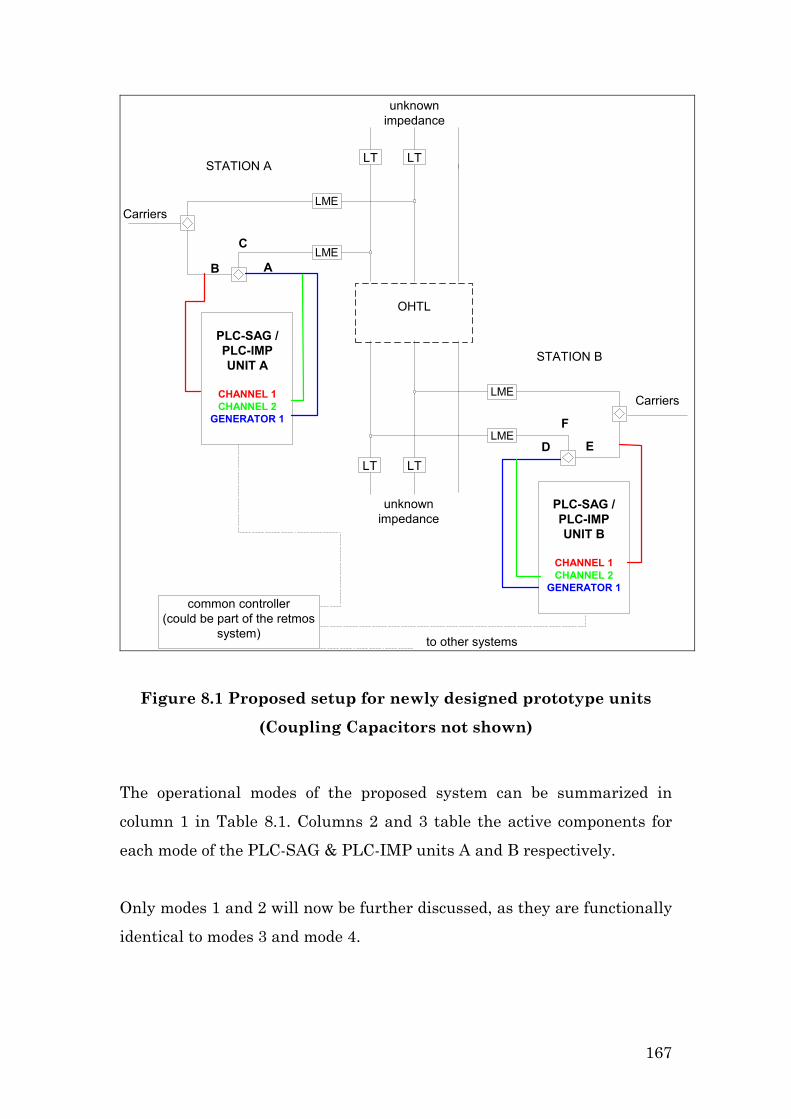
LME
LME
unknownimpedance
LT LT
LTLT
LME
LME
PLC-SAG /PLC-IMPUNIT A
CHANNEL 2GENERATOR 1
AB
C
common controller(could be part of the retmos
system)to other systems
unknownimpedance
STATION A
STATION B
D E
F
Carriers
Carriers
PLC-SAG /PLC-IMPUNIT B
CHANNEL 2GENERATOR 1
OHTL
CHANNEL 1
CHANNEL 1
Figure 8.1 Proposed setup for newly designed prototype units
(Coupling Capacitors not shown)
The operational modes of the proposed system can be summarized in
column 1 in Table 8.1. Columns 2 and 3 table the active components for
each mode of the PLC-SAG & PLC-IMP units A and B respectively.
Only modes 1 and 2 will now be further discussed, as they are functionally
identical to modes 3 and mode 4.
167

8.2.1 Mode 1: PLC-IMP at Station A
In this mode the PLC impedance at point C in Figure 8.1 is measured.
Significant impedance variations, which influence the PLC-SAG system,
can be tracked by using the monitoring hybrid as a sensitive impedance-
monitoring device (Chapter 7). By tracing the PLC impedance, the PLC-
SAG calibration values can be compensated for in the event of an
impedance change.
8.2.2 Mode 2: PLC-SAG A to B
In this mode the PLC-SAG tones are transmitted at station A and logged
at Station B. As proved in this thesis, by a straightforward action of
transmitting and receiving specially coupled tones, the average conductor
height can be tracked very accurately. Mode 2 and Mode 4 form part of the
duplex logging system as described in Chapter 4.
168
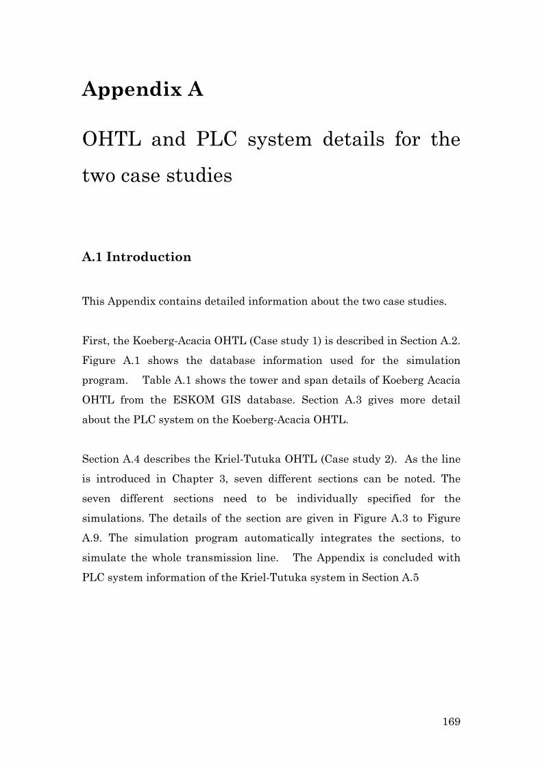
Appendix A
OHTL and PLC system details for the
two case studies
A.1 Introduction
This Appendix contains detailed information about the two case studies.
First, the Koeberg-Acacia OHTL (Case study 1) is described in Section A.2.
Figure A.1 shows the database information used for the simulation
program. Table A.1 shows the tower and span details of Koeberg Acacia
OHTL from the ESKOM GIS database. Section A.3 gives more detail
about the PLC system on the Koeberg-Acacia OHTL.
Section A.4 describes the Kriel-Tutuka OHTL (Case study 2). As the line
is introduced in Chapter 3, seven different sections can be noted. The
seven different sections need to be individually specified for the
simulations. The details of the section are given in Figure A.3 to Figure
A.9. The simulation program automatically integrates the sections, to
simulate the whole transmission line. The Appendix is concluded with
PLC system information of the Kriel-Tutuka system in Section A.5
169
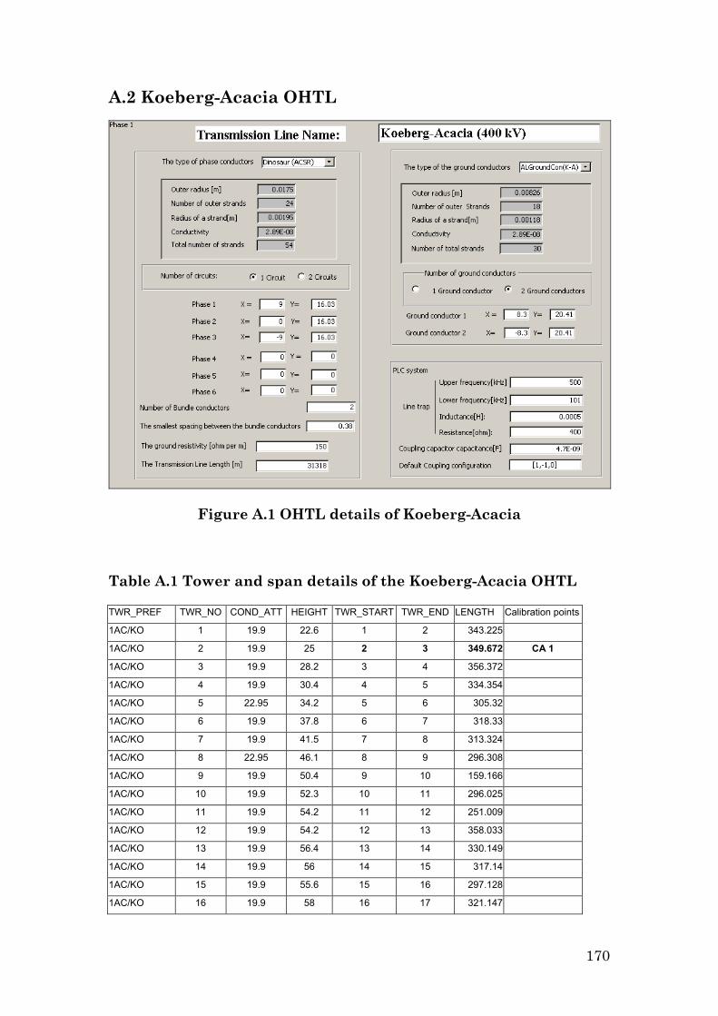
A.2 Koeberg-Acacia OHTL
Figure A.1 OHTL details of Koeberg-Acacia
Table A.1 Tower and span details of the Koeberg-Acacia OHTL
TWR_PREF TWR_NO COND_ATT HEIGHT TWR_START TWR_END LENGTH Calibration points
1AC/KO 1 19.9 22.6 1 2 343.225
1AC/KO 2 19.9 25 2 3 349.672 CA 1
1AC/KO 3 19.9 28.2 3 4 356.372
1AC/KO 4 19.9 30.4 4 5 334.354
1AC/KO 5 22.95 34.2 5 6 305.32
1AC/KO 6 19.9 37.8 6 7 318.33
1AC/KO 7 19.9 41.5 7 8 313.324
1AC/KO 8 22.95 46.1 8 9 296.308
1AC/KO 9 19.9 50.4 9 10 159.166
1AC/KO 10 19.9 52.3 10 11 296.025
1AC/KO 11 19.9 54.2 11 12 251.009
1AC/KO 12 19.9 54.2 12 13 358.033
1AC/KO 13 19.9 56.4 13 14 330.149
1AC/KO 14 19.9 56 14 15 317.14
1AC/KO 15 19.9 55.6 15 16 297.128
1AC/KO 16 19.9 58 16 17 321.147
170
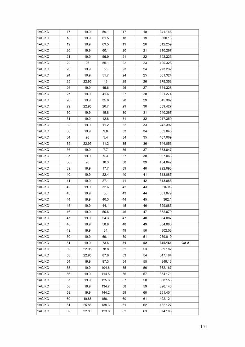
1AC/KO 17 19.9 59.1 17 18 341.148
1AC/KO 18 19.9 61.5 18 19 300.13
1AC/KO 19 19.9 63.5 19 20 312.259
1AC/KO 20 19.9 60.1 20 21 310.267
1AC/KO 21 19.9 56.9 21 22 392.325
1AC/KO 22 26 55.1 22 23 400.328
1AC/KO 23 19.9 55 23 24 273.232
1AC/KO 24 19.9 51.7 24 25 361.324
1AC/KO 25 22.95 49 25 26 379.353
1AC/KO 26 19.9 45.6 26 27 354.328
1AC/KO 27 19.9 41.6 27 28 301.274
1AC/KO 28 19.9 35.8 28 29 345.382
1AC/KO 29 22.95 26.7 29 30 389.427
1AC/KO 30 19.9 15.8 30 31 240.267
1AC/KO 31 19.9 12.8 31 32 217.359
1AC/KO 32 19.9 11.2 32 33 242.392
1AC/KO 33 19.9 9.8 33 34 302.045
1AC/KO 34 26 5.4 34 35 467.069
1AC/KO 35 22.95 11.2 35 36 344.053
1AC/KO 36 19.9 7.7 36 37 333.047
1AC/KO 37 19.9 9.3 37 38 397.063
1AC/KO 38 26 10.3 38 39 404.042
1AC/KO 39 19.9 17.7 39 40 292.093
1AC/KO 40 19.9 22.4 40 41 313.087
1AC/KO 41 19.9 27.1 41 42 313.086
1AC/KO 42 19.9 32.6 42 43 316.08
1AC/KO 43 19.9 36 43 44 301.079
1AC/KO 44 19.9 40.3 44 45 362.1
1AC/KO 45 19.9 44.1 45 46 329.085
1AC/KO 46 19.9 50.6 46 47 332.079
1AC/KO 47 19.9 54.3 47 48 334.087
1AC/KO 48 19.9 58.8 48 49 334.086
1AC/KO 49 19.9 64 49 50 302.03
1AC/KO 50 19.9 69.1 50 51 289.019
1AC/KO 51 19.9 73.6 51 52 345.161 CA 2
1AC/KO 52 22.95 78.8 52 53 369.182
1AC/KO 53 22.95 87.6 53 54 347.164
1AC/KO 54 19.9 97.3 54 55 349.16
1AC/KO 55 19.9 104.6 55 56 362.167
1AC/KO 56 19.9 114.5 56 57 354.171
1AC/KO 57 19.9 125.8 57 58 338.153
1AC/KO 58 19.9 134.7 58 59 326.146
1AC/KO 59 19.9 144.2 59 60 251.404
1AC/KO 60 19.86 150.1 60 61 422.121
1AC/KO 61 25.86 139.3 61 62 432.127
1AC/KO 62 22.86 123.8 62 63 374.106
171
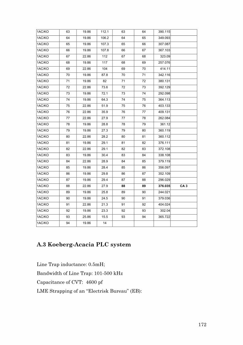
1AC/KO 63 19.86 112.1 63 64 390.115
1AC/KO 64 19.86 106.2 64 65 349.093
1AC/KO 65 19.86 107.3 65 66 307.087
1AC/KO 66 19.86 107.8 66 67 367.103
1AC/KO 67 22.86 112 67 68 323.09
1AC/KO 68 19.86 117 68 69 257.076
1AC/KO 69 22.86 104 69 70 414.11
1AC/KO 70 19.86 87.8 70 71 342.116
1AC/KO 71 19.86 82 71 72 380.131
1AC/KO 72 22.86 73.6 72 73 392.129
1AC/KO 73 19.86 72.1 73 74 292.098
1AC/KO 74 19.86 64.3 74 75 364.113
1AC/KO 75 22.86 51.9 75 76 403.133
1AC/KO 76 22.86 35.9 76 77 409.131
1AC/KO 77 22.86 27.9 77 78 262.084
1AC/KO 78 19.86 28.8 78 79 361.12
1AC/KO 79 19.86 27.3 79 80 360.119
1AC/KO 80 22.86 28.2 80 81 360.112
1AC/KO 81 19.86 29.1 81 82 376.111
1AC/KO 82 22.86 29.1 82 83 372.108
1AC/KO 83 19.86 30.4 83 84 338.108
1AC/KO 84 22.86 28.9 84 85 379.119
1AC/KO 85 19.86 28.4 85 86 356.097
1AC/KO 86 19.86 29.8 86 87 352.109
1AC/KO 87 19.86 29.4 87 88 296.029
1AC/KO 88 22.86 27.9 88 89 376.035 CA 3
1AC/KO 89 19.86 25.8 89 90 244.021
1AC/KO 90 19.86 24.5 90 91 379.036
1AC/KO 91 22.86 21.3 91 92 404.024
1AC/KO 92 19.86 23.3 92 93 302.04
1AC/KO 93 25.86 15.5 93 94 365.722
1AC/KO 94 19.86 14
A.3 Koeberg-Acacia PLC system
Line Trap inductance: 0.5mH;
Bandwidth of Line Trap: 101-500 kHz
Capacitance of CVT: 4600 pf
LME Strapping of an “Electrisk Bureau” (EB):
172
B3 A1B5 A3
A6A7
B2 A2B4 A7B12
From the 75 ohm cable
To the CVT
Figure A.2 LME strapping at Koeberg and Acacia for a standard
(“Electrisk Bureau” LME)
A.4 Kriel-Tutuka OHTL
Figure A.3 Section A of KT
173
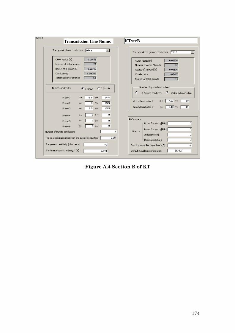
Figure A.4 Section B of KT
174

Figure A.5 Section C of KT
Figure A.6 Section D of KT
175

Figure A.7 Section E of KT
Figure A.8 Section F of KT
176

Figure A.9 Section G of KT
Table A.2 Tower and span details of the Kriel-Tutuka OHTL
TWR_PREF TWR_NO COND_ATT HEIGHT TWR_START TWR_END LENGTH Calibration points
-------- ---- --------- --------- ---- ---- ---------
1KR/TU 1 19.86 1621.5 1 2 213.84
1KR/TU 2 25.86 1616.7 2 3 225.819
1KR/TU 3 19.86 1613.8 3 4 202.842
1KR/TU 4 19.86 1610.6 4 5 412.04
1KR/TU 5 25.86 1619.1 5 6 358.029
1KR/TU 6 19.86 1616.8 6 7 346.023
1KR/TU 7 19.86 1614.7 7 8 335.036
1KR/TU 8 19.86 1612.5 8 9 326.027
1KR/TU 9 19.86 1612.1 9 10 342.005
1KR/TU 10 19.86 1609.6 10 11 311
1KR/TU 11 25.86 1601.9 11 12 481.012
1KR/TU 12 25.86 1604.1 12 13 222.001
1KR/TU 13 19.86 1617 13 14 196.928
1KR/TU 14 19.86 1616.5 14 15 412.617 CA 1
1KR/TU 15 25.86 1617.9 15 16 408.622
1KR/TU 16 22.5 1622.2 16 17 333.35
1KR/TU 17 25.5 1622 17 18 278.205
1KR/TU 18 24 1611.2 18 19 357.882
1KR/TU 19 27 1597 19 20 533.833
177

1KR/TU 20 27 1603.4 20 21 453.852
178
1KR/TU 64 33 1644.5 64 65 507.979
1KR/TU 65 30 1648.1 65 66 489.984
1KR/TU 21 27 1592.9 21 22 399.867
1KR/TU 22 25.5 1588 22 23 502.838
1KR/TU 23 25.5 1595.6 23 24 403.874
1KR/TU 24 24 1606.8 24 25 471.853
1KR/TU 25 28.5 1616.9 25 26 256.113
1KR/TU 26 27 1623.5 26 27 343.103
1KR/TU 27 22.5 1626.6 27 28 460.925
1KR/TU 28 31.5 1619.4 28 29 514.918
1KR/TU 29 30 1612.2 29 30 483.92
1KR/TU 30 28.5 1611.5 30 31 503.925
1KR/TU 31 31.5 1603.4 31 32 495.912
1KR/TU 32 30 1589 32 33 497.927
1KR/TU 33 25.5 1576.8 33 34 311.246
1KR/TU 34 22.5 1581.8 34 35 413.769
1KR/TU 35 27 1587.2 35 36 471.732
1KR/TU 36 27 1569.5 36 37 450.743
1KR/TU 37 25.5 1572.6 37 38 451.749
1KR/TU 38 25.5 1578.5 38 39 394.775
1KR/TU 39 21 1581 39 40 362.493
1KR/TU 40 19.5 1584.8 40 41 265.477
1KR/TU 41 25.5 1587.4 41 42 466.316
1KR/TU 42 33 1595.1 42 43 498.374
1KR/TU 43 25 1599.8 43 44 348.77
1KR/TU 44 18 1608 44 45 324.061
1KR/TU 45 22.5 1599.8 45 46 424.78
1KR/TU 46 27 1616.5 46 47 467.764
1KR/TU 47 27 1620.1 47 48 457.769
1KR/TU 48 25.5 1631.2 48 49 433.781
1KR/TU 49 27 1639.9 49 50 486.75
1KR/TU 50 28.5 1642.5 50 51 476.751
1KR/TU 51 28.5 1645.5 51 52 447.976
1KR/TU 52 22.5 1646.5 52 53 479.038
1KR/TU 53 31.5 1660.7 53 54 483.04
1KR/TU 54 30 1659.3 54 55 515.037
1KR/TU 55 31.5 1664 55 56 485.046
1KR/TU 56 28.5 1665 56 57 446.431
1KR/TU 57 27.5 1680.1 57 58 370.119
1KR/TU 58 28.5 1664.5 58 59 535.158
1KR/TU 59 27 1658.5 59 60 496.254
1KR/TU 60 30.5 1663.4 60 61 441.988
1KR/TU 61 33 1655.4 61 62 510.981
1KR/TU 62 24 1648 62 63 488.977
1KR/TU 63 43 1638.3 63 64 408.987

1KR/TU 66 31.5 1647 66 67 486.984
179
1KR/TU 110 28.5 1613.2 110 111 402.682
1KR/TU 111 25 1617.7 111 112 439.126
1KR/TU 67 28.5 1629.5 67 68 497.98
1KR/TU 68 31.5 1624.4 68 69 477.98
1KR/TU 69 30 1615.5 69 70 470.992
1KR/TU 70 28.5 1594.5 70 71 398.181
1KR/TU 71 22.5 1598.3 71 72 442.746
1KR/TU 72 28.5 1606.6 72 73 461.733
1KR/TU 73 29.5 1611.5 73 74 301.119
1KR/TU 74 22.5 1616 74 75 253.686
1KR/TU 75 18 1620 75 76 279.254
1KR/TU 76 19.5 1621.2 76 77 399.916
1KR/TU 77 25.5 1612.7 77 78 491.89
1KR/TU 78 31.5 1606.4 78 79 509.887
1KR/TU 79 31.5 1606.8 79 80 466.899
1KR/TU 80 30 1607 80 81 530.883
1KR/TU 81 28.5 1589 81 82 394.213
1KR/TU 82 22.5 1583.7 82 83 234.86
1KR/TU 83 18 1575.7 83 84 322.8
1KR/TU 84 28.5 1569 84 85 402.55
1KR/TU 85 19 1567.5 85 86 262.903
1KR/TU 86 19.86 1566.1 86 87 373.862
1KR/TU 87 19.86 1565.8 87 88 327.929
1KR/TU 88 11.8 0 88 89 69.347
1KR/TU 89 11.8 0 89 90 82.109
1KR/TU 90 11.8 0 90 91 90.252
1KR/TU 91 11.8 0 91 92 30.583
1KR/TU 92 8.8 0 92 93 44.078
1KR/TU 93 11.8 0 93 94 362.326
1KR/TU 94 27 1575 94 95 449.32
1KR/TU 95 28.5 1575.9 95 96 477.6
1KR/TU 96 31.5 1577.9 96 97 519.236
1KR/TU 97 28 1581.9 97 98 232.659
1KR/TU 98 33.5 1582.7 98 99 550.256
1KR/TU 99 47 1591.3 99 100 550.813
1KR/TU 100 22 1597.6 100 101 466.263
1KR/TU 101 31.5 1604.1 101 102 533.253
1KR/TU 102 31.5 1604.1 102 103 450.943
1KR/TU 103 22 1600.7 103 104 425.477
1KR/TU 104 22 1607.5 104 105 334.082
1KR/TU 105 19.5 1601.9 105 106 455.192
1KR/TU 106 27 1586.5 106 107 473.202
1KR/TU 107 27 1587.1 107 108 416.932
1KR/TU 108 24 1593.2 108 109 474.942
1KR/TU 109 27 1600.9 109 110 434.002
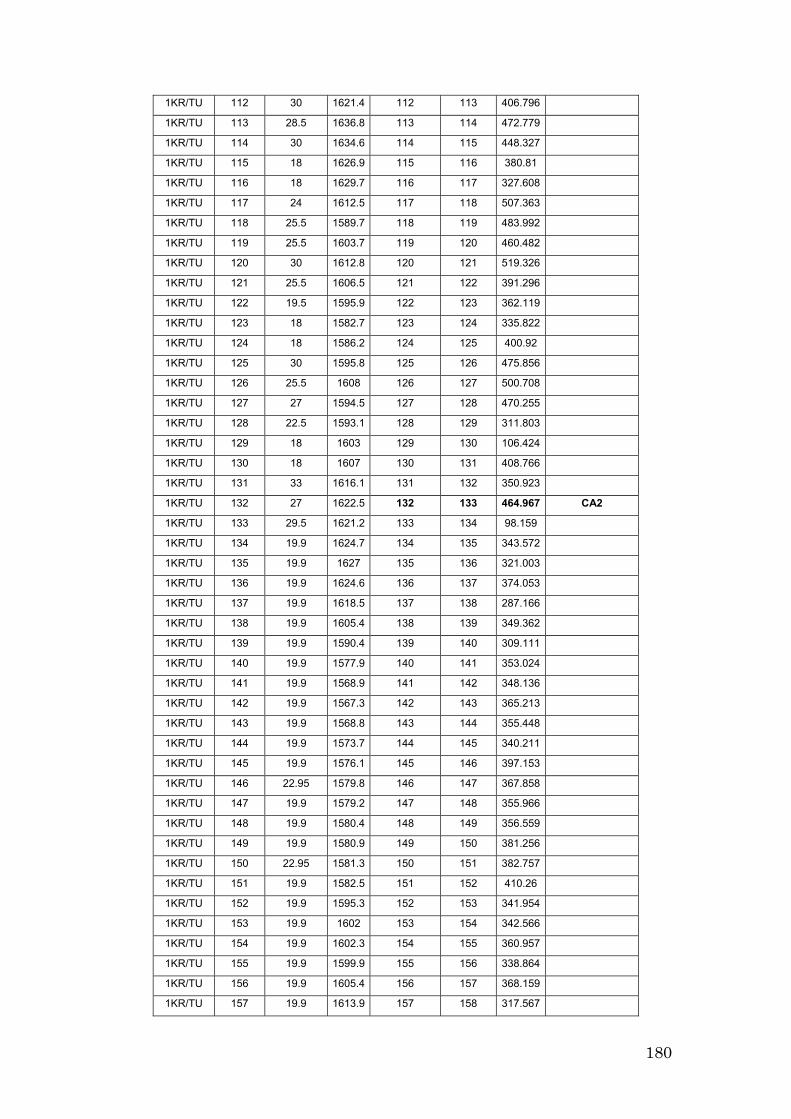
1KR/TU 112 30 1621.4 112 113 406.796
180
1KR/TU 156 19.9 1605.4 156 157 368.159
1KR/TU 157 19.9 1613.9 157 158 317.567
1KR/TU 113 28.5 1636.8 113 114 472.779
1KR/TU 114 30 1634.6 114 115 448.327
1KR/TU 115 18 1626.9 115 116 380.81
1KR/TU 116 18 1629.7 116 117 327.608
1KR/TU 117 24 1612.5 117 118 507.363
1KR/TU 118 25.5 1589.7 118 119 483.992
1KR/TU 119 25.5 1603.7 119 120 460.482
1KR/TU 120 30 1612.8 120 121 519.326
1KR/TU 121 25.5 1606.5 121 122 391.296
1KR/TU 122 19.5 1595.9 122 123 362.119
1KR/TU 123 18 1582.7 123 124 335.822
1KR/TU 124 18 1586.2 124 125 400.92
1KR/TU 125 30 1595.8 125 126 475.856
1KR/TU 126 25.5 1608 126 127 500.708
1KR/TU 127 27 1594.5 127 128 470.255
1KR/TU 128 22.5 1593.1 128 129 311.803
1KR/TU 129 18 1603 129 130 106.424
1KR/TU 130 18 1607 130 131 408.766
1KR/TU 131 33 1616.1 131 132 350.923
1KR/TU 132 27 1622.5 132 133 464.967 CA2
1KR/TU 133 29.5 1621.2 133 134 98.159
1KR/TU 134 19.9 1624.7 134 135 343.572
1KR/TU 135 19.9 1627 135 136 321.003
1KR/TU 136 19.9 1624.6 136 137 374.053
1KR/TU 137 19.9 1618.5 137 138 287.166
1KR/TU 138 19.9 1605.4 138 139 349.362
1KR/TU 139 19.9 1590.4 139 140 309.111
1KR/TU 140 19.9 1577.9 140 141 353.024
1KR/TU 141 19.9 1568.9 141 142 348.136
1KR/TU 142 19.9 1567.3 142 143 365.213
1KR/TU 143 19.9 1568.8 143 144 355.448
1KR/TU 144 19.9 1573.7 144 145 340.211
1KR/TU 145 19.9 1576.1 145 146 397.153
1KR/TU 146 22.95 1579.8 146 147 367.858
1KR/TU 147 19.9 1579.2 147 148 355.966
1KR/TU 148 19.9 1580.4 148 149 356.559
1KR/TU 149 19.9 1580.9 149 150 381.256
1KR/TU 150 22.95 1581.3 150 151 382.757
1KR/TU 151 19.9 1582.5 151 152 410.26
1KR/TU 152 19.9 1595.3 152 153 341.954
1KR/TU 153 19.9 1602 153 154 342.566
1KR/TU 154 19.9 1602.3 154 155 360.957
1KR/TU 155 19.9 1599.9 155 156 338.864
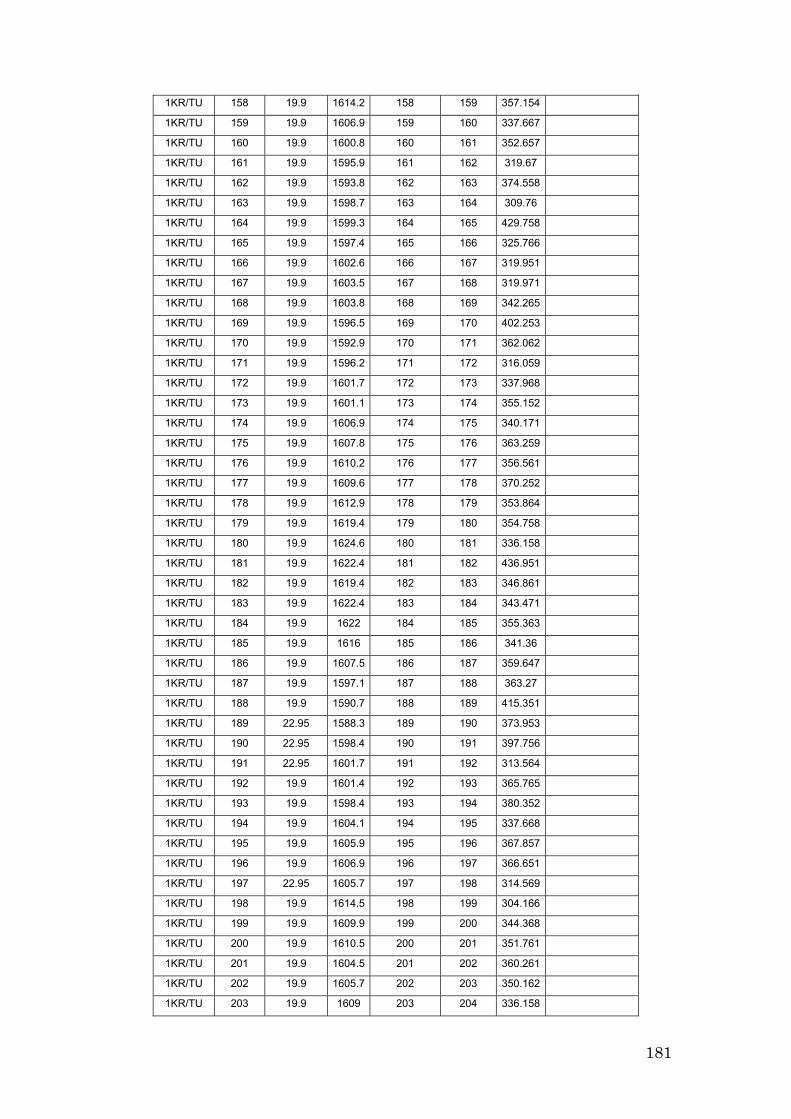
1KR/TU 158 19.9 1614.2 158 159 357.154
1KR/TU 159 19.9 1606.9 159 160 337.667
1KR/TU 160 19.9 1600.8 160 161 352.657
1KR/TU 161 19.9 1595.9 161 162 319.67
1KR/TU 162 19.9 1593.8 162 163 374.558
1KR/TU 163 19.9 1598.7 163 164 309.76
1KR/TU 164 19.9 1599.3 164 165 429.758
1KR/TU 165 19.9 1597.4 165 166 325.766
1KR/TU 166 19.9 1602.6 166 167 319.951
1KR/TU 167 19.9 1603.5 167 168 319.971
1KR/TU 168 19.9 1603.8 168 169 342.265
1KR/TU 169 19.9 1596.5 169 170 402.253
1KR/TU 170 19.9 1592.9 170 171 362.062
1KR/TU 171 19.9 1596.2 171 172 316.059
1KR/TU 172 19.9 1601.7 172 173 337.968
1KR/TU 173 19.9 1601.1 173 174 355.152
1KR/TU 174 19.9 1606.9 174 175 340.171
1KR/TU 175 19.9 1607.8 175 176 363.259
1KR/TU 176 1610.2 176 177 19.9 356.561
178 370.252
1KR/TU 178 19.9 1612.9 178 179 353.864
1KR/TU 179 19.9 1619.4 179 180 354.758
1KR/TU 180 19.9 1624.6 180 181 336.158
1KR/TU 181 19.9 1622.4 181 182 436.951
1KR/TU 182 19.9 1619.4 182 183 346.861
1KR/TU 183 19.9 1622.4 183 184 343.471
1KR/TU 184 19.9 1622 184 185 355.363
1KR/TU 185 19.9 1616 185 186 341.36
1KR/TU 186 19.9 1607.5 186 187 359.647
1KR/TU 187 19.9 1597.1 187 188 363.27
1KR/TU 188 19.9 1590.7 188 189 415.351
1KR/TU 189 22.95 1588.3 189 190 373.953
1KR/TU 190 22.95 1598.4 190 191 397.756
1KR/TU 191 22.95 1601.7 191 192 313.564
1KR/TU 192 19.9 1601.4 192 193 365.765
1KR/TU 193 19.9 1598.4 193 194 380.352
1KR/TU 194 19.9 1604.1 194 195 337.668
1KR/TU 195 19.9 1605.9 195 196 367.857
1KR/TU 196 19.9 1606.9 196 197 366.651
1KR/TU 197 22.95 1605.7 197 198 314.569
1KR/TU 198 19.9 1614.5 198 199 304.166
1KR/TU 199 19.9 1609.9 199 200 344.368
1KR/TU 200 19.9 1610.5 200 201 351.761
1KR/TU 201 19.9 1604.5 201 202 360.261
1KR/TU 202 19.9 1605.7 202 203 350.162
1KR/TU 203 19.9 1609 203 204 336.158
1KR/TU 177 19.9 1609.6 177
181
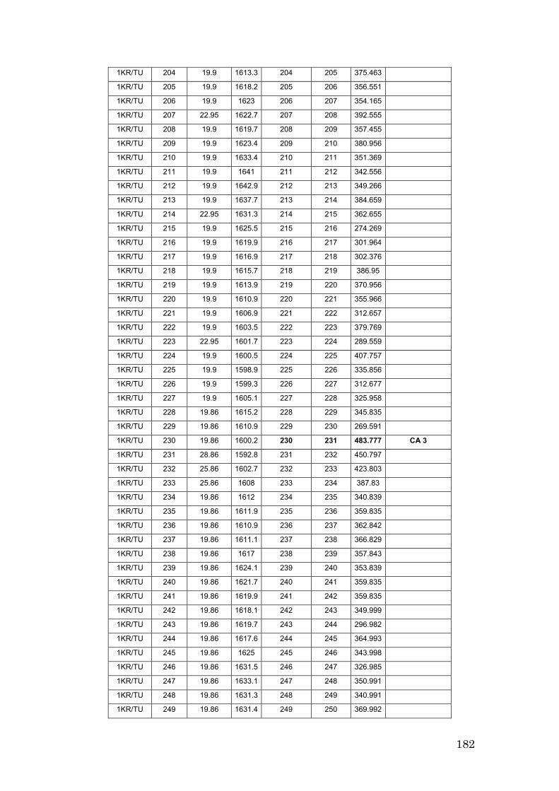
1KR/TU 204 19.9 1613.3 204 205 375.463
1KR/TU 205 19.9 1618.2 205 206 356.551
1KR/TU 206 19.9 1623 206 207 354.165
1KR/TU 207 22.95 1622.7 207 208 392.555
1KR/TU 208 19.9 1619.7 208 209 357.455
1KR/TU 209 19.9 1623.4 209 210 380.956
1KR/TU 210 19.9 1633.4 210 211 351.369
1KR/TU 211 19.9 1641 211 212 342.556
1KR/TU 212 19.9 1642.9 212 213 349.266
1KR/TU 213 19.9 1637.7 213 214 384.659
1KR/TU 214 22.95 1631.3 214 215 362.655
1KR/TU 215 19.9 1625.5 215 216 274.269
1KR/TU 216 19.9 1619.9 216 217 301.964
1KR/TU 217 19.9 1616.9 217 218 302.376
1KR/TU 218 19.9 1615.7 218 219 386.95
1KR/TU 219 19.9 1613.9 219 220 370.956
1KR/TU 220 19.9 1610.9 220 221 355.966
1KR/TU 221 19.9 1606.9 221 222 312.657
1KR/TU 222 19.9 1603.5 222 223 379.769
1KR/TU 223 22.95 1601.7 223 224 289.559
1KR/TU 224 19.9 1600.5 224 225 407.757
1KR/TU 225 19.9 1598.9 225 226 335.856
1KR/TU 226 19.9 1599.3 226 227 312.677
1KR/TU 227 19.9 1605.1 227 228 325.958
1KR/TU 228 19.86 1615.2 228 229 345.835
1KR/TU 229 19.86 1610.9 229 230 269.591
1KR/TU 230 19.86 1600.2 230 231 483.777 CA 3
1KR/TU 231 28.86 1592.8 231 232 450.797
1KR/TU 232 25.86 1602.7 232 233 423.803
1KR/TU 233 25.86 1608 233 234 387.83
1KR/TU 234 19.86 1612 234 235 340.839
1KR/TU 235 19.86 1611.9 235 236 359.835
1KR/TU 236 19.86 1610.9 236 237 362.842
1KR/TU 237 19.86 1611.1 237 238 366.829
1KR/TU 238 19.86 1617 238 239 357.843
1KR/TU 239 19.86 1624.1 239 240 353.839
1KR/TU 240 19.86 1621.7 240 241 359.835
1KR/TU 241 19.86 1619.9 241 242 359.835
1KR/TU 242 19.86 1618.1 242 243 349.999
1KR/TU 243 19.86 1619.7 243 244 296.982
1KR/TU 244 19.86 1617.6 244 245 364.993
1KR/TU 245 19.86 1625 245 246 343.998
1KR/TU 246 19.86 1631.5 246 247 326.985
1KR/TU 247 19.86 1633.1 247 248 350.991
1KR/TU 248 19.86 1631.3 248 249 340.991
1KR/TU 249 19.86 1631.4 249 250 369.992
182

1KR/TU 250 28.86 1641.3 250 251 476.993
1KR/TU 251 31.86 1631.4 251 252 470.985
1KR/TU 252 19.86 1619.7 252 253 348.985
1KR/TU 253 19.86 1626.1 253 254 353.998
1KR/TU 254 19.86 1633 254 255 268.983
1KR/TU 255 19.86 1628.5 255 256 375.541
1KR/TU 256 19.86 1617.5 256 257 368.519
1KR/TU 257 19.86 1608.9 257 258 433.775
1KR/TU 258 19.86 1611 258 259 332.357
1KR/TU 259 19.86 1612.7 259 260 384.575
1KR/TU 260 19.86 1608.3 260 261 411.682
1KR/TU 261 19.86 1606.7 261 262 318.303
1KR/TU 262 19.86 1614.7 262 263 335.375
1KR/TU 263 19.86 1619 263 264 324.333
1KR/TU 264 19.86 1611.8 264 265 331.355
1KR/TU 265 19.86 1619.5
A.5 Kriel-Tutuka PLC System
LME Strapping of an “Electrisk Bureau” (EB):
Line Trap inductance: 0.5mH;
Bandwidth of Line Trap at Kriel: 104-500 kHz
Bandwidth of Line Trap at Tutuka: 101-500 kHz
Capacitance of CVT at Kriel: 4700 pF
Capacitance of CVT at Tutuka: 7000 pF
0.93mH Zo = 230Zo = 75 21mH
Drain coil
F(A2)F(A7)F(B4)F(B2)T(A4)
T(A3) T(A1) T(A7)
20 nF 20 nF
Figure A.10 LME strapping at Kriel and Tutuka
183

Appendix B
Additional information about Koeberg-
Acacia and Kriel-Tutuka operational
PLCs
B.1 Introduction
This Appendix primarily gives more information about the neighbouring
systems in the PLC frequency range (50-500 kHz). This information is
needed in order to allocate the frequencies for the PLC-SAG monitoring
tones.
Acacia-Koeberg (Case study 1):
Section B.2 contains a table with all the neighbouring carrier frequencies.
Section B.3 shows a map with aviation beacon frequencies. An enlarged
version of the frequency scan is given in Section B.4 and shown in Figure
B.2. The neighbouring carriers (letter as specified in Table B.1) and the
aviation frequencies (short black lines) are indicated on this frequency
scan. The measurement bandwidth of the frequency scan was 20 Hz and
the sweep rate = 22 hours. The scan was done with a HP 3586A selective
level meter, which was controlled by a desktop computer.
184

Kriel-Tutuka (Case study 2):
Section B.5 contains a table with the neighbouring PLC system
frequencies for the Kriel-Tutuka PLC link. The table contains information
of neighbouring carriers: 1 busbar away (black) from Kriel and Tutuka PS;
2 busbars away (grey) and 3 busbars away (light grey). The rows between
Kriel and Tutuka Power Station are filled with light grey, for reference
purposes. The columns that are filled from top to bottom in grey indicate
frequencies, which are occupied by an open wire Telkom carrier systems.
These frequencies are avoided to prevent interference with the Telkom
carrier circuits. The red indicates an overlapping scenario were two same
frequency band is occupied by two different systems.
In Section B.6, the results of the KT frequency scan is shown. The scan
was preformed with a HP 3586 A selective voltmeter. The narrowest
bandwidth, 20 Hz, was used and the sweep time was approximately 22
hours which is similar to case study 1. Due to their great number, it was
not possible to identify all the carriers on the graph, as was done in the
previous case. There was no aviation beacon information in this area.
Studying Figure B.3, it may seem that some of the frequencies are
overlapping. Zoomed in figures are also given to show the frequency
separation between the PLC-SAG tones and the neighbouring systems. .
Mr Piet Lubbe, Eskom Transmission, gathered and processed all the
information required to create the two frequency tables in Section B.2 and
in Section B.4.
185
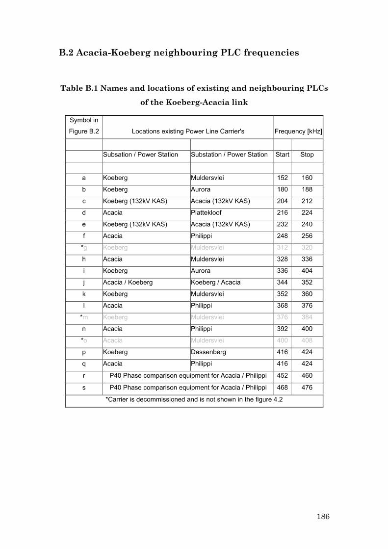
B.2 Acacia-Koeberg neighbouring PLC frequencies
Table B.1 Names and locations of existing and neighbouring PLCs
of the Koeberg-Acacia link
Symbol in
Figure B.2 Locations existing Power Line Carrier's Frequency [kHz]
Subsation / Power Station Substation / Power Station Start Stop
a Koeberg Muldersvlei 152 160
b Koeberg Aurora 180 188
c Koeberg (132kV KAS) Acacia (132kV KAS) 204 212
d Acacia Plattekloof 216 224
e Koeberg (132kV KAS) Acacia (132kV KAS) 232 240
f Acacia Philippi 248 256
*g Koeberg Muldersvlei 312 320
h Acacia Muldersvlei 328 336
i Koeberg Aurora 336 404
j Acacia / Koeberg Koeberg / Acacia 344 352
k Koeberg Muldersvlei 352 360
l Acacia Philippi 368 376
*m Koeberg Muldersvlei 376 384
n Acacia Philippi 392 400
*o Acacia Muldersvlei 400 408
p Koeberg Dassenberg 416 424
q Acacia Philippi 416 424
r P40 Phase comparison equipment for Acacia / Philippi 452 460
s P40 Phase comparison equipment for Acacia / Philippi 468 476
*Carrier is decommissioned and is not shown in the figure 4.2
186

B.3 Navigational Radio Beacon Frequencies (053/1839)
Figure B.1 Part (Western Cape) of the Navigational Radio Beacon
Frequencies map in South Africa (053/1839)
187

B.4 Koeberg-Acacia frequency scan
Figure B.2 100-520 kHz wideband measurement at Acacia Sub Station (2004/03/18-2004/03/19). See Table B.1 and
Figure B.1 for symbol definition.
188

B.5 Kriel-Tutuka neighbouring PLC frequencies (See paragraph B.1 for colour definitions)
189
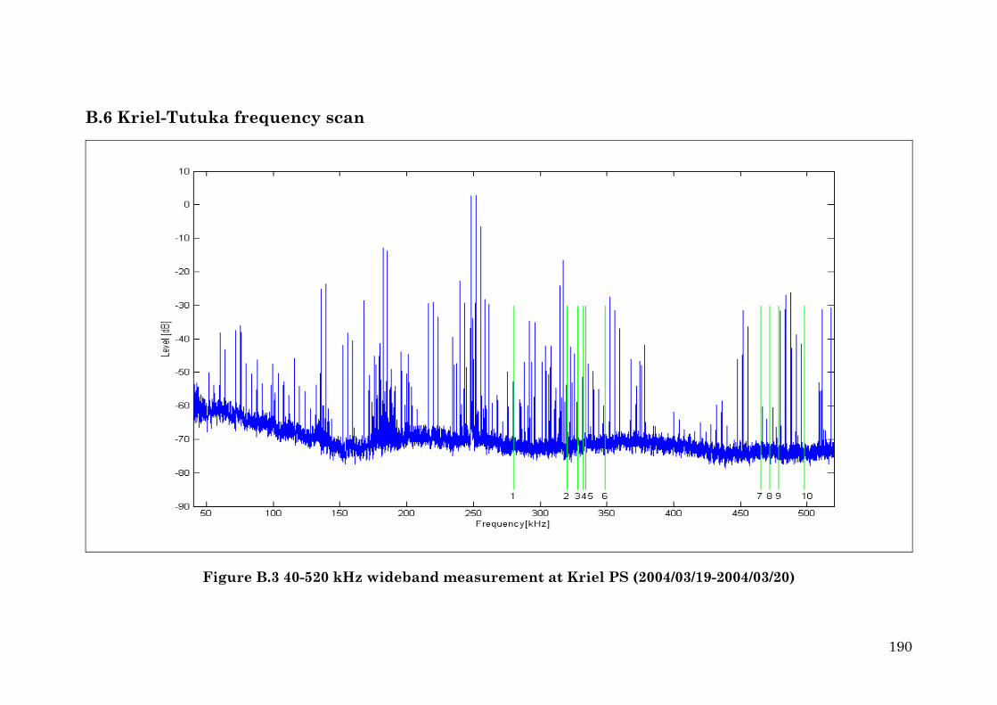
B.6 Kriel-Tutuka frequency scan
Figure B.3 40-520 kHz wideband measurement at Kriel PS (2004/03/19-2004/03/20)
190
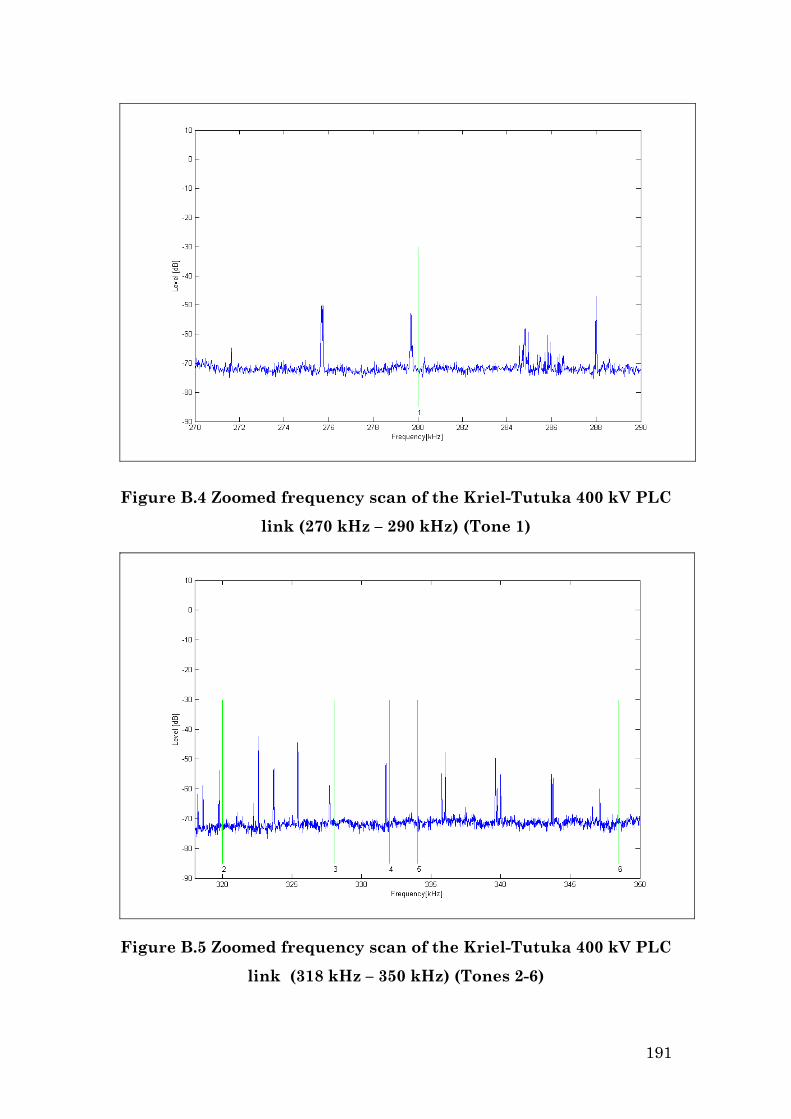
Figure B.4 Zoomed frequency scan of the Kriel-Tutuka 400 kV PLC
link (270 kHz – 290 kHz) (Tone 1)
Figure B.5 Zoomed frequency scan of the Kriel-Tutuka 400 kV PLC
link (318 kHz – 350 kHz) (Tones 2-6)
191
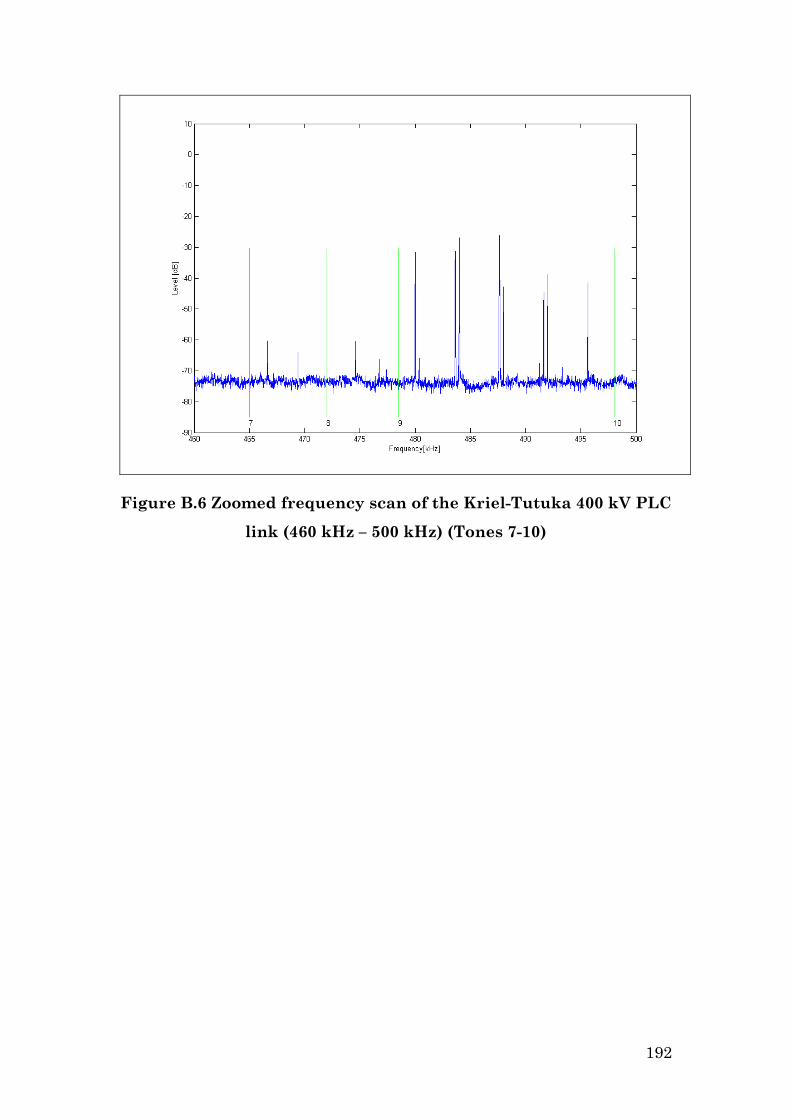
Figure B.6 Zoomed frequency scan of the Kriel-Tutuka 400 kV PLC
link (460 kHz – 500 kHz) (Tones 7-10)
192

Appendix C
Additional information about the
experimental transmitter and receiver
installations
C.1 Introduction
More information is given on the Transorb (Section C.2) and the amplifier
(Section C.3) used in the PLC-SAG hardware installations.
The design of the attenuator, which also has an impedance matching
function, is given in Section C.4.
The normal setting of receivers will be given in Section C.5.
C.2 Transorb datasheet
Photograph C.1 Transorb from Clear Line (Model 12-00109)
193

Table C.1 Data sheet of the Transorb (Model 12-00109)
Max. operating voltage +/- 5V dc +/- 24V dc +/- 5V dc
Max. operating current 0.3A 0.3A 0.3A
Max. discharge current ismax differential mode (8/20)
10kA 10kA 10kA
Max. discharge current
ismax common mode
(8/20)
10kA 10kA 10kA
Residual voltage
differential mode at 5kA
(8/20)
Approx. 40V Approx. 40V Approx. 40V
Residual voltage common
mode at 5kA (8/20) Approx. 120V Approx. 120V Approx. 120V
Insertion loss at 10MHz 0.08 dB 0.08 dB 0.08 dB
Connectors BNC BNC N-type
Temperature range -10°C to + 70°C -10°C to + 70°C -10°C to + 70°C
Application Cheapernet 10 Base 2 Arcnet, CCTV Ethernet 10 Base 5
Order Code 12-00109 12-00112 12-00049
C.3 Amplifier
Photograph C.2 Amplifier from Mini-Circuits (model ZHL-32A)
194

Table C.2 Data sheet of the Amplifier (model ZHL-32A)
Gain (dB) Directivity (dB) VSWR FREQ
(MHz) 23V 24V 24.5V 23V 24V 24.5V IN OUT
N.F.
(dB)
Pout(dBm)
(@1dB COMPR)
0.05 26.65 26.67 26.69 15.1 15.1 15.1 1.02 2.00 - 32.21
0.14 27.27 27.30 27.31 13.8 13.8 13.8 1.03 1.65 - 32.68
0.68 27.41 27.44 27.45 13.5 13.5 13.4 1.04 1.58 - 32.83
3.2 27.57 27.60 27.63 13.1 13.1 13.2 1.08 1.62 - 32.99
15.3 27.45 27.48 27.49 13.3 13.2 13.2 1.20 1.61 5.85 32.76
46.7 27.12 27.16 27.18 13.5 13.5 13.4 1.38 1.52 6.00 31.88
56.7 27.18 27.21 27.24 13.4 13.5 13.4 1.39 1.56 6.04 31.83
66.7 27.35 27.38 27.40 13.2 13.3 13.3 1.36 1.56 6.04 31.43
73.4 27.55 27.59 27.60 13.0 13.1 13.1 1.33 1.57 6.02 31.30
80.0 27.76 27.81 27.83 13.0 13.0 12.9 1.30 1.56 5.99 31.33
90.0 28.00 28.04 28.06 12.9 12.7 12.8 1.28 1.50 6.00 30.98
100.0 28.03 12.9 13.0 1.39
27.75 27.83 13.1 13.2 1.29 30.06
27.37 13.6 13.5 1.36 6.31
26.64 26.72 14.2 14.2 14.2 1.15 29.82
27.97 28.05 12.9 1.29 6.08 30.47
110.0 27.80 13.2 1.32 6.19
120.0 27.32 27.40 13.6 1.19 30.17
130.0 26.71 1.43 6.45
C.4 Impedance matching network and attenuator
The specifications for the design are the following:
c) 10 dB attenuation.
Figure C.1 demonstrates these design criteria.
a) Input impedance of port 1 must be 50 ohm (to match the spectrum
analyser with the system)
b) Input impedance of port 2 must be 75 ohm (to terminate the
additional symmetrical hybrid correctly)
195

Figure C.1 Impedance matching network (and 10 dB attenuator)
illustrating the design criteria.
Figure C.2 shows the proposed circuit layout with x, y and z as the
unknown resistors.
Port 150 ohms
Y Z
X Port 275 ohms
Figure C.2 Circuit layout of the impedance matching circuit
From the first two design criteria the following equation can be derived.
(75 )5075
z x yz x
+ = + + +
(50 )7550
y x zy x
+= + + +
Assuming port 2 is connected to a matched (75 ohm) source, which
produces 1V rms over the terminals of port 2. Then the power delivered by
the 1 V supply at port 2 is
196
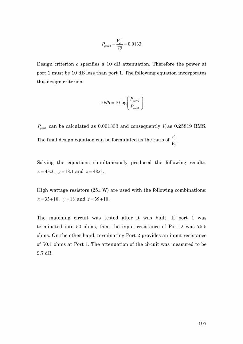
22
2 0.013375portVP = =
Design criterion c specifies a 10 dB attenuation. Therefore the power at
port 1 must be 10 dB less than port 1. The following equation incorporates
this design criterion
2
1
10 10log port
port
PdB
P
=
1portP can be calculated as 0.001333 and consequently V as 0.25819 RMS.
The final design equation can be formulated as the ratio of
1
1
2
VV
.
High wattage resistors (25± W) are used with the following combinations:
, and .
Solving the equations simultaneously produced the following results:
, and . 43.3x = 18.1y = 48.6z =
33 10x = + 18y = 39 10z = +
The matching circuit was tested after it was built. If port 1 was
terminated into 50 ohms, then the input resistance of Port 2 was 75.5
ohms. On the other hand, terminating Port 2 provides an input resistance
of 50.1 ohms at Port 1. The attenuation of the circuit was measured to be
9.7 dB.
197

C.5 Receiver settings for PLC-SAG tone monitoring
HP 3586A at Acacia Sub Station
• 50 ohm impedance (the attenuator also match the 50 ohm to
the 75 ohm characteristic impedance)
• 20 Hz selective filter
• Unit setting dBm
• 75 ohm - high impedance setting
• Average on
PSM 37 Wandel & Goltermann at Kriel Power Station
• 25 Hz selective filter
• Unit setting dBm
• Average on
HP 3586A at Kriel Power Station
• 20 Hz selective filter
• Unit setting dBm
• 75 ohm – high impedance setting
• Average on
• Battery standby function: off
198

Appendix D
PLC tone during the outage on the KT
OHTL dated 2004/05/04
D.1 Introduction
Appendix D describes how the signals were amended to compensate for
the outage on 2004/05/04. The black graph in the following figures
represents the compensated attenuation. The red dots highlight the signal
level just before and after the line was switched off and on. The blue graph
shows the actual recorded signal level.
Adding a constant value of attenuation to the signal in the region of the
outage made the compensation. The exact level in each case is given in the
titles of the relevant figure.
199

D.2 The 5 relevant tones
06:00 07:00 08:00 09:00 10:00 11:00 12:00 13:00 14:00 15:00 16:00 17:00 18:00-42
-41.5
-41
-40.5
-40
-39.5
-39
-38.5
-38
-37.5
Time
Leve
l [dB
m]
Figure D.1 Tone 3 - 2.653 dB added during the period of the outage
06:00 07:00 08:00 09:00 10:00 11:00 12:00 13:00 14:00 15:00 16:00 17:00 18:00-42.5
-42
-41.5
-41
-40.5
-40
-39.5
-39
-38.5
Time
Leve
l [dB
m]
Figure D.2 Tone 4 - 2.671 dB added during the period of the outage
200

06:00 07:00 08:00 09:00 10:00 11:00 12:00 13:00 14:00 15:00 16:00 17:00 18:00-43.5
-43
-42.5
-42
-41.5
-41
-40.5
-40
-39.5
-39
Time
Leve
l [dB
m]
Figure D.3 Tone 5 - 2.975 dB added during the period of the outage
06:00 07:00 08:00 09:00 10:00 11:00 12:00 13:00 14:00 15:00 16:00 17:00 18:00-44.5
-44
-43.5
-43
-42.5
-42
-41.5
-41
Time
Leve
l [dB
m]
Figure D.4 Tone 6 - 2.031 dB added during the period of the outage
201
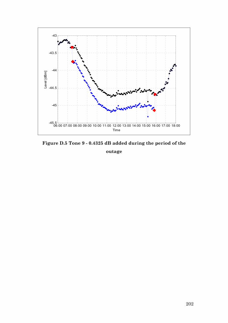
06:00 07:00 08:00 09:00 10:00 11:00 12:00 13:00 14:00 15:00 16:00 17:00 18:00-45.5
-45
-44.5
-44
-43.5
-43
Time
Leve
l [dB
m]
Figure D.5 Tone 9 - 0.4325 dB added during the period of the
outage
202