Embed Size (px)
Citation preview


APPROVAL SHEET
Title of Thesis: REAL-TIME GPU SURFACE CURVATURE ESTIMATION
Name of Candidate: Wesley GriffinMaster of Science, 2010
Thesis and Abstract Approved:Dr. Marc OlanoAssociate ProfessorDepartment of Computer Science andElectrical Engineering
Date Approved:

CURRICULUM VITAE
Wesley Griffin
9835 Rainleaf Ct.
Columbia, MD 21046
Education
May 2010 M.S. in Computer Science, University of Maryland, Baltimore County
May 2007 B.S. summa cum laude in Computer Science, University of Maryland
University College
Publications
K. Das, K. Bhaduri, S. Arora, W. Griffin, K. Borne, C. Giannella, H. Kargupta. “Scal-
able Distributed Change Detection from Astronomy Data Streams using Local,
Asynchronous Eigen Monitoring Algorithms.” 2009 SIAM Data Mining Confer-
ence.
Professional Employment
February 2010 – Present Graduate Research Assistant, VANGOGH Lab,
UMBC, Baltimore, MD
August 2009 – January 2010 Graduate Teaching Assistant, UMBC
June 2008 – June 2009 Graduate Research Assistant, VANGOGH Lab,
UMBC, Baltimore MD
December 2007 – August 2008 Graduate Research Programmer, DIADIC Lab,
UMBC, Baltimore MD

May 1997 – January 2009 Research Scientist, SPARTA Inc., Columbia, MD
Service
Founder, UMBC ACM Student Chapter (Spring 2009)
Chair, UMBC ACM Student Chapter (2009 - Present)
Student Representative Computer Science Graduate Committee (2009 - Present)
Computer Science Graduate Student Association Senator (2009 - Present)
Affiliations
Association of Computing Machinery (ACM) (2007) & SIGGRAPH (2009)
Institute of Electrical & Electronics Engineers/Computer Society (IEEE/CS) (2007)
American Association for the Advancement of Science (AAAS) (2008)
Society for Industrial and Applied Mathematics (SIAM) (2008)
ABSTRACT
Title of Thesis: REAL-TIME GPU SURFACE CURVATURE ESTIMATION
Wesley Griffin, Master of Science, 2010
Thesis directed by: Dr. Marc Olano, Associate ProfessorDepartment of Computer Science andElectrical Engineering
Surface curvature is used in a number of areas in computer graphics includ-
ing mesh simplification, surface modeling and denoising, feature detection, and
non-photorealistic line drawing techniques. Most applications must estimate
surface curvature, due to the use of discrete models such as triangular meshes.
Until recently, curvature estimation has been limited to CPU algorithms, forcing
object geometry to reside in main memory. More computational work is being
done directly on the GPU, and it is increasingly common for object geometry to
only exist in GPU memory. Examples include vertex skinned animations, isosur-
faces from GPU-based surface reconstruction algorithms, or triangular meshes
generated by hardware tessellation units.
All of these types of geometry can be large in size and transferring the data
to the CPU is cost prohibitive in interactive applications, especially if the mesh
changes every frame. Thus, for static models, CPU algorithms for curvature
estimation are a reasonable choice, but for models where the object geometry
only resides on the GPU, CPU algorithms limit performance. I introduce a GPU
algorithm for estimating curvature in real-time on arbitrary triangular meshes
residing in GPU memory. I test my algorithm in a line drawing system with a
vertex-skinned animation system and a GPU-based isosurface extraction system.

REAL-TIME GPU SURFACE CURVATURE ESTIMATION
Wesley Griffin
Thesis submitted to the Faculty of the Graduate School of theUniversity of Maryland, Baltimore County in partial fulfillment
of the requirements for the degree ofMaster of Science
2010

© Copyright Wesley Griffin 2010


ACKNOWLEDGMENTS
I would first like to thank Kim who encouraged me to pursue my desires and
for her love and support. I would also like to thank Scott for convincing me to
attend graduate school.
I would like to thank my advisor, Dr. Marc Olano, for his feedback, sug-
gestions and help. I also must thank my committee – their comments certainly
improved this work. Many thanks to the VANGOGH lab for discussion and proof-
reading, especially Kish, for tirelessly working through concepts with me.
Thanks to Szymon Rusinkiewicz for making the trimesh2 library publicly
available (2009). The animated models are from the Skinning Mesh Animations
project (James & Twigg 2009) and the volumes are from the Volume Library
(Röttger 2010).
ii

TABLE OF CONTENTS
ACKNOWLEDGMENTS . . . . . . . . . . . . . . . . . . . . . . . . . . . . . . . . . ii
TABLE OF CONTENTS . . . . . . . . . . . . . . . . . . . . . . . . . . . . . . . . . iii
LIST OF FIGURES . . . . . . . . . . . . . . . . . . . . . . . . . . . . . . . . . . . . v
LIST OF TABLES . . . . . . . . . . . . . . . . . . . . . . . . . . . . . . . . . . . . . viii
Chapter 1 INTRODUCTION . . . . . . . . . . . . . . . . . . . . . . . . . . . . . 1
1.1 Artistic Line Drawing . . . . . . . . . . . . . . . . . . . . . . . . . . . . . 1
1.2 Curvature . . . . . . . . . . . . . . . . . . . . . . . . . . . . . . . . . . . . 2
1.3 Computed Object Geometry . . . . . . . . . . . . . . . . . . . . . . . . . 3
1.4 Contributions . . . . . . . . . . . . . . . . . . . . . . . . . . . . . . . . . 5
Chapter 2 BACKGROUND AND RELATED WORK . . . . . . . . . . . . . . . 7
2.1 Curvature . . . . . . . . . . . . . . . . . . . . . . . . . . . . . . . . . . . . 7
2.2 Curvature Estimation . . . . . . . . . . . . . . . . . . . . . . . . . . . . . 9
2.3 Line Drawing . . . . . . . . . . . . . . . . . . . . . . . . . . . . . . . . . . 12
2.4 Vertex Blended Animation . . . . . . . . . . . . . . . . . . . . . . . . . . 13
2.5 Isosurface Reconstruction . . . . . . . . . . . . . . . . . . . . . . . . . . 13
2.6 Graphics Hardware . . . . . . . . . . . . . . . . . . . . . . . . . . . . . . 14
iii

2.6.1 Architecture . . . . . . . . . . . . . . . . . . . . . . . . . . . . . . 14
2.6.2 Programmability . . . . . . . . . . . . . . . . . . . . . . . . . . . 15
Chapter 3 PARALLEL ALGORITHM . . . . . . . . . . . . . . . . . . . . . . . . 17
3.1 Complexity Analysis . . . . . . . . . . . . . . . . . . . . . . . . . . . . . 18
3.2 Parallel Considerations . . . . . . . . . . . . . . . . . . . . . . . . . . . . 20
3.3 Computational Primitives . . . . . . . . . . . . . . . . . . . . . . . . . . 20
3.4 Primitive Implementation . . . . . . . . . . . . . . . . . . . . . . . . . . 21
3.5 Parallel Instances . . . . . . . . . . . . . . . . . . . . . . . . . . . . . . . 23
3.5.1 Isosurface . . . . . . . . . . . . . . . . . . . . . . . . . . . . . . . 24
3.5.2 Skin . . . . . . . . . . . . . . . . . . . . . . . . . . . . . . . . . . . 26
3.5.3 Normals & Areas . . . . . . . . . . . . . . . . . . . . . . . . . . . 27
3.5.4 Initial Coordinates . . . . . . . . . . . . . . . . . . . . . . . . . . 27
3.5.5 Curvature Tensor . . . . . . . . . . . . . . . . . . . . . . . . . . . 28
3.5.6 Principal Directions . . . . . . . . . . . . . . . . . . . . . . . . . 28
3.5.7 Curvature Differential . . . . . . . . . . . . . . . . . . . . . . . . 29
3.6 Depth . . . . . . . . . . . . . . . . . . . . . . . . . . . . . . . . . . . . . . 30
3.7 Drawing Lines . . . . . . . . . . . . . . . . . . . . . . . . . . . . . . . . . 30
Chapter 4 RESULTS . . . . . . . . . . . . . . . . . . . . . . . . . . . . . . . . . . 31
4.1 Performance . . . . . . . . . . . . . . . . . . . . . . . . . . . . . . . . . . 31
4.2 Error . . . . . . . . . . . . . . . . . . . . . . . . . . . . . . . . . . . . . . . 35
4.3 Visualization . . . . . . . . . . . . . . . . . . . . . . . . . . . . . . . . . . 37
Chapter 5 CONCLUSIONS AND FUTURE WORK . . . . . . . . . . . . . . . . 43
REFERENCES . . . . . . . . . . . . . . . . . . . . . . . . . . . . . . . . . . . . . . . 44
iv

LIST OF FIGURES
1.1 Occluding and suggestive contours on a tone-shaded isosurface recon-
struction of a hydrogen atom volume. . . . . . . . . . . . . . . . . . . . . 6
2.1 The tangent plane, Tp(M), to a surface M at two points p and p′. Cur-
vature describes how the tangent plane changes from p to p′. . . . . . 8
2.2 Estimating curvature using the directional derivatives of normal vec-
tors (See Equation 2.7). The normal vectors at each vertex are shown
in green, while the directions u and v are shown in blue. . . . . . . . . . 10
2.3 Directions and values of principal curvature on a torus. Blue lines
show the principal directions of minimum curvature and brown lines
show the principal directions of maximum curvature. On the legend,
k1 is maximum curvature and k2 is minimum curvature. . . . . . . . . . 11
2.4 The modern programmable graphics pipeline. The shaded stages are
programmable, while the non-shaded stages are highly configurable. . 14
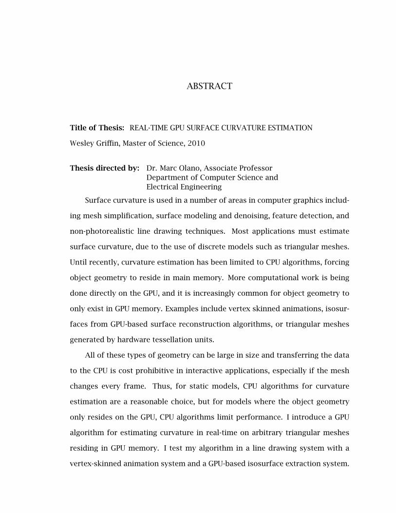
3.1 The left is a triangle containing vertex v2 with adjacent vertices. The
right is a one-ring neighborhood of faces around vertex v2. Notice that
adjacency information does not allow access to vertices v6 and v7 in
the one-ring. . . . . . . . . . . . . . . . . . . . . . . . . . . . . . . . . . . . . 22
v
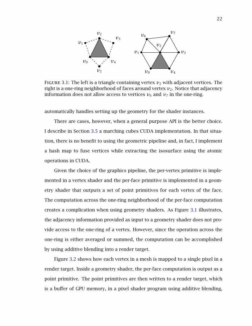
3.2 The contribution of the one-ring neighborhood of a vertex is averaged
by blending into a single pixel of a render target. A single vertex with
the one-ring of faces is indicated by the dashed circle. The same vertex
from each face is mapped as a point primitive to a single pixel of a
render target. The blue lines show a complete one-ring, while the red
and green lines show how other vertices could be mapped. . . . . . . . 23
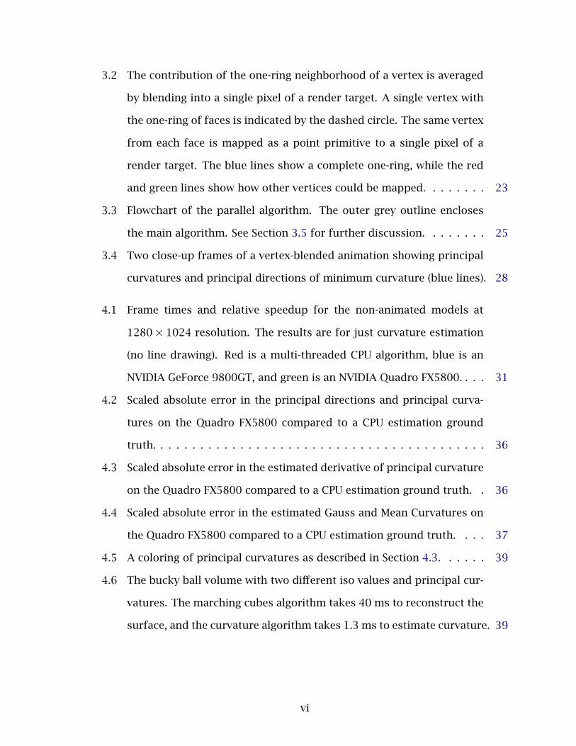
3.3 Flowchart of the parallel algorithm. The outer grey outline encloses
the main algorithm. See Section 3.5 for further discussion. . . . . . . . 25
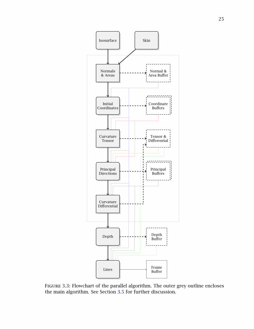
3.4 Two close-up frames of a vertex-blended animation showing principal
curvatures and principal directions of minimum curvature (blue lines). 28
4.1 Frame times and relative speedup for the non-animated models at
1280 × 1024 resolution. The results are for just curvature estimation
(no line drawing). Red is a multi-threaded CPU algorithm, blue is an
NVIDIA GeForce 9800GT, and green is an NVIDIA Quadro FX5800. . . . 31
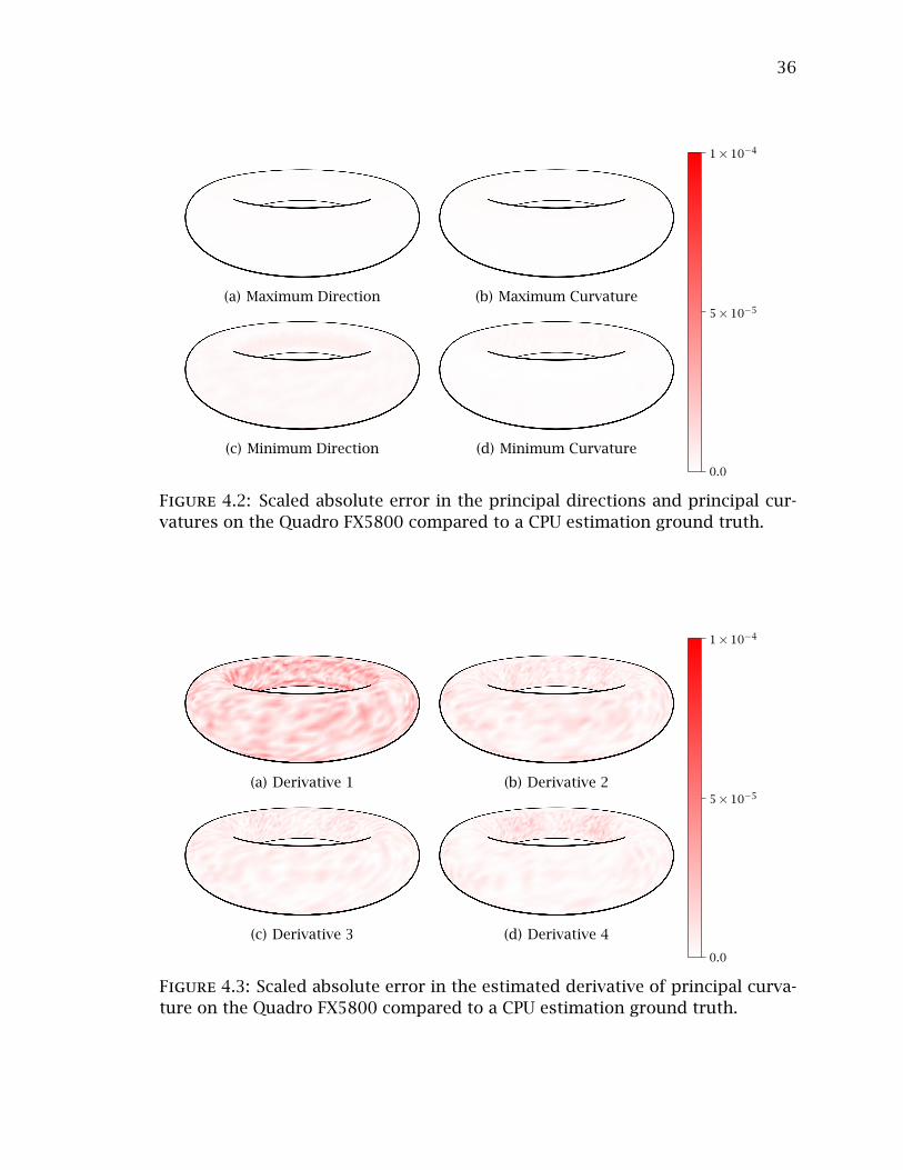
4.2 Scaled absolute error in the principal directions and principal curva-
tures on the Quadro FX5800 compared to a CPU estimation ground
truth. . . . . . . . . . . . . . . . . . . . . . . . . . . . . . . . . . . . . . . . . . 36
4.3 Scaled absolute error in the estimated derivative of principal curvature
on the Quadro FX5800 compared to a CPU estimation ground truth. . 36
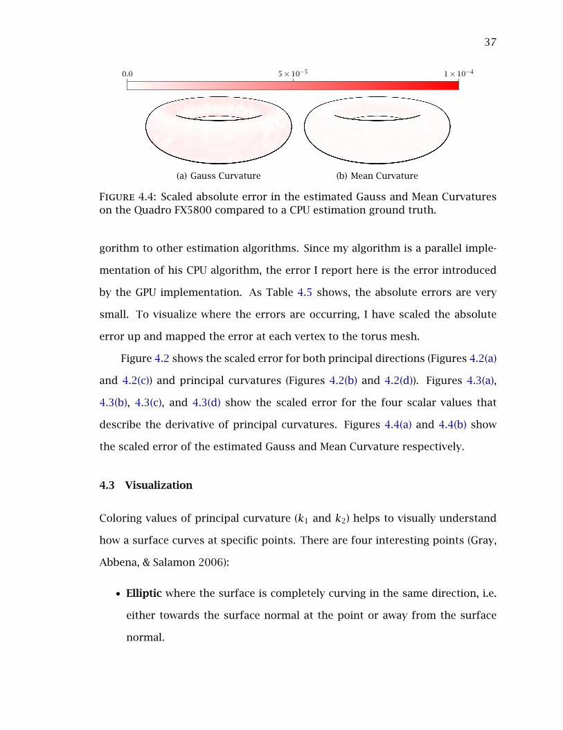
4.4 Scaled absolute error in the estimated Gauss and Mean Curvatures on
the Quadro FX5800 compared to a CPU estimation ground truth. . . . 37
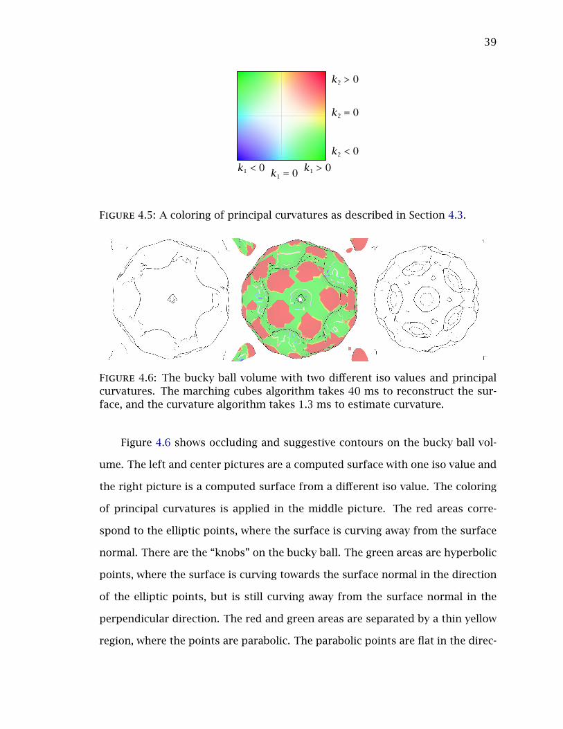
4.5 A coloring of principal curvatures as described in Section 4.3. . . . . . 39
4.6 The bucky ball volume with two different iso values and principal cur-
vatures. The marching cubes algorithm takes 40 ms to reconstruct the
surface, and the curvature algorithm takes 1.3 ms to estimate curvature. 39
vi

4.7 The heptoroid model with 286,678 vertices. The top left and middle
images show occluding and suggestive contours with lambertian shad-
ing, while the bottom left and right images show values of principal
curvature. . . . . . . . . . . . . . . . . . . . . . . . . . . . . . . . . . . . . . . 40
4.8 A sequence of frames from the camel model. The middle frame shows
principal directions and the last frame shows principal values of cur-
vatures. . . . . . . . . . . . . . . . . . . . . . . . . . . . . . . . . . . . . . . . 41
4.9 The animated horse model. The first two pictures show just the prin-
cipal curvatures. The last two pictures show the principal directions
of minimum (blue lines) and maximum (brown lines) curvature. . . . . 41
4.10 Principal curvatures on the high-quality elephant model. . . . . . . . . . 41
4.11 Looking into an extracted surface of the bucky ball volume with tone
shading. . . . . . . . . . . . . . . . . . . . . . . . . . . . . . . . . . . . . . . . 41
4.12 The orange volume with over 1.5B vertices. Curvature is estimated in
32.1 ms (31 fps) on this surface that is computed in 928 ms. . . . . . . 42
vii

LIST OF TABLES
3.1 Operations that can be performed in parallel grouped by their in-
put. The output is listed as well as whether it should be averaged
or summed across the one-ring neighborhood of a vertex. . . . . . . . . 18
3.2 Average valence of the models. . . . . . . . . . . . . . . . . . . . . . . . . . 19
4.1 Memory usage and CPU performance at 1280× 1024 resolution. RAM
is just the render targets and geometry buffers, while (Total) includes
a super-sampled depth buffer and other shared overhead. Algorithm
refers to a multi-threaded benchmark CPU algorithm. . . . . . . . . . . 32
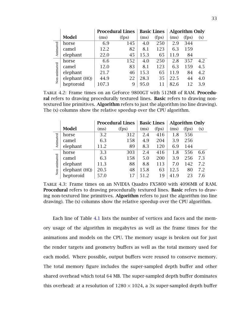
4.2 Frame times on an GeForce 9800GT with 512MB of RAM. Procedural
refers to drawing procedurally textured lines. Basic refers to drawing
non-textured line primitives. Algorithm refers to just the algorithm
(no line drawing). The (x) columns show the relative speedup over the
CPU algorithm. . . . . . . . . . . . . . . . . . . . . . . . . . . . . . . . . . . . 33
4.3 Frame times on an NVIDIA Quadro FX5800 with 4096MB of RAM. Pro-
cedural refers to drawing procedurally textured lines. Basic refers to
drawing non-textured line primitives. Algorithm refers to just the al-
gorithm (no line drawing). The (x) columns show the relative speedup
over the CPU algorithm. . . . . . . . . . . . . . . . . . . . . . . . . . . . . . 33
viii

4.4 Frame times for different volumes at 1280 × 1024 resolution on the
NVIDIA Quadro FX5800. I-V is the iso value of the surface and E-T is
the elapsed time to extract the surface. Lines refers to drawing non-
textured line primitives. Algorithm refers to just the algorithm (no
line drawing). . . . . . . . . . . . . . . . . . . . . . . . . . . . . . . . . . . . . 34
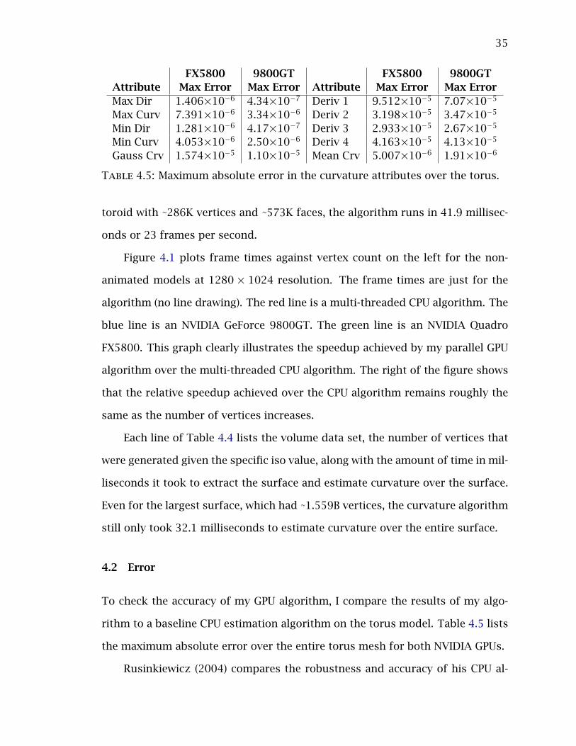
4.5 Maximum absolute error in the curvature attributes over the torus. . . 35
ix

chapter 1
INTRODUCTION
Surface curvature is used in a number of areas in computer graphics including
texture synthesis and shape representation, mesh simplification, surface mod-
eling, and artistic line drawing techniques. All of these techniques, which I de-
scribe next, operate on a discrete polygonal representation (almost always trian-
gular polygons) of a continuous surface, called a mesh or model.
Texture synthesis is a technique to generate a texture that seamlessly covers
a mesh from a small exemplar texture. Gorla et al. (2003) present a technique
that would use principal directions of curvature, provided reliable estimates
were available, to drive texture synthesis and affect shape recognition. Mesh
simplification attempts to create a new mesh that has fewer triangles than an
existing mesh, but that still resembles the approximated surface. An optimal
approximation to mesh simplification relies on surface curvature (Heckbert &
Garland 1999). Surface modeling, on the other hand, creates a smooth mesh
from a specified set of geometric constraints, which include surface curvature.
Moreton and Séquin’s (1992) algorithm minimizes the variation of curvature in
evaluating the smooth mesh.
1.1 Artistic Line Drawing
Most computer graphics image generation is concerned with generating realistic
images. Artistic line drawing techniques (Section 2.3) instead attempt to gen-
erate images that mimic an artistic style, such as pen-and-ink drawings or use
hatching to convey lighting and shading in generated images. Artistic techniques
1

2
are more commonly referred to as non-photorealistic rendering (NPR).
When drawing lines, there are a number of lines, or contours, that can be
drawn, many of which are based on curvature. The simplest form of contours,
occluding contours, do not depend on curvature. Occluding contours are the
set of points where the surface normal is perpendicular to the viewing direction.
When drawn, these contours form a silhouette around the mesh. Suggestive
contours (DeCarlo et al. 2003) use the derivative of curvature to draw “almost
contours”, which would be contours if the view was shifted slightly. Other types
of contours based on curvature are ridge and valley contours. These contours
are the set of points of local minimum or maximum curvature. Kolomenkin,
Shinshoni, and Tal (2008) use the gradient of curvature to locate the points of
inflection between ridges and valleys. Demarcating curves are the set of points
where the inflection is strongest.
Judd, Durand, and Adelson (2007) define view-dependent curvature by pro-
jecting curvature onto the viewing plane where the image is rendered (screen
space). They then define apparent ridges as the set of points of local minimum
or maximum view-dependent principal curvature.
1.2 Curvature
Intuitively, curvature describes how a curve turns as a particle moves along the
curve over time. On a surface, normal curvature (Section 2.1) describes how a
surface bends as a particle moves around the surface over time. Curvature, in
general, is defined on continuous surfaces. In computer graphics, however, only
a discrete polygonal representation of the continuous surface exists and must
be estimated.
Curvature estimation algorithms (Section 2.2) have traditionally been imple-
mented on general purpose CPUs, thereby forcing object geometry to reside in

3
main memory. This requirement was not considered a limitation as geometry
always resided in main memory. However, more computational work is being
performed directly on the graphics processing unit (GPU) and it is not unreason-
able for object geometry to only exist in GPU memory. I describe three cases
where geometry only exists on the GPU in the following section.
For static models, curvature only needs to be estimated once, so CPU algo-
rithms are a reasonable choice, but for deforming models, curvature must be
estimated every time the model changes. Estimating curvature every frame on
the CPU is expensive, especially if the geometry exists on the GPU and must be
transferred to the CPU. Algorithms do exist to estimate curvature in real-time
on deforming models. These methods either work in image-space (Kim et al.
2008) or require a pre-processing step to learn the curvature function on a train-
ing data set (Kalogerakis et al. 2009). While both techniques can be useful, the
ability to estimate curvature in object-space and without pre-processing training
data would provide much greater flexibility.
1.3 Computed Object Geometry
Below I present three cases where object geometry only exists in GPU memory:
vertex skinned animations used in video games, isosurfaces from GPU-based
surface reconstruction algorithms, and triangular meshes generated by hard-
ware tessellation units. In these situations, transferring the geometry off the
GPU to CPU memory to estimate curvature would be cost prohibitive.
Video games are starting to use non-photorealistic rendering techniques for
a more distinctive look (Mitchell, Francke, & Eng 2007; gearbox software 2009).
In most cases, these rendering techniques are applied to animated models that
move dynamically based on interaction with the user. Thus, these animated
models will change every frame and must be rendered in real-time. Video games

4
often use vertex-blended animations, also called vertex skinning, (Section 2.4) to
animate the models each frame. With vertex skinning, an initial pose mesh for
each model is transferred to the GPU just once. This pose mesh is then modified
each frame using blended transformation matrices to create an deformed mesh
corresponding to the animation for that frame. After skinning, the transformed
mesh only exists in GPU memory. Given the strict real-time requirements of
video games, transferring the vertex-blended animated models to the CPU to
estimate curvature is too costly.
GPU Computing, or General Purpose Computing on Graphics Hardware, ex-
ploits the massively parallel processing capability of modern graphics cards by
executing general purpose code on GPUs. This trend has increased the perfor-
mance of scientific simulation computations and visualizations. Typically, large
data sets are uploaded to the GPU and then a data-parallel algorithm is executed
over the data. Often, when working with volumetric data sets, these applications
need to visualize a surface re-constructed from the data set. I review surface
reconstruction in Section 2.5. As GPU memory capacity increases (workstation-
class cards currently have 4GB of RAM) GPUs can store higher resolution data
sets (greater numbers of polygons or larger dimension volumes) or more time
steps of time-varying data. Once the data set is uploaded to the GPU for com-
putation, transferring the data back to the CPU for surface reconstruction is
costly. In situations where an isosurface needs to be computed every time step
(for time-varying data) or recomputed interactively, reconstruction on a GPU can
offer improved performance for visualizing data in real-time. I describe a GPU
implementation of the marching cubes algorithm (Section 2.5) for surface recon-
struction in Section 3.5.1. After reconstruction, the surface only exists in GPU
memory and transferring the geometry to the CPU to estimate curvature would
be very expensive.

5
Tessellation is a process of refining a low-detail mesh (i.e. a mesh with a
small number of vertices) into a mesh that contains detailed geometric features.
Hardware tessellation units have existed for some time (Vlachos et al. 2001), but
with the introduction of the latest version of Microsoft’s Graphics API, DirectX
11 (Microsoft 2010), hardware-based tessellation is now part of a graphics pro-
gramming interface specification. For hardware tessellation, a low-detail mesh
is uploaded to the GPU and then tessellated, or subdivided, by the GPU. Video
games can benefit from hardware-based tessellation to enhance low-detail mod-
els in hardware. In these applications a potentially large triangular mesh will
likely be generated every frame and only exist in GPU memory.
1.4 Contributions
Estimating curvature with a CPU algorithm is a reasonable choice for static mod-
els, but in the case of deforming models or where the object geometry only exists
in GPU memory, estimating curvature on the CPU is too costly. Therefore, I in-
troduce a GPU algorithm for estimating curvature that works in object-space and
does not require any pre-processing or training data. Given an arbitrary trian-
gular mesh in GPU memory, the algorithm computes principal curvatures, prin-
cipal directions of curvature, the derivative of principal curvatures, and Gauss
and Mean curvatures at each vertex of the mesh in real-time. Since the algorithm
runs completely on the GPU and works on triangular meshes, it can be easily
adapted to existing rendering systems.
To demonstrate my algorithm I implemented a vertex-blending animation
system and a GPU-based isosurface extraction system, both of which use curva-
ture to extract and stroke occluding and suggestive contours on input data. My
algorithm runs in 41.9 ms (23 frames per second) on a model of 286,678 vertices
while estimating curvature every frame on the model. This is a speedup of 7.6

6
over an 8-core multi-threaded CPU implementation used as a benchmark. My
algorithm also runs in 21.1 ms (31 frames per second) on an isosurface recon-
struction containing 1,558,788 vertices while estimating curvature every frame.
My system can recompute the isosurface interactively, and computing this spe-
cific isosurface took 928 ms.
The specific contributions of this work are:
• A real-time GPU algorithm that computes principal curvatures, principal
directions of curvature, and the derivative of curvature.
• A marching cubes CUDA implementation that creates fused vertices.
Figure 1.1: Occluding and suggestive contours on a tone-shaded isosurface re-construction of a hydrogen atom volume.
The rest of this document is organized as follows: I discuss background
and related work in Chapter 2, describe the algorithm in detail in Chapter 3, and
present my results in Chapter 4.

chapter 2
BACKGROUND AND RELATED WORK
My system combines a number of components: curvature and curvature estima-
tion, line drawing, vertex-blended animation, and isosurface reconstruction.
2.1 Curvature
Below, I briefly discuss curvature and refer the reader to O’Neill (2006) for more
detail and relevant proofs of theorems.
At a point p on an oriented surface M, curvature describes how the tangent
plane, Tp(M), changes in different directions around p on M. An oriented surface
is a surface where a consistent direction for the normal vector at each point has
been chosen. For example, on a sphere, normals can point either inwards or
outwards, an oriented sphere is a sphere where the normals have been chosen to
point only in one direction. Surface normals are considered first-order structure
of smooth surfaces: at a point p, a normal vector Np defines a tangent plane
Tp(M) to a surface M. Figure 2.1 illustrates the tangent plane changing from one
point to another.
Curvature is typically defined in terms of the shape operator Sp(u), which is
the rate of change of a unit normal vector field, U in the direction u, where u is
a tangent vector to M at some point p:
(2.1) Sp(u) = −∇uU.
The shape operator is a symmetric linear operator, such that:
(2.2) S(u) · v = S(v) · u
7

8
pup
Np
Tp(M)
M
p'up'
Np'Tp
(M)
M
Figure 2.1: The tangent plane, Tp(M), to a surface M at two points p and p′.Curvature describes how the tangent plane changes from p to p′.
for any pair of tangent vectors u,v to M at p (O’Neill 2006).
Since the shape operator is a symmetric linear operator, it can be written
as a 2 × 2 symmetric matrix, S, for each point p given an orthonormal basis at
p. This symmetric matrix has real eigenvalues, λ1 and λ2 and eigenvectors, v1
and v2. The eigenvalues are called Principal Curvatures and the eigenvectors are
called Principal Directions.
Gauss Curvature, K, and Mean Curvature, H, can then be defined using the
eigenvalues:
K(p) = λ1λ2 = det S(2.3)
H(p) = 12(λ1 + λ2) = 1
2trace S(2.4)
Another way to describe curvature is normal curvature, k(u). There is a
theorem that relates normal curvature to the shape operator:
(2.5) k(u) = S(u) · u,
where u is a tangent vector to M at a point p. The maximum and minimum values
of k(u) at p are called principal curvatures, k1 and k2 and the directions in which

9
the maximum and minimum occur are called principal directions. Normal cur-
vature is second-order structure and effectively defines a quadric approximation
to M at p.
Traditionally, the second fundamental form is used to describe curvature,
and it can be defined in terms of the shape operator:
(2.6) II(u,v) = S(u) · v.
II is also called the curvature tensor and can be written using the directional
derivatives of normals (Rusinkiewicz 2004):
(2.7) II(u,v) =(Dun Dvn
)=
∂n∂u · u ∂n
∂v · u
∂n∂u · v ∂n
∂v · v
.
2.2 Curvature Estimation
On a discrete surface curvature must be estimated. There has been substantial
work in estimating surface curvature (Taubin 1995; Petitjean 2002; Goldfeather
& Interrante 2004; Rusinkiewicz 2004; Tong & Tang 2005). Gatzke and Grimm
(2006) divide the algorithms into three groups: surface fitting methods, dis-
crete methods that approximate curvature directly, and discrete methods that
estimate the curvature tensor (Equation 2.6). In the group that estimates the cur-
vature tensor, Rusinkiewicz (2004) and Theisel et al. (2004) estimate curvature
on a triangular mesh at each vertex by averaging the per-face curvature (calcu-
lated using surface normals and Equation 2.7) of each adjacent face to the vertex
(Figure 2.2). These algorithms have been limited to running on the CPU where
the algorithm can access faces adjacent to a vertex (the one-ring neighborhood
of the vertex).
Figure 2.3 shows directions and values of principal curvature estimated on a
triangular mesh representing a torus. The blue lines are directions of minimum

10
Figure 2.2: Estimating curvature using the directional derivatives of normalvectors (See Equation 2.7). The normal vectors at each vertex are shown in green,while the directions u and v are shown in blue.
curvature and, as expected on a torus, are flow around the torus, all in the same
direction. Likewise, the brown lines, which are directions of maximum curvature,
flow “up and down” the torus in the expected direction of maximum curvature.
The coloring legend helps to visually understand how the torus is curving at
specific points. For the torus, the red areas are “elliptic”, which is where the
surface is completely curving away from the surface normal at each point. The
green areas are “hyperbolic”, which is where the surface is curving away from
the normal in one direction and curving towards the normal in another direction.
The red and green areas are separated by a thin yellow area along the “top” and
“bottom” of the torus, where the surface is still curving in one direction, but flat
in another direction.
Recently Kim et al. (2008) introduced an image-based technique that esti-
mates curvature in real-time on the GPU. Their method traces rays based on the
normals at a point to estimate the direction of curvature.

11
k2 > 0
k2 = 0
k2 < 0
k1 < 0 k1 > 0k1 = 0
Figure 2.3: Directions and values of principal curvature on a torus. Blue linesshow the principal directions of minimum curvature and brown lines show theprincipal directions of maximum curvature. On the legend, k1 is maximum cur-vature and k2 is minimum curvature.
Kalogerakis et al. (2009) also present a real-time method for estimating cur-
vature specifically on animated models. Their method requires a mesh that is de-
forming according to some provided parameterization, such as per-frame trans-
formation matrices, as described in Section 2.4. They use a pre-processing step
that learns a mapping from the animation parameters to curvature attributes.
This pre-processing step must estimate curvature for each value of the param-
eterization, thus, for a vertex-skinned model, curvature will be estimated for
every frame. Once the mapping has been created, their algorithm predicts cur-
vature attributes in real-time given an unseen set of animation parameters.
One drawback of this approach is that the input data set must have a pa-
rameterization that can be used for the learning algorithm. Also, the method is
limited to the range of motions expressed in the animation parameter training
data set. If the training data does not cover motions that are part of the real-
time input data, the method will not be able to accurately predict the curvature
on those motions.
While the methods by Kim et al. (2008) and Kalogerakis et al. (2009) can be
useful, the ability to estimate curvature in object-space, without pre-processing,

12
and on unseen motions would provide greater flexibility in using curvature.
2.3 Line Drawing
Line drawing algorithms can be subdivided into two classes: image-based and
object-based. Image-based techniques rasterize the scene, sometimes multiple
times, and use image processing techniques to find surface properties and fea-
ture lines which are then drawn into the scene. The algorithms must estimate
curvature on the objects in the image. Image-based algorithms are easier to
implement than object-based methods but have some deficiencies. First, the al-
gorithm will have to handle neighboring pixels that are not part of the same
object. Second, the algorithms are limited to the resolution of the image and
cannot account for sub-pixel detail. Also, temporal coherence can be an issue
and the shower-door effect, where the lines appear to be drawn on the viewing
plane and not on the object (Meier 1996), must be managed. Finally, stylization
can be difficult as feature lines are not represented with geometry.
Object-based methods typically use second- and third-order surface prop-
erties to extract feature lines directly from a polygonal model in world-space.
Suggestive contours (DeCarlo et al. 2003), apparent ridges (Judd, Durand, &
Adelson 2007), and demarcating curves (Kolomenkin, Shimshoni, & Tal 2008)
are examples of object-based techniques. These algorithms can be divided into
two groups: view-dependent and view-independent. View-dependent methods
include the viewing direction when extracting feature lines, view-independent
methods do not. Both groups of techniques, however, rely on some method for
estimating curvature on a mesh.
Occluding, or silhouette, contours require normals (first-order structure),
apparent ridges require curvature (second-order structure), and suggestive con-
tours and demarcating curves require the derivative of maximum and minimum

13
(i.e. principal) curvatures (third-order structure).
2.4 Vertex Blended Animation
Vertex blended animation, also called vertex skinning, is an animation technique
where the vertices of a model are deformed each frame by a set of weighted
transformation matrices. Each vertex is assigned one or more bones along with
a weight for each bone assignment. For each frame, the vertices are transformed
using the weighted transformation matrices of the assigned bones.
This technique, often called linear blend skinning, is the most common
method used. Other techniques have been proposed, however, such as dual-
quaternion blending (Kavan et al. 2008). I have implemented linear blend skin-
ning to demonstrate the effectiveness of our algorithm, but do not make any
specific contribution to the area of vertex blended animation, and refer the
reader to existing excellent surveys (Akenine-Möller, Haines, & Hoffman 2008;
Jacka et al. 2007) for further discussion of vertex blended animation.
2.5 Isosurface Reconstruction
Surface reconstruction is one of the most frequently used methods to analyze
and visualize volumetric data. Marching cubes (Lorensen & Cline 1987) is the
most widely used algorithm for computing a triangular surface or model from
volumetric data. Treece et al. (1999) use a variation of marching cubes, marching
tetrahedra, that is easier to implement and handles non-gridded data. Geiss
(2007) introduces a marching cubes implementation using the programmable
graphics pipeline. To improve the speed of his implementation, he introduces a
method for pooling vertices and creating an indexed triangle list. My algorithm
does require shared vertices, however, Geiss’ method is limited to a fixed voxel

14
size. In Section 3.5, I introduce a CUDA implementation of marching cubes that
uses a hash map to fuse vertices.
2.6 Graphics Hardware
Graphics hardware has evolved considerably over the last decade. Modern GPUs
are massively parallel programmable units. Below, I describe the architecture of
modern GPUs and then discuss their programmability.
2.6.1 Architecture
Graphics processing units were initially introduced as fixed-function hardware
implementations of the graphics pipeline. Over the last decade, different stages
of the pipeline have become programmable (Section 2.6.2). As more stages
became programmable, GPU architectures evolved into a more general Single-
Instruction Multiple-Data (SIMD) (Flynn 1972) architecture, with a unified archi-
tecture implementing a “common-core” Application Programming Interface (API)
(Blythe 2006).
The unified architecture of modern GPUs uses many small, lightweight vec-
tor processing units. The processing units are grouped into cores which share a
small local memory store. Each processing unit also has access to a larger global
Vertex Geometry Rasterization
Memory
Pixel Merge
Figure 2.4: The modern programmable graphics pipeline. The shaded stagesare programmable, while the non-shaded stages are highly configurable.

15
memory. The programs (shaders) corresponding to the programmable stages of
the pipeline are executed on the processing units.
To hide memory latency, a hardware scheduler attempts to maximize the
utilization of the processors by scheduling many independent programs on the
processing units and using very fast context switching to switch between the
programs. The combination of hardware scheduling and fast context switching
allows a GPU to reassign processors and shuffle data around very efficiently,
especially compared to large-scale computing clusters such as the Roadrunner
supercomputer (Barker et al. 2008).
2.6.2 Programmability
Olano and Lastra (1998) introduced the first system capable of real-time pro-
cedural shading in hardware. Lindholm et al. (2001) presented the first pro-
grammable vertex shader on a GPU. Proudfoot et al. (2001) introduced pro-
grammable vertex and pixel shader stages. Blythe (2006) added an additional
stage to the programmable pipeline: the geometry shader stage. This stage op-
erates on entire primitives and can access every vertex of an input primitive.
GPUs are ideally suited to executing data-parallel algorithms. Data-parallel
algorithms execute identical units of work (programs) over large sets of data.
The algorithms can be parallelized for efficiency when the work units are inde-
pendent and are able to run on small divisions on the data. One critical aspect
of designing parallel algorithms is identifying the units of work and determining
how they will interact via communication and synchronization. A second critical
aspect is analyzing the data access patterns of the programs and ensuring data
locality to the processing units. A final factor is scheduling the programs to run
on hardware and moving the data to where the programs will execute (Almasi &
Gottlieb 1994).

16
In a cluster supercomputer, parallel processes run simultaneously and com-
municate through shared memory or message passing. Since the GPU uses pro-
cess scheduling to increase efficiency (Section 2.6.1), two processes that want to
communicate may not even be running at the same time. To allow communi-
cation, the GPU programmer introduces barriers defined by passes (or kernels).
Results written by one kernel (or pass) can be randomly accessed in the next.
Thus, the defining feature of parallel algorithm design for the GPU is not as
much data assignment to processors as the selection of passes/kernels and syn-
chronization points.

chapter 3
PARALLEL ALGORITHM
My algorithm is based on the CPU algorithm by Rusinkiewicz (2004). In his
algorithm, Rusinkiewicz creates a set of linear constraints to solve for curvature
(Equation 2.7) over a single face. The constraints use the differences between
normals along edges and are solved using least squares. To find the curvature
at a vertex, the per-face curvatures of each adjacent face are averaged together.
The algorithm is composed of several iterative steps that can be grouped
based on the type of input to each step: either per-face or per-vertex. While each
step builds on the computation from the previous step, within each step the
computation is independent over each subdivision on the input. That is, a per-
face step works on a single face and a per-vertex step works on a single vertex.
My parallel algorithm exploits this independence of computation to parallelize
the work within each step.
Table 3.1 summarizes the iterative steps listed below, grouping them based
on the type of input to each step.
1. Normals. Normals at each vertex are computed by averaging the per-face
normals of the one-ring.
2. Areas. A weighting is calculated to determine how much a face contributes
to each of the three vertices.
3. Initial Coordinates. An orthonormal basis is generated at each vertex. This
basis is used to transform the curvature tensor at each vertex.
4. Curvature Tensor. An over-specified linear system for the tensor of a face
17

18
Input Operation Output One-Ring
Face
Normals Vector AveragedAreas Scalar Summed
Initial Coordinates 2 Vectors NoCurvature Tensor 3 Scalar Values Averaged
Curvature Differential 4 Scalar Values AveragedVertex Principal Directions 2 Vectors & No
& Principal Curvatures 2 Scalar Values
Table 3.1: Operations that can be performed in parallel grouped by their input.The output is listed as well as whether it should be averaged or summed acrossthe one-ring neighborhood of a vertex.
is created from the differences of normals along the edges of the face and
solved using LDLT decomposition and least squares fit. The tensor is ro-
tated into a local coordinate system at each vertex using the orthonormal
basis and weighted by the area of the vertex. These weighted tensors at
each vertex are summed across the one-ring to compute the averaged cur-
vature tensor at each vertex.
5. Principal Directions. The Jacobi method is then used to diagonalize the
curvature tensor at each vertex and approximate eigenvalues and eigen-
vectors and thus compute principal curvatures and directions.
6. Principal Curvatures Differential. The principal curvatures at each vertex
are used to find the differential of principal curvatures by solving a set of
linear constraints per face and averaging across the one-ring.
3.1 Complexity Analysis
The steps described above are all composed of mathematical operations, loading
and storing values to memory locations, and fixed-length loops (either three or
four iterations). Thus the CPU algorithm is linear in the size of the input. Five of

19
AverageModel Valencetorus 6.0000horse 5.9932camel 6.0055elephant 5.9997elephant (HQ) 5.9839heptoroid 6.0009
Table 3.2: Average valence of the models.
the six steps operate on faces, while the sixth step operates on vertices, so the
input size depends on the step.
Given a model with n vertices, the number of faces, f can be approximated:
(3.1) f ≈ n∗ V3
,
where V is the average valence of the model. The valence of a vertex is the
number of edges connected to the vertex, so the average valence of a model is
the sum of the valences at each vertex divided by the total number of vertices
in the model. Table 3.2 lists the average valence for the set of models that I
describe in Chapter 4.
In Equation 3.1, each vertex is, on average, connected to V faces. Each face,
however, is shared by three vertices and this fact is accounted for by the division.
Since the steps in Table 3.1 are iterative, the running time, T(n), of the CPU
algorithm on a model with n vertices and constant average valence V is the sum
of the running times of each step:
T(n) = O(f)+O(f)+O(f)+O(f)+O(f)+O(n)
= 5∗O(n∗ V
3
)+O(n)
= O(n)
(3.2)

20
3.2 Parallel Considerations
As discussed in Section 2.6, data locality is critical to algorithm efficiency and
hardware utilization. The steps discussed above all use only the local data of a
face or vertex. Thus, parallel implementations of each step should be efficient
as the memory access pattern of each step is localized.
In addition to grouping the steps based on the type of input, Table 3.1 lists
the type of output and whether the output must be averaged or summed across
the one-ring neighborhood of a vertex for each step. Except for the Principal
Directions & Principal Values step, the output from each step will fit into a
four-component vector. Again, this means parallel implementations of each
step should be efficient, as GPUs are optimized for writing to buffers of four-
component vectors, and each step can write to a single output buffer.
The Principal Directions & Principal Values step outputs two vectors, one
for each principal direction of curvature, and two scalar values, one for each
principal curvature. The scalars can be combined with their respective vectors
and thus this step will require two output buffers.
3.3 Computational Primitives
Based on Table 3.1 and the previous discussion, I define two computational prim-
itives to implement the parallel algorithm:
1. A per-vertex primitive that takes a single vertex as input, and outputs a
computation at the vertex.
2. A per-face primitive that takes a single face (composed of three vertices)
as input, and outputs a computation at each vertex of the face that will be
averaged or summed across the one-ring neighborhood.

21
In a parallel algorithm, the data parallel threads will be distributed across
both processors and time. Data written by one thread that will be read in another
thread must force a barrier for all threads to complete. In my algorithm, the per-
vertex computations are independent and thus need no barrier between other
threads. However, since the per-face computations are averaged or summed
across multiple threads, a barrier is required.
3.4 Primitive Implementation
There are two possibilities for implementing the computational primitives: the
graphics pipeline, using shaders, or the general purpose APIs such as Compute
Unified Device Architecture (CUDA) (NVIDIA 2009). Functionally, both choices
are equivalent, they each execute on the same hardware. The primary differences
in the approaches relative to this work are more flexible shared memory access
in CUDA and special purpose hardware for blending in the graphics pipeline.
The algorithm needs to sum across several threads, which could be accom-
plished with a CUDA atomic add or graphics pipeline blending. In either case a
pass or kernel barrier must be introduced before using the results. The writes
to the output buffers cannot be constrained to a single thread block, so a CUDA
implementation would need a full kernel synchronization point, not just the
lighter-weight syncthreads barrier. In contrast, GPUs have special hardware for
blending to output buffers (render targets) with dedicated Arithmetic Logic Units
(ALUs), optimized for throughput.
Curvature estimation is a geometric problem, treating it as such, i.e. using
the geometric pipeline, allows use of the more efficient blending hardware to
synchronize access instead of atomic operations accompanied by an immediate
kernel end. Additionally, when the geometry already exists in a format that
the graphics pipeline expects (i.e. indexed vertex buffers), using the pipeline
22
v0
v1
v2
v3
v4
v6v7
v0
v1
v2v3
v4
v5
Figure 3.1: The left is a triangle containing vertex v2 with adjacent vertices. Theright is a one-ring neighborhood of faces around vertex v2. Notice that adjacencyinformation does not allow access to vertices v6 and v7 in the one-ring.
automatically handles setting up the geometry for the shader instances.
There are cases, however, when a general purpose API is the better choice.
I describe in Section 3.5 a marching cubes CUDA implementation. In that situa-
tion, there is no benefit to using the geometric pipeline and, in fact, I implement
a hash map to fuse vertices while extracting the isosurface using the atomic
operations in CUDA.
Given the choice of the graphics pipeline, the per-vertex primitive is imple-
mented in a vertex shader and the per-face primitive is implemented in a geom-
etry shader that outputs a set of point primitives for each vertex of the face.
The computation across the one-ring neighborhood of the per-face computation
creates a complication when using geometry shaders. As Figure 3.1 illustrates,
the adjacency information provided as input to a geometry shader does not pro-
vide access to the one-ring of a vertex. However, since the operation across the
one-ring is either averaged or summed, the computation can be accomplished
by using additive blending into a render target.
Figure 3.2 shows how each vertex in a mesh is mapped to a single pixel in a
render target. Inside a geometry shader, the per-face computation is output as a
point primitive. The point primitives are then written to a render target, which
is a buffer of GPU memory, in a pixel shader program using additive blending,

23
∑
A
BC
D
EF
Figure 3.2: The contribution of the one-ring neighborhood of a vertex is aver-aged by blending into a single pixel of a render target. A single vertex with theone-ring of faces is indicated by the dashed circle. The same vertex from eachface is mapped as a point primitive to a single pixel of a render target. The bluelines show a complete one-ring, while the red and green lines show how othervertices could be mapped.
where the current value in the shader is added to the existing value in the target.
Using this technique, the algorithm can easily average or sum values of the one-
ring neighborhood around a vertex. While this mapping technique requires input
meshes with fused vertices, in practice, fusing vertices is not a difficult task. In
Section 3.5 I discuss fusing vertices when extracting isosurfaces.
3.5 Parallel Instances
Figure 3.3 is a flowchart of the parallel algorithm, where the outer grey outline
surrounds the actual algorithm. Since each step of the algorithm described in
Section 3 builds on the computation from the previous step, synchronization
points between each step of the algorithm are necessary. Render passes are
natural synchronization points and since the one-ring computation uses additive
blending to a render target, the synchronization barrier between each step is a
pass through the pipeline.
Each pass of the parallel algorithm is shown on the left with the correspond-

24
ing output render targets on the right. Each render target is connected to the
subsequent passes that use the buffer as input. Each pass is an instance of one of
the computational primitives described in Section 3.3. In Figure 3.3, the passes
with square corners average or sum the output over the one-ring neighborhood,
while the passes with round corners do not.
To demonstrate the algorithm, I have implemented a GPU-based isosurface
extraction system and a vertex-blending animation system, both of which use
curvature to extract and stroke occluding and suggestive contours on input data.
To support the two types of input: volumetric datasets and skinned anima-
tions or static models, I have two initial passes that either compute an isosurface
for a volumetric dataset (Isosurface) or animate the vertices using vertex skin-
ning (Skin). If a static model, i.e. a triangular mesh with no animation, is input,
the Skin pass is still used.
After transforming the input, the iterative steps of the algorithm are run.
Once the algorithm has completed, I use the curvature results to extract and
stroke contours on the input data. To ensure high-quality contour stroking, I
compute a super-sampled depth buffer in the Depth pass.
I describe these steps as well as each step of the algorithm below.
3.5.1 Isosurface
To demonstrate occluding and suggestive contours on volumetric datasets, I first
compute an isosurface from the input data. This pass is a standard CUDA march-
ing cubes implementation to compute an isosurface over the volume. However,
since the parallel curvature algorithm requires shared vertices to map the one-
ring around each vertex (Section 3.4), I modify the algorithm to output an in-
dexed, fused triangle list.
After classifying the voxels and determining how many vertices are needed
25
Isosurface Skin
Normals& Areas
Normal &Area Buffer
InitialCoordinates
CoordinateBuffers
CurvatureTensor
Tensor &Differential
PrincipalDirections
PrincipalBuffers
CurvatureDifferential
Depth DepthBuffer
LinesFrameBuffer
Figure 3.3: Flowchart of the parallel algorithm. The outer grey outline enclosesthe main algorithm. See Section 3.5 for further discussion.
26
for each active voxel, two sequential kernels are run: a triangle kernel and an
index kernel. The triangle kernel generates the vertex buffer along with a “full”
index buffer, where every vertex is separately indexed and the index kernel gen-
erates the final index buffer, containing only shared indices.
Each instance of the triangle kernel will create anywhere from zero to twelve
vertices. When a vertex is created, three arrays are filled in: the vertex buffer with
the actual vertex, the “full” index buffer, and a hash code buffer with the hash
code of the vertex. Using radix sort (Satish, Harris, & Garland 2009), I sort the
hash code and index buffers as key/value pairs.
The index kernel then re-creates the vertices and hash codes and, for each
vertex, uses binary search to locate the first index of the current vertex in the
vertex buffer. Since there may be duplicate keys, once the binary search termi-
nates, if a match was found, the search algorithm traverses backwards in the
key buffer until the first hash code is located. To resolve collisions in the hash
function, after locating a match, the kernel traverses forwards in the key buffer,
comparing the corresponding value in the vertex buffer with the current vertex.
Once the kernel has located the first vertex in the vertex buffer that matches the
current vertex, it writes the corresponding index to an final, fused index buffer.
3.5.2 Skin
To demonstrate occluding and suggestive contours on skinned animations or
static models, I use a vertex shader to skin each vertex based on the current
set of keyframe matrices as described in Section 2.4. In the case of a static, or
non-animated, model, the output vertex position is the same as the input vertex
position. The deformed vertices are written to a new buffer in GPU memory
using the stream out mechanism (Blythe 2006).

27
3.5.3 Normals & Areas
The curvature algorithm requires high quality normals at each vertex in the
mesh. Since my input data could be changing each frame, this pass re-calculates
a normal and an area for each vertex of a face in a geometry shader. To start,
the geometry shader calculates a face normal for each triangle in the mesh. The
normal at a vertex is the weighted average of face normals across the one-ring
of the vertex. Like Rusinkiewicz (2004), the area at a vertex is the Voronoi area
described by Meyer et al. (2003) and is used in later passes to weight the con-
tribution of each face to the vertices that compose the face. Using the one-ring
computation technique described in Section 3.3, the face normals of the one-ring
at a vertex are averaged together and the areas of the one-ring are summed.
Since the normal is a three-component floating point vector and the area is
a floating point scalar value, both the normal vector and area scalar are packed
into a single four-channel render target.
3.5.4 Initial Coordinates
An orthonormal basis is required at each vertex to transform the curvature ten-
sor of a face into a local coordinate system. The basis is computed using a
geometry shader and each vector is written to a separate four-channel render
target.
While it would seem that the basis could be created as needed in any later
passes, each vertex needs a single basis so that all of the per-face curvature
tensor transformations happen in the same coordinate system. If the bases were
computed on the fly, then each face attached to the same vertex would use a
different basis based on that face. Thus, this separate pass computes a single,
constant basis for each vertex based on a single face.

28
3.5.5 Curvature Tensor
Before computing principal directions and principal curvatures, my algorithm
must estimate the curvature tensor at each vertex in the mesh. I use a geometry
shader to compute the curvature tensor at each face (Equation 2.7). For each
edge, the shader computes the differences of normals along the edges. A linear
system for the tensor is created from those differences and a solution is found
using least squares. Using the one-ring computation technique, the weighted
tensor at each face is averaged across the one-ring to compute the curvature
tensor at a vertex. The tensor is three floating point values and is stored in a
four-channel render target.
3.5.6 Principal Directions
I use a vertex shader to compute the minimum and maximum curvatures and
principal directions at each vertex. Since this pass only needs to execute over a
single vertex, no geometry shader is used and no blending is used in the pixel
shader. The minimum curvature and principal direction are packed into one
four-channel buffer and a second four-channel buffer is used for maximum cur-
vature and principal direction.
Figure 3.4 shows principal curvatures and direction of minimum curvature
k2 > 0
k2 = 0
k2 < 0
k1 < 0 k1 > 0k1 = 0
Figure 3.4: Two close-up frames of a vertex-blended animation showing princi-pal curvatures and principal directions of minimum curvature (blue lines).

29
(blue lines) from this pass in two consecutive frames of an animation. In the
first frame, the large red area is where the shin is bent such that the surface
is curving away from the surface normal at each point. As the shin straightens
in the second frame, the red area shrinks and is replaced by portions of green,
where the surface is curving away from the surface normal in one direction and
curving towards the surface normal in another direction at each point. Coloring
principal curvatures is discussed further in Section 4.3.
3.5.7 Curvature Differential
Suggestive contours (DeCarlo et al. 2003) and demarcating curves (Kolomenkin,
Shimshoni, & Tal 2008) both require the derivatives of principal curvatures.
Not all curvature estimation algorithms can generate these derivatives, however
Rusinkiewicz’s method is able to estimate them and thus my parallel algorithm
is able to estimate them as well.
I use a geometry shader to compute the derivative of principal curvatures
using the same process as the Curvature Tensor pass. The derivative is essen-
tially a third-order property, incorporating information from a two-ring around
the vertex (i.e. a one-ring of data computed on a one-ring around a vertex). Thus,
the variation of principal curvatures along the edge of a face is used instead of
using the variation of normals. These per-face differentials are averaged over the
one-ring of faces. The derivative of principal curvatures is represented with a
four-component floating point value. The output of the Curvature Tensor pass is
no longer needed at this point, so the Tensor & Differential four-channel render
target is reused for this pass.

30
3.6 Depth
To improve the quality of the stroke contours, I create a super-sampled depth
buffer for high-quality visibility testing in this pass. This depth buffer is used
only for line drawing and does not affect the curvature estimation. All curvature
computations happen at the polygon or vertex level in object space and the
quality of the estimation is not affected by any image or depth buffer resolution.
3.7 Drawing Lines
The final goal of my system is to extract and stoke occluding and suggestive con-
tours on the input data (either volumetric datasets or animated models). Once
the curvature algorithm has run, the Principal Buffers and Tensor & Differen-
tial Buffer are used, along with a super-sampled Depth Buffer, to extract feature
lines on the model. Lines are extracted in segments that are created per-face in a
geometry shader program. Currently my system extracts occluding and sugges-
tive contours. Line segments are created in the geometry program in one of two
ways: either as line primitives that are rasterized by the hardware, or as triangle
strips that can then be textured for stylized strokes.
When extracting line segments in the geometry shader, a global parameteri-
zation cannot be applied. Since the geometry program extracts only a single line
segment across a face, the program has no knowledge of where in the feature
line the segment is or how long the segment is. Also, since the line segments re-
side on the GPU, globally traversing the set of segments is extremely inefficient.
Thus, a stylization of the lines must not rely on any parameterization or global
access to the line, but can use 3D positions and procedural noise methods to
add stylization much like Johnston’s woodblock shader (2000) or Freudenberg’s
stroke textures (2002).

chapter 4
RESULTS
I discuss three types of results: performance, error, and visualization. Section
4.1 shows the actual performance of my GPU algorithm as well as a speedup
comparison to a baseline CPU algorithm. Section 4.2 compares the absolute
error of my GPU algorithm to a baseline CPU algorithm. Section 4.3 describes
the methods used to visualize the curvature results.
4.1 Performance
Tables 4.1, 4.2, 4.3, 4.4 along with Figure 4.1 show that my parallel algorithm
achieves real-time performance for small- to medium-sized models, even on
an older-generation consumer GPU. Results are shown for two different NVIDIA
Fram
eT
ime
(ms)
0
70
140
210
280
350
Vertices (1K)
0 100 200 300
Rel
ativ
eSp
eed
up
0123456789
10
Vertices (1K)
8.5 22 42.5 95 286.5
Figure 4.1: Frame times and relative speedup for the non-animated models at1280 × 1024 resolution. The results are for just curvature estimation (no linedrawing). Red is a multi-threaded CPU algorithm, blue is an NVIDIA GeForce9800GT, and green is an NVIDIA Quadro FX5800.
31

32
Memory (Total) AlgorithmModel Vertices Faces (MB) (MB) (ms) (fps)
An
imat
ed horse 8,431 16,843 5.8 (69.7)camel 21,887 43,814 17.5 (81.3)elephant 42,321 84,638 28.0 (91.8)
Non
-an
imat
ed
horse 8,431 16,843 5.6 (69.4) 11.8 85camel 21,887 43,814 16.8 (80.6) 28.3 35elephant 42,321 84,638 26.6 (90.4) 50.4 20elephant (HQ) 78,792 157,160 62.9 (126.7) 90.1 11heptoroid 286,678 573,440 238.3 (302.1) 318.6 3
Table 4.1: Memory usage and CPU performance at 1280×1024 resolution. RAMis just the render targets and geometry buffers, while (Total) includes a super-sampled depth buffer and other shared overhead. Algorithm refers to a multi-threaded benchmark CPU algorithm.
GPUs, an older-generation consumer-oriented card (GeForce 9800GT with 512MB
of RAM) and a high-end, workstation-class card (Quadro FX5800 with 4GB of
RAM). For these results, small-sized models have less than 50,000 vertices and
medium-sized models have between 50,000 and 300,000 vertices.
To benchmark the algorithm, I took an existing CPU algorithm and threaded
it to run in parallel. The CPU algorithm was run on a Core2 Quad Q8200 work-
station with 8GB of RAM and each core running at 2.33GHz. The Intel Threading
Building Blocks (TBB) (Intel 2010) library provides a number of multi-threaded
constructs, one of which is a parallel_for. The parallel_for construct takes a
function and a range describing the data set that will be operated on. TBB then
divides the work among a number of threads and executes the specified func-
tion on each thread over the subset of data. By default, TBB creates a number
of threads equal to the number of processors (or cores) and I used this default
to execute each step of the CPU algorithm over the four cores of the worksta-
tion. To synchronize thread access to shared data, I used a concurrent_vector,
also part of TBB, to store the data set. After trying several methods, I found the
combination of the TBB parallel_for and concurrent_vector to be the fastest.
33
Procedural Lines Basic Lines Algorithm OnlyModel (ms) (fps) (ms) (fps) (ms) (fps) (x)
An
imat
ed horse 6.9 145 4.0 250 2.9 344camel 12.2 82 8.1 123 6.3 159elephant 22.0 45 15.3 65 11.9 84
Non
-an
imat
ed
horse 6.6 152 4.0 250 2.8 357 4.2camel 12.0 83 8.1 123 6.3 159 4.5elephant 21.7 46 15.3 65 11.9 84 4.2elephant (HQ) 44.9 22 28.3 35 22.5 44 4.0heptoroid 107.3 9 95.0 11 82.6 12 3.9
Table 4.2: Frame times on an GeForce 9800GT with 512MB of RAM. Procedu-ral refers to drawing procedurally textured lines. Basic refers to drawing non-textured line primitives. Algorithm refers to just the algorithm (no line drawing).The (x) columns show the relative speedup over the CPU algorithm.
Procedural Lines Basic Lines Algorithm OnlyModel (ms) (fps) (ms) (fps) (ms) (fps) (x)
An
imat
ed horse 3.2 312 2.4 416 1.8 556camel 6.3 158 4.9 204 3.9 256elephant 11.2 89 8.3 120 6.9 144
Non
-an
imat
ed
horse 3.3 303 2.4 416 1.8 556 6.6camel 6.3 158 5.0 200 3.9 256 7.3elephant 11.3 88 8.8 113 7.0 142 7.2elephant (HQ) 20.5 48 15.8 63 12.5 80 7.2heptoroid 57.0 17 51.2 19 41.9 23 7.6
Table 4.3: Frame times on an NVIDIA Quadro FX5800 with 4096MB of RAM.Procedural refers to drawing procedurally textured lines. Basic refers to draw-ing non-textured line primitives. Algorithm refers to just the algorithm (no linedrawing). The (x) columns show the relative speedup over the CPU algorithm.
Each line of Table 4.1 lists the number of vertices and faces and the mem-
ory usage of the algorithm in megabytes as well as the frame times for the
animations and models on the CPU. The memory usage is broken out for just
the render targets and geometry buffers as well as the total memory used for
each model. Where possible, output buffers were reused to conserve memory.
The total memory figure includes the super-sampled depth buffer and other
shared overhead which total 64 MB. The super-sampled depth buffer dominates
this overhead: at a resolution of 1280× 1024, a 3x super-sampled depth buffer

34
I-V E-T Lines AlgorithmModel Vertices (ms) (ms) (fps) (ms) (fps)
bucky 43,524 0.2 40 2.1 476 1.3 769H atom 113,256 0.095 88 3.7 270 2.7 370spheres 302,688 0.2 232 9.1 110 6.8 147spheres 436,688 0.11 264 13.0 77 9.1 110orange 1,156,998 0.2 1088 33.4 30 25.2 40orange 1,558,788 0.15 928 43.9 23 32.1 31
Table 4.4: Frame times for different volumes at 1280 × 1024 resolution on theNVIDIA Quadro FX5800. I-V is the iso value of the surface and E-T is the elapsedtime to extract the surface. Lines refers to drawing non-textured line primitives.Algorithm refers to just the algorithm (no line drawing).
(3840 × 3072 samples) uses 47 MB. Since current GPUs have at least 512MB of
RAM, even the heptoroid model fits within the memory of a current GPU.
Each line of Tables 4.2 and 4.3 lists the frame times for the animations
and models on the GeForce 9800GT and the Quadro FX5800 respectively. The
Procedural Lines column lists the frame time in milliseconds for using proce-
durally generated line textures. The Basic Lines column lists the frame time in
milliseconds for using simple line primitives. The Algorithm Only column lists
the frame time in milliseconds for running just the algorithm along with the
speedup achieved over the benchmark CPU algorithm (the (x) column).
The top three entries of Tables 4.1, 4.2, and 4.3 are small- to medium-sized
animated models, while the middle three entries are the same models without
the animation. Comparing the animated results with the corresponding non-
animated results, the frame times are very close, most within 0.1 milliseconds.
The additional step of skinning models for animation adds very little runtime
to the algorithm. The bottom two entries are large, high-quality models with no
animation.
The times on the NVIDIA Quadro FX5800 indicate that the algorithm scales
well with increasing hardware resources. Even on the largest model, the hep-
35
FX5800 9800GT FX5800 9800GTAttribute Max Error Max Error Attribute Max Error Max ErrorMax Dir 1.406×10⁻⁶ 4.34×10⁻⁷ Deriv 1 9.512×10⁻⁵ 7.07×10⁻⁵
Max Curv 7.391×10⁻⁶ 3.34×10⁻⁶ Deriv 2 3.198×10⁻⁵ 3.47×10⁻⁵
Min Dir 1.281×10⁻⁶ 4.17×10⁻⁷ Deriv 3 2.933×10⁻⁵ 2.67×10⁻⁵
Min Curv 4.053×10⁻⁶ 2.50×10⁻⁶ Deriv 4 4.163×10⁻⁵ 4.13×10⁻⁵
Gauss Crv 1.574×10⁻⁵ 1.10×10⁻⁵ Mean Crv 5.007×10⁻⁶ 1.91×10⁻⁶
Table 4.5: Maximum absolute error in the curvature attributes over the torus.
toroid with ˜286K vertices and ˜573K faces, the algorithm runs in 41.9 millisec-
onds or 23 frames per second.
Figure 4.1 plots frame times against vertex count on the left for the non-
animated models at 1280 × 1024 resolution. The frame times are just for the
algorithm (no line drawing). The red line is a multi-threaded CPU algorithm. The
blue line is an NVIDIA GeForce 9800GT. The green line is an NVIDIA Quadro
FX5800. This graph clearly illustrates the speedup achieved by my parallel GPU
algorithm over the multi-threaded CPU algorithm. The right of the figure shows
that the relative speedup achieved over the CPU algorithm remains roughly the
same as the number of vertices increases.
Each line of Table 4.4 lists the volume data set, the number of vertices that
were generated given the specific iso value, along with the amount of time in mil-
liseconds it took to extract the surface and estimate curvature over the surface.
Even for the largest surface, which had ˜1.559B vertices, the curvature algorithm
still only took 32.1 milliseconds to estimate curvature over the entire surface.
4.2 Error
To check the accuracy of my GPU algorithm, I compare the results of my algo-
rithm to a baseline CPU estimation algorithm on the torus model. Table 4.5 lists
the maximum absolute error over the entire torus mesh for both NVIDIA GPUs.
Rusinkiewicz (2004) compares the robustness and accuracy of his CPU al-
36
(a) Maximum Direction (b) Maximum Curvature
(c) Minimum Direction (d) Minimum Curvature
0.0
5× 10⁻⁵
1× 10⁻⁴
Figure 4.2: Scaled absolute error in the principal directions and principal cur-vatures on the Quadro FX5800 compared to a CPU estimation ground truth.
(a) Derivative 1 (b) Derivative 2
(c) Derivative 3 (d) Derivative 4
0.0
5× 10⁻⁵
1× 10⁻⁴
Figure 4.3: Scaled absolute error in the estimated derivative of principal curva-ture on the Quadro FX5800 compared to a CPU estimation ground truth.
37
0.0 5× 10⁻⁵ 1× 10⁻⁴
(a) Gauss Curvature (b) Mean Curvature
Figure 4.4: Scaled absolute error in the estimated Gauss and Mean Curvatureson the Quadro FX5800 compared to a CPU estimation ground truth.
gorithm to other estimation algorithms. Since my algorithm is a parallel imple-
mentation of his CPU algorithm, the error I report here is the error introduced
by the GPU implementation. As Table 4.5 shows, the absolute errors are very
small. To visualize where the errors are occurring, I have scaled the absolute
error up and mapped the error at each vertex to the torus mesh.
Figure 4.2 shows the scaled error for both principal directions (Figures 4.2(a)
and 4.2(c)) and principal curvatures (Figures 4.2(b) and 4.2(d)). Figures 4.3(a),
4.3(b), 4.3(c), and 4.3(d) show the scaled error for the four scalar values that
describe the derivative of principal curvatures. Figures 4.4(a) and 4.4(b) show
the scaled error of the estimated Gauss and Mean Curvature respectively.
4.3 Visualization
Coloring values of principal curvature (k1 and k2) helps to visually understand
how a surface curves at specific points. There are four interesting points (Gray,
Abbena, & Salamon 2006):
• Elliptic where the surface is completely curving in the same direction, i.e.
either towards the surface normal at the point or away from the surface
normal.

38
• Hyperbolic where the surface curves both towards the surface normal in
one direction at the point and away from the surface normal.
• Parabolic where the surface is is curved in one direction and flat in another
direction. When a surface is elliptic and hyperbolic, the two areas will be
separated by a parabolic area.
• Planar where is the surface is not curving at all (i.e. flat).
These points can be classified by the values of principal curvature:
• Elliptic: k1 and k2 have the same sign
• Hyperbolic: k1 and k2 have the opposite sign
• Parabolic: one of either k1 and k2 is zero
• Planar: both k1 and k2 are zero
A good coloring of principal curvatures would allow distinguishing these
four types of points. Figure 4.5 is a coloring that assigns the following colors to
the four points:
• Elliptic: red or blue, where red indicates the surface is curving away from
the surface normal at the point and blue indicates the surface is curving
towards the surface normal
• Hyperbolic: green
• Parabolic: yellow or cyan, where yellow indicates this parabolic region bor-
ders a red elliptic region and a hyperbolic region and cyan indicates this
parabolic region borders a blue elliptic region and a hyperbolic region.
• Planar: white
39
k2 > 0
k2 = 0
k2 < 0
k1 < 0 k1 > 0k1 = 0
Figure 4.5: A coloring of principal curvatures as described in Section 4.3.
Figure 4.6: The bucky ball volume with two different iso values and principalcurvatures. The marching cubes algorithm takes 40 ms to reconstruct the sur-face, and the curvature algorithm takes 1.3 ms to estimate curvature.
Figure 4.6 shows occluding and suggestive contours on the bucky ball vol-
ume. The left and center pictures are a computed surface with one iso value and
the right picture is a computed surface from a different iso value. The coloring
of principal curvatures is applied in the middle picture. The red areas corre-
spond to the elliptic points, where the surface is curving away from the surface
normal. There are the “knobs” on the bucky ball. The green areas are hyperbolic
points, where the surface is curving towards the surface normal in the direction
of the elliptic points, but is still curving away from the surface normal in the
perpendicular direction. The red and green areas are separated by a thin yellow
region, where the points are parabolic. The parabolic points are flat in the direc-

40
Figure 4.7: The heptoroid model with 286,678 vertices. The top left and middleimages show occluding and suggestive contours with lambertian shading, whilethe bottom left and right images show values of principal curvature.
tion of the elliptic points, but are still curving away from the surface normal in
the perpendicular direction.
Figure 4.7 shows the heptoroid model with 286,678 vertices with my algo-
rithm computing curvature in 41.9 milliseconds on the NVIDIA Quadro FX5800.
Figures 4.8 and 4.9 are representative animated models used in games, with
21,887 vertices and 8,431 vertices respectively. My algorithm computes curva-
ture every frame in 6.3 and 2.9 milliseconds respectively on the NVIDIA GeForce
9800GT. The animated models are from the Skinning Mesh Animations data
(James & Twigg 2009).
Figure 4.10 is a model with 78,792 vertices which my algorithm computes
curvature in 12.5 milliseconds on the NVIDIA Quadro FX5800. Figure 4.11 shows
the bucky ball volume with tone shading. The extracted isosurface of the bucky
ball has 43,524 vertices and my algorithm computes curvature in 1.3 millisec-
onds on this surface. Finally, Figure 4.12 is an isosurface extracted from the
orange volume data set with 1,558,788 vertices. On the NVIDIA Quadro FX5800,
my algorithm computes curvature in 32.1 milliseconds on this surface. The vol-
umes are from Stefan Röttger (2010).

41
Figure 4.8: A sequence of frames from the camel model. The middle frameshows principal directions and the last frame shows principal values of curva-tures.
Figure 4.9: The animated horse model. The first two pictures show just theprincipal curvatures. The last two pictures show the principal directions of min-imum (blue lines) and maximum (brown lines) curvature.
Figure 4.10: Principal cur-vatures on the high-qualityelephant model.
Figure 4.11: Looking into an extracted surfaceof the bucky ball volume with tone shading.

42
Figure 4.12: The orange volume with over 1.5B vertices. Curvature is estimatedin 32.1 ms (31 fps) on this surface that is computed in 928 ms.

chapter 5
CONCLUSIONS AND FUTURE WORK
Surface curvature is used in a number of areas in computer graphics and must
be estimated on discrete triangular meshes. More computational work is being
done directly on the GPU and it is increasingly common for object geometry to
only exist in GPU memory. Existing CPU algorithms for curvature estimation,
which would require GPU-resident geometry to be transferred to CPU memory,
are cost prohibitive and limit the performance of interactive applications.
I have presented a GPU algorithm for estimating curvature in real-time on
arbitrary triangular meshes residing in GPU memory along with results showing
real-time performance in a vertex-skinned animation and non-photorealistic line
drawing system.
Including additional types of contours, such as apparent ridges (Judd, Du-
rand, & Adelson 2007), is one possible extension of our work. Because the al-
gorithm can output line primitives from the geometry shader, it can co-exist
nicely with the algorithm introduced by Cole et al. (2009) for line visibility and
stylization.
43

REFERENCES
[2008] Akenine-Möller, T.; Haines, E.; and Hoffman, N. 2008. Real-Time Render-
ing 3rd Edition. Natick, MA, USA: A. K. Peters, Ltd.
[1994] Almasi, G. S., and Gottlieb, A. 1994. Highly Parallel Computing. Menlo
Park, CA, USA: Benjamin/Cummings.
[2008] Barker, K. J.; Davis, K.; Hoisie, A.; Kerbyson, D. J.; Lang, M.; Pakin, S.;
and Sancho, J. C. 2008. Entering the petaflop era: the architecture and per-
formance of roadrunner. In Proceedings of the 2008 ACM/IEEE conference on
Supercomputing, 1–11. IEEE Press.
[2006] Blythe, D. 2006. The Direct3D 10 system. ACM Transactions on Graphics
25(3):724–734.
[2009] Cole, F., and Finkelstein, A. 2009. Fast high-quality line visibility. In
Proceedings of the 2009 Symposium on Interactive 3D Graphics and Games,
115–120. ACM.
[2003] DeCarlo, D.; Finkelstein, A.; Rusinkiewicz, S.; and Santella, A. 2003.
Suggestive contours for conveying shape. ACM Transactions on Graphics
22(3):848–855.
[1972] Flynn, M. J. 1972. Some computer organizations and their effectiveness.
Computers, IEEE Transactions on C-21(9):948–960.
44

45
[2002] Freudenberg, B.; Masuch, M.; and Strothotte, T. 2002. Real-time halfton-
ing: a primitive for non-photorealistic shading. In Proceedings of the 13th
Eurographics Workshop on Rendering, 227–232. Eurographics Association.
[2006] Gatzke, T. D., and Grimm, C. M. 2006. Estimating curvature on triangular
meshes. International Journal of Shape Modeling (IJSM) 12(1):1–28.
[2009] gearbox software. 2009. Borderlands.
http://www.borderlandsthegame.com October, 2009.
[2007] Geiss, R. 2007. GPU Gems 3. Addison-Wesley Professional. Chapter 1:
Generating Complex Procedural Terrains Using the GPU, 7–37.
[2004] Goldfeather, J., and Interrante, V. 2004. A novel cubic-order algorithm
for approximating principal direction vectors. ACM Transactions on Graphics
23(1):45–63.
[2003] Gorla, G.; Interrante, V.; and Sapiro, G. 2003. Texture synthesis for
3D shape representation. IEEE Transactions on Visualization and Computer
Graphics 9(4):512–524.
[2006] Gray, A.; Abbena, E.; and Salamon, S. 2006. Modern Differential Geometry
of Curves and Surfaces with Mathematica. New York, NY, USA: Chapman &
Hall/CRC, 3 edition.
[1999] Heckbert, P., and Garland, M. 1999. Optimal triangulation and quadric-
based surface simplification. Journal of Computational Geometry: Theory and
Applications 14(1–3):49–65.
[2010] Intel. 2010. Intel Threading Building Blocks.
http://www.threadingbuildingblocks.org January, 2010.

46
[2007] Jacka, D.; Reid, A.; Merry, B.; and Gain, J. 2007. A comparison of linear
skinning techniques for character animation. In Proceedings of the 5th Inter-
national Conference on Computer Graphics, Virtual Reality, Visualisation and
Interaction in Africa, 177–186. ACM.
[2009] James, D., and Twigg, C. 2009. Skinning mesh animations.
http://graphics.cs.cmu.edu/projects/sma November, 2009.
[2000] Johnston, S. 2000. Advanced RenderMan. San Francisco, CA, USA: Morgan
Kaufmann Publishers. Chapter 16: Nonphotorealistic Rendering with Render-
man, 441–480.
[2007] Judd, T.; Durand, F.; and Adelson, E. 2007. Apparent ridges for line
drawing. ACM Transactions on Graphics 26(3):19:1–19:7.
[2009] Kalogerakis, E.; Nowrouzezahrai, D.; Simari, P.; Mccrae, J.; Hertzmann,
A.; and Singh, K. 2009. Data-driven curvature for real-time line drawing of
dynamic scenes. ACM Transactions on Graphics 28(1):11:1–11:13.
[2008] Kavan, L.; Collins, S.; Žára, J.; and O’Sullivan, C. 2008. Geometric skinning
with approximate dual quaternion blending. ACM Transactions on Graphics
27(4):105:1–105:23.
[2008] Kim, Y.; Yu, J.; Yu, X.; and Lee, S. 2008. Line-art illustration of dynamic
and specular surfaces. ACM Transactions on Graphics 27(5):156:1–156:10.
[2008] Kolomenkin, M.; Shimshoni, I.; and Tal, A. 2008. Demarcating curves for
shape illustration. ACM Transactions on Graphics 27(5):157:1–157:9.
[2001] Lindholm, E.; Kilgard, M. J.; and Moreton, H. 2001. A user-programmable
vertex engine. In Proceedings of SIGGRAPH 2001, Computer Graphics Proceed-
ings, Annual Conference Series, 149–158. ACM.

47
[1987] Lorensen, W. E., and Cline, H. E. 1987. Marching cubes: A high resolu-
tion 3D surface construction algorithm. In Computer Graphics (Proceedings of
SIGGRAPH 87, 163–169. ACM.
[1996] Meier, B. J. 1996. Painterly rendering for animation. In Proceedings
of SIGGRAPH 96, Computer Graphics Proceedings, Annual Conference Series,
477–484. ACM.
[2003] Meyer, M.; Desbrun, M.; Schröder, P.; and Barr, A. H. 2003. Discrete
differential-geometry operators for triangulated 2-manifolds. In Visualization
and Mathematics III, 35–57. Springer-Verlag.
[2010] Microsoft. 2010. Programming guide for Direct3D 11.
http://msdn.microsoft.com/en-us/library/ff476345(v=VS.85).aspx
January, 2010.
[2007] Mitchell, J.; Francke, M.; and Eng, D. 2007. Illustrative rendering in
Team Fortress 2. In Proceedings of the 5th International Symposium on Non-
photorealistic Animation and Rendering, 71–76. ACM.
[1992] Moreton, H. P., and Séquin, C. H. 1992. Functional optimization for fair
surface design. In Computer Graphics (Proceedings of SIGGRAPH 92), 167–176.
ACM.
[2009] NVIDIA. 2009. CUDA technology. http://www.nvidia.com/cuda De-
cember, 2009.
[1998] Olano, M., and Lastra, A. 1998. A shading language on graphics hard-
ware: the PixelFlow shading system. In Proceedings of SIGGRAPH 98, Com-
puter Graphics Proceedings, Annual Conference Series, 159–168. ACM.
[2006] O’Neill, B. 2006. Elementary Differential Geometry. Academic Press, Inc.,
2nd edition.

48
[2002] Petitjean, S. 2002. A survey of methods for recovering quadrics in trian-
gle meshes. ACM Computing Surveys 34(2):211–262.
[2001] Proudfoot, K.; Mark, W. R.; Tzvetkov, S.; and Hanrahan, P. 2001. A
real-time procedural shading system for programmable graphics hardware.
In Proceedings of SIGGRAPH 2001, Computer Graphics Proceedings, Annual
Conference Series, 159–170. ACM.
[2010] Röttger, S. 2010. The Volume Library.
http://www9.informatik.uni-erlangen.de/External/vollib January,
2010.
[2004] Rusinkiewicz, S. 2004. Estimating curvatures and their derivatives on
triangle meshes. Proceedings of the 2nd International Symposium on 3D Data
Processing, Visualization and Transmission 486–493.
[2009] Rusinkiewicz, S. 2009. trimesh2.
http://www.cs.princeton.edu/gfx/proj/trimesh2 March, 2009.
[2009] Satish, N.; Harris, M.; and Garland, M. 2009. Designing efficient sort-
ing algorithms for manycore gpus. Proceedings of the 23rd IEEE International
Parallel and Distributed Processing Symposium 1–10.
[1995] Taubin, G. 1995. Estimating the tensor of curvature of a surface from a
polyhedral approximation. In Computer Vision, Proceedings of the Fifth Inter-
national Conference on, 902–907.
[2004] Theisel, H.; Rossi, C.; Zayer, R.; and Seidel, H. 2004. Normal based esti-
mation of the curvature tensor for triangular meshes. In Computer Graphics
and Applications Proceedings of the 12th Pacific Conference on, 288–297.

49
[2005] Tong, W.-S., and Tang, C.-K. 2005. Robust estimation of adaptive tensors
of curvature by tensor voting. Pattern Analysis and Machine Intelligence, IEEE
Transactions on 27(3):434–449.
[1999] Treece, G.; Prager, R. W.; and Gee, A. H. 1999. Regularised marching
tetrahedra: improved iso-surface extraction. Computers & Graphics 23(4):583–
598.
[2001] Vlachos, A.; Peters, J.; Boyd, C.; and Mitchell, J. L. 2001. Curved PN
triangles. In Proceedings of the 2001 Symposium on Interactive 3D graphics,
159–166. ACM.