Real-Time Detection of Multiple Moving Objects in Complex Image Sequences

International journal of

imaging systems and technology

10,305-317,1999Speaker: M. Q. Jing

Outline Introduction Change Detection Algorithms

Simple difference method Derivative model Shading model LIG model

Binary Statistical Morphology Multiple object detection Result & Conclusion

Introduction(1) Change detection (CD) is an process for many

machine vision systes Track moving object Analyze the traffic flow Guide autonomous vehicles

Task: finding significant differences between images

Difference may be caused by Motion of the camera Entrance or exit of an object from the scene Change in illuminations & Bad environmental

conditions

Introduction(2) CD is performed at pixel, edge or

higher feature levels. Feature levels require more

computational effort

CD take two digital images as input. The output is a binary image

Change Detection Algorithms -- Simple Difference(SD) method

Input: Two N x N digitized images It(x,y), It-1(x,y)

Output: Binary image Bt(x,y)

Dt(x,y)=| It(x,y), It-1(x,y) |

otherwise 1

),(D if 0),( t thyxyxBt

Fig 2: a,b

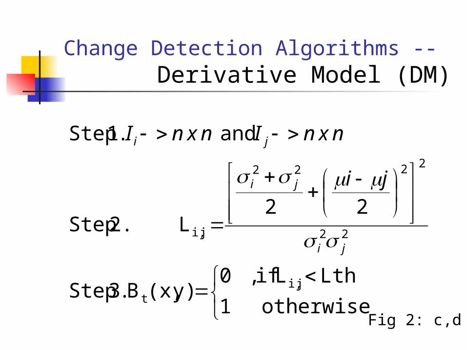
Change Detection Algorithms --Derivative Model (DM)

otherwise1

Lth L if,0y)(x,B .3 Step

22L 2. Step

and .1 Step

ji,t

22

2222

ji,ji

ji

ji

ji

nxnInxnI

Fig 2: c,d

Change Detection Algorithms --Shading Model (SM)

The intensity Ip at point (x,y)Ip= Ii * Sp , where Ii = illumination

Sp = shading coefficient

Calcuate the varance of the intensity Ip/Ip-1

0 => no changed Fig2 (e,f)

Change Detection Algorithms -- Local intensity gradient(LIG) method

Pixels at the location having a high gray-level gradient form a part of an object

Nearly pixles having similar gray levels will be also part of the same object.

Large negative gradients at pixels belonging to object boundaries

)}1,1(),(min{),( yxIyxIyxG

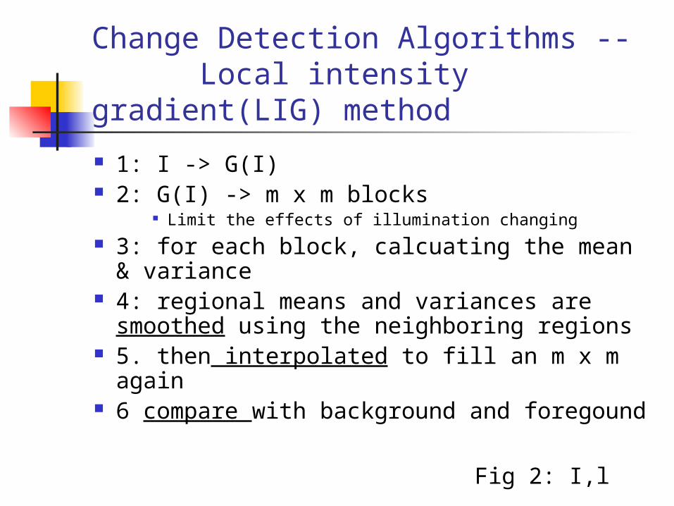
Change Detection Algorithms -- Local intensity gradient(LIG) method

1: I -> G(I) 2: G(I) -> m x m blocks

Limit the effects of illumination changing 3: for each block, calcuating the mean &

variance 4: regional means and variances are

smoothed using the neighboring regions 5. then interpolated to fill an m x m again 6 compare with background and foregound

Fig 2: I,l

Binary statistical morphology Mathematical morphology(MM) describe

images as sets and image-porcessing operators.

The main drawback of such operators is the high sensitivity to noise

Statistical morphology provides a noise-robust probabilistic generalization of MM.

Binary statistical morphology SM interprets erosion and dilation

as probabilistic lta and wta operator

Statistical erosion & statistical dilation = minimum variance estimators of the ouput distribution, P(H|I)

Binary statistical morphology SD computed at an image location

m as:

Binary Statistical Dilation(BSD) is obtained by threshold SD at value

)1)((

)(E

1

1

m

emMN

emM

B

B

)1,0(

1*

:j

HjBx

NmMmM

XmBcardmM

XmBcardmM

mM

mMNif

mM

mMNif

H

BB

cB

cB

B

B

B

B

m

)()(

)}{()(

)}{()(

)(

)()

1(ln0

)(

)()

1(ln1

01

0

1

1

1

1

1

*

)1()(

}2

1)(:{

],,0[,k xif 1][

}1)]([:{

1

1

i

1

e

NmM

NmMRi

RNxxV

mMVmBx

B

B

ii

Bi

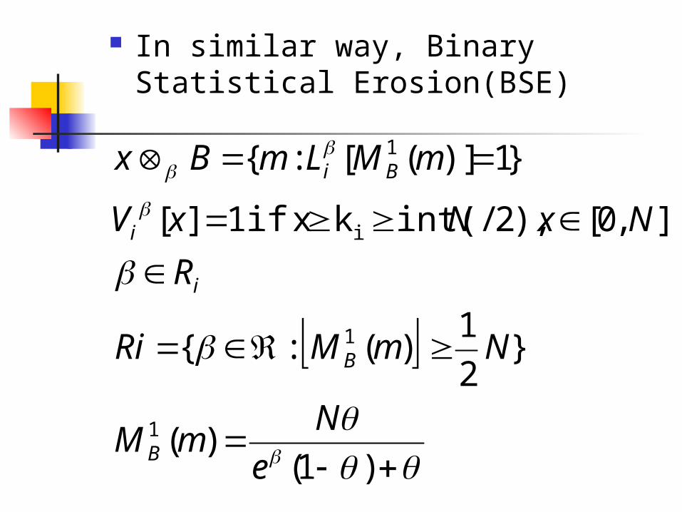
In similar way, Binary Statistical Erosion(BSE)

)1()(

}2

1)(:{

],,0[),2/int(k xif 1][

}1)]([:{

1

1

i

1

e

NmM

NmMRi

R

NxNxV

mMLmBx

B

B

i

i

Bi

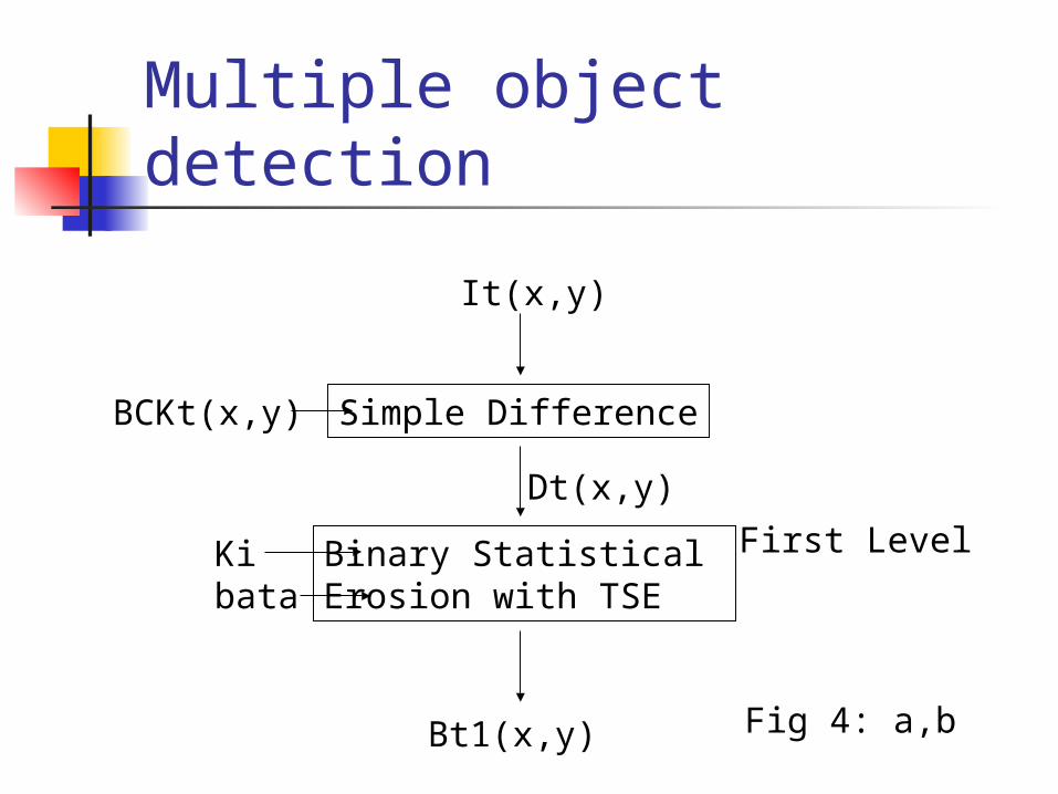
Multiple object detection

Simple Difference

It(x,y)

BCKt(x,y)

Dt(x,y)

Binary Statistical Erosion with TSE

Kibata

Bt1(x,y)

First Level

Fig 4: a,b

Multiple object detection -- The first step

Temporal structuring element (TSE) = 3x3 mask

A low ki value should be selected to maximize the probability of detecting moving object points.

The first level is represent the pixel where are object or background.

Multiple object detection -- The Second step (noise reduction)

Binary Statistical Erosion with TSE1

Bt1(x,y)

Set filtering

Binary Statistical dilation with TSE2

Zt(x,y)

Yt(x,y)

Bt2(x,y)

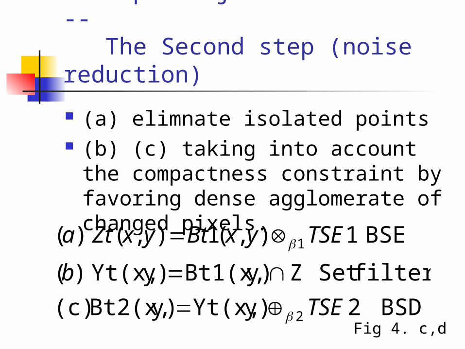
Multiple object detection -- The Second step (noise reduction)

(a) elimnate isolated points (b) (c) taking into account the

compactness constraint by favoring dense agglomerate of changed pixels.

BSD 2y)Yt(x,y)Bt2(x, (c)

filteringSet Zy)Bt1(x,y)Yt(x, )(

BSE 1),(1),( )(

2

1

TSE

b

TSEyxBtyxZta

Fig 4. c,d

Multiple object detection -- The Third step (blob tracking)

Blob tracking is a difficult task Many blobs may appear or vanish in

successive frames Blobs may be occluded by

overlapping of other blobs Problems are caused by the high

dimensionality of the set of possible combinations

See Fig 4. e

Multiple object detection -- The Third step (blob tracking)

Step1: a blob is not expected to be too far from where it was in the previous frame. Choose a mask,(2u*cosa+1 ) in x

direction and 2u*sina+1 in y direction The mask is centerred in I’s barycenter The blobs in I+1 frame whose

barycenter fall within this mask are selected.

Multiple object detection -- The Third step (blob tracking)

Step2:Let CBt+1(bi)= set of blobs on the

frame t+1 which are candidate to match with the blob bi detected on the frame t

=> 給定一 blob bi 選擇在下一個 frame,落在 bi 範圍內的 blob 集合

)](),(max[

| |

)(

2

1

biCBtu i

t uSuA

totaluuCF

面積附近的在下一個的面積

* 當 blob 大小不變時 ,cost function 值最小

A(v) )(

)](),(max[

|)()(|

CB(u)v

)(

2

1

uS

where

uSuA

uSuACF

i

biCBtu i

it

The cost function

Result-- The detection performance Tests on Outdoor Scenes

Fig 5. The detection performance

P=(correctly identified #) / (the method detected #)

即在此方法所有 detected 的 blob 中 , 有幾個是正確的 . R=(correct detected #)/ (original image #) G={(correctly identified #) -(false detected #)}/ (original image #)

Fig 7.

Result-- The Illumination conditions

Fig 8;

Result-- Overflow error & gap error

otherwise

iririf

where

iherrorGap

otherwise

iririf

where

igerrorOverflow

gr

H

i

gr

H

i

0

1)]()([1g(i)

)(k

1(Eo)

0

1)]()([1g(i)

)(k

1(Eo)

1

1

• r(i)=1, if i belong to the detected blob• rgr(i) =1, if i belong to the manually extracted blobs

Fig 9

Result-- Test on Noisy Images A random noise with uniform

distrubution was added to some frames of the image sequence.

Fig 10(a) SD and SM method could not be

applied to very noisy images. Fig 10(b) is proposed method result. Fig 11(a) is different noise level

result

Result-- Time performance The time performance of the

different CD methods were compared.

SD and proposed method are 10 times fast than the SM and DM

15 times faster than the LIG method

Conclusion If the system works outdoors and

in badly illuminated enviroments, => LIG , the proposed method If real-time is required, => the proposed method

Fig1: Original

Fig 2

SD method

DM method

Fig 2: SM result

Fig 2:LIG Result

Fig4:the proposed result

Fig5: more complex

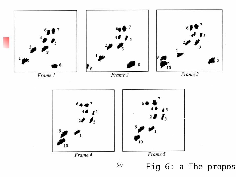
Fig 6: a The proposed

Fig6:b SD result

Fig 6: c SM result

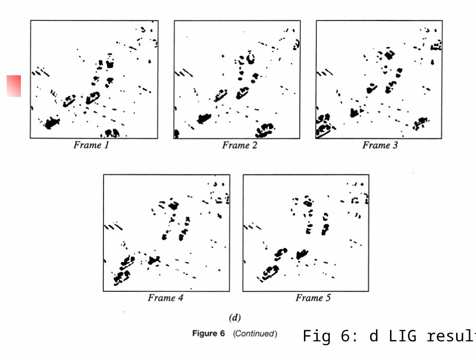
Fig 6: d LIG result

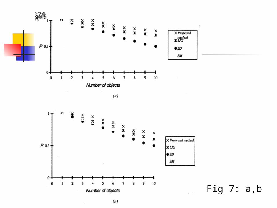
Fig 7: a,b

Fig 7: c

Fig 8: illum result

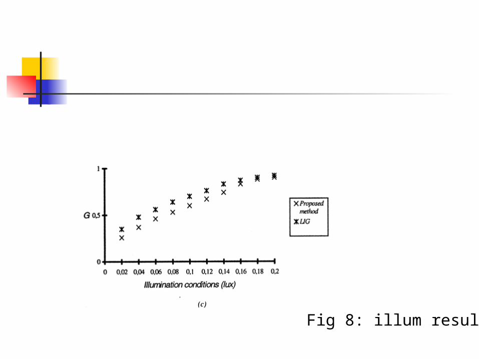
Fig 8: illum result

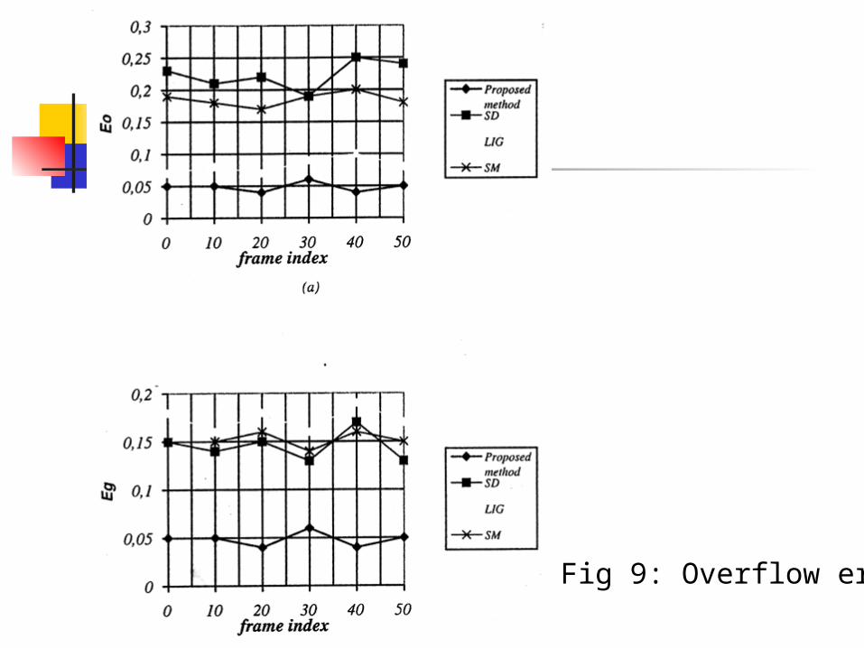
Fig 9: Overflow err

Fig 10 Noise