Real-Time Detection and Tracking of Vehicle Base Fronts ...cecas.clemson.edu/~stb/publications/vehicle_tracking_trb2007.pdf · In this paper we present an automatic technique for

Transportation Research Board Annual Meeting, Washington, D.C., January 2007. TRB Paper Number: 07-3308

Real-Time Detection and Tracking of Vehicle Base Fronts for Measuring Traffic Counts and

Speeds on Highways

Neeraj K. Kanhere Department of Electrical and Computer Engineering

207-A Riggs Hall Clemson University, Clemson, SC 29634

Phone: (864) 650-4844, FAX: (864) 656-5910 E-mail: [email protected]

Stanley T. Birchfield

Department of Electrical and Computer Engineering 207-A Riggs Hall

Clemson University, Clemson, SC 29634 Phone: (864) 656-5912, FAX: (864) 656-5910

E-mail: [email protected]

Wayne A. Sarasua Department of Civil Engineering

312 Lowry Hall, Box 340911 Clemson University, Clemson, SC 29634

Phone: (864) 656-3318, FAX: (864) 656-2670 E-mail: [email protected]

Tom C. Whitney

Department of Civil and Mechanical Engineering Technology South Carolina State University

300 College Street, Orangeburg, South Carolina 29117 E-mail: [email protected]

August 4, 2006

ABSTRACT We present a real-time system for automatically monitoring a highway when the camera is relatively low to the ground and on the side of the road. In such a case, occlusion and the perspective effects due to the heights of the vehicles cannot be ignored. The system presented in this paper is based on a novel technique of detecting and tracking base fronts of vehicles. Compared with our previous approach, the proposed technique involves a simplified problem formulation, operates in real time, and requires only a small number of parameters to calibrate. Experimental results of a camera mounted at a height of 26’ and a lateral distance of 12’ from the edge of pavement reveal accuracy as high as 98% with few false detections. The system can collect a variety of traffic data including volume, time-mean speed and space-mean speed, density, vehicle classification, and lane change activities. By handling perspective effects and vehicle occlusions, the system overcomes some of the limitations of commercially available machine vision-based traffic monitoring systems that are used in many intelligent transportation systems applications.

INTRODUCTION Traffic counts, speed and vehicle classification are fundamental data for a variety of transportation projects ranging from transportation planning to modern intelligent transportation systems (ITS). Most ITS applications are designed using readily available technology (e.g., sensors and communication), such as the inductive loop detector. Other sensing technologies include radar, infrared (IR), lasers, ultrasonic sensors and magnetometers. In (1) and (2), state of the art traffic sensing technologies are discussed along with the algorithms used to support traffic management functions.

Since the late 1980s, video detection systems have been marketed in the U.S. and elsewhere. Most popular video based traffic counting systems use high-angle cameras to count traffic by detecting vehicles passing digital sensors. As a pattern passes over the digital detector, the change is recognized and a vehicle is counted. The length of time that this change takes place can be translated into speed estimates. These systems use significant built-in heuristics to differentiate between shadows and vehicles in various weather conditions. The accuracy of such systems is compromised if the cameras are mounted too low or have poor perspective views of traffic. If the camera is not mounted high enough, the image of a vehicle “spill over” onto neighboring lanes, resulting in double counting.

A more promising approach to traffic monitoring is to track vehicles over time. This approach yields the trajectories of the vehicles, which are necessary for applications such as traffic flow modeling and counting turn movements. In this paper we present an automatic technique for detecting and tracking vehicle vehicle base fronts (VBFs) at a low angle, even in the presence of severe occlusion. There are significant benefits in terms of traffic data parameters that can be collected using vehicle tracking. Volume, time-mean speed, and vehicle classification are three common parameters that can be collected by most commercially based systems. Using tracking, space-mean speed through a long detection zone can be collected as well as time-mean speed. Space-mean speed gives a better estimate of traffic density than time-mean speed. Further, because of the longer detections zones, acceleration and deceleration characteristics can be collected, as well as specific lane-change maneuvers.

Kanhere, Birchfield, Sarasua, Whitney

Research in Vehicle Tracking Over the years researchers in computer vision have proposed various solutions to the automated tracking problem. These approaches can be classified as follows:

Blob Tracking. In this approach, a background model is generated for the scene. For each input image frame, the absolute difference between the input image and the background image is processed to extract foreground blobs corresponding to the vehicles on the road. Variations of this approach have been proposed in (3, 4, 5). Gupte et al. (3) perform vehicle tracking at two levels: the region level and the vehicle level, and they formulate the association problem between regions in consecutive frames as the problem of finding a maximally weighted graph. These algorithms have difficulty handling shadows, occlusions, and large vehicles (e.g., trucks, and trailers), all of which cause multiple vehicles to appear as a single region.

Active Contour Tracking. A closely related approach to blob tracking is based on tracking active contours (also known as snakes) representing the boundary of an object. Vehicle tracking using active contour models has been reported by Koller et al. (6), in which the contour is initialized using a background difference image and tracked using intensity and motion boundaries. Tracking is achieved using two Kalman filters, one for estimating the affine motion parameters (six parameters that account for scaling, shear, rotation and translation of an object in a plane), and the other for estimating the shape of the contour. An explicit occlusion detection step is performed by intersecting the depth ordered regions associated with the objects. The intersection is excluded in the shape and motion estimation. As with the previous technique, results are shown on image sequences without shadows or severe occlusions, and the algorithm is limited to tracking cars.

3D-Model Based Tracking. Tracking vehicles using three-dimensional models has been studied by several research groups (7, 8, 9, 10). Some of these approaches assume an aerial view of the scene which virtually eliminates all occlusions (10) and match the three-dimensional wireframe models for different types of vehicles to edges detected in the image. In (9), a single vehicle is successfully tracked through a partial occlusion, but its applicability to congested traffic scenes has not been demonstrated.

Markov Random Field Tracking. An algorithm for segmenting and tracking vehicles in low-angle frontal sequences has been proposed by Kamijo et al. (11). In their work, the image is divided into pixel blocks, and a spatiotemporal Markov random field (ST-MRF) is used to update an object map using the current and previous image. One drawback of the algorithm is that it does not yield 3D information about vehicle trajectories in the world coordinate system. In addition, in order to achieve accurate results the images in the sequence are processed in reverse order to ensure that vehicles recede from the camera. The accuracy decreases by a factor of two when the sequence is not processed in reverse, thus making the algorithm unsuitable for on-line processing when time-critical results are required.

Feature Tracking. In this approach, instead of tracking a whole object, feature points on an object are tracked. The method is useful in situations of partial occlusions, where only a portion of an object is visible. The task of tracking multiple objects then becomes the task of grouping the tracked features based on one or more similarity criteria. Beymer et al. (12,13) have proposed a feature tracking based approach for traffic monitoring applications. In their approach, point features are tracked throughout the detection zone specified in the image. Feature points which are tracked successfully from the entry region to the exit region are considered in the process of

3


grouping. Grouping is done by constructing a graph over time, with vertices representing sub-feature tracks and edges representing the grouping relationships between tracks. The algorithm was implemented on multi-processor digital signal processing (DSP) board for real-time performance. Results were reported for day and night sequences with varying levels of traffic congestion. For proper grouping, the features need to be tracked over the entire detection zone which is often not possible (when the camera is not looking top-down) due to significant scale changes and occlusions. In (14) Saunier et al. use feature points for tracking vehicles at intersections where they address the problem of features not being tracked throughout the processing region.

Color and Pattern-Based Tracking. Chachich et al. (15) use color signatures in quantized RGB space for tracking vehicles. In this work, vehicle detections are associated with each other by combining color information with driver behavior characteristics and arrival likelihood. In addition to tracking vehicles from a stationary camera, a pattern-recognition based approach to on-road vehicle detection has been studied in (16). The camera is placed inside a vehicle looking straight ahead, and vehicle detection is treated as a pattern classification problem using support vector machines (SVMs).

APPROACH As mentioned in our previous approach (17, 18), a single homography (plane-to-plane mapping) is often insufficient to correctly segment all the foreground pixels in an image because of the depth ambiguity in the scene observed from a single camera. The depth ambiguity arises from the fact that for a point in the world, every point lying on the ray passing through the camera-centre and that point are projected as a single point in an image. Unlike our previous approach where we segment all of the feature points into groups (representing vehicles) by estimating their world coordinates to account for effect of heights of vehicles, in our current approach we detect regions in the image where the depth ambiguity is absent. Since the base of a vehicle is in direct contact with the road, there is no ambiguity in mapping it from the image coordinates to the world coordinates using a single homography.

The key part of this new approach is the detection and tracking of the front side of a vehicle’s base, which we refer to as a vehicle base front (VBF). Often two or more vehicles appear as a single blob in the foreground mask as a result of partial occlusions and a non-ideal perspective view of the scene. In such situations detecting VBFs helps in separating and tracking individual vehicles. In order to improve the accuracy of tracking, feature points associated with a VBF are tracked. When an image frame lacks sufficient evidence to track a VBF by matching, feature points associated with a VBF are used to predict and update its location in consecutive frames.

Calibration Process To account for scale changes due to perspective effects and to successfully detect VBFs, a calibration step is necessary. The calibration process is much more simplified from our previous approach. A user needs to specify only four points on the road, along with the width, length and the number of lanes in the detection zone formed by these points as illustrated in Figure 1. For counting vehicles, an approximate width to length ratio is sufficient, but accurate speed measurement requires an accurate ratio.

4


The homography is defined by a 3x3 matrix H having eight parameters (Since overall scale is not important, the last element of the matrix is set to a fixed value of 1). Each calibration point leads to two equations, so that four such non-collinear points are needed for an exact solution to the eight unknown elements in H. Throughout this paper, the mapping between image coordinates and the road-plane coordinates will be denoted as

P’ = H P and P = H -1P’,

where P and P’ are homogeneous coordinates in the image plane and road plane, respectively, of a world point.

FIGURE 1 Calibration process.

(a) (b)

(a) Calibration tool. (b) Top-view of the detection zone.

Background Subtraction

Background subtraction is a simple and effective technique for extracting foreground objects from a scene. The process of background subtraction involves initializing and maintaining a background model of the scene. At run time, the estimated background image is subtracted from the input frame, followed by thresholding the difference image and morphological processing to reduce the effects of noise, in order to yield foreground blobs. A review of several background modeling techniques is presented in (19) where the authors claim adaptive median filtering to be a good balance between computational cost and quality of the results. At run time, only the pixels that are not labeled as foreground pixels are used to update the background, the step size being used to control the rate at which this update occurs. For the scope of this research, adaptive median filtering was used, although preliminary experimentation indicated that averaging and standard median filtering produce similar results. Moving shadows

5


are a major problem for successful detection and tracking of vehicles in most tracking algorithms. A summary of different techniques for detecting moving shadows in grayscale and color images is presented in (20, 21).

FIGURE 2 Background subtraction and shadow detection.

(a) (b)

(c) (d)

(a) Input frame. Pixels in hatched region are monitored for shadows. (b) Computed background image. (c) Foreground mask without shadow detection. (d) Foreground mask

with shadows detected and removed.

We implemented a basic shadow-detection module where the difference image D is

computed as: D (x, y) = 0 if NTL < B(x, y) – I(x, y) < NTH = | I(x, y) – B(x, y) | otherwise

where I is the input frame, B is the background image, and the shadow thresholds (NTL, NTH) are user-defined.

The thresholds were decided empirically by observing the intensities corresponding to a manually-selected shadow region. Figure 2 (a) shows this region (the cross-hatched rectangle) and Figure 2 (b) shows the background image for the sequence. Figure 2 (c) and (d) illustrate the

6


result of applying the shadow detection step. Notice that dark pickup truck (in the lane closest to the shoulder) which is overshadowed by the large truck adjacent to it is detected after removing the shadows. The requirement of setting the shadow thresholds manually could be replaced by an extension to the current implementation in which a region outside the detection zone (similar to the cross-hatched rectangle in the figure) would be monitored for the presence of shadows, and the thresholds would be chosen automatically from the intensity differences observed over time in that region.

Detection of Vehicle Base Fronts For each input frame as shown in Figure 3 (a), background subtraction is followed by morphological operations (dilation and erosion) to yield foreground blobs, shown in Figure 3 (b). Pixels corresponding to the base of a vehicle are easily found using a difference operator in the vertical direction:

B(x, y) = 1 if F(x, y) – F(x, y+1) > 0

= 0 otherwise

where the foreground pixels are labeled with a positive value, while the background pixels are labeled with the value of zero. The resulting base image B is shown in Figure 3 (c).

After projecting the base image on the road plane using the homography matrix H, connected component analysis is performed to select only the front side of a base region (i.e., the segment oriented in the horizontal direction). The reason for selecting only the front of a base is that the sides of a base are more likely to be occluded due to shadows and adjacent vehicles, whereas the fronts of vehicle bases appear disjoint even under partial occlusions. Base fronts are tracked in the projected plane to reduce the sensitivity of tracking parameters to scale changes. It should be noted that, although region- and contour-based approaches can handle occlusions if the vehicles enter the scene un-occluded, such techniques fail when the camera angle is low because multiple vehicles often enter the scene partially occluded.

The ability of VBFs to separate vehicles which appear as a single blob in a cluttered scene is illustrated in Figure 3. This is where our current approach differs from previous approaches, including our earlier work (17, 18). Instead of segmenting all the foreground pixels (or feature points) in the presence of depth ambiguity, we select and segment only those pixels for which there is no depth ambiguity (i.e., a vehicle base front). For counting vehicles and measuring speeds, tracking VBFs yields accurate results since vehicles are segmented at the beginning of the detection zone even when partially occluded.

Base-Constrained Regions Occasionally while tracking a VBF, a corresponding match cannot be found in the next frame, for instance a vehicle being tracked moves very close to a vehicle traveling ahead of it, which causes the VBF of the tracked vehicle to be occluded. In such a scenario, feature points associated with that VBF are used to predict its location. These features are selected from a region in the image to which we refer as a base-constrained region. Any feature point found in this region is likely to lie on the vehicle associated with that VBF under the assumed box model.

7


FIGURE 3 Detection of Vehicles in Clutter Using Vehicle Base Fronts.

(a) (b) (c) (d)

(e) (f)

(g) (h)

(a) Input frame. (b) Foreground mask. (c) Base pixels. (d) Base pixels mapped into the top-view using homography. (e) Input frame. (f) Foreground mask. Multiple vehicles appear as a single blob. (g) and (h) Detected vehicle base fronts in image and top-view.

Note that partially occluding vehicles are initialized separately.

8


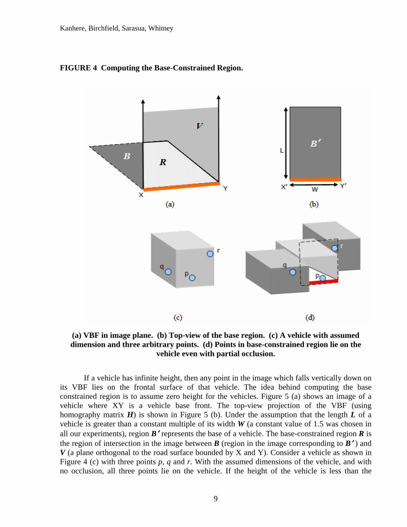
FIGURE 4 Computing the Base-Constrained Region.

(a) VBF in image plane. (b) Top-view of the base region. (c) A vehicle with assumed dimension and three arbitrary points. (d) Points in base-constrained region lie on the

vehicle even with partial occlusion.

If a vehicle has infinite height, then any point in the image which falls vertically down on its VBF lies on the frontal surface of that vehicle. The idea behind computing the base constrained region is to assume zero height for the vehicles. Figure 5 (a) shows an image of a vehicle where XY is a vehicle base front. The top-view projection of the VBF (using homography matrix H) is shown in Figure 5 (b). Under the assumption that the length L of a vehicle is greater than a constant multiple of its width W (a constant value of 1.5 was chosen in all our experiments), region B’ represents the base of a vehicle. The base-constrained region R is the region of intersection in the image between B (region in the image corresponding to B’ ) and V (a plane orthogonal to the road surface bounded by X and Y). Consider a vehicle as shown in Figure 4 (c) with three points p, q and r. With the assumed dimensions of the vehicle, and with no occlusion, all three points lie on the vehicle. If the height of the vehicle is less than the

9


assumed height as shown in Figure 4 (d), the point r will no longer be on the vehicle. Similarly the point q is now on the occluding vehicle whereas the point p which lies in the base-constrained region (shown in white) is still on the same vehicle.

Tracking Features For each VBF, feature points are automatically selected in the corresponding base-constrained region and tracked using the Kanade-Lucas-Tomasi (KLT) feature tracker (22) based on the algorithm proposed in (23) which computes the displacement d that minimizes the sum of squared differences between consecutive image frames I and J.

where W is a window of pixels around the feature point. The nonlinear error is minimized by repeatedly solving its linearized version:

where,

As in (23), features are automatically selected as those points in the image for which both eigenvalues of Z are greater than a minimum threshold. During tracking, if a match is found for a VBF in the next frame, the list of features associated with it is updated. In case the match is not found, the location of the VBF in the next frame is predicted using the mean displacement of the features associated with it.

Tracking Vehicle Base Fronts Tracking is achieved by matching detections in the new frame with the existing VBFs. The steps in the tracking algorithm are as follows:

1) The background image is subtracted from the input frame and after suppressing shadows, hysteresis thresholding and morphological operations are performed to compute foreground mask.

2) Vehicle base fronts are detected in the image as described in the previous section, and the top-view of VBFs is computed using homography matrix H. Filtering is performed to discard VBFs having width less than a Wmin (which is computed as a multiple of lane-width and kept constant for processing all the sequences).

10


3) Each existing VBF is matched with the detected VBFs in the current frame using nearest neighbor search. The distance between an existing vehicle base front A and a new detection B is computed as

d (A, B) = min { E(AL,BL), E(AR,BR) } where E(A, B) is the Euclidean distance between two points A and B. Subscripts L and R indicate left and right end points of a VBF in the projected top-view. The best match i corresponds to the detection Bi that is closest to the VBF being tracked. The search for the nearest neighbor is limited to a distance DN proportional to the lane width.

4) If a close match is found as described in step 3, the location of the VBF is updated, and features that lie in the corresponding base-constrained region are associated with it.

5) If a close match is not found in step 3, the VBF is labeled as missing and its displacement in the next frame is estimated as the mean displacement of the features associated with it.

6) Each missing VBF is matched with the detected VBFs (in the current frame) that are not already associated with another VBF. If a match is found, the missing VBF is re-initialized with the matched VBF.

7) Each detected VBF that is not associated with another VBF is initialized as a new vehicle detection if its width is greater than a threshold (Wnew), which is computes in terms of lane-width.

8) A missing VBF is marked invalid and is not processed further if the number of frames for which it is missing is more than the number of frames for which it was tracked.

9) When a VBF (tracked or missing) exits the detection zone, corresponding measurements such as lane counts and speeds are updated using its trajectory.

Classification The type of the vehicle (truck or car) is determined (in the frame in which the vehicle exits the detection zone) by measuring the height (from the centre of VBF) and length (from an endpoint of a VBF) of a blob. A vehicle is classified as a truck when both the length and the height of the blob are greater than corresponding thresholds. If a vehicle is traveling on the far side of an occluding vehicle, then the length of the corresponding blob will be more than the length- threshold (CTL), but the height of the blob from the centre of VBF will be less than the height-threshold (CTH), and the vehicle will not be misclassified as a truck. On the other hand, if a vehicle is traveling on the near side of another vehicle, then the height of the blob will be more than the height threshold, but the length will be less than a threshold, which will prevent the vehicle from being misclassified as a truck. The threshold values are computed in terms of the lane-width.

EXPERIMENTAL RESULTS The proposed algorithm was implemented in the C++ language to develop a real-time system for counting vehicles (lane counts) on freeways and single- and multi-lane highways, measuring speeds, and classifying detected vehicles (car and truck). The system uses the Blepo Computer Vision Library being developed at Clemson University (24).

11


To compare the accuracy of the proposed system it was tested on four different sequences with varying traffic and weather conditions. The camera was mounted on a 26’ tripod approximately 12’ from the side of the road and the sequences were digitized at 320 x 240 resolution and 30 frames per second. No preprocessing was done to stabilize occasional camera jitter or to compensate for lighting conditions. For each sequence, offline camera calibration was performed once, as explained earlier.

The first sequence was captured on a clear day. The sample frame is shown in Figure 5- (a). Vehicles are traveling in three lanes and there are strong moving shadows with service level C traffic. The second sequence, as shown in Figure 5 (j), has a four-lane highway with the last lane blocked for maintenance work. The lane closure results in slow moving traffic with vehicles traveling close to each other. The sequence was captured during data collection for studying the effect of a workzone on freeway traffic (25). The third sequence was found to be more challenging because the vehicles cast long shadows. The fourth sequence, shown in Figure 5 (m) was also captured for the workzone study with service level A traffic. Vehicles are traveling close to each other at low speeds. Because of the presence of fog, the images in this sequence are noisy compared with those in the other sequences. Experiments were carried out using 1) no shadow suppression and no feature points, 2) using shadow detection but no KLT feature points and 3) using shadow detection and using KLT feature points. In the absence of KLT feature points, the displacement of a missing VBF is estimated from its displacement in the previous frames.

Figure 5 shows some of the output frames from the test sequences. In Figure 5(a) and (c), the system successfully detects and tracks the white car in the middle lane which is partially occluded by a small truck in the first lane (lane closest to the camera). The white car is correctly counted even after it is completely occluded by the truck when it exits the detection zone. In Figure 5(d) to (f) vehicles are traveling close to each other and appear as a single blob throughout the detection zone. Except for the distant car in the middle lane, all the other vehicles are successfully tracked and counted by the system.

In Figure 5(g) to (i) the system detects the vehicle in the middle lane at the beginning of the detection zone. When the VBF of that vehicle is occluded behind the car traveling in the first lane Figure 5(h), feature points are used to predict its location in the following frames and finally the vehicle is recovered in Figure 5(i) when it is changing lanes. In Figure 5(j) to (l) the ability of the system to detect and track vehicles under partial occlusion is demonstrated. In Figure 5(o) the vehicle in the second lane passes undetected because its VBF is occluded by a pickup truck traveling in the adjacent (first) lane.

Quantitative analysis of the system’s performance is shown in Table 1. The detection rate is above 90% in all the sequences. In sequences 2 and 3, false detections are caused by shadows (although shadow suppression reduced the number of false positives, but did not eliminate the problem completely) and occasional splitting of the foreground mask (when brightness of a vehicle matches closely with that of road). Using KLT features improves the results because in case a direct match is not found for a VBF, mean feature point displacement gives more accurate predication of its location compared to the prediction computed from just the previous displacement.

12


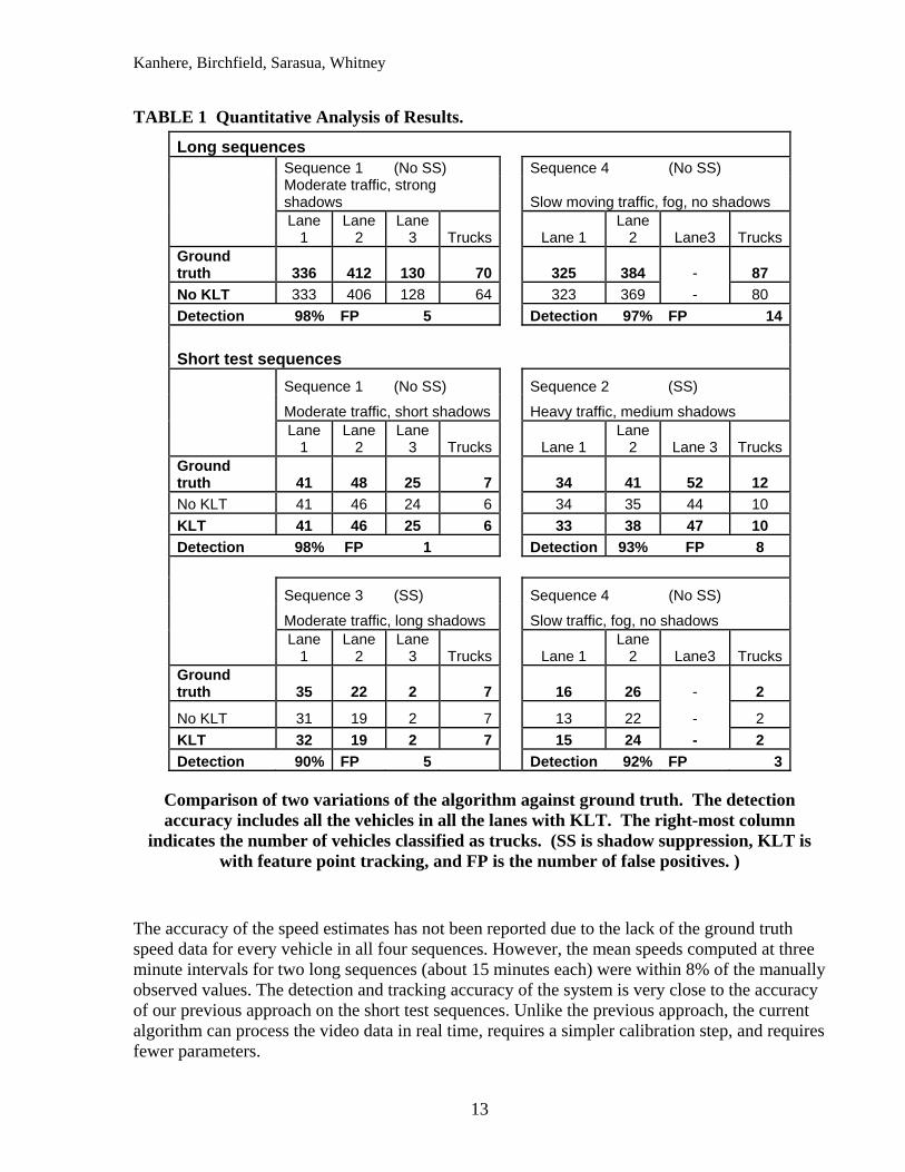
TABLE 1 Quantitative Analysis of Results.

Long sequences Sequence 1 (No SS) Sequence 4 (No SS)

Moderate traffic, strong shadows Slow moving traffic, fog, no shadows

Lane

1 Lane

2 Lane

3 Trucks Lane 1 Lane

2 Lane3 TrucksGround truth 336 412 130 70 325 384 - 87 No KLT 333 406 128 64 323 369 - 80 Detection 98% FP 5 Detection 97% FP 14 Short test sequences

Sequence 1 (No SS) Sequence 2 (SS)

Moderate traffic, short shadows Heavy traffic, medium shadows

Lane

1 Lane

2 Lane


2 Lane 3 TrucksGround truth 41 48 25 7 34 41 52 12 No KLT 41 46 24 6 34 35 44 10 KLT 41 46 25 6 33 38 47 10 Detection 98% FP 1 Detection 93% FP 8

Sequence 3 (SS) Sequence 4 (No SS)

Moderate traffic, long shadows Slow traffic, fog, no shadows

Lane

1 Lane

2 Lane


2 Lane3 TrucksGround truth 35 22 2 7 16 26 - 2

No KLT 31 19 2 7 13 22 - 2 KLT 32 19 2 7 15 24 - 2 Detection 90% FP 5 Detection 92% FP 3

Comparison of two variations of the algorithm against ground truth. The detection accuracy includes all the vehicles in all the lanes with KLT. The right-most column

indicates the number of vehicles classified as trucks. (SS is shadow suppression, KLT is with feature point tracking, and FP is the number of false positives. )

The accuracy of the speed estimates has not been reported due to the lack of the ground truth speed data for every vehicle in all four sequences. However, the mean speeds computed at three minute intervals for two long sequences (about 15 minutes each) were within 8% of the manually observed values. The detection and tracking accuracy of the system is very close to the accuracy of our previous approach on the short test sequences. Unlike the previous approach, the current algorithm can process the video data in real time, requires a simpler calibration step, and requires fewer parameters.

13


FIGURE 5 Experimental Results.

(a) (b) (c)

(d) (e) (f)

(g) (h) (i)

(j) (k) (l)

(m) (n) (o)

14


A sequence (short sequence-1) was analyzed using a commercial system. The detection markers were placed (by an experienced user of the system) to maximize the vehicle count accuracy. The same sequence was tested using the proposed system and it was found that out of the 114 vehicles the commercial system detected 108 vehicles with 8 false positives (double counts) whereas the proposed system detected 112 vehicles with just 1 false detection. The same parameter values were used for all the sequences (CTL=1.0, CTL = 0.5, DN = 2.0, Wmin = 0.5, Wnew = 0.7). With the value used for Wnew the system is unable to detect motorcycles. Using a smaller value for Wnew it is possible to detect motorcycles but leads to increased false positives. Shadow detection was used for Sequence 2 and 3 to reduce false positives (NTL = 30, NTH = 50). The average processing speed was found to be 34 frames per second which demonstrate the ability of the system to operate in real time.

CONCLUSIONS AND RECOMMENDATIONS Most approaches to segmenting and tracking vehicles from a stationary camera assume that the camera is high above the ground, thus simplifying the problem. A technique has been presented in this paper that works when the camera is at a relatively low angle with respect to the ground and/or is on the side of the road, in which case occlusions are more frequent. A real-time system was implemented and tested based on the proposed algorithm. The results demonstrate the ability of the proposed system to correctly track and count vehicles on freeways even in cases where multiple vehicles simultaneously enter the detection zone partially occluded. The system can collect a variety of traffic data including volume, time-mean speed and space-mean speed, density, vehicle classification, and lane change activities.

Some of the aspects of the proposed system need further analysis and improvement. A simple approach has been adopted for the classification of the tracked vehicles which is prone to errors when vehicles are traveling very close to each other. Combining color and motion information will help to make the tracker more robust. We envision using VBFs for initialization of occluded vehicles, counts, and speed measurements, while using a more detailed model (based on additional attributes) to track vehicles over multiple cameras with or without overlapping views. In addition, future research should be aimed at handling low-angle image sequences taken at intersections, where the resulting vehicle trajectories are more complicated than those on highways.

ACKNOWLEDGMENT We would like to thank the James Clyburn Transportation Center at South Carolina State University and the Dwight David Eisenhower Transportation Fellowship Program for funding this research.

References 1. Lawrence A. Klein, Sensor Technologies and Data Requirements for ITS, Boston: Artech

House, 2001. 2. Dan Middleton, Deepak Gopalakrishna, and Mala Raman. Advances in traffic data

collection and management (white paper), January 2003. http://www.itsdocs.fhwa.dot.gov/JPODOCS/REPTS_TE/13766.html (Accessed on June 23, 2005)

15


3. S. Gupte, O. Masoud, R. F. K. Martin, and N. P. Papanikolopoulos. Detection and

classification of vehicles. IEEE Transactions on Intelligent Transportation Systems, 3(1):37–47, March 2002.

4. D. Magee. Tracking multiple vehicles using foreground, background and motion models.

In Proceedings of ECCV Workshop on Statistical Methods in Video Processing, (2002).

5. D. Daily, F.W. Cathy, and S. Pumrin. An algorithm to estimate mean traffic speed using uncalibrated cameras. In IEEE Conference for Intelligent Transportation Systems, pages 98–107, 2000.

6. D. Koller, J. Weber, and J. Malik. Robust multiple car tracking with occlusion reasoning.

In European Conference on Computer Vision, pages 189–196, 1994.

7. D. Koller, K Dandilis, and H. H. Nagel. Model based object tracking in monocular image sequences of road traffic scenes. International Journal of Computer Vision, 10(3):257–281, 1993.

8. M. Haag and H. Nagel. Combination of edge element and optical flow estimate for 3D-

model-based vehicle tracking in traffic image sequences. International Journal of Computer Vision, 35(3):295–319, Dec 1999.

9. J. M. Ferryman, A. D. Worrall, and S. J. Maybank. Learning enhanced 3d models for

vehicle tracking. In British Machine Vision Conference, pages 873–882, 1998.

10. C. Schlosser, J. Reitberger, and S. Hinz. Automatic car detection in high resolution urban scenes based on an adaptive 3D-model. In EEE/ISPRS Joint Workshop on Remote Sensing and Data Fusion over Urban Areas, Berlin, pages 98–107, 2003.

11. S. Kamijo, K. Ikeuchi, and M. Sakauchi. Vehicle tracking in low-angle and front view

images based on spatio-temporal markov random fields. In Proceedings of the 8th World Congress on Intelligent Transportation Systems (ITS), 2001.

12. D. Beymer, P. McLauchlan, B. Coifman, and J. Malik. A real time computer vision

system for measuring traffic parameters. In IEEE Conference on Computer Vision and Pattern Recognition, pages 495–501, 1997.

13. Jitendra Malik and Stuart Russel. Final Report for Traffic Surveillance and Detection

Technology Development New Traffic Sensor Technology, December 19, 1996. http://citeseer.ist.psu.edu/malik96final.html (Accessed on October 21, 2005).

14. Saunier N. and Sayed T. A Feature-Based Tracking Algorithm for Vehicles in

Intersections. Third Canadian Conference on Computer and Robot Vision, June 2006.

16


15. Chachich, A. A. Pau, A. Barber, K. Kennedy, E. Oleiniczak, J. Hackney, Q. Sun, E. Mireles, "Traffic sensor using a color vision method," Proceedings of the International Society for Optical Engineering, Vol. 2902, pp. 156-164, January 1997.

16. Zehang Sun, George Bebis and Ronald Miller. Improving the Performance of On-Road

Vehicle Detection by Combining Gabor and Wavelet Features. In Proceedings of the 2002 IEEE International Conference on Intelligent Transportation Systems, September 2002.

17. Neeraj K. Kanhere, Shrinivas J. Pundlik, and Stanley T. Birchfield. Vehicle segmentation

and tracking from a low-angle off-axis camera. In IEEE Conference on Computer Vision and Pattern Recognition, pages 1152–1157, 2005.

18. Neeraj K. Kanhere, Stanley T. Birchfield, and Wayne A. Sarasua. Vehicle Segmentation

and Tracking in the Presence of Occlusions. Transportation Research Record, ,Transportation Research Board, in press .

19. S. C. Cheung and Chandrika Kamath. Robust techniques for background subtraction in

urban traffic video. In Proceedings of Electronic Imaging: Visual Communications and Image Processing, 2004.

20. Andrea Prati, Ivana Mikic, Moahan M. Trivedi and Rita Cucchiara. Detecting Moving

Shadows: Algorithms and evaluation. In IEEE Transactions on Pattern Analysis and Machine Intelligence, Vol. 25 (7), pp. 918-923, 2003.

21. P. Rosin and T. Ellis. Image difference threshold strategies and shadow detection. In

Proceedings of the 6th British Machine Vision Conference, pp. 347-356, BMVA press, 1995.

22. S. Birchfield. KLT: An implementation of the Kanade-Lucas-Tomasi feature tracker.

http://www.ces.clemson.edu/~stb/klt/ (Accessed on June 17, 2006)

23. Carlo Tomasi and Takeo Kanade. Detection and tracking of point features. Technical Report CMU-CS-91-132, Carnegie Mellon University, Apr 1991.

24. Blepo Computer Vision Library: An open-source C/C++ library to facilitate computer

vision research and education. http://www.ces.clemson.edu/~stb/blepo/ (Accessed on July 30, 2006)

25. Wayne Sarasua. Traffic Impacts of Short Term Interstate Work Zone Lane Closures: The South Carolina Experience. http://ops.fhwa.dot.gov/wz/workshops/accessible/Sarasua.htm (Accessed on July 21, 2006)

17

http://www.ces.clemson.edu/%7Estb/publications/vehicle_tracking_trb2006.pdf

http://www.ces.clemson.edu/%7Estb/publications/vehicle_tracking_trb2006.pdf

http://www.ces.clemson.edu/~stb/blepo/

Documents

Real-Time Detection and Tracking of Vehicle Base Fronts ...cecas.clemson.edu/~stb/publications/vehicle_tracking_trb2007.pdf · In this paper we present an automatic technique for