Embed Size (px)
Citation preview

Real-time Control and Optimization
of Water Supply & Distribution
Infrastructure
by
Thouheed Abdul Gaffoor
A thesis
presented to the University of Waterloo
in fulfillment of the
thesis requirement for the degree of
Master of Applied Science
in
Civil Engineering
Waterloo, Ontario, Canada, 2017
c© Thouheed Abdul Gaffoor 2017

I hereby declare that I am the sole author of this thesis. This is a true copy of the thesis,
including any required final revisions, as accepted by my examiners.
I understand that my thesis may be made electronically available to the public.
ii

Abstract
Across North America, water supply and distribution systems (WSDs) are controlled
manually by operational staff - who place a heavy reliance on their experience and judge-
ment when rendering operational decisions. These decisions range from scheduling the
operation of pumps, valves and chemical dosing in the system. However, due to the
uncertainty of demand, stringent water quality regulatory constraints, external forcing
(cold/drought climates, fires, bursts) from the environment, and the non-stationarity of
climate change, operators have the tendency to control their systems conservatively and
reactively. WSDs that are operated in such fashion are said to be ’reactive’ because: (i)
the operators manually react to changes in the system behaviour, as measured by Super-
visory Control and Data Acquisition (SCADA) systems; and (ii) are not always aware of
any anomalies in the system until they are reported by consumers and authorities. The
net result is that the overall operations of WSDs are suboptimal with respect to energy
consumption, water losses, infrastructure damage and water quality.
In this research, an intelligent platform, namely the Real-time Dynamically Dimen-
sioned Scheduler (RT-DDS), is developed and quantitatively assessed for the proactive
control and optimization of WSD operations. The RT-DDS platform was configured to
solve a dynamic control problem at every timestep (hour) of the day. The control prob-
lem involved the minimization of energy costs (over the 24-hour period) by recommending
’near-optimal’ pump schedules, while satisfying hydraulic reliability constraints. These
constraints were predefined by operational staff and regulatory limits and define a toler-
ance band for pressure and storage levels across the WSD system. The RT-DDS platform
includes three essential modules. The first module produces high-resolution forecasts of
water demand via ensemble machine learning techniques. A water demand profile for the
iii

next 24-hours is predicted based on historical demand, ambient conditions (i.e. temper-
ature, precipitation) and current calendar information. The predicted profile is then fed
into the second module, which involves a simulation model of the WSD. The model is used
to determine the hydraulic impacts of particular control settings. The results of the simu-
lation model are used to guide the search strategy of the final module - a stochastic single
solution optimization algorithm. The optimizer is parallelized for computational efficiency,
such that the reporting frequency of the platform is within 15 minutes of execution time.
The fidelity of the prediction engine of the RT-DDS platform was evaluated with an
Advanced Metering Infrastructure (AMI) driven case study, whereby the short-term water
consumption of the residential units in the city were predicted. A Multi-Layer Perceptron
(MLP) model alongside ensemble-driven learning techniques (Random forests, Bagging
trees and Boosted trees) were built, trained and validated as part of this research. A three-
stage validation process was adopted to assess the replicative, predictive and structural
validity of the models. Further, the models were assessed in their predictive capacity
at two different spatial resolutions: at a single meter and at the city-level. While the
models proved to have strong generalization capability, via good performance in the cross-
validation testing, the models displayed slight biases when aiming to predict extreme peak
events in the single meter dataset. It was concluded that the models performed far better
with a lower spatial resolution (at the city or district level) whereby peak events are far
more normalized. In general, the models demonstrated the capacity of using machine
learning techniques in the context of short term water demand forecasting - particularly
for real-time control and optimization.
In determining the optimal representation of pump schedules for real-time optimization,
multiple control variable formulations were assessed. These included binary control statuses
and time-controlled triggers, whereby the pump schedule was represented as a sequence of
iv

on/off binary variables and active/idle discrete time periods, respectively. While the time
controlled trigger representation systematically outperformed the binary representation in
terms of computational efficiency, it was found that both formulations led to conditions
whereby the system would violate the predefined maximum number of pump switches per
calendar day. This occurred because at each timestep the control variable formulation was
unaware of the previously elapsed pump switches in the subsequent hours. Violations in the
maximum pump switch limits lead to transient instabilities and thus create hydraulically
undesirable conditions. As such, a novel feedback architecture was proposed, such that
at every timestep, the number of switches that had elapsed in the previous hours was
explicitly encoded into the formulation. In this manner, the maximum number of switches
per calendar day was never violated since the optimizer was aware of the current trajectory
of the system. Using this novel formulation, daily energy cost savings of up to 25% were
achievable on an average day, leading to cost savings of over 2.3 million dollars over a ten-
year period. Moreover, stable hydraulic conditions were produced in the system, thereby
changing very little when compared to baseline operations in terms of quality of service
and overall condition of assets.
v

Acknowledgements
I would like to take this opportunity to sincerely express my gratitude to Dr. Bryan Tol-
son, my M.A.Sc. supervisor, for his continuous guidance and support throughout both my
undergraduate and graduate studies at Waterloo. Bryan not only diligently and patiently
advised me, but enthusiastically mentored me throughout my years at the University of
Waterloo. The intellectually stimulating comments and thoughts he has shared with me
have always motivated me to advance my own research and interests in entrepreneurship.
Through his mentorship and friendship, I’ve learnt a great deal and am truly grateful.
There are also a number of individuals from the Department of Civil and Environmental
Engineering whom I’d like to acknowledge: most notably Amin Jahanpour, Dr. David
Brush and Dr. Monica Emelko for their incalculable influence on my intellectual and ca-
reer development; as well as Dr. Donald Burn and Dr.Liping Fu for taking the time and
effort to review my Thesis.
I would also like to thank my family - specifically my parents and my fiancee, Mariam,
whom I am entirely indebted to. Without their support, constant encouragement and
sacrifices, none of this would’ve been possible. I am also grateful to my brothers, who
painfully endured my whining throughout my graduate (and sadly undergraduate) career.
This research was funded by my Graduate Research Scholarship (GRS), and supported
by the Natural Science & Engineering Research Council (NSERC), our industry partners
C3Water and the City of Guelph.
vi

Table of Contents
List of Tables xi
List of Figures xii
1 Introduction 1
1.1 Motivation . . . . . . . . . . . . . . . . . . . . . . . . . . . . . . . . . . . . 2
1.2 Proposed Solution . . . . . . . . . . . . . . . . . . . . . . . . . . . . . . . . 4
1.3 Related Research . . . . . . . . . . . . . . . . . . . . . . . . . . . . . . . . 7
1.4 Research Objectives . . . . . . . . . . . . . . . . . . . . . . . . . . . . . . . 14
1.5 Organization of Thesis . . . . . . . . . . . . . . . . . . . . . . . . . . . . . 17
2 Modelling Water Supply and Distribution Systems 19
2.1 Hydraulics of Water Supply and Distribution . . . . . . . . . . . . . . . . . 19
2.1.1 Conservation of Mass . . . . . . . . . . . . . . . . . . . . . . . . . . 21
2.1.2 Conservation of Energy . . . . . . . . . . . . . . . . . . . . . . . . . 22
2.2 Overview of Pumping Systems . . . . . . . . . . . . . . . . . . . . . . . . . 28
vii

2.3 Overview of Storage Systems . . . . . . . . . . . . . . . . . . . . . . . . . . 34
2.4 Model Development and Calibration . . . . . . . . . . . . . . . . . . . . . 37
3 Control System Design & Integration 41
3.1 Overview of Control Strategies . . . . . . . . . . . . . . . . . . . . . . . . . 42
3.1.1 Proportional-Integral (PI) Control . . . . . . . . . . . . . . . . . . . 42
3.1.2 Dead-band triggers . . . . . . . . . . . . . . . . . . . . . . . . . . . 45
3.1.3 Model Predictive Control . . . . . . . . . . . . . . . . . . . . . . . . 46
3.2 Real-time Control Architecture . . . . . . . . . . . . . . . . . . . . . . . . 50
3.3 Objective Function . . . . . . . . . . . . . . . . . . . . . . . . . . . . . . . 55
3.4 State Variable Handling . . . . . . . . . . . . . . . . . . . . . . . . . . . . 57
3.5 Control Variable Formulation . . . . . . . . . . . . . . . . . . . . . . . . . 62
3.5.1 Binary and Discrete Status Control . . . . . . . . . . . . . . . . . . 62
3.5.2 Time Controlled Triggers . . . . . . . . . . . . . . . . . . . . . . . . 65
3.6 Feedback Formulation . . . . . . . . . . . . . . . . . . . . . . . . . . . . . 68
4 Optimization Engine 77
4.1 Overview of Population-based Optimization . . . . . . . . . . . . . . . . . 78
4.2 Requirements for Real-time Optimization . . . . . . . . . . . . . . . . . . . 80
4.3 Dynamically Dimensioned Search . . . . . . . . . . . . . . . . . . . . . . . 82
4.3.1 Search Heuristic . . . . . . . . . . . . . . . . . . . . . . . . . . . . . 84
viii

4.3.2 Parallelization Strategy . . . . . . . . . . . . . . . . . . . . . . . . . 91
4.3.3 Model Preemption . . . . . . . . . . . . . . . . . . . . . . . . . . . 97
4.4 Simulation Model Interface . . . . . . . . . . . . . . . . . . . . . . . . . . . 99
5 Prediction Engine 103
5.1 Overview of Demand-side Management . . . . . . . . . . . . . . . . . . . . 103
5.2 Overview of Data-driven Methods . . . . . . . . . . . . . . . . . . . . . . . 105
5.3 Predictive Models . . . . . . . . . . . . . . . . . . . . . . . . . . . . . . . . 107
5.3.1 Multi-layer Perceptron . . . . . . . . . . . . . . . . . . . . . . . . . 107
5.3.2 Ensemble-based methods . . . . . . . . . . . . . . . . . . . . . . . . 111
5.4 Model Assessment and Validation . . . . . . . . . . . . . . . . . . . . . . . 113
6 Case Studies and Numerical Experiments 121
6.1 Case Study 1: AMI-driven Prediction of Water Demand . . . . . . . . . . 121
6.1.1 Data Structure . . . . . . . . . . . . . . . . . . . . . . . . . . . . . 123
6.1.2 Feature Selection . . . . . . . . . . . . . . . . . . . . . . . . . . . . 126
6.1.3 Results and Discussion . . . . . . . . . . . . . . . . . . . . . . . . . 131
6.2 Case Study 2: Real-time Control and Optimization . . . . . . . . . . . . . 142
6.2.1 Input Datasets . . . . . . . . . . . . . . . . . . . . . . . . . . . . . 144
6.2.2 Boundary Conditions and Operational Constraints . . . . . . . . . 145
6.2.3 Results and Discussion . . . . . . . . . . . . . . . . . . . . . . . . . 146
ix

7 Concluding Remarks 160
References 163
APPENDICES 191
A Optimized Schedules 192
B Schedule Variability 196
x

List of Tables
3.1 Conditional Statements for Stability Control . . . . . . . . . . . . . . . . . 75
6.1 Model configurations for training and validation of estimators. MLP hidden
layer size is given by the total number of entries in {} where each entry
denotes the number of hidden neurons in that layer. . . . . . . . . . . . . 132
6.2 Confidence Intervals for Coefficient of Determination (R2) in validation
datasets . . . . . . . . . . . . . . . . . . . . . . . . . . . . . . . . . . . . . 133
6.3 Guelph Operational Constraints . . . . . . . . . . . . . . . . . . . . . . . . 146
6.4 Long-term Cost Savings of Real-time Controller . . . . . . . . . . . . . . . 159
xi

List of Figures
1.1 Simplified Block Diagram of Typical Pressurized Water Supply and Distri-
bution Processes . . . . . . . . . . . . . . . . . . . . . . . . . . . . . . . . 3
2.1 Example WSD Topology known as the Anytown Network [191] . . . . . . . 20
2.2 Example Pump Characteristic and Efficiency curves [131] . . . . . . . . . . 29
2.3 Example Three-Point Pump Characteristic Curve produced by EPANET2
[155] . . . . . . . . . . . . . . . . . . . . . . . . . . . . . . . . . . . . . . . 30
2.4 Family of System Capacity Curves [192] . . . . . . . . . . . . . . . . . . . 32
2.5 Schematic Representation of an Elevated Storage Tank [192] . . . . . . . . 35
2.6 Example Volume Curve [155] . . . . . . . . . . . . . . . . . . . . . . . . . 36
2.7 Construction of junctions at subdivision level of resolution in a WSD (Mod-
ified based on [192]) . . . . . . . . . . . . . . . . . . . . . . . . . . . . . . . 39
3.1 Proportional Integral Control Schematic . . . . . . . . . . . . . . . . . . . 43
3.2 Model Predictive Control Block Diagram Schematic [169] . . . . . . . . . . 47
xii

3.3 Receding Horizon Approach in Model Predictive Control Strategies. Note
that in this research the control and prediction horizons are equivalent and
are together denoted as ’T’ for simplicity (i.e. M = P = T) [169] . . . . . . 49
3.4 High Level Overview of RTC Architecture and SCADA Integration . . . . 51
3.5 Block Diagram of RTC-DDS platform . . . . . . . . . . . . . . . . . . . . . 53
3.6 Mapping an arbitrary pump schedule to Binary Status Control formulation 63
3.7 Mapping an arbitrary pump schedule to the TCT formulation . . . . . . . 65
3.8 Handling single pump with fewer than maximum allowable switches . . . . 66
3.9 Motivating the Feedback Scheduling Paradigm . . . . . . . . . . . . . . . . 69
3.10 Decomposition of control horizon into operating and planning horizon . . . 70
3.11 Formulation of feedback time-control triggers . . . . . . . . . . . . . . . . . 74
3.12 Flowchart of feedback formulation sub-processes . . . . . . . . . . . . . . . 76
4.1 Generalized workflow of Genetic Algorithms . . . . . . . . . . . . . . . . . 79
4.2 Generalized workflow of DDS Algorithms . . . . . . . . . . . . . . . . . . . 84
4.3 Workflow of DD-RTS Algorithm . . . . . . . . . . . . . . . . . . . . . . . . 85
4.4 Pseudo-code of DD-RTS Heuristics . . . . . . . . . . . . . . . . . . . . . . 87
4.5 Perturbation of TCT decision variables without randomized sampling order.
Example pump is displayed with 6 decision variables, whereby each decision
variable was initialized with a current best solution value of 4 hours . . . . 91
4.6 Perturbation of TCT decision variables with randomized sampling order.Example
pump is displayed with 6 decision variables, whereby each decision variable
was initialized with a current best solution value of 4 hours . . . . . . . . . 92
xiii

4.7 Manager-Worker Communication Paradigm . . . . . . . . . . . . . . . . . 95
4.8 Manager-Worker Algorithm Flowchart for Single-Objective DDS . . . . . . 96
4.9 Manager-Worker Preemption Strategy . . . . . . . . . . . . . . . . . . . . 98
4.10 NET Interface.py process flow diagram, the dashed arrows indicate that data
is being stored in memory, while bolded lines indicate the order in which
functions are called. Function names are written in bold text. . . . . . . . 101
5.1 3-layer MLP Schematic Representation [124] . . . . . . . . . . . . . . . . . 108
5.2 Comparison between Pseudo-Random (left) and Quasi-Random Sampling
(right) (Commons Wikimedia, 2011) . . . . . . . . . . . . . . . . . . . . . 120
6.1 Geographical Map of the city of Abbotsford . . . . . . . . . . . . . . . . . 122
6.2 Consumption Share of each Consumer Type. . . . . . . . . . . . . . . . . . 124
6.3 Geospatial Visualization of Smart meters. The SFRES and MFRES are de-
marcated in blue and yellow, respectively; meanwhile other consumer types
(such as Agriculture, Industrial etc.) are grayed out. . . . . . . . . . . . . 125
6.4 Example Representation of Abbotsford Multi-family Residential Water De-
mand on weekdays and weekends . . . . . . . . . . . . . . . . . . . . . . . 128
6.5 Example Representation of Abbotsford Multi-family Residential Water De-
mand on National Holidays . . . . . . . . . . . . . . . . . . . . . . . . . . 129
6.6 Example Representation of Abbotsford Multi-family Residential Water De-
mand, Visual assessment of temperature influence . . . . . . . . . . . . . . 130
xiv

6.7 Multilayer Perceptron Error Diagnostics: (a) Observed versus Predicted re-
gression plot (top left), (b) Residual histogram, (top right), (c) Residual
ACF, (bottom left) and (d) Quantile-Quantile plot of observed versus pre-
dicted measurements (bottom right) . . . . . . . . . . . . . . . . . . . . . . 134
6.8 Random Forests Error Diagnostics: (a) Observed versus Predicted regres-
sion plot (top left), (b) Residual histogram, (top right), (c) Residual ACF,
(bottom left) and (d) Quantile-Quantile plot of observed versus predicted
measurements (bottom right) . . . . . . . . . . . . . . . . . . . . . . . . . 135
6.9 MLP Predicted versus Observed Demands: Validation Set Results . . . . . 136
6.10 Random Forest Predicted versus Observed Demands: Validation Set Results 137
6.11 Random Forests Error Diagnostics at the Total Residential Scale: (a) Ob-
served versus Predicted regression plot (top left), (b) Residual histogram,
(top right), (c) Residual ACF, (bottom left) and (d) Quantile-Quantile plot
of observed versus predicted measurements (bottom right) . . . . . . . . . 139
6.12 Random Forest Predicted versus Observed Demands - Validation Set Results
at the Total Residential Scale . . . . . . . . . . . . . . . . . . . . . . . . . 140
6.13 Sobol Sensitivity Indices produced via 7,000 iterations of the Random Forest
Prediction Model . . . . . . . . . . . . . . . . . . . . . . . . . . . . . . . . 141
6.14 City of Guelph Water Supply System Map (City of Guelph Water Supply
Master Plan, 2006) . . . . . . . . . . . . . . . . . . . . . . . . . . . . . . . 143
6.15 Model output of pressure monitoring junctions. The high-pressure belt is
delimited with a black rectangle. . . . . . . . . . . . . . . . . . . . . . . . . 147
xv

6.16 Convergence Profile of serial TCT and serial BSC on representative control
timestep, 1000 function evaluations (run-time of less than 2,000 seconds).
Both TCT and BSC were initialized with the same warm start solution in
two unique experiments (1,2). . . . . . . . . . . . . . . . . . . . . . . . . . 149
6.17 Convergence Profile of F-TCT on representative control timestep, 1000 func-
tion evaluations (run-time of less than 2,000 seconds) . . . . . . . . . . . . 151
6.18 Average Energy Savings of F-TCT Real-time Controller relative to Manual
and Baseline Operations . . . . . . . . . . . . . . . . . . . . . . . . . . . . 152
6.19 Boxplot of Normalized Energy Savings for each Control Variable Formula-
tion, BSC, TCT and F-TCT. 3 experiments were conducted for BSC and
F-TCT, and 7 were conducted for TCT. . . . . . . . . . . . . . . . . . . . 153
6.20 Typical Day Demand Profile Perturbed with Gaussian Noise. 1000 simu-
lated profiles are shown against the known typical day demand (in black). . 154
6.21 Averaged Pressure head profile of F-TCT driven RT-DDS . . . . . . . . . . 155
6.22 Elevated Storage Tank Levels produced by F-TCT driven RT-DDS . . . . 156
6.23 Contribution of each Pumping System to overall cost . . . . . . . . . . . . 157
6.24 Energy Intensity versus Utilization Rates for each pumping system . . . . . 158
xvi

Chapter 1
Introduction
In treating and delivering water to consumers, consisting of residents, businesses and in-
dustries, Ontario expends over 20 peta-joules (PJ) of energy per year, an amount enough
to light every home in the province [101]. For example, water distribution in Toronto uses
more electricity than the Toronto Transit Commission (TTC) and five times the energy
consumed by all the city’s streetlights and traffic signals [100]. Moreover, water infras-
tructure in Ontario is at significant risk of failure. The City of Toronto experiences over
1,600 pipe bursts annually which results in a tremendous volume of water lost [100]. At
the provincial scale, water loss is estimated at 12% of municipal water takings in Ontario
[101] representing an average annual volume of 375 million cubic metres (m3). To put that
figure into perspective, that’s equivalent to 8 times the annual average water consumption
of Toronto. In response, significant investments have been made to optimize operational
practices in Canadian water utilities.
1

1.1 Motivation
A water supply and distribution system (WSD) is designed and engineered to deliver
potable water at a regulated quality and pressure to end-consumers, including but not
limited to residents, businesses and industries. In order to meet this objective, the WSD
draws its water from an initial source, typically a water treatment facility reservoir or
groundwater well system, and delivers this water through a complex network of pipes,
valves, pumping systems and elevated storage tanks, as shown in Figure 1.1.
In Ontario, most WSDs are controlled manually by municipal operational staff (op-
erators) who place a heavy reliance on their experience and judgement when rendering
operational decisions. Operational decisions typically include scheduling pumping systems
and valves with the objective of delivering high quality water to consumers at an ac-
ceptable pressure. However, due to the steadily increasing and dynamic demand of their
consumers, stringent water quality regulatory constraints, unanticipated external forcing
from the environment (due to cold/drought climates, fires and pipe bursts), as well as the
non-stationary influences of climate change, operators have the tendency to control their
pumping systems conservatively and reactively. WSDs that are operated in such manner
are said to be conservative and reactive because:
1. the primary goal of operators is to ensure reliability of supply, therefore little effort
is placed on enhancing operational efficiency for day-to-day usage;
2. the operators manually react to Supervisory Control and Data Acquisition (SCADA)
measurements, and only change the operation scheme when certain thresholds are
reached [13]; and
3. water supply operators are typically not directly aware of any anomalies in the system
2

(i.e. most pipe bursts, fires, contamination events) until reported by consumers and
authorities.
Figure 1.1: Simplified Block Diagram of Typical Pressurized Water Supply and Distribu-
tion Processes
The net result is that the daily operations are suboptimal with respect to operational
performance and risk, namely energy consumption, water losses and water quality. It is
anticipated that as our climate changes, the quality, quantity, and accessibility of our water
resources will change and potentially degrade in some locations. This in turn will require
increased energy inputs to purify water of variable quality or pump water from greater
depths or distances. This increased energy use will potentially lead to greater greenhouse
gas emissions. All of this would ultimately reinforce climate change and create a vicious
circle [55].
3

1.2 Proposed Solution
Automated control systems represent a promising technologic advance towards enhanc-
ing distributed water quality, process robustness and operational efficiency [75]. System-
wide control, considering the complex, non-linear interactions between different operational
units, is increasingly replacing the traditional perspective of localized, manual control. De-
signing a successful controller requires detailed knowledge of the entire system, specifically
the process to be controlled and its response to control actions. Lack of specic tools to
support the design and validation of practical control solutions is a bottleneck to achieving
the consolidation of automatic control in the water industry [75].
The primary objective of this research is to develop and quantitatively assess the per-
formance of a real-time control (RTC) platform that aims to enhance the operational
efficiency of Canadian WSDs. In particular, this platform seeks to address the aforemen-
tioned operational challenges by shifting the paradigm of operations in water utilities from
reactive to proactive management. Ideally, proactive management implies that operators
have sufficient information on how the WSD system will behave in the future, thus better
informing current operational decision-making.
Specifically, this involves empowering WSD operators with the ability to:
1. meet specific system performance objectives, such as minimizing energy consumption
costs;
2. maintain or improve the reliability of the system’s daily hydraulic performance;
3. dynamically optimize control settings (i.e. pump schedules) based on constantly
changing and unforeseen conditions, such as increased or decreased demand, emer-
gency scenarios, or maintenance schedules;
4

4. review the impact of supply and distribution operational decisions on difficult to mea-
sure parameters, such as in-network pressures and water quality, without installing
additional expensive sensing hardware; and
5. explore additional key performance indicators (KPIs) in real-time on critical WSD
infrastructure.
It is anticipated that by shifting operations towards a proactive management approach
whereby operational decision-making is informed in real-time via a priori insight of the
system dynamics, the net result will be efficiency improvements in terms of energy con-
sumption and hydraulic reliability. This notion holds particularly true for large, complex
water distribution systems where an objective, automated control system would undoubt-
edly outperform human judgement alone. Moreover, having an operating strategy also
provides a degree of comfort that the control system can recover from the current state to
any prescribed threshold at a specied time that might be imposed for operational reasons
[75].
To encapsulate the proactive management paradigm into a RTC computational frame-
work, the control problem is formulated as a dynamic scheduling optimization problem
that is repeatedly solved at every time-step of the control horizon. As such, the proposed
platform is designed modularly with the following essential modules:
1. a predictive engine to create short-term predictions of system demand. This module
captures information on the system’s disturbance variables, in other words, variables
that influence the performance of the system but cannot be controlled;
2. a hydraulic simulation model to assess the hydraulic impact of operational decisions
on the system. The simulation model ensures that decision-making is guided by
5

physically-based principles and represents the a priori knowledge of the decision-
maker; and
3. an optimization engine to generate optimal operational decisions. The optimization
algorithm guides the selection of operational decisions and is intended to support
operator decision making with respect to scheduling.
The first module, the predictive engine, produces high-resolution forecasts of the system
water demand via machine learning techniques. A water demand profile for the control
horizon (i.e. next 24-hours of operation) is predicted based on temporal indicators such as
the day of the week, time of the day, whether the day is a national holiday or not, as well
as exogenous variables such as ambient conditions (i.e. temperature, precipitation).
The second module involves a calibrated hydraulic simulation model of the WSD system
and is used to determine the impacts of control settings on important parameters such as
storage tank levels, junction pressures and water age. The predictions generated in the first
model are used as inputs in the simulation model. The model outputs are used to guide
the search strategy of the optimization engine which in turn selects the control settings to
be evaluated within the model.
Finally, the optimization engine is intended to heuristically adapt the control strategy
to the current conditions based on an internal evaluation of the system state as produced
by the simulation model. In this research, the optimization engine consists of the novel,
parsimonious stochastic heuristic optimizer, namely the Dynamically Dimensioned Search
Algorithm [185].
6

1.3 Related Research
Over the past decade, exploration of modelling software, automated controls and opera-
tional optimization of WSDs in academia has been growing steadily.
Some of the earliest operational optimization research involves formulating cost-optimized
hourly pump-schedules, known as the offline pump-scheduling problem. These pump sched-
ules are characterized as offline since they are disconnected from SCADA and thus do not
dynamically change in response to operational changes. Offline pump schedule optimization
was extensively explored using linear programming [133][58][140], global population-based
stochastic optimizers such as Genetic Algorithms (GAs)[102][187][174], Simulated Anneal-
ing [60], Ant-colony Optimization (ACO) ] [96]. However, these studies primarily focus
on improving the computational efficiency of the optimizers in tackling single-objective
problems such as energy efficiency and minimizing design costs rather than addressing the
operational control challenges of the WSDs. Moreover, the single-objective optimization
approach has considerable limitations compared with the multi-objective approach. Pri-
marily, a single objective formulation requires judgement regarding formulating multiple
conflicting objectives as constraints.
From an operational optimization perspective, offline multi-objective formulations are
relatively new in water supply and distribution research. Most notably, [90] use water qual-
ity, pumping cost, and tank sizing objectives in an integrated framework with constraints
on threshold storage-reliability. The formulation aims to support decisions on trade-off
behaviour of pump operation versus tank sizing and water quality. However, some of the
limitations of this formulation include:
1. the pump schedule decision variables were represented as variable speed settings.
7

Since most municipalities utilize constant-speed pumps, the decision variables would
have to be reformulated;
2. each pump decision variable represented an aggregated pumping station, additional
constraints are required to capture detailed pump behaviour within a pumping sta-
tion; and
3. the computational intensity required for a real distribution network would be signif-
icant.
Similarly, [106] generates trade-offs between water quality and pumping. They fur-
ther extended those previous studies to regional multi-quality WSDs with the main aim
to investigate under which circumstances the competing nature of these trade-offs exists
and how these trade-offs change with different water quality configuration of the system.
Other studies analyze operations of WSDs involving the minimization of energy costs for
pumping as the first objective and pump maintenance [83][95][193][163][16] or greenhouse
gas (GHG) emissions [197] as the second objective. Moreover, [123] combine single and
multi-objective differential evolution algorithms with an articial neural network for explor-
ing demand operational strategies in the northern part of the Rhodes Island, Greece. The
primary drawback of the offline operations optimization approach is that the formulation
lacks flexibility from the point of view of a control system. In other words, pump schedules
are formulated as single hardcoded rule-based strategies that are unable to dynamically
adjust to constantly-changing operations, fluctuating demands and other non-linear dis-
turbances that exist in real urban WSDs.
As a response to these limitations, real-time (online) optimization was proposed. Through
integration with live operational data, an automated, online controller can dynamically ad-
just to constantly fluctuating operational conditions. Some of the earliest work in real-time
8

control and optimization was developed through the Potable Water Distribution Manage-
ment (POWADIMA) Project. The project involved the conceptual design and development
of a prototype real-time controller [75][145][171] and its application to real urban networks
such as Haifa-A [158] and Valencia [111]. The controller presented in the POWADIMA
project integrated the following primary elements: (1) a surrogate Artificial Neural Net-
work (ANN) model to simulate the hydraulic behaviour of the tested WSDs; and (2) a
GA-based optimizer. While this controller configuration produced considerable savings in
an offline operational optimization mode, several opportunities for further development are
subsequently described.
Many researchers have proposed using meta-modeling techniques in lieu of fully cal-
ibrated EPANET hydraulic simulation models [186][75][144][145][171][81][125][40] for op-
erational optimization. While these methods present an opportunity to greatly reduce
the computational intensity of simulations [111], which is certainly an attractive feature
for real-time control applications, several limitations exist. Meta-modelling involves re-
placing a large, complex WSD model with either a reduced order model representation
[159][171][40] or capturing the domain knowledge of the hydraulic model with an ANN
[29][75][144][111]. The latter involves training the ANN with the steady-state output of
the hydraulic simulation model. Specifically, training and validation datasets including the
inputs and outputs of the model must be constructed. Typically, the input layer consists
of different spatial demand patterns, tank and reservoir initial conditions as well as pump
control settings. Meanwhile, the output layer comprises the energy consumption of the
control settings, changes in tank and reservoir levels, as well as hydrostatic pressures and
flow rates at key monitoring sites in the WSD [111].
Firstly, the computational intensity of the training process needs could be prohibitively
large. This is because the complexity of the ANN architecture is directly correlated to the
9

size and complexity of the WSD model, particularly with real, complex systems. As such,
the training and validation process could consume considerable computational time and
effort [40].
Secondly, the domain knowledge of surrogate ANN models is inherently limited by the
training data they are exposed to. In this manner, the ANN models may be less adaptive
to emergency scenarios (fire flows, power outages etc.) than fully calibrated hydraulic
models depending on the availability of data. This is problematic given that one of the
value-enhancing features of a real-time controller is to guide operational decision-making
towards stable operations. However, ANN models are arguably more robust, in the sense
that they are operating system independent, generally easy to interface with and more
fault tolerant than hydraulic models. Lastly, both the ANN and hydraulic model would
require retraining as the infrastructure configuration of operations in real, large systems
change, an example of this includes but is not limited to changing valve positions; as
well as maintenance and servicing of various units. However, retraining an ANN may be
considerably faster and less resource intensive than calibrating a hydraulic model.
Surrogate ANN models are inherently less accurate than EPANET hydraulic models
[40]. This phenomenon arises due to the introduction of uncertainty in the training and
validation process. Moreover, error is propagated at every hour of the ANN predictions
because state variables such as tank levels appear as output variables in the ’ith’ control
timestep but are then used as input variables in the ’i+1’ timestep [145]. As such, error is
propagated forward for the duration of the control horizon. Lastly, even a small error in the
metamodel can have significant impacts on the objective space of the optimization process
[40]. This is because a small error could potentially translate to a loss of feasibility (known
as a false positive decision set). Conversely, such an error could result in the exclusion of a
feasible solution from the optimization trajectory (known as a false negative decision set).
10

Overall, such errors can negatively influence the optimizer trajectory or at worst result in
the recommendation of possibly detrimental operational decisions.
A critical examination of proposed real-time controllers in the literature reveal a heavy
reliance on variants of GAs as part of the optimization procedure [75][145][171][81][125][40].
GAs belong to a class of stochastic population-based algorithms that draws on the Dar-
winian mechanics of natural selection. While the characteristics of GAs are not universal,
they typically involve the following elements [122]:
1. generation of an initial population of potential solutions;
2. computation and ranking of solutions based on a predefined fitness metric;
3. a selection metric of candidate solutions to participate in a mating operator, where
information from two or more parent solutions are combined to create offspring so-
lutions; and
4. mutation of each individual offsprings to maintain diversity
GAs are best suited to solving combinatorial optimization problems with very large so-
lution spaces which cannot be solved using more conventional optimization methods [187]
and can generally converge towards globally optimal solution given a large enough compu-
tational budget. Moreover, GAs are widely available through various open-source libraries
(GAlib, DEAP Project, Pyvolution) and commercially-available packages (optiGA) for im-
plementation. Nonetheless, some limitations exist, particularly in the context of real-time
operations optimization.
One of the greatest drawbacks of GAs is that they require a high number of function
evaluations to achieve convergence. Since GAs generate solutions stochastically, there is
11

also the added risk that irrational and infeasible solutions are obtained as part of the opti-
mization runs, thus consuming a large portion of the computational budget. In the context
of WSD simulations, each function evaluation entails a full extended-period simulation of
the system, which is a computationally expensive process [187]. The net result is that GA
optimization is time consuming and convergence is often slow.
Moreover, as a population based algorithm, GAs are inherently complex and thus re-
quire diligence and subjective decision-making for parameter tuning and operator defini-
tion. This applies for each element in the optimization procedure including but not limited
to defining initial population sizes; as well as selection, mating and mutation metrics and
associated parameters. For example, in the context of WSD pump scheduling, a decision
maker is not only responsible for defining the decision variable representation but must
also develop and empirically test recombination operators for the mating of these decision
variables. Outside of a research and development environment, the decision-making and
empirical verification required for algorithm parametrization and operator development
might preclude their use in industry.
Another notable metaheuristic algorithm that has been used as part of the optimiza-
tion procedure of a real-time controller includes the Multialgorithm-genetically-adaptive-
method (AMALGAM). AMALGAM was used by [125] in their multi-objective real-time
optimization of the Araraquara water distribution system in Brazil. [125] were perhaps
the first to formulate online WSD operations optimization as a multi-objective control
problem. The proposed optimization approach explicitly considers the maximization of
reliability/ resilience of water supply in addition to the minimization of pumping energy
costs to explore the complex trade-off between these two objectives. However, the multi-
objective optimization strategies produced by AMALGAM resulted in solutions that were
marginally better (7-13%), equivalent (0.3%) and at times worse (-27-46%) than the base-
12

line operations. Overall, the operational reliability values of the optimized solutions were
not dissimilar when compared to the baseline historical operations, with the exception that
notably more pump switches were triggered in the former. The mixed performance of the
optimization procedure is indicative that additional work is still required to develop novel
optimization algorithms that are better suited to real-time pump scheduling.
Aside from a discussion on optimization algorithm performance and model represen-
tation, an area of control theory that has had limited exploration in the online optimiza-
tion of WSDs is the feedback assessment of the feasibility and optimality of the overall
control trajectory. To date, feedforward strategies are commonly proposed in research
[75][145][171][81][125][40], whereby optimal pump schedules are produced at every timestep
of a larger predefined control horizon. However, none of the above controllers have incorpo-
rated trajectory awareness into the generation of these optimal pump schedules. In other
words, each pump schedule is produced virtually independently of those produced in the
past. The net result is that this may lead to an overall suboptimal or infeasible trajectory.
[125] appear to be the only researchers to describe a detailed post-processing strategy to
validate the feasibility and optimality of the recommended pump schedules. As a departure
from the typical feedforward formulation, this post-processing strategy involves creating
a combined optimized schedule (COS), which includes the current trajectory (previously
selected decisions) as well as the current optimal solution (newly recommended decision).
The evaluation of the COS involves a minimization of both pump switches and pumping
during peak-hours. However, this post-processing strategy is computationally inefficient
because significant evaluation and modification of the recommended schedule is conducted
after an optimization run has already been completed. The net result is that an already
expensive optimization process is virtually overwritten.
13

1.4 Research Objectives
The overarching goal of this research is to develop and quantitatively assess a Real-time
Control (RTC) platform for the implementation with an Ontario-based water supply and
distribution system (WSD). At a high level, this involved achieving the following core
objectives:
1. the generalizable formulation of a real-time control (RTC) model for WSDs;
2. the adaptation of a suitable optimization algorithm to solve the formulated real-time
control model; and
3. the development of a data-driven demand prediction engine as part of the RTC model.
There are significant challenges associated with the development of a generalizable real-
time control model for WSDs. Specifically, these unique challenges include overcoming the
difficulty associated with interfacing with and iteratively evaluating WSD models. Many
commercially available simulation packages do not have application programmable inter-
faces (APIs) that allow for ease of communication. As such, the primary challenges include,
firstly identifying an open-source WSD simulation modelling software, and secondly cre-
ating an API to effectively communicate with the open-source system model. Moreover,
traditional WSD models can have prohibitively, long simulation run-times (on the order
of 30, 60 seconds). Therefore, another challenge involves reducing the run-time of the
simulation model to ensure effective evaluation in real-time, without a significant loss of
information and solution quality.
Another key challenge in the formulation of the RTC model involves finding the most
effective control variable formulation. In this research, various control variable formulations
14

are introduced and quantitatively assessed to avoid inadvertently introducing biases in
the proposed control strategy, as well as maintaining hydraulic feasibility throughout the
control horizon. Moreover, to address some of the previously mentioned limitations of
feedforward pump scheduling, a novel feedback real-time control strategy is formulated
in this research. Specifically, this involves introducing ’trajectory awareness’ explicitly
into the formulation of the optimization process at every timestep. In this approach, the
recommended pump schedule at every timestep is feasible and near-optimal with respect
to both the current trajectory and the planned control horizon. Additionally, no post-
processing is required once an optimal pump schedule has been determined. The nuances
of this control strategy will be described in Chapter 3.
Once the RTC model has been formulated, a suitable optimization algorithm is required
to dynamically optimize the WSD at every timestep. As an alternative to commonly-used
evolutionary optimization algorithms, a novel optimization engine has been developed and
integrated for the proposed RTC platform. The primary motivation behind designing a
dedicated optimization platform was to encapsulate human decision making or an ’expert’
knowledge of the system into a parsimonious automated framework. Specifically, this
research involves the configuration and implementation of Single Objective Dynamically
Dimensioned Search (DDS) Algorithm suite for real-time control.
In addition to the development of the novel optimization algorithm, the required com-
putational budget for producing near-optimal solutions in the context of real-time control
is explored. This information is valuable for the optimal allocation of computing resources
in a real-time context since there exists a trade-off relationship between computing core-
hours utilisation and quality of solution obtained during sampling interval. Moreover,
understanding this trade-off relationship can inform the determination of an optimal con-
trol resolution (i.e. hourly, 30 mins, 15 mins etc.) for the real-time controller. This
15

research will aim to identify alternative computational efficiency measures to implement
a fully integrated calibrated model-based control. Integrating a full hydraulic model into
the RTC platform allows for a more comprehensive evaluation of the current and projected
behaviour of the WSD, thus empowering the operational staff to render decisions based on
a holistic a priori understanding of system performance. The primary computational effi-
ciency measures will involve the implementation of a parallelized framework for distributed
and shared memory computing architectures, namely through the implementation of the
thread-safe EPANET2 model [97] and MPI-based communications.
Another key contribution of this research involves leveraging machine learning tech-
niques to develop short-term predictions of water demand for real-time management.
Specifically, by applying a rigorous model validation framework, the effectiveness of data-
driven modelling can be assessed at various resolutions. Moreover, the relative influence of
exogenous variables such as temperature and precipitation on the prediction of the water
demand are studied. This information is valuable in a Canadian context where water de-
mand is more sensitive to climate variability. Furthermore, it provides information on the
robustness of the prediction engine, particularly in the context of real-time applications
where a connection to a weather station database may be temporarily disrupted.
Lastly, this research explores the added-value of integrating the RTC platform with
an Ontario based WSD. The projected energy savings of the RTC platform are evaluated
against baseline operations, as well as manual attempts to optimize operations. Moreover,
benchmarking the performance of the RTC platform in response to disturbances in the
projected water demand provides an evaluation of the robustness of the platform in han-
dling the expected variations in daily control. While the objective function of the RTC
platform provides a spot calculation of the total system energy consumption, additional
pumping KPIs are calculated and provided in real-time. These additional KPIs for each
16

pump, namely the daily cost and utilization rates, the consumption-supply efficiency ra-
tio (m3/s), as well as the peak and average energy consumption (kWh), provide a richer
overview of the detailed performance of the WSD pumping infrastructure.
1.5 Organization of Thesis
The thesis is organized to describe how each of the specific research objectives in Section
1.4 was achieved. Chapter 1 outlines the research motivation and gives a key literature
overview on RTC research in WSD management. Chapter 2 then outlines the fundamentals
and literature needed to understand how to build a hydraulic model of a WSD. With the
appropriate background covered, the thesis then describes how each of the specific research
objectives are tackled in Chapters 3, 4 and 5. These chapters are each associated with the
three specific research objectives in Section 1.4 and each are organized to go deeply into the
existing literature and then outline the selected methodology, sometimes a newly developed
approach, needed to address each objective.
To this extent, Chapter 3 provides an in-depth analysis of how to develop a real-
time control platform for WSDs. Specifically, Section 3.2 outlines the architecture of the
proposed real-time controller; Sections 3.3-3.5 describe the formulation of the objective
function, control variables and state variables, respectively; and lastly 3.6 describes the
novel feedback formulation.
Chapter 4 describes the development of the Real-time Dynamically Dimensioned Schedul-
ing (RT-DDS) algorithm that is used to guide the development of optimal control variables
as part of the RTC platform. Specifically, 4.3.1 discusses, in detail, the algorithm search
heuristic; 4.3.2 discusses the parallelization strategy to enhance the computational effi-
ciency of the optimization algorithm and 4.4 describes how the optimization algorithm
17

interfaces with the WSD hydraulic model.
An essential component of the RTC platform involves the prediction of the system
disturbances. As such, Chapter 5 presents the development and validation of an artificial
neural network, alongside ensemble machine learning algorithms, to predict water demand
profiles based on exogenous variables. Subsection 5.3 describes the theoretical formula-
tion of the machine learning-driven predictive models and 5.4 outlines a comprehensive
framework for the assessment and validation of the selected models.
In order to expeditiously investigate each objective, the general strategy in this the-
sis was to first find an appropriate and readily available case study for methodological
testing with the eventual plan to implement all components in an RTC system for the
City of Guelph. Chapter 6.1 describes the successful application of data-driven demand
prediction techniques for an independent case study, namely the City of Abbotsford. Un-
fortunately, due to time and data constraints, demand forecasting was not possible for
the City of Guelph case study and so the RTC system applied to the City of Guelph was
not tested with the prediction model developed in Chapter 6.1. Instead, Chapter 6.2 ap-
plies the developed RTC system using historical demand scenarios and compares results
to two alternative pumping strategies (including the current strategy used by the City of
Guelph). Additionally, 6.2 explores the influence of forecasting errors on the real-time con-
trol strategy, by applying a Gaussian-noise model to the assumed demand scenario. In this
manner, the behaviour of a real-time control platform with an embedded prediction engine
is simulated. The RTC application in Chapter 6.2 embeds the various RTC formulations
of Chapter 3 and the corresponding optimization algorithm from Chapter 4.
18

Chapter 2
Modelling Water Supply and
Distribution Systems
WSDs are complex, in terms of both topology and size, and often experience significant
growth and change as cities continue to expand. A typical WSD in Ontario can supply
potable water to populations exceeding 100,000, with larger cities such as Toronto ser-
vicing populations of over 2 million. As such, the potential impact of utility decisions is
substantial. For this reason, it is imperative to create mathematical models for WSDs such
that quantitative evidence informs utility decision-making.
2.1 Hydraulics of Water Supply and Distribution
WSDs are topologically represented as graph networks, whereby a collection of nodal ob-
jects is connected via link objects, as shown in Figure 2.1. Nodal objects consist of storage
infrastructure (tanks and reservoirs) as well as demand junctions, whereas link objects con-
19

sist of supply and conveyance infrastructure (pumps, pipes and valves). Note that demand
junctions represent consumer end-points, in other words, locations in the network where
water is withdrawn.
Figure 2.1: Example WSD Topology known as the Anytown Network [191]
To create mathematical models describing the hydraulic relationship of these nodes and
links in WSDs, steady-state behavior is often assumed. In this steady-state assumption,
the hydraulic behavior is constant within a predefined discrete timestep (i.e. an hour).
The granularity of this timestep can be adjusted at the discretion of the hydraulic modeler
based on the desired resolution of the model. The steady-state formulation governing flow,
pressure, and energy loss in the WSD is based on mass and energy conservation laws.
Using these conservation laws, continuity relationships for each closed network of links in
20

WSDs can be established.
2.1.1 Conservation of Mass
The principle of conservation of mass states that the net mass in a control volume must
remain constant over time. The quantity of mass in a system cannot change unless more
mass is added to a system or mass has been removed from a system. In the steady-state
formulation of a WSDs, the water is assumed to be completely incompressible, implying
it has a constant density. Hence, the mass flow rate can be equivalently expressed as
a volumetric flowrate (Q). As such, the volumetric flowrate into the system must equal
the volumetric flow rate out of the system since there is no internal storage of water
[114][192][173]. The principle of conservation of mass (based on volumetric flow) is thus
applied at every junction throughout the network. Incidence matrices, A1 and A2, are used
to describe the connectivity of pipes to junctions and fixed-head nodes (tanks, reservoirs),
respectively. Specifically, each element of these matrices (aij) is used to describe the
direction of flows (i.e. whether a flow is entering or leaving) at every junction or node, as
shown in Equation 2.1 below.
aij =
{ , 1 Qj is entering node i
0 Qj is unconnected to node i
1 Qj is leaving node i
(2.1)
The incidence matrix element, aij, gives the direction of the flow, whereby +1 and -1
values correspond to inflows and outflows at the node, respectively. Note that a value of
0 indicates that a given pipe is not connected to the junction. As such, volumetric flow
balance at every ith junction in the network is achieved by summing the volumetric flows
21

(Qi) from each jth connecting pipe. The demand (Di) at the ith junction is also included
in the flow balance, as shown in Equation 2.2 [192][182].
∑aijQj +Di = 0 (2.2)
2.1.2 Conservation of Energy
The principle of conservation of energy states that the total energy at a certain location in a
system equals the energy at a further point in a system plus the energy change due to losses
(i.e. due to friction) or gains (i.e. due to pumps) [114][192]. The total amount of energy at
a given location in a WSD system can be represented by the energy grade line (EGL). The
EGL is a term that represents the summation of the pressure head (hydrostatic energy),
elevation head (potential energy), and the velocity head (kinetic energy). Similarly, the
Hydraulic Grade Line (HGL) represents the sum of the elevation and pressure head, which
corresponds to the height that water will rise vertically in a tube attached to the pipe and
open to the atmosphere [192]. Equation 2.3 describes the total energy head at an arbitrary
point, i, in the network.
Hi = Zi +Pi
γ+v2i2g
(2.3)
The total head (H) is expressed as the ”energy per unit weight” and is given in terms
of the pressure head (P/γ), the elevation head (Z), and the velocity head (v2/2g), where
P is the pressure in pipes, γ is the unit weight of the fluid, v is the fluid velocity and g is
the gravitational acceleration.
In closed conduit flow, the energy loss between two points can be calculated as the
difference in the HGL and is defined as total head loss (dH). Assuming the flow in the
22

pipeline has a constant velocity (that is, acceleration is equal to zero), the system can be
balanced based on the pressure difference, gravitational forces, and shear forces [192] as
described in Equation 2.4.
dHi,i+1 = (Zi +Pi
γ), (Zi+1 +
Pi+1
γ) (2.4)
Total head loss (dHT ), as shown in Equation 2.5, consists of frictional head loss (dHf )
due to the shear stress that develops due to the fluids contact with the pipe wall, and
minor head losses (dHm) due to various pipe network components/form (i.e. valves, bends,
fittings, etc.) and turbulence within the bulk fluid [18]. In most systems, frictional head
loss accounts for the clear majority of energy losses.
dHT = dHf + dHm (2.5)
Frictional head loss can be calculated using the Hazen-Williams Equation which is a
function of the bulk fluid flowrate through the pipe (Q), pipe sectional length (L), pipe
diameter (D), and pipe roughness. The Hazen Williams Equation represents pipe roughness
using an empirical parameter known as the Hazen Williams C coefficient. The C coefficients
generally vary between 100 and 140, whereby larger values are indicative of smoother pipes
with lower roughness values. The Hazen Williams head loss equation is shown in Equation
2.6.
dHf (m) =aL
(C1.852D4.87)Q1.852 (2.6)
It is common practice to lump the parameters associated with a given pipe section
into a single resistance parameter (kf ). This allows for a more parsimonious formulation
23

when a network is large and has multiple pipe characteristics or when the modeler wishes
to use an alternative formulation, such as the Darcy-Weisbach or Manning Equation, for
computing the head loss across a pipe section. As such, the head loss relationship can be
generalized as shown in Equation 2.7 [114].
dHf = kfQn (2.7)
As mentioned earlier, minor losses are generated due to the turbulence within the bulk
fluid flow as it moves through sudden pipe contractions and expansions, various valve
fittings and pipe bends. As such, empirically determined minor loss coefficients (KL) are
used to describe these various disturbances in the pipe system. The equation for minor
head loss (dHm) is thus expressed as shown in Equation 2.8.
dHm =KL
2gQ2 (2.8)
Similarly, the minor loss coefficients can be conveniently lumped into a single minor
loss resistance term (Km). Using Equation 2.5, as well as the generalized formulations for
frictional and minor losses described in Equations 2.7 and 2.8, the total head losses across
any given pipe section can be expressed by Equation 2.9 below.
dHT = (Kf +KL)Qn = kQn (2.9)
Since a WSD system may contain many pipes and junctions, matrix notation is used to
describe the hydraulic state of the system at any given point in time. As such, a column
vector, detailed in 2.10, is used to compactly define all flows in pipes or other links (pumps,
24

valves etc.) in the WSD system, where NP represents the total number of pipes in the
system (Simpson, 2010).
Q =[Q1 Q2 ... QNP
](2.10)
Similarly, the general column vector of total heads at each node (excluding fixed head
nodes such as reservoirs and tanks) is given by Equation 2.11 where NJ represents the
total number of junctions [173].
H =[H1 H2 ... HNJ
](2.11)
Note that for the pressure throughout the system to be uniquely determined, at least
one location must have a fixed hydraulic head that is a known function of the external flow
[192].
Moreover, since the energy loss relationships for an arbitrary pipe within a WSD system
are non-linear, an iterative solver is required to successively solve a set of linear approxima-
tions to the system of equations. For this reason, the Global Gradient Algorithm (GGA)
was developed by [182]. Since the GGA method is used in the EPANET simulation mod-
elling platform, an overview is provided, subsequently.
In the Todini and Pilati GGA method, both the heads and flows are solved for simulta-
neously in a sequential iterative process. The GGA utilizes a set of mass balance equations
for each junction node, and energy equations for each pipe, which are solved in matrix
form for the change in flow (dQ) and the change in head (dH) in the system. New flow
values are then calculated (updated) and used as inputs for the next iteration. The system
is iterated until the dQ and dH values converge to zero (or a small error tolerance). When
25

the dQ and dH converge to zero, the flows and heads in the network are known, and the
appropriate head loss-discharge relationship is maintained in each pipe.
Using the column vector representation of flow (Q) and demand (D) as well as the
incidence matrix, the volumetric flow balance of Equation 2.1 can be described in matrix
notation as shown in Equation 2.12.
AT1Q+D = 0 (2.12)
Similarly, the head loss relationship described in Equation 2.9 can be rearranged in
terms of the total energy heads (H) at two successive junctions of a pipe in the network (or
between a junction and fixed-node) as shown in Equation 2.13. Note that each successive
energy head is an element in the previously defined column vector.
− kQn +Hj+1, Hj = 0 (2.13)
Using the derivative of Equation 2.13, a gradient diagonal matrix G is defined in Equa-
tion 2.14 [173].
G = diag{−kjQn−1j } =
−k1Qn−1
1 0 ... 0
0 −k2Qn−12 ... 0
0 ... ... 0
0 0 ... −kNPQn−1NP
(2.14)
Combining Equations 2.12, 2.14, the resulting head loss expression for pipes in a WSD
system is given by Equation 2.15.
−GQ+ AT1H + AT
2 e = 0 (2.15)
26

Equations 2.15 and 2.12 further yield the combined partitioned matrix formulation [173]
as given in Equation 2.16.
G −A1
−AT1 0
QH
−AT
2 e
D
= 0 (2.16)
To solve the above non-linear systems of equations, the Jacobian matrix (J) is defined
in Equation 2.17 to yield the linear system detailed in Equation 2.18 [173].
J =
nG −A1
−AT1 0
(2.17)
J
dQdH
=
gQ− A1H − AT2 e
−A1Q−D
(2.18)
Qk
Hk
+
dQdH
=
Qk+1
Hk+1
(2.19)
Equation 2.18 is iteratively solved for the change in flow (dQ) and the change in head
(dH) in the system. It requires an initial estimate of flows (Q0) in each pipe that may not
necessarily satisfy the volumetric flow balance. New flow values (represented as iteration
k+1) are then updated using Equation 2.19 and used as inputs (during iteration k) for the
next iteration. The system is iterated until the dQ and dH values converge to a small error
tolerance.
27

2.2 Overview of Pumping Systems
For water utilities, pumping is the primary consumer of energy, with typically 90 to 95% of
the total energy purchases used by pumping stations [30]. As such, pumping energy costs
are often the highest operating expenditures for water utilities [131]. In WSDs, pumps are
used to overcome elevation differences between the suction and discharge points, as well as
the energy losses, due to friction over the pipe distance that occur within the system.
These factors directly contribute to the high-energy consumption of pumping systems.
In addition to these energy requirements, the conversion of electrical power to water power
suffers from inefficiencies further increasing energy needs [131]. Pumping stations typically
consist of an electric motor, a pump and, in the case of a variable speed pump, a converter.
In this configuration, electrical energy is converted into hydraulic energy of water; however,
a fraction of energy is lost and converted into heat [186].
Each pump delivers a certain flow rate (Q) as a nonlinear function of the total pressure
head (H), the pressure imparted to the water by the pump, at its discharge flange [85].
This nonlinear relationship is known as the pump characteristic curve and is provided by
the pump manufacturer. The manufacturer will also typically provide information on the
pumps efficiency (p) and required shaft power (P) over the same range of flows and total
heads. The latter is the mechanical power that needs to be delivered by the pump motor
[85]. The pump characteristic curve describes the hydraulic behavior of a single pump with
a single-sized impeller operating at its nominal speed. As shown in Figure 2.2, Head is
plotted on the vertical (Y) axis of the curve while the flowrate is plotted on the horizontal
(X) axis. A valid pump curve must have a monotonically decreasing head with increasing
flow rate.
Similarly, the manufacturers pump efficiency can be plotted against the pumps flowrate
28

Figure 2.2: Example Pump Characteristic and Efficiency curves [131]
range, as shown in Figure 2.2. As described in [186], the overall efficiency (wire to water),
of the pump unit is a product of the individual efficiencies of the converter, the motor, and
the pump. The converter efficiency is usually assumed to be constant at the higher speeds
and can reach between 95 and 98%. The efficiency of the electric motor is a function of
the output power and, if the motor is operating above 50% of its rated load, its efficiency
is comparatively constant and around 89% in this case. The shape and magnitude of the
pump efficiency curve is of interest since an optimal efficiency point is clearly defined [131].
This optimum of the pump efficiency curve is known as the Best Efficiency Point (BEP). It
29

is desirable for a pump to operate with a flowrate at the BEP, or within the range around
it where efficiencies are generally quite high before they drop off.
Figure 2.3: Example Three-Point Pump Characteristic Curve produced by EPANET2 [155]
Both the efficiency and pump characteristic curves for every pump in a WSD system
can be specified as inputs in the EPANET2 simulation platform. In EPANET2, the pump
curve is mathematically expressed as a power law [155], as shown in Equation 2.20.
Hp = H0, BQCP (2.20)
The curve is a continuous function fitted to three bounding points as shown in Figure
2.3.
30

1. Shutoff Head (H0), defined as the maximum head delivered when the flowrate is zero
2. Design flow, the flow and head conditions (Q1, H1) at the desired operating point
3. Maximum Flow, the flow and head conditions (Q2, H2) corresponding to the maxi-
mum flowrate the pump can deliver without damage (known as pump runout)
The power law parameters, B and C, are computed in Equations 2.21, 2.22, as functions
of the shutoff, design and maximum flow heads [85].
B = (H0, H2)eclnQp (2.21)
C =, ln(H0 −H2
H0 −H1
)(ln(Q2
Q3
))−1 (2.22)
Flow through a pump is unidirectional. If system conditions require more head than
the pump can produce, EPANET shuts the pump off. If more than the maximum flow is
required, EPANET extrapolates the pump curve to the required flow, even if this produces
a negative head [155].
As mentioned earlier, the purpose of a pump is to provide the required energy in a
WSD to offset energy losses and elevation differences. As such, a system head-capacity
curve (known as the system curve) is used to graphically characterize the head that must be
overcome for a range of system discharges, as shown in Figure 2.4. The total dynamic head
(TDH) that a pump must deliver is the arithmetic sum of the static and dynamic head. The
static head is defined as the actual lift required between the suction and discharge points;
whereas the dynamic head represents the pressure required to overcome the frictional and
minor head losses due to water flow through pipes, valves, and bends. Note that the static
31

Figure 2.4: Family of System Capacity Curves [192]
lift is independent of the flow rate through the system. As shown in Figure 2.4, the TDH
grows quadratically as the flowrate (Q) that the pump delivers in the system increases.
By superimposing the system capacity curve onto the pump characteristic curve, it
is evident that there is only one intersection point. This point, known as the operating
point, captures the only possible flow rate and pressure in that system with that pump
conguration [192]. The operating point also coincides with a certain efficiency and power
consumption. For a well-designed WSD system, this operating point should be as close
32

as possible to the BEP [85]. Often in application, pumps are operated in parallel within
a pumping station to increase the capacity of the system. The advantages of operating
pumps in parallel are to provide operational:
1. redundancy, when pumps are taken offline for maintenance; and
2. flexibility, to expand the operating range of the pumping system
When operating in parallel, the combined pumping system flowrate is calculated as the
sum of the individual pump flowrates at the same head. While considering a range of static
lifts, operating pumps in parallel thus allows for an expansion of pump operating points.
The dynamic power consumption model, detailed in Equation 2.23, of a single pump
can be calculated as a function of the total wire-to-water efficiency, delivered flowrate and
total dynamic head [131].
Pt =(ρgQtHt)
ηt(2.23)
Integrating the power consumption allows for the determination of the total energy
consumption over a discrete time interval, as shown in Equation 2.24.
Et =
∫Ptdt (2.24)
However, the desired flow rates and, hence, power consumption is usually not constant.
Two methods are commonly applied in practice to control the flow rate [85]:
1. a throttling valve downstream of the pump (steepening the system curve); or
33

2. modifying the rotational speed of the pump impeller (moving up or down the pump
curve) through a Variable Frequency Drive (VFD).
The traditional method of flow control involves the installation of a throttling valve
downstream of the pump. Adjusting the position of the control valve results in more
friction (dynamic system head) and consequently in a changed system curve. However,
this process is significantly less efficient than modifying the rotational speed through a
VFD [85].
2.3 Overview of Storage Systems
Elevated tanks and reservoirs are critical storage infrastructure in WSDs and are typically
used to achieve the following [192]:
1. to provide equalization storage capacity to meet fluctuations in demand;
2. to provide reserves for fire-fighting use and other emergency situations; and
3. to stabilize pressures in the distribution system.
Since water use in most WSDs varies significantly over the course of the day, these
variations in use can be met by filling and draining storage tanks. The process of filling
and draining storage tanks to provide a relatively stable production rate, is known as
equalization [114].
Moreover, the elevation of water stored in a tank directly determines the pressure in all
pipes directly connected to the tank (i.e., not served through a pressure-reducing valve or
34

pump). As such, large storage tanks can stabilize in-network pressures, despite fluctuations
in demand or changes in pumping schedules [114].
Lastly, storage tanks provide an economical and reliable supply for emergency flows in
the system, in particular, for meeting short-term large demands placed during firefighting
[114].
Reservoirs and tanks are represented as boundary nodes in the EPANET2 modelling
platform, implying that their heads are known in the initialization of the simulation model.
The primary distinction between the two storage infrastructure types is the behavior of the
HGL. A reservoir can supply or accept water with such a large capacity that the HGL of
the reservoir is assumed to remain constant [192][114]. However, unlike reservoirs, storage
tanks have HGLs that fluctuate based on the inflow and outflow of water.
Figure 2.5: Schematic Representation of an Elevated Storage Tank [192]
In EPANET2, reservoirs are represented as an infinite external source, and are used to
35

model sources of water supply such as lakes, rivers, groundwater aquifers, and tie-ins to
other systems [155]. Meanwhile, tanks have a finite storage volume, implying it is possible
to completely fill or drain them. Operationally, these tanks are designed and maintained
to avoid rapid cycling between the bounds. Floating storage or storage that is said to be
floating-on-the-system is defined as storage volumes located at elevations such that the
HGL immediately outside the tank is virtually identical to the water level or HGL within
the tank. In this type of storage, water can flow freely into and out of the tank [114].
An issue that has drawn a great deal of interest is the problem of water turnover
within storage facilities [114]. Much of the water volume in storage tanks is dedicated to
fire protection. Unless utilities make a deliberate effort to exercise (fill and draw) their
tanks, or to downsize the tanks when the opportunity presents itself, there can be both
water aging and water mixing problems. The latter can lead to stratification and/or large
stagnant zones within the water volume [114].
Figure 2.6: Example Volume Curve [155]
EPANET2 allows for the modeler to specify a volume curve to describe the storage
capacity of a given tank. The Volume Curve determines how storage tank volume varies as
36

a function of water level [155]. It is used when it is necessary to accurately represent tanks
whose cross-sectional area varies with height. The lower and upper water levels supplied
for the curve must contain the bounding lower and upper limits between which the tank
operates. An example of a tank volume curve is given in Figure 2.6.
2.4 Model Development and Calibration
Classically, WSD models have been broadly categorized as either Steady-state or Extended
Period Simulations (EPS). Steady state simulations are used to determine the hydraulic
state of WSDs assuming unchanging initial and boundary conditions. These simulations
provide a snapshot of the system at a single instance in time. In contrast, an EPS provides
information on the dynamic behavior of WSDs over a period of time. An EPS is thus
a consecutive series of steady state models simulated at discrete time intervals, whereby
the previously defined steady-state behavior and governing laws apply. In the context
of this research, the implications of EPS models on real-time control will be investigated
extensively.
The development of a WSD simulation model requires the following key steps:
1. defining the topology of the WSD;
2. importing the attributes of key infrastructure components in the WSD; and
3. calibrating the network parameters to ensure the fidelity of model predictions.
The topology of the WSD is typically defined by importing utility asset mapping infor-
mation, such as pipes, tanks, and pumps, from a Geographical Information System (GIS)
37

platform into the hydraulic model. However, given the comprehensive nature of the GIS
asset maps, there is typically far more piping elements in GIS than a user would want
represented in the hydraulic model [192]. For instance, GIS asset maps may contain each
individual service connection and all valves included in the system. This large volume of
data would require significant processing, a task that can be both tedious and erroneous.
As such, appropriate model skeletonization is required. Skeletonization is the process of
extracting only the most salient features of a WSD for inclusion in the hydraulic model
[192]. One of the primary methods of skeletonization is through the systematic reduction
of junctions.
Junctions, topologically represented as nodes, are points in the WSD network where
links join and where water enters or leaves the network. These junctions, depending on
the resolution of the model, may represent end-consumers at any of the following scales of
resolution:
1. Residential level (single residential or multi-residential), whereby every housing unit
is represented as a junction. This represents the highest level of modelling resolution,
and captures the dynamics of demand of every housing unit in the system. From an
operations perspective, this may be far too much detail than required.
2. Tie-ins and intersection level, in this representation, housing units are aggregated at
the nearest intersection. This represents a moderate level of skeletonization.
3. Subdivision-level (Figure 2.7), whereby an entire subdivision or cluster of housing
units are represented as a single node with an aggregated demand. In this represen-
tation, all piping within a subdivision are removed, with all demands being attributed
to a single junction.
38

In the subdivision level resolution, the model will indicate the impact of the demands
associated with the subdivision on the overall hydraulic network. However, the modeler
will not be able to determine how pressures and flows vary within the subdivision [192].
This is perhaps the ideal resolution for operational purposes. Further efforts for model
skeletonization can be achieved via automated algorithms, but these are beyond the scope
of this research and are not further discussed in this work. The interested reader should
explore model reduction techniques presented in [192] [159] [128] [129] [135] and [43].
Figure 2.7: Construction of junctions at subdivision level of resolution in a WSD (Modified
based on [192])
Once the model has been defined topologically, attributes describing the behavior of
these topological units (pumps, pipes, junctions and tanks) are required to establish bound-
ary conditions and accurately represent the performance of the real WSD system. Infor-
mation such as pump curves, control rules, customer metered consumption, tank geometry
39

and electricity pricing plans are readily available with reasonable accuracy. However, other
parameters such as the spatial variability of demand and the roughness factor of pipes are
significantly more difficult and expensive to measure effectively. As such, these difficult-
to-measure parameters need to be inversely determined through a process known as model
calibration. Since state estimates of the WSD behavior, such as tank levels, are readily
available through SCADA, model calibration is achieved by adjusting difficult-to-measure
model parameters until the discrepancies between model results and SCADA data mea-
surements are minimized to some satisfactory level [190]. Model calibration is thus the
iterative process of reviewing the accuracy of the data, validating and adjusting model
assumptions to maximize the agreement between simulated and observed realities.
40

Chapter 3
Control System Design & Integration
The daily operation of a water supply and distribution system (WSD) can easily be for-
mulated as a multiple-input, multiple-output (MIMO) nonlinear optimal control problem
composed of [169]:
1. an objective function (J) that is to be minimized;
2. a set of observable output variables (Y) that describe the current state of the system,
hereby known as state variables;
3. a set of input variables (U) that are controllable either directly or indirectly, hereby
known as control variables; and
4. a set of disturbance variables (W) that cannot be controlled but have a measurable
influence on the trajectory of both the state variables and the cost function.
As such, the goal of the control engineer is to design a controller that can minimize
deviations from the desired objective by manipulating the control variables and observ-
41

ing the state variables of the system to ensure they are within some predefined range of
tolerance.
3.1 Overview of Control Strategies
Control strategies can be classified as either reactive or predictive based on the architecture
of the controller and the manner through which control actions are generated. Control
actions in a reactive control system are based entirely on current estimates of the system,
meanwhile predictive control uses predictions of the future state of the system to generate
control actions, often employing some form of optimization and internal model of the
system.
Some examples of reactive and predictive controllers include variants of Proportional
Integral Derivative (PID) and Model Predictive Control (MPC), respectively. This section
will provide a general overview of both control strategies.
3.1.1 Proportional-Integral (PI) Control
A well-established reactive control strategy in operational water management is Propor-
tional Integral (PI) control (as detailed in [126][107]), depicted in Figure 3.1, whereby the
control action (U) is a function of the measured state variable’s (Ym) deviation from a de-
sired set-point (Ysp) as well as its cumulative error over time. The PI controller leverages
two corrective modes to update its control actions: proportional and integral control [169].
As demonstrated in the block diagram, the PI controller of Fig. 3.1 is a feedback process
that receives an output signal from a process, compares it with a predefined set-point, and
subsequently maps it to a control action (input signal). For digital control systems, the
42

Figure 3.1: Proportional Integral Control Schematic
set point can be set locally or remotely. For local control, an operator may manually enter
the desired set at a computer terminal. However, some controllers have a remote set-
point option that permits them to receive an external set-point from another controller.
For digital control systems, the input signals are first converted from an analog to digital
signal prior to the control calculations. Then, the calculated value of the controller output
is converted from a digital signal back to an analog signal for transmission to the actuator
[169].
In proportional control, the objective is to minimize the error signal, e(t). The error
signal is defined as the difference between the desired set-point of a state variable (Ysp)
and its current estimate (Ym), as shown in Equation 3.1 [169]:
e(t) = Ysp(t), Ym(t) (3.1)
Using the calculated error signal, the control action can be determined, as shown in
Equation 3.2 [169].
43

U(t) = KP e(t) +KI
∫ t
0
e(t)dt (3.2)
Each term in Equation 3.2 represents the influence of proportional and integral re-
sponses on the overall calculation of the control action. The proportional response takes
immediate corrective action by influencing the control action behaviour proportionally to
the current error signal, meanwhile the integral response evaluates the cumulative error
signal until the current timestep. Similarly, each response term is scaled by constants KP
and KI , known as the proportional and integral gain coefficients, respectively. The key
concepts behind proportional control are that [169]:
1. the controller gain can be adjusted to make the controller output changes as sensitive
as desired to deviations between set point and controlled variable; and
2. the sign of Kp can be chosen to make the controller output increase or decrease as
the error signal increases.
Typically, incorporating the integral control action is significant because it is responsible
for eliminating the sustained offset error between the steady-state measurement and the
desired set-point. However, in the context of water resource management, the integral
control action could potentially be omitted. This is particularly the case for reservoir or
storage level based control, whereby an operator specifies a desirable tank level set-point.
In this case, if the current tank level remains well above the minimum level, oscillations
about the set-point may be inconsequential. However, this requires a conservative level
set-point.
44

3.1.2 Dead-band triggers
In the operation of WSDs, dead-band controllers can also be used to create pump control
rules. A dead-band controller is a control strategy that evaluates the current state variable
measurement against an upper or lower threshold value [168]. The dead-band trigger is set
to inactive in case of an up-crossing of the upper threshold YU and it is active in case of
a down-crossing of the lower threshold YL. In the range in-between, the trigger retains its
former state. This formulation can be mathematically described in Equation 3.3[168]:
U(t) =
{ 1 if Y(t-1) ≤ YL
0 if Y(t-1) ≥ YU
U(t− 1) otherwise
(3.3)
This form of pump control is known as level-based control, since the pumps are triggered
based on the water levels of a storage tank or reservoir. Level-based control strategies are
designed to ensure that the water levels in each tank or reservoir remain within a predefined
operating range. If the water level falls below or above the desired operating range, the
pump status is toggled as on and off, respectively.
While the level-based control strategy is very simple to formulate and deploy, some of
the disadvantages include:
1. the operational strategy is continuously reacting to the current state of the system
and has no foresight of its future dynamics;
2. the controller is vulnerable to anomalous system behaviour, for instance, if a large
demand flow occurs, the system would expend significant energy to drive the tanks
back to the desired operating range; and
45

3. the controller does not explicitly handle transient stability. A pump may alternate
its status between online and offline many times within a given control horizon, to
ensure that a tank is within its operating range, thus leading to system instabilities
from undesirable pressure transients.
3.1.3 Model Predictive Control
Model Predictive Control (MPC) is a method of controlling complex multivariable systems
with nonlinearities which arise from operational constraints. Predictive control operates by
performing constrained optimization to generate control actions, and thus allows operators
to run their processes much closer to constraints than would be possible with conventional
linear controllers [70].
While feedback based control strategies, such as PI control, base their control actions
on historical and current system states, MPC uses predicted future state trajectories.
Naturally, an MPC formulation requires a reasonably accurate internal model of the process
to be controlled. Using an internal reference model, control actions can be dynamically
mapped to predicted output responses. In other words, using an internal reference model,
input variable measurements can be used to predict future values of the outputs so that the
required manipulations in the input variables can be determined. Moreover, MPC offers
several important advantages [169]:
1. the process model captures the dynamic and static interactions between input, out-
put, and disturbance variables;
2. constraints on inputs and outputs can be systematically imposed on the controller;
46

3. the control calculations can be coordinated with the calculation of optimum set
points; and
4. accurate model predictions can provide early warnings of potential problems.
Figure 3.2: Model Predictive Control Block Diagram Schematic [169]
The block diagram in Figure 3.2 provides a conceptual overview of the MPC framework.
As shown, the process model is used to generate predictions of the state variables. The
residuals, difference between the predicted and actual outputs, are then used as the feed-
back signal to update predictions. These predictions are then used to calculate set-points
and a sequence of control actions.
A general non-linear, discrete time dynamic system, is described in Equation 3.4,
whereby ’f’ represents the non-linear mathematical model of an arbitrary WSD system,
and is a function of its state variables (Y), control variables (U) and disturbance variables
(W) [44]. The superscripts, k and k + 1 , represent the current and succeeding control
timesteps, respectively.
Y (k+1) = f(Y k, Uk,W k) (3.4)
47

Equation 3.4 is used to render predictions of the state variable (Yk) over a finite horizon
T, known as the control horizon, at discrete sampling instants (k = 0,1, 2,..., T). At the
current sampling instant, denoted by k, the MPC strategy calculates a set of T values of
the control variables (Uk).
The set consists of the input at the current timestep Uk and T-1 future inputs. The
inputs are calculated so that a set of T predicted outputs reaches the set point in an
optimal manner. The input signal and state variables are assumed to be constant during
each sampling timestep (k) in the horizon. Thus, the sequence of T control variables over
the control horizon is determined by formulating a dynamic optimization problem over the
finite horizon, as detailed in Equation 3.5. In doing so, the set of possible control actions
is restricted such that the optimization is performed only over a finite set of ’decision
variables’, rather than over a set of continuous functions [168].
Under the hypothesis of knowing the realization of the disturbance variables over the
same control horizon (T), a sequential MPC approach can be formulated as [44]:
minU∈[0,T ]
{ T∑k=0
J(yk, uk)
}s.t. H(yk, uk, wk) ≤ 0 ∀k = 1, 2, ...T
(3.5)
In Equation 3.5, J is an arbitrary cost function associated with each state transition
and H is a function that represents the hard constraints imposed on the state variables at
each sampling instance over the horizon. Note that Y represents the simulated (observable)
state variable outputs of the system.
A distinguishing feature of MPC is its receding horizon approach. Although a sequence
of T control actions is calculated at each sampling instant, only the first control variable,
Ukk , is implemented, while the rest are archived [116]. Then a new sequence is calculated at
48

the next sampling instant Uk+1, after new state variable measurements become available,
again, only the first input move (Uk+1k ) is implemented. The receding horizon approach is
detailed in Figure 3.3.
Figure 3.3: Receding Horizon Approach in Model Predictive Control Strategies. Note that
in this research the control and prediction horizons are equivalent and are together denoted
as ’T’ for simplicity (i.e. M = P = T) [169]
With the receding horizon approach, an additional terminal constraint may be defined
and introduced into the optimization formulation of Equation 3.5 [113]. The terminal
function introduces a cost element as a function of the terminal timestep (T) in the horizon
and serves to penalize the overall objective function as detailed in 3.6
minU∈[0,T ]
{ T∑k=0
J(yk, uk) + F (yk+T )
}(3.6)
49
Many extensions to the classical formulation of MPC have been developed. One such of
these is known as Economic Model Predictive Control (EMPC). It differs from the classical
MPC strategy based on tracking a given reference, in that an economic performance index
is optimized [195]. The optimal control actions of EMPC are often found by minimizing
an economic cost function that measures the performance in a control horizon. Hence, the
cost function of EMPC is usually not set in a quadratic form but in a time-varying manner
usually depending on an exogenous price signal.
3.2 Real-time Control Architecture
The conceptual architecture of any RTC system involves the integration with a WSD’s
Supervisory Control and Data Acquisition (SCADA) system which is essentially composed
of sensors and actuators. Sensors collect information about the current state of the WSD
system, while actuators (i.e. valves and pumps) modify the process and controllers adjust
actuators with a certain objective. Some examples of sensors in WSDs include:
1. Level transducers that monitor the water levels in reservoirs and elevated tanks;
2. Pressure transducers that measure the pressure head within each pressure zone; and
3. Flowmeters that measure the flowrate of water through pipes at each DMA.
The SCADA system supports the data transfer from remote terminal units (RTUs),
via a cellular communication module, to a central workstation, whereby incoming and
outgoing data is managed.
50

Figure 3.4: High Level Overview of RTC Architecture and SCADA Integration
Figure 3.4 provides a detailed overview of the hierarchical structure of the real-time
control system. Starting from the lowest level of abstraction, the ’WSD’ level, sensory in-
formation from flowmeters and pressure sensors is collected, and analog control signals are
transmitted to pumps and valves. The communication level (denoted as Comm. Module)
encapsulates all industrialized input-output (I/O) modules such as programmable logic
controllers (PLCs) and RTUs. The low level control layer refers to the rudimentary op-
erations that collate information and provide operator control through a human-machine
interface (HMI). The process of directly influencing the supervisory control system is hereby
referred to as active control. Otherwise, control actions may be transmitted to a decision
support interface for operational staff to review and subsequently modify local control
rules accordingly. The latter process is hereby referred to as passive control. While both
paradigms have their respective advantages, this research focuses on the development of
a passive RTC paradigm, in a controlled research environment that is disconnected from
51

the SCADA infrastructure. The successful execution of a passive RTC paradigm is that it
provides operational staff with the flexibility to learn about their system through a deci-
sion support interface as well as override any recommendations if necessary. In this case,
local control rules usually act as a ’fail safe’ level which is triggered if communications fail
between the RTC platform and the supervisory control system.
In this research, the E-MPC representation is formulated with the objective of minimiz-
ing the daily operational energy consumption (J) due to pumping. The control variables
(U) are the pump settings over the control horizon, the state variables (Y) are the levels at
tanks and system pressures at monitoring junctions, and lastly the disturbance variables
include the water demand profiles of each pressure zone. The control horizon was selected
to be 24 hours (T = 24) with an hourly control timestep since this represents sufficient
resolution for balancing operations decisions such as long term planning and short-term
efficiency. At every kth timestep, the goal is thus to minimize the operational energy cost
of the system (Jk) by manipulating the pump settings over the control horizon (Uk) and
regularly checking whether the inequality constraints placed on the state variables (Yk)
are satisfied to ensure reliability of performance. Note that the superscript ’k’ suggests
that each variable is computed at the current kth timestep.
The global RTC platform proposed in this research, hereby referred to as RT-DDS,
requires the use of a dynamic model of the process to compute, ahead of time, optimal
control strategies for the actuators based on the current state of the system provided
by SCADA, and the current disturbance predictions. The computation procedure of an
optimal control schedule, depicted in Figure 3.5, considers all the physical and operational
constraints of the dynamic system.
At the beginning of an arbitrary control timestep, k, the current estimates of all tank
and reservoir levels, valve statuses, as well as pump statuses are extracted from SCADA
52

Figure 3.5: Block Diagram of RTC-DDS platform
and used as initial condition arrays. In the absence of SCADA data, for example in a non-
operational research environment, these initial condition arrays can be determined using
the simulated model output of the previous timestep, k-1.
Prior to initializing the dynamic optimization process, a disturbance matrix, Wk, for
the kth timestep, is populated with the predicted water demands for the WSD system as
shown in Equation 3.7. The matrix captures the predicted water demands for all T hours
in the horizon starting at the current timestep, k. Each column in the matrix corresponds
to a unique demand pattern (with a total of ’d’ unique patterns). A demand pattern may
encapsulate the unique demand profile at a district metered area (DMA), pressure zone
(PZ) or unique customer-type. Each row corresponds to each discrete timestep in the
control horizon (with a total of T timesteps). In the absence of data at the DMA or PZ
level, the matrix is collapsed into a single array that can be generalized for the entire WSD
system.
53

W k =
W k
1 W k2 ... W k
d
W k+11 W k+1
2 ... W k+1d
... ... ... ...
W k+T−11 W k+T−1
2 ... W k+T−1d
(3.7)
Once the state variable vectors and disturbance matrix have been populated, the dy-
namic optimization problem is launched. The optimization engine is initialized with a
warm start solution, as described in Chapter 4, and is executed until the computational
budget is reached. The computational budget of the RTC-DDS platform is constrained by
the desired reporting frequency of the operator. At every kth control timestep, RTC-DDS
iteratively generates a control variable matrix, (Uk) as shown in Equation 3.8 whereby
each row represents the timestep in the control horizon and each column represents the
pump to be controlled.
Uk =
Uk1 Uk
2 ... Ukp
Uk+11 Uk+1
2 ... Uk+1p
... ... ... ...
Uk+T−11 Uk+T−1
2 ... Uk+T−1p
(3.8)
At every iteration, the EPANET2 simulation platform is called and performs a hydraulic
analysis of the input control matrix. The simulation platform, in return, outputs several
state variable matrices, including the pressure heads (Ykpres) for all ’j’ monitoring junctions
and water levels (Yklvl) at all ’r’ tanks , as detailed in Equation 3.9.
54

Yklvl =
Y k1 Y k
2 ... Y kr
Y k+11 Y k+1
2 ... Y k+1r
... ... ... ...
Y k+T−11 Y k+T−1
2 ... Y k+T−1r
Ykpres =
Y k1 Y k
2 ... Y kj
Y k+11 Y k+1
2 ... Y k+1j
... ... ... ...
Y k+T−11 Y k+T−1
2 ... Y k+T−1j
(3.9)
These state variable outputs are then used to evaluate the hard constraints imposed on
the optimization process.
3.3 Objective Function
The objective (or cost) function is used as a metric to guide the optimization trajectory
towards an optimal control scheme. In this research, the objective function is designed to
encapsulate the total operational costs incurred while managing WSD pumping systems
over the duration of the control horizon. These operational costs can be divided into four
main categories: (i) energy costs; (ii) maximum load costs; (iii) maintenance costs; and
(iv) labour costs.
Since it is difficult to quantify the impact of the RTC platform on labour costs without
a long-term evaluation of the operator productivity, this metric is neglected from the
55

objective function formulation. Similarly, maintenance costs are difficult to quantify and
are thus estimated using a surrogate measure. Specifically, the number of pump toggles is
used but is formulated as a constraint on the system as opposed to a cost that is embedded
in the objective function.
A large variety of electricity purchasing options, in the form of regulated price plans
(RPP), may be available to water utilities, the most common being time-of-use or flat
electricity rates. These RPP structures can vary significantly across a single WSD system,
such that smaller pumps in the system may be running on a flat rate tariff while neighboring
larger pumping stations may be operating under time-of-use contracts. As such, these
RPP structures are represented as hourly electricity spot price matrices (SP), whereby
each column represents the RPP for each pump, while each row represents the price for
each timestep in the control horizon.
The pump energy consumption model uses the total dynamic head (Hk), flow rates
(Qk) and total ’wire-to-water’ efficiency (ηt) to compute the hourly energy consumption
of each operational pump (Ek).
The computed hourly pumping energy consumption is then coupled with the respective
electricity spot prices to compute the hourly operating cost (CAD) over the control horizon
[186][192]. In lieu of a prediction model for the spot prices, they may be retrieved from
historical data. The hourly pumping energy cost matrix (Ck) is formulated as the product
of the electricity hourly spot price and the discrete hourly energy consumption, as detailed
in Equation 3.10.
Ck = SP · Ek (3.10)
The total system daily energy costs (Jk) can thus be expressed as the arithmetic sum
56

of the energy costs at each pump, p, over the entire duration of the control horizon as
detailed in Equation 3.11.
Jk =P∑
p=1
k+T−1∑t=k
Ckp,t (3.11)
3.4 State Variable Handling
While optimizing the energy performance of the WSD system remains the primary ob-
jective, ensuring the hydraulic reliability of supply whilst minimizing disruptions to the
current operational quality of service provided by the WSD is critical to ensuring a real-
izable real-time control strategy. These quality of service guidelines may be formulated as
mathematical constraints on the optimization procedure as part of the RTC platform.
Specifically, the optimization search space at every control timestep was constrained
via explicitly-defined operational and regulatory targets that were placed on both the state
and control variables. This included targets for:
• pressure control;
• storage management;
• hydraulic stability; and
• transient stability.
Controlling pressure is desired to not only guarantee the quality of service for end-
consumers but also provides an opportunity to minimize leakages [75]. For this reason, the
57

pressure head at critical geographical regions of the network is monitored, such that, the
pressure at any critical demand junction node, Yj, during any control timestep, k , is bound
between a minimum (Pmin) and maximum (Pmin) regulatory value. If a pressure constraint
was violated, the violation was normalized based on the maximum possible violation as
defined in Equation 3.12.
εtj =
{ |Y kj ,Pmax|
Pmax,Pminif P t
j ≥ Pmax
|Y kj ,Pmin|Pmin
if P tj ≤ Pmin
0 otherwise
(3.12)
These violations are computed for every monitoring junction and then archived in a
pressure violation signal matrix (εPr).
Effective storage management is required as a standard of service to not only guarantee
the reliability of supply for emergency scenarios but also regulate pressures in the system.
The total available storage in the system can be controlled by placing constraints on the
tank levels. Specifically, predefined minimum (Lmin) and maximum (Lmax) thresholds are
placed on each storage unit. These thresholds may be explicitly defined as part of the RTC
platform or may be implicitly handled by the EPANET2 model. Violations from storage
thresholds are computed in a similar manner to the pressure violations, for every ’r’ tank
at the kth timestep, as detailed in Equation 3.13.
εkr =
{ |Y kr ,Lmax|
Lmax,Lminif Y k
r ≥ Lmax
|Y kr ,Lmin|Lmin
if Y kr ≤ Lmin
0 otherwise
(3.13)
These storage violations are computed for every elevated tank and reservoir and then
archived in a storage level violation signal matrix (εLvl). Note that the inequality con-
58

straints of the tank allowable range are handled implicitly by the EPANET2 model by
specifying maximum and minimum levels directly in the model file. In doing so, the
EPANET2 model generates warning messages and halts execution once the tank is emp-
tied.
One of the primary challenges with the implementation of an RTC platform involves
ensuring the long-term stability of the controlled system [70]. This is because, at every
control timestep the optimization process is blind to the system state beyond the control
horizon. Although the system may be ’optimal’ at every control timestep, over time the
system may be vulnerable to degrading performance. Eventually, this degrading perfor-
mance may lead to instability in the system behavior. Two approaches may be used to
address this issue of long term stability:
1. one may extend the control horizon such that it is less short-sighted; or
2. one may impose terminal constraints onto the existing control horizon.
Terminal constraints are defined as conditions that can be imposed onto a system, with
any arbitrary control horizon, such that the system state is forced to a particular value at
the end of the control horizon. From a WSD operations perspective, terminal constraints
can be used to guarantee long-term hydraulic stability in the system. Specifically, this can
be achieved by placing terminal constraints on the storage tanks. This works to ensure that
the tank levels are not gradually declining over-time, thus stabilizing pressure and ensuring
sufficient volume for emergency flows over time. Moreover, the terminal constraints need
not be imposed at the end of the control horizon. For instance, operators may wish that
the tanks are refilled at the beginning of their shifts, just before the morning peak demand
period, as opposed to the end of the calendar day. The timestep at which the terminal
constraint is imposed is defined as the terminal period.
59
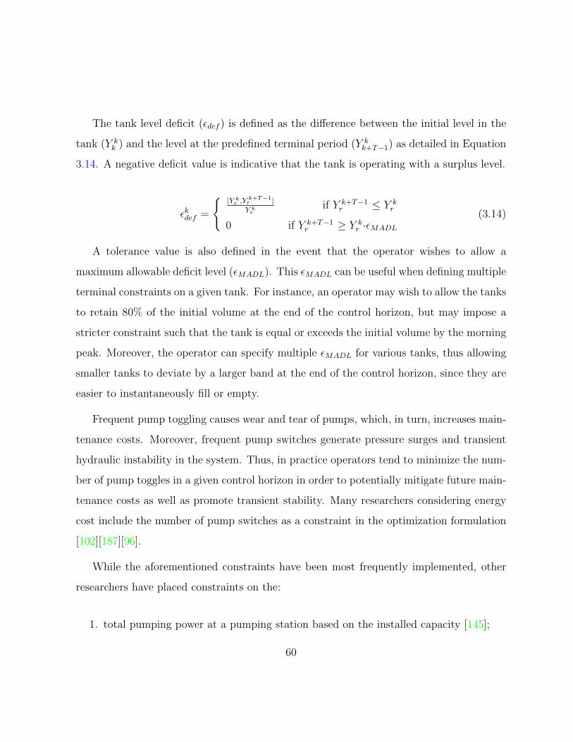
The tank level deficit (εdef ) is defined as the difference between the initial level in the
tank (Y kk ) and the level at the predefined terminal period (Y k
k+T−1) as detailed in Equation
3.14. A negative deficit value is indicative that the tank is operating with a surplus level.
εkdef =
{ |Y kr ,Y k+T−1
r |Y kr
if Y k+T−1r ≤ Y k
r
0 if Y k+T−1r ≥ Y k
r ·εMADL
(3.14)
A tolerance value is also defined in the event that the operator wishes to allow a
maximum allowable deficit level (εMADL). This εMADL can be useful when defining multiple
terminal constraints on a given tank. For instance, an operator may wish to allow the tanks
to retain 80% of the initial volume at the end of the control horizon, but may impose a
stricter constraint such that the tank is equal or exceeds the initial volume by the morning
peak. Moreover, the operator can specify multiple εMADL for various tanks, thus allowing
smaller tanks to deviate by a larger band at the end of the control horizon, since they are
easier to instantaneously fill or empty.
Frequent pump toggling causes wear and tear of pumps, which, in turn, increases main-
tenance costs. Moreover, frequent pump switches generate pressure surges and transient
hydraulic instability in the system. Thus, in practice operators tend to minimize the num-
ber of pump toggles in a given control horizon in order to potentially mitigate future main-
tenance costs as well as promote transient stability. Many researchers considering energy
cost include the number of pump switches as a constraint in the optimization formulation
[102][187][96].
While the aforementioned constraints have been most frequently implemented, other
researchers have placed constraints on the:
1. total pumping power at a pumping station based on the installed capacity [145];
60

2. source flowrates and velocities [140]; and
3. warnings produced by the EPANET2 hydraulic simulator for infeasible hydraulic
conditions [96].
While constraints are typically handled via penalty functions, these methods inadver-
tently introduce subjectivity into the optimization formulation. This is because penalty
functions generate a trade-off between constraint violations and objective function values.
Specifically, lower penalty parameter values would allow large constraint violations in re-
turn for small reductions in the objective value, meanwhile higher penalty parameter values
would require a larger decrease of the objective value to compensate for the same amount
of constraint violation [96].
As such, in this research, constraint violations were handled using a modified version of
the penalty-free candidate solution ranking approach [41]. This method quantifies the rela-
tive magnitude of constraint violations for infeasible solutions so that the relative quality of
two infeasible solutions can be compared [41]. The constraint handling process implements
the following logic:
1. between two infeasible solutions, the one with the least total violations is always
assigned a better objective function value;
2. between an infeasible and a feasible solution, the feasible one is always assigned a
better objective function value; and
3. between two feasible solutions, the one which is less costly is always assigned a better
objective function value.
61

3.5 Control Variable Formulation
With the objective of manipulating pump operations over the duration of the control
horizon, a number of mathematical representations may be used to encapsulate an arbitrary
pump control setting (hereby referred to as a pump schedule). For fixed speed pumps, a
pump schedule is designed to represent the hours during a control horizon that a pump
is either on or off. Meanwhile for variable speed pumps, pump schedules should capture
the speeds at which the pump should be operated at during the control horizon. As such,
pump schedule representations should be carefully selected based on the physical type of
pumping system they are meant to control (i.e. variable speed pumps versus fixed speed
pumps), as well as the design and objective of the control scheme.
In this research, a number of explicit pump schedule representations for the purpose of
real-time control are formulated and evaluated. These include:
• Binary and discrete status control; and
• Modified Time controlled Triggers
The formulation of implicit pump schedules, such as level-based control, are omitted
in this research since these represent reactive control strategies. In addition, this research
formally introduces a novel modification to the above representations in order to enhance
the stability of the real-time controller.
3.5.1 Binary and Discrete Status Control
Binary Status Control (BSC) is the most commonly used explicit formulation of pump
schedules both in the context of offline optimization [102][193][60] and real-time control
62

[145][81][171][111][158]. As suggested by its name, BSC represents the schedule of an
arbitrary pump as a binary sequence with dimensions equal to the length of the control
horizon. Specifically, the control horizon is discretized into Nt equal intervals. During each
interval, the status of the pump is assumed to be held constant. The status during each
interval is thus a decision variable that can be manipulated by the optimization algorithm.
Intuitively, a single binary value is used to represent the pump’s status during each interval,
whereby active and idle statuses are indicated with values of one and zero, respectively.
Figure 3.6 provides an example of how to map an arbitrary 24-hour schedule for a single
pump with the BSC representation.
Figure 3.6: Mapping an arbitrary pump schedule to Binary Status Control formulation
Depending on the desired resolution of control, the operator can specify the size of each
interval (i.e. hourly, 30 minutes, 15 minutes etc.). However, the size of the sequence, and
thus the memory required, increases with increasing resolution.
63

The BSC representation can be modified to provide the flexibility of being able to
capture the behaviour of both fixed and variable speed pumps as detailed in Equation
3.15. For variable speed pumps, each decision variable in the sequence can be formulated
as either a discrete variable from a fixed set of integers, known as Discrete Status Control
(DSC) [90], or alternatively as a continuous variable bound by 0 and 1. In the former, the
fixed set of discrete integers represent the range of allowable speeds (that the pump can
operate at), the latter suggests that the speeds may be toggled as some fraction of the
maximum capacity.
Udisci ∈ [0, 1, ..., Nsp]{
U conti ∈ R | 0 ≤ U cont
i ≤ 1}(3.15)
While the Binary and Discrete formulations provide the flexibility of representing both
types of pumping systems, there exist a few challenges in its implementation. Most no-
tably, neither representation has any mechanism to explicitly control the number of pump
toggles that occur in the control horizon. As such, this formulation is prone to generating
hydraulically infeasible solutions over the optimization search trajectory. Moreover, the
BSC and DSC formulations are computationally intensive. This is because an array size of
at least Nt is required to represent a Nt-sized control horizon. As such, the decision space
grows at a rate of 2Nt∗Np as Nt and Np are increased. This computational intensity creates
a barrier for real-time implementation time in large network systems with a significant
number of pumps to control.
64

3.5.2 Time Controlled Triggers
An alternative to the status based formulations involves representing pump schedules as a
function of the time spent active or idle. This concept was initially introduced for offline
pumping optimization by [157] and [115], but was then formally defined by [25] and [96].
In their proposed formulation, the number of consecutive hours a pump is active and then
subsequently idle is encoded in a sequence of integer pairs [Ui, Ui+1] called Time Controlled
Triggers (TCT). As such, each TCT pair represents a pump switch. In this manner, the
number of pump switches can be explicitly managed in the TCT formulation simply by
defining the number of consecutive active and idle pairs.
Figure 3.7: Mapping an arbitrary pump schedule to the TCT formulation
Figure 3.7 provides an overview of how to map a hypothetical 24-hour schedule for a
single pump to the TCT formulation.In this hypothetical example, there is a maximum of 6
allowable pump switches and this constraint is implictly handled with 6 decision variables.
The range of each decision variable in the TCT sequence depends on the desired reso-
65

lution of control. Using discrete values, an hourly resolution can be achieved by limiting
the bounds to [0,24], whereas a 15-minute or 30-minute resolution can be achieved with
bounds of [0,96] and [0,48], respectively. To be consistent with the binary representation,
we assume an hourly control resolution over a 24-hour control horizon in this research.
Moreover, the TCT formulation can accommodate the scenario whereby a given pump
uses less than the maximum number of pump switches. This is demonstrated in Figure 3.8
whereby zeros are placed in all subsequent elements in the sequence to represent unchanged
statuses.
Figure 3.8: Handling single pump with fewer than maximum allowable switches
Equations 3.16 and 3.17 describe how the TCT representation can be formulated math-
ematically for a single pump. Assuming that a maximum allowable number of switches,
Smax, is permitted, the total number of decision variable pairs is thus Smax.
U = [U1, U2, ..., USmax ] (3.16)
66

U1 ∈ [0, Tctrl]
Ui ∈ [0, Tctrl,
i−1∑j=1
Uj], ∀i ∈ 1, ..., Smax
(3.17)
Note that the sum of all elements in the TCT sequence must sum up to the total
number of hours in the control horizon (Tctrl) as shown in 3.18.
Smax∑i=1
Ui = Tctrl (3.18)
In this manner, the individual decision variables in the TCT sequence are not indepen-
dent. The subscript ’i’ denotes the sampling order through which the decision variables are
perturbed. As such, the decision variable denoted by i=1 does not necessarily represent the
first decision variable in the TCT sequence, rather it represents the first randomly drawn
sample.
The primary motivation for the TCT formulation is to overcome some of the limitations
of the binary status formulation whereby the maximum number of pump switches is not
explicitly handled. By representing a pump schedule by the maximum number of allowable
switches, the TCT formulation does not allow for exceedances in pump switches during a
particular control horizon. This formulation ensures that a greater fraction of the decision
space is feasible. Moreover, since the number of pump switches is necessarily a fraction of
the hours in a given control horizon (typically 3-6 pump switches are allowed in operations),
the decision space size is greatly reduced. To reinforce this notion, consider a single pump
that must be scheduled over a 24-hour control horizon with an hourly resolution. Since the
binary status formulation allows for a pump to have one of two possible states at every hour,
the size of the decision space for the control horizon is 224 or 16,777,216 possible options.
67

However, if the number of pump switches is restricted to six (Nsw ≤ 6), as depicted in
Figure 3.7, the size of decision space is reduced to 5,408,312 feasible options [98]. As such,
by using the TCT formulation to explicitly limit the number of pump switches, the decision
space (number of solutions) is reduced in size by 67% relative to the binary status control
approach. The computational effort required to generate and handle a large number of
pumps in complex networks is significantly less intensive than the binary formulation.
However, there exist a few limitations with the TCT formulation. Firstly, this formula-
tion is unable to represent variable speed pumps since each element represents the number
of hours a pump is active or idle. Moreover, while the TCT formulation effectively con-
strains the number of pump switches during a given control horizon, in a real-time context,
it has no memory of previously incurred switches and may thus lead to decision variable
solutions that are optimal and feasible in the current control horizon, but infeasible in the
overall trajectory of the day.
3.6 Feedback Formulation
In this research, the previously described pump schedule representations are reformulated
for real-time control applications. Specifically, the definition of a novel feedback repre-
sentation is formalized. The feedback representation is designed as an alternative to the
traditional feedforward real-time pump scheduling methods commonly proposed in liter-
ature [145][81][158][111][125]. In feedforward scheduling, a pump schedule is produced at
every control timestep (1 hour) for the duration of a predefined control horizon (typically
24 hours). The primary limitation of this feedforward scheduling approach is that, at each
timestep, the proposed schedule is unaware of the number of pump switches that have
already occurred in the past since it is not formulated to encapsulate any short-term mem-
68

ory of the system. The immediate consequence of this limitation is that it may lead to
situations where the total number of switches in a day violates the maximum allowable
limit. However, only one study [125] realized this limitation, but none have incorporated
this feedback awareness directly into the optimization formulation.
While at every timestep the proposed schedule is necessarily feasible during the current
control horizon, the total number of switches in a given calendar day remains uncon-
strained. This phenomenon is illustrated in Figure 3.9. The net result is that as the
real-time controller proceeds forward in time, it may lead to oscillatory behaviour and
transient hydraulic instability, in terms of pressure surges and backwater effects in the
system.
Figure 3.9: Motivating the Feedback Scheduling Paradigm
The proposed feedback scheduling method is designed to address these limitations by
explicitly encapsulating short term memory into the decision variable formulation at every
control timestep. This method is conceptually agnostic to the representation of the decision
variable sequence and can thus be easily adapted to binary status control to represent
variable speed pumps. However, in this section we demonstrate the formulation with the
previously defined TCT formulation. As such, the newly reformulated TCT variables are
69

hereby referred to as Feedback-Time Controlled Triggers (F-TCT).
Figure 3.10: Decomposition of control horizon into operating and planning horizon
The control horizon T ctrl was previously defined as the sequence of T discrete control
time steps (hours) used during the real-time optimization process. In other words, it is the
duration of time that a pump is scheduled for (i.e. 24 hours). In the feedback formulation,
this control horizon is decomposed into two smaller subsets: the operating T oper and plan-
ning horizons T plan, as shown in Figure 3.10. The operating horizon represents the number
of hours in the control horizon that are part of the current calendar date. That is to say,
the fraction of the pump schedule that occurs in the current calendar day. Meanwhile, the
planning horizon represents the duration of hours in the control horizon that occur outside
the current calendar day, and thus encapsulate the hours in the pump schedule that are
being planned beyond the current operational shift. As such, the total number of hours in
both the operating and planning horizons must necessarily sum up to the total hours in the
control horizon. Moreover, the number of hours in the operating horizon must equal the
difference between the total hours in the control horizon and the number of elapsed hours
T elaps in the current day. The planning horizon is thus equal to the number of elapsed
hours in the current day. This definition is further described mathematically in Equation
70

3.19.
Tctrl = 24, 0 ≤ Telaps ≤ 23
Toper + Tplan = Tctrl
Tplan = Telaps
(3.19)
By decomposing the control horizon into operating and planning horizons, short-term
memory of the current calendar date’s trajectory can be explicitly encoded into the decision
variable formulation. Since the total elapsed switches (Selaps) in a given day up until the
current timestep are known, the remaining allowable switches in the current day are also
known. As such the remaining switches can be used as an upper bound on the maximum
allowable switches in the operating horizon (Soper). In this manner, the operating horizon
decision space is dynamically adjusted based on the elapsed trajectory of pump switches
in the day. With this formulation, the number of switches encountered in a given calendar
date never violates the predefined maximum. As such, the total allowable switches (Smax)
in the control horizon must equal the arithmetic sum of number of switches allocated both
in the operating and planning horizons (Splan). This notion is further defined in Equation
3.20.
Soper = Smax, Selaps, Soper ∈ [0, Smax]
Splan = Smax, Soper = Selaps, Splan ∈ [0, Smax]
(3.20)
Adopting the F-TCT formulation, the decision variable (U) sequence is now decomposed
into operating and planning subsets of sizes (Soper) and (Splan), respectively. In each
subset, the maximum number of hours available for allocation is equal to T oper and T plan,
respectively. With this decomposition, the decision variable size is unchanged relative
71

to the standard feedforward TCT formulation. Equation 3.21 describes how the F-TCT
representation can be formulated in vector format, meanwhile Equation 3.22 demonstrates
how each element in the vector sequence is calculated mathematically. Note that each
subset of F-TCT sequence follows the previously defined TCT sampling archetype.
U = [U oper, Uplan]
U oper = [U1, U2, ..., USoper ]
Uplan = [U1, U2, ..., USplan ]
(3.21)
U oper1 ∈ [0, T oper], Uplan
1 ∈ [0, T plan]
U operi ∈ [0, T oper,
i−1∑j=1
Uj], ∀i ∈ 1, ..., Soper
Uplani ∈ [0, T plan,
i−1∑j=1
Uj], ∀i ∈ 1, ..., Splan
(3.22)
Note that the sum of all elements in each F-TCT subset must sum up to the total
number of hours in its respective horizon, as detailed in Equation 3.23.
Soper∑i=1
Ui = T oper,Splan∑i=1
Ui = T plan (3.23)
In this manner, the individual decision variables in the F-TCT sequence are not inde-
pendent. At each jth sampling instant, the jth decision variable is constrained by zero and
the total unallocated hours in the horizon. Similar to the TCT formulation, the decision
variable denoted by i = 1 does not necessarily represent the first decision variable in the
F-TCT sequence, rather it represents the first randomly drawn sample. Moreover, the
decision variable sampling sequences in both subsets are independent of each other, that
72

is to say, the sampling order in the operating sequence does not influence the order in the
planning horizon and vice versa.
An example representation of the F-TCT formulation is provided in Figure 3.11. In
this example, the previously presented hypothetical schedule (Figure 3.7) for a single pump
is used. The number of elapsed hours is assumed to be 11 in this example (i.e. the current
timestep is 11AM), with 6 maximum allowable switches. In this example, 3 switches have
already elapsed. As such, the decision variable sequence size for both the operating and
planning horizons is restricted to 3 each. Given that 11 hours have elapsed, the number
of hours available for allocation in the operating and planning horizons is 13 (from 11AM
- 12AM, exclusively) and 11 (12AM - 10AM, the subsequent day), respectively. This can
be seen by simply summing the elements in each subset.
Since this new formulation is dependent on the system’s short-term history of pump
scheduling, a few boundary conditions need to be imposed to prevent instability in the
system, in the event of anomalous scenarios. These conditions may occur in the following
cases where:
1. a pump has used none or a small fraction of allowable switches throughout the ma-
jority of the current calendar date; and
2. a pump has used all of its allowable switches during the current calendar date.
In the former condition, the controller is at risk of recommending a large number of
switches within a short duration of time, particularly at the end of the calendar day, thus
leading to oscillatory behaviour and transient instabilities. In the latter, the controller
must be informed to no longer allow any pump switches in the operating horizon in order
73

Figure 3.11: Formulation of feedback time-control triggers
to prevent a constraint violation. As such, the last known status of the pump is held
constant until the end of the operating horizon.
As such, various sub-processes are defined to prevent frequent oscillations in pump
statuses. Specifically, two ’If-Then’ conditional statements were encoded as part of the
stability analysis. These are described in Table 3.1. Condition 1 describes the course of
action if the operating horizon is less than or equal to the maximum number of switches
and the number of allowable operating switches is non-zero. In this case, the controller sets
the available number of operating switches to zero, thus preventing the pump from toggling
statuses during remainder of operating horizon. The remaining switches are reallocated to
the planning horizon.
74

Table 3.1: Conditional Statements for Stability Control
Index Condition (IF) Action (THEN)
1 Toper ≤ Smax and
Soper > 0
Soper = 0; Splan = Smax,
CONSTANT[k] = True
2 Toper ≤ Tctrl
2and
Soper ≥ Toper
Smax
Soper = Toper
Smax;
Splan = Smax, Soper
In the event that the operating horizon is less than or equal to half the control horizon
and the allowable number of operating switches exceeds the operating horizon divided by
the maximum number of switches, Condition 2 is triggered. In this event, the number
of allowable operating switches is scaled proportionally to the number of hours in the
operating horizon divided by the maximum number of switches. Figure 3.12 describes
the algorithmic pathway for implementing the feedback scheduling formulation for F-TCT
decision variables.
The first sub-process involves processing the elapsed trajectory information and storing
it in memory for subsequent use. Specifically, the total number of elapsed switches, the
number of allowable switches in the operating and planning horizons, the number of hours
in the operating and planning horizons are determined.
Once this preliminary information is stored, the elapsed trajectory information is
screened for boundary conditions. These conditions include occurrences when either the
operating or planning horizons are zero, at the beginning and end of the calendar day,
respectively. In these conditions, the standard TCT formulation is used since no trajec-
tory information is required. A second round of screening is done for stability handling
75

Figure 3.12: Flowchart of feedback formulation sub-processes
using the previously described conditional statements. In the event that the conditions are
triggered, the trajectory information is overwritten to scale the allowable switches in the
operating horizon accordingly.
Finally, once the allowable switches for both the operating and planning horizons have
been allocated, this information alongside the horizons are encoded compactly for use in
the optimizer’s selection and perturbation algorithm. These algorithms will be described
in detail in the subsequent chapter.
76

Chapter 4
Optimization Engine
In this research, an optimization algorithm is required to guide the generation of real-time
pump schedules that are not only adaptive to the current hydraulic conditions of the system
but are also near-optimal in order to drive down energy costs over the control horizon. As
such, this section begins with an overview of the most commonly applied optimization
algorithms for water resource applications. Given the nonlinearity and complexity of the
systems under investigation, we omit traditional derivative-based solvers from this review
and focus on metaheuristic optimization methods.
As defined by [208], a metaheuristic is an iterative generation process which intelligently
leverages different learning strategies to effectively explore the search space of a particular
problem and find near-optimal solutions. Unlike traditional optimization algorithms which
rely on derivative-based methods to localize optimal values of objective functions, meta-
heuristics incorporate structured randomness for search and follow empirical guidelines,
often motivated by observations of natural phenomena, or an inherent understanding of
the system being studied [104].
77

The primary advantages of using metaheuristics over traditional derivative based solvers
include the ability to:
• solve problems with complex, non-linear mathematical properties [150]. Most tradi-
tional methods are unable to deal with nonlinearities, discontinuities and multi-modal
response surfaces;
• perform both global and local searches of the fitness function, increasing the chances
of finding near-optimal solutions to complex problems [118]; and
• easily integrate with simulation models bypassing the need to simplify or reduce the
problem (i.e. via linearization).
Broadly speaking, metaheuristic optimization methods can be categorized into two
groups including population-based and single solution based methods [104]. The former
include algorithms that generate and evolve a population of candidate solutions. Popular
examples of these algorithms include but are not limited to genetic algorithms (GAs), par-
ticle swarm optimization (PSO) and ant colony optimization (ACO). Meanwhile, the latter
includes algorithms that generate and evolve a single candidate solution. Popular examples
of these algorithms include but are not limited to simulated annealing, Tabu-search, and
various other trajectory or local search methods. In this chapter, both categories will be
discussed for use in the context of real-time control and optimization of WSDs.
4.1 Overview of Population-based Optimization
Genetic Algorithms have been the most commonly applied metaheuristic optimization
method within water resources applications. At a high level, they apply the Darwinian
78

concept of natural selection to select and evolve candidate solutions with the highest ’fitness
values’ thus converging to the ’fittest’ solution.
Figure 4.1: Generalized workflow of Genetic Algorithms
According to [122], GAs can be broadly characterized by the following generalized
elements:
1. generation of an initial population of potential solutions known as chromosomes;
2. computation of a fitness metric for each chromosome;
3. ranking of chromosomes according to metric;
4. selection of candidate solutions to participate in a mating operator, where information
from two or more parent solutions are combined to create offspring solutions; and
5. mutation of each individual offspring to maintain diversity and prevent premature
convergence to local optima.
These elements are executed iteratively for a predefined computational budget, known
as generations, or until a suitable solution is determined. The underlying principle of this
method is that candidate solutions with high fitness values contain specific characteristics
79

in their ’chromosomes’ that are important for optimizing the objective function [122].
As such, by mating high-performing parent candidate solutions, it is expected that the
produced offspring may attain superior characteristics relative to their parents. In this way,
the algorithm simulates survival of the fittest objective function values, without requiring
derivative information [59].
However, the obvious limitations in the application of population-based algorithms (e.g.
GA and PSO) is that they require significant computational-overhead for the reproductive
cycle of populations and evaluation of fitness functions for every individual [3]. Moreover,
sub-processes such as selection, mating and mutation require further subjective decision-
making and parameter tuning.
4.2 Requirements for Real-time Optimization
The ’No Free Lunch’ theorem, proposed by [196], stipulates that an optimization algo-
rithm capable of consistently outperforming all other algorithms for all classes of problems
simply does not exist. As such, this research does not aim to qualify the selection of an
optimization algorithm based on results demonstrated in literature. Rather, the necessary
structural requisites of an algorithm for the specific purposes of RTC are listed and used
to guide the selection of a suitable algorithm. These include:
1. Flexibility - an ability to handle both continuous and discrete decision variables;
2. Scalability - an ability to handle large decision spaces (50 - 100 decision variables);
3. Explorative - an ability to conduct both Global and local searches;
80

4. Computational efficiency - Rapidly converge to a near-optimal solution without sig-
nificant computational overhead;
5. Parsimony - optimization algorithm requires no parameter tuning - all parameters
are well-defined;
6. Ease of Use - modularly designed and can easily integrate with simulation model
within an RTC platform.
As mentioned in the previous chapter, pump schedules can be formulated as either
discrete or continuous decision variables. As such, the required optimizer must be able
to conduct elementary operations such as processing, selection and perturbation on both
discrete and continuous variables. Moreover, given that a real WSD system is likely to
have dozens of pumps (often exceeding 50), the optimizer should be able to handle large
decision spaces for the generation and evolution of decision variables during the search
trajectory. These needs immediately eliminate the possibility of using traditional solvers.
Since a simulation model is required to calculate the impact of control variables on the
objective function, the optimization method should be able to easily integrate with a sim-
ulation model. Moreover, given that model execution times can range anywhere between
1-30 seconds, the computational efficiency of the algorithm is necessarily bottlenecked by
the execution time. The algorithm should thus be easily parallelizable or able to converge
to good solutions rapidly (with a constrained computational budget). This means the opti-
mizer should be able to produce meaningful results within the reporting frequency specified
by the decision-maker. While this is ultimately a function of the problem formulation and
the complexity of the simulation, the optimizer type can greatly influence performance.
As such, Population-based algorithms are deemed as unsuitable candidates for RTC. This
81

is because they require significant computational-overhead for the reproductive cycle of
populations and evaluation of fitness functions for every individual (Alba et al., 2013).
Lastly, an optimization algorithm should be able to perform both exploration (i.e.
global search) and exploitation (i.e. local search) of the fitness function, increasing the
chances of finding near-optimal solutions to complex problems [118].
4.3 Dynamically Dimensioned Search
Based on the aforementioned criteria for RTC applications, a dedicated optimization algo-
rithm, namely the Dynamically Dimensioned Real-time Scheduling (DD-RTS) algorithm
was developed. The DD-RTS algorithm is the real-time extension of the Dynamically Di-
mensioned Search (DDS) algorithm, initially introduced by [185]. DD-RTS is specifically
designed to efficiently generate candidate control variable settings for the real-time control
and optimization of water resource infrastructure. DDS is a novel and simple stochastic
single-solution based heuristic global search algorithm that was developed for the purpose
of finding good global solutions (as opposed to globally optimal solutions) within a specified
evaluation budget [185]. The algorithm is designed to scale the search to the user-specified
number of function evaluations and thus has no other stopping criteria. In this manner, it
is well suited for real-time control applications where the stopping-criteria is constrained
by the user-specified reporting frequency.
In summary, the algorithm searches globally at the start of the search trajectory and
becomes a more local search as the number of iterations approaches the computational
budget. The adjustment from global to local search is achieved by dynamically scaling the
number of dimensions in the neighborhood. This dynamic scaling is adjusted stochastically
throughout the search trajectory by reducing the number of dimensions to include in the
82

neighborhood at every iteration. Note that the neighborhood is defined as the subset of
decision variables that are selected to be perturbed, i.e. modified from their current best
value. This search trajectory is designed to match the human decision-making behaviour
that may occur in operations, whereby an operator starts by changing many control vari-
ables and then iteratively refines these variables until converging onto an optimal set.
The DDS algorithm suite considered in this research consists of:
1. the continuous, single objective version of DDS [185]; and
2. the discrete version of DDS (HD-DDS) [183].
HD-DDS is a discrete extension to the simple and efficient DDS algorithm [185].The
primary difference between DDS and HD-DDS is that the discrete nature of the decision
variables must be accounted for in the neighborhood perturbation step of the original
DDS algorithm. In HD-DDS, these perturbation magnitudes are randomly sampled from
a discrete probability distribution that approximates a normal distribution with a mean of
zero [183]. The perturbation strategies from both DDS and HD-DDS are adapted in the
real-time extension, DD-RTS.
In this chapter, the necessary modifications that were added to the real-time extension
of DDS, DD-RTS, are discussed in detail. These include:
1. Modified Search Heuristics, whereby the neighborhood selection and perturbation
techniques are adapted specifically for the purpose of real-time scheduling;
2. Computational Efficiency Methods, whereby parallelization, warm-start initialization
and pre-emption techniques are adopted for improving the runtime of the optimiza-
tion algorithm for real-time implementation;
83

3. Simulation Model integration, whereby the necessary application programming in-
terfaces (API) for communicating with the EPANET2 simulation model within a
real-time optimization framework are developed.
4.3.1 Search Heuristic
The DD-RTS algorithm is designed to generate near global optimal control variable settings
within the predefined reporting frequency of the real-time controller, following a modified
DDS heuristic. Recall that the core heuristic elements of the DD-RTS algorithm can be
generalized as shown in Figure 4.2.
Figure 4.2: Generalized workflow of DDS Algorithms
In the DD-RTS algorithm, the decision variables of the optimization problem are defined
using the control variable representations described in Chapter 3. When using the F-TCT
and TCT formulations, each time trigger element in the pump schedule is treated as its
own decision variable. For example, if a hypothetical system has only 5 pumps with 6
maximum allowable switches per pump, then the system has 30 decision variables in total.
Similarly, in the binary representation each hour in the schedule is treated as a decision
variable. For the same hypothetical system, the binary representation would yield a total
of 120 decision variables.
84

In DD-RTS, the generalized heuristic is extended as detailed in Figure 4.3, given the
F-TCT formulation. Note that the initialization, neighborhood selection and perturbation
strategies are conducted independently for each pump in the system.
Figure 4.3: Workflow of DD-RTS Algorithm
The algorithm starts by initializing all decision variables with a warm solution. In the
context of real-time control, a warm solution is a near-optimal solution for a historical day
that has a similar disturbance (demand) profile [134]. The definition of warm solution can
also be broadened to include any approximate initial pump schedule. Results for similar
days either that occurred recently or from a prior year near the same date are likely near
optimal. This is because demand patterns within a given season do not significantly vary
85

from one another. As such, previously developed optimal solutions can be archived for
initialization. An alternative method to generate warm solutions involves using the con-
temporaneous pump schedule of a previous control timestep. Lastly, to generate schedules
that are fairly consistent, the pump schedules at every control timestep may be initialized
with the contemporaneous schedule produced at the first hour of the day (hour 0). In doing
so, the optimizer will not likely significantly deviate from the optimal solution generated
at hour 0, except in the event that an anomalous condition arises. This form of warm start
is particularly attractive for creating schedules that do not significantly change at every
timestep in a given day, a feature that may be particularly attractive for an operator.
Once a warm solution is initialized, it must also be validated when using the F-TCT
formulation to ensure that the prescribed allowable switches for both the operating and
planning horizons are not violated. This process involves simply enumerating the total
number of switches encountered in the warm solution during each horizon (Sk) and then
evaluating whether they fall within the allowable thresholds (Smax). In the event that the
number of switches in one of the horizon exceeds the maximum allowable limit (Nexc > 0),
then the smallest status in that horizon, denoted by argmin(X), are collapsed until the
limit is satisfied. The rationale for selecting the smallest statuses was to remove switches
that are likely to have minimal impact on the overall system schedule. Once the smallest
statuses have been removed from the schedule, the remaining unallocated hours (valj) are
spilled onto the adjacent statuses. For example, if a pump was active for 8 hours and then
idle for the next 2 hours (the minimal value in the schedule), then the two hours are spilt
onto the active status - resulting in a schedule where the pump is on for 10 hours. This
process is repeated until all exceedances in the maximum number of switches are removed
from the schedule.
This process of collapsing exceedances in the maximum number of switches is detailed
86

mathematically in Equation 4.1.
Sk > Smax → Nexc = Smax − Sk ∀k = [oper, plan]
Nexc > 0→ indj = argmin(X); valj = min(X)
Xprem,j = φ; Xp
ind,j+/−1 = |valj|
∀j = 1, ..., |Nexc|
(4.1)
Once initialized, the selection and perturbation strategies are initiated for each pump
in the system, as detailed in the pseudo-code provided in Figure 4.4.
Figure 4.4: Pseudo-code of DD-RTS Heuristics
87

The process of including decision variables in the neighborhood of perturbation involves
defining two stochastic variables, the probability of including decision variables (Pincl) and
the current perturbation probability (Ppert). The probability of perturbing a given decision
variable (Ppert) in the neighborhood is a scalar value and is stochastically driven by the
current progress in the optimization process as detailed in Equation 4.2.
Ppert =log(i)
log(N)(4.2)
whereby i is the current iteration and N is the maximum number of iterations. In DD-
RTS, each pump is selected into the neighborhood and perturbed independently of other
pumps. As such, Pincl is a matrix of size NP x NS, whereby NP is the number of pumps
and NS is the number of allowable switches. Each entry is sampled from the continuous
uniform distribution. This process guarantees that each pump has equal probability of
selection for perturbation at every iteration of the search trajectory, contingent on the
current perturbation probability. At every iteration, the elements that are smaller in value
than Ppert are filtered and included in the neighborhood. Through this mechanism, fewer
decision variables are included in the neighborhood at every iteration.
Once the subset of decision variables has been selected for inclusion into the neighbor-
hood, candidate control variables are created by perturbing each decision variable in the
neighborhood. Note that DDS is a greedy algorithm and thus only perturbs the current
best candidate solution at every iteration.
If the neighborhood for perturbation is non-empty, the perturbation process is initiated
iteratively for each pump. As shown in the pseudo-code in Figure 4.4, the first step involves
determining the total number of hours in the schedule that are static (Tstatic) and will not
be perturbed as part of the algorithm. This is achieved by enumerating the total number of
88

hours attributed to decision variables that are not included in the neighborhood (NC). In
doing so, the total number of hours remaining that are available for perturbation (Tremain)
are easily determined by subtracting the fixed hours (Tstatic) from the total hours in the
control horizon (Thorizon). Note that the sum of all elements in the neighborhood for a given
pump must necessarily equal the total number of hours available for allocation (Tremain) for
the same pump. Once the bounding conditions for perturbation are known, each decision
variable for a given pump is normalized by the maximum available hours (Tremain) for
the same pump. This ensures the decision variable is scaled to the continuous domain as
bounded by [0,1].
Once the decision variable has been scaled, the standard DDS perturbation strategy for
continuous variables is deployed. These perturbation magnitudes are randomly sampled
from a normal distribution with a mean of zero and constant variance, as detailed in
Equation 4.3 [185].
xnew(i,j) = xcurr(i,j) + σ(i,j)N(0, 1);
σ(i,j) = r(xmax(i,j) − xmin
(i,j))
xmax(i,j) = 1, xmin
(i,j) = 0
(4.3)
Note that xnewij and xcurrij represent the newly perturbed and current best decision
variable, respectively. The subscript i represent the time trigger index as part of the TCT
or F-TCT sequence, meanwhile the subscript j represents the pump being scheduled. The
only algorithm parameter to set in the DDS algorithm is the scalar neighborhood size
perturbation parameter (r) that defines the random perturbation size standard deviation
as a fraction of the decision variable range. However, this parameter is well-defined and
does not require any tuning [185]. In the event that xnewij falls outside the acceptable range
of the decision variable [0,1], it is reflected using the techniques described in [185].
89

Recall that when perturbing decision variables as part of the TCT and F-TCT control
variable formulation, the sum of all time triggers in the sequence (pump schedule) must
sum up to the total number of hours in the control horizon. In this manner, the individual
decision variables in the TCT sequence are not independent. This is particularly evident
once the decision variables are rescaled back to the original discrete domain after perturba-
tion. Given the dependency of each decision variable in the neighborhood, it is important
to control the order in which each decision variable in the neighborhood is perturbed.
Perturbing decision variables in the same order at every iteration leads to schedules that
are biased, since each decision variable will have a non-constant perturbation variance.
The consequence of bias schedules is that they may be inadvertently biased towards ac-
tivating pumps during unfavourable hours (such as peak periods) or deactivating pumps
for large periods of time. The influence of the sampling order on perturbation magnitude
distribution in a given optimization trajectory is detailed in Figure 4.5.
As shown in Figure 4.5, the first decision variable, denoted by U1, exhibits the expected
distribution shape. Note that the distribution only contains a large number of zero values
since negative hours are not possible and are thus bounded by zero. However, it is clear
that each decision variable in the sequence exhibits a drastically different perturbation
distribution.
In an idealized perturbation strategy, each decision variable in the given pump schedule
should have a similar perturbation magnitude distribution, thus ensuring that each variable
is not preferentially selected for a certain value. This problem can be easily addressed by
simply shuffling the perturbation sampling order of the neighborhood at every iteration
with random permutations of the indices. The result of this shuffled sampling order is
demonstrated in Figure 4.6.
90

Figure 4.5: Perturbation of TCT decision variables without randomized sampling order.
Example pump is displayed with 6 decision variables, whereby each decision variable was
initialized with a current best solution value of 4 hours
4.3.2 Parallelization Strategy
Parallel evolutionary algorithms have been extensively investigated in the literature, hav-
ing been applied to water distribution systems [50]; hydrological model calibration prob-
lems [48][180][204]; and groundwater management [180][88][149]. For example, [37] devel-
oped a parallel genetic algorithm library (PGAPACK) in FORTRAN by coupling cluster
based parallel computing with the Non-Dominated Sorting Genetic Algorithm II (NSGAII)
[42] to calibrate a 139 parameter hydrological model of the Calapooia watershed. Simi-
larly, [180] tested a parallelized version of the Epsilon-NSGAII with the Argonne National
91

Figure 4.6: Perturbation of TCT decision variables with randomized sampling or-
der.Example pump is displayed with 6 decision variables, whereby each decision variable
was initialized with a current best solution value of 4 hours
Laboratory’s Infinicon MPI on a Linux cluster for the SAC-SMA model and a long-term
groundwater monitoring (LTM) application. In summary, these studies demonstrated that
by using parallel computing associated with optimization, solutions can be improved and
computation times can be reduced dramatically. However, the obvious limitations in the
applications lie in the implementation of population-based algorithms (e.g. GA, SCE,
PSO, etc.) which require significant computational-overhead for the reproductive cycle of
populations and evaluation of fitness functions for every individual [2]. DDS has at least
three advantages relative to these algorithms:
92

1. it has an immediate efficiency advantage because it is not population-based;
2. it is designed to find good solutions quickly and thus it adjusts to the user-specified
computational scale to generate good solutions without requiring any algorithm pa-
rameter adjustment; and
3. it has only one algorithm parameter that is easily interpreted and has a well-established
default value that has been shown to produce good results over a range of test prob-
lems. No algorithm parameter fine-tuning is required.
To promote flexibility in end-user adoption, the Dynamically Dimensioned Search
(DDS) algorithm suite described in the previous subsection was parallelised for both shared
memory (local multi-core desktop applications) and distributed memory (high performance
computing clusters) architectures using the Message Passing Interface (MPI). The MPI
library is a collection of subroutines that allows parallel computational nodes to com-
municate with each other by transmitting and receiving messages. MPI is recognised as
the standardised approach to programming heterogeneous memory systems including both
shared memory within a single node as well as distributed memory across multiple nodes
[79].
For the purpose of environmental optimization, the MPI model typically exploits the
Single Program Multiple Data (SPMD) construct to simultaneously execute multiple sim-
ulation runs (with unique parameter sets) using the same single optimizer and model
executable. In this study, the ’single program’ refers to the previously described DDS al-
gorithm Suite. The SPMD construct is advantageous because it allows for point to point
communication between nodes, as well as asynchronous and transparent message trans-
ferring. The asynchronous nature of message passing is particularly advantageous in the
context of the DDS algorithm suite as it serves to minimize idling-time. Note that unlike
93

threads, MPI uses a statically allocated group of computational nodes which are defined
at the beginning of program execution. Each node is assigned a unique identifier called a
’rank’ for identification purposes.
A typical HPC architecture comprises a cluster of nodes interconnected via a high-
throughput, low latency network. As such, using a system of ’m’ computational nodes,
a ’Manager-Worker’ Architecture is adopted whereby one (1) node is demarcated as the
manager and the remaining ’m-1’ are workers. In this parallelization construct, the man-
ager node is used to distribute messages to each worker node. Each message consists of
two parts: (i) data transmitted, decision variables (DV) in the context of optimization;
and (ii) an envelope which contains the rank of the sender and receiver and a data stream
tag. The tag serves the purpose of demarcating different messages being passed between
the same senders and receivers. Each worker has its own local memory and evaluates the
message with a predefined objective function (OF) asynchronously and independently of
the other. The ’Manager-Worker’ paradigm is depicted in Figure 4.7.
Note that for local computing applications, whereby hyper-threading (simultaneous
multi-threading introduced by Intel) is implemented, the optimal number of workers al-
located per manager is determined by the number of physical cores available not by the
number of virtual or logical cores. This allocation was selected because the virtual cores
share executional resources and would need to contend for resources under the context of
large data processing applications such as optimization problems. As such, a dedicated
physical core per worker was determined to be ideal for such applications.
In the context of the single-objective version of DDS, the algorithm is divided into
two functional units: manager and worker. The manager unit is then further subdivided
into receiving and transmission sub-units. The receiving sub-unit contains instructions
for probing and receiving solution vectors from any available workers. Note that probing
94

Figure 4.7: Manager-Worker Communication Paradigm
refers to continuously pinging the workers to see if any messages are ready to be received.
Intuitively, the transmission sub-unit contains instructions for dispatching decision variable
(DV) vectors to workers. The interior workflow and inter-communication for the manager
and worker units of the Single Objective (DDS) is provided in Figure 4.8.
Initially, decision variable vectors are generated and are subsequently dispatched to
available worker nodes. At each worker node, the objective function is evaluated with its
respective DV vector. Once the objective function execution has completed, the worker
transmits a signal to the manager indicating that it has completed its task. Upon re-
ceipt of the signal, the objective function (OF) value and index of the signalled worker
is sent back to the manager receiving block. The manager immediately verifies whether
the current best solution should be updated based on the received solution and then per-
turbs the current best solution to generate a new decision variable vector to be sent to
the indexed worker (conforming to greedy algorithm heuristics). As such, the algorithm
95

Figure 4.8: Manager-Worker Algorithm Flowchart for Single-Objective DDS
is executed asynchronously parallel such that no computation waiting times are incurred.
That is to say, at any given iteration, each worker evaluates its respective DV vector, while
the manager waits for any incoming signals to generate new solution vectors. This cycle
96

perpetuates until the available computational budget has been reached.
Note that the probability of decision variable inclusion in the neighborhood (Pn) was
modified from that originally specified in [185]. Pn is specified as follows in Equation 4.4.
Pn = 1.0− (ln(i− its−m))
(ln(N −m)(4.4)
The implications of this modification are that for the first cycle of decision variable
dispatching, Pn is fixed at 1.0 to promote greater exploratory search behaviour at the
beginning of the optimization trial for each worker node. Furthermore, Pn changed at
every iteration (i) such that a smooth exponentially decreasing curve for the probability
of neighborhood inclusion is produced. Note that ’m’ is the number of worker nodes and
’its’ denotes the number of initial solution generation iterations.
4.3.3 Model Preemption
As defined in [148], deterministic model preemption refers to the termination of model
simulations that have demonstrated such poor performance that the solution will definitely
not contribute to guiding the search strategy. An attractive property of this technique is
that the application of the deterministic preemption strategy leads to exactly the same
optimization trajectory as when it is not applied, that is to say, the optimization experiment
is not disrupted by the inclusion of model preemption.
Model preemption is particularly attractive in the real-time control of WSDs. Since
the user defined reporting frequency constrains the computational budget of the optimiza-
tion experiment at each control timestep, slow simulations greatly hinder the optimization
search trajectory. As such, it is highly desirable to terminate poor simulations prema-
turely. In this research, since the quality of the simulation cannot be determined via an
97

Figure 4.9: Manager-Worker Preemption Strategy
intermediate objective function, the hydraulics of the simulation run must define the model
preemption threshold. If, during a model simulation, any of the interim hydraulic state
98

variables exceed the predefined operational constraint, then there is no doubt that contin-
uing evaluation of the current model parameter set is unnecessary because the objective
function in question will not change the behavior of the overall search trajectory. As such,
pressure and tank level constraints are used as preemption thresholds.
As described in Figure 4.9, the Manager node is responsible for pre-empting low quality
Worker nodes (via terminal task kill command), as well as interim objective function
monitoring. In order to minimize processor idling time, interim monitoring is conducted
while the Manager pings all Workers for final objective function value responses. If no
Workers have reported back a solution, the Manager checks the Worker output directories
to see if any interim output data was recorded. In the event that output data was recorded
within a given Worker directory, the Manager collects the Process Identifier (PID) of the
executable being launched by that Worker, as well as the Worker rank and the time that
the corresponding output file was modified. This information is used to allow the Manager
to terminate the correct Worker model executable (as identified by its PID) if necessary.
As mentioned earlier, the basis for termination is determined by premature constraint
violations.
4.4 Simulation Model Interface
NETInterface.py is an operating system agnostic python API that allows the DD-RTS
optimizer to effectively interface with the EPANET2 dynamically linked shared object
libraries and dynamically linked libraries, i.e. libepanet .so and epanet .dll , respectively.
These libraries were compiled in Linux using the EPANET C source code [155] and the
GNU Compiler Collection (GCC), as well as in Windows using the same compilation
procedure. The goal of this API is to allow for the efficient and modular coupling of a
99

hydraulic model in a Python environment, thus allowing for a user to implement various
analytic operations. The API leverages the Ctypes library in Python for communication
with the library files. The flowchart in 4.10 provides a syntactical overview of the workflow
when calling NETInterface.py .
The first module initWDN is used to initialize the WSD model and store the network
properties as a structured array in memory. These properties include the network size
parameters (number of nodes, pipes, pumps, reservoirs and tanks), the network object ID
tags (identification names of all nodes and links in the system) and iterable indices of all
key network objects such as pumps, reservoirs and tanks. This information is important
for downstream operations such as decoding decision sets produced by the optimizer into
a pattern-based pump schedule. Moreover, the current boundary conditions of the system
are ported as initial conditions into the model by setting initial levels and statuses for each
tank and pump in the system. Additionally, the forecasted demand profile for the control
horizon is applied to the model. Furthermore, system state matrices are initialized in this
module.
The second module parseDVs receives the decision set containing strings of discrete
decision variables (DVs) from the optimizer as well as the indices of the pumps from the
previous module, initWDN . These DVs encapsulate the time-triggered or binary control
schedule for pump operations (as described in Chapter 3). The module then decodes the
decision set and creates a pattern-based pump schedule for the simulation model to execute
accordingly.
Once the DVs have been loaded onto the network, the runWDN module simply ex-
ecutes the hydraulic analysis for an extended period simulation (EPS). The simulation
period is based on the specified control horizon and is traversed at a dynamic hydraulic
time-step. The hydraulic time step is based on the minimum of the demand pattern, re-
100

Figure 4.10: NET Interface.py process flow diagram, the dashed arrows indicate that data
is being stored in memory, while bolded lines indicate the order in which functions are
called. Function names are written in bold text.
porting time step and status change of the tanks and reservoirs. The simulation results are
then populated into the previously initialized system state matrices. These state matrices
101

capture the dynamics of the system states over the simulation period, including pressures
(P) across all demand nodes, levels (L) in all tanks, as well as the total dynamic head
(TDH) and flowrate (Q) through all pumps. These performance matrices are critical for
checking post-simulation system constraints to ensure a feasible solution has been achieved.
Once the hydraulic simulation has finished running, the populated system state matrices
are fed into the checkCONS module. This module checks to ensure that the optimization
model constraints are satisfied. In the event that the constraints are not satisfied the
objective function is not calculated and the program is terminated prematurely. When all
constraints are satisfied, the objective functions are computed.
The objective function module calcENERGY is computed based on the system state
matrices. The calcENERGY module computes the energy cost of each individual pump
schedule as well as the total energy cost of the system using each pump’s unique rate
structure, as defined in Chapter 3. Moreover, key performance indices of the system
such as utilization rates, energy intensity, peak energy consumption and average energy
consumption are computed.
102

Chapter 5
Prediction Engine
As part of the real-time control platform, a predictive engine is required to create short-
term forecasts of disturbances imposed onto the system. This module is required to capture
information on variables that influence the performance of the system but cannot be con-
trolled. Generating robust predictions of disturbance variables is a necessary precursor for
proactive control in order to better inform current operational decision-making. In the
context of water supply and distribution infrastructure, the disturbance variable of inter-
est is the utility’s water demand. As such, this chapter aims to discuss and evaluate the
modelling techniques implemented to generate robust forecasts of water demand based on
information that is readily made available to utilities.
5.1 Overview of Demand-side Management
The primary goal of a city’s water supply and distribution system (WSD) is to reliably
satisfy consumer demand. In the context of water distribution, this implies continually
103

providing consumers with high quality water in adequate volumes at reasonable pressures.
As such, forecasting a city’s water consumption is a crucial component in the successful
planning, design and control of WSD infrastructure. Water demand forecasting is typically
done in multiple temporal resolutions depending on the intended functionality [13] [56]
[45].These include:
1. Long term planning, forecast monthly demand values a few years into the future,
to serve as a basis for decision making on system expansion, as well as large scale
capital projects or maintenance activities;
2. Medium term planning, forecast weekly demand values a few months into the future,
which allows municipalities to optimize maintenance scheduling and small to medium
scaled projects; and
3. Short term planning, forecast hourly demand values, 24 to 48 hours into the future, to
accurately schedule pumping to minimize electricity costs while maintaining system
tank volume and pressure requirements.
Short-term (hourly one-day ahead) forecasts can be instrumental in the implementa-
tion of a fully-automated control system. Such forecasts would enable operational staff
to anticipate the system’s water demand profile in advance and optimize their pumping
infrastructure and water treatment production flow accordingly. Such optimization efforts
could lead to reduced energy costs, minimizing non-revenue water (leakages) as well as
ensuring reliability of supply. This paradigm of proactive, optimized operations is the
fundamental driver behind the emerging trend towards smarter cities.
As such, the goal of this research is to develop and investigate the performance of
data-driven machine learning based model for short-term water demand forecasting.
104

5.2 Overview of Data-driven Methods
In recent years, water demand forecasting has been an active area of research. Broadly,
the literature can be classified into the following approaches to addressing the prediction
task:
1. Linear time series analysis;
2. Nonlinear regression methods;
3. Artificial Neural Networks (ANNs), including their hybrid variants; and
4. Other Machine Learning techniques: Support Vector Regression (SVR), Projection
Pursuit Regression (PPR), Multivariate Adaptive Regression Splines (MARS) and
Random Forests (RF)
Early works addressed this question by using mainly traditional statistical models. Ex-
amples of linear methods are univariate time series analysis e such as exponential smooth-
ing and autoregressive integrated moving average models, and linear regression models
[5][103][206]. The linear methods have been widely used because they are easy to develop
and implement, in addition to being simple to understand and interpret. However, water
demand data have varying degrees of nonlinearity, which may not be adequately handled
by the linear methods [154].
The ANN has been effective for analyzing nonlinear time series such as water demand.
ANN models have also been used to model weekly peak demand [74]. This notion was
further reinforced by [1] who developed and compared relative performance of: (i) 39
multiple linear regression models; (ii) 9 autoregressive integrated moving average models;
105

and (iii) 39 ANN models; his study concluded that the latter perform the best. Moreover,
[73], [74] and [21] observed that ANN models outperform regression and univariate time
series analysis.
Notably, [56] developed a dynamic architecture for ANNs, DAN2, as a comprehensive
approach to water demand forecasting. In their research, [56] demonstrated that DAN2 was
effective in producing forecasts without the explicit use of exogenous variables (weather,
demographic factors etc.). DAN2 is structurally distinct from the traditional feedforward
backpropagation (FFBP) ANN model. The general philosophy of this model is based on
the principle of learning and accumulating knowledge at each layer, propagating and ad-
justing this knowledge forward to the next layer, and repeating these steps until the desired
network performance criteria are reached. The number of layers in DAN2 architecture is
dynamically defined and depends on the complexity of the underlying process and the
desired level of accuracy.
Other hybrid ANN methods have also been investigated. [154] make use of the Evolu-
tionary Artificial Neural Networks (EANNs) to predict water demand for up to 24 hours
in the future. They argue that EANNs are well suited for water demand forecasting due to
their self-learning ability which helps them to adapt to the ever-changing operating condi-
tions in the WSDs. The second advantage concerns the robustness of the model building
process since EANNs dramatically reduce the effort required from a human expert to de-
sign an ANN model. The third advantage concerns the practicality of the methodology
since it does not make use of many or ad hoc explanatory variables.
Moreover, [66] compares five methods: ANN; projection pursuit regression (PPR);
multivariate adaptive regression splines (MARS); random forest (RF); and support vector
regression (SVR). In their work, the ANN was configured with a single hidden layer using
the BP algorithm, whereby the number of nodes and learning rate was varied. Additionally,
106

the SVR model was built using a Radial Basis Kernel Function (RBF). Nine variants were
considered by varying the gamma parameter of the Kernel function. Lastly, the random
forest was configured by varying the number of trees within the ensemble. Up to 2 lags of
hourly water demand; demand for previous week, temperature, wind velocity, pressure and
rain measurements were all used as features in the prediction modelling. They concluded
that the SVR model performed the best.
5.3 Predictive Models
In this research, the model building and evaluation process has been limited to:
1. single estimators, the multi-layer perceptron (MLP); and
2. ensemble-based machine learning techniques such as Random Forests, Adaboost Re-
gression Trees and Bagging Regression Trees.
All subroutines including data processing, model building, fitting and validation are
developed in a Python environment leveraging the Scikit-learn, Numpy and Pandas li-
braries. The Scikit-learn library provides multiple high level classes and functions for the
easy implementation of single and ensemble-based regression models.
5.3.1 Multi-layer Perceptron
ANNs are biologically inspired data-driven processes capable of mapping complex and
noisy non-linear relationships between input and output data sets. The MLP is a class of
ANNs with a feedforward (FF) architecture whereby its nodes are hierarchically arranged
107

in layers starting with the input layer and ending with the output layer. In between, a
number of internal layers, called hidden layers, provide most of the MLP’s computational
power [82]. The nodes in each layer are connected to the next layer through unidirectional
paths starting from one layer and ending at the subsequent layer. A simple topological
representation is provided in Figure 5.1.
Figure 5.1: 3-layer MLP Schematic Representation [124]
To represent the MLP topology mathematically (as shown in Equation 5.1), let X
represent a system input vector composed of a number of data features and Y represent
the system output vector consisting of a number of target variables. The weight matrix,
denoted as W, is composed of individual weights for each neuron and connects input,
hidden and output neurons. The output value Yk of a typical kth neuron, is obtained from
the activation function G, with respect to the sum of the inner product of vector X and
108

Wk and the threshold value, Θk: [82][124]
Yk = G(XWk + Θk) (5.1)
The bias effect (induced by the threshold value) is intended to inhibit the activity
of some nodes occasionally [82]. The activation function, G, for neurons in the hidden
layer and output layer, provides a bounded nonlinear mapping of the input signal, and is
mathematically described as a sigmoid function in Equation 5.2.
G(x) =1
1 + e−x(5.2)
In this research, various hidden layer topologies are investigated. Since only one output
value is predicted, only a single neuron is used in the output layer.
The backpropagation (BP) learning algorithm used to update the weighted parameters
is based on the gradient descent technique for solving optimization problems. Specifically,
it involves the minimization of the network cumulative error (detailed in Equation 5.3),
which represents the sum of N squared errors, where N is the number of training patterns
(input-target pairs) presented to the network for learning purposes. Note that the squared
errors refer to the square of the Euclidian norm of the vectorial difference between the kth
target output vector T(k) and the kth actual output vector Y(k) of the network [82].
MinEc = E2 =1
2
∑(T (k)− Y (k))2 (5.3)
The algorithm is designed in such a way as to update the weights in the direction of the
gradient descent of the cumulative error (with respect to the weight vector). The interested
reader is recommended to consult [156] for further details on the BP algorithm.
109

In this research, the Levenberg-Marquardt (LM) algorithm was used as the learning
algorithm. Like the quasi-Newton methods, the Levenberg-Marquardt algorithm was de-
signed to approach second-order training speed without having to compute the Hessian
matrix. Since the performance function has the form of a sum of squares (as is typical in
training feedforward networks), then the Hessian matrix and gradient can be approximated
as shown in Equations 5.4 and 5.5, respectively.
H = JTJ (5.4)
g = JT e (5.5)
where J is the Jacobian matrix that contains first derivatives of the network errors
with respect to the weights and biases, and e is a vector of network errors. The Jacobian
matrix can be computed through a standard backpropagation technique that is much less
complex than computing the Hessian matrix. The Levenberg-Marquardt algorithm uses
this approximation to the Hessian matrix in the Newton-like update shown in Equation
5.6 [82].
Wk+1 = Wk(JTJ + uI)−1JT e (5.6)
A comprehensive description of the LM algorithm, as well as the application of the
algorithm to ANN training is provided by [110] and [63], respectively. Note that the Mean
Squared Error (MSE) and Pearson Correlation Coefficient (r) functions were selected as
the error function to measure the predictive performance of the model. These functions
were selected in place of the traditionally used Mean Absolute Percentage Error (MAPE),
110

because MAPE cannot be used if there are zero values (which often occurs in demand
data) because there would be a division by zero.
5.3.2 Ensemble-based methods
A methodology in machine learning that is widely accepted as a technique to enhance the
predictive performance of trained models is ensemble learning [64][27]. Ensemble learning
is based on the principle that fitting a finite number of estimators can produce better
predictions than fitting a single estimator in the same response space [64]. The underlying
assertions behind this claim are that a finite number of estimators greatly reduces the
uncertainty associated with fitting a single estimator to a complex, nonlinear and noisy
function. Moreover, in fitting multiple estimators, the variance and bias of the prediction
errors are greatly reduced. Each estimator thereby exhibits complementarity, such that the
individual learners make up for each other’s deficiencies when solving the same problems
[201].
Ensemble learning strategies may be categorized as either homogenous or heteroge-
neous. In the former, each base estimator has the same model architecture and is trained us-
ing the same learning algorithm, only with different hyper-parameters and training datasets
[201]. Meanwhile, the latter suggests that each individual base model is constructed us-
ing different modelling techniques (i.e. support vector regression, MLP or decision trees).
Broadly speaking, each ensemble learning strategy involves two main subroutines, one
whereby diverse base estimators are generated and the other where these estimators are
aggregated to enhance the predictive performance [201].
The two most common ensemble techniques that are considered in this research include:
1. Bootstrap Aggregation techniques, whereby multiple homogenous estimators are
111

built in parallel from different instances of the training dataset; and
2. Boosting techniques, whereby multiple homogenous estimators are iteratively built
upon each other in a chain on the same dataset.
Bootstrap Aggregation (bagging) techniques [27], as its name implies, involve creating
bootstrap samples (Lb) from a given training set, L, of size N. These samples are drawn
stochastically with replacement, such that each sample is selected with equal probability,
1N
. As a consequence of sampling with replacement, each bootstrap set may have samples
appearing multiple times while some may be left out entirely. This process of generating
data subsets is repeated for the total number of predefined estimators in the ensemble,
whereby each (Lb) is drawn from the bootstrap distribution approximating the underlying
distribution of L. Once each estimator has been fit to its respective dataset, the estimators
are aggregated using an averaging technique.
On the other hand, boosting algorithms are designed to produce weak estimators in
a sequence, whereby each new estimator has higher probability of being trained on sam-
ples which were not predicted well by the previous model [46][52]. Each sample in the
training set is assigned a probability of being included when choosing samples for train-
ing the ensemble members. The probabilities are updated based on the models’ accuracy
of estimation. AdaBoost, introduced by [166], is the most widely used boosting method.
While a detailed discussion on the algorithm is beyond the scope of this research, its
central concept involves generating diverse estimators by assigning heavier weights to the
training samples that are hard to train. Each subsequent estimator is dependent on the
performance of those generated before and pays more attention to the training sets learned
badly previously [166].
In this research, the bagging (Bagging Trees, Random Forests) and boosting (Adaboost)
112

techniques that were explored include using decision tree regressors as base estimators. De-
cision tree regressors are designed to create a model that predicts the value of a response
variable by learning simple decision rules inferred from the data’s feature space [28]. De-
cision tree estimators are particularly attractive because they:
1. are flexible estimators that are uniquely positioned for ensemble techniques;
2. require little data preparation, feature space does not require normalization; and
3. can handle both numerical and categorical feature spaces, rendering it an attractive
choice for demand forecasting, whereby a continuous variable is predicted based on
categorical features.
5.4 Model Assessment and Validation
When building and training prediction models for regression, model validation is a signif-
icant step that is often overlooked. Many researchers have limited the validation process
to assessing the predictive performance of trained models on an independent validation set
[198]. While this is undoubtedly a necessary component, the validation process ought to
be more comprehensive, given that the overall objective of model validation is to ensure
that a trained model does not contain known or detectable flaws.
In order to achieve this, this research adapts the three-stage validation framework
proposed by [68] and extends it for single estimator and ensemble-based regression models
beyond ANNs. The framework includes the assessment of three aspects of model validation
including replicative, predictive and structural validity.
113

Replicative validation involves assessing whether a trained model has captured the
underlying relationship in the data used for model training [68]. It is motivated by the
premise that there exists some nonlinear function ’f’ that maps between the input feature
space (X) and the output response variable (Y) with an array of Θ parameters and some
noise model, given by ε.
Y = f(Θ, X) + ε (5.7)
Since variations of least square methods are used as objective functions as part of the
training routine, the statistical distribution of the residuals are presumed to have zero
mean and constant variance, as well as be mutually uncorrelated [68].
Additionally, in order to make inferences about the model parameters, it is often as-
sumed that the residuals follow a Gaussian distribution. Therefore, an indicator that a
regression model has been successful in approximating the relationship that is contained
in the training data is that the residuals observe the aforementioned assumptions.
In this research, replicative validity is assessed via the following critical metrics:
1. Scatter plots, where paired measurements and model predictions are plotted against
each other. This visual evaluation method provides a simple graphical assessment
of how well the model fits the training data. For an accurate, unbiased model, the
points should plot along the 1:1 line. Due to the influences of noise, scatter about
the 1:1 is anticipated, however systematic divergences from the line are indicative
of unmodelled behavior. This plot is a useful tool to gauge how the model may
underestimate or overestimate certain regions of the response function.
114

2. Quantile-Quantile (Q-Q) plots of measured versus predicted response variable, simi-
lar to the scatter plot, the Q-Q plots reveal any biases in the predicted responses of
the model. To construct a Q-Q plot of the model predictions against the observa-
tions, the data sets are independently sorted and subsequently plotted against each
other. If the modelled and observed data are similarly distributed, points should plot
approximately along the 1:1 line.
3. Histogram of residuals, in an effort to assess the Gaussian residual distribution as-
sumption, a histogram of the residuals is produced. This plot provides a quick,
graphical summary of the scale and symmetry of the residuals.
4. Auto-correlation function (ACF) of residuals, provides another metric to gauge whether
the assumptions of the error model were followed. The ACF measures the serial cor-
relation in the residuals as a function of lags (k) and the Pearson product-moment
correlation coefficient (coefficient).
ACF = corr(εt, εt−k) (5.8)
If the ACF values lie within the 95% confidence bands around zero then the residuals
are deemed to have no auto-correlation. However, significantly non-zero ACF values
and a non-random pattern indicate that the residuals are serially correlated.
Once replicative validation of the trained regression model has been successfully com-
pleted, then it is evident that the trained model provides a good fit of the training dataset
[68]. However, the next phase of the validation process requires that the trained model is
evaluated against independent sets of data that the model has not seen. The goal with
this phase of validation, known as predictive validation, is to assess the generalization ca-
pacity of the model. Recall that the goal of machine learning is to develop models that are
115

able to learn about the general relationships in datasets, rather than memorize the specific
patterns in them, such that it can perform well over a broad range of previously unseen
datasets. As such, another goal of the predictive validation phase is to assess whether the
trained model has been overfitted to the training data. Overfitting can be quantitatively
assessed through the use of error metrics on the independent testing datasets. Moreover,
the previously described validation plots can be used to assess the performance of the
model with the testing set.
Ideally, the error metrics computed for the model predictions during the testing set
should be very close in value to those computed based on the training set, indicating
that the model has good generalization capacity. Significant deviations in performance are
indicative of mode overfitting. Moreover, a direct visual comparison can be particularly
useful for quickly identifying how the predictions might differ from the observations in
different temporal regions of the dataset, such subtleties are often not obvious from the
goodness-of-fit metrics.
In this research, we extend the predictive validation methods proposed by [68] through
the use of cross-validation techniques rather than traditional, fractional data splitting
techniques. While many researchers in literature [1][66][56] use traditional fractional data
splitting (commonly 70-30 splits for training and testing, respectively), this technique
may lead to predictive models with higher variance in their predictions. This is because
the model is only exposed to a single dataset for generalization. Lastly, tuning model
hyper-parameters, the parameters that are not adjusted as part of training process, with
a single training and testing set is a methodological error. Many researchers [66][154]
iteratively tune hyper-parameters by fitting the model to a training set and evaluating
error metrics on a testing set. In this manner, knowledge about the test set can leak into
the model and thereby corrupt goodness-of-fit evaluation metrics. As such, the model loses
116

its generalization performance. However, some researchers may address this problem by
further splitting the original dataset with yet another fraction known as the validation
set. The obvious limitation of partitioning the available data into three sets is a drastic
reduction of the number of samples which can be used for generalizable learning.
The strategy employed in this research to bypass these limitations is the use of cross-
validation (CV). The most commonly used CV technique, k-fold cross-validation, randomly
divides the data into ’k’ folds of data of equivalent size [89]. At every ′kth′ iteration, the
′kth′ block is held out in turn and the other ’k-1’ blocks are used to train the model.
The held-out block is used for testing, whereby predictions are rendered and summarized
into goodness-of-fit performance metrics. This process is iterated until all ’k’ blocks have
been used as testing sets at least once. The ’k’ estimates of performance are subsequently
averaged to get the overall resampled estimate.
In dividing the dataset into k subsets, the predictive model is exposed to a greater
variety of plausible conditions, thereby increasing the generalization capacity of the model
and drastically reducing the variance of the errors. Generally speaking, the bias of a
resampling procedure is thought to be related to how much data is held out [89]. If 50% of
the dataset is held out using 2-fold CV, the estimates will be more biased than when only
10% of the dataset is held out. On the other hand, the conventional wisdom is that holding
less data out decreases precision since each hold-out sample has less data to get a stable
estimate of performance [89]. As such, it is often useful to interpret the predictive error of
the trained model in terms of bias and variance when assessing the quality of fitness.
The last phase of the model validation process involves assessing the structural vali-
dation, as defined by [68]. This last stage is motivated by a need to assess the a priori
knowledge and understanding of the physical processes that inform the prediction of the
response variable. In doing so, the modeler is able to truly gauge how valuable each feature
117

is in generating model predictions, thereby justifying the structure of the selected model.
Specifically, structural validation involves assessing the relative influence of the selected
feature space on the response variable via a sensitivity analysis (SA). SA methods can be
generally categorized as either local or global-based.
Local methods are perhaps the most well-known forms of SA. These methods funda-
mentally measure the effects of a single parameter on the model output while holding all
other parameters constant. It is for this reason that they are also known as one-factor-at-
a-time (OAT) methods. Local methods are often qualitative, implying that they provide
a rough estimation of parameter influence on model output. However, they preclude any
information regarding the relative importance of each parameter. Further, they do not
assess the interactions between parameters.
In contrast, global methods consider the effects of parameters on the output while simul-
taneously varying all parameters in the input space. This method enables the identification
of interactions in non-linear models and yields quantitative information about the model.
The quantitative nature of such approach provides information on the model output vari-
ance explained by each input factor. These methods are attractive to researchers in envi-
ronmental fields of study where most models are highly non-linear and over-parameterised.
As such, in this research, the sensitivity analysis methods proposed by [68] are extended
to include a well-known global-based method, namely Sobol’s Sensivity Analysis.
The core idea of Sobol’s method is to quantify the variance that each parameter con-
tributes to the total variance of the model output (Nossent et al, 2012). The variance
contribution of each parameter is a result of either the variations of an individual param-
eter, called the main effect of that parameter, or by the interaction of a parameter with
one or more parameters in the input space. The total variance of the model output, V(Y),
118

can be described in Equation 5.9 (Sobol’ 2001; Saltelli et al, 2010):
V (Y ) =
p∑i=1
Vi +
p−1∑i=1
p∑j=i+1
Vij + ...+ V1,..,p (5.9)
Note that Vi represents the variance contribution due to the input parameter, Xi i.e.
the main effect of Xi on Y, whereas Vij is the variance contribution due to interactions
between parameters Xi and Xj.
The variance contributions to the total model output variance by individual parameters
as well as the interactions between parameters are gauged as ratios known as Sensitivity
indices (SI).
These indices are computed using Monte Carlo methods. The details of this method-
ology are omitted from this research but can be found in works by [175][160]. The Sobol
quasi-random sampling method was employed as part of the framework due to its low dis-
crepancy (low deviation from uniformity). In comparison to standard sampling methods
such as Latin Hypercube Sampling (LHS), quasi-random sampling has been demonstrated
to maximise coverage of the input space and avoid clustering. This phenomenon is visu-
alised in two-space, as depicted in Figure 5.2.
In summary, the Sobol quasi-random sampling method provides optimal uniformity as
sample size approaches infinity, displays a good distribution for small initial sample sets
and is generally a fast computational algorithm.The detailed mathematical descriptions of
the Sobol method have been omitted from this discussion, but can be found in [175][160].
The implementation of Sobol Quasi-random sampling in the SA framework is drawn from
the works by [80].
119

Figure 5.2: Comparison between Pseudo-Random (left) and Quasi-Random Sampling
(right) (Commons Wikimedia, 2011)
120

Chapter 6
Case Studies and Numerical
Experiments
6.1 Case Study 1: AMI-driven Prediction of Water
Demand
The City of Abbotsford, Figure 6.1, is part of the Fraser Valley Regional District (FVRD)
in the Lower Mainland of British Columbia. As in the rest of the Lower Mainland, the
FVRD has experienced considerable growth over the past twenty years, with sixty percent
(60%) of this growth occurring in Abbotsford. With a population of more than 131,000,
Abbotsford is the fifth largest city in British Columbia.
This population growth is expected to put significant strain on the city’s water infras-
tructure. Per the Master Planning completed by AECOM (2010), future water demands, in
2031, cannot be met by the current water supply system and 2007 peak day demands were
121

Figure 6.1: Geographical Map of the city of Abbotsford
marginally below available supply limits. The Master Planning process has also identified
significant levels of non-revenue water (17.5%) in the municipalities.
To address the challenges of non-revenue water and demand-side management, the city
commissioned the installation of over 25,000 smart water meters as part of the city’s new
Advanced Metering Infrastructure (AMI). These smart meters allow for all residential and
business water meters to be read remotely via a regular radio frequency transmission sent
directly from each individual meter. Since 2011, nearly every property receiving water from
122

the City’s water system have had their meter connected to a radio transmitter that sends
reading data to City Hall. The AMI technology would significantly improve the ability to
detect leaks, to disaggregate water use for each sector, to understand indoor versus outdoor
demands, and to monitor the effectiveness of water conservation programs.
The goal is to develop and quantitatively assess the performance of machine-learning
driven predictive models in forecasting hourly demand on both large (over 20,000 meters)
and small (single meter) spatial scales. In doing so, the generalization capacity of the
models in predicting demand at both scales is assessed.
6.1.1 Data Structure
The AMI (hereby referred to as the ’smart water grid’) collects water consumption data
from various meters within the distribution network at fixed one hour intervals and then
continuously relays this information back to the city. Each record contains the following
fields:
• Meter related fields (Meter ID, Recording device ID, Service Point ID, Channel Num-
ber and Type). This field identifies the meter or the measurement device. It is a
categorical variable and can be a combination of digits and characters;
• Customer related fields (Account ID, Customer ID), characterizes the location and
customer type associated with the meter;
• UTC Timestamp, the timestamp field represents the actual time when the measure-
ment was recorded; and
• Consumption value and measurement metric,This is the actual consumption over a
time period. The consumption is measured in cubic meters.
123

The customer information associated with each record was used to categorize the con-
sumers by type. Specifically, the following consumers were identified: Single Family Res-
idential (SFRES), Multiple Family Residential (MFRES), Commercial, Industrial, Insti-
tutional and Agricultural. A more comprehensive breakdown of the consumer types and
their relative water consumption is presented in Figure 6.2.
Figure 6.2: Consumption Share of each Consumer Type.
The smart water grid was also mapped in a GIS environment to visualize the spatial
heterogeneity of the infrastructure. Typically, each consumer type would have its own
unique water demand behaviour. However, in this research, predictive modelling is applied
exclusively on the SFRES and MFRES consumer types (23,429 meters) since they represent
the largest share of the city’s consumption. With 23,429 meters under analysis, the total
124

size of the dataset for training and validation represents 2.05 ∗ 108 data-points. As such,
these meters were filtered on the GIS map and are presented in Figure 6.3 for visualization.
Figure 6.3: Geospatial Visualization of Smart meters. The SFRES and MFRES are de-
marcated in blue and yellow, respectively; meanwhile other consumer types (such as Agri-
culture, Industrial etc.) are grayed out.
The water demand forecast model will also rely on other external data sources. One
important factor that affects water consumption is the weather, or more precisely the
temperature and precipitation. Given that robust weather data is required in real-time,
this research leverages the DarkSky API (darksky.net) as part of the RTC platform. The
125
Dark Sky API was selected because it is backed by a wide range of weather data sources,
which are aggregated together to provide an accurate forecast for a given location. This
renders it a particularly attractive choice for real-time applications whereby local weather
stations may return erroneous data or be temporarily inaccessible. Using the Dark Sky
API’s ’Time Machine Request’, hourly and daily weather conditions for a particular date
are returned. When training a model, historical observations of weather conditions are
used, whereas when implemented in real time, forecasted estimates of weather conditions
are used. This means in research mode, historical observations are exclusively utilized.
6.1.2 Feature Selection
Prior to any exploratory or predictive modelling, one year of raw data (September 2012
- August 2013) was ingested and processed in Python for quality management. This is
because water demand data is often erroneous with multiple missing fields and timestamps.
The following processing techniques were applied to ensure the dataset was in usable form
for subsequent modelling tasks:
1. Handling of missing values, in the event that measurements were not collected, statis-
tical data imputation methods were used. In this case, missing values were imputed
by using a moving average from previously available data points.
2. Timestamp handling, since the raw data timestamps are recorded in Coordinated
Universal Time (UTC), they must be converted to the local timezone (Pacific Stan-
dard Time) in order to gain insight into the temporal dynamics of the data.
3. Synchronization, since multiple data sources are being used (e.g., consumption and
weather) it was ensured that no time synchronization issues between them existed.
126

Analogous to electricity demand, water demand is a nonstationary, stochastic time se-
ries that may include a trend in the mean, non-constant variance, and discontinuities [45].
As such, selecting appropriate features as inputs to the predictive model is perhaps the
most important step in building a robust and accurate model. In the drinking water indus-
try, many variables are considered influential in determining water demand, ranging from
socioeconomic to various derivatives of weather-related variables [45]. A good understand-
ing of the factors influencing demand and reliable estimates of the parameters describing
demand behavior and consumption patterns are prerequisites to a good forecast [12]. In
the context of hourly short-term urban water demand forecasts, [78] used temperature,
rainfall and one hour of lagged demand as explicit features, whereas [66] used up to 2 lags
of hourly demand, the previous week’s demand, temperature, wind velocity, pressure and
rain. In this research, the inputs to the model have been defined in explicit form in con-
trast with the implicit formulation proposed by [4] and [56] whereby the current demand
is predicted based on historical demand only.
Intuitively, the dynamics of water demand is strongly correlated with the temporally
cyclic behaviour of its consumers. Typically, the water demand illustrates a diurnal shape,
whereby a peak occurs in the morning, as most consumers prepare for their work or school
day. The consumption then smoothes out during midday and then peaks again at the end
of the standard business hours.
As such, time driven features are perhaps the most intuitive and commonly used fea-
tures and are derived from the date/timestamp data associated with each metered record.
These timestamps were extracted and transformed into integer-based categorical features
including:
• Time of day, this is the hourly index value of the day and takes on integer values
127

between 0 and 23;
• Day of week, this represents the index day of the week and takes values between 1
(representing Sunday) to 7 (Saturday);
• Month of year, this represents the monthly index and takes on values between 1
(representing January) to 12 (December); and
• Holiday, this is a binary value feature that takes the values of 0 for regular days or
1 for national holidays.
Figure 6.4 visualizes the influence of day types on water demand. As shown, on week-
ends the early water demand peak is smoother in comparison to a standard weekday. This
is supported by the notion that consumers typically wake up later and at variable times
on weekends.
Figure 6.4: Example Representation of Abbotsford Multi-family Residential Water De-
mand on weekdays and weekends
128
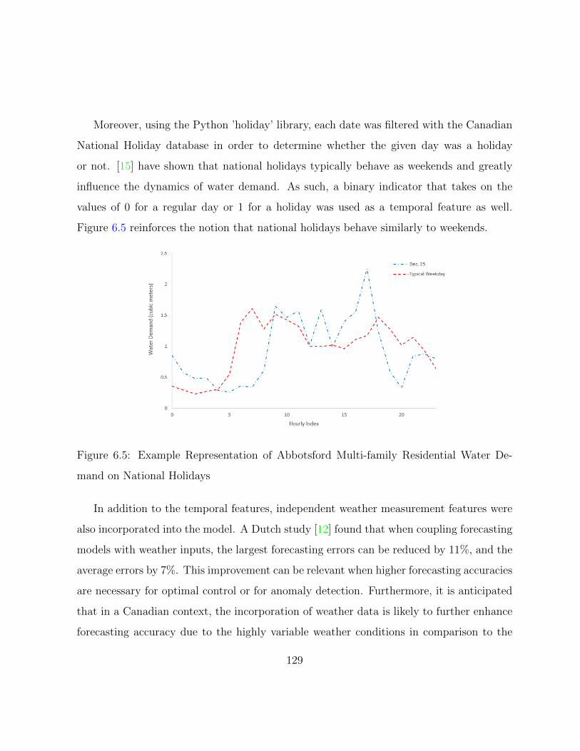
Moreover, using the Python ’holiday’ library, each date was filtered with the Canadian
National Holiday database in order to determine whether the given day was a holiday
or not. [15] have shown that national holidays typically behave as weekends and greatly
influence the dynamics of water demand. As such, a binary indicator that takes on the
values of 0 for a regular day or 1 for a holiday was used as a temporal feature as well.
Figure 6.5 reinforces the notion that national holidays behave similarly to weekends.
Figure 6.5: Example Representation of Abbotsford Multi-family Residential Water De-
mand on National Holidays
In addition to the temporal features, independent weather measurement features were
also incorporated into the model. A Dutch study [12] found that when coupling forecasting
models with weather inputs, the largest forecasting errors can be reduced by 11%, and the
average errors by 7%. This improvement can be relevant when higher forecasting accuracies
are necessary for optimal control or for anomaly detection. Furthermore, it is anticipated
that in a Canadian context, the incorporation of weather data is likely to further enhance
forecasting accuracy due to the highly variable weather conditions in comparison to the
129

moderate Dutch weather patterns. As such, hourly temperature measurements were incor-
porated. However, instead of using continuous or cumulative precipitation measurements
as a feature, a binary indicator was adopted instead. The binary indicator returns a value
of 0 or 1 if the current date is a clear day or foggy/rainy, respectively. The motivation for
this simplification was to mimic the approximate reasoning of human consumers, whereby
the average consumer is not concerned about the exact measurement of precipitation when
deciding to irrigate his/her lawn but rather uses intuition based on his/her own under-
standing of the probability of precipitation. Other factors such as wind velocity and air
pressure were deemed insignificant and were not included in the model.
Figure 6.6: Example Representation of Abbotsford Multi-family Residential Water De-
mand, Visual assessment of temperature influence
It can be observed in Figure 6.6 that additional demand occurs in the evening hours
during hot days. This is due to the additional sprinkler water consumption that occurs in
residential units during hot, summer days. Moreover, larger demands are seen during the
morning periods over a larger band, with the peak occurring earlier in the morning.
130

Lag features, time shifted values of the actual demand were also included in the model.
For example, lag 1 features will hold the demand value in the previous hour relative to
the current timestamp. In this model, lag features for the previous 6 hours (lags 1-6) were
utilized. In addition, lag features from the same hour during the previous day (lag-24)
and the previous week (lag-168) were added. The input database to the prediction engine
is assembled using the features as column fields whereby each observation is recorded as
a row. The target database will be composed of the hourly water demand consumed by
the city, reported in cubic meters per second (m3/s). The feature space of the predictive
model, excluding the lag terms, include:
• Xhour, a categorical discrete value representing the current hour of the day
• Xday, a categorical discrete value index representing the current day of the week
• Xmonth, a categorical discrete value index denoting the Month of the year
• Xholiday, a binary indicator whether day of the week is a national holiday
• Xtemp, a continuous value denoting the current ambient temperature (reported in
deg. Celsius)
• Xprecip- a binary indicator to denote whether current conditions are dry or rainy/cloudy
6.1.3 Results and Discussion
The MLP and ensemble tree regression models are quantitatively assessed using the three-
stage validation framework proposed in Chapter 5 and are evaluated using (1) a reduced
dataset (single MFRES meter); and (2) a larger dataset consisting of all residential meters
131

(over 23,000 SFRES and MFRES meters). In doing so, the generalization capacity of the
models are assessed at both the subdivision and city-level resolution. In each case, the error
model assumptions are tested by diagnostic metrics on the residuals, as well as by evaluat-
ing the predictive performance on independent validation sets. The structural validity of
the model is then assessed by performing a sensitivity analysis on the model’s features to
gauge their relative influence on the model’s predictive capacity. The model configurations
that were evaluated are summarized in Table 6.1. Note that hyper-parameter optimiza-
tion was conducted manually, using predominantly Scikit-learn’s (scikit-learn.org/) default
model settings.
Table 6.1: Model configurations for training and validation of estimators. MLP hidden
layer size is given by the total number of entries in {} where each entry denotes the
number of hidden neurons in that layer.
Model Model Architecture
MLP Hidden-layers: {15,12,10,9,8,7}; tanh
Random Forest 1000 estimators; default parameters
Bagging Trees 1000 estimators; default parameters
Boosted Trees 1000 estimators; default parameters
As part of the replicative validation phase, 10-fold cross validation was conducted to
assess the fidelity of the MLP model. The summary statistics (R2) from the cross-validation
testing of the single MLP estimator and ensemble decision tree models are shown in Table
6.2 for both the single meter and total residential meter datasets. At first glance, the
summary statistics of Table 6.2 suggest that the ensemble estimators, when compared to
the single estimator, exhibit less variance in their predictions, and are more robust in terms
132

of prediction errors in the testing sets. This appears to hold true at both scales of resolution.
However, using the suggested metrics as part of the replicative validation framework, the
reliability of these models can be further scrutinized. A preliminary analysis to compare
between the two model types is done at the single meter resolution since the potential
errors and biases are likely to be more pronounced, as suggested by Table 6.2.
Table 6.2: Confidence Intervals for Coefficient of Determination (R2) in validation datasets
Model R2 Single Meter R2 Total Residential (23,429 meters)
MLP 0.71 +/- 0.03 0.95 +/- 0.01
Random Forest 0.75 +/- 0.02 0.97 +/- 0.01
Boosted Trees 0.75 +/- 0.02 0.97 +/- 0.01
Bagging Trees 0.74 +/- 0.02 0.96 +/- 0.01
Figure 6.7 provides a visualization of the MLP estimator’s performance in terms of the
residuals’ ACF, histogram, Quantile-Quantile and regression plot of predictions versus ob-
servations. These visualizations are generated using the validation sets of the single meter
dataset. Similarly, Figure 6.8 provides the same level of visualizations for the Random
Forests. Since the Gradient Boosted Tree and Bagging Tree models performed similarly as
the Random Forests, their visualizations are omitted.
As shown in the ACF plot in Figure 6.7, the MLP model displays a trend in the
residuals, with statistically significant serial correlation evident in the 6th and 10th lag
components. This serial correlation is indicative of a deficiency in the model, potentially
attributed to the omission of important input information. The behavior of the residuals
can be further investigated via the provided histogram. While the shape of the histogram
of residuals is suggestive that the residuals are approximately normally distributed, the
133

Figure 6.7: Multilayer Perceptron Error Diagnostics: (a) Observed versus Predicted re-
gression plot (top left), (b) Residual histogram, (top right), (c) Residual ACF, (bottom
left) and (d) Quantile-Quantile plot of observed versus predicted measurements (bottom
right)
distribution is slightly offset from the standard normal distribution. This is typically in-
dicative that there is a slight bias in its predictive capacity. However, the residuals are
fairly tightly distributed about the mean. The Q-Q plot of the residuals and the regres-
sion plot of the predicted versus observed response variable both reinforce the previously
134

indicated model bias. It appears that the model is unable to reliably predict peak factors
in the demand signal, as shown by the significant deviation from the 1:1 line on both the
Q-Q and regression plots.
Figure 6.8: Random Forests Error Diagnostics: (a) Observed versus Predicted regression
plot (top left), (b) Residual histogram, (top right), (c) Residual ACF, (bottom left) and
(d) Quantile-Quantile plot of observed versus predicted measurements (bottom right)
Figure 6.8 highlights the performance of the Random Forest model. The models show
no trends in the ACF plot, and have no significant serial correlation. However, the residual
135

behaviour is similar to the MLP model, whereby a bias in the peak factors is evident.
Albeit, the bias is slightly less prominent in the ensemble models, in comparison with the
MLP model.
Figure 6.9: MLP Predicted versus Observed Demands: Validation Set Results
The predictive validity of the models is further investigated by assessing the perfor-
mance of each estimator against multiple independent test sets. A visual comparison of
each model is provided in Figures 6.9 - 6.10 for the MLP and ensemble models, respectively.
It is evident that in both cases, the models are able to capture the dynamics of the water
136

demand signal quite well. However, it is clear that the models are unable to effectively
capture the large peak signals, despite capturing the dynamics of the troughs in the model.
Figure 6.10: Random Forest Predicted versus Observed Demands: Validation Set Results
One of the reasons why the models are unable to capture the peaks effectively is because
of the high-resolution nature of the demand dataset. Since the models are being fit to the
observed water demand at a single metered location directly, the demand is more sensitive
to daily fluctuations in peak consumption. At the DMA level, these fluctuations would be
less pronounced and the model would be more equipped to capture the peak behavior. To
137

corroborate this hypothesis, the aforementioned validation metrics and visualizations are
applied to the total residential dataset, consisting of water demand measurements from
23,429 meters. Owing to its superior performance at the single meter resolution, the error
diagnostics and predictive performance in the validation set of the Random Forest model
is demonstrated in Figures 6.11 and 6.12, respectively.
The ACF plot in Figure 6.11 suggests that at the total residential scale, the Random
Forest model displays a slight trend in the residuals, with statistically significant serial
correlation evident in the 4th lag component. As suggested earlier, this serial correlation
is indicative of a slight deficiency in the model.However, the residuals are fairly tightly
distributed about the mean, as shown in the histogram, and follow the 1:1 line quite
closely in both the Q-Q and regression plots. This suggests that the previously indicated
model bias is substantially decreased at the total residential scale.
Figure 6.12 further reinforces the reduction in model bias when predicting at the total
residential scale. It is evident that the peaks and troughs are well characterized in the
predictions with no substantial errors.
Lastly,the Sobol sensitivity analysis was conducted to validate the structure of the pro-
posed models. In doing so, the relative importance of each feature in informing predictions
of the total residential water demand are assessed. As demonstrated in the barplot pro-
vided in Figure 6.13, the exogenous variables were not particularly important. In fact,
the results from the sensitivity indices seem to suggest that the following previous de-
mand measurements are most informative and are perhaps sufficient for building a robust
forecasting model:
• the previous two hours of demand, denoted by Lags ’1’ and ’2’
• the previous day’s demand at the same hour, denoted by Lag ’24’
138

Figure 6.11: Random Forests Error Diagnostics at the Total Residential Scale: (a) Ob-
served versus Predicted regression plot (top left), (b) Residual histogram, (top right), (c)
Residual ACF, (bottom left) and (d) Quantile-Quantile plot of observed versus predicted
measurements (bottom right)
• the previous week’s demand at the same hour, denoted by Lag ’168’
This strong dependency on previous measurements is undoubtedly an outcome of the
periodical behaviour of human water consumption. It suggests that in the absence of
139

Figure 6.12: Random Forest Predicted versus Observed Demands - Validation Set Results
at the Total Residential Scale
exogenous data, the model will still perform relatively well based on previous predictions
alone. Nonetheless, the proposed prediction engine will not preclude the use of exogenous
data since this information would be particularly useless for real-time management during
anomalous conditions.
It is difficult to compare the presented model’s performance with those presented in the
literature, since those models were fit to data at various data resolutions [4][124][56][154].
140

Figure 6.13: Sobol Sensitivity Indices produced via 7,000 iterations of the Random Forest
Prediction Model
In a study that uses a directly comparable performance metric [1], hourly R2 values of 0.792
and 0.896 (respectively) for their best ANN model configuration and wavelet-analysis ANN
were reported.Moreover, [4] reported RMSE values of 4.63 and 14.64 for their predictive
modelling during the training and validation phases, respectively. Similarly, [124] reported
Pearson Correlation coefficient (r) values of 0.73-0.92 during training and 0.55-0.91 during
testing for the various MLP-BP configurations that were tested. They also concluded
141

that their DAN2 model performed more consistently with r values ranging between 0.76-
0.88 during training and 0.85-0.91 during testing. Further, Herrera et al. reported MAE
and RMSE values of 3.02 and 4.33 for their best overall model. [56] found that when the
weekday and weekend models were combined, the training MAPE for this model was 2.08%
and the forecasting MAPE was 3.00%.
6.2 Case Study 2: Real-time Control and Optimiza-
tion
The City of Guelph, Ontario (Guelph) was selected as a pilot project for the implemen-
tation and evaluation of this novel RTC platform. Guelph is located in the Grand River
Watershed, which is part of the Lake Erie Source Protection Region, and services a popu-
lation of approximately 125,000 consumers. Guelph is also one of the largest municipalities
in Canada to rely almost exclusively on groundwater for its drinking water supply (City of
Guelph Water Supply Master Plan, 2006). Guelph’s water supply and distribution system
consists of 570 kilometers of water mains ranging in diameter from 100 mm to 900 mm,
five underground storage reservoirs with a combined capacity of 48,000 cubic meters, three
elevated water storage towers and 22 pumping stations (City of Guelph Water Supply
Master Plan, 2006).
The City’s hydraulic model was previously calibrated and updated in 2011 and in-
cluded a complete update of all pump curves, reservoirs, elevated tanks and demands. The
2012 demands for an average and a maximum demand day were added to the model and
calibrated accordingly. This model was utilized as the starting point for this project.
142

Figure 6.14: City of Guelph Water Supply System Map (City of Guelph Water Supply
Master Plan, 2006)
143

6.2.1 Input Datasets
The Guelph pumping systems consist entirely of constant-speed pumps (CSP). As such
the input datasets of interest to be incorporated in the model include Pump Performance
and Efficiency Curves.
The City completed a number of field tests to verify the operating pump curves of
each pumping system. This data encapsulates the head-flow relationships of each pumping
system and defines its hydraulic performance over a wide range of operating conditions.
Moreover, in order to calculate the amount of energy consumed by each pump, efficiency
curves were added to the model. The City provided manufacturers’ data sheets. Only the
most updated datasets were incorporated in order to keep the model parsimonious.
Guelph Hydro charges the City at four different rate structures depending on the size
and type of the service. These rate structures were incorporated as inputs to the hydraulic
model:
1. Service Size 1, Monthly load demand less than 50 kW:
(a) regulated Price Plan (RPP) Time-of-Use Pricing, the consumption in kilowatt
hours is separated into three periods: on-peak, mid-peak and off-peak, with a
different cost rate for each period; and
(b) RPP Two-Tiered Pricing, the consumption in kilowatt hours (kWh) is separated
into two price tiers under the government’s Regulated Price Plan with the price
threshold being 750 kWh based on a 30-day billing period. As the threshold
is typically exceeded within the initial 24 hours of operation during a monthly
billing period the upper threshold (greater than 750 kWh) is utilized in model.
2. Service Size 2, Monthly load demand between 50 and 999 kW:
144

(a) weighted Average Hourly Spot Market Price (WAHSP), the Weighted Average
Hourly Spot Price (WAHSP) is applied to non-RPP and non-retail customers,
without interval metering; and
(b) hourly Ontario Energy Price, interval-metered customers are billed at the Hourly
Ontario Energy Price (HOEP).
Water demand information was incorporated in the model to reflect the standard op-
erational scenario archetypes, namely a Typical Day. The Typical Day was chosen as
October 3, 2012 with a demand of 44 ML/d.
6.2.2 Boundary Conditions and Operational Constraints
In order to establish initial and bounding conditions for the optimization strategy, state
variables were monitored in real-time via outputs from the hydraulic model and were
subsequently evaluated against operational constraints. Pump schedules that produced
operational constraint violations were demarcated as infeasible and were not recommended
as part of the optimization strategy. Initial conditions are set at the beginning of each
timestep using SCADA measurements of the state variables. In lieu of such measurements,
the simulation output from the previous timestep is used.
As detailed in Chapter 3, constraints were set on system pressure and storage. Terminal
constraints to ensure the stability of the controller were also imposed on the storage tanks
and reservoirs. Table 6.3 summarises the operational constraints that have been imposed
onto each state variable.
In order to improve model response time a subset of representative monitoring junctions
was selected to assess the feasibility of system pressures. These monitoring junctions
145
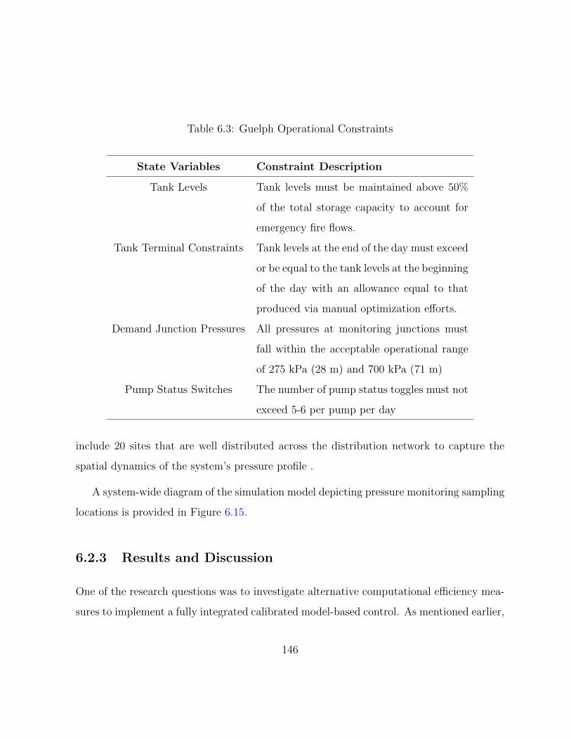
Table 6.3: Guelph Operational Constraints
State Variables Constraint Description
Tank Levels Tank levels must be maintained above 50%
of the total storage capacity to account for
emergency fire flows.
Tank Terminal Constraints Tank levels at the end of the day must exceed
or be equal to the tank levels at the beginning
of the day with an allowance equal to that
produced via manual optimization efforts.
Demand Junction Pressures All pressures at monitoring junctions must
fall within the acceptable operational range
of 275 kPa (28 m) and 700 kPa (71 m)
Pump Status Switches The number of pump status toggles must not
exceed 5-6 per pump per day
include 20 sites that are well distributed across the distribution network to capture the
spatial dynamics of the system’s pressure profile .
A system-wide diagram of the simulation model depicting pressure monitoring sampling
locations is provided in Figure 6.15.
6.2.3 Results and Discussion
One of the research questions was to investigate alternative computational efficiency mea-
sures to implement a fully integrated calibrated model-based control. As mentioned earlier,
146

Figure 6.15: Model output of pressure monitoring junctions. The high-pressure belt is
delimited with a black rectangle.
integrating a full hydraulic model into the RTC platform allows for a more comprehen-
sive evaluation of the current and projected behaviour of the WSD, thus empowering the
operational staff to render decisions based on a holistic a priori understanding of system
performance.
The first step involved simply processing the EPANET2 model input file and stripping
any extraneous content. While this process was laborious, the simulation model runtime
was reduced by over an order of magnitude, from 30 seconds to 3 seconds. Furthermore,
147

by reducing the amount of network information that was stored in memory, and efficiently
handling input and output hydraulic data throughout the platform at every model evalu-
ation, the runtime per simulation was further reduced to 1.8 seconds.
However, the primary computational efficiency measure involved parallelizing the RT-
DDS framework for distributed and shared memory computing architectures, namely through
the implementation of MPI-based communications. While on average, computational bud-
gets of 500 and 1,000 iterations were sufficient in converging to what appeared to be
near-optimal solutions (true optimal is unknown), these budgets still resulted in an aver-
age reporting frequency of 15-30 mins. The reporting frequency is critical since operators
require time to consider implementing the optimized pump schedule for the next hour.
This is still a considerable achievement when using a fully calibrated hydraulic model, but
further computational efficiencies could be achieved via parallelization. When using the
MPI formulation of RT-DDS on a local server, the reporting frequency at each timestep
could be reduced to 10 minutes with 1,000 iterations. Alternatively, the optimizer could
be executed with many more iterations. A 10-minute reporting frequency is on-par with
those reported by [145] when using a surrogate ANN model.
The second set of numerical experiments that was conducted with the City of Guelph
RTC case study involved evaluating the relative performance of each control variable for-
mulation, namely the TCT and BSC representations. Specifically, the relative performance
of each control variable is assessed based on its influence on the convergence quality of op-
timization search trajectory at each timestep, the computational efficiency of execution
across various computational scales, as well as the observable variability of recommended
pump schedules.
Figure 6.16 shows the convergence behaviour of both the BSC and TCT formulations on
a representative control timestep (hour 0). In this experiment, both representations were
148

Figure 6.16: Convergence Profile of serial TCT and serial BSC on representative control
timestep, 1000 function evaluations (run-time of less than 2,000 seconds). Both TCT and
BSC were initialized with the same warm start solution in two unique experiments (1,2).
initialized with the same warm solution and were provided the same computational budget.
It is clearly observable that the TCT formulation is able to rapidly converge to the feasible
region of the decision space, as well as achieve near-optimal results within a fraction of
the computational budget. In fact, Figure 6.16 demonstrates that the TCT formulation is
able to achieve superior decision schedules than the manual recommendations within 1/8th
of the required budget. This suggests that the TCT formulation can produce superior
schedules than a human-optimized schedule within 5 minutes of computational time, or
1.5 minutes when parallelized across a typical desktop computer’s processing cores.
Figure 6.16 further suggests that the TCT formulation can perform robustly within a
10-minute reporting frequency without the need to substitute a full hydraulic model with a
149

surrogate representation. On the other hand, it is evident that binary representation faces
challenges with breaking out of the infeasible region of the decision space throughout the
search trajectory. The demonstrated convergence ultimately reinforces the computational
limitation of the BSC formulation, whereby the decision space for the same TCT schedule
is orders of magnitude larger, as demonstrated in Chapter 3. While this limitation can
be addressed by feeding the BSC formulation with a feasible, near-optimal warm solution,
this requirement renders this formulation undesirable for emergency scenarios, where rapid
adaptation is required and no previously known feasible or optimal solutions exist.
However, it should be noted that the BSC formulation, shown in Appendix B, produces
recommended schedules that are far more uniform than those produced by the TCT formu-
lation, also shown in Appendix B. Independent tests were run with the same computational
budget and warm start solution to see how the recommended optimal schedules produced
by each formulation vary from one another. The goal of this experiment was to gauge how
each formulation’s recommendations would vary on a daily basis under standard operat-
ing conditions, whereby little deviations in demand are observed. In idealized scenario,
the optimizer would converge to similar recommended decision schedules when fed with
the same warm solution, computational budget and disturbance profile. This would be
attractive for operational staff who would ideally not like to change their modus operandi
significantly on a daily basis.
Unsurprisingly, Appendix B reveals that the BSC formulation results in recommended
schedules that vary insignificantly in comparison with the TCT formulation. This is be-
cause the large discrete decision space results in changes that are sparsely distributed across
multiple pumps and control horizon whereas perturbations in the tighter decision space of
the TCT formulation result in larger changes in the schedule.
In assessing the BSC and TCT performance results on a typical day, it was found
150

that both formulations significantly outperformed the manual and baseline operations. As
demonstrated in Figure ??, both the BSC and TCT formulations yielded maximimum
energy cost savings of 26% and 31%, respectively, relative to baseline operations. This
translated to per annum savings of $247,547 and $293,807, or $7.2/ML or $8.4/ML of
production flow, respectively.
However, as predicted, it should be noted that in a few occasions both the TCT and BSC
formulations resulted in schedules that violated the maximum permissible pump switches.
These violations can be observed in Appendix A. Given the favourable convergence per-
formance of the TCT representation and a need to address the potential for pump switch
violations, the performance of the F-TCT formulation was further investigated.
Figure 6.17: Convergence Profile of F-TCT on representative control timestep, 1000 func-
tion evaluations (run-time of less than 2,000 seconds)
151

As demonstrated in Figure 6.17, the F-TCT formulation exhibits a similar convergence
profile as the original TCT formulation. This is particularly attractive given that every
timestep the F-TCT formulation is solving a more constrained problem than the TCT
counterpart. In this manner, the F-TCT guarantees that no pump switch violations are
incurred over the duration of any calendar day (also detailed in Appendix A).
Figure 6.18: Average Energy Savings of F-TCT Real-time Controller relative to Manual
and Baseline Operations
A summary of the total energy savings produced by the F-TCT driven real-time con-
troller is presented in Figure 6.18. As observed, a maximum savings of 25% (24.5% on
average) can be achieved via the optimized strategy for the Typical day scenario. The
energy savings were benchmarked relative to Guelph’s baseline operations as well as the
consultant’s manual optimized recommendations (as part of SWI project). While the an-
ticipated total energy savings are less than those initially produced by the TCT (31%)
and binary (26%) formulations, the F-TCT formulation is more robust since it guarantees
152

that at any arbitrary calendar date the operational limits on pump switches are never
exceeded. In this manner, the F-TCT formulation is likely to create more desired system
hydraulic behavior. The distribution of energy cost savings results obtained from repeated
experiments with each control variable formulation is detailed in Figure 6.19.
Figure 6.19: Boxplot of Normalized Energy Savings for each Control Variable Formulation,
BSC, TCT and F-TCT. 3 experiments were conducted for BSC and F-TCT, and 7 were
conducted for TCT.
However, it should be noted that Figures 6.18 and 6.19 reveal that the F-TCT formula-
tion performs well relative to manual operations with the assumption of perfect knowledge
of the system demand profile. As such, further investigation is required to assess its per-
formance when demands are forecasted in real-time. While insufficient data was provided
to be able to train a prediction engine for forecasting demand in the City of Guelph,
the behaviour of a prediction engine was simulated by introducing Gaussian noise to the
known forecasts. In doing so, the demand profile at every control timestep is disturbed
153

in a manner similar to the errors produced by a prediction model. The introduction of
Gaussian noise to the forecasts is assumed to be a valid approach given that the distribu-
tion of the forecasting error residuals in Chapter 6.2 are normally distributed. Example
noise-perturbed demand profiles are provided in Figure 6.20.
Figure 6.20: Typical Day Demand Profile Perturbed with Gaussian Noise. 1000 simulated
profiles are shown against the known typical day demand (in black).
At every control timestep, a new noise-perturbed demand profile was generated based
on the known noise-free profile at that time. This was done to simulate the self-correcting
behaviour of the prediction engine in real-time whereby the actual known demand observa-
tions from SCADA are used to initialize the demand predictions at every timestep. When
evaluating the F-TCT formulation with the noise-perturbed demand profile, it was found
that the algorithm still maintained hydraulic feasibility and generated energy cost savings
that were in the same range (21%) as those produced with the perfect demand assumption.
154

The cost savings were evaluated by evaluating the recommended pump schedule (produced
with the noise-perturbed demands) at the end of the day with the known demands. This
demonstrates that the control formulation is adaptive to changes in the demand profile.
Figure 6.21: Averaged Pressure head profile of F-TCT driven RT-DDS
The state variable outputs, namely pressure and tank levels, for the F-TCT driven
platform were assessed in detail as part of the analysis, and are summarized via Figures
6.21-6.22 for visualization.
The observed pressures for each zone are averaged across all monitoring nodes and
visualized in Figure 6.21. It is immediately evident that under the real-time optimized
scenarios, pressure head levels across each zone change very little from existing conditions.
Moreover, the pressures within each zone are tightly coupled with no significant changes
in both morning and evening peak demand hours. This is particularly attractive from an
155

Figure 6.22: Elevated Storage Tank Levels produced by F-TCT driven RT-DDS
operational perspective, whereby significant changes in pressure within a typical day are
undesirable.
As detailed in Figure 6.22, the elevated storage tank levels vary within a fairly tight
operational band (30% of capacity). This band is desirable for maintaining emergency
storage volumes in the system. RT-DDS further ensures that the tanks do not lose stability
over the day by ensuring the terminal constraints are satisfied. As observed, all tanks are
nearly full right before both morning and evening peak hours, and then experience a decline
as pumps are shut-off as part of the optimization process. The Speedvale tank experiences
the sharpest decline after the morning peak demand.
Detailed information on pump key performance indicators (KPIs) can be instrumental
for operators to assess how their assets are performing in real-time. As such, plots of the
156

Figure 6.23: Contribution of each Pumping System to overall cost
system pump KPIs are provided in Figures 6.23 - 6.24. Included are the projected daily
cost contributions of each pumping system, the energy intensity (kWh/m3) and pump
utilization rates (%), and lastly the pumping system average and peak energy consump-
tions. These plots enable an operator to proactively assess how efficiently each pump is
operating and the average consumption, utilization and costs attributed to each pump in
the system. These plots could be used to reinforce or contradict the operator’s judgement
on which pumps should be scheduled most frequently. As observed in Figure 6.23, the
largest cost contributor to the total system costs is the Woods pumping station, largely
due to its rated capacity. However, as shown in Figure 6.24, the Woods system is actually
relatively efficient. For this reason, the Woods system is fairly well utilized by the RT-DDS
platform. Other large cost contributors include the Arkell, Park St.,Downey and Emma
157

Figure 6.24: Energy Intensity versus Utilization Rates for each pumping system
well systems.
It can also be generally observed that the RT-DDS algorithm intelligently schedules
pumps such that pumps with the highest efficiencies (lower energy intensity) are utilized
the most (as demonstrated by the utilization versus energy intensity plot provided in
Figure 6.24). For example, the Calico and Helmar pumping systems suffer from relatively
high energy intensity rates (KWh/m3), yet have utilization rates below 15%. Conversely,
pumps with relatively low energy intensity rates (KWh/m3), such as Robertson, Arkell,
Paisley and Woods, were utilized the most. It should be noted that the Emma well pump
seems to be the exception to this case. However, the Emma pump system was not a control
variable and was thus responding to the system hydraulic conditions based on it’s existing
tank setpoints.
158

Long-term potential cost savings that can be achieved through the use of the RT-DDS
platform were also projected. The projection assumes that the platform is able to gener-
ate cost savings consistently each year over its lifetime, with no substantial degradation
in performance. The 10-year projected savings was computed ignoring the influence of
annualized growth, inflation and interest rates, in order to provide a lower bound estimate
of potential long term savings.
Table 6.4: Long-term Cost Savings of Real-time Controller
RT-DDS Savings
Estimated Annual Cost $951,519
Percentage Savings 25%
Annual Cost Savings $233,589
Savings over Lifetime $2,335,891
As demonstrated in Table 6.4, the long term cost savings are substantial. Note that
these savings scale proportionally to the size and complexity of the distribution system
under analysis. As such, integrating an RTC platform with WSDs across the province could
yield significant savings in terms of both annualized costs and Greenhouse Gas emissions.
159

Chapter 7
Concluding Remarks
In this research, a novel predictive real-time control and optimization platform, RT-DDS,
is introduced and quantitatively assessed. The platform is designed to provide real-time
pump control setting recommendations in the form of a 24-hour schedule based on current
system conditions and is thus able to dynamically adjust to changes in the system. The
RT-DDS platform was configured to solve an optimization problem at every timestep in
the control horizon (24-hours) through the minimization of energy costs while maintaining
system behaviour within a predefined regulatory and operational tolerance band.
In doing so, multiple control variable formulations were assessed. These included binary
control statuses and time-controlled triggers whereby the pump schedule was represented
as a sequence of on/off binary variables and active/idle discrete time zones, respectively.
However, it was found that both formulations led to conditions whereby the system would
violate the predefined maximum number of pump switches per calendar day. This occurred
at each timestep because the control variable formulation was unaware of the elapsed
switches in the subsequent hours. As such, a novel feedback architecture was proposed,
160

such that at every timestep, the number of switches that had elapsed in the previous hours
was explicitly encoded into the formulation. In this manner, the maximum number of
switches per calendar day was never violated. Using this novel formulation, daily energy
cost savings of up to 25% were achievable on an average day, which translated to savings of
over 2.3 million dollars over a ten year period. Moreover, stable hydraulic conditions were
produced in the system, thereby changing very little when compared to baseline operations
in terms of quality of service and overall condition of assets.
The prediction engine of the RT-DDS platform was evaluated with an AMI-driven case
study, whereby the water consumption of the residential units in the city were predicted. A
Multi-Layer Perceptron (MLP) and ensemble-driven learning techniques (Random forests,
Bagging trees and Boosted trees) were all built, trained and validated as part of this re-
search. A three-stage validation process was adopted to assess the replicative, predictive
and structural validity of the models. The models were tested at two resolutions to assess
the generalization capacity of the models at predicting water demand at a single meter, and
then at the city-scale, by predicting the total residential demand. While the models proved
to have strong generalization capability, via good performance in the cross-validation test-
ing, all models experienced slight biases when aiming to predict extreme peak events in
the single meter dataset. It was concluded that the models performed far better at the
city resolution whereby peak events are far more normalized. Moreover, the relative influ-
ence of exogenous parameters was assessed via a global sensitivity analysis. In doing so, it
was found that a sufficiently robust model could be constructed using historical demand
measurements alone. In general, the models demonstrated the capacity of using machine
learning techniques in for short term water demand forecasting particularly in the context
of real-time control and optimization.
The following research recommendations are made to further enhance the performance
161

of the proposed RT-DDS platform:
• it is recommended that a multi-objective optimization problem is formulated to assess
how well the real-time platform can negotiate the trade-off between reliability of
supply and minimization of costs;
• the resilience of the RT-DDS platform ought to be further investigated by testing the
platform with several emergency conditions such as blackouts and fire flows;
• it is recommended that high-resolution surrogate models of the water supply and
distribution infrastructure are explored in order to enhance the robustness of the
RT-DDS platform;
• the platform can be integrated with water quality data to assess how well water
quality objectives such as water age minimization and chlorine residual stabilization
can be adapted into the framework; and
• from an algorithmic optimization perspective, it is recommended that various search
heuristics be further explored to assess whether preferential activation of pumps based
on efficiency and capacity can enhance overall system performance.
162

References
[1] Adamowski, J., Chan, H. F., Prasher, S. O., Ozga-Zielinski, B., and
Sliusarieva, A. Comparison of multiple linear and nonlinear regression, autore-
gressive integrated moving average, artificial neural network, and wavelet artificial
neural network methods for urban water demand forecasting in montreal, canada.
Water Resources Research 48, 1 (2012).
[2] Alba, E., Luque, G., and Nesmachnow, S. Parallel metaheuristics: recent
advances and new trends. International Transactions in Operational Research 20, 1
(2013), 1–48.
[3] Alba, E., Nakib, A., and Siarry, P. Metaheuristics for Dynamic Optimization,
1 ed., vol. 433 of 10. Springer, Berlin Heidelberg, 2013.
[4] Alvisi, S., Franchini, M., and Marinelli, A. A short-term, pattern-based
model for water-demand forecasting. Journal of Hydroinformatics 9, 1 (2007), 39–
50.
[5] Anderson, R. L., Miller, T. A., and Washburn, M. C. Water savings from
lawn watering restrictions during a drought year, fort collins, colorado. JAWRA
Journal of the American Water Resources Association 16, 4 (1980), 642–645.
163

[6] Anzaldi, G., Rubion, E., Corchero, A., Sanfeliu, R., Domingo, X., Pi-
juan, J., and Tersa, F. Towards an enhanced knowledge-based decision support
system (dss) for integrated water resource management (iwrm). Procedia Engineering
89 (2014), 1097–1104.
[7] Arrondo, A., Redondo, J., Fernandez, J., and Ortigosa, P. M. Paral-
lelization of a non-linear multi-objective optimization algorithm: Application to a
location problem. Applied Mathematics and Computation 255 (3/15 2015), 114–124.
[8] Asadzadeh, M., Razavi, S., Tolson, B. A., and Fay, D. Pre-emption strate-
gies for efficient multi-objective optimization: Application to the development of lake
superior regulation plan. Environmental Modelling Software 54 (4 2014), 128–141.
[9] Asadzadeh, M., Tolson, B. A., and Burn, D. H. A new selection metric for
multiobjective hydrologic model calibration. Water Resources Research 50, 9 (2014),
7082–7099.
[10] Athanasiou, S., Staake, T., Stiefmeier, T., Sartorius, C., Tompkins, J.,
and Lytras, E. Daiad: Open water monitoring. Procedia Engineering 89 (2014),
1044–1049.
[11] Bai, Y., Wang, P., Li, C., Xie, J., and Wang, Y. A multi-scale relevance
vector regression approach for daily urban water demand forecasting. Journal of
Hydrology 517 (9/19 2014), 236–245.
[12] Bakker, M., van Duist, H., van Schagen, K., Vreeburg, J., and Ri-
etveld, L. Improving the performance of water demand forecasting models by
using weather input. Procedia Engineering 70, Complete (2014), 93–102.
164
[13] Bakker, M., van Schagen, K., and Timmer, J. Flow control by prediction
of water demand. Journal of Water Supply: Research and Technology - Aqua 52, 6
(09/01 2003), 417–424.
[14] Bakker, M., Vreeburg, J. H. G., Palmen, L. J., Sperber, V., Bakker, G.,
and Rietveld, L. C. Better water quality and higher energy efficiency by using
model predictive flow control at water supply systems. Journal of Water Supply:
Research and Technology - Aqua 62, 1 (02/01 2013), 1–13.
[15] Bakker, M., Vreeburg, J. H. G., van Schagen, K. M., and Rietveld,
L. C. A fully adaptive forecasting model for short-term drinking water demand.
Environmental Modelling Software 48 (10 2013), 141–151.
[16] Baran, B., von Lucken, C., and Sotelo, A. Multi-objective pump scheduling
optimisation using evolutionary strategies. Advances in Engineering Software 36, 1
(2005), 39 – 47.
[17] Barham, R. H., and Drane, W. An algorithm for least squares estimation of
nonlinear parameters when some of the parameters are linear. Technometrics 14, 3
(1972), 757–766.
[18] Berardi, L., Giustolisi, O., and Todini, E. Enhanced global gradient algo-
rithm: A general formulation. In Proceedings of World Environmental and Water Re-
sources Congress 2009 - World Environmental and Water Resources Congress 2009:
Great Rivers (2009), vol. 342, pp. 209–218.
[19] Bishop, C. M. Neural Networks for Pattern Recognition. Oxford University Press,
Inc., New York, NY, USA, 1995.
165

[20] Boccelli, D. L. Optimal scheduling of booster disinfection in water distribution
systems. J. Water Resour. Plann. Manage. 124 (1998), 99.
[21] Bougadis, J., Adamowski, K., and Diduch, R. Short-term municipal water
demand forecasting. Hydrological Processes 19, 1 (2005), 137–148.
[22] Boulos, P., Wu, Z., Orr, C., Moore, M., Hsuing, P., and Thomas, D.
Optimal pump operation of water distribution systems using genetic algorithms.
In American Water Works Association Distribution System Symposium (Denver,
Colorado, 2001).
[23] Bounds, P. Efficient energy management of a large-scale water supply system. Civ.
Eng. Environ. Syst. 23 (2006), 209.
[24] Bowden, G. J. Optimal division of data for neural network models in water re-
sources applications. Water Resour. Res. 38 (2002), 1010.
[25] B.Paechter, Lopez-Ibanez, M., and Prasad, T. D. Ant-Colony Optimization
for Optimal Pump Scheduling.
[26] Braun, M., Bernard, T., Piller, O., and Sedehizade, F. 24-hours demand
forecasting based on sarima and support vector machines. Procedia Engineering 89
(2014), 926–933.
[27] Breiman, L. Bagging predictors. Machine Learning 24, 2 (1996), 123–140.
[28] Breiman, L. Random forests. Machine Learning 45, 1 (2001), 5–32.
[29] Broad, D. R. Water distribution system optimization using metamodels. J. Water
Resour. Plann. Manage. 131 (2005), 172.
166

[30] Bunn, S. Closing the loop in water supply optimisation. In 2007 IET Water Event
(2007), pp. 71–82.
[31] Candelieri, A., and Archetti, F. Identifying typical urban water demand
patterns for a reliable short-term forecasting the icewater project approach. Procedia
Engineering 89 (2014), 1004–1012.
[32] Candelieri, A., Soldi, D., and Archetti, F. Short-term forecasting of hourly
water consumption by using automatic metering readers data. Procedia Engineering
119 (2015), 844–853.
[33] Carbone, M., Garofalo, G., and Piro, P. Decentralized real time control
in combined sewer system by using smart objects. Procedia Engineering 89 (2014),
473–478.
[34] Chen, J., and Boccelli, D. L. Demand forecasting for water distribution sys-
tems. Procedia Engineering 70 (2014), 339–342.
[35] Cheng, W. P., Yu, T. C., and Xu, G. Real-time model of a large-scale water
distribution system. Procedia Engineering 89 (2014), 457–466.
[36] Chorley, M., and Walker, D. Performance analysis of a hybrid mpi/openmp
application on multi-core clusters. Journal of Computational Science 1, 3 (8 2010),
168–174.
[37] Confesor, R., and Whittaker, G. Automatic calibration of hydrologic mod-
els with multi-objective evolutionary algorithm and pareto optimization1. JAWRA
Journal of the American Water Resources Association 43, 4 (2007), 981–989.
167

[38] Coulbeck, B., Brdys, M., Orr, C. H., and Rance, J. P. A hierarchical
approach to optimized control of water distribution systems: Part i decomposition.
Optimal Control Applications and Methods 9, 1 (1988), 51–61.
[39] Coulbeck, B., Brdys, M., Orr, C. H., and Rance, J. P. A hierarchical
approach to optimized control of water distribution systems: Part ii. lower-level
algorithm. Optimal Control Applications and Methods 9, 2 (1988), 109–126.
[40] Dandy, G. C., Maier, H. R., and Broad, D. R. Optimal operation of complex
water distribution systems using metamodels. Journal of Water Resources Planning
and Management 136, 4 (2010), 433–443.
[41] Deb, K. An efficient constraint handling method for genetic algorithms. Computer
Methods in Applied Mechanics and Engineering 186, 24 (6/9 2000), 311–338.
[42] Deb, K., Pratap, A., Agarwal, S., and Meyarivan, T. A fast and elitist
multiobjective genetic algorithm: Nsga-ii. Evolutionary Computation, IEEE Trans-
actions on 6, 2 (2002), 182–197.
[43] Deuerlein, J. W. Decomposition model of a general water supply network graph.
J. Hydraul. Eng. 134 (2008), 822.
[44] Diehl, M., Ferreau, H. J., and Haverbeke, N. Efficient Numerical Methods
for Nonlinear MPC and Moving Horizon Estimation. Springer Berlin Heidelberg,
Berlin, Heidelberg, 2009, pp. 391–417.
[45] Donkor, E., Mazzuchi, T., Soyer, R., and Roberson, J. A. Urban water
demand forecasting: Review of methods and models. Journal of Water Resources
Planning and Management 140, 2 (02/01; 2015/11 2014), 146–159.
168

[46] Drucker, H. Improving regressors using boosting techniques. In Proceedings of
the Fourteenth International Conference on Machine Learning (San Francisco, CA,
USA, 1997), ICML ’97, Morgan Kaufmann Publishers Inc., pp. 107–115.
[47] Drucker, H., Schapire, R. E., and Simard, P. Improving performance in
neural networks using a boosting algorithm. In Advances in Neural Information
Processing Systems 5, [NIPS Conference] (San Francisco, CA, USA, 1993), Morgan
Kaufmann Publishers Inc., pp. 42–49.
[48] Ercan, M. B., Goodall, J. L., Castronova, A. M., Humphrey, M., and
Beekwilder, N. Calibration of swat models using the cloud. Environmental Mod-
elling Software 62 (12 2014), 188–196.
[49] Espinoza, F. P. Effects of local search algorithms on groundwater remediation
optimization using a self-adaptive hybrid genetic algorithm. J. Comput. Civ. Eng.
20 (2006), 420.
[50] Filion, Y., MacLeod, S., and Roshani, E. Evaluating the impact of climate
change mitigation strategies on the optimal design and expansion of the amherstview,
ontario, water network: Canadian case study. Journal of Water Resources Planning
and Management 138, 2 (2012), 100–110.
[51] Fontenot, E., Ingeduld, P., and Wood, D. Real Time Analysis of Water
Supply and Water Distribution Systems. American Society of Civil Engineers, 06/17;
2015/11 2003, pp. 1–10.
[52] Freund, Y., and Schapire, R. A decision theoretic generalization of on-line
learning and an application to boosting, 2010.
169

[53] Gage, G., Helmcke, S., and Prigent, O. The 21st century water utility ini-
tiative: How to boost operational performance of water utilities by up to 20 Water
Science and Technology 68, 7 (2013), 1487–1494.
[54] Ganidi, N., and Holden, B. Real time control of water distribution systems using
a multi-criteria decision-support tool for optimal water network management a case
study. Procedia Engineering 89 (2014), 495–501.
[55] Garrick, N., and Felder, M. Water and the future of the canadian economy
report. Tech. rep., The Innovolve Group, 294 Richmond Street East, Suite 200,
Toronto, Ontario, 2010.
[56] Ghiassi, M., Zimbra, D., and Saidane, H. Urban water demand forecasting
with a dynamic artificial neural network model. Journal of Water Resources Planning
and Management 134, 2 (03/01; 2015/11 2008), 138–146.
[57] Ghiassi, M., Zimbra, D. K., and Saidane, H. Medium term system load
forecasting with a dynamic artificial neural network model. Electric Power Systems
Research 76, 5 (2006), 302 – 316.
[58] Giacomello, C., Kapelan, Z., and Nicolini, M. Fast hybrid optimization
method for effective pump scheduling. Journal of Water Resources Planning and
Management 139, 2 (03/01; 2016/11 2013), 175–183.
[59] Goldberg, D. Genetic Algorithms in Search, Optimization and Machine Learning,
1st ed. Addison-Wesley Longman Publishing Co., Inc., Boston, MA, USA, 1989.
[60] Goldman, F., and Mays, L. The application of simulated annealing to the optimal
operation of water systems. American Society of Civil Engineers (ASCE), 1999.
170

[61] Hadka, D., Madduri, K., and Reed, P. Scalability analysis of the asynchronous,
master-slave borg multiobjective evolutionary algorithm. In Parallel and Distributed
Processing Symposium Workshops PhD Forum (IPDPSW), 2013 IEEE 27th Inter-
national (2013), pp. 425–434.
[62] Hadka, D., and Reed, P. Large-scale parallelization of the borg multiobjec-
tive evolutionary algorithm to enhance the management of complex environmental
systems. Environmental Modelling Software 69 (7 2015), 353–369.
[63] Hagan, M. T., and Menhaj, M. B. Training feedforward networks with the
marquardt algorithm. IEEE Transactions on Neural Networks 5, 6 (1994), 989–993.
[64] Hansen, L. K., and Salamon, P. Neural network ensembles. Pattern Analysis
and Machine Intelligence, IEEE Transactions on 12, 10 (1990), 993–1001.
[65] Harou, J. J., Garrone, P., Rizzoli, A. E., Maziotis, A., Castelletti, A.,
Fraternali, P., Novak, J., Wissmann-Alves, R., and Ceschi, P. A. Smart
metering, water pricing and social media to stimulate residential water efficiency:
Opportunities for the smarth2o project. Procedia Engineering 89 (2014), 1037–1043.
[66] Herrera, M., Torgo, L., Izquierdo, J., and Perez-Garcia, R. Predictive
models for forecasting hourly urban water demand. Journal of Hydrology 387, 12
(6/7 2010), 141–150.
[67] Hughes, T. C. Peak period design standards for small western u.s. water supply
systems1. JAWRA Journal of the American Water Resources Association 16, 4
(1980), 661–667.
171

[68] Humphrey, G., Maier, H., Wu, W., Mount, N., Dandy, G., Abrahart,
R., and Dawson, C. Improved validation framework and r-package for artificial
neural network models. Environmental Modelling Software 92 (6 2017), 82–106.
[69] Hutton, C., Kapelan, Z., Vamvakeridou-Lyroudia, L., and Savi, D. Deal-
ing with uncertainty in water distribution system models: A framework for real-time
modeling and data assimilation. Journal of Water Resources Planning and Manage-
ment 140, 2 (02/01; 2015/11 2014), 169–183.
[70] Huzmezan, M., and Maciejowski, J. M. Reconfigurable flight control of a
high incidence research model using predictive control. In Control ’98. UKACC
International Conference on (Conf. Publ. No. 455) (1998), pp. 1169–1174 vol.2.
[71] Irons, L., Boxall, J., Speight, V., Holden, B., and Tam, B. Data driven
analysis of customer flow meter data. Procedia Engineering 119 (2015), 834–843.
[72] Ivetic, D., Vasilic, Z., Prodanovic, D., and Stanic, M. Implementing q
method to accelerate the optimization of pressurized pipe networks. Procedia Engi-
neering 89 (2014), 618–625.
[73] Jain, A., Kumar Varshney, A., and Chandra Joshi, U. Short-term water
demand forecast modelling at iit kanpur using artificial neural networks. Water
Resources Management 15, 5 (2001), 299–321.
[74] Jain, A., and Ormsbee, E. L. Short-term water demand forecast modeling
techniques-conventional methods versus artificial intelligence. Journal (American
Water Works Association) 94, 7 (2002), 64–72.
172

[75] Jamieson, D., Shamir, U., Martinez, F., and Franchini, M. Conceptual
design of a generic, real-time, near-optimal control system for water-distribution
networks. Journal of Hydroinformatics 9, 1 (Portland Press Ltd 2007), 3–14.
[76] Jank, B. Instrumentation, control and automation of water and wastewater treat-
ment and transport systems 1993. Water Science Technology 28, 11-12 (1993).
[77] Jayasekara, P., Illangasinghe, D., Dahanayake, J., Wickramage, K.,
and Munasinghe, R. Improving efficiency of existing water distribution networks
by centralized monitoring. In Proceedings of the 2007 3rd International Conference
on Information and Automation for Sustainability, ICIAFS (2007), pp. 25–30.
[78] Jentgen, L., Kidder, H., Hill, R., and Conrad, S. Water consumption
forecasting to improve energy efficiency of pumping operations. Tech. rep., Awwa
Research Foundation, 6666 West Quincy Avenue, Denver, CO 80235-3098, 2007.
[79] Jin, H., Jespersen, D., Mehrotra, P., Biswas, R., Huang, L., and Chap-
man, B. High performance computing using mpi and openmp on multi-core parallel
systems. Parallel Computing 37, 9 (9 2011), 562–575.
[80] Joe, S., and Kuo, F. Constructing sobol sequences with better two-dimensional
projections. SIAM Journal on Scientific Computing 30, 5 (2008), 2635–2654.
[81] Kang, D. Real-time optimal control of water distribution systems. Procedia Engi-
neering 70, Complete (2014), 917–923.
[82] Karray, F., and De Silva, C. Soft Computing and Intelligent Systems Design:
Theory, Tools, and Applications. Pearson/Addison Wesley, 2004.
173

[83] Kelner, V., and Leonard, O. Optimal pump scheduling for water supply using
genetic algorithms. In Int. Congress on Evolutionary Methods for Design, Optimiza-
tion and Control with Applications to Industrial Problems (Barcelona, Spain, 2003),
EUROGEN 2003.
[84] Ketabchi, H., and Ataie-Ashtiani, B. Assessment of a parallel evolutionary
optimization approach for efficient management of coastal aquifers. Environmental
Modelling Software 74 (12 2015), 21–38.
[85] Keyser, W. D., Amerlinck, Y., Urchegui, G., Harding, T., Maere, T.,
and Nopens, I. Detailed dynamic pumping energy models for optimization and con-
trol of wastewater applications. Journal of Water and Climate Change 5, 3 (Portland
Press Ltd 2014), 299–314.
[86] Kim, J., Choi, D., Kim, D., and Lee, D. Water distribution operation systems
based on smart meter and sensor network. Procedia Engineering 89 (2014), 444–448.
[87] Klempous, R., Kotowski, J., Nikodem, J., and Ulasiewicz, J. Optimization
algorithms of operative control in water distribution systems. Journal of Computa-
tional and Applied Mathematics 84, 1 (1997), 81–99.
[88] Kollat, J. B., and Reed, P. M. Comparing state-of-the-art evolutionary multi-
objective algorithms for long-term groundwater monitoring design. Advances in Wa-
ter Resources 29, 6 (6 2006), 792–807.
[89] Kuhn, M., and Johnson, K. Applied predictive modeling. New York, NY :
Springer, c2013, 2013.
174

[90] Kurek, W., and Ostfeld, A. Multi-objective optimization of water quality,
pumps operation, and storage sizing of water distribution systems. Journal of Envi-
ronmental Management 115 (2013), 189 – 197.
[91] Laspidou, C., Papageorgiou, E., Kokkinos, K., Sahu, S., Gupta, A., and
Tassiulas, L. Exploring patterns in water consumption by clustering. Procedia
Engineering 119 (2015), 1439–1446.
[92] Li, X., Wei, J., Li, T., Wang, G., and Yeh, W. A parallel dynamic pro-
gramming algorithm for multi-reservoir system optimization. Advances in Water
Resources 67 (5 2014), 1–15.
[93] Lingireddy, S., and Wood, D. Improved operation of water distribution systems
using variable-speed pumps. Journal of Energy Engineering 124, 3 (12/01; 2016/11
1998), 90–103.
[94] Lopez-Ibanez, M. Operational optimisation of water distribution networks, 2009.
[95] Lopez-Ibanez, M., Prasad, T., and Paechter, B. Multi-objective optimisa-
tion of the pump scheduling problem using spea2. In Evolutionary Computation,
2005. The 2005 IEEE Congress on (2005), vol. 1, IEEE, pp. 435–442.
[96] Lopez-Ibanez, M., Prasad, T., and Paechter, B. Ant colony optimization for
optimal control of pumps in water distribution networks. Journal of Water Resources
Planning and Management 134, 4 (2008), 337–346.
[97] Lopez-Ibanez, M., Prasad, T., and Paechter, B. Parallel optimisation of
pump schedules with a thread-safe variant of epanet toolkit. In Water Distribution
Systems Analysis 2008. 2008, pp. 1–10.
175

[98] Lopez-Ibanez, M., Prasad, T., and Paechter, B. Representations and evo-
lutionary operators for the scheduling of pump operations in water distribution net-
works. Evolutionary Computation 19, 3 (2011), 1–39.
[99] L.W. Mays, A. B., and Sakarya, A. Optimal operation of water distribution
pumps considering water quality. Journal of Water Resources Planning and Man-
agement 126, 4 (2000), 210–220.
[100] Maas, C., McClenaghan, T., and Pleasance, G. Linking water and energy
in ontario policy. Tech. rep., Ontario Water Conservation Alliance, Rideau Institute,
63 Sparks, Suite 608, Ottawa, ON, 5 2010.
[101] Maas, C., McClenaghan, T., and Pleasance, G. Ontarios water-energy
nexus: Will we find ourselves in hot water... or tap into opportunity? Tech. rep.,
The POLIS Water Sustainability Project, 4 2010.
[102] Mackle, G., Savic, D., and Walters, G. Application of genetic algorithms to
pump scheduling for water supply. In IEE Conference Publication (1995), pp. 400–
405.
[103] Maidment, D., Miaou, S., and Crawford, M. Transfer function models of
daily urban water use. Water Resources Research 21, 4 (1985), 425–432.
[104] Maier, H. R., Kapelan, Z., Kasprzyk, J., Kollat, J., Matott, L. S.,
Cunha, M. C., Dandy, G. C., Gibbs, M. S., Keedwell, E., Marchi, A.,
Ostfeld, A., Savic, D., Solomatine, D. P., Vrugt, J. A., Zecchin, A. C.,
Minsker, B. S., Barbour, E. J., Kuczera, G., Pasha, F., Castelletti, A.,
Giuliani, M., and Reed, P. M. Evolutionary algorithms and other metaheuris-
176

tics in water resources: Current status, research challenges and future directions.
Environmental Modelling Software 62 (12 2014), 271–299.
[105] Maier, H. R., Kapelan, Z., Kasprzyk, J., and Matott, L. S. Thematic issue
on evolutionary algorithms in water resources. Environmental Modelling Software
69 (7 2015), 222–225.
[106] Mala-Jetmarova, H., Barton, A., and Bagirov, A. Exploration of the
trade-offs between water quality and pumping costs in optimal operation of regional
multiquality water distribution systems. Journal of Water Resources Planning and
Management 141, 6 (06/01; 2015/11 2015), 04014077.
[107] Malaterre, P., Rogers, D., and Schuurmans, J. Classification of canal
control algorithms. Journal of Irrigation and Drainage Engineering 124, 1 (01/01;
2016/11 1998), 3–10.
[108] Mamade, A., Sousa, C., Marques, A., Loureiro, D., Alegre, H., and
Covas, D. Energy auditing as a tool for outlining major inefficiencies: Results from
a real water supply system. Procedia Engineering 119 (2015), 1098–1108.
[109] Mambretti, S., and Orsi, E. Optimizing pump operations in water supply
networks through genetic algorithms. Journal - American Water Works Association
108, 2 (2016), E119–E125.
[110] Marquardt, D. An algorithm for least-squares estimation of nonlinear parameters.
Journal of the Society for Industrial and Applied Mathematics 11, 2 (1963), 431–441.
[111] Martinez, F., Hernandez, V., Alonso, J., Rao, Z., and Alvisi, S. Opti-
mizing the operation of the valencia water-distribution network. Journal of Hydroin-
formatics 9, 1 (Portland Press Ltd 2007), 65–78.
177

[112] Marton, D., Mensik, P., and Stary, M. Using predictive model for strategic
control of multi-reservoir system storage capacity. Procedia Engineering 119 (2015),
994–1002.
[113] Mayne, D., Rawlings, J., Rao, C., and Scokaert, P. Constrained model
predictive control: Stability and optimality. Automatica 36, 6 (2000), 789 – 814.
[114] Mays, L. Water Distribution System Handbook. The McGraw-Hill Companies, Inc.,
2000.
[115] McCormick, G., and Powell, R. S. Derivation of near-optimal pump sched-
ules for water distribution by simulated annealing. The Journal of the Operational
Research Society 55, 7 (2004), 728–736.
[116] Morari, M., and Lee, J. Model predictive control: Past, present, and future.
Computers and Chemical Engineering 23 (1999), 667–682.
[117] Morosini, A., Caruso, O., Veltri, P., and Costanzo, F. Water distribution
network management in emergency conditions. Procedia Engineering 119 (2015),
908–917.
[118] Nanda, S. J., and Panda, G. A survey on nature inspired metaheuristic algo-
rithms for partitional clustering. Swarm and Evolutionary Computation 16 (6 2014),
1–18.
[119] Napolitano, J., Sechi, G. M., and Zuddas, P. Scenario analysis for optimiza-
tion of pumping schedules in complex water supply systems considering a cost-risk
balancing problem. Procedia Engineering 89 (2014), 565–572.
178

[120] Nasseri, M., Moeini, A., and Tabesh, M. Forecasting monthly urban water
demand using extended kalman filter and genetic programming. Expert Systems with
Applications 38, 6 (6 2011), 7387–7395.
[121] Nault, J., and Papa, F. Lifecycle assessment of a water distribution system pump.
Journal of Water Resources Planning and Management 141, 12 (12/01; 2015/11
2015).
[122] Nicklow, J., Reed, P., Savic, D., Dessalegne, T., Harrell, L., Chan-
Hilton, A., Karamouz, M., Minsker, B., Ostfeld, A., Singh, A., and
Zechman, E. State of the art for genetic algorithms and beyond in water resources
planning and management. Journal of Water Resources Planning and Management
136, 4 (07/01; 2016/11 2010), 412–432.
[123] Nikolos, I. K., Papadopoulou, M., and Karatzas, G. Artificial neural net-
work and differential evolution methodologies used in single- and multi-objective for-
mulations for the solution of subsurface water management problems. International
Journal of Advanced Intelligence Paradigms 2, 4 (2010), 365–377.
[124] Odan, F., and Reis, L. Hybrid Water Demand Forecasting Model Associating
Artificial Neural Network with Fourier Series. American Society of Civil Engineers,
12/21; 2015/11 2011, pp. 1287–1305.
[125] Odan, F., Reis, L., and Kapelan, Z. Real-time multiobjective optimization
of operation of water supply systems. Journal of Water Resources Planning and
Management 141, 9 (09/01; 2015/11 2015), 04015011.
[126] Olsson, G. Instrumentation, control and automation in the water industry - State-
of-the-art and new challenges, vol. 53 of Water Science and Technology. 2006.
179
[127] Ormsbee, L., and Lansey, K. Optimal control of water supply pumping systems.
Journal of Water Resources Planning and Management 120, 2 (1994), 237–252.
[128] Ostfeld, A. Water distribution systems connectivity analysis 131 (2005).
[129] Ostfeld, A., and Perelman, L. Water-distribution systems simplifications
through clustering. Journal of Water Resources Planning and Management 138,
3 (2012), 218–229.
[130] Paez, D., Saldarriaga, J., Lopez, L., and Salcedo, C. Optimal design of
water distribution systems with pressure driven demands. Procedia Engineering 89
(2014), 839–847.
[131] Papa, F., Ferreira, R. C. D., and Radulj, D. Pumps: Energy efficiency
performance indicators. Water Practice and Technology 10, 4 (2015), 872–885.
[132] Papa, F., Radulj, D., Karney, B., and Robertson, M. Pump energy effi-
ciency field testing and benchmarking in canada. Journal of Water Supply: Research
and Technology - AQUA 63, 7 (2014), 570–577.
[133] Pasha, M., and Lansey, K. Strategies for Real Time Pump Operation for Water
Distribution Systems. American Society of Civil Engineers, 12/21; 2015/11 2011,
pp. 1456–1469.
[134] Pasha, M., and Lansey, K. Strategies to develop warm solutions for real-time
pump scheduling for water distribution systems. Water Resources Management 28,
12 (2014), 3975–3987.
[135] Perelman, L. Topological clustering for water distribution systems analysis 26
(2011).
180
[136] Pezeshk, S., and Helweg, O. Adaptive search optimization in reducing pump op-
erating costs. Journal of Water Resources Planning and Management 122, 1 (01/01;
2016/11 1996), 57–63.
[137] Prasad, T., and Park, N. Multiobjective genetic algorithms for design of water
distribution networks. Journal of Water Resources Planning and Management 130,
1 (01/01; 2016/12 2004), 73–82.
[138] Prasad, T. D., Lpez-Ibez, M., and Paechter, B. Ant-colony optimization
for optimal pump scheduling. In 8th Annual Water Distribution Systems Analysis
Symposium 2006 (2007), p. 77.
[139] Price, E., and Ostfeld, A. Discrete pump scheduling and leakage control using
linear programming for optimal operation of water distribution systems. Journal of
Hydraulic Engineering 140, 6 (06/01; 2016/11 2014).
[140] Price, E., and Ostfeld, A. Optimal water system operation using graph theory
algorithms. Procedia Engineering 89 (2014), 502–508.
[141] Puleo, V., Fontanazza, C. M., Notaro, V., and Freni, G. Multi sources
water supply system optimal control: A case study. Procedia Engineering 89 (2014),
247–254.
[142] Puust, R., and Vassiljev, A. Real water network comparative calibration studies
considering the whole process from engineer’s perspective. Procedia Engineering 89
(2014), 702–709.
[143] Rani, D., Jain, S. K., Srivastava, D. K., and Perumal, M. 3 - Genetic
Algorithms and Their Applications to Water Resources Systems. Metaheuristics in
Water, Geotechnical and Transport Engineering. Elsevier, Oxford, 2013, pp. 43–78.
181

[144] Rao, Z., and Alvarruiz, F. Use of an artificial neural network to capture the
domain knowledge of a conventional hydraulic simulation model. Journal of Hydroin-
formatics 9, 1 (IWA Publishing 2007), 15–24.
[145] Rao, Z., and Salomons, E. Development of a real-time, near-optimal control
process for water-distribution networks. Journal of Hydroinformatics 9, 1 (IWA
Publishing 2007), 25–37.
[146] Rao, Z. F., Wicks, J., and West, S. Optimising water supply and distribution
operations. Proceedings of the ICE - Water Management 160, 2 (2007), 95–101.
[147] Razavi, S., Asadzadeh, M., Tolson, B., Fay, D., Moin, S., Bruxer, J., and
Fan, Y. Evaluation of new control structures for regulating the great lakes system:
Multiscenario, multireservoir optimization approach. Journal of Water Resources
Planning and Management 140, 8 (08/01; 2015/11 2014), 04014018.
[148] Razavi, S., Tolson, B., Matott, L., Thomson, N., MacLean, A., and
Seglenieks, F. Reducing the computational cost of automatic calibration through
model preemption. Water Resources Research 46, 11 (2010).
[149] Reed, P., Hadka, D., Herman, J., Kasprzyk, J., and Kollat, J. Evolution-
ary multiobjective optimization in water resources: The past, present, and future.
Advances in Water Resources 51 (1 2013), 438–456.
[150] Reed, P., Kollat, J., Ferringer, M., and Thompson, T. Parallel evolution-
ary multi-objective optimization on large, heterogeneous clusters - an applications
perspective.
182

[151] Regis, R. G., and Shoemaker, C. A. Parallel radial basis function methods
for the global optimization of expensive functions. European Journal of Operational
Research 182, 2 (10/16 2007), 514–535.
[152] Roach, T., Kapelan, Z., and Ledbetter, R. Comparison of info-gap and
robust optimisation methods for integrated water resource management under severe
uncertainty. Procedia Engineering 119 (2015), 874–883.
[153] Rodriguez, A., and Cisneros, A. Challenges and benefits of an open ict archi-
tecture for urban water management. Procedia Engineering 89 (2014), 1073–1079.
[154] Romano, M., and Kapelan, Z. Adaptive water demand forecasting for near real-
time management of smart water distribution systems. Environmental Modelling
Software 60 (10 2014), 265–276.
[155] Rossman, L. EPANET 2 Users Manual. Risk Reduction Engineering Laboratory,
US Environmental Protection Agency, Cincinnati, OH., 2000.
[156] Rumelhart, D. E., Hinton, G. E., and Williams, R. J. Neurocomputing:
Foundations of research. 1988, ch. Learning Representations by Back-propagating
Errors, pp. 696–699.
[157] Sakarya, A., and Mays, L. Optimal operation of water distribution pumps
considering water quality. Journal of Water Resources Planning and Management -
ASCE 126, 4 (7 2000), 210–220.
[158] Salomons, E., Goryashko, A., Shamir, U., Rao, Z., and Alvisi, S. Opti-
mizing the operation of the haifa-a water-distribution network. Journal of Hydroin-
formatics 9, 1 (IWA Publishing 2007), 51–64.
183

[159] Salomons, E., Ulanicki, B., and Martinez, F. Fast and practical method
for model reduction of large-scale water-distribution networks. Journal of Water
Resources Planning and Management 140, 4 (2014), 444–456.
[160] Saltelli, A., Annoni, P., Azzini, I., Campolongo, F., Ratto, M., and
Tarantola, S. Variance based sensitivity analysis of model output. design and
estimator for the total sensitivity index. Computer Physics Communications 181, 2
(2010), 259 – 270.
[161] Sankar, G., Kumar, S., Narasimhan, S., Narasimhan, S., and Bhalla-
mudi, S. Optimal control of water distribution networks with storage facilities.
Journal of Process Control 32 (8 2015), 127–137.
[162] Savic, D., Vamvakeridou-Lyroudia, L., and Kapelan, Z. Smart meters,
smart water, smart societies: The iwidget project. Procedia Engineering 89 (2014),
1105–1112.
[163] Savic, D. A., Bicik, J., and Morley, M. S. A {DSS} generator for multiobjec-
tive optimisation of spreadsheet-based models. Environmental Modelling Software
26, 5 (2011), 551 – 561.
[164] Sayeed, M., and Mahinthakumar, G. Efficient parallel implementation of hy-
brid optimization approaches for solving groundwater inverse problems. Journal of
Computing in Civil Engineering 19, 4 (10/01; 2015/11 2005), 329–340.
[165] Scanlan, M., and Filion, Y. Application of energy use indicators to evaluate
energy dynamics in canadian water distribution systems. Procedia Engineering 119
(2015), 1039–1048.
184

[166] Schapire, R. E. A brief introduction to boosting. In Proceedings of the 16th
International Joint Conference on Artificial Intelligence - Volume 2 (San Francisco,
CA, USA, 1999), IJCAI’99, Morgan Kaufmann Publishers Inc., pp. 1401–1406.
[167] Schmid, H. Decision Trees. The Handbook of Computational Linguistics and
Natural Language Processing. Wiley-Blackwell, 2010; 2010, pp. 180–196.
[168] Schwanenberg, D., Fan, F., Naumann, S., Kuwajima, J., Montero, R.,
and Assis dos Reis, A. Short-term reservoir optimization for flood mitigation
under meteorological and hydrological forecast uncertainty. Water Resources Man-
agement 29, 5 (2015), 1635–1651.
[169] Seborg, D. E. Process dynamics and control. John Wiley Sons, Hoboken, N.J.,
2011.
[170] Shabani, S., and Naser, G. Dynamic nature of explanatory variables in water
demand forecasting. Procedia Engineering 119 (2015), 781–787.
[171] Shamir, U., and Salomons, E. Optimal real-time operation of urban water
distribution systems using reduced models. Journal of Water Resources Planning
and Management 134, 2 (2008), 181–185.
[172] Shang, F., Uber, J., van, B. W., Boccelli, D., and Janke, R. Real Time
Water Demand Estimation in Water Distribution System. American Society of Civil
Engineers, 03/13; 2015/11 2008, pp. 1–14.
[173] Simpson, A. Comparing the Q-Equations and Todini-Pilati Formulation for Solving
the Water Distribution System Equations. 2009.
185
[174] Simpson, A. R. Genetic algorithms compared to other techniques for pipe opti-
mization. J. Water Resour. Plann. Manage. 120 (1994), 423.
[175] Sobol, I. Global sensitivity indices for nonlinear mathematical models and their
monte carlo estimates.
[176] Sun, C., Morley, M., Savic, D., Puig, V., Cembrano, G., and Zhang,
Z. Combining model predictive control with constraint-satisfaction formulation for
the operative pumping control in water networks. Procedia Engineering 119 (2015),
963–972.
[177] Sunela, M., and Puust, R. Modeling water supply system control system algo-
rithms. Procedia Engineering 119 (2015), 734–743.
[178] Sunela, M., and Puust, R. Real time water supply system hydraulic and quality
modeling a case study. Procedia Engineering 119 (2015), 744–752.
[179] Tang, G., DAzevedo, E. F., Zhang, F., Parker, J. C., Watson, D. B.,
and Jardine, P. M. Application of a hybrid mpi/openmp approach for parallel
groundwater model calibration using multi-core computers. Computers Geosciences
36, 11 (11 2010), 1451–1460.
[180] Tang, Y., Reed, P., and Kollat, J. Parallelization strategies for rapid and
robust evolutionary multiobjective optimization in water resources applications. Ad-
vances in Water Resources 30, 3 (3 2007), 335–353.
[181] Todini, E. Looped water distribution networks design using a resilience index based
heuristic approach. Urban Water 2 (2000), 115.
186

[182] Todini, E., and Pilati, S. Computer applications in water supply: Vol. 1—
systems analysis and simulation. Research Studies Press Ltd., 1988, ch. A Gradient
Algorithm for the Analysis of Pipe Networks, pp. 1–20.
[183] Tolson, B., M., A., R., M. H., and A., Z. Hybrid discrete dynamically dimen-
sioned search (hd-dds) algorithm for water distribution system design optimization.
Water Resources Research 45, 12 (2009).
[184] Tolson, B., Maier, H., Simpson, A., and Lence, B. Genetic algorithms
for reliability-based optimization of water distribution systems. Journal of Water
Resources Planning and Management 130, 1 (01/01; 2016/11 2004), 63–72.
[185] Tolson, B., and Shoemaker, C. A. Efficient prediction uncertainty approx-
imation in the calibration of environmental simulation models. Water Resources
Research 44, 4 (2008).
[186] Ulanicki, B., Kahler, J., and Coulbeck, B. Modeling the efficiency and
power characteristics of a pump group. Journal of Water Resources Planning and
Management 134, 1 (01/01; 2016/12 2008), 88–93.
[187] van Zyl, J., Savic, D., and Walters, G. Operational optimization of water
distribution systems using a hybrid genetic algorithm. Journal of Water Resources
Planning and Management 130, 2 (03/01; 2016/12 2004), 160–170.
[188] Vrachimis, S., Eliades, D., and Polycarpou, M. Enhanced adaptive control
of water quality in water distribution networks by incorporating abrupt hydraulic
changes. Procedia Engineering 89 (2014), 239–246.
[189] Walker, D., Creaco, E., Vamvakeridou-Lyroudia, L., Farmani, R.,
Kapelan, Z., and Savi, D. Forecasting domestic water consumption from smart
187

meter readings using statistical methods and artificial neural networks. Procedia
Engineering 119 (2015), 1419–1428.
[190] Walski, T. Technique for calibrating network models. Journal of Water Resources
Planning and Management 109, 4 (1983), 360–372.
[191] Walski, T. Case study: Pipe network model calibration issues. Journal of Water
Resources Planning and Management 112, 2 (1986), 238249.
[192] Walski, T., Chase, D., Savic, D., W.M. Grayman, S. B., and Koelle, E.
Advanced Water Distribution Modeling and Management. Haestad Methods Press,
Waterbury, Connecticut, USA, 2003.
[193] Walters, G. A., and Savic, D. A. Genetic algorithms for least-cost design of
water distribution networks. Journal of Water Resources Planning and Management
123, 2 (1997), 67–77.
[194] Wang, H., Fu, X., Wang, G., Li, T., and Gao, J. A common parallel comput-
ing framework for modeling hydrological processes of river basins. Parallel Computing
37, 67 (0 2011), 302–315.
[195] Wang, Y., Alamo, T., Vicenc, P., and Cembrano, G. Periodic economic
model predictive control with nonlinear-constraint relaxation for water distribu-
tion networks. In IEEE Conference on Control Applications - 2016 IEEE Multi-
Conference on Systems and Control (2016), pp. 1167–1172.
[196] Wolpert, D. H., and Macready, W. G. No free lunch theorems for optimiza-
tion. IEEE Transactions on Evolutionary Computation 1, 1 (1997), 67–82.
188

[197] Wu, W., Maier, H., and Simpson, A. Single-objective versus multiobjective
optimization of water distribution systems accounting for greenhouse gas emissions
by carbon pricing. J. Water Resour. Plann. Manage. 136 (2010), 555–565.
[198] Wu, X., and Taylor, V. Performance modeling of hybrid mpi/openmp scien-
tific applications on large-scale multicore supercomputers. Journal of Computer and
System Sciences 79, 8 (12 2013), 1256–1268.
[199] Xiao, C., Li, B., He, G., Sun, J., Ping, J., and Wang, R. Fire flow capacity
analysis based on hydraulic network model. Procedia Engineering 89 (2014), 386–394.
[200] Yang, C.-T., Huang, C.-L., and Lin, C.-F. Hybrid cuda, openmp, and mpi
parallel programming on multicore gpu clusters. Computer Physics Communications
182, 1 (1 2011), 266–269.
[201] Yang, J., Z. X. Z. S., and S., W. Effective neural network ensemble approach
for improving generalization performance. IEEE Transactions on Neural Networks
and Learning Systems 24, 6 (2013), 878–887.
[202] Zarli, A., Rezgui, Y., Belziti, D., and Duce, E. Water analytics and intelli-
gent sensing for demand optimised management: The wisdom vision and approach.
Procedia Engineering 89 (2014), 1050–1057.
[203] Zessler, U. Optimal operation of water distribution systems. J. Water Resour.
Plann. Manage. (1989), 735.
[204] Zhang, X., Beeson, P., Link, R., Manowitz, D., Izaurralde, R. C.,
Sadeghi, A., Thomson, A. M., Sahajpal, R., Srinivasan, R., and Arnold,
189

J. G. Efficient multi-objective calibration of a computationally intensive hydro-
logic model with parallel computing software in python. Environmental Modelling
Software 46 (8 2013), 208–218.
[205] Zhang, X., Srinivasan, R., Zhao, K., and Liew, M. V. Evaluation of global
optimization algorithms for parameter calibration of a computationally intensive hy-
drologic model. Hydrological Processes 23, 3 (30 January 2009 2009), 430–441.
[206] Zhou, S., McMahon, T., Walton, A., and Lewis, J. Forecasting daily urban
water demand: a case study of melbourne. Journal of Hydrology 236, 34 (2000), 153
– 164.
[207] Zhou, S., McMahon, T., Walton, A., and Lewis, J. Forecasting operational
demand for an urban water supply zone. Journal of Hydrology 259, 14 (2002), 189 –
202.
[208] Zufferey, N. Optimization by ant algorithms: possible roles for an individual ant.
Optimization Letters 6, 5 (2012), 963–973.
190

APPENDICES
191

Appendix A
Optimized Schedules Generated by
RT-DDS
Recommended schedules produced at the end of the control horizon are presented for the
binary status, time controlled trigger and feedback formulations. Violations of maximum
allowable pump switches are delimited with red text.
192

Control Variable Binary Status Control (BSC) Schedule
PumpName 2012-10-020:00 2012-10-021:00 2012-10-022:00 2012-10-023:00 2012-10-024:00 2012-10-025:00 2012-10-026:00 2012-10-027:00 2012-10-028:00 2012-10-029:00 2012-10-0210:00 2012-10-0211:00Arkell14 0 0 0 1 0 1 0 1 0 1 1 1Arkell1 1 1 1 1 1 1 0 0 0 0 1 1Arkell6 1 1 1 1 0 1 0 0 0 0 1 1Arkell7 1 1 1 1 1 1 0 0 0 0 1 1Arkell8 1 1 1 1 1 1 0 0 0 0 0 1
ClytheB2 1 1 1 1 1 1 0 0 0 0 1 1PaisleyB2 1 1 1 1 1 1 0 1 0 0 1 1PaisleyHL4 1 1 1 1 1 1 0 0 0 1 1 0
RobertsonB1 1 0 0 0 0 0 0 1 1 1 1 1RobertsonB2 1 0 0 0 0 0 0 1 1 1 1 1RobertsonB3 0 0 0 0 0 0 0 0 0 0 0 0
UofGW 1 1 1 1 1 1 1 1 1 0 0 0Woods3 1 1 1 0 1 1 0 0 0 0 1 1Woods4 0 0 0 0 0 0 0 1 1 1 1 1Woods5 1 1 1 1 1 1 1 1 1 1 1 1
PumpName 2012-10-0212:00 2012-10-0213:00 2012-10-0214:00 2012-10-0215:00 2012-10-0216:00 2012-10-0217:00 2012-10-0218:00 2012-10-0219:00 2012-10-0220:00 2012-10-0221:00 2012-10-0222:00 2012-10-0223:00Arkell14 1 1 1 0 1 0 0 0 1 1 1 1Arkell1 1 1 0 1 0 0 0 0 0 1 1 1Arkell6 1 1 1 1 0 0 0 0 1 0 1 1Arkell7 1 1 1 1 0 0 0 0 0 1 1 1Arkell8 0 0 1 1 0 0 0 0 1 1 1 0
ClytheB2 1 0 1 0 0 0 0 1 1 1 1 1PaisleyB2 1 1 1 1 0 0 0 0 1 1 1 1PaisleyHL4 0 1 1 1 1 0 0 0 0 0 1 1
RobertsonB1 1 1 1 0 0 1 1 1 1 1 1 1RobertsonB2 1 1 1 1 1 1 1 1 1 1 1 1RobertsonB3 0 0 0 0 0 0 0 0 0 0 0 0
UofGW 0 0 0 0 0 0 0 0 0 0 0 0Woods3 0 1 1 1 0 0 0 0 1 1 0 0Woods4 1 1 1 1 1 1 1 1 1 1 1 1Woods5 1 1 1 1 1 1 1 1 1 1 1 1
193

Control Variable Time Triggered Control (TCT) Schedule
PumpName 2012-10-020:00 2012-10-021:00 2012-10-022:00 2012-10-023:00 2012-10-024:00 2012-10-025:00 2012-10-026:00 2012-10-027:00 2012-10-028:00 2012-10-029:00 2012-10-0210:00 2012-10-0211:00Arkell14 1 0 0 0 0 0 0 0 0 0 0 0Arkell1 1 1 0 0 0 0 0 0 0 0 1 1Arkell6 1 1 0 0 1 1 1 1 0 1 1 1Arkell7 1 1 1 0 0 0 0 0 1 0 0 0Arkell8 1 0 0 0 1 1 1 1 1 1 1 1
ClytheB2 1 1 0 0 0 0 0 0 0 0 0 0PaisleyB2 0 0 0 0 0 0 0 0 1 1 1 1PaisleyHL4 0 1 1 1 1 1 0 1 0 0 1 1
RobertsonB1 1 1 0 0 0 0 0 1 1 1 1 1RobertsonB2 1 1 0 1 1 1 1 1 1 1 1 1RobertsonB3 0 0 0 0 0 0 0 0 0 0 0 0
UofGW 1 1 1 1 1 1 1 1 1 1 0 0Woods3 0 1 1 0 1 1 1 1 1 0 1 1Woods4 0 0 0 0 0 0 0 0 0 0 1 1Woods5 0 1 1 1 1 0 0 1 1 1 1 1
PumpName 2012-10-0212:00 2012-10-0213:00 2012-10-0214:00 2012-10-0215:00 2012-10-0216:00 2012-10-0217:00 2012-10-0218:00 2012-10-0219:00 2012-10-0220:00 2012-10-0221:00 2012-10-0222:00 2012-10-0223:00Arkell14 0 1 0 1 1 1 1 0 0 0 0 1Arkell1 1 1 0 0 0 0 0 0 0 1 0 0Arkell6 1 1 1 1 0 0 1 0 0 0 0 0Arkell7 0 0 1 0 1 1 1 1 1 0 0 0Arkell8 1 1 1 1 0 1 0 1 1 0 0 0
ClytheB2 0 0 0 0 0 0 0 0 0 0 0 0PaisleyB2 1 0 1 1 1 0 1 1 1 1 1 1PaisleyHL4 0 0 0 1 1 0 1 0 1 1 1 1
RobertsonB1 1 1 1 1 0 1 1 1 1 1 1 1RobertsonB2 1 1 1 1 1 1 1 1 1 1 1 1RobertsonB3 0 0 0 0 0 0 0 0 0 0 0 0
UofGW 0 0 0 0 0 0 1 1 1 1 1 1Woods3 0 0 0 0 0 0 0 0 0 0 0 0Woods4 0 0 1 1 1 1 1 1 1 1 1 1Woods5 0 1 1 1 1 1 1 1 1 1 1 1
194

Control Variable Feedback Time Triggered Control (F-TCT) Schedule
PumpName 2012-10-020:00 2012-10-021:00 2012-10-022:00 2012-10-023:00 2012-10-024:00 2012-10-025:00 2012-10-026:00 2012-10-027:00 2012-10-028:00 2012-10-029:00 2012-10-0210:00 2012-10-0211:00Arkell14 1 1 1 0 0 0 0 1 1 1 1 0Arkell1 1 1 1 1 1 1 1 1 1 1 1 1Arkell6 1 1 1 1 1 0 0 1 1 1 1 1Arkell7 1 1 1 1 1 0 0 0 0 0 0 1Arkell8 1 1 1 0 1 1 0 1 1 1 1 1
ClytheB2 1 0 0 0 1 1 1 1 1 1 1 0PaisleyB2 0 1 1 0 0 0 0 0 1 1 1 1PaisleyHL4 0 1 0 1 1 1 1 1 1 1 0 1
RobertsonB1 1 1 0 0 0 0 0 0 1 1 1 1RobertsonB2 1 1 1 1 1 1 1 1 1 1 1 1RobertsonB3 0 0 0 0 0 0 0 0 0 0 0 0
UofGW 1 1 1 1 1 1 1 1 1 1 0 0Woods3 0 1 0 1 1 1 1 1 1 1 1 1Woods4 0 0 0 0 0 0 0 0 0 0 0 0Woods5 0 1 1 1 1 0 0 1 1 1 1 1
PumpName 2012-10-0212:00 2012-10-0213:00 2012-10-0214:00 2012-10-0215:00 2012-10-0216:00 2012-10-0217:00 2012-10-0218:00 2012-10-0219:00 2012-10-0220:00 2012-10-0221:00 2012-10-0222:00 2012-10-0223:00Arkell14 1 0 1 1 1 1 1 1 1 1 1 1Arkell1 1 0 0 0 0 0 0 0 0 0 0 0Arkell6 1 0 0 0 0 0 0 0 0 0 0 0Arkell7 1 0 0 0 0 0 0 0 0 0 0 0Arkell8 0 1 1 1 1 1 1 1 1 1 1 1
ClytheB2 1 0 0 0 0 0 0 0 0 0 0 0PaisleyB2 1 1 1 0 1 1 1 1 1 1 1 1PaisleyHL4 1 1 0 0 0 0 0 0 0 0 0 0
RobertsonB1 1 0 0 1 0 1 1 1 1 1 1 1RobertsonB2 1 1 1 1 1 1 1 1 1 1 1 1RobertsonB3 0 0 0 0 0 0 0 0 0 0 0 0
UofGW 0 0 0 0 0 0 1 1 1 1 1 1Woods3 1 1 1 1 1 1 1 1 1 1 1 1Woods4 0 0 0 0 0 0 0 0 0 0 0 0Woods5 1 1 1 1 0 1 1 1 1 1 1 1
195

Appendix B
Variability of Schedules Generated
by RT-DDS
The variability of the BSC and TCT recommended schedule is depicted. Three unique
schedules are generated from distinct optimization runs, with the same warm solution
initialization. Note that green and white cells denote hours where the pumps are active
and idle, respectively.
196

BINARYSCHEDULETRIAL1:0:00-11:00
2012-10-020:00 2012-10-021:00 2012-10-022:00 2012-10-023:00 2012-10-024:00 2012-10-025:00 2012-10-026:00 2012-10-027:00 2012-10-028:00 2012-10-029:00 2012-10-0210:00 2012-10-0211:00
Arkell14 1 0 1 1 1 1 1 0 0 0 1 1
Arkell1 1 1 1 1 1 1 1 0 0 0 0 1
Arkell6 1 1 1 1 1 0 1 0 0 0 0 1
Arkell7 1 1 1 1 1 1 1 0 0 0 0 1
Arkell8 1 1 1 1 1 1 1 0 0 0 0 0
ClytheB2 1 1 1 1 1 1 1 0 0 0 0 1
PaisleyB2 0 1 1 1 1 1 1 0 1 0 0 1
PaisleyHL4 0 1 1 1 1 1 1 0 0 0 1 1Woods3 0 1 1 1 1 1 1 0 0 0 0 1
BINARYSCHEDULETRIAL2:0:00-11:00
2012-10-020:00 2012-10-021:00 2012-10-022:00 2012-10-023:00 2012-10-024:00 2012-10-025:00 2012-10-026:00 2012-10-027:00 2012-10-028:00 2012-10-029:00 2012-10-0210:00 2012-10-0211:00
Arkell14 1 0 1 1 1 1 1 0 0 0 0 0
Arkell1 1 1 1 1 1 1 1 0 0 1 1 0
Arkell6 1 1 1 1 1 1 1 0 1 0 0 1
Arkell7 1 1 1 1 1 1 1 1 1 1 1 0
Arkell8 1 1 1 1 1 1 1 1 0 0 0 0
ClytheB2 1 1 1 1 1 1 1 1 1 0 0 0
PaisleyB2 0 1 1 1 1 0 0 0 0 0 1 1
PaisleyHL4 0 1 1 1 1 1 1 0 0 0 0 1Woods3 0 1 1 1 0 1 1 0 0 0 0 1
BINARYSCHEDULETRIAL3:0:00-11:00
2012-10-020:00 2012-10-021:00 2012-10-022:00 2012-10-023:00 2012-10-024:00 2012-10-025:00 2012-10-026:00 2012-10-027:00 2012-10-028:00 2012-10-029:00 2012-10-0210:00 2012-10-0211:00
Arkell14 1 1 1 1 1 1 1 0 0 0 0 1
Arkell1 1 1 1 1 0 1 1 0 0 0 0 1
Arkell6 1 1 1 1 0 1 1 0 0 0 0 1
Arkell7 1 1 1 1 1 1 1 0 0 0 0 1
Arkell8 1 1 1 1 1 1 1 0 0 0 0 1
ClytheB2 1 1 1 1 1 1 1 0 0 1 0 1
PaisleyB2 0 1 1 1 1 1 0 0 0 0 0 1
PaisleyHL4 0 1 1 1 1 0 1 0 0 0 0 1Woods3 0 1 1 1 1 1 1 0 0 0 0 1
197

BINARYSCHEDULETRIAL1:12:00-23:00
2012-10-0212:00 2012-10-0213:00 2012-10-0214:00 2012-10-0215:00 2012-10-0216:00 2012-10-0217:00 2012-10-0218:00 2012-10-0219:00 2012-10-0220:00 2012-10-0221:00 2012-10-0222:00 2012-10-0223:00
Arkell14 1 1 1 1 1 0 0 0 0 0 1 1Arkell1 1 1 1 0 1 0 0 0 0 0 1 1
Arkell6 1 1 1 1 1 0 0 0 0 1 1 1
Arkell7 1 1 1 1 1 0 0 0 0 0 1 1
Arkell8 1 1 1 0 1 0 0 0 0 1 1 1
ClytheB2 1 0 1 1 0 0 0 1 1 1 1 1
PaisleyB2 1 1 1 1 1 0 0 0 0 1 1 1
PaisleyHL4 0 1 1 1 1 1 0 0 0 0 0 1Woods3 1 1 1 1 1 0 0 0 0 1 1 0
BINARYSCHEDULETRIAL2:12:00-23:00
2012-10-0212:00 2012-10-0213:00 2012-10-0214:00 2012-10-0215:00 2012-10-0216:00 2012-10-0217:00 2012-10-0218:00 2012-10-0219:00 2012-10-0220:00 2012-10-0221:00 2012-10-0222:00 2012-10-0223:00
Arkell14 1 1 0 0 0 0 0 1 1 1 1 1
Arkell1 0 1 1 0 0 0 0 0 0 1 1 1
Arkell6 1 1 1 1 0 0 0 0 1 1 1 1
Arkell7 1 1 1 1 0 0 0 0 0 1 1 1
Arkell8 1 1 1 0 0 0 0 0 0 1 1 1
ClytheB2 1 1 1 1 0 0 1 1 0 0 1 1
PaisleyB2 1 1 0 1 0 0 1 1 1 1 1 1
PaisleyHL4 1 1 1 1 1 0 0 0 0 1 0 0Woods3 1 1 1 1 0 0 0 1 1 1 1 1
BINARYSCHEDULETRIAL3:12:00-23:00
2012-10-0212:00 2012-10-0213:00 2012-10-0214:00 2012-10-0215:00 2012-10-0216:00 2012-10-0217:00 2012-10-0218:00 2012-10-0219:00 2012-10-0220:00 2012-10-0221:00 2012-10-0222:00 2012-10-0223:00
Arkell14 1 1 1 1 0 0 0 0 0 1 1 1
Arkell1 1 1 1 1 1 0 0 0 0 0 0 1
Arkell6 1 1 1 1 1 0 0 0 0 0 1 1
Arkell7 1 1 1 1 0 0 0 0 0 1 1 1
Arkell8 1 1 1 1 1 0 0 0 0 1 1 1
ClytheB2 1 1 1 1 1 0 0 0 1 1 1 1
PaisleyB2 1 1 1 1 1 0 0 0 1 1 0 1
PaisleyHL4 1 1 1 1 1 1 0 0 0 0 1 1Woods3 1 1 1 0 1 0 0 0 0 0 0 1
198

TCTSCHEDULETRIAL1:0:00-11:00
2012-10-020:00 2012-10-021:00 2012-10-022:00 2012-10-023:00 2012-10-024:00 2012-10-025:00 2012-10-026:00 2012-10-027:00 2012-10-028:00 2012-10-029:00 2012-10-0210:00 2012-10-0211:00
Arkell14 1 0 0 0 0 0 0 0 0 0 0 0
Arkell1 1 1 0 0 0 0 0 0 0 0 0 1Arkell6 1 1 0 0 0 1 1 1 1 1 1 1Arkell7 1 1 1 1 0 0 0 0 1 1 0 0Arkell8 1 0 0 0 1 1 1 1 1 1 1 1
ClytheB2 1 1 0 0 0 0 0 0 0 0 0 0
PaisleyB2 0 1 0 0 0 0 1 1 1 1 1 0
PaisleyHL4 0 1 1 1 1 1 1 1 1 1 0 0Woods3 0 1 1 1 1 1 1 1 1 1 1 1
TCTSCHEDULETRIAL2:0:00-11:00
2012-10-020:00 2012-10-021:00 2012-10-022:00 2012-10-023:00 2012-10-024:00 2012-10-025:00 2012-10-026:00 2012-10-027:00 2012-10-028:00 2012-10-029:00 2012-10-0210:00 2012-10-0211:00
Arkell14 1 0 0 0 0 0 1 1 1 1 0 0
Arkell1 1 1 1 1 1 1 1 1 1 1 1 1
Arkell6 1 1 1 1 1 1 1 1 1 1 1 1
Arkell7 1 1 1 1 1 1 0 0 0 1 1 0
Arkell8 1 0 0 1 1 1 1 1 1 0 0 0
ClytheB2 1 1 1 0 0 1 1 1 1 1 1 1
PaisleyB2 0 1 1 1 0 0 0 0 0 0 0 0
PaisleyHL4 0 1 1 1 1 1 1 1 1 1 0 0Woods3 0 0 0 0 0 0 1 1 1 1 1 1
TCTSCHEDULETRIAL3:0:00-11:00
2012-10-020:00 2012-10-021:00 2012-10-022:00 2012-10-023:00 2012-10-024:00 2012-10-025:00 2012-10-026:00 2012-10-027:00 2012-10-028:00 2012-10-029:00 2012-10-0210:00 2012-10-0211:00
Arkell14 1 1 1 1 1 1 0 0 0 0 0 0
Arkell1 1 1 1 1 1 1 1 1 1 1 1 1
Arkell6 1 1 1 1 1 1 1 0 0 0 1 1
Arkell7 1 1 1 1 1 1 1 1 1 1 1 1
Arkell8 1 1 1 1 1 1 0 0 0 0 0 0
ClytheB2 1 1 1 1 1 1 0 1 1 1 1 1
PaisleyB2 0 0 0 0 0 0 0 0 0 1 1 1
PaisleyHL4 0 1 1 0 1 1 1 1 1 1 1 1Woods3 0 1 1 0 1 1 1 1 1 1 1 0
199

TCTSCHEDULETRIAL1:12:00-23:00
2012-10-0212:00 2012-10-0213:00 2012-10-0214:00 2012-10-0215:00 2012-10-0216:00 2012-10-0217:00 2012-10-0218:00 2012-10-0219:00 2012-10-0220:00 2012-10-0221:00 2012-10-0222:00 2012-10-0223:00
Arkell14 0 1 1 1 1 1 1 0 0 0 0 0
Arkell1 1 1 1 0 0 0 0 1 0 0 0 0
Arkell6 1 1 1 1 1 0 0 0 0 0 0 0
Arkell7 0 0 1 1 1 1 1 1 1 1 0 0
Arkell8 1 1 1 1 1 1 0 1 1 0 0 0
ClytheB2 0 0 0 0 0 0 0 0 0 0 0 0
PaisleyB2 1 1 1 1 1 1 1 1 0 0 0 0
PaisleyHL4 0 0 0 1 1 1 1 0 0 1 1 1Woods3 0 0 0 0 0 0 0 0 0 0 0 0
TCTSCHEDULETRIAL2:12:00-23:00
2012-10-0212:00 2012-10-0213:00 2012-10-0214:00 2012-10-0215:00 2012-10-0216:00 2012-10-0217:00 2012-10-0218:00 2012-10-0219:00 2012-10-0220:00 2012-10-0221:00 2012-10-0222:00 2012-10-0223:00
Arkell14 0 0 0 0 0 0 0 0 0 1 1 1
Arkell1 1 1 1 1 1 0 0 0 0 0 0 0
Arkell6 1 1 1 1 1 1 0 0 0 0 0 1
Arkell7 0 0 0 0 0 1 1 1 1 1 1 0Arkell8 1 1 1 1 1 1 1 1 0 0 0 0
ClytheB2 1 1 1 1 1 1 1 1 1 1 1 0
PaisleyB2 0 0 0 0 0 0 0 0 0 0 1 1
PaisleyHL4 0 1 0 0 0 0 0 0 1 1 1 1Woods3 1 1 1 1 1 1 1 0 0 0 0 0
TCTSCHEDULETRIAL3:12:00-23:00
2012-10-0212:00 2012-10-0213:00 2012-10-0214:00 2012-10-0215:00 2012-10-0216:00 2012-10-0217:00 2012-10-0218:00 2012-10-0219:00 2012-10-0220:00 2012-10-0221:00 2012-10-0222:00 2012-10-0223:00
Arkell14 0 0 0 0 0 0 0 0 0 0 1 1
Arkell1 1 1 1 0 1 1 1 1 1 1 1 0
Arkell6 0 0 0 0 0 0 0 1 1 1 1 0
Arkell7 0 0 0 1 1 1 0 0 1 1 0 0
Arkell8 0 1 1 1 1 1 1 0 0 0 0 0
ClytheB2 1 0 0 1 1 1 1 1 1 1 0 0
PaisleyB2 1 1 1 0 0 0 0 0 1 1 1 1
PaisleyHL4 1 1 1 1 1 1 1 1 1 0 0 0Woods3 0 0 0 0 0 0 0 0 1 0 0 0
200