Embed Size (px)
Citation preview
Real-time Building Airflow Simulation Aided by GPU and FFD
Pu Yang
A Thesis
in
The Department
of
Building, Civil and Environmental Engineering
Presented in Partial Fulfillment of the Requirements
for the Degree of Master of Applied Science (Building Engineering) at
Concordia University
Montreal, Quebec, Canada
August 2013
© Pu Yang, 2013
CONCORDIA UNIVERSITY
School of Graduate Studies
This is to certify that the thesis prepared
By: Pu Yang
Entitled: Real-time Building Airflow Simulation Aided by GPU and FFD
and submitted in partial fulfillment of the requirements for the degree of
Master of Applied Science (Building Engineering)
complies with the regulations of the University and meets the accepted standards with
respect to originality and quality.
Signed by the final examining committee:
Dr. S. Li Chair
Dr. Y. Zeng Examiner
Dr. M. Zaheeruddin Examiner
Dr. A. Zsaki Examiner
Dr. L. Wang Supervisor
Approved by
Chair of Department or Graduate Program Director
____________________________2013 _____________________________
Dean of Faculty
iii
ABSTRACT
Real-time Building Airflow Simulation Aided by GPU and FFD
Pu Yang
Two recent methods for the fast simulation of the building airflow are studied: the fast
fluid dynamics (FFD) algorithm and the use of graphic processing unit (GPU) for
scientific computing in building engineering. A GOOGLE SketchUp plug-in for the FFD
program was also developed as a model-creating tool to enhance the accessibility of the
operation and to extend the range of users. The new methods are verified to be much
faster than conventional computational fluid dynamics (CFD) models and they can
achieve real-time simulations. This thesis focuses on the applications of the FFD program
to illustrate its functions and abilities. The application fields include but not limited to
fast building airflow analysis, architectural design and urban planning associated with
airflows. Although the results are not as accurate as the conventional CFD, it is designed
for the needs of fast simulations and analysis with less requirement of accuracy. With
further improvements in the future, the developed FFD program in this study can become
an important tool to bring the engineering analysis of building simulation into the early
stage of the architectural designs.

iv
ACKNOWLEDGMENT
I would like to express the deepest appreciation to my supervisor Dr. Liangzhu Wang for
his excellent guidance, patience and support during my graduate studies and research.
I would like to thank my colleagues: Cheng-Chun Lin, Dahai Qi, Guanchao Zhao and
Zhaoyu Zheng for their generous assistance and suggestions.
I would also like to thank my daughter Naomi, who was born before this thesis was
completed. She brought me lots of joy and happiness; thank my parents and my parents-
in-law, for their endless love and support during my studies, and especially the help on
taking care of Naomi; thank my wife, Xiaoxi Wang, for her love, encouragement and
sacrifice. They are the most precious people in my life.
Finally I would like to acknowledge the financial support by:
1. The Indoor Air Quality and Ventilation Group of NIST under the grant number of
60NANB11D020 through the NIST 2011 Measurement, Science and Engineering
Research Grants Programs.
2. 2012-2013 Concordia OVPRGS Individual SEED Program “Real-time Modeling for
Computing Intensive Building Simulations”
v
Table of Contents
List of Figures .................................................................................................................... vi
List of Tables ..................................................................................................................... ix
Chapter 1. Introduction .................................................................................................... 1
1.1. Problem Statement ............................................................................................................ 1
1.2. Current Situation and Requirements ................................................................................. 1
1.3. Computational Fluid Dynamics ........................................................................................ 4
1.4. Central Processing Unit (CPU) Computing ...................................................................... 6
1.5. Graphic Processing Unit (GPU) Computing ..................................................................... 8
1.6. Fast Fluid Dynamics (FFD)............................................................................................. 11
1.7. Objectives ........................................................................................................................ 12
1.8. Thesis Outline ................................................................................................................. 12
Chapter 2. Literature Review ......................................................................................... 14
2.1. GPU Acceleration ........................................................................................................... 14
2.2. FFD Algorithm ................................................................................................................ 19
2.3. FFD on GPU ................................................................................................................... 23
2.4. Our Improvements .......................................................................................................... 25
2.5. Conclusion....................................................................................................................... 25
Chapter 3. Methodology ................................................................................................ 26
3.1. Background Theory on FFD ........................................................................................... 26
3.2. GPU on CONTAM ......................................................................................................... 37
vi
3.3. SketchUp Plug-in ............................................................................................................ 40
3.4. Conclusion....................................................................................................................... 42
Chapter 4. Results and Discussion ................................................................................. 43
4.1. Comparison of CONTAM on GPU and on CPU ............................................................ 43
4.2. FFD Real-time Simulation Results ................................................................................. 51
Chapter 5. Applications ................................................................................................. 57
5.1. Air Curtain Design .......................................................................................................... 57
5.2. Outdoor Wind Flow for Site Planning ............................................................................ 69
5.3. Indoor Airflow Distribution Analysis ............................................................................. 79
5.4. Conclusion....................................................................................................................... 85
Chapter 6. Conclusions and Future Work ...................................................................... 86
6.1. Conclusions ..................................................................................................................... 86
6.2. Future Work .................................................................................................................... 87
Reference .......................................................................................................................... 89
Appendix A - Sample of GPU CUDA Codes ................................................................... 93
Appendix B - Sample of SketchUp Plug-in Ruby Codes ................................................. 96
Appendix C - Enclosed building pattern simulation ....................................................... 103
Appendix D – User guide of FFD SketchUp plug-in ..................................................... 104
vi
List of Figures
Figure 1.1 Cores comparison between CPU and GPU[25] ................................................. 9
Figure 1.2 Floating-point operations per second of the CPU and GPU [30] .................... 10
Figure 2.1 Comparison on solving CFD with incompressible Navier-Stokes method
between GPU and CPU [39] ............................................................................. 16
Figure 2.2 Comparison on solving CFD with Lattice Boltzman method between GPU and
CPU [39] ........................................................................................................... 16
Figure 2.3 Snapshot of velocity magnitude and streamlines of urban domain simulation
on GPU [43] ...................................................................................................... 17
Figure 2.4 Air pollution plume structure of the simulation [44]....................................... 18
Figure 2.5 A 3D animation frame from stable fluid solver simulation by Stam [48] ....... 20
Figure 2.6 The sketch of empty room with ventilation [51] ............................................. 22
Figure 3.1 Two-dimensional illustration of Semi-Lagrangian method ............................ 28
Figure 3.3 Staggered grid and Unstaggered (or collocated/cell-centered) grid (u and v are
the velocity components in x and y directions, and p is the pressure) [60]. ..... 34
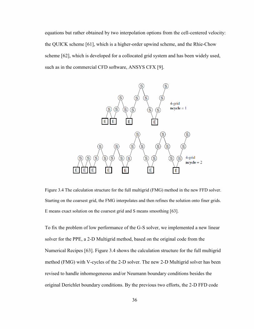
Figure 3.4 The calculation structure for the full multigrid (FMG) method in the new FFD
solver. Starting on the coarsest grid, the FMG interpolates and then refines the
solution onto finer grids. E means exact solution on the coarsest grid and S
means smoothing [63]. ...................................................................................... 36
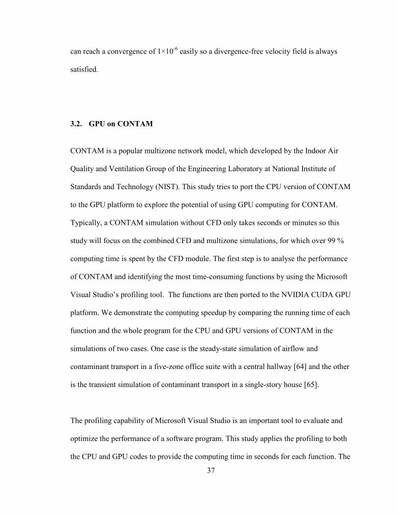
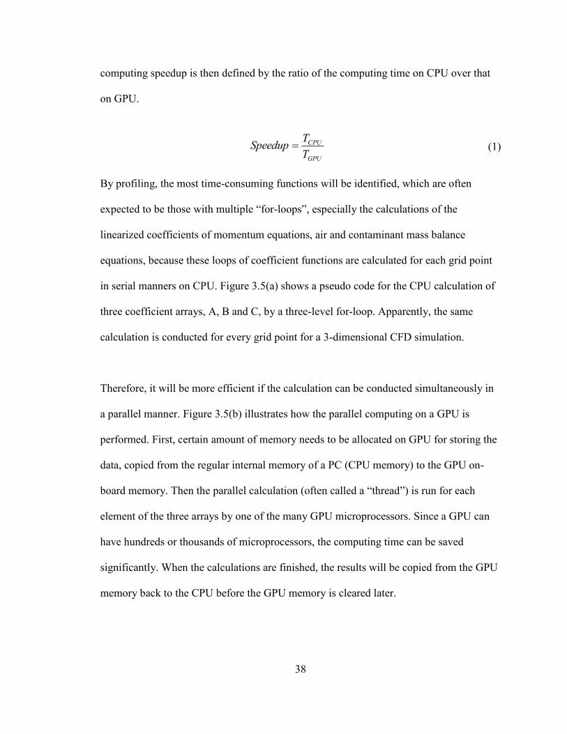
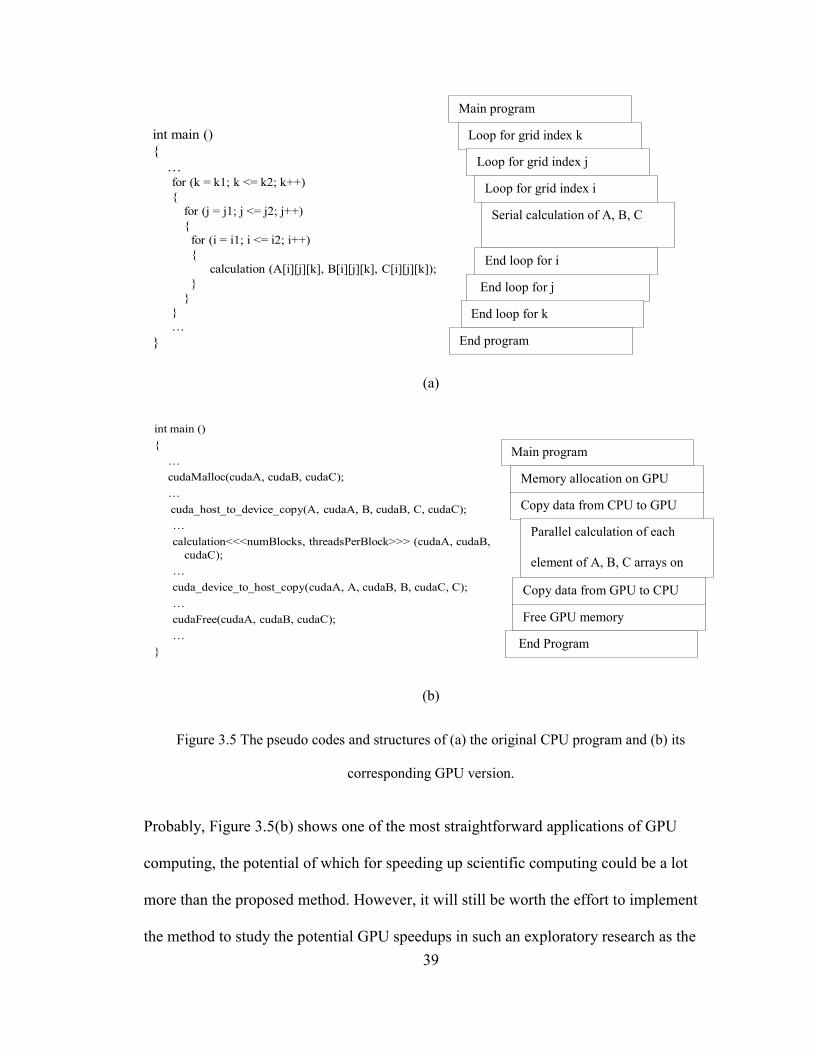
Figure 3.5 The pseudo codes and structures of (a) the original CPU program and (b) its
corresponding GPU version. ............................................................................. 39
Figure 3.6 Main procedures of transferring SketchUp model information to FFD data. . 40
Figure 3.7 FFD SketchUp plug-in grid creating screenshot and input dialogue window. 41
Figure 3.8 Process of converting SketchUp model information into FFD readable data . 42
Figure 4.1 Five-zone office suite case of CONTAM ........................................................ 44
Figure 4.2 Single-story house case of CONTAM ............................................................. 44
vii
Figure 4.3 Percentile computing time for each function of the CFD module of CONTAM
after the profiling in the case of the five-zone office suite with a grid resolution
of 42 × 24 × 24 (x × y × z) ................................................................................ 46
Figure 4.4 The comparison of the absolute computing time in seconds for each function
between (a) the CPU version and (b) the GPU version of CONTAM in the case
of the five-zone office suite with a grid resolution of 84 × 48 × 48. ................ 47
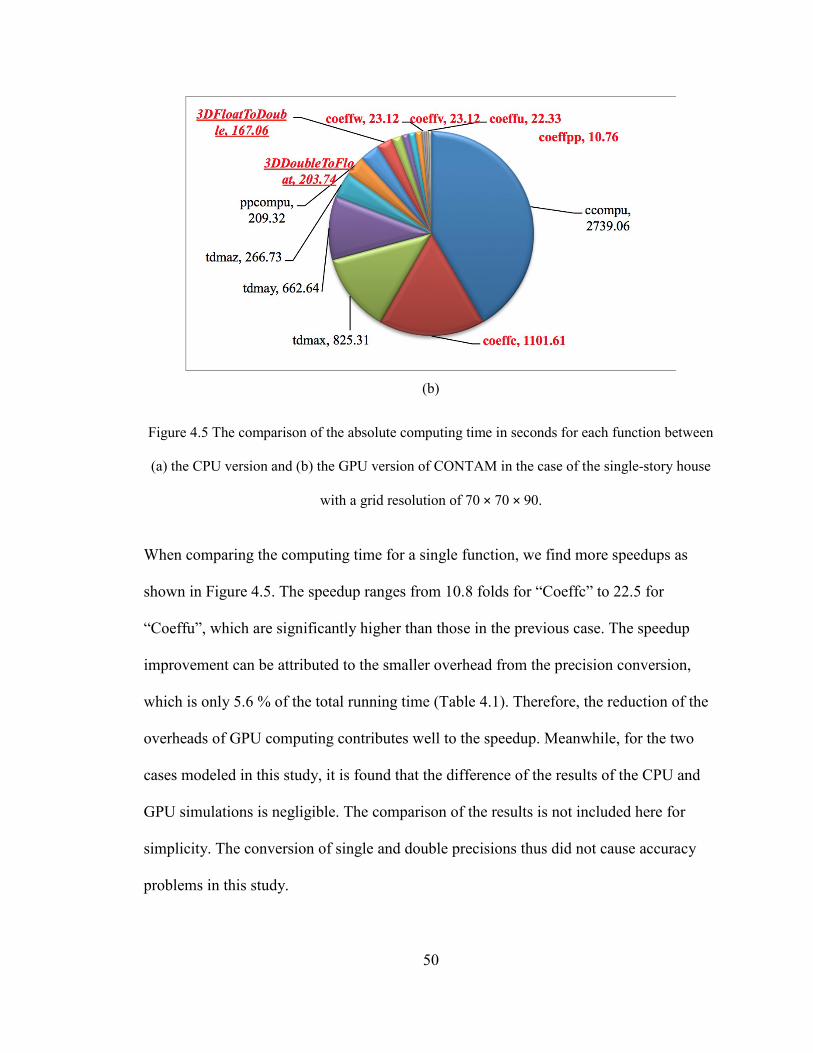
Figure 4.5 The comparison of the absolute computing time in seconds for each function
between (a) the CPU version and (b) the GPU version of CONTAM in the case
of the single-story house with a grid resolution of 70 × 70 × 90. ..................... 50
Figure 4.6 Vortex street in the wake of Selkirk Island [67] .............................................. 52
Figure 4.8 Screenshots of FFD simulation on Flow over a cylinder case ........................ 55
Figure 4.9 CFD simulation results by Sato and Kobayashi [69]. ..................................... 56
Figure 5.1 Air curtain working modes illustration............................................................ 58
Figure 5.2 Sketch of 2D Air curtain case .......................................................................... 59
Figure 5.3 Screenshot of the SketchUp model of Air curtain case ................................... 60
Figure 5.4 Screenshots of FFD velocity field comparison at V = 10 m/s ......................... 62
Figure 5.5 Screenshots of FFD comparison in concentration view at V = 10 m/s ............ 63
Figure 5.6 Screenshots of FFD velocity field comparison at θ = 15° ............................... 65
Figure 5.7 Screenshots of FFD comparison in concentration view atθ= 15° ................... 66
Figure 5.8 Screenshot for FFD simulation on Case f (V = 10 m/s, W = 0.2 m). ............... 67
Figure 5.9 Screenshots of FFD simulation on Case g (H = 2.5 m) ................................... 68
Figure 5.10 Screenshots of FFD simulation on Case h (U = 0.5 m/s) .............................. 68
Figure 5.11 Schematic diagram of wind pressure on building ......................................... 70
Figure 5.12 Basic patterns of building arrangement. ........................................................ 71
Figure 5.13 Sketch of building orientation to the wind direction ..................................... 72
Figure 5.16 Screenshots of FFD simulation on staggered building arrangement ............. 75
viii
Figure 5.17 Vertical view of aligned pattern simulation .................................................. 77
Figure 5.18 Simulation on Wind flow pass roofs ............................................................. 78
Figure 5.19 Sketch of opening positions........................................................................... 80
Figure 5.20 Screenshots of FFD simulation on different vent positions. ......................... 82
Figure 5.21 Screenshots of FFD simulation for case a with partition walls ..................... 83
Figure 5.22 Screenshots of FFD simulation for case a with different inlet angles ........... 84
Figure 5.23 Screenshots of user interaction on FFD simulation ....................................... 85
Appendices
Figure A.1 Screenshots of simulation on four enclosed building pattern at wind speed
6m/s, orientation 45º ....................................................................................... 103
Figure A.2 Mesh (left) and its configuration dialogue box (right) ................................. 105
Figure A.3 Steps for creating a box ................................................................................ 105
Figure A.4 Steps for creating a pitched roof ................................................................... 106
Figure A.5 Steps for creating vents................................................................................. 106
Figure A.6 Creating section plane for simulation ........................................................... 107
Figure A.7 FFD real-time simulation screenshot ............................................................ 108
ix
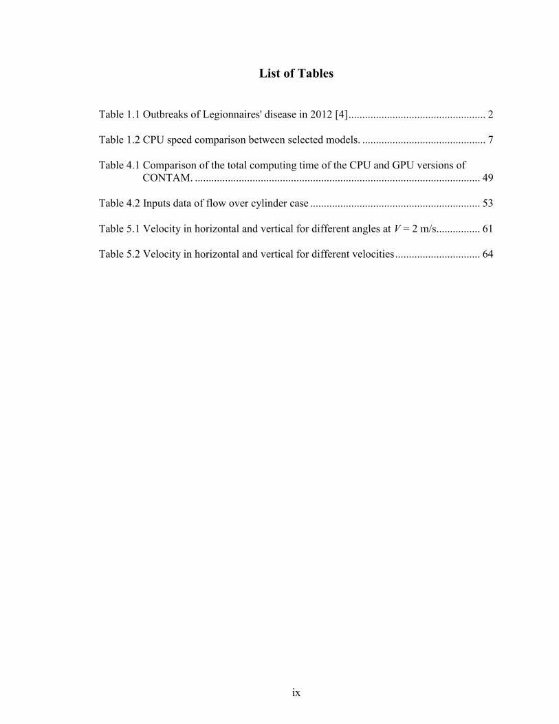
List of Tables
Table 1.1 Outbreaks of Legionnaires' disease in 2012 [4] .................................................. 2
Table 1.2 CPU speed comparison between selected models. ............................................. 7
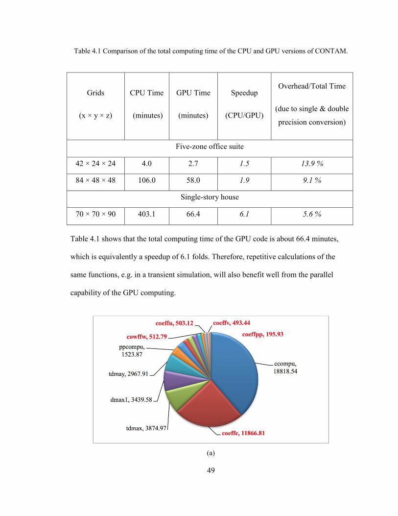
Table 4.1 Comparison of the total computing time of the CPU and GPU versions of
CONTAM. ........................................................................................................ 49
Table 4.2 Inputs data of flow over cylinder case .............................................................. 53
Table 5.1 Velocity in horizontal and vertical for different angles at V = 2 m/s................ 61
Table 5.2 Velocity in horizontal and vertical for different velocities ............................... 64
1
CHAPTER 1. INTRODUCTION
1.1. Problem Statement
Computer simulation of airflow in buildings has been widely used in modern building
designs and other related fields. With this technology, many problems associated with
building environment, such as building ventilation, fire and smoke control, have been
solved. However, with the increase of the complexity of the problems and elevated needs
for design analyses, the simulation speed of computer modeling often could not meet the
requirements in the current situation
1.2. Current Situation and Requirements
The issues in the field of building environment are gaining more and more attention in
modern building designs. For example, poor air quality and inadequate ventilation could
lead to many common health problems, such as irritations of the skin, eyes, nose and
throat; headaches; allergies; odor and more; all of these are all defined as Sick Building
Syndromes (SBS) by the World Health Organization in 1983 [1]. Those are not a single
syndrome but a combination of many ailments that cannot be simply diagnosed. Various
contaminants deposition and the ventilation system inefficiency are the main reasons. If
the indoor environment is suitable for the bacteria’s growth, further serious problems
may be detonated, such as the Legionnaires' disease and Pontiac fever that are classified
into Building Related Illness (BRI) [2]. Legionnaires' disease is a fatal illness. It is
2
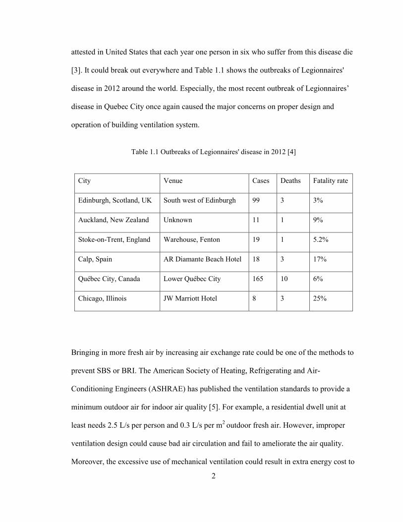
attested in United States that each year one person in six who suffer from this disease die
[3]. It could break out everywhere and Table 1.1 shows the outbreaks of Legionnaires'
disease in 2012 around the world. Especially, the most recent outbreak of Legionnaires’
disease in Quebec City once again caused the major concerns on proper design and
operation of building ventilation system.
Table 1.1 Outbreaks of Legionnaires' disease in 2012 [4]
City Venue Cases Deaths Fatality rate
Edinburgh, Scotland, UK South west of Edinburgh 99 3 3%
Auckland, New Zealand Unknown 11 1 9%
Stoke-on-Trent, England Warehouse, Fenton 19 1 5.2%
Calp, Spain AR Diamante Beach Hotel 18 3 17%
Québec City, Canada Lower Québec City 165 10 6%
Chicago, Illinois JW Marriott Hotel 8 3 25%
Bringing in more fresh air by increasing air exchange rate could be one of the methods to
prevent SBS or BRI. The American Society of Heating, Refrigerating and Air-
Conditioning Engineers (ASHRAE) has published the ventilation standards to provide a
minimum outdoor air for indoor air quality [5]. For example, a residential dwell unit at
least needs 2.5 L/s per person and 0.3 L/s per m2
outdoor fresh air. However, improper
ventilation design could cause bad air circulation and fail to ameliorate the air quality.
Moreover, the excessive use of mechanical ventilation could result in extra energy cost to
3
a building.
From Arthur M. Kodama and Robert I. McGee’s research [6], the air-conditioned houses
are reported having more health complaints than naturally ventilated houses. The
occupants in air-conditioned rooms get more chance to have eye irritation, sneezing,
nasal congestion, morning cough, and morning phlegm. They also found that the total
number of bacterial particulates in air-conditioned room is much higher than that in
outdoors and naturally ventilated rooms.
Inefficient ventilation could also increase energy consumption. Research shows that
indoor and outdoor air-exchange accounts for as much as 50% of building total energy
consumptions [7]. The heater warms up the new intake air in the winter or the air-
conditioner cools down the new intake air in the summer, which causes the energy
consumption. The more air is exchanged, the more energy is consumed. To meet the
ventilation standards, an inefficient ventilation design has to bring more outdoor-air into
the inside, which could cause more energy load in the building.
To have buildings with better indoor environment and less energy consumption, good
designs combined with high efficiently natural ventilation and mechanical ventilation are
critical. However, there is no simple universal solution that could fit all the designs,
because each space has its own characteristics. Room dimensions and location, vent
positions and sizes, wind directions and speeds, all the factors above constitute the
uniqueness of a building. The best way for each specific building design is to analyze its
own airflow and provide specific ventilation solution. Therefore, a computer simulation,
which can provide fast analysis with acceptable accuracy, is preferred so that different
4
design scenarios can be studied and compared to provide a best solution during an
architectural design.
1.3. Computational Fluid Dynamics
1.3.1 CFD Introduction
For decades, one of the most popular methods in building airflow analysis is
computational fluid dynamics (CFD), which solves the Navier-Stoke equations and other
associated equations on many mesh grids, is used in computer simulation for fluid flows
to achieve better results. The most widely used CFD programs such as ANSYS Fluent [8]
and CFX [9], CHAM PHOENICS [10], and Wind Perfect [11], etc. are all based on CFD
solver. Some program has a CFD component, such as CONTAM [12].
ANSYS Fluent is a general purpose fluid flow simulation software. It could simulate
complex models and provide accurate CFD results [8]. CFX is also a general purpose
CFD software of ANSYS. It provide more accurate results [9]. CHAM PHOENICS is a
CFD tool that simulates mainly about “fluid flow, heat or mass transfer, chemical
reaction and combustion” in building environment and engineering equipment [10]. Wind
Perfect is also a CFD-based software that specially focuses on the building environment
airflow simulation [11]. It is well known in Japan and China. CONTAM is a “multizone
indoor air quality and ventilation analysis computer program” [12]. It could simulate
airflows in the building, determine contaminant concentrations, predict personal exposure
to airborne contaminant, and model fire smoke transport for fire safety designs. After the
5
version 3.0, CFD has become a main function in the software.
1.3.2 CFD Limitations
CFD could generate accurate results and detailed information about fluid motion,
temperature distributions and other characteristics. Higher accuracy of CFD calculations
requires higher-order integration method, finer grid size and other parameters, but it
depends on more computing time if the grid amount is huge. For example, a three-hour
simulation of an indoor auto-racing complex with a 100×100×55 grid resolution in
steady-state conditions, a CFD program requires about 10 hours to generate a satisfied
result [13].
Therefore, CFD is often not favored, especially in the early stage of building design when
designers concern more about computing speed because of frequent modification. Once
the pattern and structure of an architectural design are finalized, there could be limited
space left for optimizing the ventilation design.
In order to change the situation, many people are dedicated to improve the CFD
simulation speed. One of the current trends of the endeavors is to achieve real-time or
fast-than-real-time simulation. There are many advantages on real-time simulation. It is
not only about to save our waiting time; it could also change the way of designing and
analyzing of building airflows. For example, a fast-than-real-time simulation can be used
to predict the smoke and contaminant transport at real time in an existent building. If the
prediction is accurate and informative, emergency management personnel can use the
prediction to take proper measures to prevent the occurrence of disasters; with the
6
accurate predicted information, the emergency control personnel can direct occupants to
evacuate correctly in the buildings during accidents, and therefore minimize the
casualties and cost.
Compared to CFD, other computer models such as multizone models [14] and zonal
models [15], could provide fast results, because they have some simple uniform
assumptions. However, the results they provided are not as informative [16] and accurate
as CFD because the grid resolution needs to be coarse enough (e.g. one node in a
multizone mdel) to achieve the fast speed [17]. Hence these models are not competent,
and an intermediate method is required with both fast speed and acceptable accuracy.
With current technologies, there are often two popular ways which could be combined
together to speed up the CFD simulation or even realize the real-time simulation, and also
with an acceptable accuracy. One method is to redirect the program, which often runs on
the Central Processing Unit (CPU) of a computer to run on Graphic Processing Unit
(GPU) to speed up the simulation; the other one is to use some advanced CFD algorithms,
such as the Fast Fluid Dynamics (FFD) algorithm, to accelerate the calculation.
1.4. Central Processing Unit (CPU) Computing
The CPU, which is in charge of the basic arithmetical, logical computation and
input/output operation, is considered as the core hardware in a computer system. From
1960s to now, the CPU has changed from several printed circuit boards to a smaller than
four square centimeters microprocessor and achieved great speed enhancement.
The current CFD calculations are mostly run on the CPUs. The performance of the CPU
7
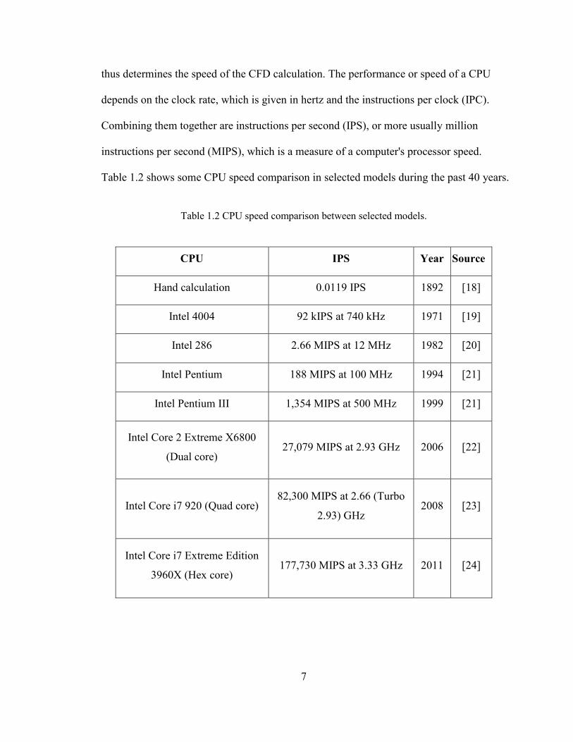
thus determines the speed of the CFD calculation. The performance or speed of a CPU
depends on the clock rate, which is given in hertz and the instructions per clock (IPC).
Combining them together are instructions per second (IPS), or more usually million
instructions per second (MIPS), which is a measure of a computer's processor speed.
Table 1.2 shows some CPU speed comparison in selected models during the past 40 years.
Table 1.2 CPU speed comparison between selected models.
CPU IPS Year Source
Hand calculation 0.0119 IPS 1892 [18]
Intel 4004 92 kIPS at 740 kHz 1971 [19]
Intel 286 2.66 MIPS at 12 MHz 1982 [20]
Intel Pentium 188 MIPS at 100 MHz 1994 [21]
Intel Pentium III 1,354 MIPS at 500 MHz 1999 [21]
Intel Core 2 Extreme X6800
(Dual core) 27,079 MIPS at 2.93 GHz 2006 [22]
Intel Core i7 920 (Quad core) 82,300 MIPS at 2.66 (Turbo
2.93) GHz 2008 [23]
Intel Core i7 Extreme Edition
3960X (Hex core) 177,730 MIPS at 3.33 GHz 2011 [24]
8
Although there has been a great enhancement on CPU’s performance, the CFD
calculation speed still could not reach to real-time simulation on a PC, especially when
the model is complex and large. Although CFD simulations can be run on large scale
computer clusters to accelerate the speed, these resources are expensive and often not
accessible to common building designers. Therefore, most of building airflow analysis in
a design firm has to be done on a PC. CPU has limited ability to operate many tasks in
the same time and limited improvement space with current technology. Therefore, the
graphic processing unit could be introduced to accelerate the calculation.
1.5. Graphic Processing Unit (GPU) Computing
As mentioned previously, rapid simulations are traditionally performed by using parallel
computer clusters, which limit the use of parallel applications to those who have access to
such clusters. An alternative approach is becoming possible due to the advent of multi-
core GPUs, which are readily available on desktop computers.
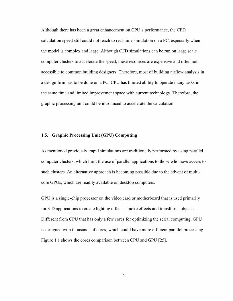
GPU is a single-chip processor on the video card or motherboard that is used primarily
for 3-D applications to create lighting effects, smoke effects and transforms objects.
Different from CPU that has only a few cores for optimizing the serial computing, GPU
is designed with thousands of cores, which could have more efficient parallel processing.
Figure 1.1 shows the cores comparison between CPU and GPU [25].
9
Figure 1.1 Cores comparison between CPU and GPU[25]
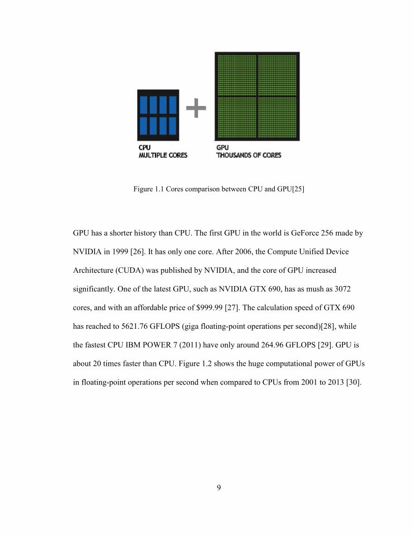
GPU has a shorter history than CPU. The first GPU in the world is GeForce 256 made by
NVIDIA in 1999 [26]. It has only one core. After 2006, the Compute Unified Device
Architecture (CUDA) was published by NVIDIA, and the core of GPU increased
significantly. One of the latest GPU, such as NVIDIA GTX 690, has as mush as 3072
cores, and with an affordable price of $999.99 [27]. The calculation speed of GTX 690
has reached to 5621.76 GFLOPS (giga floating-point operations per second)[28], while
the fastest CPU IBM POWER 7 (2011) have only around 264.96 GFLOPS [29]. GPU is
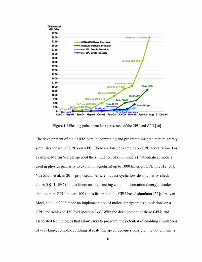
about 20 times faster than CPU. Figure 1.2 shows the huge computational power of GPUs
in floating-point operations per second when compared to CPUs from 2001 to 2013 [30].
10
Figure 1.2 Floating-point operations per second of the CPU and GPU [30]
The development of the CUDA parallel computing and programming architecture greatly
simplifies the use of GPUs on a PC. There are lots of examples on GPU acceleration. For
example, Martin Weigel speeded the simulation of spin models (mathematical models
used in physics primarily to explain magnetism) up to 1000 times on GPU in 2012 [31];
Yue Zhao, et al. in 2011 proposed an efficient quasi-cyclic low-density parity-check
codes (QC-LDPC Code, a linear error correcting code in information theory) decoder
simulator on GPU that are 100 times faster than the CPU-based simulator [32]; J.A. van
Meel, et al. in 2008 made an implementation of molecular dynamics simulations on a
GPU and achieved 150 fold speedup [33]. With the development of these GPUs and
associated technologies that allow users to program, the potential of enabling simulations
of very large, complex buildings at real-time speed becomes possible; the bottom line is
11
that it could decrease the simulation time of current building simulations in many cases.
1.6. Fast Fluid Dynamics (FFD)
Stam developed a stable fluid solver for modeling fluid flow and heat transfer for the
applications in computer games in 1999 [34]. With this method, players in the computer
game could get real-time response when they make interactions with the computer. The
method is real-time or more than real time fast even on a PC with a single CPU. Many
people have used Stam’s method to realize real-time simulations and some of them have
improved it. For example in 2003, Mark J. Harris et al. simulated three-dimensional
visually realistic interactive clouds and applied it on GPU [35]. In the same year, Nick
Rasmussen et al. improved the algorithm for simulating highly detailed large scale
phenomemon such as the nuclear explosions [36]. In 2005, Nelson S.H. Chu and Chiew-
Lan Tai simulated ink dispersion in absorbent paper for art such as eastern ink painting
[37].
Based on the same techniques of Stam’s, an improved method called FFD was proposed
by Zuo and Chen in 2007 for indoor airflow simulations [38]. This new algorithm, which
is based on the Navier-Stokes equations, could simulate the building airflows in real-time.
Their method is based on a simple linear solver and only demonstrated in a few simple
typical flow problems. The application of the FFD to real building airflow analysis needs
a faster solver and more general and complex cases for real design practices. In this thesis
study, a faster method for simulating the air and contaminant movement related to
buildings is developed. This new method can realize a real-time simulation. The method
12
will be applied to a few general design studies in the field of building simulations so that
it will help to bring the engineering design concepts in the early stage of building designs.
1.7. Objectives
The objectives of this thesis are:
To illustrate the theories and methodology of speeding up the building airflow
simulations. It also includes the literature review, our improvements and relevant
computer language codes and equations.
To compare the speed in different simulation cases. The comparisons are between
CONTAM running on CPU and GPU, FFD and CFD (or experimental data). The
correlated figures and tables of the cases are attached to help on analyzing the
simulation results.
To apply the FFD program to the applications in different building related fields.
Several cases in different fields are simulated by FFD to show its function and
capability, especially for architects applying the FFD method into their concept
design to improve the building environment. For practical use of the FFD algorithm,
a SketchUp FFD plug-in is developed for designers and engineers.
1.8. Thesis Outline
This thesis is divided into six chapters to illustrate the author’s effort on improving the
speed and accuracy of airflow simulation in buildings. The current chapter presents the
13
current problems and requirements of accelerating the airflow simulation. It introduces
the background knowledge of fluid simulation, and illustrates the objectives of the thesis.
Chapter 2 represents a literature review of current research using GPU and FFD to
accelerate the fluid dynamic simulations. The detail information of GPU and FFD is
illustrated. Several cases are also introduced in this part. At the end of this chapter, the
efforts, which have been done in this study to improve the simulation, are summarized in
steps. Three improvements are mainly presented: rewriting CONTAM on GPU,
interaction interface on FFD, and some applications.
Chapter 3 introduces the theory and methodology on rewriting CPU-based program to
GPU, using GPU and FFD to accelerate the simulation, and user and PC real-time
interactions. Detailed computer language codes and fluid dynamic equations are
demonstrated. All the numerical experiments and the comparisons accomplished
afterward are based on the validity of the theories and methodology. A FFD SketchUp
plug-in, which is specially designed for creating models, is introduced also in this part.
Chapter 4 is the results and discussion part. In this chapter, several cases are compared to
show whether GPU or CPU for CONTAM is faster, and how FFD achieves real-time
simulations. The accuracy of the simulations has also been shown by the comparisons.
Chapter 5 illustrates some applications of the FFD program. The speed, accuracy and
convenience of operation are featured. It also discusses many other possibilities in
various fields.
Chapter 6 concludes the thesis with suggested future studies.
14
CHAPTER 2. LITERATURE REVIEW
In Chapter 1, some basic information of accelerating the airflow simulation has been
introduced. In this chapter, the detailed information related to building environment and
ventilation will be reviewed for two methods: GPU computing and FFD. The GPU
computing represents the improvements from the computer hardware and FFD is related
to the new algorithms developed so far in the literature.
2.1. GPU Acceleration
2.1.1 Overview of CFD on GPU
Since GPU could significantly increase the performance of computing, many projects are
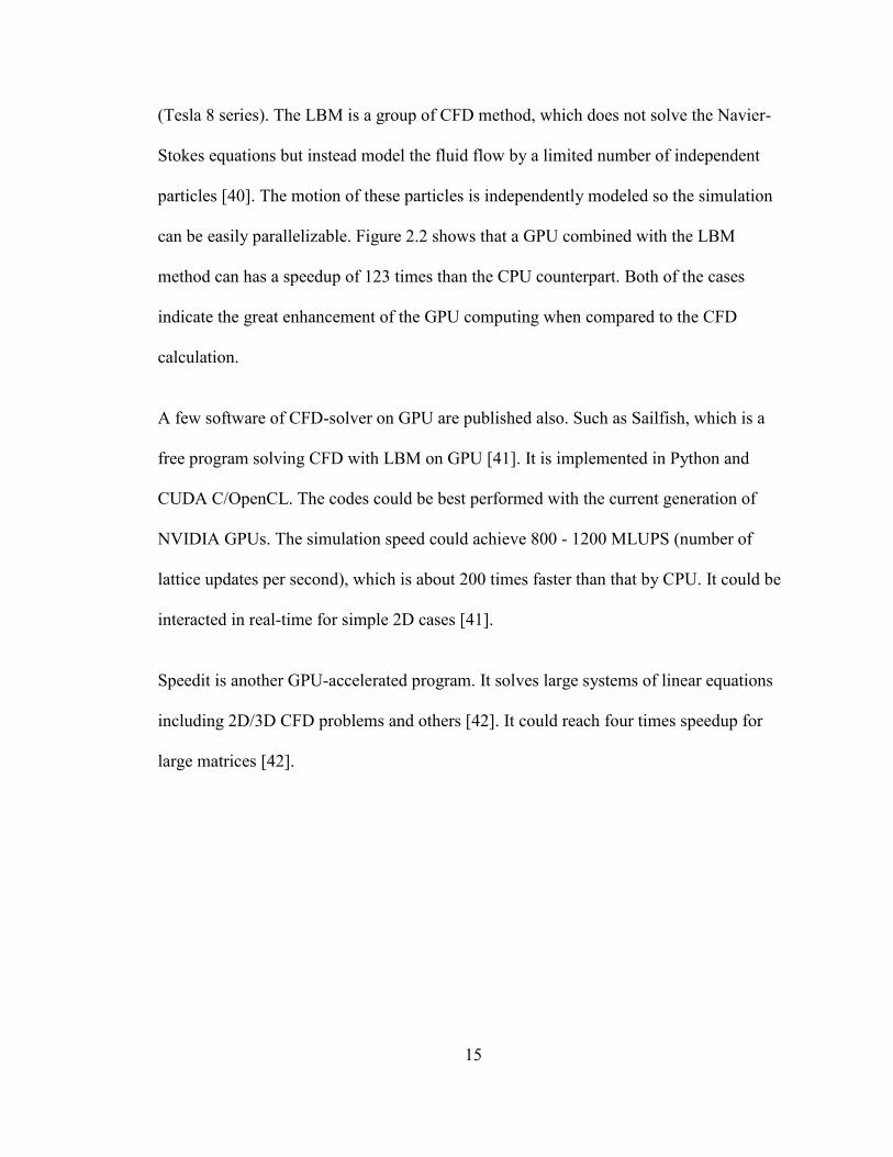
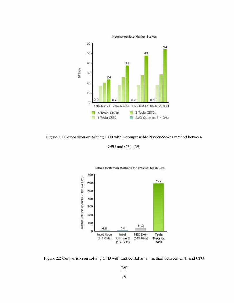
aiming to accelerate CFD with CUDA-enabled GPUs. Figure 2.1 and 2.2 show the GPU
implement of two CFD methods [39]. Figure 2.1 is the incompressible Navier-Stokes
method, comparing between different numbers of GPUs (Tesla C870) and one CPU
(AMD Opteron 2.4GHz). It shows that the GPU speedup can be as high as 108 times than
the CPU simulation. The speedup also increases with the grid resolutions: more grid
numbers better take advantages of the GPU parallel computing capabilities. This is
surprisingly different from the normal CPU simulations, of which the computing speed is
often reduced by the increased number of grids. If GPU is combined with an advanced
algorithm to make full use of the parallel capability, the speedup can be even better.
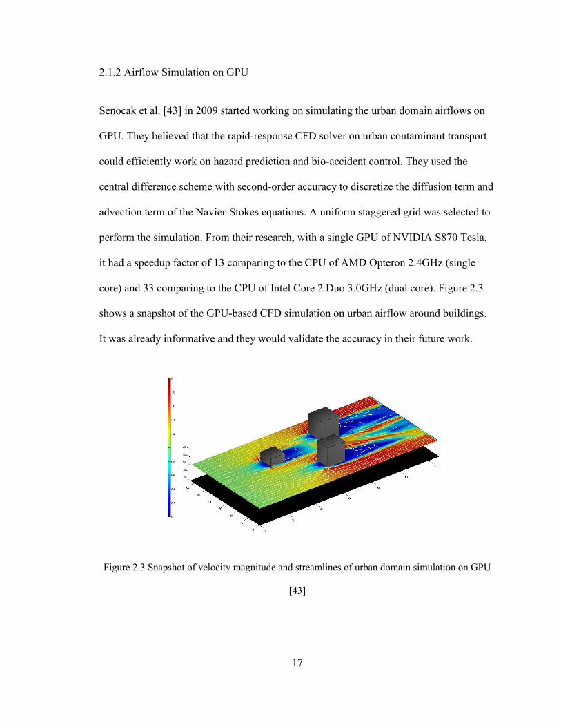
Figure 2.2 is the Lattice Boltzman methods (LBM), comparing between 3 different CPUs
(Intel Xeon 3.4 GHz, Intel Itanium 2 1.4 GHz and NEC SX6+ 565 MHz) and one GPU
15
(Tesla 8 series). The LBM is a group of CFD method, which does not solve the Navier-
Stokes equations but instead model the fluid flow by a limited number of independent
particles [40]. The motion of these particles is independently modeled so the simulation
can be easily parallelizable. Figure 2.2 shows that a GPU combined with the LBM
method can has a speedup of 123 times than the CPU counterpart. Both of the cases
indicate the great enhancement of the GPU computing when compared to the CFD
calculation.
A few software of CFD-solver on GPU are published also. Such as Sailfish, which is a
free program solving CFD with LBM on GPU [41]. It is implemented in Python and
CUDA C/OpenCL. The codes could be best performed with the current generation of
NVIDIA GPUs. The simulation speed could achieve 800 - 1200 MLUPS (number of
lattice updates per second), which is about 200 times faster than that by CPU. It could be
interacted in real-time for simple 2D cases [41].
Speedit is another GPU-accelerated program. It solves large systems of linear equations
including 2D/3D CFD problems and others [42]. It could reach four times speedup for
large matrices [42].
16
Figure 2.1 Comparison on solving CFD with incompressible Navier-Stokes method between
GPU and CPU [39]
Figure 2.2 Comparison on solving CFD with Lattice Boltzman method between GPU and CPU
[39]
17
2.1.2 Airflow Simulation on GPU
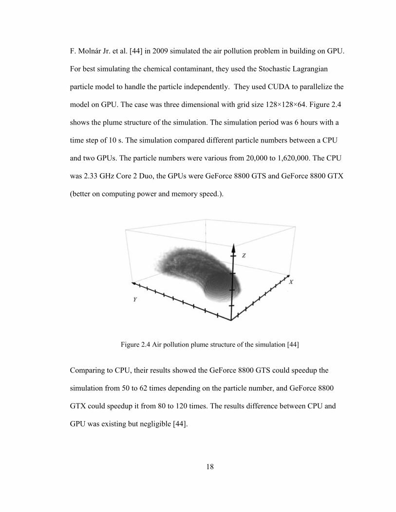
Senocak et al. [43] in 2009 started working on simulating the urban domain airflows on
GPU. They believed that the rapid-response CFD solver on urban contaminant transport
could efficiently work on hazard prediction and bio-accident control. They used the
central difference scheme with second-order accuracy to discretize the diffusion term and
advection term of the Navier-Stokes equations. A uniform staggered grid was selected to
perform the simulation. From their research, with a single GPU of NVIDIA S870 Tesla,
it had a speedup factor of 13 comparing to the CPU of AMD Opteron 2.4GHz (single
core) and 33 comparing to the CPU of Intel Core 2 Duo 3.0GHz (dual core). Figure 2.3
shows a snapshot of the GPU-based CFD simulation on urban airflow around buildings.
It was already informative and they would validate the accuracy in their future work.
Figure 2.3 Snapshot of velocity magnitude and streamlines of urban domain simulation on GPU
[43]
18
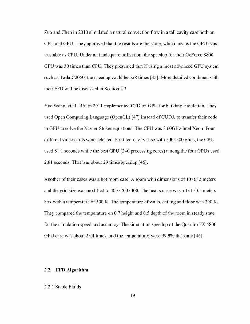
F. Moln r r. et al. [44] in 2009 simulated the air pollution problem in building on GPU.
For best simulating the chemical contaminant, they used the Stochastic Lagrangian
particle model to handle the particle independently. They used CUDA to parallelize the
model on GPU. The case was three dimensional with grid size 128×128×64. Figure 2.4
shows the plume structure of the simulation. The simulation period was 6 hours with a
time step of 10 s. The simulation compared different particle numbers between a CPU
and two GPUs. The particle numbers were various from 20,000 to 1,620,000. The CPU
was 2.33 GHz Core 2 Duo, the GPUs were GeForce 8800 GTS and GeForce 8800 GTX
(better on computing power and memory speed.).
Figure 2.4 Air pollution plume structure of the simulation [44]
Comparing to CPU, their results showed the GeForce 8800 GTS could speedup the
simulation from 50 to 62 times depending on the particle number, and GeForce 8800
GTX could speedup it from 80 to 120 times. The results difference between CPU and
GPU was existing but negligible [44].
19
Zuo and Chen in 2010 simulated a natural convection flow in a tall cavity case both on
CPU and GPU. They approved that the results are the same, which means the GPU is as
trustable as CPU. Under an inadequate utilization, the speedup for their GeForce 8800
GPU was 30 times than CPU. They presumed that if using a most advanced GPU system
such as Tesla C2050, the speedup could be 558 times [45]. More detailed combined with
their FFD will be discussed in Section 2.3.
Yue Wang, et al. [46] in 2011 implemented CFD on GPU for building simulation. They
used Open Computing Language (OpenCL) [47] instead of CUDA to transfer their code
to GPU to solve the Navier-Stokes equations. The CPU was 3.60GHz Intel Xeon. Four
different video cards were selected. For their cavity case with 500×500 grids, the CPU
used 81.1 seconds while the best GPU (240 processing cores) among the four GPUs used
2.81 seconds. That was about 29 times speedup [46].
Another of their cases was a hot room case. A room with dimensions of 10×6×2 meters
and the grid size was modified to 400×200×400. The heat source was a 1×1×0.5 meters
box with a temperature of 500 K. The temperature of walls, ceiling and floor was 300 K.
They compared the temperature on 0.7 height and 0.5 depth of the room in steady state
for the simulation speed and accuracy. The simulation speedup of the Quardro FX 5800
GPU card was about 25.4 times, and the temperatures were 99.9% the same [46].
2.2. FFD Algorithm
2.2.1 Stable Fluids
20
Stable fluids algorithm, which is based on a so-called Semi-Lagrangian technique to
consider the convection term in the Navier-Stokes equations to achieve real-time
simulation, was first time proposed for games by Jos Stam in 1999. The new method
could solve the full Navier-Stokes equations in real-time with three-dimensional fluids,
because it can use a large time-step stably, a projection method for the pressure-velocity
coupling, and both Semi-Lagrangian for the convection term and the implicit methods for
the diffusion term [48]. Because all these algorithms give only the approximation
solutions, it was hence not as accurate as the normal CFD methods. However, for the low
accurate applications such as computer games, the accuracy is not the major concern but
the visual effect instead. Stam’s algorithm has provided a perfect solution to this problem.
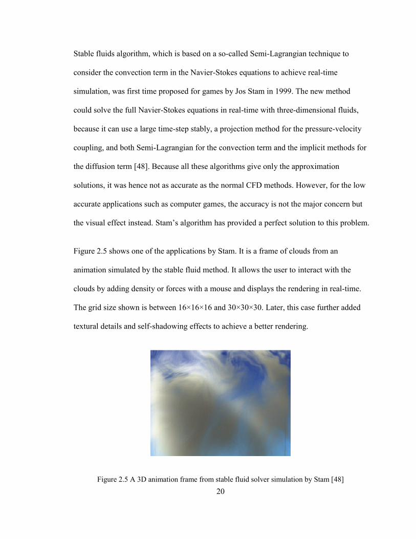
Figure 2.5 shows one of the applications by Stam. It is a frame of clouds from an
animation simulated by the stable fluid method. It allows the user to interact with the
clouds by adding density or forces with a mouse and displays the rendering in real-time.
The grid size shown is between 16×16×16 and 30×30×30. Later, this case further added
textural details and self-shadowing effects to achieve a better rendering.
Figure 2.5 A 3D animation frame from stable fluid solver simulation by Stam [48]
21
Based on his method of stable fluids, Stam in 2001 provided a much simpler fluid solver
for fluids wrapped around in space. With the FFTW (Fast Fourier Transform west, a free
black box software to switch between the spatial and the Fourier domain), one page of C
code is enough for the solver [49]. Although this method is not accurate enough, the fast
speed encourages many users and developers to improve it in their own fields.
2.2.2 FFD in Indoor Air
In 2007, Zuo and Chen developed the Fast Fluid Dynamics (FFD) based on the Semi-
Lagrangian approach [50]. They validated the FFD accuracy with experimental data and
other CFD simulations for several 2-D indoor airflow simulation cases. The results
showed an acceptable accuracy and all of them achieved the speed faster than real time.
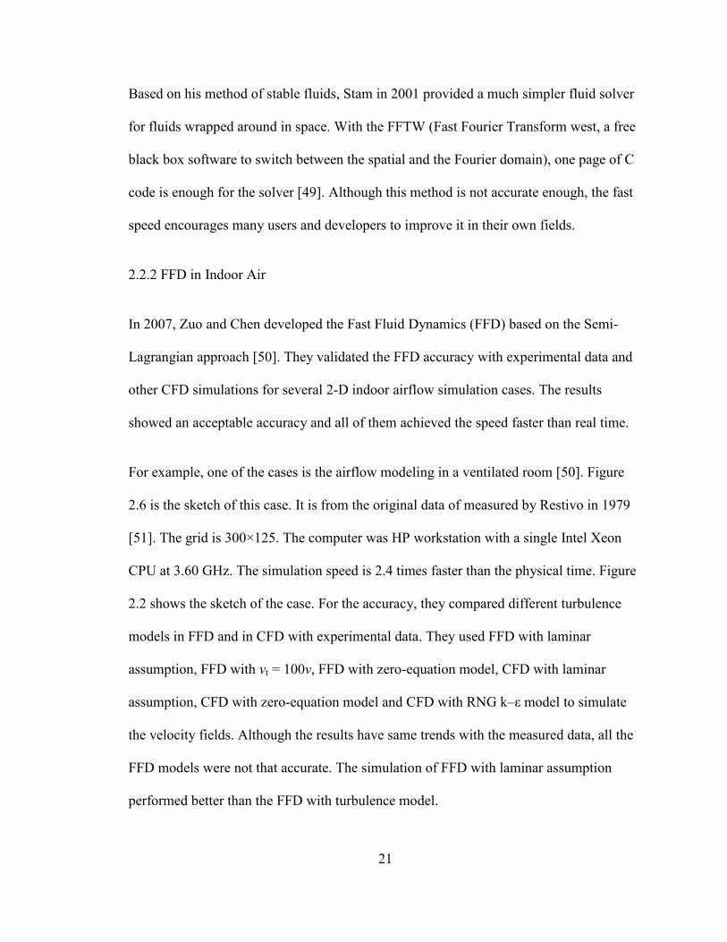
For example, one of the cases is the airflow modeling in a ventilated room [50]. Figure
2.6 is the sketch of this case. It is from the original data of measured by Restivo in 1979
[51]. The grid is 300×125. The computer was HP workstation with a single Intel Xeon
CPU at 3.60 GHz. The simulation speed is 2.4 times faster than the physical time. Figure
2.2 shows the sketch of the case. For the accuracy, they compared different turbulence
models in FFD and in CFD with experimental data. They used FFD with laminar
assumption, FFD with vt = 100v, FFD with zero-equation model, CFD with laminar
assumption, CFD with zero-equation model and CFD with RNG k–ε model to simulate
the velocity fields. Although the results have same trends with the measured data, all the
FFD models were not that accurate. The simulation of FFD with laminar assumption
performed better than the FFD with turbulence model.
22
Figure 2.6 The sketch of empty room with ventilation [51]
In their later study, more cases were compared in detailed ways. They found that the
simulation of FFD without turbulence model performed faster and better in accuracy than
the FFD with turbulence model. Although comparing to CFD, the FFD had less accuracy,
the speed of the FFD simulation was about 50 times faster than the CFD simulation [50].
To enhance the accuracy of FFD, W. Zuo et al. in 2010 made some improvements in their
later research. They adjusted the equation solving steps and removed one additional
projection step to decrease the simulation speed. They found that using finite volume of
discretization scheme rather than finite difference could generate better accuracy. The
improvement of mass conservation between the inlets and outlets can also improve the
accuracy [52]. The theories will be discussed in section 3.1.
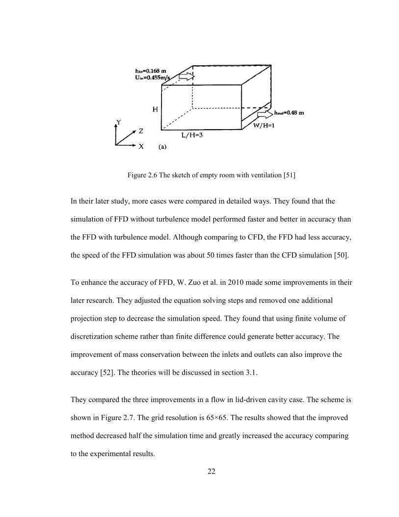
They compared the three improvements in a flow in lid-driven cavity case. The scheme is
shown in Figure 2.7. The grid resolution is 65×65. The results showed that the improved
method decreased half the simulation time and greatly increased the accuracy comparing
to the experimental results.
23
Figure 2.7 Scheme of the flow in a lid-driven cavity case [52]
With the all improvements together, they redid the airflow modeling in a ventilated room
case. The results were much closer to the experimental data [52].
2.3. FFD on GPU
To further increase the computing speed, Zuo and Chen in 2010 emphasized their effort
on developing the FFD algorithm on GPU [45][53]. Some indoor cases such as flow in a
lid driven cavity and natural convection in a tall cavity were compared between running
on CPU and GPU. The CPU was INTEL Core 2 Duo 3.0GHz (32 GFLOPS) and the GPU
was NVIDIA GeForce 8800 GTX (367 GFLOPS). For the flow in the lid driven cavity
case, they used a fine grid resolution of 513×513 for Re = 10000 and 65×65 for Re = 100.
The GPU version of FFD performed well in both turbulent and laminar flow comparing
with the high quality CFD results [53].
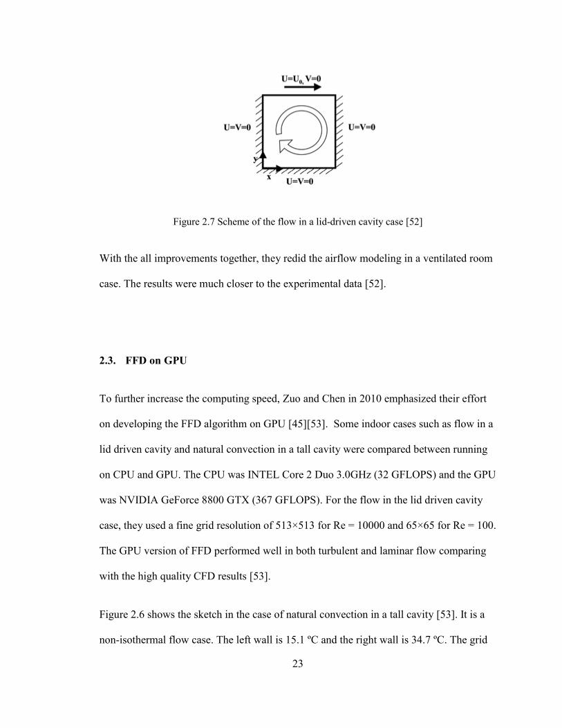
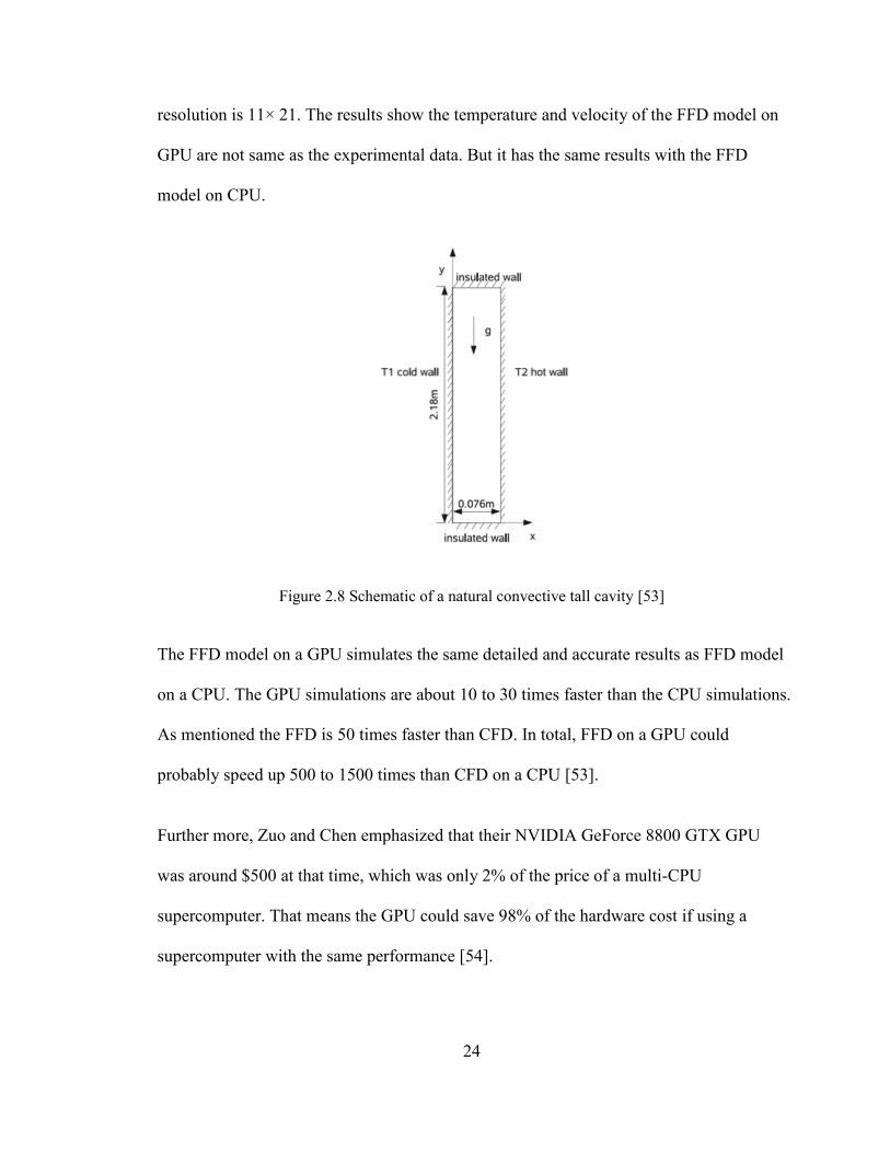
Figure 2.6 shows the sketch in the case of natural convection in a tall cavity [53]. It is a
non-isothermal flow case. The left wall is 15.1 ºC and the right wall is 34.7 ºC. The grid
24
resolution is 11× 21. The results show the temperature and velocity of the FFD model on
GPU are not same as the experimental data. But it has the same results with the FFD
model on CPU.
Figure 2.8 Schematic of a natural convective tall cavity [53]
The FFD model on a GPU simulates the same detailed and accurate results as FFD model
on a CPU. The GPU simulations are about 10 to 30 times faster than the CPU simulations.
As mentioned the FFD is 50 times faster than CFD. In total, FFD on a GPU could
probably speed up 500 to 1500 times than CFD on a CPU [53].
Further more, Zuo and Chen emphasized that their NVIDIA GeForce 8800 GTX GPU
was around $500 at that time, which was only 2% of the price of a multi-CPU
supercomputer. That means the GPU could save 98% of the hardware cost if using a
supercomputer with the same performance [54].
25
2.4. Our Improvements
The literature review shows that the applications of both GPU and FFD to building
airflow simulations are fairly limited. There is some ongoing research however these
studies are mostly preliminary, applied only to simple cases, and they are restricted to
certain self-developed codes.
This thesis is trying to investigate further applications of both GPU and FFD to building
airflow simulations. It focuses on four major improvements:
use GPU computing for a general public domain program, CONTAM;
further development of Stam’s finite difference FFD algorithms instead of finite
volume method;
development of a graphical interface for FFD by using SketchUp plug-in;
applications of both GPU and FFD to more general and practical design problems.
The details will be illustrated in the next three chapters.
2.5. Conclusion
This chapter reviews the progress in the literature on both the GPU computing
acceleration and FFD algorithms. Many investigators in different fields have involved
themselves into these technologies and made great progress in the past few years. The
GPU computing could speedup 10 to 100 times comparing to CPU computing. The FFD
could speedup at least 50 times than CFD. They provide one of the good solutions to
achieve real-time building airflow simulations.
26
CHAPTER 3. METHODOLOGY
3.1. Background Theory on FFD
3.1.1 Governing Equations on FFD
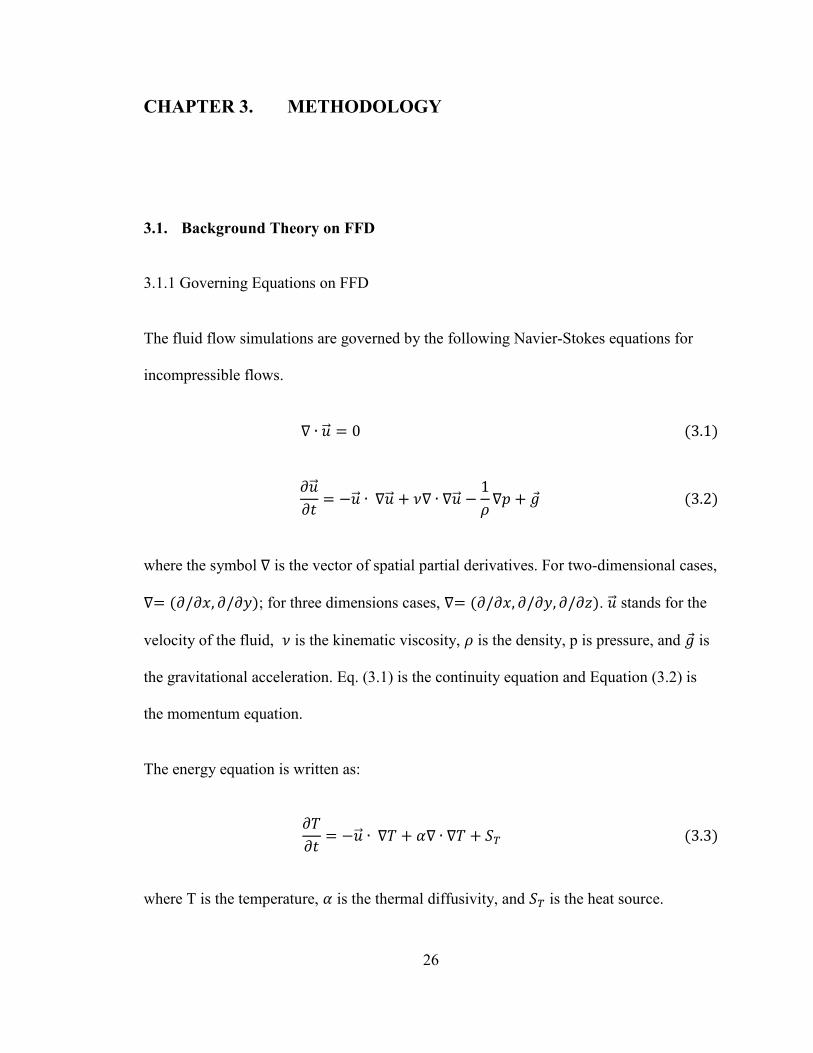
The fluid flow simulations are governed by the following Navier-Stokes equations for
incompressible flows.
where the symbol is the vector of spatial partial derivatives. For two-dimensional cases,
; for three dimensions cases, . stands for the
velocity of the fluid, is the kinematic viscosity, is the density, p is pressure, and is
the gravitational acceleration. Eq. (3.1) is the continuity equation and Equation (3.2) is
the momentum equation.
The energy equation is written as:
where T is the temperature, is the thermal diffusivity, and is the heat source.
27
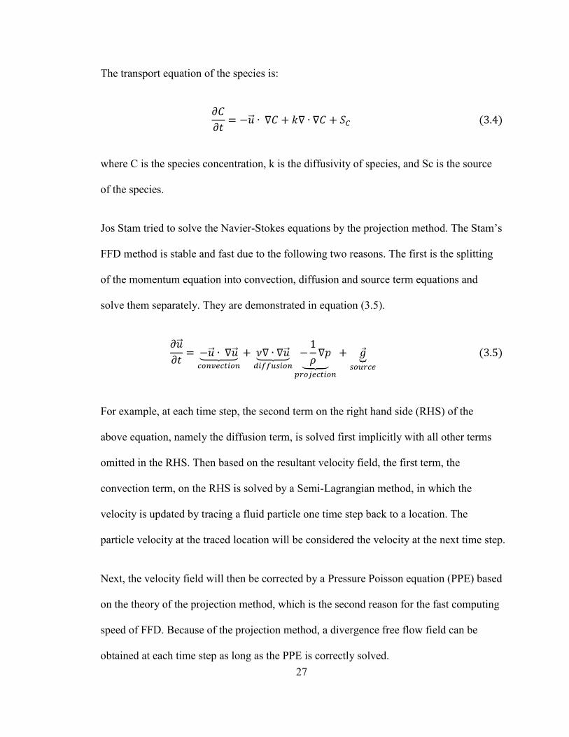
The transport equation of the species is:
where C is the species concentration, k is the diffusivity of species, and Sc is the source
of the species.
Jos Stam tried to solve the Navier-Stokes equations by the projection method. The Stam’s
FFD method is stable and fast due to the following two reasons. The first is the splitting
of the momentum equation into convection, diffusion and source term equations and
solve them separately. They are demonstrated in equation (3.5).
For example, at each time step, the second term on the right hand side (RHS) of the
above equation, namely the diffusion term, is solved first implicitly with all other terms
omitted in the RHS. Then based on the resultant velocity field, the first term, the
convection term, on the RHS is solved by a Semi-Lagrangian method, in which the
velocity is updated by tracing a fluid particle one time step back to a location. The
particle velocity at the traced location will be considered the velocity at the next time step.
Next, the velocity field will then be corrected by a Pressure Poisson equation (PPE) based
on the theory of the projection method, which is the second reason for the fast computing
speed of FFD. Because of the projection method, a divergence free flow field can be
obtained at each time step as long as the PPE is correctly solved.
28
3.1.2 Semi-Lagrangian Method
There are two basic approaches to solve the fluid motion problem. One is the Lagrangian
approach. It treats the continuum like a particle system, tracking each particle’s position
and velocity. The other one is the Eulerian approach. It uses a fixed coordinate grid
system to measure the change of each grid’s variables in time.
The Semi-Lagrangian method, which was originally proposed by Robert [55], is a
combination of the two approaches above. It calculates the trajectory of each point of the
grid to get its velocity in the previous time.
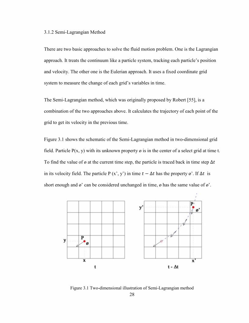
Figure 3.1 shows the schematic of the Semi-Lagrangian method in two-dimensional grid
field. Particle P(x, y) with its unknown property ø is in the center of a select grid at time t.
To find the value of ø at the current time step, the particle is traced back in time step
in its velocity field. The particle P (x’, y’) in time has the property ø’. If is
short enough and ø’ can be considered unchanged in time, ø has the same value of ø’.
Figure 3.1 Two-dimensional illustration of Semi-Lagrangian method
29
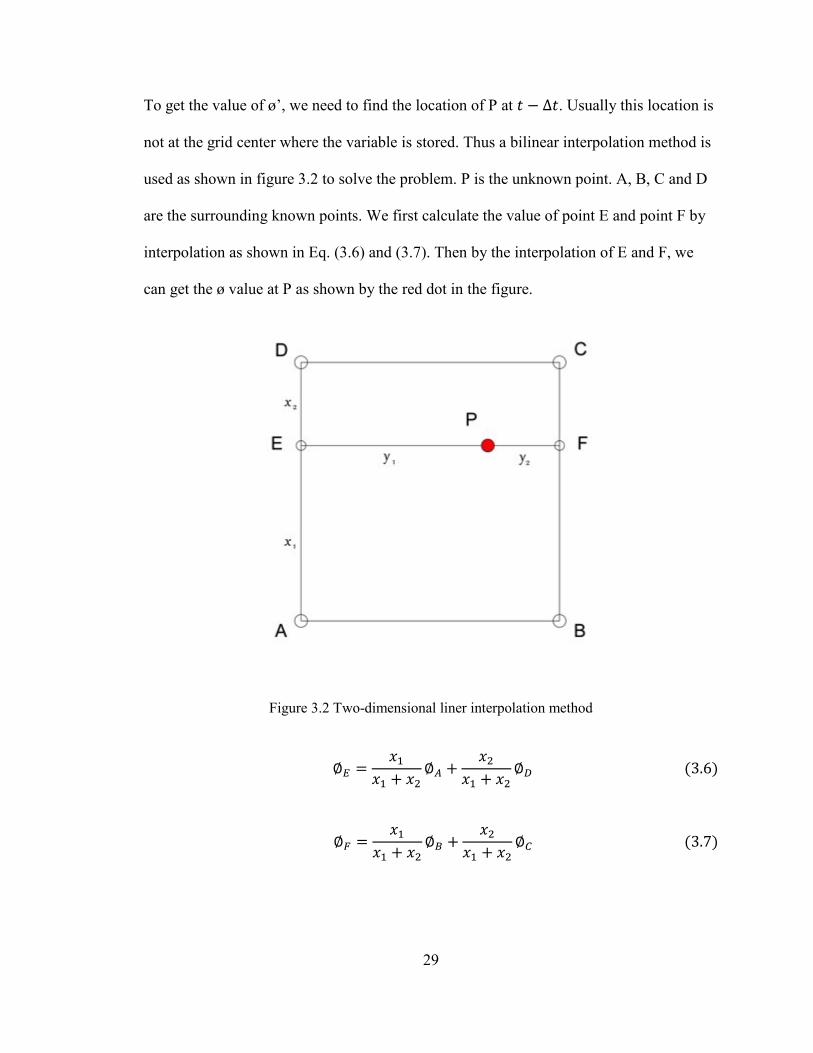
To get the value of ø’, we need to find the location of P at . Usually this location is
not at the grid center where the variable is stored. Thus a bilinear interpolation method is
used as shown in figure 3.2 to solve the problem. P is the unknown point. A, B, C and D
are the surrounding known points. We first calculate the value of point E and point F by
interpolation as shown in Eq. (3.6) and (3.7). Then by the interpolation of E and F, we
can get the ø value at P as shown by the red dot in the figure.
Figure 3.2 Two-dimensional liner interpolation method
30
Substituting Eq. (3.6) and (3.7) into Eq. (3.8), we can get
3.1.3 Zero-Equation Model for Indoor Turbulent Airflow
When the airflow is turbulent, turbulence models will be needed. The - series of
models are widely used in indoor CFD simulations, however, it is time-consuming for
solving extra - transport equations. The zero-equation model which is proposed by
Chen and Xu [56] has been used for indoor turbulent airflow simulation as below:
where is the effective viscosity of the turbulent viscosity, is the local mean velocity,
and is the length scale.
They used the model to simulate the natural convection, forced convection, mixed
convection, and displacement ventilation in a room, and compared the results with
experimental data and the results solved by - model. It has reasonable accuracy.
Meanwhile, comparing to the - models, this zero-equation model uses much less
computer memory and has at least 10 times faster of computing speed [56].
31
3.1.4 Discretization of Governing Equations
The governing equations need to be discretized to be solved numerically on each grid.
The two-dimensional momentum equation is chosen as an example. First we use the first
order time-splitting method to split the equation 3.2 into four simple equations as shown
below:
where , , are the intermediate values between the current time step value and
the next time step value . Equation (3.11) is the term of adding source, here only the
gravitational force is considered. Equation (3.12) solves the diffusion term. Equation
(3.13) is for the advection calculation. Equation (3.14) is the pressure equation, which is
solved by the projection method. Those four equations are solved sequentially and
illustrated in steps as below:
Then, we discretize the four equations. For the source term which is the equation (3.11),
32
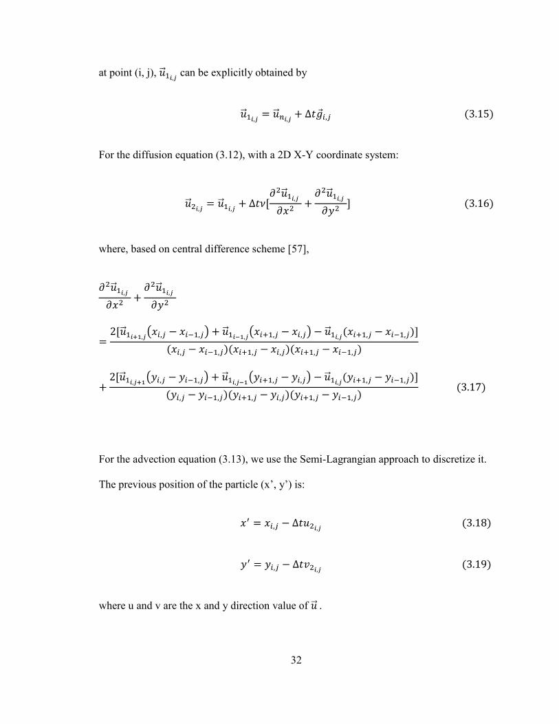
at point (i, j), can be explicitly obtained by
For the diffusion equation (3.12), with a 2D X-Y coordinate system:
where, based on central difference scheme [57],
For the advection equation (3.13), we use the Semi-Lagrangian approach to discretize it.
The previous position of the particle (x’, y’) is:
where u and v are the x and y direction value of .
33
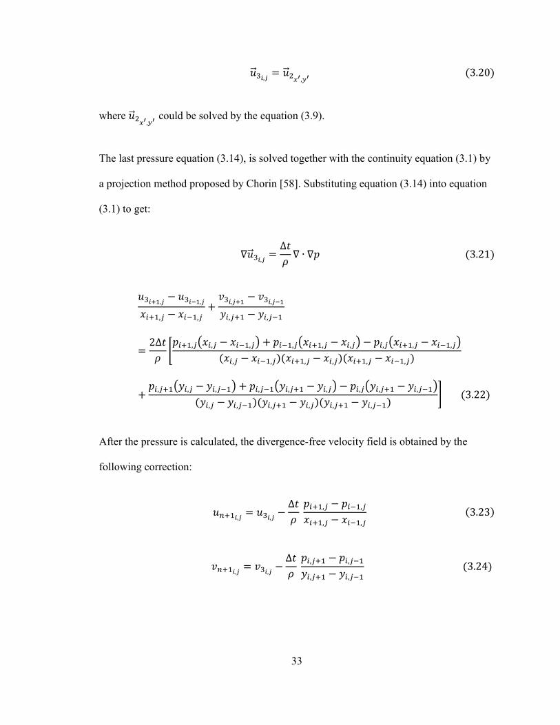
where could be solved by the equation (3.9).
The last pressure equation (3.14), is solved together with the continuity equation (3.1) by
a projection method proposed by Chorin [58]. Substituting equation (3.14) into equation
(3.1) to get:
After the pressure is calculated, the divergence-free velocity field is obtained by the
following correction:
34
3.1.5 Our Improvements on FFD
Since Stam’s FFD solver was developed for computer graphics (CG) and animations, the
method concerns more about the visual effects than the accuracy. Both the current study
and the previous studies [51] found that the divergence free field is not actually obtained
although the flow field looks to satisfy the mass balance from a visual point of view. Zuo
and Chen considered that the mass imbalance was caused by the finite difference method
and the collocated grid used in the Stam’s code. They then rewrote the code by using the
finite volume method and staggered grid, which is the traditional method as originally
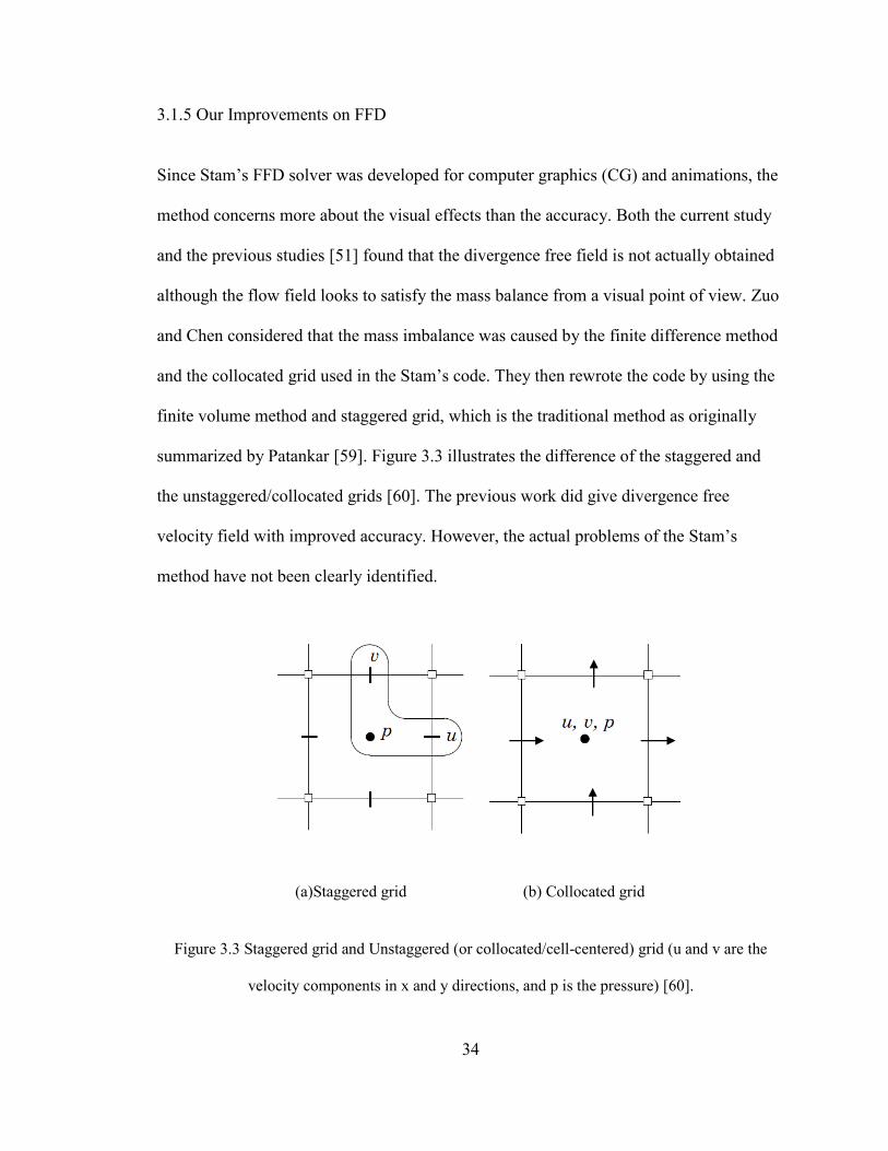
summarized by Patankar [59]. Figure 3.3 illustrates the difference of the staggered and
the unstaggered/collocated grids [60]. The previous work did give divergence free
velocity field with improved accuracy. However, the actual problems of the Stam’s
method have not been clearly identified.
(a)Staggered grid (b) Collocated grid
Figure 3.3 Staggered grid and Unstaggered (or collocated/cell-centered) grid (u and v are the
velocity components in x and y directions, and p is the pressure) [60].
35
In this study, it is found that the real problems for the mass imbalance in Stam’s method
are not the finite difference method or the collocated grid but the formulation of the
velocity divergence in the PPE and the poor performance of the linear solver (i.e. Gauss
Seidel) to solve the PPE. In the Stam’s method, the velocity divergence is evaluated from
the cell-face velocities, which are not explicitly defined but obtained from the cell-center
velocities based on the simple central differencing. After the PPE is solved, the cell-
center velocities are corrected first and then the cell-face velocities are evaluated by using
central differencing to find a new velocity divergence, which is supposed to be zero.
However, this formulation of the velocity divergence brings an extra source term so the
new velocity divergence cannot be zero even if the PPE is exactly solved.
The second cause of the mass imbalance of the Stam’s method is the poor performance of
the Gauss-Seidel (G-S) linear solver for the PPE. A close check on the convergence rate
on the G-S solver shows that for a typical 64 × 64 grid, it often takes more than 2000
sweeps of all grids to reach a convergence of 1×10⁻⁵
for the PPE at EACH time step. The
default maximum number of the G-S solver is 20 iterations which is far less than the
required iterations to reach convergence. However, the simulation will be extremely slow
if the iteration number is increased to 2000.
To fix the problem of the mass imbalance, we explicitly defined the cell-face velocities
(normal to the cell face) as shown by the four velocity arrows in Figure 3.3(b). We then
used the obtained pressure to correct the cell-face velocities directly to be used for the
calculation of the velocity divergence in the PPE. Note that compared to the staggered
grid in Figure 3.3(a), the cell-face velocities are not actually solved from the N-S
36
equations but rather obtained by two interpolation options from the cell-centered velocity:
the QUICK scheme [61], which is a higher-order upwind scheme, and the Rhie-Chow
scheme [62], which is developed for a collocated grid system and has been widely used,
such as in the commercial CFD software, ANSYS CFX [9].
Figure 3.4 The calculation structure for the full multigrid (FMG) method in the new FFD solver.
Starting on the coarsest grid, the FMG interpolates and then refines the solution onto finer grids.
E means exact solution on the coarsest grid and S means smoothing [63].
To fix the problem of low performance of the G-S solver, we implemented a new linear
solver for the PPE, a 2-D Multigrid method, based on the original code from the
Numerical Recipes [63]. Figure 3.4 shows the calculation structure for the full multigrid
method (FMG) with V-cycles of the 2-D solver. The new 2-D Multigrid solver has been
revised to handle inhomogeneous and/or Neumann boundary conditions besides the
original Derichlet boundary conditions. By the previous two efforts, the 2-D FFD code
37
can reach a convergence of 1×10⁻⁶
easily so a divergence-free velocity field is always
satisfied.
3.2. GPU on CONTAM
CONTAM is a popular multizone network model, which developed by the Indoor Air
Quality and Ventilation Group of the Engineering Laboratory at National Institute of
Standards and Technology (NIST). This study tries to port the CPU version of CONTAM
to the GPU platform to explore the potential of using GPU computing for CONTAM.
Typically, a CONTAM simulation without CFD only takes seconds or minutes so this
study will focus on the combined CFD and multizone simulations, for which over 99 %
computing time is spent by the CFD module. The first step is to analyse the performance
of CONTAM and identifying the most time-consuming functions by using the Microsoft
Visual Studio’s profiling tool. The functions are then ported to the NVIDIA CUDA GPU
platform. We demonstrate the computing speedup by comparing the running time of each
function and the whole program for the CPU and GPU versions of CONTAM in the
simulations of two cases. One case is the steady-state simulation of airflow and
contaminant transport in a five-zone office suite with a central hallway [64] and the other
is the transient simulation of contaminant transport in a single-story house [65].
The profiling capability of Microsoft Visual Studio is an important tool to evaluate and
optimize the performance of a software program. This study applies the profiling to both
the CPU and GPU codes to provide the computing time in seconds for each function. The
38
computing speedup is then defined by the ratio of the computing time on CPU over that
on GPU.
(1)
By profiling, the most time-consuming functions will be identified, which are often
expected to be those with multiple “for-loops”, especially the calculations of the
linearized coefficients of momentum equations, air and contaminant mass balance
equations, because these loops of coefficient functions are calculated for each grid point
in serial manners on CPU. Figure 3.5(a) shows a pseudo code for the CPU calculation of
three coefficient arrays, A, B and C, by a three-level for-loop. Apparently, the same
calculation is conducted for every grid point for a 3-dimensional CFD simulation.
Therefore, it will be more efficient if the calculation can be conducted simultaneously in
a parallel manner. Figure 3.5(b) illustrates how the parallel computing on a GPU is
performed. First, certain amount of memory needs to be allocated on GPU for storing the
data, copied from the regular internal memory of a PC (CPU memory) to the GPU on-
board memory. Then the parallel calculation (often called a “thread”) is run for each
element of the three arrays by one of the many GPU microprocessors. Since a GPU can
have hundreds or thousands of microprocessors, the computing time can be saved
significantly. When the calculations are finished, the results will be copied from the GPU
memory back to the CPU before the GPU memory is cleared later.
GPU
CPU
T
TSpeedup
39
(a)
(b)
Figure 3.5 The pseudo codes and structures of (a) the original CPU program and (b) its
corresponding GPU version.
Probably, Figure 3.5(b) shows one of the most straightforward applications of GPU
computing, the potential of which for speeding up scientific computing could be a lot
more than the proposed method. However, it will still be worth the effort to implement
the method to study the potential GPU speedups in such an exploratory research as the
int main ()
{
…for (k = k1; k <= k2; k++)
{
for (j = j1; j <= j2; j++)
{
for (i = i1; i <= i2; i++)
{
calculation (A[i][j][k], B[i][j][k], C[i][j][k]);
}
}
}
…
}
int main ()
{
…
cudaMalloc(cudaA, cudaB, cudaC);
…
cuda_host_to_device_copy(A, cudaA, B, cudaB, C, cudaC);
…
calculation<<<numBlocks, threadsPerBlock>>> (cudaA, cudaB,
cudaC);
…
cuda_device_to_host_copy(cudaA, A, cudaB, B, cudaC, C);
…
cudaFree(cudaA, cudaB, cudaC);
…
}
Main program
Memory allocation on GPU
Copy data from CPU to GPU
Parallel calculation of each
element of A, B, C arrays on
GPU Copy data from GPU to CPU
Free GPU memory
End Program
Main program
Loop for grid index k
Loop for grid index j
Loop for grid index i
Serial calculation of A, B, C
arrays End loop for i
End loop for j
End loop for k
End program
40
current study.
3.3. SketchUp Plug-in
As part of the current work, it is very important to develop a graphical interface to create
the geometrical models for FFD simulations. A user-friendly tool could reduce the
operating time and attract users’ interest to use the tool. SketchUp [66] was chosen to be
the platform to develop such an interface tool. It is currently widely used because the
SketchUp operation is very straightforward that people could draw a 3D object in
seconds without any previous professional CAD training. It is also affordable and it could
be freely downloaded. The developers are encouraged to write plug-ins for it using the
powerful the Ruby language.
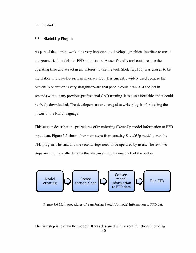
This section describes the procedures of transferring SketchUp model information to FFD
input data. Figure 3.3 shows four main steps from creating SketchUp model to run the
FFD plug-in. The first and the second steps need to be operated by users. The rest two
steps are automatically done by the plug-in simply by one click of the button.
Figure 3.6 Main procedures of transferring SketchUp model information to FFD data.
The first step is to draw the models. It was designed with several functions including
Model creating
Create section plane
Convert model
information to FFD data
Run FFD
41
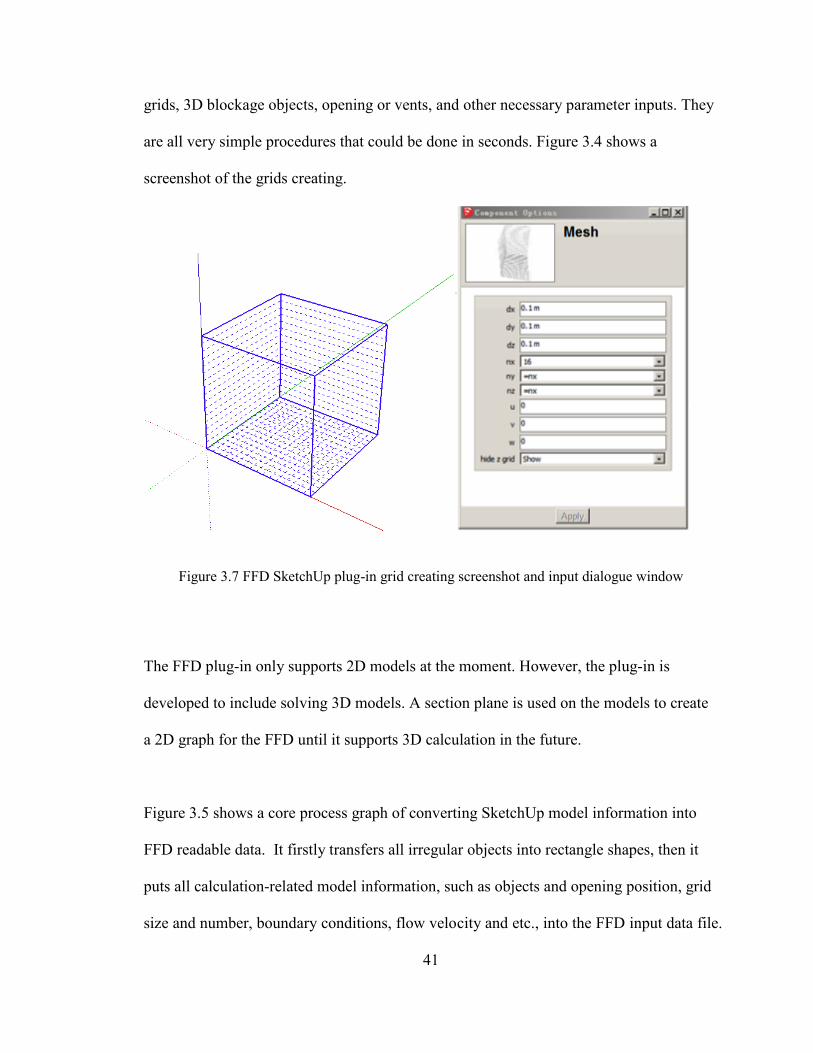
grids, 3D blockage objects, opening or vents, and other necessary parameter inputs. They
are all very simple procedures that could be done in seconds. Figure 3.4 shows a
screenshot of the grids creating.
Figure 3.7 FFD SketchUp plug-in grid creating screenshot and input dialogue window
The FFD plug-in only supports 2D models at the moment. However, the plug-in is
developed to include solving 3D models. A section plane is used on the models to create
a 2D graph for the FFD until it supports 3D calculation in the future.
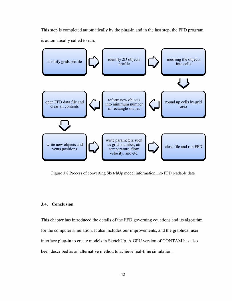
Figure 3.5 shows a core process graph of converting SketchUp model information into
FFD readable data. It firstly transfers all irregular objects into rectangle shapes, then it
puts all calculation-related model information, such as objects and opening position, grid
size and number, boundary conditions, flow velocity and etc., into the FFD input data file.
42
This step is completed automatically by the plug-in and in the last step, the FFD program
is automatically called to run.
Figure 3.8 Process of converting SketchUp model information into FFD readable data
3.4. Conclusion
This chapter has introduced the details of the FFD governing equations and its algorithm
for the computer simulation. It also includes our improvements, and the graphical user
interface plug-in to create models in SketchUp. A GPU version of CONTAM has also
been described as an alternative method to achieve real-time simulation.
identify grids profile identify 2D objects
profile meshing the objects
into cells
round up cells by grid area
reform new objects into minimum number
of rectangle shapes
open FFD data file and clear all contents
write new objects and vents positions
write parameters such as grids number, air temperature, flow velocity, and etc.
close file and run FFD
43
CHAPTER 4. RESULTS AND DISCUSSION
4.1. Comparison of CONTAM on GPU and on CPU
To evaluate the performance of CONTAM developed on GPU, two cases in the literature
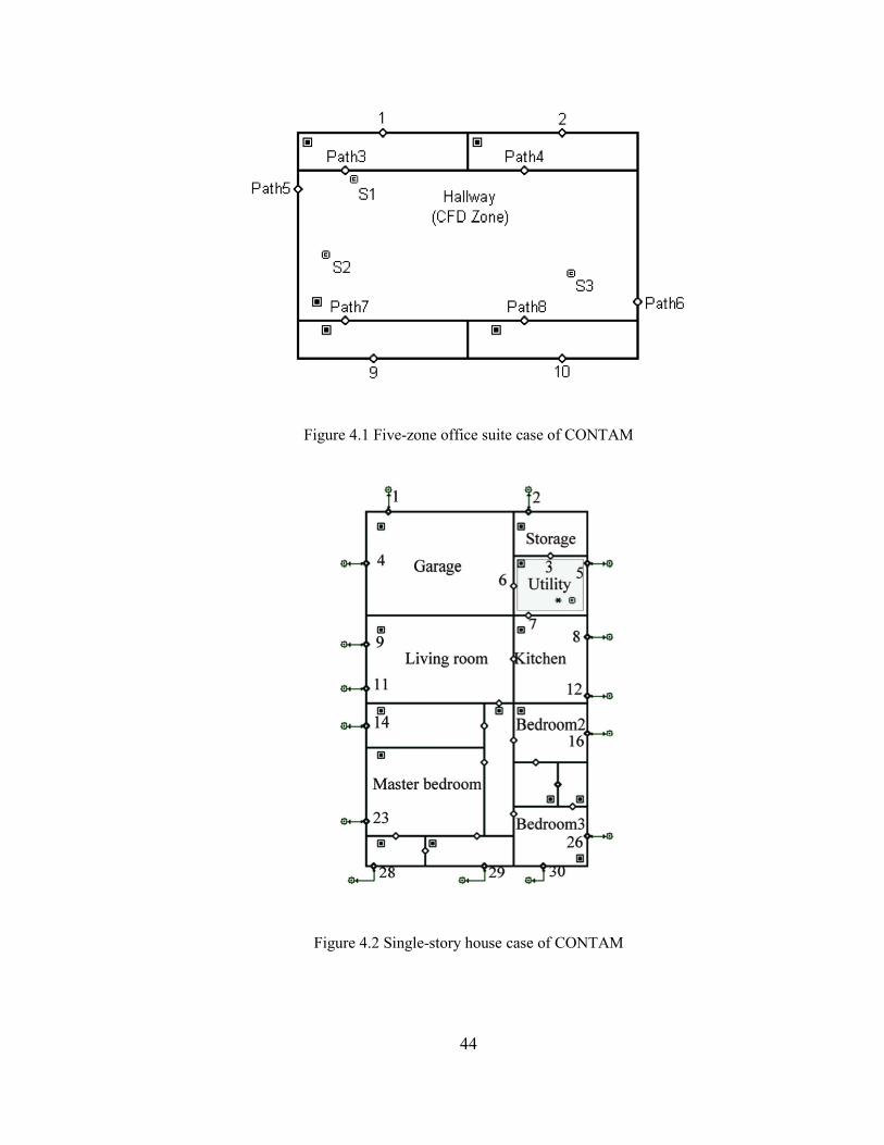
are selected to compare to the CPU simulations for this study. The first case is the five-
zone office suite with a hallway in the center and two office rooms on each side [64]. A
wind-driven airflow through the front door of the hallway is modeled in steady state. Two
gaseous contaminant sources with constant release rates are placed at different locations
in the hallway. Because both the airflow and contaminant transport in the hallway
invalidate the well-mixed assumption, the hallway is selected to be simulated by the CFD
and the rest of the rooms by the network model. The details of the case setup can be
found from the CONTAM 3.0 tutorial published on the NIST CONTAM website [64].
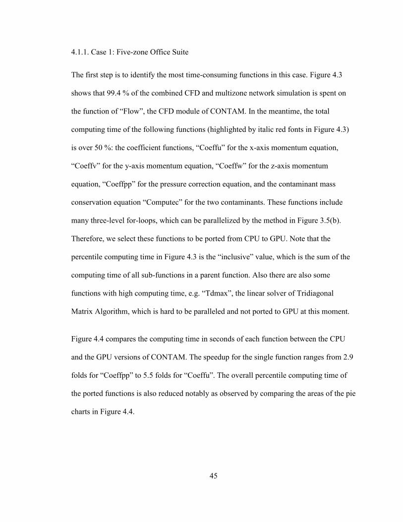
The other case is the one-story single family house, where the gas furnace in the utility
room is assumed malfunctioning and releasing carbon monoxide (CO) [65]. The utility
room is thus simulated by the CFD, and the remaining rooms are simulated as well-mixed
zones by the network model.
Both cases used the same computer configuration: the CPU is Intel® Xeon® Processor
W3503 with 2.4 GHz clockspeed and 2 Cores, the Graphics card is NVIDIA Quadro
4000 with 256 CUDA Cores and 486.4 Gigaflops (Single Precision).
44
Figure 4.1 Five-zone office suite case of CONTAM
Figure 4.2 Single-story house case of CONTAM
45
4.1.1. Case 1: Five-zone Office Suite
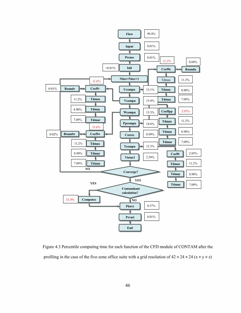
The first step is to identify the most time-consuming functions in this case. Figure 4.3
shows that 99.4 % of the combined CFD and multizone network simulation is spent on
the function of “Flow”, the CFD module of CONTAM. In the meantime, the total
computing time of the following functions (highlighted by italic red fonts in Figure 4.3)
is over 50 %: the coefficient functions, “Coeffu” for the x-axis momentum equation,
“Coeffv” for the y-axis momentum equation, “Coeffw” for the z-axis momentum
equation, “Coeffpp” for the pressure correction equation, and the contaminant mass
conservation equation “Computec” for the two contaminants. These functions include
many three-level for-loops, which can be parallelized by the method in Figure 3.5(b).
Therefore, we select these functions to be ported from CPU to GPU. Note that the
percentile computing time in Figure 4.3 is the “inclusive” value, which is the sum of the
computing time of all sub-functions in a parent function. Also there are also some
functions with high computing time, e.g. “Tdmax”, the linear solver of Tridiagonal
Matrix Algorithm, which is hard to be paralleled and not ported to GPU at this moment.
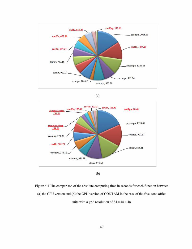
Figure 4.4 compares the computing time in seconds of each function between the CPU
and the GPU versions of CONTAM. The speedup for the single function ranges from 2.9
folds for “Coeffpp” to 5.5 folds for “Coeffu”. The overall percentile computing time of
the ported functions is also reduced notably as observed by comparing the areas of the pie
charts in Figure 4.4.
46
Figure 4.3 Percentile computing time for each function of the CFD module of CONTAM after the
profiling in the case of the five-zone office suite with a grid resolution of 42 × 24 × 24 (x × y × z)
NO
YES
NO
YES
Flow
Input
Prcase
Init
Niter=Niter+1
Ucompu
Vcompu
Wcompu
Ppcompu
Correc
Tcompu
Vistur1
Converge?
Plotvt
Prvari
Coeffu
Tdmax
Tdmay
Tdmaz
Boundu
Coeffv
Tdmax
Tdmay
Tdmaz
Boundv
Coeffw
Tdmax
Tdmay
Tdmaz
Boundw
Coeffpp
Tdmax
Tdmay
Tdmaz
Coefft
Tdmax
Tdmay
Tdmaz
Contaminant
calculation?
Computec
End
0.01%
0.01%
15.1%
15.4%
0.01
15.3%
18.6%
11.3%
4
0.04%
0.01%
11.6%
2.05%
11.6%
0.02%
11.2%
3
11.2%
3
11.2%
3
11.2%
3
8.90%
8.90%
8.90%
8.90%
8.90%
7.09%
7.09%
7.09%
7.09%
7.09%
11.2%
3
2.05%
0.99%
2.59%
99.4%
31.5%
0.57%
0.01%
<0.01%
12.3%
47
(a)
(b)
Figure 4.4 The comparison of the absolute computing time in seconds for each function between
(a) the CPU version and (b) the GPU version of CONTAM in the case of the five-zone office
suite with a grid resolution of 84 × 48 × 48.
48
Meanwhile, there are computing overheads during the porting, e.g. the operations of
converting between double precision and single precision numbers because the current
GPU cards are more efficient to handle single precisions than double ones as illustrated
by Figure 4.3. Table 4.1 shows that the overhead caused by precision conversions is
about 13.9 % for the coarse grid and 9.1 % for the fine grid. The overhead cost can be
possibly reduced in the future study when the GPU manufacturers improve their double
precision calculations.
Due to the overhead, the total speedup of the GPU computing in the case of five-zone
office suite is about 1.9 folds for the grid resolution of 84 × 48 × 48 and 1.5 folds for the
grid of 42 × 24 × 24 as illustrated in Table 4.1. It is thus shown that more computing
speedup can be achieved when the grid resolution is increased. Therefore, data-intensive
and parallelizable CFD calculations will benefit well from GPU computing.
4.1.2. Case 2: Single-story House
In the previous case, the airflow and contaminant transport are simulated at steady state,
so the ported coefficient functions share a similar order of computing time for the given
grid resolution. For the single-story house in this section, we firstly calculate the airflow
at steady state, based on which the transient transport of CO in the house is then
calculated for two hours with a time step of one minute, i.e. the calculation of CO mass
conservation equation is repeated for 120 times.
49
Table 4.1 Comparison of the total computing time of the CPU and GPU versions of CONTAM.
Grids
(x × y × z)
CPU Time
(minutes)
GPU Time
(minutes)
Speedup
(CPU/GPU)
Overhead/Total Time
(due to single & double
precision conversion)
Five-zone office suite
42 × 24 × 24 4.0 2.7 1.5 13.9 %
84 × 48 × 48 106.0 58.0 1.9 9.1 %
Single-story house
70 × 70 × 90 403.1 66.4 6.1 5.6 %
Table 4.1 shows that the total computing time of the GPU code is about 66.4 minutes,
which is equivalently a speedup of 6.1 folds. Therefore, repetitive calculations of the
same functions, e.g. in a transient simulation, will also benefit well from the parallel
capability of the GPU computing.
(a)
50
(b)
Figure 4.5 The comparison of the absolute computing time in seconds for each function between
(a) the CPU version and (b) the GPU version of CONTAM in the case of the single-story house
with a grid resolution of 70 × 70 × 90.
When comparing the computing time for a single function, we find more speedups as
shown in Figure 4.5. The speedup ranges from 10.8 folds for “Coeffc” to 22.5 for
“Coeffu”, which are significantly higher than those in the previous case. The speedup
improvement can be attributed to the smaller overhead from the precision conversion,
which is only 5.6 % of the total running time (Table 4.1). Therefore, the reduction of the
overheads of GPU computing contributes well to the speedup. Meanwhile, for the two
cases modeled in this study, it is found that the difference of the results of the CPU and
GPU simulations is negligible. The comparison of the results is not included here for
simplicity. The conversion of single and double precisions thus did not cause accuracy
problems in this study.
51
4.1.3. Conclusion
This study explores the potential of using GPU computing to speed up the CFD module
in CONTAM by porting multi-level “for-loops” on CPU to parallel calculations on GPU.
It was found that the best GPU speedup could be 6.1 folds of the total computing time
and 22.5 folds for a single function. The GPU computing will well benefit the data-
intensive simulation, where the grid resolution is high, and the transient calculation,
where the associated function is repeatedly calculated for many times. It was also found
that the GPU speedup could be further improved by reducing the overheads of porting to
GPU, e.g. conversion of single and double precisions. It was noted that the speedup of 6.1
folds by GPU is not impressive considering the huge speedup in the literature of using the
new algorithms, e.g. fast fluid dynamics (FFD). Therefore, further optimization and/or
the application of FFD is needed in order to achieve real-time or faster-than-real-time
simulations.
4.2. FFD Real-time Simulation Results
This section demonstrates how to achieve real-time simulations by the FFD algorithms
investigated in this thesis. A two-dimensional flow over a cylinder case is demonstrated
to show the FFD simulation results. Flow over a circular cylinder is a classical problem in
fluid mechanics for the complex unsteady dynamics of the cylinder wake flow. A famous
phenomenon called von Kármán vortex street will occur during the change of Reynolds
number. Figure 4.6 is a photo of vortex street in the wake of Selkirk Island, which is
taken in September 1999 by the Landsat 7 satellite [67].
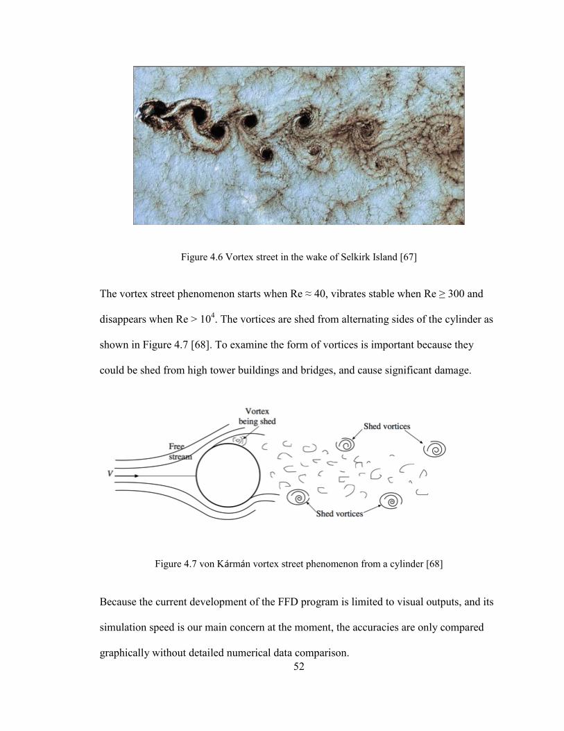
52
Figure 4.6 Vortex street in the wake of Selkirk Island [67]
The vortex street phenomenon starts when Re ≈ 40, vibrates stable when Re ≥ 300 and
disappears when Re > 104. The vortices are shed from alternating sides of the cylinder as
shown in Figure 4.7 [68]. To examine the form of vortices is important because they
could be shed from high tower buildings and bridges, and cause significant damage.
Figure 4.7 von Kármán vortex street phenomenon from a cylinder [68]
Because the current development of the FFD program is limited to visual outputs, and its
simulation speed is our main concern at the moment, the accuracies are only compared
graphically without detailed numerical data comparison.
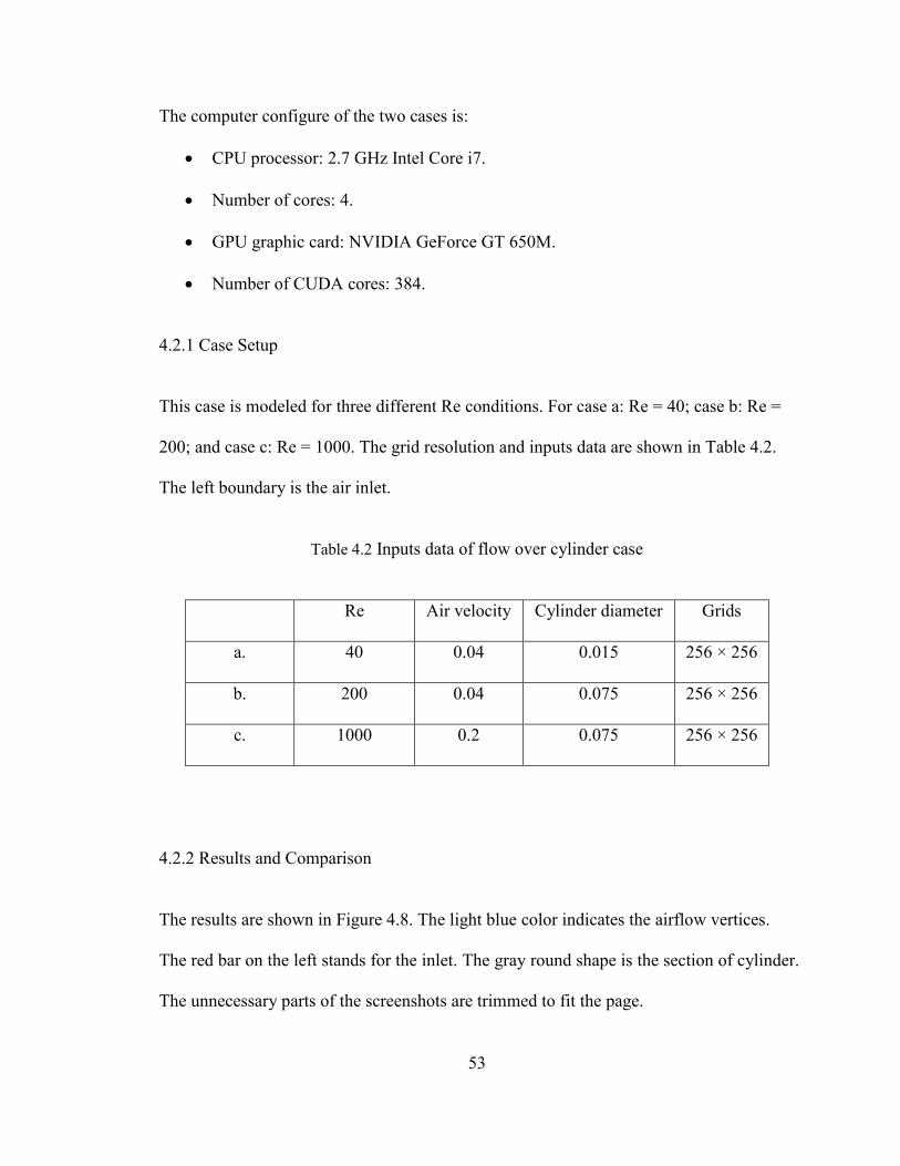
53
The computer configure of the two cases is:
CPU processor: 2.7 GHz Intel Core i7.
Number of cores: 4.
GPU graphic card: NVIDIA GeForce GT 650M.
Number of CUDA cores: 384.
4.2.1 Case Setup
This case is modeled for three different Re conditions. For case a: Re = 40; case b: Re =
200; and case c: Re = 1000. The grid resolution and inputs data are shown in Table 4.2.
The left boundary is the air inlet.
Table 4.2 Inputs data of flow over cylinder case
Re Air velocity Cylinder diameter Grids
a. 40 0.04 0.015 256 × 256
b. 200 0.04 0.075 256 × 256
c. 1000 0.2 0.075 256 × 256
4.2.2 Results and Comparison
The results are shown in Figure 4.8. The light blue color indicates the airflow vertices.
The red bar on the left stands for the inlet. The gray round shape is the section of cylinder.
The unnecessary parts of the screenshots are trimmed to fit the page.
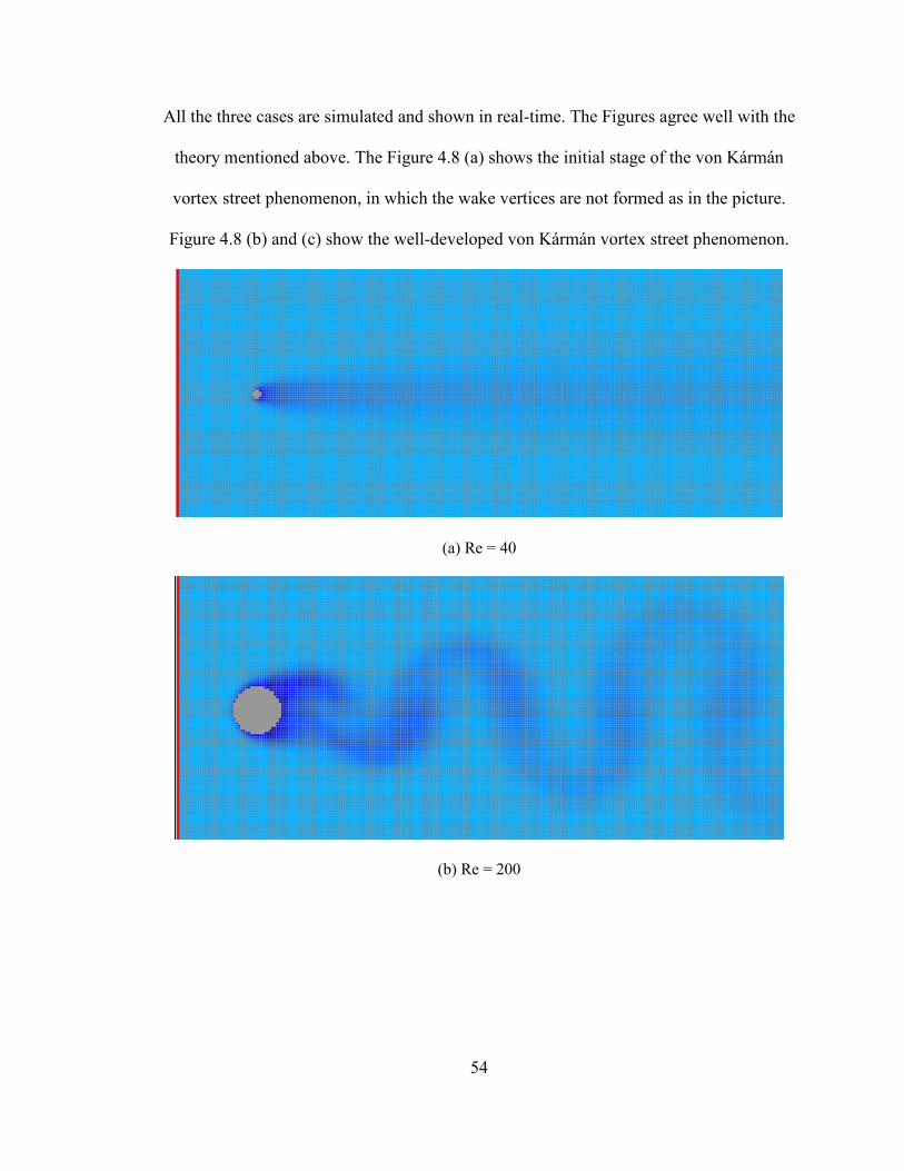
54
All the three cases are simulated and shown in real-time. The Figures agree well with the
theory mentioned above. The Figure 4.8 (a) shows the initial stage of the von Kármán
vortex street phenomenon, in which the wake vertices are not formed as in the picture.
Figure 4.8 (b) and (c) show the well-developed von Kármán vortex street phenomenon.
(a) Re = 40
(b) Re = 200
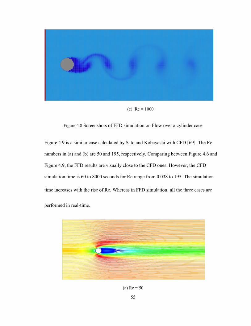
55
(c) Re = 1000
Figure 4.8 Screenshots of FFD simulation on Flow over a cylinder case
Figure 4.9 is a similar case calculated by Sato and Kobayashi with CFD [69]. The Re
numbers in (a) and (b) are 50 and 195, respectively. Comparing between Figure 4.6 and
Figure 4.9, the FFD results are visually close to the CFD ones. However, the CFD
simulation time is 60 to 8000 seconds for Re range from 0.038 to 195. The simulation
time increases with the rise of Re. Whereas in FFD simulation, all the three cases are
performed in real-time.
(a) Re = 50
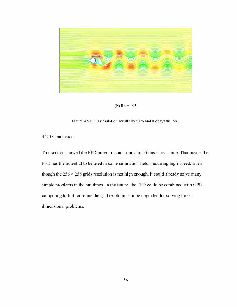
56
(b) Re = 195
Figure 4.9 CFD simulation results by Sato and Kobayashi [69].
4.2.3 Conclusion
This section showed the FFD program could run simulations in real-time. That means the
FFD has the potential to be used in some simulation fields requiring high-speed. Even
though the 256 × 256 grids resolution is not high enough, it could already solve many
simple problems in the buildings. In the future, the FFD could be combined with GPU
computing to further refine the grid resolutions or be upgraded for solving three-
dimensional problems.
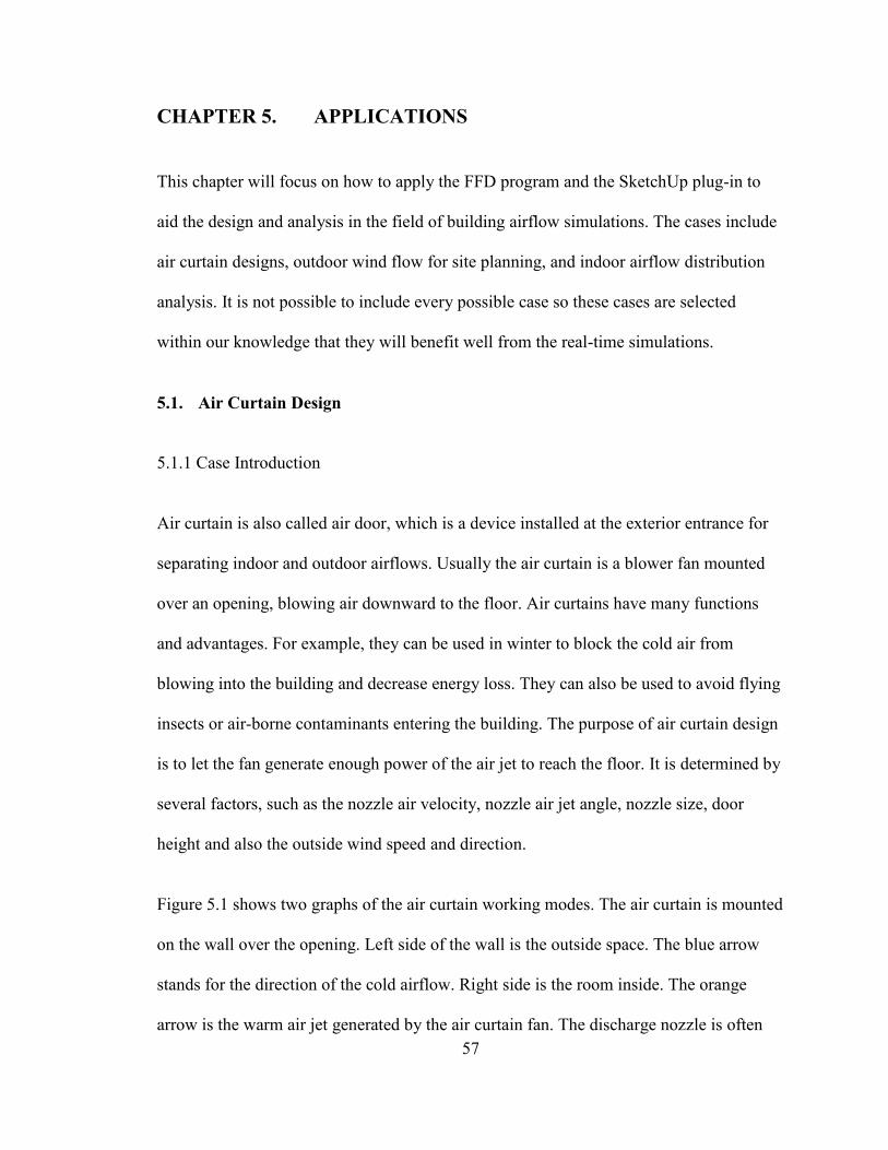
57
CHAPTER 5. APPLICATIONS
This chapter will focus on how to apply the FFD program and the SketchUp plug-in to
aid the design and analysis in the field of building airflow simulations. The cases include
air curtain designs, outdoor wind flow for site planning, and indoor airflow distribution
analysis. It is not possible to include every possible case so these cases are selected
within our knowledge that they will benefit well from the real-time simulations.
5.1. Air Curtain Design
5.1.1 Case Introduction
Air curtain is also called air door, which is a device installed at the exterior entrance for
separating indoor and outdoor airflows. Usually the air curtain is a blower fan mounted
over an opening, blowing air downward to the floor. Air curtains have many functions
and advantages. For example, they can be used in winter to block the cold air from
blowing into the building and decrease energy loss. They can also be used to avoid flying
insects or air-borne contaminants entering the building. The purpose of air curtain design
is to let the fan generate enough power of the air jet to reach the floor. It is determined by
several factors, such as the nozzle air velocity, nozzle air jet angle, nozzle size, door
height and also the outside wind speed and direction.
Figure 5.1 shows two graphs of the air curtain working modes. The air curtain is mounted
on the wall over the opening. Left side of the wall is the outside space. The blue arrow
stands for the direction of the cold airflow. Right side is the room inside. The orange
arrow is the warm air jet generated by the air curtain fan. The discharge nozzle is often
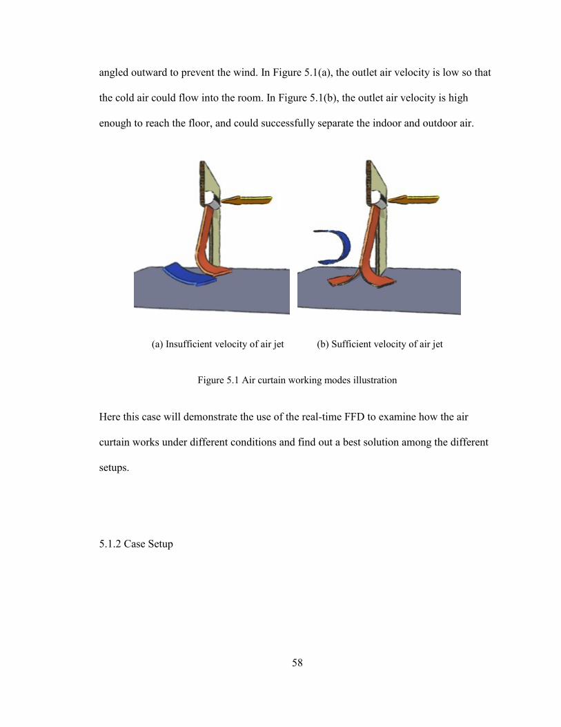
58
angled outward to prevent the wind. In Figure 5.1(a), the outlet air velocity is low so that
the cold air could flow into the room. In Figure 5.1(b), the outlet air velocity is high
enough to reach the floor, and could successfully separate the indoor and outdoor air.
(a) Insufficient velocity of air jet (b) Sufficient velocity of air jet
Figure 5.1 Air curtain working modes illustration
Here this case will demonstrate the use of the real-time FFD to examine how the air
curtain works under different conditions and find out a best solution among the different
setups.
5.1.2 Case Setup
59
Figure 5.2 Sketch of 2D Air curtain case
Figure 5.2 demonstrates the sketch of the case. Wind blows from outdoor to indoor
direction horizontally. The air curtain nozzle generates high-speed air jet with a vertical
angle θ against the wind direction as shown in Figure 5.2. The airflow circulates out from
the right boundary. The floor keeps a distance from the left and right side of the boundary
to give the airflow an alternative pathway. If the air curtain fails to generate enough jet to
block the wind, the wind will mix with the indoor air and follow the path above the floor
(red arrows) to circulate out. Otherwise, the wind will circulate out beneath the floor
(blue arrows).
In this case, the FFD will simulate the air circulation in different situations to see the
performance of the air curtain. Three different nozzle angle θ will be compared firstly. A
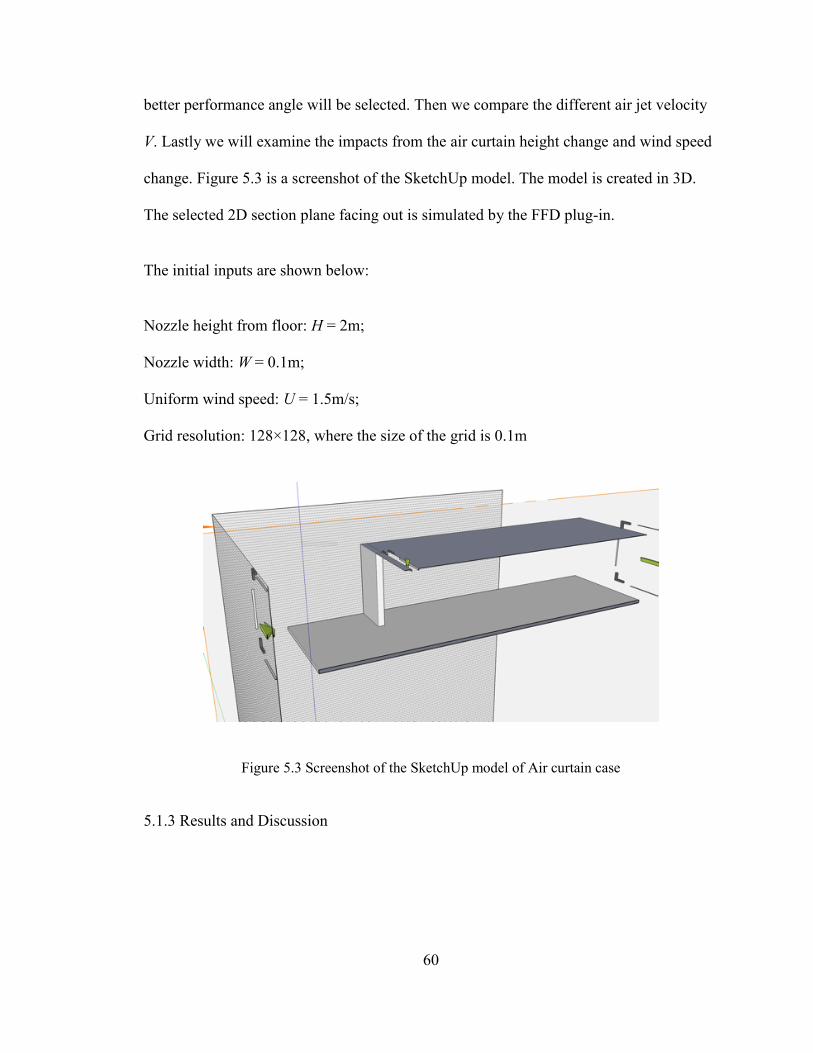
60
better performance angle will be selected. Then we compare the different air jet velocity
V. Lastly we will examine the impacts from the air curtain height change and wind speed
change. Figure 5.3 is a screenshot of the SketchUp model. The model is created in 3D.
The selected 2D section plane facing out is simulated by the FFD plug-in.
The initial inputs are shown below:
Nozzle height from floor: H = 2m;
Nozzle width: W = 0.1m;
Uniform wind speed: U = 1.5m/s;
Grid resolution: 128×128, where the size of the grid is 0.1m
Figure 5.3 Screenshot of the SketchUp model of Air curtain case
5.1.3 Results and Discussion
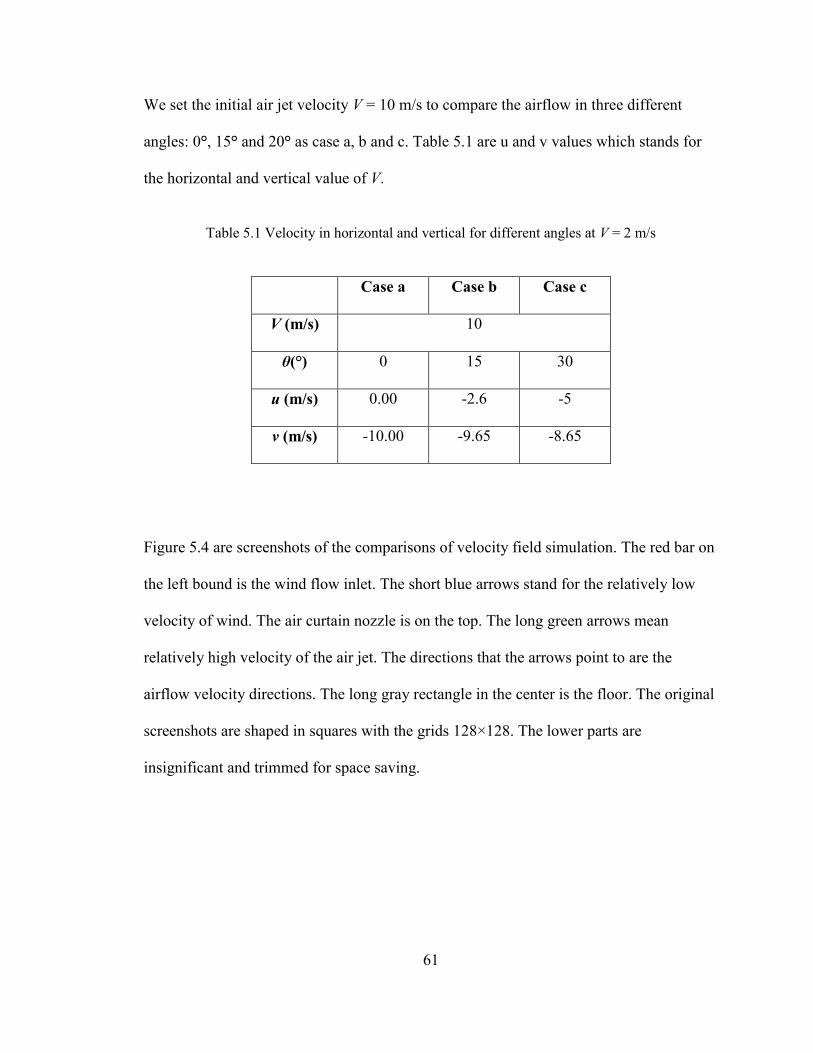
61
We set the initial air jet velocity V = 10 m/s to compare the airflow in three different
angles: 0°, 15° and 20° as case a, b and c. Table 5.1 are u and v values which stands for
the horizontal and vertical value of V.
Table 5.1 Velocity in horizontal and vertical for different angles at V = 2 m/s
Case a Case b Case c
V (m/s) 10
θ(°) 0 15 30
u (m/s) 0.00 -2.6 -5
v (m/s) -10.00 -9.65 -8.65
Figure 5.4 are screenshots of the comparisons of velocity field simulation. The red bar on
the left bound is the wind flow inlet. The short blue arrows stand for the relatively low
velocity of wind. The air curtain nozzle is on the top. The long green arrows mean
relatively high velocity of the air jet. The directions that the arrows point to are the
airflow velocity directions. The long gray rectangle in the center is the floor. The original
screenshots are shaped in squares with the grids 128×128. The lower parts are
insignificant and trimmed for space saving.
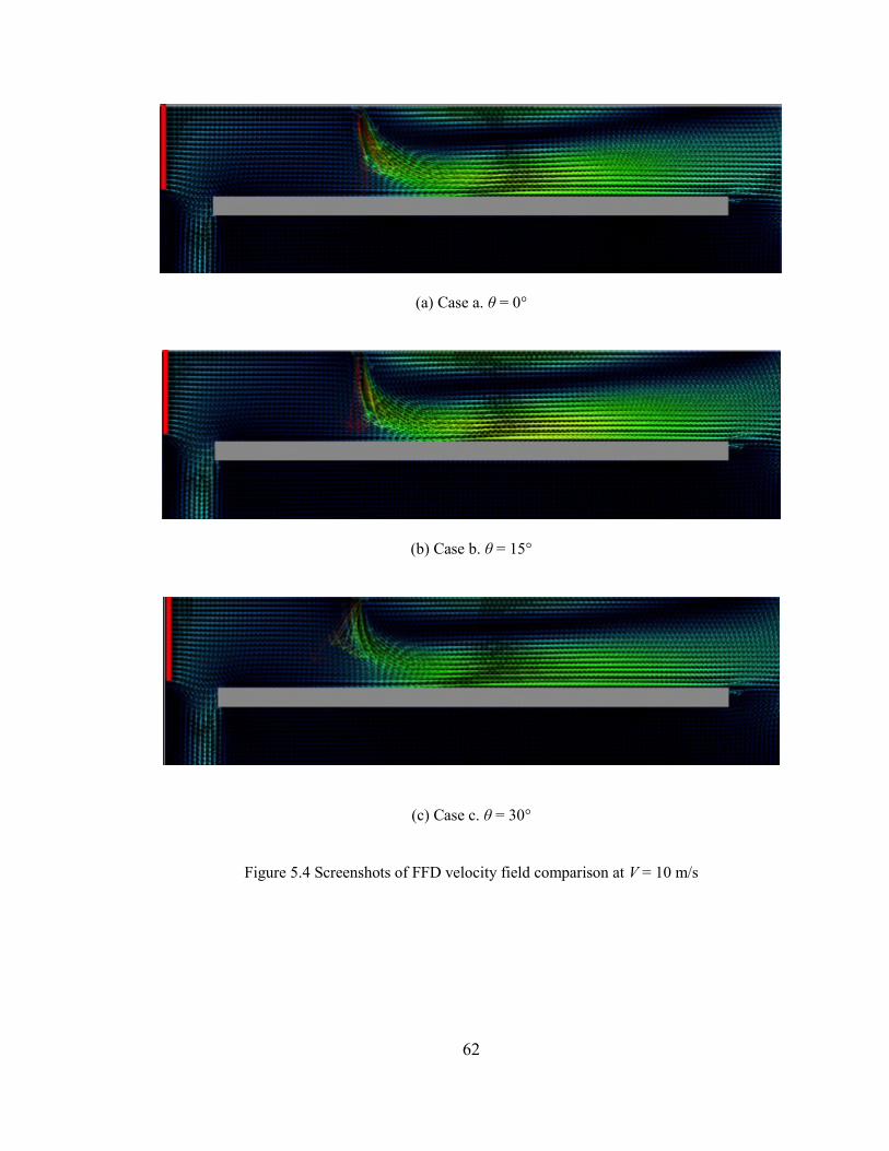
62
(a) Case a. θ = 0°
(b) Case b. θ = 15°
(c) Case c. θ = 30°
Figure 5.4 Screenshots of FFD velocity field comparison at V = 10 m/s
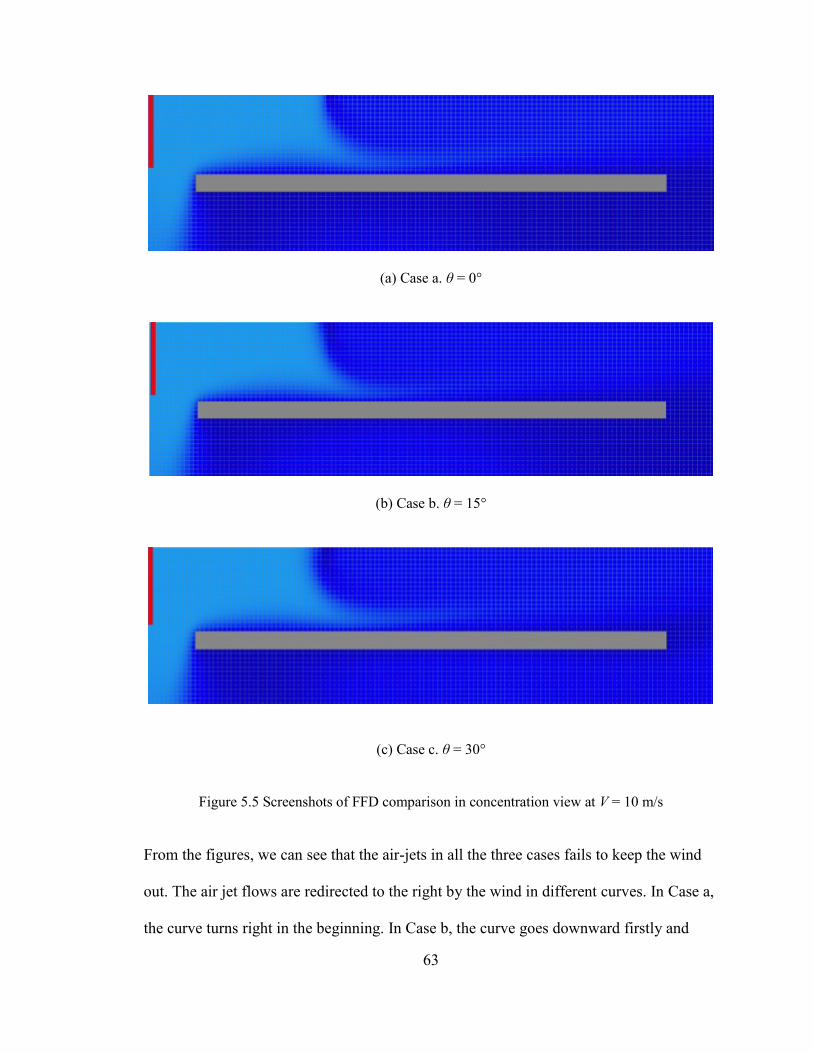
63
(a) Case a. θ = 0°
(b) Case b. θ = 15°
(c) Case c. θ = 30°
Figure 5.5 Screenshots of FFD comparison in concentration view at V = 10 m/s
From the figures, we can see that the air-jets in all the three cases fails to keep the wind
out. The air jet flows are redirected to the right by the wind in different curves. In Case a,
the curve turns right in the beginning. In Case b, the curve goes downward firstly and
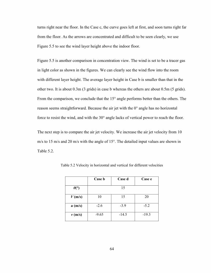
64
turns right near the floor. In the Case c, the curve goes left at first, and soon turns right far
from the floor. As the arrows are concentrated and difficult to be seen clearly, we use
Figure 5.5 to see the wind layer height above the indoor floor.
Figure 5.5 is another comparison in concentration view. The wind is set to be a tracer gas
in light color as shown in the figures. We can clearly see the wind flow into the room
with different layer height. The average layer height in Case b is smaller than that in the
other two. It is about 0.3m (3 grids) in case b whereas the others are about 0.5m (5 grids).
From the comparison, we conclude that the 15° angle performs better than the others. The
reason seems straightforward. Because the air jet with the 0° angle has no horizontal
force to resist the wind, and with the 30° angle lacks of vertical power to reach the floor.
The next step is to compare the air jet velocity. We increase the air jet velocity from 10
m/s to 15 m/s and 20 m/s with the angle of 15°. The detailed input values are shown in
Table 5.2.
Table 5.2 Velocity in horizontal and vertical for different velocities
Case b Case d Case e
θ(°) 15
V (m/s) 10 15 20
u (m/s) -2.6 -3.9 -5.2
v (m/s) -9.65 -14.5 -19.3
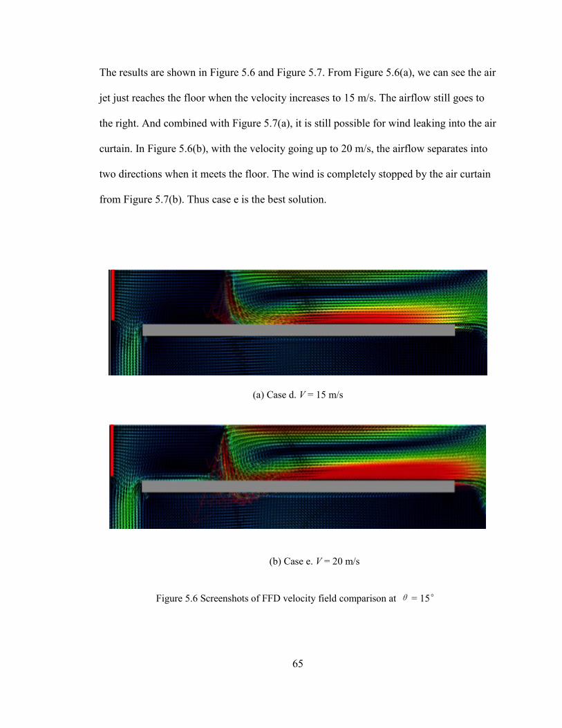
65
The results are shown in Figure 5.6 and Figure 5.7. From Figure 5.6(a), we can see the air
jet just reaches the floor when the velocity increases to 15 m/s. The airflow still goes to
the right. And combined with Figure 5.7(a), it is still possible for wind leaking into the air
curtain. In Figure 5.6(b), with the velocity going up to 20 m/s, the airflow separates into
two directions when it meets the floor. The wind is completely stopped by the air curtain
from Figure 5.7(b). Thus case e is the best solution.
(a) Case d. V = 15 m/s
(b) Case e. V = 20 m/s
Figure 5.6 Screenshots of FFD velocity field comparison at θ = 15°
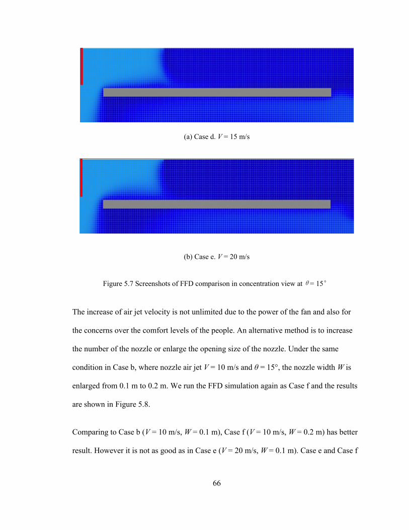
66
(a) Case d. V = 15 m/s
(b) Case e. V = 20 m/s
Figure 5.7 Screenshots of FFD comparison in concentration view atθ= 15°
The increase of air jet velocity is not unlimited due to the power of the fan and also for
the concerns over the comfort levels of the people. An alternative method is to increase
the number of the nozzle or enlarge the opening size of the nozzle. Under the same
condition in Case b, where nozzle air jet V = 10 m/s and θ = 15°, the nozzle width W is
enlarged from 0.1 m to 0.2 m. We run the FFD simulation again as Case f and the results
are shown in Figure 5.8.
Comparing to Case b (V = 10 m/s, W = 0.1 m), Case f (V = 10 m/s, W = 0.2 m) has better
result. However it is not as good as in Case e (V = 20 m/s, W = 0.1 m). Case e and Case f
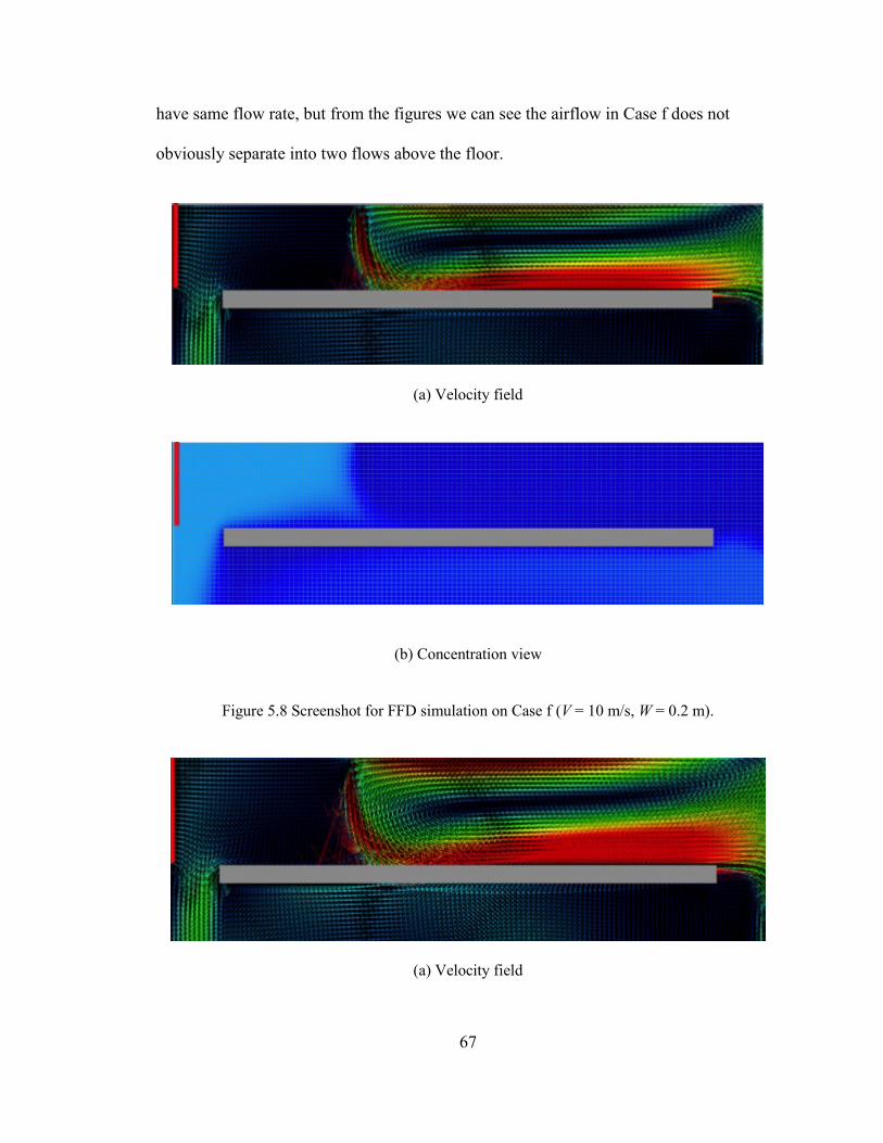
67
have same flow rate, but from the figures we can see the airflow in Case f does not
obviously separate into two flows above the floor.
(a) Velocity field
(b) Concentration view
Figure 5.8 Screenshot for FFD simulation on Case f (V = 10 m/s, W = 0.2 m).
(a) Velocity field
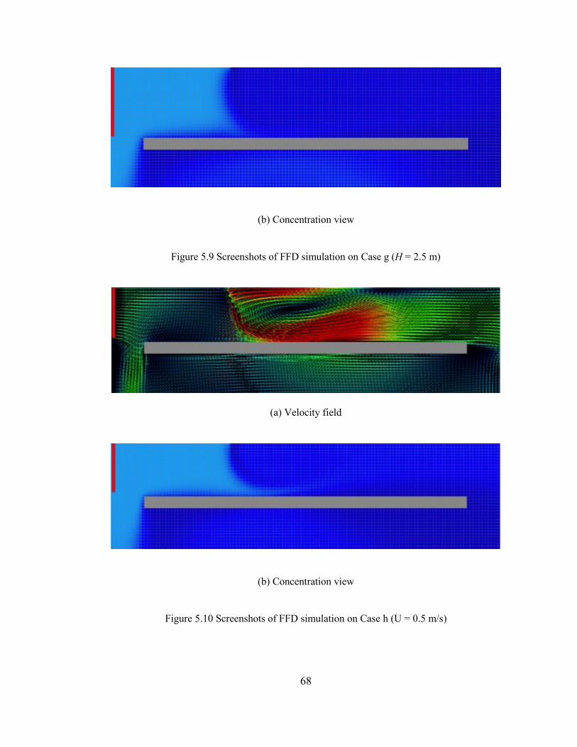
68
(b) Concentration view
Figure 5.9 Screenshots of FFD simulation on Case g (H = 2.5 m)
(a) Velocity field
(b) Concentration view
Figure 5.10 Screenshots of FFD simulation on Case h (U = 0.5 m/s)
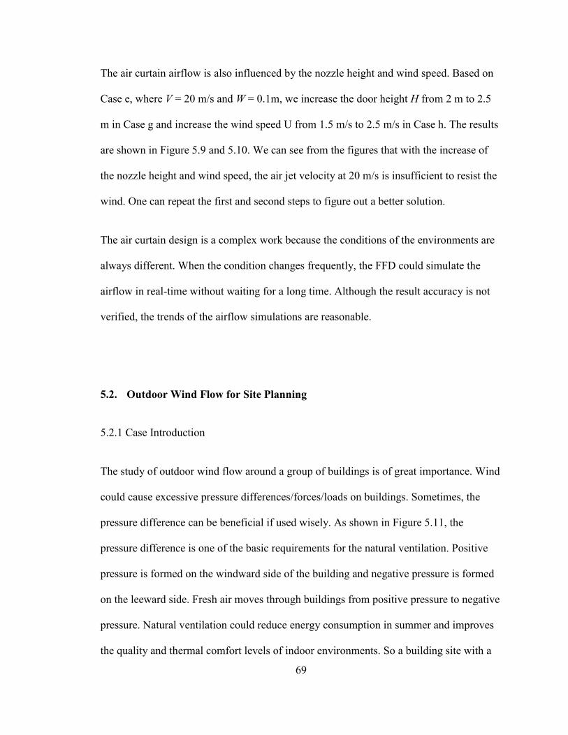
69
The air curtain airflow is also influenced by the nozzle height and wind speed. Based on
Case e, where V = 20 m/s and W = 0.1m, we increase the door height H from 2 m to 2.5
m in Case g and increase the wind speed U from 1.5 m/s to 2.5 m/s in Case h. The results
are shown in Figure 5.9 and 5.10. We can see from the figures that with the increase of
the nozzle height and wind speed, the air jet velocity at 20 m/s is insufficient to resist the
wind. One can repeat the first and second steps to figure out a better solution.
The air curtain design is a complex work because the conditions of the environments are
always different. When the condition changes frequently, the FFD could simulate the
airflow in real-time without waiting for a long time. Although the result accuracy is not
verified, the trends of the airflow simulations are reasonable.
5.2. Outdoor Wind Flow for Site Planning
5.2.1 Case Introduction
The study of outdoor wind flow around a group of buildings is of great importance. Wind
could cause excessive pressure differences/forces/loads on buildings. Sometimes, the
pressure difference can be beneficial if used wisely. As shown in Figure 5.11, the
pressure difference is one of the basic requirements for the natural ventilation. Positive
pressure is formed on the windward side of the building and negative pressure is formed
on the leeward side. Fresh air moves through buildings from positive pressure to negative
pressure. Natural ventilation could reduce energy consumption in summer and improves
the quality and thermal comfort levels of indoor environments. So a building site with a
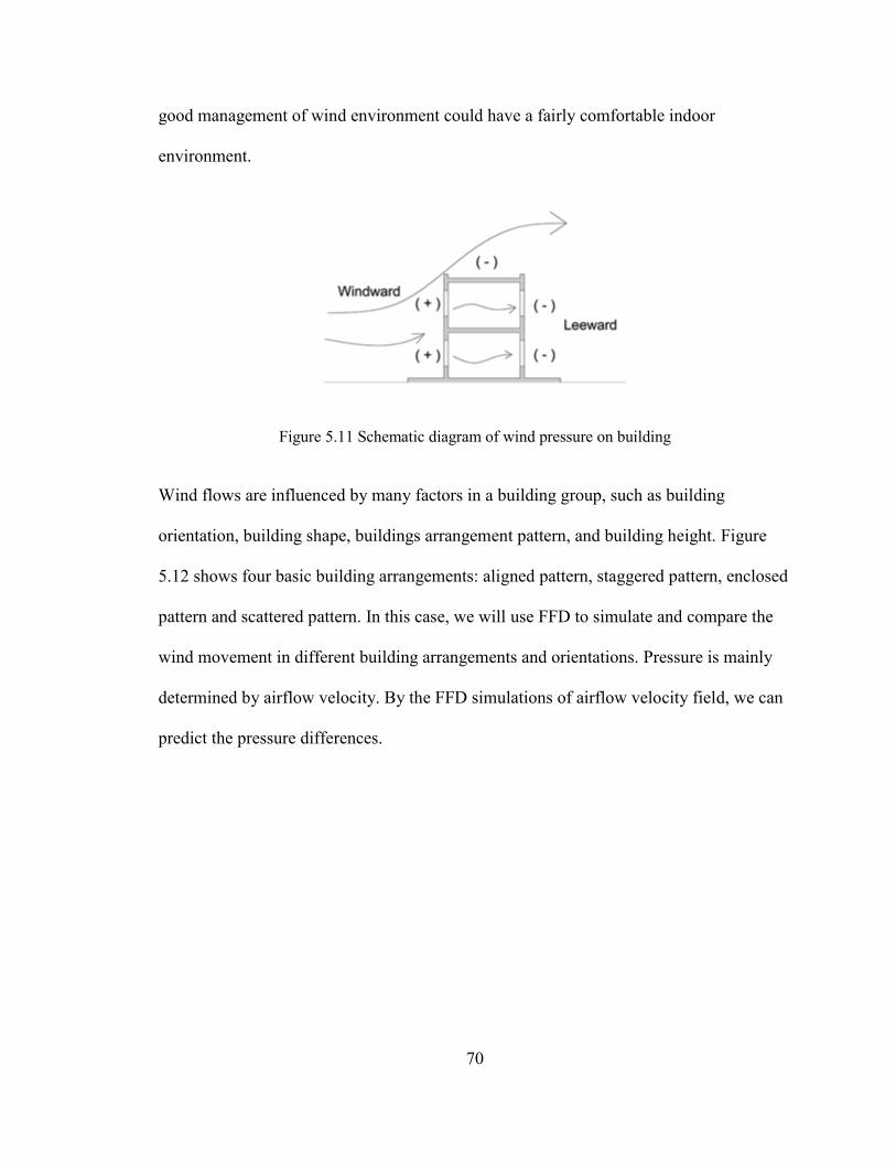
70
good management of wind environment could have a fairly comfortable indoor
environment.
Figure 5.11 Schematic diagram of wind pressure on building
Wind flows are influenced by many factors in a building group, such as building
orientation, building shape, buildings arrangement pattern, and building height. Figure
5.12 shows four basic building arrangements: aligned pattern, staggered pattern, enclosed
pattern and scattered pattern. In this case, we will use FFD to simulate and compare the
wind movement in different building arrangements and orientations. Pressure is mainly
determined by airflow velocity. By the FFD simulations of airflow velocity field, we can
predict the pressure differences.
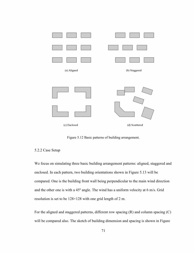
71
Figure 5.12 Basic patterns of building arrangement.
5.2.2 Case Setup
We focus on simulating three basic building arrangement patterns: aligned, staggered and
enclosed. In each pattern, two building orientations shown in Figure 5.13 will be
compared. One is the building front wall being perpendicular to the main wind direction
and the other one is with a 45º angle. The wind has a uniform velocity at 6 m/s. Grid
resolution is set to be 128×128 with one grid length of 2 m.
For the aligned and staggered patterns, different row spacing (R) and column spacing (C)
will be compared also. The sketch of building dimension and spacing is shown in Figure
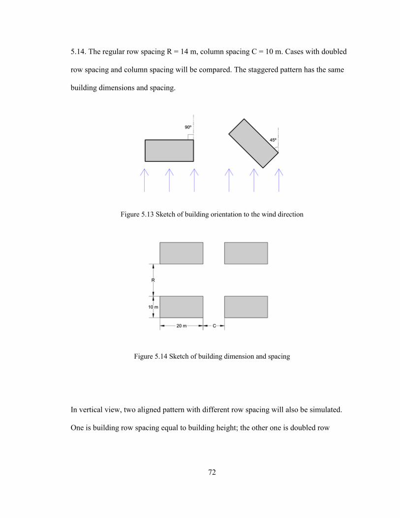
72
5.14. The regular row spacing R = 14 m, column spacing C = 10 m. Cases with doubled
row spacing and column spacing will be compared. The staggered pattern has the same
building dimensions and spacing.
Figure 5.13 Sketch of building orientation to the wind direction
Figure 5.14 Sketch of building dimension and spacing
In vertical view, two aligned pattern with different row spacing will also be simulated.
One is building row spacing equal to building height; the other one is doubled row
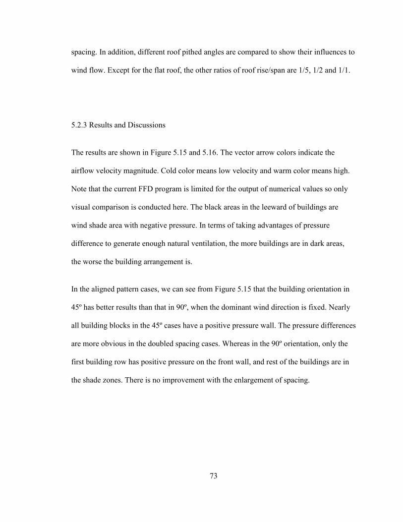
73
spacing. In addition, different roof pithed angles are compared to show their influences to
wind flow. Except for the flat roof, the other ratios of roof rise/span are 1/5, 1/2 and 1/1.
5.2.3 Results and Discussions
The results are shown in Figure 5.15 and 5.16. The vector arrow colors indicate the
airflow velocity magnitude. Cold color means low velocity and warm color means high.
Note that the current FFD program is limited for the output of numerical values so only
visual comparison is conducted here. The black areas in the leeward of buildings are
wind shade area with negative pressure. In terms of taking advantages of pressure
difference to generate enough natural ventilation, the more buildings are in dark areas,
the worse the building arrangement is.
In the aligned pattern cases, we can see from Figure 5.15 that the building orientation in
45º has better results than that in 90º, when the dominant wind direction is fixed. Nearly
all building blocks in the 45º cases have a positive pressure wall. The pressure differences
are more obvious in the doubled spacing cases. Whereas in the 90º orientation, only the
first building row has positive pressure on the front wall, and rest of the buildings are in
the shade zones. There is no improvement with the enlargement of spacing.
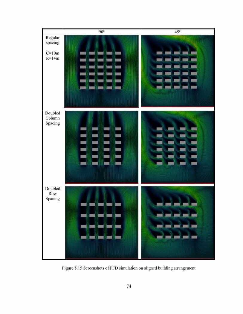
74
90º 45º
Regular
spacing
C=10m
R=14m
Doubled
Column
Spacing
Doubled
Row
Spacing
Figure 5.15 Screenshots of FFD simulation on aligned building arrangement
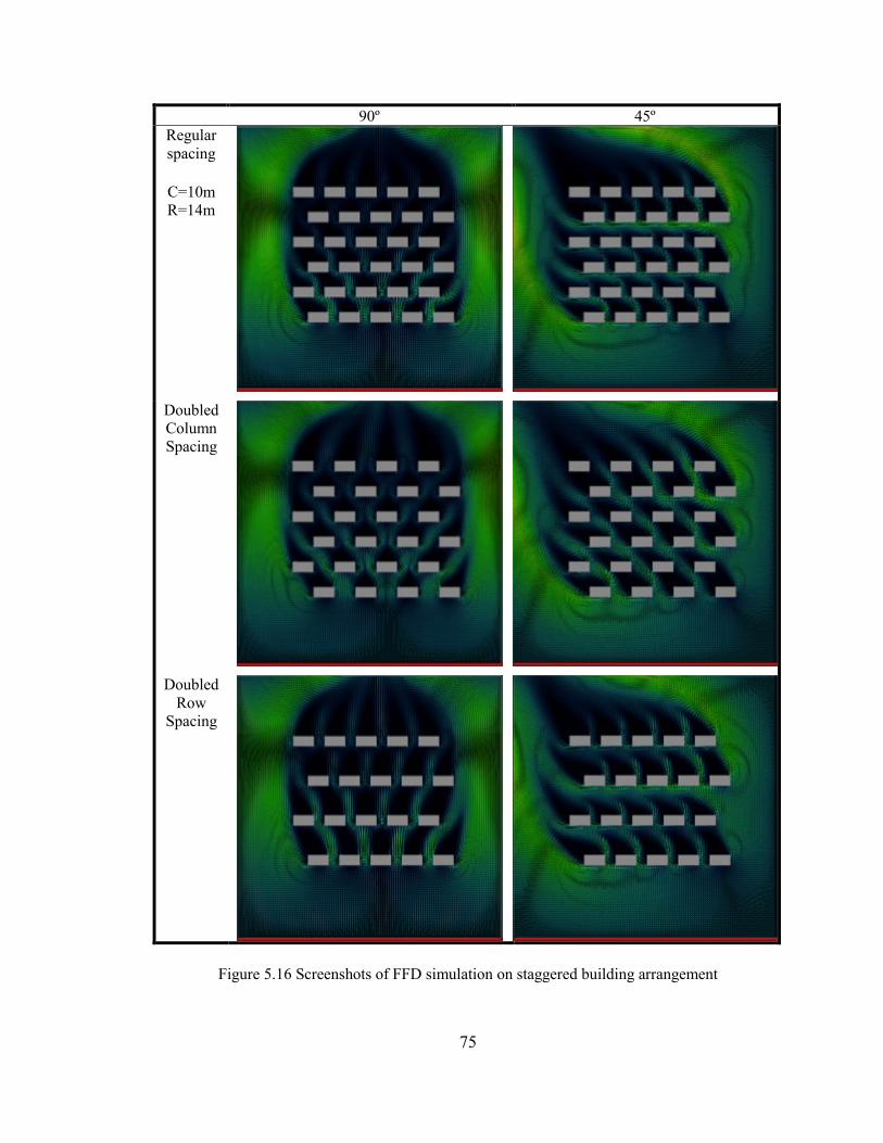
75
90º 45º
Regular
spacing
C=10m
R=14m
Doubled
Column
Spacing
Doubled
Row
Spacing
Figure 5.16 Screenshots of FFD simulation on staggered building arrangement
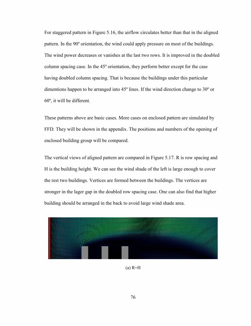
76
For staggered pattern in Figure 5.16, the airflow circulates better than that in the aligned
pattern. In the 90º orientation, the wind could apply pressure on most of the buildings.
The wind power decreases or vanishes at the last two rows. It is improved in the doubled
column spacing case. In the 45º orientation, they perform better except for the case
having doubled column spacing. That is because the buildings under this particular
dimentions happen to be arranged into 45º lines. If the wind direction change to 30º or
60º, it will be different.
These patterns above are basic cases. More cases on enclosed pattern are simulated by
FFD. They will be shown in the appendix. The positions and numbers of the opening of
enclosed building group will be compared.
The vertical views of aligned pattern are compared in Figure 5.17. R is row spacing and
H is the building height. We can see the wind shade of the left is large enough to cover
the rest two buildings. Vertices are formed between the buildings. The vertices are
stronger in the lager gap in the doubled row spacing case. One can also find that higher
building should be arranged in the back to avoid large wind shade area.
(a) R=H
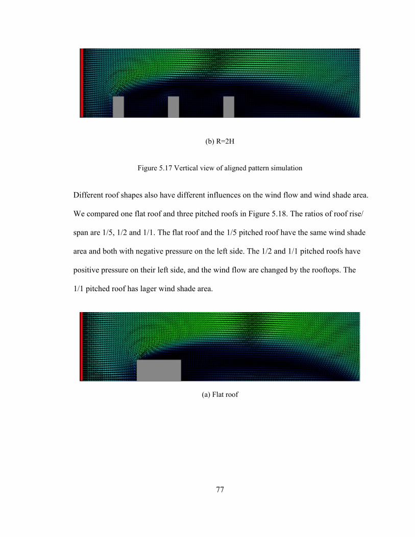
77
(b) R=2H
Figure 5.17 Vertical view of aligned pattern simulation
Different roof shapes also have different influences on the wind flow and wind shade area.
We compared one flat roof and three pitched roofs in Figure 5.18. The ratios of roof rise/
span are 1/5, 1/2 and 1/1. The flat roof and the 1/5 pitched roof have the same wind shade
area and both with negative pressure on the left side. The 1/2 and 1/1 pitched roofs have
positive pressure on their left side, and the wind flow are changed by the rooftops. The
1/1 pitched roof has lager wind shade area.
(a) Flat roof
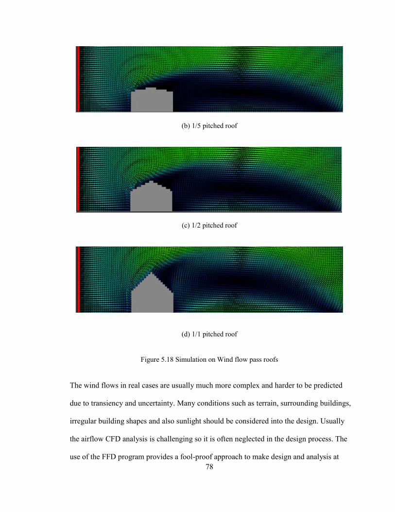
78
(b) 1/5 pitched roof
(c) 1/2 pitched roof
(d) 1/1 pitched roof
Figure 5.18 Simulation on Wind flow pass roofs
The wind flows in real cases are usually much more complex and harder to be predicted
due to transiency and uncertainty. Many conditions such as terrain, surrounding buildings,
irregular building shapes and also sunlight should be considered into the design. Usually
the airflow CFD analysis is challenging so it is often neglected in the design process. The
use of the FFD program provides a fool-proof approach to make design and analysis at
79
real time possible. The intrinsic stability of FFD simulations make it much easier to
achieve stable solutions for almost all simulations so it is also a fool-proof tool for the
users at all levels.
5.3. Indoor Airflow Distribution Analysis
5.3.1 Case Introduction
Building airflow is formed by pressure difference; the difference is caused by natural
wind, mechanical ventilation such as fans and air-conditioning, and stack effect
(buoyancy). As mentioned in previous sections and chapters, ventilation is necessary and
important in thermal comfort and health. Good airflow circulation could enhance the
ventilation efficiency and save energy. Thus controlling airflow is of significant
importance in building ventilation designs.
To form airflow, a continuous flow path between two points with pressure differences is
another prerequisite. In the previous application, we introduced the method of designing
buildings in outdoor site planning to obtain pressure differences. In this application, the
different pathways of airflow will be compared by FFD. There are two factors considered
here to determine the flow path: vent positions and partition wall locations. They will be
compared in the following simulations.
5.3.2 Case Setup
A squared room in 2D with different opening positions is selected as shown in Figure
5.19. Air is supplied into the room via one of the inlets at the west (left) wall, and
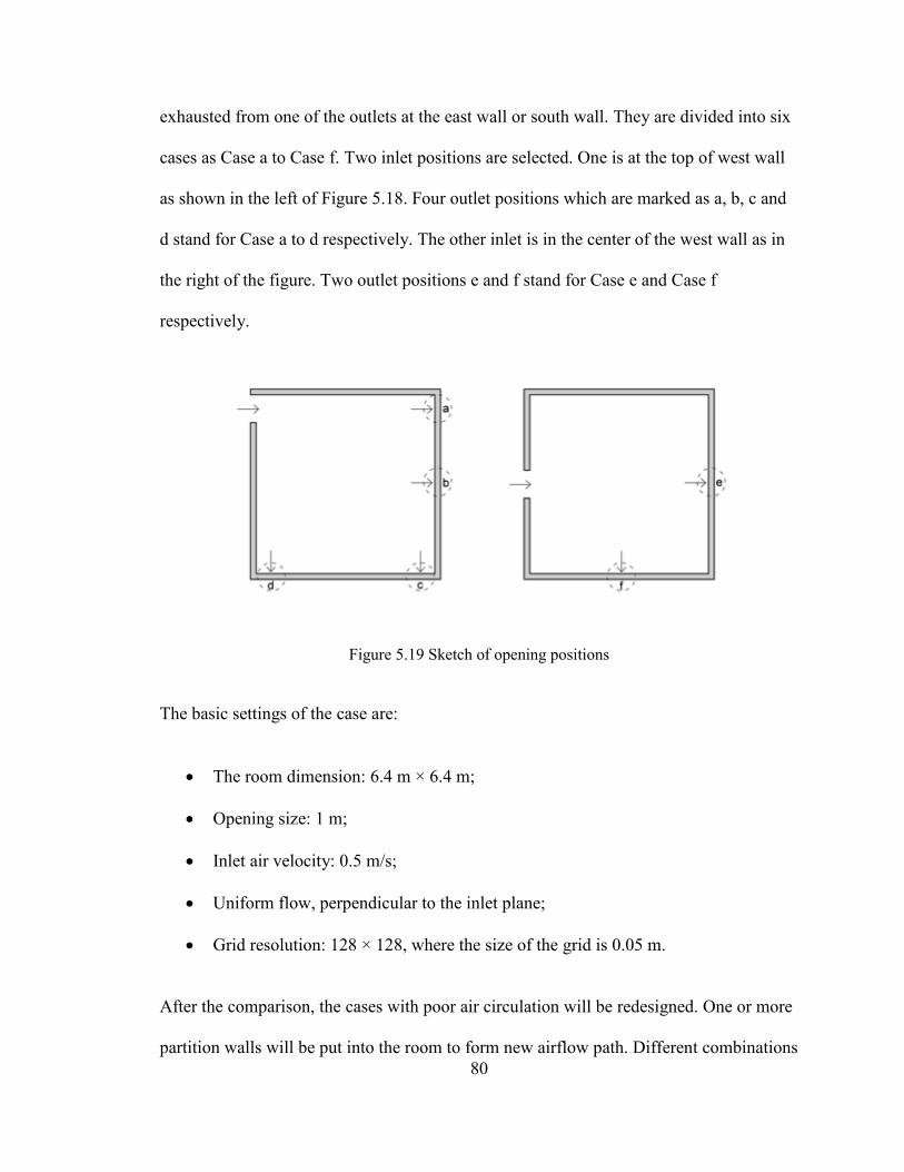
80
exhausted from one of the outlets at the east wall or south wall. They are divided into six
cases as Case a to Case f. Two inlet positions are selected. One is at the top of west wall
as shown in the left of Figure 5.18. Four outlet positions which are marked as a, b, c and
d stand for Case a to d respectively. The other inlet is in the center of the west wall as in
the right of the figure. Two outlet positions e and f stand for Case e and Case f
respectively.
Figure 5.19 Sketch of opening positions
The basic settings of the case are:
The room dimension: 6.4 m × 6.4 m;
Opening size: 1 m;
Inlet air velocity: 0.5 m/s;
Uniform flow, perpendicular to the inlet plane;
Grid resolution: 128 × 128, where the size of the grid is 0.05 m.
After the comparison, the cases with poor air circulation will be redesigned. One or more
partition walls will be put into the room to form new airflow path. Different combinations
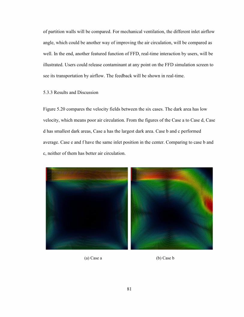
81
of partition walls will be compared. For mechanical ventilation, the different inlet airflow
angle, which could be another way of improving the air circulation, will be compared as
well. In the end, another featured function of FFD, real-time interaction by users, will be
illustrated. Users could release contaminant at any point on the FFD simulation screen to
see its transportation by airflow. The feedback will be shown in real-time.
5.3.3 Results and Discussion
Figure 5.20 compares the velocity fields between the six cases. The dark area has low
velocity, which means poor air circulation. From the figures of the Case a to Case d, Case
d has smallest dark areas, Case a has the largest dark area. Case b and c performed
average. Case e and f have the same inlet position in the center. Comparing to case b and
c, neither of them has better air circulation.
(a) Case a (b) Case b
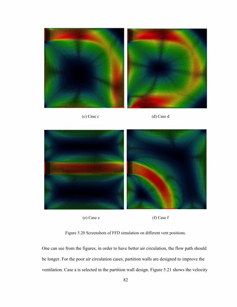
82
(c) Case c (d) Case d
(e) Case e (f) Case f
Figure 5.20 Screenshots of FFD simulation on different vent positions.
One can see from the figures, in order to have better air circulation, the flow path should
be longer. For the poor air circulation cases, partition walls are designed to improve the
ventilation. Case a is selected in the partition wall design. Figure 5.21 shows the velocity
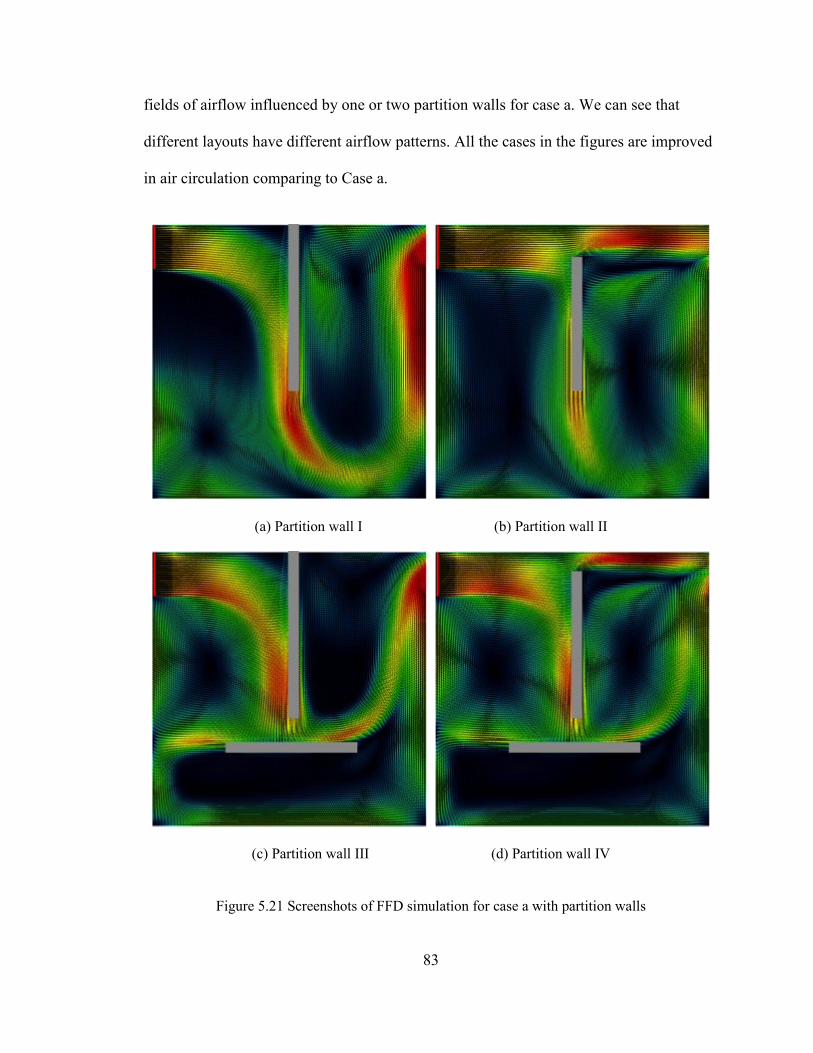
83
fields of airflow influenced by one or two partition walls for case a. We can see that
different layouts have different airflow patterns. All the cases in the figures are improved
in air circulation comparing to Case a.
(a) Partition wall I (b) Partition wall II
(c) Partition wall III (d) Partition wall IV
Figure 5.21 Screenshots of FFD simulation for case a with partition walls
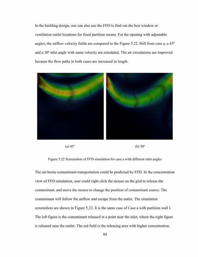
84
In the building design, one can also use the FFD to find out the best window or
ventilation outlet locations for fixed partition rooms. For the opening with adjustable
angles, the airflow velocity fields are compared in the Figure 5.22. Still from case a, a 45º
and a 30º inlet angle with same velocity are simulated. The air circulations are improved
because the flow paths in both cases are increased in length.
(a) 45º (b) 30º
Figure 5.22 Screenshots of FFD simulation for case a with different inlet angles
The air-borne contaminant transportation could be predicted by FFD. In the concentration
view of FFD simulation, user could right click the mouse on the gird to release the
contaminant, and move the mouse to change the position of contaminant source. The
contaminant will follow the airflow and escape from the outlet. The simulation
screenshots are shown in Figure 5.23. It is the same case of Case a with partition wall I.
The left figure is the contaminant released at a point near the inlet, where the right figure
is released near the outlet. The red field is the releasing area with higher concentration.
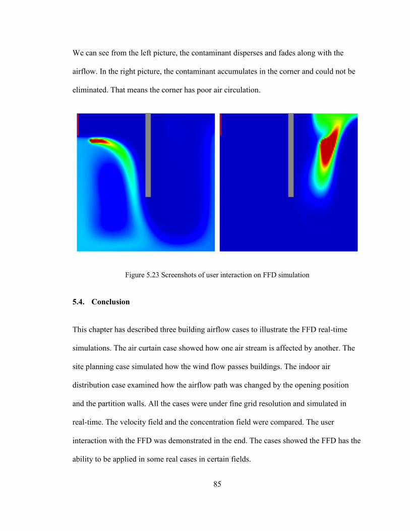
85
We can see from the left picture, the contaminant disperses and fades along with the
airflow. In the right picture, the contaminant accumulates in the corner and could not be
eliminated. That means the corner has poor air circulation.
Figure 5.23 Screenshots of user interaction on FFD simulation
5.4. Conclusion
This chapter has described three building airflow cases to illustrate the FFD real-time
simulations. The air curtain case showed how one air stream is affected by another. The
site planning case simulated how the wind flow passes buildings. The indoor air
distribution case examined how the airflow path was changed by the opening position
and the partition walls. All the cases were under fine grid resolution and simulated in
real-time. The velocity field and the concentration field were compared. The user
interaction with the FFD was demonstrated in the end. The cases showed the FFD has the
ability to be applied in some real cases in certain fields.
86
CHAPTER 6. CONCLUSIONS AND FUTURE WORK
6.1. Conclusions
This thesis studied two methods for the fast simulation of building airflow: the fast fluid
dynamics (FFD) algorithm and the use of graphic processing unit (GPU) for scientific
computing in building engineering. Some major conclusions are summarized as the
following.
The study speeds up the CFD module in CONTAM by porting multi-level “for-
loops” on CPU to parallel calculations on GPU. The best GPU speedup of the
CFD module in CONTAM can be 6.1 folds of the total computing time and 22.5
folds for a single function.
The FFD program could model building airflows in real-time with fine grids
resolution up to 256 × 256.
We improved the FFD by fixing some problems. We found that the traditional
FFD algorithm is not divergence free due to two reasons: the mass imbalance
caused by the use of cell-centered velocities during the calculation of the velocity
divergence for the pressure Poisson equation; and the poor performance of the
Gauss-Seidel linear solver. To fix them, we explicitly defined the cell-face
velocities, which are interpolated to obtain the velocity divergence, and used the
calculated pressures by the pressure Poisson equation to correct the cell-face
velocities directly. We also replaced the Gauss-Seidel solver by a 2-D full
multigrid method, which is able to handle Neumann and inhomogeneous
boundary conditions.
87
A SketchUp model-creating plug-in for the FFD program was also introduced. It
could easily build up the grids, blocks and vents for the FFD models, to enhance
the accessibility of the operation and to extend the range of users.
Three building airflow applications are designed to illustrate the functions and
abilities of the FFD plug-in program. It could simulate the velocity field of
building airflow and the air-borne contaminant transportation in real-time.
The experience and techniques gained from this research will advance building
airflow and contaminant transport modeling on desktop computers, leading to the
ability to model airflows and contaminant transport in real-time or faster.
6.2. Future Work
The current FFD program is still an on-going work due to many limitations. In the future,
the FFD could be improved in many aspects.
The thesis has proved that the current FFD program could simulate the airflow in
real-time with fine grid resolution. The accuracy of the FFD could be improved
and verified.
The current FFD focuses on the simulation speed and visual effects. The
buoyancy and gravity are not well considered in the algorithm.
The FFD plug-in has limited function of generating output data. With the
improvement in codes, more functions of FFD could be developed in the future.
For example, the simulation of airflow driven by temperature difference and the
function of Predicted Mean Vote (PMV) index for indicating indoor comfort
could be added.
88
The speed of FFD could be further accelerated. The study has shown that the
GPU version of CONTAM is faster than the CPU version. If the GPU computing
is combined with FFD in the future, the FFD could be run in real-time with higher
grid resolution. The three-dimensional simulation that usually has more grids
than two-dimensional simulation will become feasible.
The application cases in this thesis are limited to basic and simple problems. More
complex applications can be simulated with corresponding validations in the
future work. A more accurate, more functional and faster FFD will have a broader
application fields in the future.
89
Reference
[1] World Health Organization. "Indoor air pollutants: exposure and health effects," EURO reports and
studies, vol. 78, pp. 1-42, 1983.
[2] D. Menzies and J. Bourbeau, "Building-related illnesses," New England Journal of Medicine, vol. 337,
pp. 1524-1531, 1997.
[3] What is Legionnaires' disease? [Online]. Available:
http://www.osha.gov/dts/osta/otm/legionnaires/disease_rec.html [Accessed: 1 Sep. 2013].
[4] List of Legionellosis outbreaks. [Online]. Available:
http://en.wikipedia.org/wiki/List_of_Legionellosis_outbreaks [Accessed: 1 Sep. 2013].
[5] ASHRAE, "Standard 62.1-2010. Ventilation for Acceptable Indoor Air Quality," ed. Atlanta, GA:
American Society of Heating, Refrigerating and Air-Conditioning Engineers, Inc., 2010.
[6] A.M. Kodama and R. I. McGee, “Airborne Microbial Contaminants in Indoor Environments, Naturally
Ventilated and Air-Conditioned Homes,” Archives of Environmental Health: An International Journal
vol.41, pp. 306-311, 1986.
[7] M. Liddament and M. Orme, "Energy and ventilation," Applied Thermal Engineering, vol. 18, pp.
1101-1109, 1998.[8] ANSYS Fluent [Online]. Available:
http://www.ansys.com/Products/Simulation+Technology/Fluid+Dynamics/Fluid+Dynamics+Products
/ANSYS+Fluent [Accessed: 1 Sep. 2013].
[9] ANSYS CFX [Online]. Available:
http://www.ansys.com/Products/Simulation+Technology/Fluid+Dynamics/Fluid+Dynamics+Products
/ANSYS+CFX [Accessed: 1 Sep. 2013].
[10] PHOENICS [Online]. Available: http://www.cham.co.uk/ [Accessed: 1 Sep. 2013].
[11] Wind Perfect [Online]. Available: http://www.env-simulation.com/ch/sn_sof/index.html [Accessed: 1
Sep. 2013].
[12] CONTAM [Online]. Available: http://www.bfrl.nist.gov/IAQanalysis/CONTAM/overview/2.htm
[Accessed: 1 Sep. 2013].
[13] Z. J. Zhai and Q. Y. Chen, "Performance of coupled building energy and CFD simulations," Energy
and buildings, vol. 37, pp. 333-344, 2005.
[14] J. Axley, "Multizone airflow modeling in buildings: History and theory," HVAC&R Research, vol. 13,
pp. 907-928, 2007.
[15] A. C. Megri and F. Haghighat, "Zonal modeling for simulating indoor environment of buildings:
Review, recent developments, and applications," Hvac&R Research, vol. 13, pp. 887-905, 2007.
[16] L. L. Wang and Q. Chen, "Evaluation of some assumptions used in multizone airflow network
models," Building and Environment, vol. 43, pp. 1671-1677, 2008.
90
[17] A. Schaelin, et al., “Improvement of Multizone Model Predictions by Detailed Flow Path Values from
CFD Calculations.” ASHRAE Transactions, vol. 100(2): pp 709-720, 1994.
[18] H. Moravec, "When will computer hardware match the human brain," Journal of evolution and
technology, vol. 1, p. 10, 1998.
[19] Intel P4004 [Online]. Available: http://www.cpushack.net/chippics/Intel/MCS4/IntelP4004.html
[Accessed: 1 Sep. 2013].
[20] Chip - Intel 80286 Microprocessor Chip [Online]. Available:
http://www.computermuseum.li/Testpage/Chip-Intel80286.htm [Accessed: 1 Sep. 2013].
[21] Sandra - CPU Dhrystone (2004 Oct. 9) [Online]. Available:
http://www.tomshardware.com/charts/cpu-charts-2004/Sandra-CPU-Dhrystone,449.html [Accessed: 1
Sep. 2013].
[22] Synthetic SiSoft Sandra XI CPU (2007) [Online]. Available:
http://www.tomshardware.com/charts/cpu-charts-2007/Synthetic-SiSoft-Sandra-XI-CPU,333.html
[Accessed: 1 Sep. 2013].
[23] ALU Performance: SiSoftware Sandra 2010 Pro (ALU) (2010) [Online]. Available:
http://www.tomshardware.com/charts/desktop-cpu-charts-2010/ALU-Performance-SiSoftware-
Sandra-2010-Pro-ALU,2408.html [Accessed: 1 Sep. 2013].
[24] Kyle Bennett (2011 Nov. 14) Intel Core i7-3960X - Sandy Bridge E Processor Review [Online].
Available: http://hardocp.com/article/2011/11/14/intel_core_i73960x_sandy_bridge_e_processor_
review/4 [Accessed: 1 Sep. 2013].
[25] What is GPU computing? [Online]. Available: http://www.nvidia.com/object/what-is-gpu-
computing.html [Accessed: 1 Sep. 2013].
[26] The World's First GPU [Online]. Available: http://www.nvidia.com/page/geforce256.html [Accessed:
1 Sep. 2013].
[27] GeForce GTX 690 Specifications [Online]. Available: http://www.geforce.com/hardware/desktop-
gpus/geforce-gtx-690/specifications [Accessed: 1 Sep. 2013].
[28] GeForce 600 Series (2013 Jul. 29) [Online]. Available:
http://en.wikipedia.org/wiki/GeForce_600_Series [Accessed: 1 Sep. 2013].
[29] POWER7 [Online]. Available: http://en.wikipedia.org/wiki/POWER7 [Accessed: 1 Sep. 2013].
[30] CUDA C Programming Guide (2013 Jul. 19) [Online]. Available: http://docs.nvidia.com/cuda/cuda-c-
programming-guide/index.html [Accessed: 1 Sep. 2013].
[31] M. Weigel, "Performance potential for simulating spin models on GPU," Journal of Computational
Physics, vol. 231, pp. 3064-3082, 2012.
[32] Y. Zhao, et al. "Efficient decoding of QC-LDPC codes using GPUs," in Algorithms and Architectures
for Parallel Processing, ed: Springer, 2011, pp. 294-305.
[33] J. A. van Meel, et al. "Harvesting graphics power for MD simulations," Molecular Simulation, vol. 34,
pp. 259-266, 2008.
91
[34] J. Stam, "Stable fluids," in Proceedings of the 26th annual conference on Computer graphics and
interactive techniques, 1999, pp. 121-128. [35] M. J. Harris, W. V. Baxter, T. Scheuermann, and A.
Lastra, "Simulation of cloud dynamics on graphics hardware," in Proceedings of the ACM
SIGGRAPH/EUROGRAPHICS conference on Graphics hardware, 2003, pp. 92-101.
[36] N. Rasmussen, et al. "Smoke simulation for large scale phenomena," in ACM Transactions on
Graphics (TOG), 2003, pp. 703-707.
[37] N. S.-H. Chu and C.-L. Tai, "MoXi: real-time ink dispersion in absorbent paper," in ACM
Transactions on Graphics (TOG), 2005, pp. 504-511.
[38] W. Zuo and Q. Chen, "Validation of fast fluid dynamics for room airflow," IBPSA Building Simulation,
2007.
[39] Vertical Industry Solutions [Online]. Available:
http://www.nvidia.com/object/computational_fluid_dynamics.html [Accessed: 1 Sep. 2013].
[40] Lattice Boltzmann methods (2013 Jul. 11) [Online]. Available:
http://en.wikipedia.org/wiki/Lattice_Boltzmann_methods [Accessed: 1 Sep. 2013].
[41] Sailfish Reference Manual (2013 Mar. 14) [Online]. Available: http://sailfish.us.edu.pl/ [Accessed: 1
Sep. 2013].
[42] What is SpeedIT [Online]. Available: http://speedit.vratis.com [Accessed: 1 Sep. 2013].
[43] I. Senocak, et al. "Rapid-response urban CFD simulations using a GPU computing paradigm on
desktop supercomputers," Eighth Symposium on the Urban Environment, 2009.
[44] F. Molnar Jr, et al., "Air pollution modelling using a graphics processing unit with CUDA," Computer
Physics Communications, vol. 181, pp. 105-112, 2010.
[45] W. Zuo and Q. Chen, "Simulations of Air Distributions in Buildings by FFD on GPU," HVAC&R
Research, vol. 16, pp. 785-798, 2010.
[46] Y. Wang, et al., "Implementing CFD (Computational Fluid Dynamics) in OpenCL for Building
Simulation," Proceedings of the 12th international building performance simulation (building
simulation 2011). Sydney, Australia, pp. 1430-1437, 2011.
[47] OpenCL [Online]. Available: http://en.wikipedia.org/wiki/ OpenCL [Accessed: 1 Sep. 2013].
[48] J. Stam, "Interacting with smoke and fire in real time," Communications of the ACM, vol. 43, pp. 76-
83, 2000.
[49] J. Starn, "A simple fluid solver based on the FFT," Journal of graphics tools, vol. 6, pp. 43-52, 2001.
[50] W. Zuo and Q. Chen, "Real‐time or faster‐than‐real‐time simulation of airflow in
buildings," Indoor Air, vol. 19, pp. 33-44, 2009.
[51] A. d. Restivo, "Turbulent flow in ventilated rooms," Imperial College London (University of London),
1979.
[52] W. Zuo, et al., "Improvements in ffd modeling by using different numerical schemes," Numerical Heat
Transfer, Part B: Fundamentals, vol. 58, pp. 1-16, 2010.
92
[53] W. Zuo and Q. Chen, "Fast and informative flow simulations in a building by using fast fluid
dynamics model on graphics processing unit," Building and Environment, vol. 45, pp. 747-757, 2010.
[54] W. Zuo and Q. Chen, "HIGH-PERFORMACNE AND LOW-COST COMPUTING FOR INDOOR
AIRFLOW," in Proc. of Eleventh International IBPSA Conference, 2009, pp. 244-249.
[55] A. Robert, "A stable numerical integration scheme for the primitive meteorological equations,"
Atmosphere-Ocean, vol. 19, pp. 35-46, 1981.
[56] Q. Chen and W. Xu, "A zero-equation turbulence model for indoor airflow simulation," Energy and
buildings, vol. 28, pp. 137-144, 1998.
[57] . H. Ferziger and M. Perić, Computational methods for fluid dynamics, 3 ed. Berlin: Springer, 2002.
[58] A. J. Chorin, "A numerical method for solving incompressible viscous flow problems," Journal of
computational physics, vol. 2, pp. 12-26, 1967.
[59] S. V. Patankar, Numerical heat transfer and fluid flow, New York: McGraw-Hill Book Company,
1980.
[60] J. M. McDonough, Lectures in Computational Fluid Dynamics of Incompressible Flow: Mathematics,
Algorithms and Implementations. Lexington, Department of Mechanical Engineering and
Mathematics, University of Kentucky, 2007
[61] B. P. Leonard, "A stable and accurate convective modelling procedure based on quadratic upstream
interpolation," Computer methods in applied mechanics and engineering, vol. 19, pp. 59-98, 1979.
[62] C. Rhie and W. Chow, "Numerical study of the turbulent flow past an airfoil with trailing edge
separation," AIAA journal, vol. 21, pp. 1525-1532, 1983.
[63] W. H. Press, et al., Numerical Recipes 3rd Edition: The Art of Scientific Computing. New York:
Cambridge University Press, 2007.
[64] W. S. Dols and L. L. Wang. CONTAM 3.0 Tutorial. Gaithersburg: National Institute of Standards and
Technology, 2010.
[65] L. L. Wang, et al., "Using CFD capabilities of CONTAM 3.0 for simulating airflow and contaminant
transport in and around buildings," HVAC&R Research, vol. 16, pp. 749-763, 2010.
[66] About SketchUp [Online]. Available: http://www.sketchup.com/about/sketchup-story [Accessed: 1 Sep.
2013].
[67] Earth As Art [Online]. Available: http://www.nasa.gov/connect/ebooks/earth_art_detail.html
[Accessed: 1 Sep. 2013].
[68] M. Potter and D. C. Wiggert, Schaum's Outline of Fluid Mechanics. New York: McGraw-Hill, 2007.
[69] Masami Sato and T. Kobayashi, "A fundamental study of the flow past a circular cylinder using
Abaqus/CFD," presented at the SIMULIA Community Conference, Providence RI, 2012.
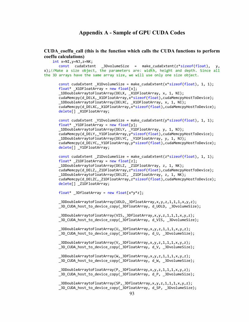
93
Appendix A - Sample of GPU CUDA Codes
CUDA_coeffu_call (this is the function which calls the CUDA functions to perform
coeffu calculations) int x=NI,y=NJ,z=NK;
const cudaExtent _3DvolumeSize = make_cudaExtent(z*sizeof(float), y, x);//Make a size object, the parameters are: width, height and depth. Since all the 3D arrays have the same array size, we will use only one size object. const cudaExtent _X1DvolumeSize = make_cudaExtent(x*sizeof(float), 1, 1); float* _X1DFloatArray = new float[x]; _1DDoubleArraytoFloatArray(DELX, _X1DFloatArray, x, 1, NI); cudaMemcpy(d_DELX,_X1DFloatArray,x*sizeof(float),cudaMemcpyHostToDevice); _1DDoubleArraytoFloatArray(DELXC, _X1DFloatArray, x, 1, NI); cudaMemcpy(d_DELXC,_X1DFloatArray,x*sizeof(float),cudaMemcpyHostToDevice); delete[] _X1DFloatArray; const cudaExtent _Y1DvolumeSize = make_cudaExtent(y*sizeof(float), 1, 1); float* _Y1DFloatArray = new float[y]; _1DDoubleArraytoFloatArray(DELY, _Y1DFloatArray, y, 1, NJ); cudaMemcpy(d_DELY,_Y1DFloatArray,y*sizeof(float),cudaMemcpyHostToDevice); _1DDoubleArraytoFloatArray(DELYC, _Y1DFloatArray, y, 1, NJ); cudaMemcpy(d_DELYC,_Y1DFloatArray,y*sizeof(float),cudaMemcpyHostToDevice); delete[] _Y1DFloatArray; const cudaExtent _Z1DvolumeSize = make_cudaExtent(z*sizeof(float), 1, 1); float* _Z1DFloatArray = new float[z]; _1DDoubleArraytoFloatArray(DELZ, _Z1DFloatArray, z, 1, NK); cudaMemcpy(d_DELZ,_Z1DFloatArray,z*sizeof(float),cudaMemcpyHostToDevice); _1DDoubleArraytoFloatArray(DELZC, _Z1DFloatArray, z, 1, NK); cudaMemcpy(d_DELZC,_Z1DFloatArray,z*sizeof(float),cudaMemcpyHostToDevice); delete[] _Z1DFloatArray; float* _3DfloatArray = new float[x*y*z]; _3DDoubleArraytoFloatArray(UOLD,_3DfloatArray,x,y,z,1,1,1,x,y,z); _3D_CUDA_host_to_device_copy(_3DfloatArray, d_UOLD, _3DvolumeSize); _3DDoubleArraytoFloatArray(VIS,_3DfloatArray,x,y,z,1,1,1,x,y,z); _3D_CUDA_host_to_device_copy(_3DfloatArray, d_VIS, _3DvolumeSize); _3DDoubleArraytoFloatArray(U,_3DfloatArray,x,y,z,1,1,1,x,y,z); _3D_CUDA_host_to_device_copy(_3DfloatArray, d_U, _3DvolumeSize); _3DDoubleArraytoFloatArray(V,_3DfloatArray,x,y,z,1,1,1,x,y,z); _3D_CUDA_host_to_device_copy(_3DfloatArray, d_V, _3DvolumeSize); _3DDoubleArraytoFloatArray(W,_3DfloatArray,x,y,z,1,1,1,x,y,z); _3D_CUDA_host_to_device_copy(_3DfloatArray, d_W, _3DvolumeSize); _3DDoubleArraytoFloatArray(P,_3DfloatArray,x,y,z,1,1,1,x,y,z); _3D_CUDA_host_to_device_copy(_3DfloatArray, d_P, _3DvolumeSize); _3DDoubleArraytoFloatArray(SP,_3DfloatArray,x,y,z,1,1,1,x,y,z); _3D_CUDA_host_to_device_copy(_3DfloatArray, d_SP, _3DvolumeSize);
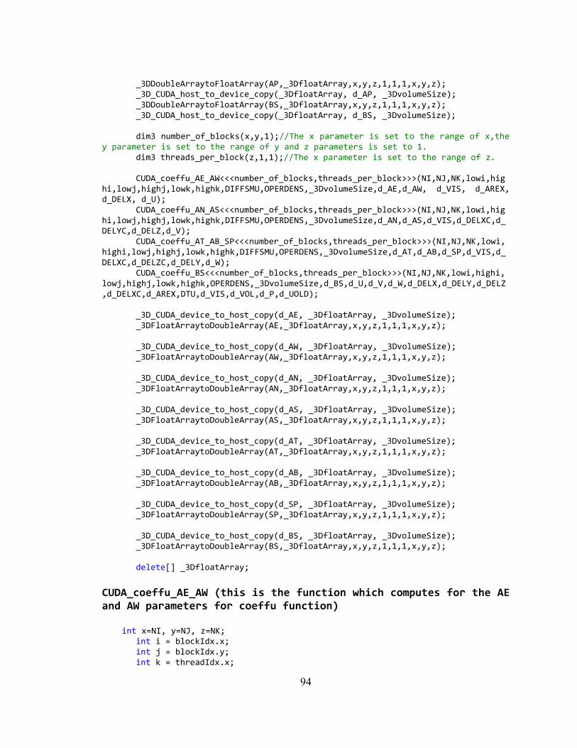
94
_3DDoubleArraytoFloatArray(AP,_3DfloatArray,x,y,z,1,1,1,x,y,z); _3D_CUDA_host_to_device_copy(_3DfloatArray, d_AP, _3DvolumeSize); _3DDoubleArraytoFloatArray(BS,_3DfloatArray,x,y,z,1,1,1,x,y,z); _3D_CUDA_host_to_device_copy(_3DfloatArray, d_BS, _3DvolumeSize); dim3 number_of_blocks(x,y,1);//The x parameter is set to the range of x,the y parameter is set to the range of y and z parameters is set to 1. dim3 threads_per_block(z,1,1);//The x parameter is set to the range of z. CUDA_coeffu_AE_AW<<<number_of_blocks,threads_per_block>>>(NI,NJ,NK,lowi,highi,lowj,highj,lowk,highk,DIFFSMU,OPERDENS,_3DvolumeSize,d_AE,d_AW, d_VIS, d_AREX, d_DELX, d_U); CUDA_coeffu_AN_AS<<<number_of_blocks,threads_per_block>>>(NI,NJ,NK,lowi,highi,lowj,highj,lowk,highk,DIFFSMU,OPERDENS,_3DvolumeSize,d_AN,d_AS,d_VIS,d_DELXC,d_DELYC,d_DELZ,d_V); CUDA_coeffu_AT_AB_SP<<<number_of_blocks,threads_per_block>>>(NI,NJ,NK,lowi,highi,lowj,highj,lowk,highk,DIFFSMU,OPERDENS,_3DvolumeSize,d_AT,d_AB,d_SP,d_VIS,d_DELXC,d_DELZC,d_DELY,d_W); CUDA_coeffu_BS<<<number_of_blocks,threads_per_block>>>(NI,NJ,NK,lowi,highi,lowj,highj,lowk,highk,OPERDENS,_3DvolumeSize,d_BS,d_U,d_V,d_W,d_DELX,d_DELY,d_DELZ,d_DELXC,d_AREX,DTU,d_VIS,d_VOL,d_P,d_UOLD); _3D_CUDA_device_to_host_copy(d_AE, _3DfloatArray, _3DvolumeSize); _3DFloatArraytoDoubleArray(AE,_3DfloatArray,x,y,z,1,1,1,x,y,z); _3D_CUDA_device_to_host_copy(d_AW, _3DfloatArray, _3DvolumeSize); _3DFloatArraytoDoubleArray(AW,_3DfloatArray,x,y,z,1,1,1,x,y,z); _3D_CUDA_device_to_host_copy(d_AN, _3DfloatArray, _3DvolumeSize); _3DFloatArraytoDoubleArray(AN,_3DfloatArray,x,y,z,1,1,1,x,y,z); _3D_CUDA_device_to_host_copy(d_AS, _3DfloatArray, _3DvolumeSize); _3DFloatArraytoDoubleArray(AS,_3DfloatArray,x,y,z,1,1,1,x,y,z); _3D_CUDA_device_to_host_copy(d_AT, _3DfloatArray, _3DvolumeSize); _3DFloatArraytoDoubleArray(AT,_3DfloatArray,x,y,z,1,1,1,x,y,z); _3D_CUDA_device_to_host_copy(d_AB, _3DfloatArray, _3DvolumeSize); _3DFloatArraytoDoubleArray(AB,_3DfloatArray,x,y,z,1,1,1,x,y,z); _3D_CUDA_device_to_host_copy(d_SP, _3DfloatArray, _3DvolumeSize); _3DFloatArraytoDoubleArray(SP,_3DfloatArray,x,y,z,1,1,1,x,y,z); _3D_CUDA_device_to_host_copy(d_BS, _3DfloatArray, _3DvolumeSize); _3DFloatArraytoDoubleArray(BS,_3DfloatArray,x,y,z,1,1,1,x,y,z); delete[] _3DfloatArray;
CUDA_coeffu_AE_AW (this is the function which computes for the AE and AW parameters for coeffu function)
int x=NI, y=NJ, z=NK; int i = blockIdx.x; int j = blockIdx.y; int k = threadIdx.x;
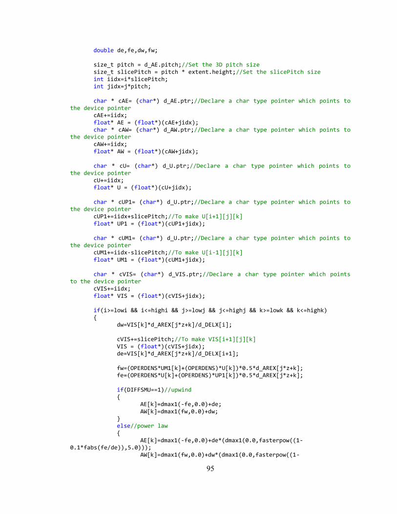
95
double de,fe,dw,fw; size_t pitch = d_AE.pitch;//Set the 3D pitch size size_t slicePitch = pitch * extent.height;//Set the slicePitch size int iidx=i*slicePitch; int jidx=j*pitch; char * cAE= (char*) d_AE.ptr;//Declare a char type pointer which points to the device pointer cAE+=iidx; float* AE = (float*)(cAE+jidx); char * cAW= (char*) d_AW.ptr;//Declare a char type pointer which points to the device pointer cAW+=iidx; float* AW = (float*)(cAW+jidx); char * cU= (char*) d_U.ptr;//Declare a char type pointer which points to the device pointer cU+=iidx; float* U = (float*)(cU+jidx); char * cUP1= (char*) d_U.ptr;//Declare a char type pointer which points to the device pointer cUP1+=iidx+slicePitch;//To make U[i+1][j][k] float* UP1 = (float*)(cUP1+jidx); char * cUM1= (char*) d_U.ptr;//Declare a char type pointer which points to the device pointer cUM1+=iidx-slicePitch;//To make U[i-1][j][k] float* UM1 = (float*)(cUM1+jidx); char * cVIS= (char*) d_VIS.ptr;//Declare a char type pointer which points to the device pointer cVIS+=iidx; float* VIS = (float*)(cVIS+jidx); if(i>=lowi && i<=highi && j>=lowj && j<=highj && k>=lowk && k<=highk) { dw=VIS[k]*d_AREX[j*z+k]/d_DELX[i]; cVIS+=slicePitch;//To make VIS[i+1][j][k] VIS = (float*)(cVIS+jidx); de=VIS[k]*d_AREX[j*z+k]/d_DELX[i+1]; fw=(OPERDENS*UM1[k]+(OPERDENS)*U[k])*0.5*d_AREX[j*z+k]; fe=(OPERDENS*U[k]+(OPERDENS)*UP1[k])*0.5*d_AREX[j*z+k]; if(DIFFSMU==1)//upwind { AE[k]=dmax1(-fe,0.0)+de; AW[k]=dmax1(fw,0.0)+dw; } else//power law { AE[k]=dmax1(-fe,0.0)+de*(dmax1(0.0,fasterpow((1-0.1*fabs(fe/de)),5.0))); AW[k]=dmax1(fw,0.0)+dw*(dmax1(0.0,fasterpow((1-
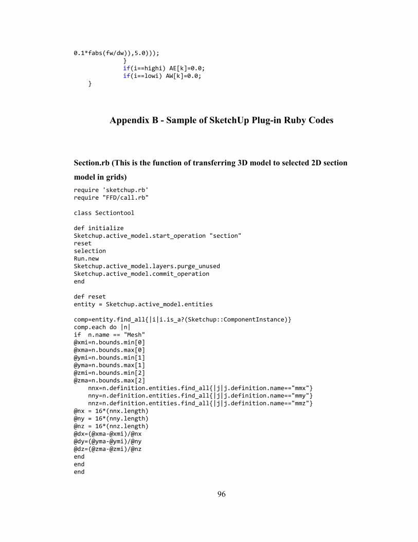
96
0.1*fabs(fw/dw)),5.0))); } if(i==highi) AE[k]=0.0; if(i==lowi) AW[k]=0.0; }
Appendix B - Sample of SketchUp Plug-in Ruby Codes
Section.rb (This is the function of transferring 3D model to selected 2D section
model in grids)
require 'sketchup.rb' require "FFD/call.rb" class Sectiontool def initialize Sketchup.active_model.start_operation "section" reset selection Run.new Sketchup.active_model.layers.purge_unused Sketchup.active_model.commit_operation end def reset entity = Sketchup.active_model.entities comp=entity.find_all{|i|i.is_a?(Sketchup::ComponentInstance)} comp.each do |n| if n.name == "Mesh" @xmi=n.bounds.min[0] @xma=n.bounds.max[0] @ymi=n.bounds.min[1] @yma=n.bounds.max[1] @zmi=n.bounds.min[2] @zma=n.bounds.max[2] nnx=n.definition.entities.find_all{|j|j.definition.name=="mmx"} nny=n.definition.entities.find_all{|j|j.definition.name=="mmy"} nnz=n.definition.entities.find_all{|j|j.definition.name=="mmz"} @nx = 16*(nnx.length) @ny = 16*(nny.length) @nz = 16*(nnz.length) @dx=(@xma-@xmi)/@nx @dy=(@yma-@ymi)/@ny @dz=(@zma-@zmi)/@nz end end end
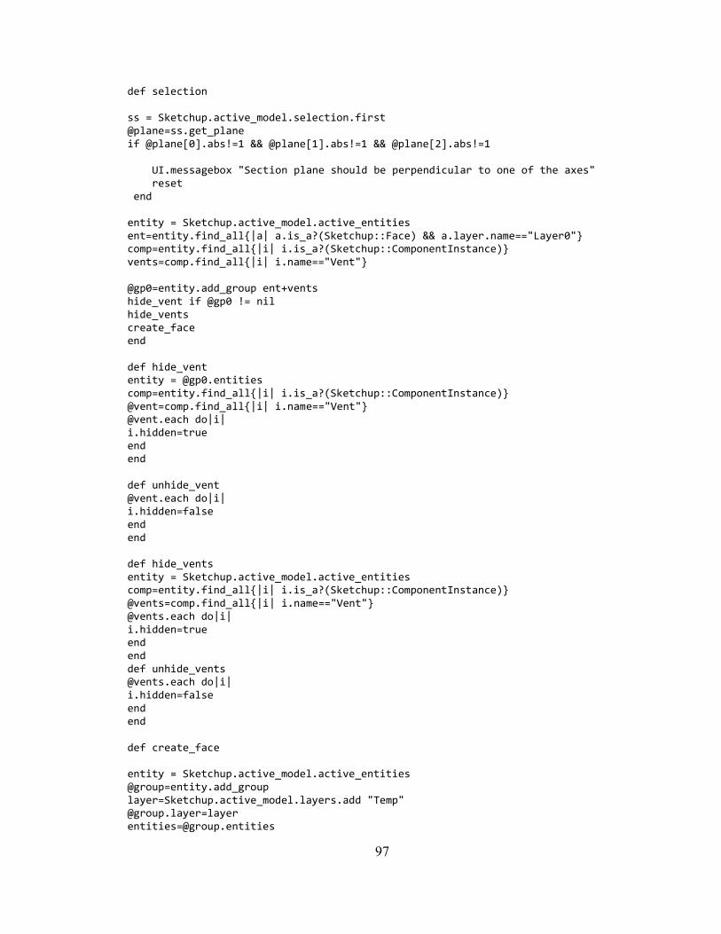
97
def selection ss = Sketchup.active_model.selection.first @plane=ss.get_plane if @plane[0].abs!=1 && @plane[1].abs!=1 && @plane[2].abs!=1 UI.messagebox "Section plane should be perpendicular to one of the axes" reset end entity = Sketchup.active_model.active_entities ent=entity.find_all{|a| a.is_a?(Sketchup::Face) && a.layer.name=="Layer0"} comp=entity.find_all{|i| i.is_a?(Sketchup::ComponentInstance)} vents=comp.find_all{|i| i.name=="Vent"} @gp0=entity.add_group ent+vents hide_vent if @gp0 != nil hide_vents create_face end def hide_vent entity = @gp0.entities comp=entity.find_all{|i| i.is_a?(Sketchup::ComponentInstance)} @vent=comp.find_all{|i| i.name=="Vent"} @vent.each do|i| i.hidden=true end end def unhide_vent @vent.each do|i| i.hidden=false end end def hide_vents entity = Sketchup.active_model.active_entities comp=entity.find_all{|i| i.is_a?(Sketchup::ComponentInstance)} @vents=comp.find_all{|i| i.name=="Vent"} @vents.each do|i| i.hidden=true end end def unhide_vents @vents.each do|i| i.hidden=false end end def create_face entity = Sketchup.active_model.active_entities @group=entity.add_group layer=Sketchup.active_model.layers.add "Temp" @group.layer=layer [email protected]
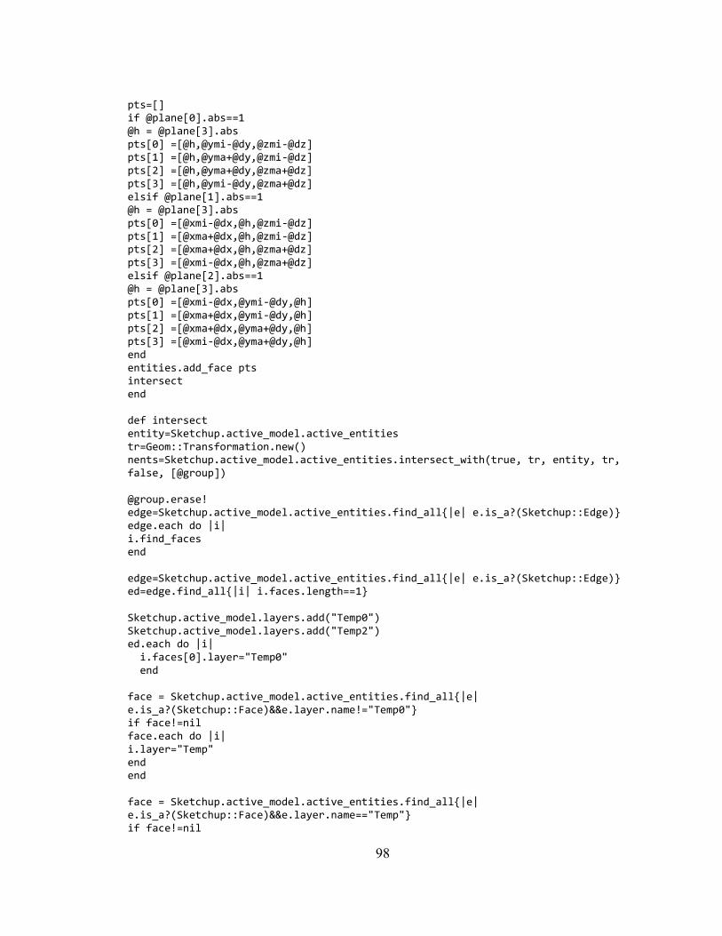
98
pts=[] if @plane[0].abs==1 @h = @plane[3].abs pts[0] =[@h,@ymi-@dy,@zmi-@dz] pts[1] =[@h,@yma+@dy,@zmi-@dz] pts[2] =[@h,@yma+@dy,@zma+@dz] pts[3] =[@h,@ymi-@dy,@zma+@dz] elsif @plane[1].abs==1 @h = @plane[3].abs pts[0] =[@xmi-@dx,@h,@zmi-@dz] pts[1] =[@xma+@dx,@h,@zmi-@dz] pts[2] =[@xma+@dx,@h,@zma+@dz] pts[3] =[@xmi-@dx,@h,@zma+@dz] elsif @plane[2].abs==1 @h = @plane[3].abs pts[0] =[@xmi-@dx,@ymi-@dy,@h] pts[1] =[@xma+@dx,@ymi-@dy,@h] pts[2] =[@xma+@dx,@yma+@dy,@h] pts[3] =[@xmi-@dx,@yma+@dy,@h] end entities.add_face pts intersect end def intersect entity=Sketchup.active_model.active_entities tr=Geom::Transformation.new() nents=Sketchup.active_model.active_entities.intersect_with(true, tr, entity, tr, false, [@group]) @group.erase! edge=Sketchup.active_model.active_entities.find_all{|e| e.is_a?(Sketchup::Edge)} edge.each do |i| i.find_faces end edge=Sketchup.active_model.active_entities.find_all{|e| e.is_a?(Sketchup::Edge)} ed=edge.find_all{|i| i.faces.length==1} Sketchup.active_model.layers.add("Temp0") Sketchup.active_model.layers.add("Temp2") ed.each do |i| i.faces[0].layer="Temp0" end face = Sketchup.active_model.active_entities.find_all{|e| e.is_a?(Sketchup::Face)&&e.layer.name!="Temp0"} if face!=nil face.each do |i| i.layer="Temp" end end face = Sketchup.active_model.active_entities.find_all{|e| e.is_a?(Sketchup::Face)&&e.layer.name=="Temp"} if face!=nil
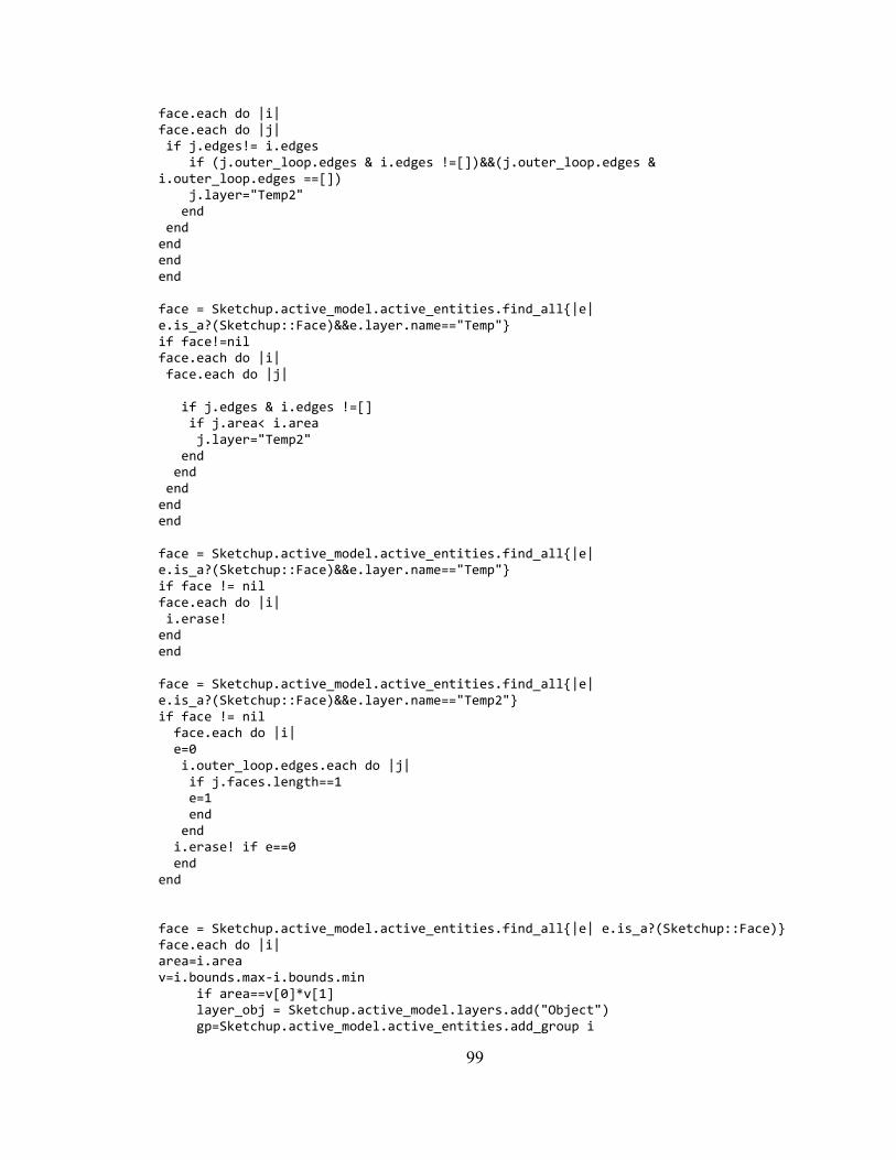
99
face.each do |i| face.each do |j| if j.edges!= i.edges if (j.outer_loop.edges & i.edges !=[])&&(j.outer_loop.edges & i.outer_loop.edges ==[]) j.layer="Temp2" end end end end end face = Sketchup.active_model.active_entities.find_all{|e| e.is_a?(Sketchup::Face)&&e.layer.name=="Temp"} if face!=nil face.each do |i| face.each do |j| if j.edges & i.edges !=[] if j.area< i.area j.layer="Temp2" end end end end end face = Sketchup.active_model.active_entities.find_all{|e| e.is_a?(Sketchup::Face)&&e.layer.name=="Temp"} if face != nil face.each do |i| i.erase! end end face = Sketchup.active_model.active_entities.find_all{|e| e.is_a?(Sketchup::Face)&&e.layer.name=="Temp2"} if face != nil face.each do |i| e=0 i.outer_loop.edges.each do |j| if j.faces.length==1 e=1 end end i.erase! if e==0 end end face = Sketchup.active_model.active_entities.find_all{|e| e.is_a?(Sketchup::Face)} face.each do |i| area=i.area v=i.bounds.max-i.bounds.min if area==v[0]*v[1] layer_obj = Sketchup.active_model.layers.add("Object") gp=Sketchup.active_model.active_entities.add_group i
100
gp.layer = layer_obj gp.entities.each {|e| e.layer=layer_obj} else gp=Sketchup.active_model.active_entities.add_group i gp.layer = "Temp" gp.entities.each {|e| e.layer="Temp"} end end change_face end def change_face entity = Sketchup.active_model.active_entities gt=entity.find_all{|g| (g.is_a?(Sketchup::Group) && g.layer.name == "Temp")} gt.each do |i| sxmin = (((i.bounds.min[0]-@xmi)/@dx).floor)*@dx + @xmi symin = (((i.bounds.min[1]-@ymi)/@dy).floor)*@dy + @ymi szmin = (((i.bounds.min[2]-@zmi)/@dz).floor)*@dz + @zmi nx= ((i.bounds.max[0]-sxmin)/@dx).ceil ny= ((i.bounds.max[1]-symin)/@dy).ceil nz= ((i.bounds.max[2]-szmin)/@dz).ceil ox=i.bounds.min[0] oy=i.bounds.min[1] oz=i.bounds.min[2] group = i.entities.add_group group.layer="Temp" entities=group.entities pts=[] if @plane[0].abs==1 (1..ny).each do |y| pts[0]=[0,(symin-oy+y*@dy-@dy/2),(szmin-oz)] pts[1]=[0,(symin-oy+y*@dy-@dy/2),(szmin-oz+nz*@dz)] entities.add_line pts end elsif @plane[1].abs==1 (1..nx).each do |x| pts[0]=[(sxmin-ox+x*@dx-@dx/2),0,(szmin-oz)] pts[1]=[(sxmin-ox+x*@dx-@dx/2),0,(szmin-oz+nz*@dz)] entities.add_line pts end elsif @plane[2].abs==1 (1..nx).each do |x| pts[0]=[(sxmin-ox+x*@dx-@dx/2),(symin-oy),0] pts[1]=[(sxmin-ox+x*@dx-@dx/2),(symin-oy+ny*@dy),0] entities.add_line pts end end tr=Geom::Transformation.new() nents=i.entities.intersect_with(true, tr, i, tr, false, [group]) group.erase! edge=i.entities.find_all{|e| e.is_a?(Sketchup::Edge) && e.faces.length==1 }
101
if edge !=nil edge.each do |d| d.erase! end end pt=[] if @plane[0].abs==1 edge=i.entities.find_all{|e| e.is_a?(Sketchup::Edge) } edge.each do |e| p1=e.start.position p2=e.end.position pt[0]=[p1.x,(p1.y - @dy/2),((((p1.z+oz-@zmi)/@dz).round)*@dz+@zmi-oz)] pt[1]=[p1.x,(p1.y + @dy/2),((((p1.z+oz-@zmi)/@dz).round)*@dz+@zmi-oz)] pt[2]=[p2.x,(p2.y + @dy/2),((((p2.z+oz-@zmi)/@dz).round)*@dz+@zmi-oz)] pt[3]=[p2.x,(p2.y - @dy/2),((((p2.z+oz-@zmi)/@dz).round)*@dz+@zmi-oz)] if pt[0]!=pt[3] fc=i.entities.add_face pt fc.layer="Temp" end e.erase! end edge=i.entities.find_all{|e| e.is_a?(Sketchup::Edge) && e.faces.length==2 } edge.each do |e| if e.faces[0].bounds.max[2]==e.faces[1].bounds.max[2] && e.faces[0].bounds.min[2]==e.faces[1].bounds.min[2] e.erase! end end elsif @plane[1].abs==1 edge=i.entities.find_all{|e| e.is_a?(Sketchup::Edge) } edge.each do |e| p1=e.start.position p2=e.end.position pt[0]=[(p1.x - @dx/2),p1.y,((((p1.z+oz-@zmi)/@dz).round)*@dz+@zmi-oz)] pt[1]=[(p1.x + @dx/2),p2.y,((((p1.z+oz-@zmi)/@dz).round)*@dz+@zmi-oz)] pt[2]=[(p2.x + @dx/2),p2.y,((((p2.z+oz-@zmi)/@dz).round)*@dz+@zmi-oz)] pt[3]=[(p2.x - @dx/2),p2.y,((((p2.z+oz-@zmi)/@dz).round)*@dz+@zmi-oz)] if pt[0]!=pt[3] fc=i.entities.add_face pt fc.layer="Temp" end e.erase! end edge=i.entities.find_all{|e| e.is_a?(Sketchup::Edge) && e.faces.length==2 } edge.each do |e| if e.faces[0].bounds.max[2]==e.faces[1].bounds.max[2] && e.faces[0].bounds.min[2]==e.faces[1].bounds.min[2] e.erase! end end elsif @plane[2].abs==1 edge=i.entities.find_all{|e| e.is_a?(Sketchup::Edge) } edge.each do |e| p1=e.start.position p2=e.end.position pt[0]=[(p1.x - @dx/2),((((p1.y+oy-@ymi)/@dy).round)*@dy+@ymi-oy),p1.z]
102
pt[1]=[(p1.x + @dx/2),((((p1.y+oy-@ymi)/@dy).round)*@dy+@ymi-oy),p1.z] pt[2]=[(p2.x + @dx/2),((((p2.y+oy-@ymi)/@dy).round)*@dy+@ymi-oy),p2.z] pt[3]=[(p2.x - @dx/2),((((p2.y+oy-@ymi)/@dy).round)*@dy+@ymi-oy),p2.z] if pt[0]!=pt[3] fc=i.entities.add_face pt fc.layer="Temp" end e.erase! end edge=i.entities.find_all{|e| e.is_a?(Sketchup::Edge) && e.faces.length==2 } edge.each do |e| if e.faces[0].bounds.max[1]==e.faces[1].bounds.max[1] && e.faces[0].bounds.min[1]==e.faces[1].bounds.min[1] e.erase! end end end end change_2 end def change_2 entity=Sketchup.active_model.active_entities gt=entity.find_all{|g| (g.is_a?(Sketchup::Group) && g.layer.name == "Temp")} gt.each do |i| i.explode end face=entity.find_all{|f| f.is_a?(Sketchup::Face) } layer=Sketchup.active_model.layers.add("Object") face.each do |j| gp=entity.add_group j gp.layer=layer gp.entities.each {|k| k.layer = layer} end edge=entity.find_all{|f| f.is_a?(Sketchup::Edge) } if edge!=nil edge.each do |e| e.erase! end end unhide_vent if @gp0 != nil @gp0.explode if @gp0 != nil unhide_vents end end #====================================================================== UI.add_context_menu_handler do |menu| ss = Sketchup.active_model.selection.first if ss.typename == "SectionPlane" menu.add_separator menu.add_item("Run simulation") {Sectiontool.new} end
end
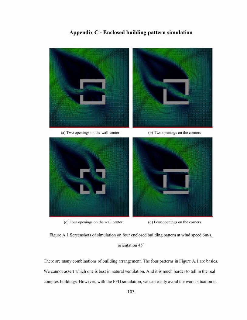
103
Appendix C - Enclosed building pattern simulation
(a) Two openings on the wall center (b) Two openings on the corners
(c) Four openings on the wall center (d) Four openings on the corners
Figure A.1 Screenshots of simulation on four enclosed building pattern at wind speed 6m/s,
orientation 45º
There are many combinations of building arrangement. The four patterns in Figure A.1 are basics.
We cannot assert which one is best in natural ventilation. And it is much harder to tell in the real
complex buildings. However, with the FFD simulation, we can easily avoid the worst situation in
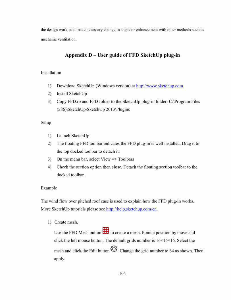
104
the design work, and make necessary change in shape or enhancement with other methods such as
mechanic ventilation.
Appendix D – User guide of FFD SketchUp plug-in
Installation
1) Download SketchUp (Windows version) at http://www.sketchup.com
2) Install SketchUp
3) Copy FFD.rb and FFD folder to the SketchUp plug-in folder: C:\Program Files
(x86)\SketchUp\SketchUp 2013\Plugins
Setup
1) Launch SketchUp
2) The floating FFD toolbar indicates the FFD plug-in is well installed. Drag it to
the top docked toolbar to detach it.
3) On the menu bar, select View => Toolbars
4) Check the section option then close. Detach the floating section toolbar to the
docked toolbar.
Example
The wind flow over pitched roof case is used to explain how the FFD plug-in works.
More SketchUp tutorials please see http://help.sketchup.com/en.
1) Create mesh.
Use the FFD Mesh button to create a mesh. Point a position by move and
click the left mouse button. The default grids number is 16×16×16. Select the
mesh and click the Edit button . Change the grid number to 64 as shown. Then
apply.
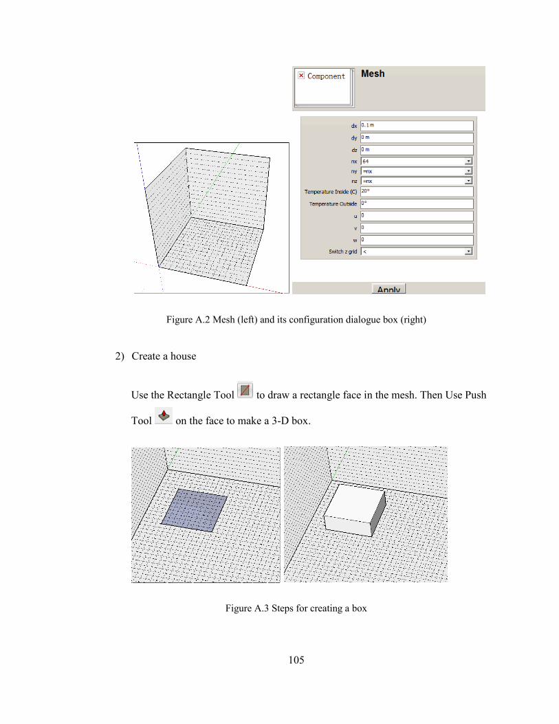
105
Figure A.2 Mesh (left) and its configuration dialogue box (right)
2) Create a house
Use the Rectangle Tool to draw a rectangle face in the mesh. Then Use Push
Tool on the face to make a 3-D box.
Figure A.3 Steps for creating a box
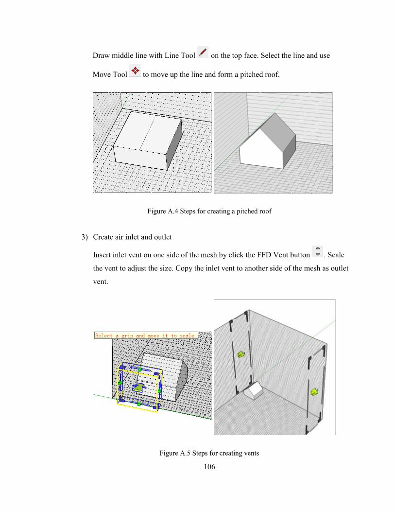
106
Draw middle line with Line Tool on the top face. Select the line and use
Move Tool to move up the line and form a pitched roof.
Figure A.4 Steps for creating a pitched roof
3) Create air inlet and outlet
Insert inlet vent on one side of the mesh by click the FFD Vent button . Scale
the vent to adjust the size. Copy the inlet vent to another side of the mesh as outlet
vent.
Figure A.5 Steps for creating vents
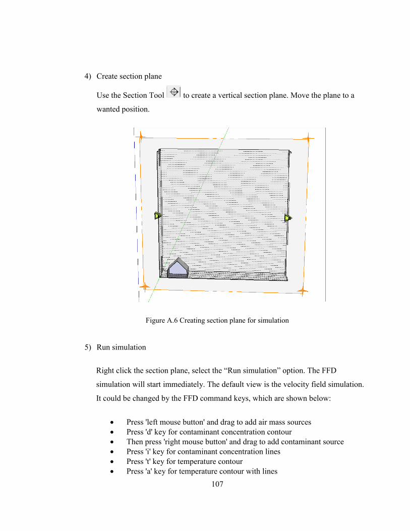
107
4) Create section plane
Use the Section Tool to create a vertical section plane. Move the plane to a
wanted position.
Figure A.6 Creating section plane for simulation
5) Run simulation
Right click the section plane, select the “Run simulation” option. The FFD
simulation will start immediately. The default view is the velocity field simulation.
It could be changed by the FFD command keys, which are shown below:
Press 'left mouse button' and drag to add air mass sources
Press 'd' key for contaminant concentration contour
Then press 'right mouse button' and drag to add contaminant source
Press 'i' key for contaminant concentration lines
Press 't' key for temperature contour
Press 'a' key for temperature contour with lines
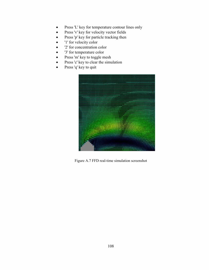
108
Press 'L' key for temperature contour lines only
Press 'v' key for velocity vector fields
Press 'p' key for particle tracking then
'1' for velocity color
'2' for concentration color
'3' for temperature color
Press 'm' key to toggle mesh
Press 'c' key to clear the simulation
Press 'q' key to quit
Figure A.7 FFD real-time simulation screenshot


![GPU based virtual screening techniques for faster drug ...people.cse.nitc.ac.in/jayaraj/files/thesis_ppt1.pdf · Computer aided Drug Discovery[65] GPU based virtual screening techniques](https://img.pdfslide.us/doc/110x75/5ece4d4cb1af104f892b6793/gpu-based-virtual-screening-techniques-for-faster-drug-computer-aided-drug-discovery65.jpg)