Embed Size (px)
Citation preview

IN DEGREE PROJECT COMPUTER SCIENCE AND ENGINEERING,SECOND CYCLE, 30 CREDITS
, STOCKHOLM SWEDEN 2016
Real-time analysis, in SuperCollider, of spectral features of electroglottographic signals
DENNIS JOHANSSON
KTH ROYAL INSTITUTE OF TECHNOLOGYSCHOOL OF COMPUTER SCIENCE AND COMMUNICATION

Real-time analysis, in SuperCollider, of spectral features of
electroglottographic signals
Analys i realtid, i SuperCollider, av spektrala egenskaper
hos elektroglottografiska signaler
Dennis Johansson
DD221X; Degree Project in Computer Science, Second Cycle (30 ECTS credits)
Degree Program in Computer Science and Engineering (300 ECTS credits)
Royal Institute of Technology year 2016
School of Computer Science and Communication (CSC)
Supervisor was Sten Ternström
Examiner was Olov Engwall
Royal Institute of Technology School of Computer Science and Communication
KTH CSC
SE-100 44 Stockholm, Sweden
URL: www.kth.se/csc
Abstract
This thesis presents tools and components necessary to further develop
an implementation of a method. The method attempts to use the non-
invasive electroglottographic signal to locate rapid transitions between
voice registers. Implementations for sample entropy and the Discrete
Fourier Transform (DFT) implemented for the programming language
SuperCollider are presented along with tools necessary to evaluate the
method and present the results in real time.
Since different algorithms have been used, both for clustering and cycle
separation, a comparison between algorithms for both of these steps
has also been done.
Referat
Denna rapport presenterar verktyg och komponenter som är
nödvändiga för att vidareutveckla en implementation av en metod.
Metoden försöker att använda en icke invasiv elektroglottografisk
signal för att hitta snabba övergångar mellan röstregister. Det
presenteras implementationer för sampelentropi och den diskreta
fouriertransformen för programspråket SuperCollider samt verktyg som
behövs för att utvärdera metoden och presentera resultaten i realtid.
Då olika algoritmer har använts för både klustring och cykelseparation
så har även en jämförelse mellan algoritmer för dessa steg gjorts.

I would like to start by thanking my supervisor for this project, Sten
Ternström, for many good discussions about the master thesis and feedback
during the implementation phase.
Thank you Andreas Selamtzis for providing me with the necessary
information from the MATLAB implementation.
Thank you Andreas Wedenborn, Christoffer Carlsson, David Sandberg, Jens
Eriksson and Niklas Bäckström for feedback on this master thesis.
Thank you Olov Engwall for examining this master thesis.
Finally, thank you dad, Jan Johansson, for proofreading this thesis.

Table of Contents 1 Introduction ........................................................................................................................................... 1
1.1 Related Work ................................................................................................................................. 2
1.2 Previous Work ............................................................................................................................... 2
2 Target Algorithm ................................................................................................................................... 4
3 Overview ................................................................................................................................................ 6
4 SuperCollider ......................................................................................................................................... 7
4.1 The Server Side .............................................................................................................................. 7
4.2 The Client Side ............................................................................................................................... 9
5 Data Transfer ....................................................................................................................................... 13
5.1 Server to Client ............................................................................................................................ 13
5.1.1 Problem ............................................................................................................................... 13
5.1.2 Trivial Solution? ................................................................................................................... 13
5.1.3 Streaming Data .................................................................................................................... 14
5.2 Server to File ................................................................................................................................ 17
6 Cycle Separation .................................................................................................................................. 19
6.1 Phase Portrait .............................................................................................................................. 19
6.2 Peak Follower .............................................................................................................................. 19
6.3 Comparative Analysis .................................................................................................................. 21
6.4 Results ......................................................................................................................................... 23
6.5 Analysis ........................................................................................................................................ 24
6.6 Conclusion ................................................................................................................................... 25
7 Discrete Fourier Transform ................................................................................................................. 26
8 Sample Entropy ................................................................................................................................... 28
8.1 Options ........................................................................................................................................ 28
8.1.1 Naïve Algorithm ................................................................................................................... 28
8.1.2 Fast Algorithm ..................................................................................................................... 29
8.2 Optimization ................................................................................................................................ 29
9 Clustering ............................................................................................................................................. 32
9.1 Problem ....................................................................................................................................... 32
9.2 Options ........................................................................................................................................ 33
9.2.1 KMeansRT ............................................................................................................................ 33
9.2.2 K-Means ............................................................................................................................... 34

9.2.3 Gaussian Mixture Model through Expectation Maximization ............................................ 35
9.2.4 Fuzzy C-Means ..................................................................................................................... 36
9.3 Determining the Number of Clusters .......................................................................................... 37
9.4 Comparative Analysis .................................................................................................................. 38
9.4.1 Definition of Good Clustering .............................................................................................. 38
9.4.2 Results & Analysis ................................................................................................................ 40
10 Graphical User Interface .................................................................................................................. 47
10.1 Overview ...................................................................................................................................... 47
10.2 Moving EGG ................................................................................................................................. 48
10.3 Average Cycle per Cluster ............................................................................................................ 49
11 Conclusion & Future Work .............................................................................................................. 51
References ................................................................................................................................................... 53
Appendix A: Rates ....................................................................................................................................... 56
Appendix B: Detailed Process ...................................................................................................................... 63
1
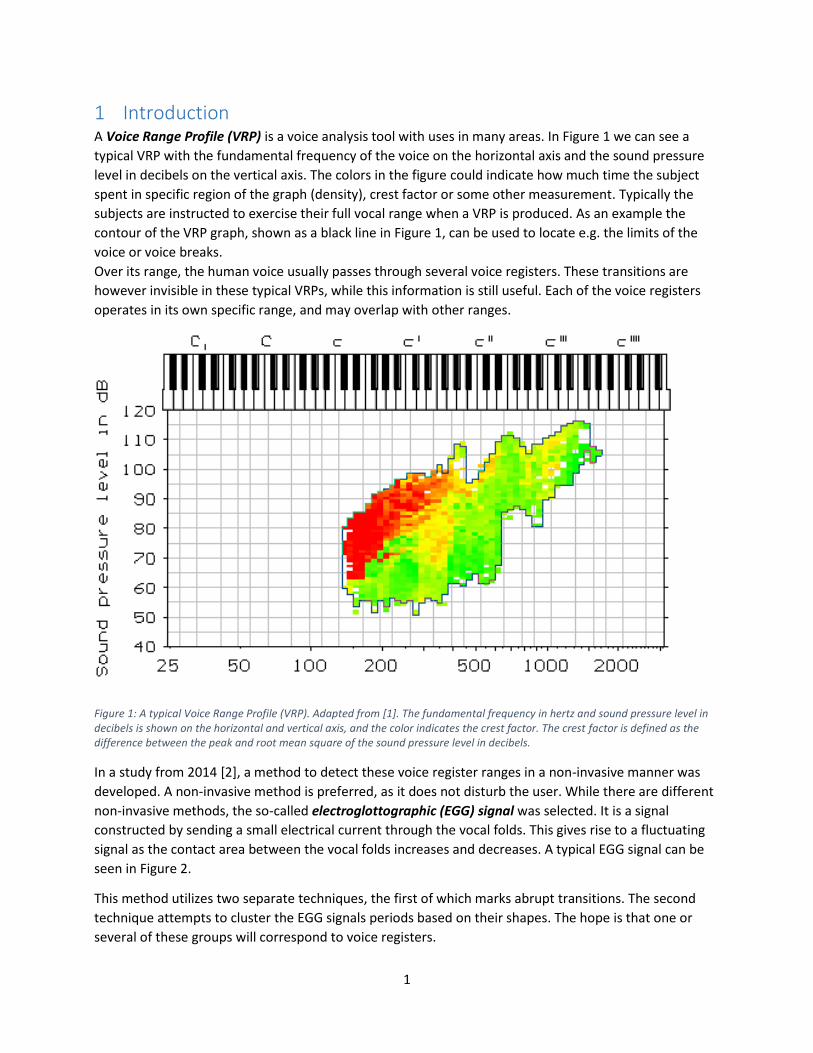
1 Introduction A Voice Range Profile (VRP) is a voice analysis tool with uses in many areas. In Figure 1 we can see a
typical VRP with the fundamental frequency of the voice on the horizontal axis and the sound pressure
level in decibels on the vertical axis. The colors in the figure could indicate how much time the subject
spent in specific region of the graph (density), crest factor or some other measurement. Typically the
subjects are instructed to exercise their full vocal range when a VRP is produced. As an example the
contour of the VRP graph, shown as a black line in Figure 1, can be used to locate e.g. the limits of the
voice or voice breaks.
Over its range, the human voice usually passes through several voice registers. These transitions are
however invisible in these typical VRPs, while this information is still useful. Each of the voice registers
operates in its own specific range, and may overlap with other ranges.
Figure 1: A typical Voice Range Profile (VRP). Adapted from [1]. The fundamental frequency in hertz and sound pressure level in decibels is shown on the horizontal and vertical axis, and the color indicates the crest factor. The crest factor is defined as the difference between the peak and root mean square of the sound pressure level in decibels.
In a study from 2014 [2], a method to detect these voice register ranges in a non-invasive manner was
developed. A non-invasive method is preferred, as it does not disturb the user. While there are different
non-invasive methods, the so-called electroglottographic (EGG) signal was selected. It is a signal
constructed by sending a small electrical current through the vocal folds. This gives rise to a fluctuating
signal as the contact area between the vocal folds increases and decreases. A typical EGG signal can be
seen in Figure 2.
This method utilizes two separate techniques, the first of which marks abrupt transitions. The second
technique attempts to cluster the EGG signals periods based on their shapes. The hope is that one or
several of these groups will correspond to voice registers.

2
Figure 2: A typical EGG signal. Each period in the signal indicates one cycle in the movement of the vocal folds. The horizontal axis is time (about 20 ms), and the vertical axis is contact area (arbitrary scale).
The main goal of the master thesis is to process the incoming signals and present the transitions and
classifications in real time using the programming language SuperCollider, while the user is vocalizing or
a recording is playing. Since this may prove difficult to cluster in real time, an exception has been made.
If it is required for sufficient results, clustering may be applied as a post-processing step.
Once the real time version has been fully implemented, the method can be evaluated by pedagogues
and clinicians. It is also planned for a candidate or master thesis student to perform an evaluation of the
method using the real time implementation. Once this evaluation is done, the method can be further
improved.
This master thesis discusses and implements an initial real time version of the method, to see where its
limits are. Whether this is possible or not, with or without SuperCollider, is the main question that
requires an answer, since this implementation is meant for further research. Thus, any environmental or
sustainability aspects are negligible. One could argue that there is an ethical and social impact, since
negative results may prevent or stall the research, which this project assists.
1.1 Related Work Two common uses for VRPs are to detect vocal pathologies and to enhance voice register management
for singers. For example, in 2004, the VRP of 42 subjects of varying singing technique levels, ranging from
professional singers to subjects without any experience in singing, was used to gain new information for
voice register management in singing practice [3]. The VRP can also be used to detect voice pathologies,
as seen in a study from 1998 [4], where VRPs were used to evaluate vocal performances of children. 94
ordinary children and 136 children with vocal pathologies participated, and by using the VRP data, along
with the age of the subjects, a voice range profile index for children was produced. This was later used to
rate the vocal performance of children, from healthy to dysphonic, with a high sensitivity and specificity.
More examples and an overview of the VRP as a voice analysis tool is given in [5].
The most common use for SC as a programming language is for generating music, as a live performance
or recording. There are hundreds of music projects on GitHub, along with many recordings from alleged
live performances. Among the projects on GitHub, there are also a few master thesis projects [6] [7],
although not any similar to this one. There are also programming courses using SC as a fun interactive
way of teaching programming [8].
1.2 Previous Work This work was originally started by the authors of [2]. The first implementation was done in MATLAB.
Although the initial analysis made in [2] was fairly limited with only two voice registers, modal and
falsetto, with three subjects, it proved successful. With these results, a project was started with the
intent to implement a real time equivalent of the successful MATLAB implementation. Since the
implementation did not entirely rely on knowing the entire recording, this was assumed possible.

3
One of the essential aspects of the VRP is the real-time feedback that it can provide to the voice patient
or voice student. Voice production is a complex process; visual feedback can help to focus the attention
both of the subject and of the clinician or researcher. This is true even when listening to recorded
productions. Since the algorithm incrementally builds the VRP, there exists a connection between the
part of the VRP that is improved at any given time and the algorithm’s input. With a real time algorithm
this feedback is immediate. As an example; a lack of density “above” the region in the VRP that was
touched by an exercise, could indicate that the subject should repeat that exercise, but attempt to
vocalize louder. Although modern MATLAB platforms are reasonably fast, they are limited in their real-
time capabilities.
The authors of [2] started to implement the real time version in a programming language called
SuperCollider [9]. SuperCollider (SC) is a programming language originally developed by James
McCartney, and later made into an open source project [10]. The language is primarily used for real time
audio synthesis and algorithmic composition. Since implementing a real time version of the MATLAB
implementation is time consuming, a bachelor science thesis degree project was formed. The bachelor
science thesis project focused on one of the required components, namely implementing the Fourier
analysis of the EGG signal in real time [11]. Henceforth the real time implementation done before this
degree project started will be referred to as the given prototype.

4
2 Target Algorithm
Figure 3: The overall structure of the algorithm, starting from the left and moving to the right.
This section introduces the algorithm from the study referred to in the introduction [2]. Figure 3 gives an
overview of components of the algorithm, and where these are described in this thesis. Note that the
preprocessing of the EGG signal is not covered here.
The first step involves preprocessing and splitting the preprocessed EGG signal into cycles (cycle
separation), and computing the Fourier Descriptors (FDs) for each of these cycles. The Fourier
Descriptors are calculated as the Discrete Fourier Transform of each cycle in the EGG signal. This lets the
FDs act as descriptions of the shape of each period in the EGG signal. These FDs are then fed into step
two and three, when the signal is sufficiently periodic and not too weak. Step two calculates the sample
entropy, and step three groups the FDs of each cycle by clustering.
The first step was completed by [11], although a small evaluation of the two different methods for cycle
separation is still required. Faulty cycles will propagate throughout the rest of the calculations, which
results in errors in both the clustering and the sample entropy calculations. Hence, it is vital that the
cycle separation method works well.
Step two is used to mark when and where we have abrupt changes in the FDs. This is accomplished via
evaluating the sample entropy for each component of the FDs. The sample entropy for each component
is taken over a sliding window of consecutive FDs. By computing the sum of these sample entropy
measurements, we get a SampEn measurement. The SampEn value will tell us where the shape of the
periods in the EGG signal changed drastically. The SampEn measurement has no knowledge of what
component of the FDs that changed, but spikes in the SampEn measurement (indicating sudden changes
in the EGG cycles) should indicate where there are transitions between modes of phonation (and other
sudden changes, including noise).
The goal of step three is similar to step two, but rather than marking where transitions takes place, it will
mark where the FDs are similar. Since only the shape is of interest when the clustering algorithm is
applied, we produce “delta-FDs” to look only at relative amplitudes of the harmonics compared to the
amplitude of the fundamental. The delta-FDs are generated by taking the difference between the FD of
the fundamental and the FDs of the harmonics. The similarity measurement is used to locate where the
subject uses the same mode of phonation. Clustering algorithms attempts to group up points that are
EGG SignalSection 1
PreprocessingCycle Separation
Section 6Fourier Descriptors per Cycle
Section 7
Sample EntropySection 8
Voice Register Transition Location
Section 10
Clustering AlgorithmSection 9
k Clusters of CyclesSection 10
Step 1 Step 3
Step 2

5
similar. Thus, the algorithm uses such clustering algorithms via allowing the concatenated delta-FDs to
act as points.
Using the combination of the output of step two and three is important since the clustering algorithm of
step three will generate a fixed number of clusters, whether they exist or not. The SampEn spikes let us
determine whether we have non-modal transitions generated by setting the number of clusters too high.
This algorithm is described in more detail in [2]. More details of the actual process in SC can be found in
Appendix B.
6
3 Overview The master thesis layout is ordered according to the steps in Figure 3 on page 4, starting with a brief
overview of the EGG signal and the VRP in the introduction. Since section 5 relies on many internals of
SuperCollider (SC), it was important to start off with an overview of SC features. Note that some basic
knowledge of how SC works helps in some of the other sections. The description of the SC architecture is
split into two parts, describing both the server and the client. Most of the calculations are performed on
the server, since it is faster. However, presenting the information in the graphical user interface is also
an important part of the thesis, and therefore details about the client are equally important.
The first true step of the method described in the previous section (2) is the cycle separation. This
section introduces two implementations of cycle separation algorithms, the phase portrait and the peak
follower paradigm. Since both of these algorithms have been used in earlier implementations, before
this thesis project started, it was of interest to study how well they work. The comparison can be found
in section 6 along with descriptions and implementations of both algorithms.
Although the Discrete Fourier Transform (DFT) had been implemented previously by [11], the author of
this thesis found a way of calculating the DFT without the use of an approximation. This implementation
is described in section 7.
Carrying out the sample entropy calculations in real time was an important part of the thesis, since it was
only assumed to be possible. Section 8 explains the mathematics behind sample entropy, and describes
possible implementations and their limitations. Due to the sample entropy configuration, posed by the
method described in the previous section, an efficient implementation is presented in section 8.2.
Two different clustering algorithms have been used for the clustering step of the method described in
the previous section. It was however not known if the choice of clustering algorithm is important for the
method. Thus, section 9 compares four clustering algorithms, three of which are widely used algorithms,
and the fourth is an algorithm found in SC. Since the implementation found in SC is significantly less
complex than the one used in the original study [2], it was important to see if this impacts the method in
a negative way.
Finally, since the presentation of the results is important, an overview of the components in the
graphical user interface is found in section 10. The section also contains descriptions of two extra tools
developed towards the end of this thesis project, which can help to further improve the method in
future studies.

7
4 SuperCollider This section gives a walkthrough of relevant information about SuperCollider. The information presented
here is especially important for section 5, since it covers a problem caused by the architecture of
SuperCollider.
The information in this section is based on the SuperCollider documentation [12] or the SuperCollider
book [10], unless otherwise stated.
SuperCollider (SC) is not only a programming language for real-time audio synthesis and algorithmic
composition, it is a full system. It consists of a client and a server. Both are controlled via the
programming language. The language itself is based on Smalltalk, however as it is open source, it is now
a mix of several languages, with the underlying structure of Smalltalk. The client communicates with the
server with the protocol Open Sound Control (OSC). Thus, any server that understands OSC can be used.
Note that this means that we can use the server without the client and vice versa, which is a technique
discussed in the conclusions of section 11. Using special features may confine the code to work only with
certain setups. As an example, utilizing the shared memory interface makes it impossible to use a remote
server. As it is still beneficial to keep the code compliant, use of such specialized features was avoided
unless strictly necessary.
4.1 The Server Side The server works in two contexts, real time, and non-real time. While executing code in the real time
context there are some limitations. The first of these limitations prohibits the use of system calls and
synchronization primitives, since the real time thread may never yield. It is also crucial to avoid peaky
CPU usage, or more specifically to avoid algorithms with amortized time complexities. Since time is
restricted, small costs add up, such as floating point divisions, square roots, sin, cos, tan, etc. The use of
precalculated tables is recommended, although not computing them in the real time context. There is
also a specific heap to use for allocations (accessed by RTAlloc and RTFree), so calls to malloc/free should
be avoided.
Users can create plugins that work as primitives for the SC server, which is done in this master thesis.
These plugins work only in the real time context. However, requests can be sent to the non-real time
context for processing anything prohibited in the real time context, such as file I/O. This setup was
required for the UGen described in section 5.2.
If we spend too much time in a function call, it will cause audio dropouts. This is because the real time
context is invoked by callbacks from the operating systems audio service. The calculations must be done
in the same time it takes to play/fetch the audio block. With the default settings on a typical machine,
we have 44100 samples per second, and 64 samples per block, so we must process the data in ~1.45
milliseconds. This time frame is known as the control period. This restriction is independent of the rate
at which we process data, since data is processed once per control period.
The server architecture works with primitives called Unit Generators (UGens) which are interconnected
to form synths. These synths are placed in a tree, which is walked through in a depth first search (DFS)
fashion. The tree’s nodes can either be a group or a synth. The groups are simple linked lists of nodes. A
special implementation of the SC server, called supernova also allows parallel groups, which executes
nodes in the group concurrently on several CPUs. Since supernova is not yet available on all operating

8
systems, parallel groups are not considered in this master thesis. All nodes can be paused. Pausing a
group is equivalent to pausing all nodes in the group.
Before the tree (of nodes) is evaluated in the real time context, operations on the tree itself will be
processed. Note that we must include these operations in the control period. Since the thesis project
presents much information in real time, which must be transferred from the server to the client, this is
vital in section 5.1. Operations are received by the non-real time context as OSC messages, and are
passed to the real time context via a lock free FIFO queue. See [13] for a reference to all existing
operations. Once these messages have been processed, the tree is traversed. Finally as the output
buffers should be filled, it returns control to the operating system.
Intercommunication between the individual synths is carried out via buses. A bus is a collection of
samples. Samples are represented as 32 bit floating point values. There are three types of buses: input
(from a microphone or similar), output (to speakers) and private (allocated for internal calculations).
There is also a distinction between audio and control rate buses. Audio rate buses will have an entire
audio block worth of samples, while control rate buses only have one sample. The UGens will work at
control, audio or “demand rate”. UGens working at audio or control rate just tell the server how much
output it gives in each control period. However at demand rate the user determines when the UGen
needs to be evaluated. This can be done from within an UGen, or via the existing UGen called Demand.
This allows for interesting constructs. The same real time restrictions are placed on demand rate UGens.
The input and output buses always run at audio rate.
Each UGen has at least two functions, the constructor and the calculation function. The constructor is
called to instantiate the UGen. This happens when a synth using the UGen is being constructed. It can
also have a destructor, if it allocates any memory, or otherwise requires one. A destructor is vital for the
UGen GatedDiskOut described in section 5.2, but is also used for other UGens in this project. The
calculation function is called once every control period, except for demand rate UGens. This calculation
function can be replaced at any time, which allows for optimizations.
Since there is a limited inventory of demand rate UGens, with limited capabilities, it was decided that
working with a fixed rate is easier. Without demand rate UGens it is necessary to use what is called a
gate. A gate is a signal that controls when an UGen should be active. When the signal’s value is positive it
is active, and otherwise inactive. A gate allows us to create an audio rate UGen that can behave like a
demand rate UGen, with a fairly small overhead. A solution like this allows us to circumvent the
limitations of using real demand rate, while still utilizing its feature of interest, namely that it does not
run at a fixed rate. This construct will henceforth be called pseudo demand rate, and is used frequently
in this project.
It is almost always beneficial to perform as many calculations as possible on the server, rather than on
the client. See the following section on the client internals for more information. There is however one
exception to this rule. Remember that some operations are performed before the node tree is traversed,
these also involve transferring data to the client. Therefore it might be more effective to stream data to
the client, and assemble it there, rather than assembling a large amount of data on the server and
sending this to the client at some rate.
9
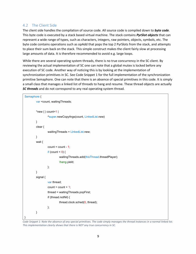
4.2 The Client Side The client side handles the compilation of source code. All source code is compiled down to byte code.
This byte code is executed by a stack based virtual machine. The stack contains PyrSlot objects that can
represent a wide range of types, such as characters, integers, raw pointers, objects, symbols, etc. The
byte code contains operations such as opAdd that pops the top 2 PyrSlots from the stack, and attempts
to place their sum back on the stack. This simple construct makes the client fairly slow at processing
large amounts of data. It is therefore recommended to avoid e.g. large loops.
While there are several operating system threads, there is no true concurrency in the SC client. By
reviewing the actual implementation of SC one can note that a global mutex is locked before any
execution of SC code. Another way of noticing this is by looking at the implementation of
synchronization primitives in SC. See Code Snippet 1 for the full implementation of the synchronization
primitive Semaphore. One can note that there is an absence of special primitives in this code. It is simply
a small class that manages a linked list of threads to hang and resume. These thread objects are actually
SC threads and do not correspond to any real operating system thread.
Semaphore {
var <count, waitingThreads;
*new { | count=1 |
^super.newCopyArgs(count, LinkedList.new)
}
clear {
waitingThreads = LinkedList.new;
}
wait {
count = count - 1;
if (count < 0) {
waitingThreads.add(thisThread.threadPlayer);
\hang.yield;
};
}
signal {
var thread;
count = count + 1;
thread = waitingThreads.popFirst;
if (thread.notNil) {
thread.clock.sched(0, thread);
};
}
}
Code Snippet 1: Note the absence of any special primitives. The code simply manages the thread instances in a normal linked list. This implementation clearly shows that there is NOT any true concurrency in SC.
10
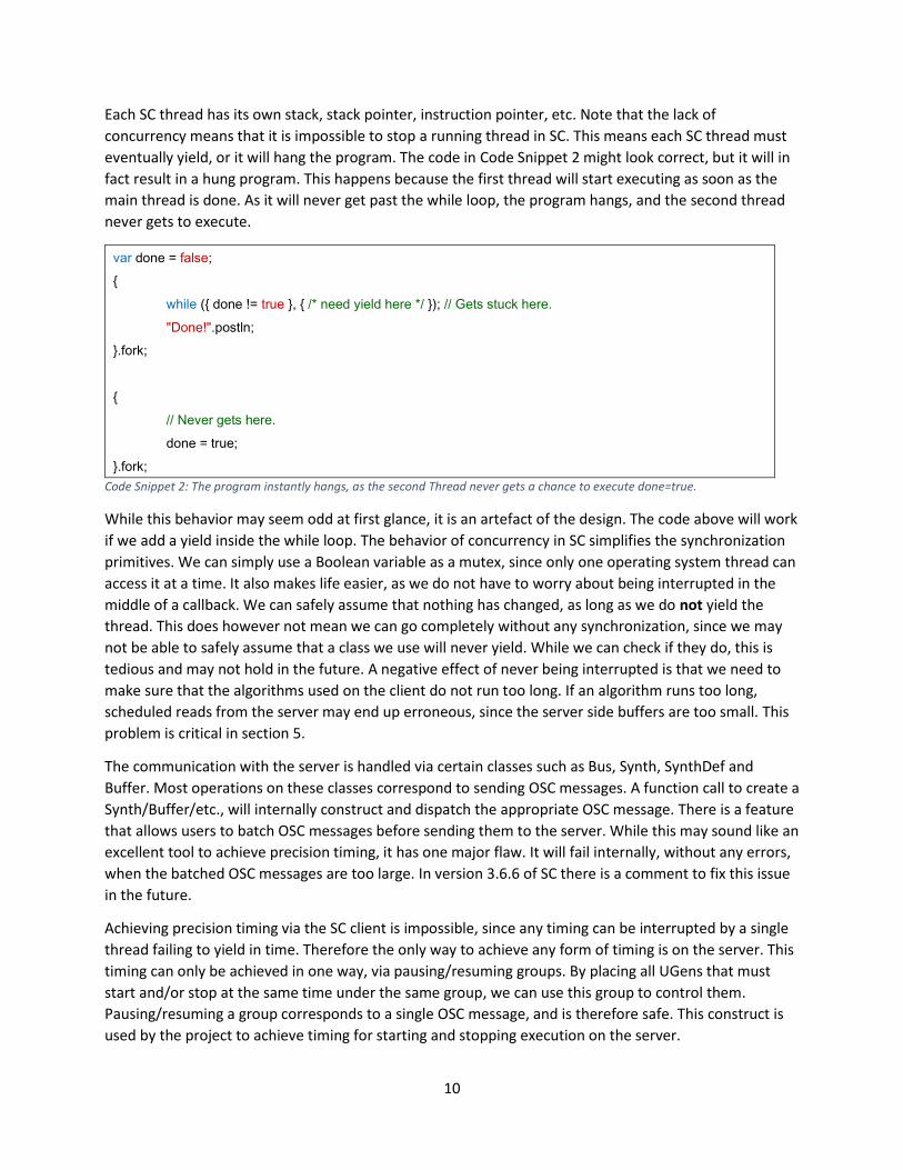
Each SC thread has its own stack, stack pointer, instruction pointer, etc. Note that the lack of
concurrency means that it is impossible to stop a running thread in SC. This means each SC thread must
eventually yield, or it will hang the program. The code in Code Snippet 2 might look correct, but it will in
fact result in a hung program. This happens because the first thread will start executing as soon as the
main thread is done. As it will never get past the while loop, the program hangs, and the second thread
never gets to execute.
var done = false;
{
while ({ done != true }, { /* need yield here */ }); // Gets stuck here.
"Done!".postln;
}.fork;
{
// Never gets here.
done = true;
}.fork;
Code Snippet 2: The program instantly hangs, as the second Thread never gets a chance to execute done=true.
While this behavior may seem odd at first glance, it is an artefact of the design. The code above will work
if we add a yield inside the while loop. The behavior of concurrency in SC simplifies the synchronization
primitives. We can simply use a Boolean variable as a mutex, since only one operating system thread can
access it at a time. It also makes life easier, as we do not have to worry about being interrupted in the
middle of a callback. We can safely assume that nothing has changed, as long as we do not yield the
thread. This does however not mean we can go completely without any synchronization, since we may
not be able to safely assume that a class we use will never yield. While we can check if they do, this is
tedious and may not hold in the future. A negative effect of never being interrupted is that we need to
make sure that the algorithms used on the client do not run too long. If an algorithm runs too long,
scheduled reads from the server may end up erroneous, since the server side buffers are too small. This
problem is critical in section 5.
The communication with the server is handled via certain classes such as Bus, Synth, SynthDef and
Buffer. Most operations on these classes correspond to sending OSC messages. A function call to create a
Synth/Buffer/etc., will internally construct and dispatch the appropriate OSC message. There is a feature
that allows users to batch OSC messages before sending them to the server. While this may sound like an
excellent tool to achieve precision timing, it has one major flaw. It will fail internally, without any errors,
when the batched OSC messages are too large. In version 3.6.6 of SC there is a comment to fix this issue
in the future.
Achieving precision timing via the SC client is impossible, since any timing can be interrupted by a single
thread failing to yield in time. Therefore the only way to achieve any form of timing is on the server. This
timing can only be achieved in one way, via pausing/resuming groups. By placing all UGens that must
start and/or stop at the same time under the same group, we can use this group to control them.
Pausing/resuming a group corresponds to a single OSC message, and is therefore safe. This construct is
used by the project to achieve timing for starting and stopping execution on the server.

11
A SynthDef is a template for a Synth on the server side. It consists of a function that can utilize UGens to
complete its task. The SynthDefs takes parameters, usually these consist of constants, buses and/or
buffers. Once a SynthDef has been sent to the server, and been fully compiled, we can request to
instantiate these Synths using the SynthDef as a template. The Synth takes the parameters handed to the
SynthDef, as well as instructions on where to place the final Synth in the tree on the server side. The first
time the Synth is computed on the server, its UGens constructors are called, and then the first iteration
of their calculation functions. The SynthDef is written in SC, the code examples in section 6.1 and 6.2
corresponds to such SynthDefs.
While plugins can be made in the form of UGens for the server side, the same support is not yet available
for the client. Primitives do exist on the client, as small indivisible operations, but these are hardcoded
into the source for the entire client. Hence, new primitives can be added on the client side, but will
require a complete re-compilation of the entire SC client, and is therefore tedious to install on different
machines. Note that this effectively is a modification of the SC client rather than a plugin.
Although new primitives are tedious to make for the client, it is important to utilize the ones that are
already there. Primitives in SC always begin with an underscore. This can be seen in Table 1, based on
the three versions formatting data as a matrix from Code Snippet 3. Since it is not trivial how to measure
time in SC, this was also included in Code Snippet 3. There are many ways of grabbing the current
timestamp, however Process.elapsedTime is the only one that always grabs an updated timestamp, since
it maps directly to the primitive _ElapsedTime.
(
var arr = Array.iota(100000);
var time = Process.elapsedTime;
100 do: {
var n = 5;
var m = (arr.size / n).asInteger;
arr.unlace(n); // Version 1
n collect: { | k | arr[ Array.series(m, k, n) ] }; // Version 2
n collect: { | k | Array.series(m, k, n) collect: { | i | arr[i] } }; // Version 3
nil
};
format("Time: %", Process.elapsedTime - time).postln;
)
Code Snippet 3: Three versions formatting 100000 integers as a matrix. Time measurement is also shown in the above example.
Version Description Time (s)
1 Directly maps to the primitive _ArrayUnlace. 0.031
2 Utilizes the primitive _BasicAt to create the subarray. 1.134
3 Not attempting to utilize any primitives. 2.952
Table 1: Comparison between utilizing and avoiding primitives to format data as a matrix.

12
It is clear to see that utilizing primitives plays a major part in efficiency on the SC client, since it can boost
performance significantly. It can also be seen that it is always preferable to find a primitive that does
exactly what is required. Version 2 is barely faster than version 3 since the majority of the time is spent
on constructing the array with indices into arr.
13
5 Data Transfer There are two types of data transfer used by the project. First and foremost we need to get the data
from the server to the client to present it in the graphical user interface. Since the purpose of this project
is to evaluate the method, described in section 2, we also need to transfer this data to programs such as
MATLAB. Thus, we need to write the results to disk.
5.1 Server to Client Since the main purpose of this project is to give direct feedback to the user, we need to present the data
in real time. Thus, it is critical to get the data from the server (where it is computed) to the client (where
we can present it).
5.1.1 Problem In the given prototype, OSC messages were sent to the server to grab results from control rate buses at a
specific rate. This resulted in a “rough undersampling” of the output from the server, which was one of
the biggest issues with the given prototype. A separate problem was caused by calculations being
performed in pseudo demand rate using control rate, rather than audio rate. This meant that an input
EGG signal with a frequency of more than 689 Hz, on a typical machine with default settings, resulted in
lost data. Such high frequencies are typically rare, but can still cause trouble, so it required a fix.
5.1.2 Trivial Solution? The problem with the pseudo demand rate construct can easily be avoided by using audio rate rather
than control rate. This includes all buses being upgraded to audio rate, as well as all UGens. Changing all
buses to audio rate was not entirely possible, since there were stock UGens in use that do not support
audio rate. These perform estimations of frequency, crest factor, amplitude and clarity. Since these are
estimations depending solely on the incoming audio signal, the fact that they run only at control rate was
not seen as a problem.
In SC the typical way to solve the second problem is to avoid it altogether. This can be done by letting the
server build the exact representation required by the client to present it. An example of such a solution
can be seen with the built in scopes. These use a fixed size buffer on the server. Depending on the size of
the scope, it may use interpolation on the server, but typically it only updates the scope by adding new
data and discarding expired data. However, as explained towards the end of section 4.1, transferring
data from the server to the client is included in the control period. Thus, if the representation requires
frequent updates on the client, it is vital that the representation is sufficiently small. Further, the
graphical user interface requires special constructs such as a color and position. This means that the data
from the server cannot directly be pushed to the graphical user interface on the client, but needs to be
converted first. This means that the representation required by the client must be very small for such a
solution to work.
The VRP data, which is formatted as a matrix of colors, contains the most information. The data consists
of several matrices, one for each of the various ways to look at the VRP data. In the worst case scenario
(based on limitations on parameters) we would have 24 matrices with RGB-colors. Based on granularity
requirements the realistic size of each matrix is roughly 200x200, but can be as large as 500x500. With 24
matrices with 500x500 RGB-colors, we would have to transfer 18 million floats on each update. We can
reduce this by only allowing one matrix to be presented at a time. Further, we can avoid representing
the data as RGB-colors on the server. Even with these improvements, we still end up with 250000 floats
14
per update. Assuming 24 updates per second to keep the visuals fluent, we end up with 6 million floats
per second. Note that we also need to convert these 250000 floats into a matrix of colors before we can
present it on the client. This requires a construct very similar to that of version 3 in Code Snippet 3 on
page 11. As seen in Table 1 on the same page, this construct takes ~30 milliseconds to convert 100000
floats into a matrix format. Thus, direct transfer of fully prepared VRP matrices from the server is not
feasible.
5.1.3 Streaming Data In order to get the data for the VRP to the client, we need to use streaming. To stream data from the
buses on the server to the client, we need to overcome some problems. Since the Synths are placing
their output in buses, we either have to stream the current content of the buffers, at control rate. This is
not possible, since the client has no or little control over timing as explained in section 4.2. Thus, we
need the server to store the data from the buses until the client can fetch it. This sub problem is
explained in detail in section 5.1.3.1. Since the server can be internal, local or remote we have different
ways of transferring data from the server to the client, and these are covered in section 5.1.3.2 and
5.1.3.3. Remember from section 4 that the client is controlling the server using the protocol OSC. This
means that we have asynchronous requests being sent to the server. These requests can get lost or
delayed. Thus, there exists a problem of managing requests to the server. Since this request
management is solved by carefully keeping track of each request, this problem is not covered here. Once
the data is present on the client, using it efficiently is vital for performance. By carefully following the
general hints given in section 4.2, we can avoid this problem as much as possible. Thus, this step is not
covered in this thesis.
5.1.3.1 Buffering Pseudo Demand Rate Data
The GatedBufWr is an UGen built specifically for the present project. The UGen’s main parameters are
the buffer, an input array with input signals to be written to the buffer and a gate which is used to
produce the pseudo demand rate. It takes the index into the buffer as a demand rate UGen, since there
already exists several demand rate UGens that generate series. It can also handle wrapping back to the
start by setting a final Boolean parameter. These parameters are simply transferred from the built in
UGen BufWr, which only handles control and audio rate. The difference is caused by the pseudo demand
rate. Obviously BufWr does not take any gate as a parameter, since it only handles audio or control rate
data. Secondly since GatedBufWr can handle data at any rate, it needs a true demand rate index, which
BufWr does not need. The output from the UGen is the last index written to.
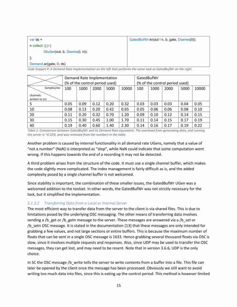
There already exists a demand rate UGen (Dbufwr) to write data into a buffer, however it has issues. The
main problem is the fact that it only can handle one input signal. While this may not sound like a big
deal, since you can simply use several Dbufwr instances to cover each input signal, it is. The first issue is
related to performance. As the number of input signals increase, the Dbufwr solution becomes
increasingly slow due to the overhead of using demand rate UGens and accessing any buffer from within
an UGen. Table 2 shows the difference in performance between GatedBufWr and the Demand rate
solution in Code Snippet 4. The table indicates that the demand rate solution scales poorly, especially if
many values are written every second. With the number of buses listened to in the present project with
typical input, this demand rate method is not a big performance issue, since it only takes up less than 1%
of the control period.
15
var ds =
n collect: { | i |
Dbufwr(out, b, Dseries(i, n));
};
Demand.ar(gate, 0, ds)
GatedBufWr.kr(out ! n, b, gate, Dseries(0));
Code Snippet 4: A Demand Rate implementation on the left that performs the same task as GatedBufWr on the right.
Demand Rate Implementation (% of the control period used)
GatedBufWr (% of the control period used)
Samples/sec
channels written to (n)
100 1000 2000 5000 10000 100 1000 2000 5000 10000
5 0.05 0.09 0.12 0.20 0.32 0.03 0.03 0.03 0.04 0.05
10 0.08 0.13 0.20 0.42 0.65 0.05 0.06 0.06 0.08 0.10
20 0.11 0.20 0.32 0.70 1.20 0.09 0.10 0.12 0.14 0.15
30 0.15 0.30 0.45 1.00 1.70 0.11 0.14 0.15 0.17 0.19
40 0.19 0.40 0.60 1.40 2.30 0.14 0.16 0.17 0.19 0.22 Table 2: Comparison between GatedBufWr and its Demand Rate equivalent. The overhead from generating data, and running the server is ~0.32%, and was removed from the numbers in the table.
Another problem is caused by internal functionality in all demand rate UGens, namely that a value of
“not a number” (NaN) is interpreted as “stop”, while NaN could indicate that some computation went
wrong. If this happens towards the end of a recording it may not be detected.
A third problem arises from the structure of the code. It must use a single channel buffer, which makes
the code slightly more complicated. The index management is fairly difficult as is, and the added
complexity posed by a single channel buffer is not welcomed.
Since stability is important, the combination of these smaller issues, the GatedBufWr UGen was a
welcomed addition to the toolset. In other words, the GatedBufWr was not strictly necessary for the
task, but it simplified the implementation.
5.1.3.2 Transferring Data from a Local or Internal Server
The most efficient way to transfer data from the server to the client is via shared files. This is due to
limitations posed by the underlying OSC messaging. The other means of transferring data involves
sending a /b_get or /b_getn message to the server. These messages are answered via a /b_set or
/b_setn OSC message. It is stated in the documentation [13] that these messages are only intended for
grabbing a few values, and not large sections or entire buffers. This is because the maximum number of
floats that can be sent in a single OSC message is 1633. Hence grabbing several thousand floats via OSC is
slow, since it involves multiple requests and responses. Also, since UDP may be used to transfer the OSC
messages, they can get lost, and may need to be resent. Note that in version 3.6.6, UDP is the only
choice.
In SC the OSC message /b_write tells the server to write contents from a buffer into a file. This file can
later be opened by the client once the message has been processed. Obviously we still want to avoid
writing too much data into files, since this is eating up the control period. This method is however limited

16
by the hard drive where the files are stored. In specific situations, with very little data being transferred,
/b_getn may be superior. Such specific optimizations are however not considered for this master thesis.
There exists a function in the Buffer class that sends a /b_write message to the server, and later grabs
the data on the client (as an array). This function is called loadToFloatArray, and works well for most
situations. It does not work for transferring data for the BusListener implementation. loadToFloatArray
names the shared file via taking the hash value of the Buffer instance. The BusListener implementation
can manage several requests in parallel. This feature is used in the situation where the data is wrapped
around the end of the buffer or after lost requests. Remember that /b_write is not free from failure,
since this message can get lost, especially in situations with high contention. This brings us to the next
problem with loadToFloatArray: it assumes success. If the file does not exist, indicating that the server
never actually got the /b_write OSC message, an empty float array will be returned. This float array will
then be passed to the “success handler”, while it actually failed internally. Also, there are no checks for
bad files; for example an old file from a previous read. This flaw makes the function especially prone to
silent (hard to debug) failures. Finally sending multiple requests with loadToFloatArray is difficult, since it
will synchronize with the server, which has an effect of temporarily suspending the current SC thread
until the server has processed the /b_write OSC message. While it may sound like multiple parallel
requests are impossible, they are not. These must simply be requested from different SC threads, and
land on the server in the same control period. When two /b_write OSC messages tell the server to write
different data into the same file, it obviously results in hard to debug errors when the client reads from
this file.
All of the issues with loadToFloatArray were fixed by adding a similar feature, called
“MultiLoadToFloatArray”. This feature is a part of the BufferRequester machinery produced especially
for the present project. It includes the starting position for the read, as well as the length of the read in
the filename. This makes several parallel reads possible. All /b_write messages are bundled together
before being sent to the server, which means that multiple parallel requests can be made with only one
sync, which improves efficiency. The implementation will also verify that the file exists and that its
content has the expected size. This results in a much more robust and versatile version of
loadToFloatArray.
5.1.3.3 Transferring Data from a Remote Server
With a remote server, the only way to transfer buffer data from the server to the client is via /b_getn
messages. As described in the previous section the server will respond with a matching /b_setn message,
including the read data. This message can at most transfer 1633 floats per read, which means that many
messages may be necessary to transfer the buffers contents. The probability of losing packets is also
increased with a remote server, since it must travel over the network. Splitting a larger request into
smaller ones is the main problem with utilizing /b_getn. Any of the requests may get lost, and may end
up in the wrong order. This complexity means that the client must work harder to ensure correctness in
the retrieved results.
17
5.2 Server to File Writing the results to a file is important for several reasons. Since the project’s main purpose is research,
it is important to be able to store any recordings and presented results in files, so that these results can
be loaded into e.g. MATLAB. SC already has a few different ways of writing data to files. First and
foremost we can write the contents of an entire buffer into a sound file via /b_write. It is however not
always possible to store the results in a fixed size buffer. Hence, it is required to stream data into a file, a
small chunk at a time. This can be achieved via using the UGen DiskOut in SC. The DiskOut UGen is
however limited to only writing audio rate signals. In the present project we have output at two different
rates. We do have signals at audio rate, namely the gates and echoed or preprocessed input signals. For
this section the cycle rate will also be coined. This rate is posed by the ever changing rate of good EGG
cycles. Thus, in order to utilize DiskOut we would have to repeat the information at this cycle rate. This is
hugely inefficient since it is required to output points, and many different measurements. As a maximum
limit we can output 114 channels at audio rate. Many of these values are however related, and thus it is
unrealistic to write all channels to a file. Even if we cut the number of output channels in half, with
minimal redundancy, we still have a huge amount of output. Remember that each of these channels
would provide us with 44100 samples per second on a typical machine. Each sample would require 2-4
bytes to be stored on disk. With 62 channels and 44100 samples per second with 2 bytes per sample we
end up at ~5.2 MB/s worth of data. Thus, it was vital to make a new UGen that could reduce this
redundancy via splitting up the results into two files. One file at cycle rate and the other at audio rate.
The DiskOut UGen has got a few undocumented flaws, which are fixed in the GatedDiskOut UGen built
for the present project. A quite fatal flaw in the design of DiskOut is its reliance on an internal array on
the stack. This array has the fixed size of 32, which is defined as the maximum number of channels
internally. The documentation for this UGen does not mention this, and the UGen simply crashes if more
channels are added. This internal limit was removed in the GatedDiskOut UGen, and is now only posed
by the output file type and the upper limit on the number of parameters to an UGen (64). Another
problem with DiskOut is noticeable at the end of a recording, namely that it might throw away one or
several seconds of the recording. This flaw is caused by the way the UGen is forced to work internally.
Since it cannot write data to the file every control period it rather gathers samples until it reaches above
a limit before it writes it to the file. This number can be controlled by the user via the size of the buffer. It
is however not safe to use a small buffer, since the UGen cannot write directly to the file. Remember
from section 4.1 that the UGens run in the real time (RT) context, and are thus prohibited to run any file
I/O. Thus, the UGen simply dispatches a message to write to the file in the non-real time (NRT) context.
We lose samples because the UGen buffers up one or several seconds worth of samples before it sends
such a message to the NRT context. This message is however not sent in the UGens destructor, which is
called as the UGen is freed. Thus, any data still left in the internal buffer is simply lost. This problem was
prevented in the GatedDiskOut UGen via sending a message to the NRT context in the destructor. There
was however still one more problem. Remember that a message was sent to the NRT thread, and thus
we are performing an asynchronous write to the file. We can wait until the UGen has been freed before
we close the file, but this is not entirely safe, since the write might be in progress or not yet initiated in
the NRT context. In order to safely be able to free the buffer we would require a special sync command
that we can send from the client. This command could then let us sync with the final write to the file.
Due to the time constraints on this project, the implemented solution simply waits for one second after
the UGen has been freed before freeing the buffer and closing the file. This should be plenty of time for
the NRT context to finish the final write.

18
Appendix A contains a detailed explanation of the connection between the two different types of output
files.

19
6 Cycle Separation This section focuses on the cycle separation, the first true step of the algorithm, see section 2 if you need
a recap on its purpose. The input to the cycle separation is the preprocessed EGG signal. This EGG signal
is assumed to be periodic. The task of the cycle separation is to separate the EGG signal into suitable
periods. During the work with the method, two different ways of performing cycle separation were
tested. The first utilized phase portraits, and the second used the so called “peak-follower” paradigm
[14]. These algorithms will be explained in detail in section 6.1 and 6.2. Earlier comparisons between the
two have been made [11], but this comparison was fairly limited. Since the cycle separation is vital for
the rest of the method, a comparative analysis was carried out. See section 6.3 for details on how this
comparison was done. Section 6.4 presents the results and sections 6.5 and 6.6 present an analysis of
the results and makes a conclusion.
6.1 Phase Portrait The phase portrait algorithm works by looking for complete revolutions in the graph produced by the
function 𝑦𝑗, where ℋ(𝑥𝑗) denotes the Hilbert transform of 𝑥𝑗, where 𝑥𝑗 is sample 𝑗 of the preprocessed
EGG signal.
𝑦𝑗 = 𝑥𝑗 + 𝑖ℋ(𝑥𝑗)
This will produce a circular path in the complex plane. Once a full revolution has passed, a new cycle
starts. The algorithm behaved poorly in the initial tests performed by [11], although the implementation
used in those tests worked slightly differently when converting the Hilbert signal into a “trigger”. A
trigger is a signal, which notifies an UGen that something should happen, when it changes its sign from
negative to positive. Due to the earlier studies by [11] it is expected that this algorithm will be inferior in
comparison to the double sided peak follower.
hilbert = Hilbert.ar(rawEGG)[1];
// atan2 gives output in the range [-pi, +pi], we change this to [2pi - epsilon, -epsilon] so it can work as a trigger.
z = Trig1.ar( atan2(hilbert, inLP).linlin(pi.neg, pi, 2*pi - epsilon, epsilon.neg), 0 );
Code Snippet 5: The implementation of the Phase Portrait. rawEGG is the raw EGG signal.
6.2 Peak Follower Note that the author of this thesis has not participated in the development of the peak follower
implementation.
A peak follower works by following the signals to every peak, and then decaying down towards it as it
drops. This produces a new signal, the peak follower signal. This can then be used to detect cycles. See
Figure 4 for an example of a peak follower signal. In SC we can control the rate of decay 𝜀. The decay
parameter controls how quickly the peak follower signal drops towards the input signal. This is done
according to the function
𝑦𝑡 = {𝑥𝑡 𝑖𝑓 𝑥𝑡 > 𝑥𝑡−1
𝑥𝑡 − 𝜀(𝑥𝑡−1 − 𝑥𝑡) 𝑜𝑡ℎ𝑒𝑟𝑤𝑖𝑠𝑒
where 𝑦𝑡 is a sample of the peak follower signal and 𝑥𝑡 a sample of the input signal at time 𝑡. This signal
can then be used in a trigger. In SC we have the trigger UGen Trig1 that works by outputting zeros until
its trigger signal changes sign from negative to positive. Once this takes place, it will output ones for a
20
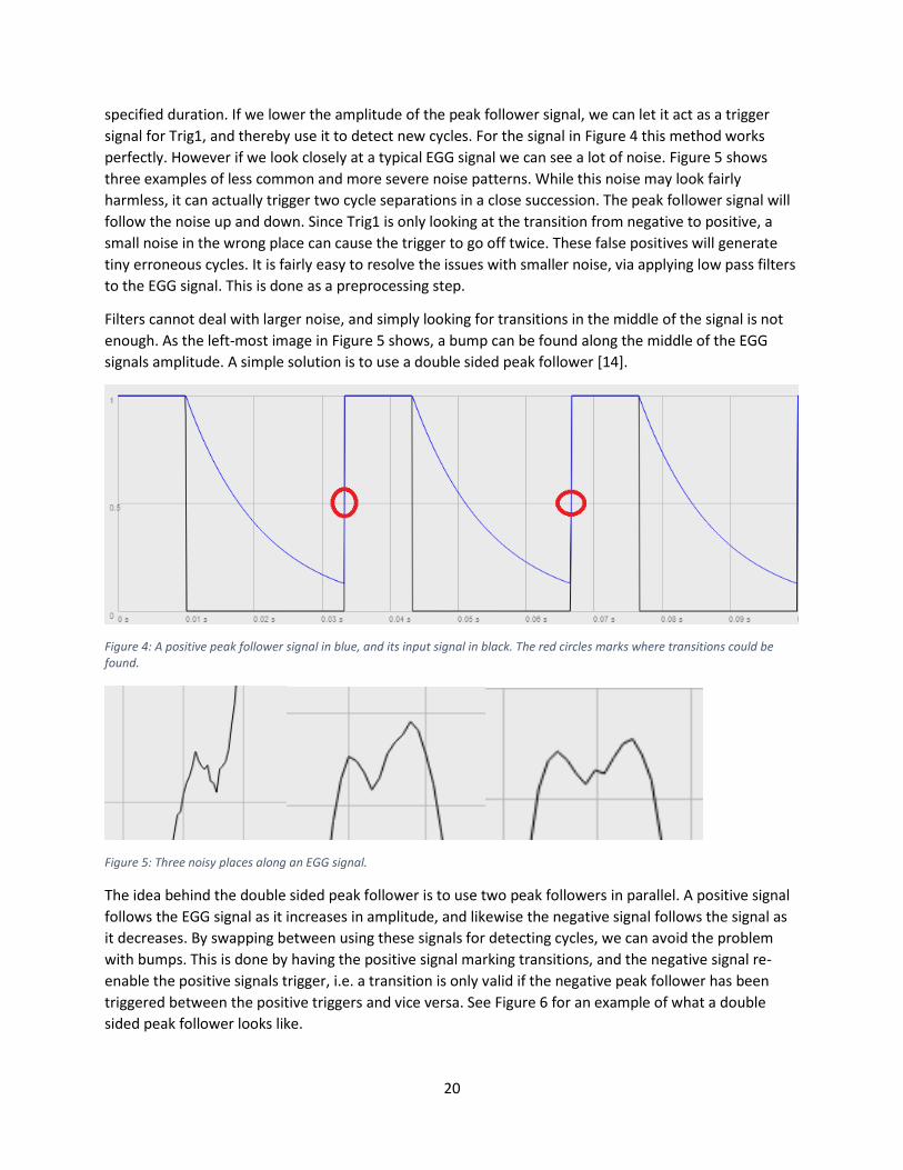
specified duration. If we lower the amplitude of the peak follower signal, we can let it act as a trigger
signal for Trig1, and thereby use it to detect new cycles. For the signal in Figure 4 this method works
perfectly. However if we look closely at a typical EGG signal we can see a lot of noise. Figure 5 shows
three examples of less common and more severe noise patterns. While this noise may look fairly
harmless, it can actually trigger two cycle separations in a close succession. The peak follower signal will
follow the noise up and down. Since Trig1 is only looking at the transition from negative to positive, a
small noise in the wrong place can cause the trigger to go off twice. These false positives will generate
tiny erroneous cycles. It is fairly easy to resolve the issues with smaller noise, via applying low pass filters
to the EGG signal. This is done as a preprocessing step.
Filters cannot deal with larger noise, and simply looking for transitions in the middle of the signal is not
enough. As the left-most image in Figure 5 shows, a bump can be found along the middle of the EGG
signals amplitude. A simple solution is to use a double sided peak follower [14].
Figure 4: A positive peak follower signal in blue, and its input signal in black. The red circles marks where transitions could be found.
Figure 5: Three noisy places along an EGG signal.
The idea behind the double sided peak follower is to use two peak followers in parallel. A positive signal
follows the EGG signal as it increases in amplitude, and likewise the negative signal follows the signal as
it decreases. By swapping between using these signals for detecting cycles, we can avoid the problem
with bumps. This is done by having the positive signal marking transitions, and the negative signal re-
enable the positive signals trigger, i.e. a transition is only valid if the negative peak follower has been
triggered between the positive triggers and vice versa. See Figure 6 for an example of what a double
sided peak follower looks like.
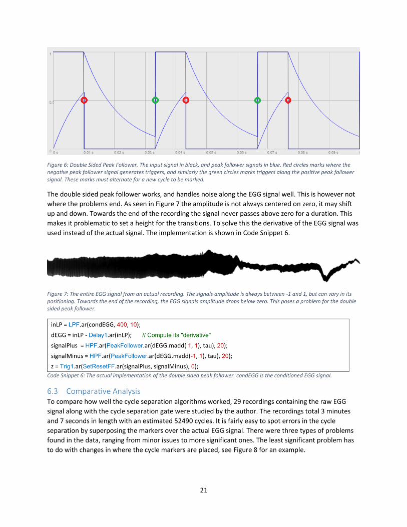
21
Figure 6: Double Sided Peak Follower. The input signal in black, and peak follower signals in blue. Red circles marks where the negative peak follower signal generates triggers, and similarly the green circles marks triggers along the positive peak follower signal. These marks must alternate for a new cycle to be marked.
The double sided peak follower works, and handles noise along the EGG signal well. This is however not
where the problems end. As seen in Figure 7 the amplitude is not always centered on zero, it may shift
up and down. Towards the end of the recording the signal never passes above zero for a duration. This
makes it problematic to set a height for the transitions. To solve this the derivative of the EGG signal was
used instead of the actual signal. The implementation is shown in Code Snippet 6.
Figure 7: The entire EGG signal from an actual recording. The signals amplitude is always between -1 and 1, but can vary in its positioning. Towards the end of the recording, the EGG signals amplitude drops below zero. This poses a problem for the double sided peak follower.
inLP = LPF.ar(condEGG, 400, 10);
dEGG = inLP - Delay1.ar(inLP); // Compute its "derivative"
signalPlus = HPF.ar(PeakFollower.ar(dEGG.madd( 1, 1), tau), 20);
signalMinus = HPF.ar(PeakFollower.ar(dEGG.madd(-1, 1), tau), 20);
z = Trig1.ar(SetResetFF.ar(signalPlus, signalMinus), 0);
Code Snippet 6: The actual implementation of the double sided peak follower. condEGG is the conditioned EGG signal.
6.3 Comparative Analysis To compare how well the cycle separation algorithms worked, 29 recordings containing the raw EGG
signal along with the cycle separation gate were studied by the author. The recordings total 3 minutes
and 7 seconds in length with an estimated 52490 cycles. It is fairly easy to spot errors in the cycle
separation by superposing the markers over the actual EGG signal. There were three types of problems
found in the data, ranging from minor issues to more significant ones. The least significant problem has
to do with changes in where the cycle markers are placed, see Figure 8 for an example.
22
Figure 8: Showing changes in where cycle markers (as red vertical lines) are placed along the EGG signal (in black). On the left hand side markers are placed in the center of downhill slopes, whereas they are placed further up on the right hand side of the image. This is a minor issue, since the algorithm only uses the DFT of the signal between these markers.
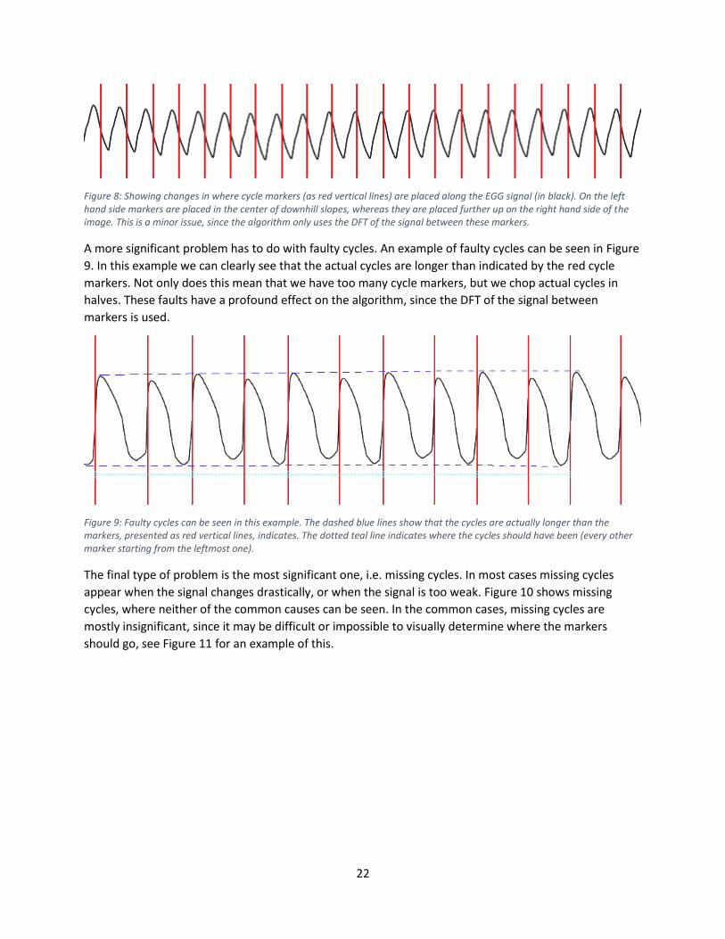
A more significant problem has to do with faulty cycles. An example of faulty cycles can be seen in Figure
9. In this example we can clearly see that the actual cycles are longer than indicated by the red cycle
markers. Not only does this mean that we have too many cycle markers, but we chop actual cycles in
halves. These faults have a profound effect on the algorithm, since the DFT of the signal between
markers is used.
Figure 9: Faulty cycles can be seen in this example. The dashed blue lines show that the cycles are actually longer than the markers, presented as red vertical lines, indicates. The dotted teal line indicates where the cycles should have been (every other marker starting from the leftmost one).
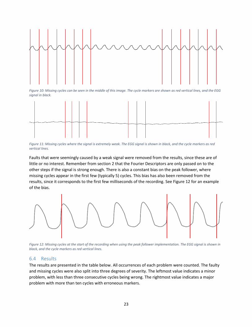
The final type of problem is the most significant one, i.e. missing cycles. In most cases missing cycles
appear when the signal changes drastically, or when the signal is too weak. Figure 10 shows missing
cycles, where neither of the common causes can be seen. In the common cases, missing cycles are
mostly insignificant, since it may be difficult or impossible to visually determine where the markers
should go, see Figure 11 for an example of this.
23
Figure 10: Missing cycles can be seen in the middle of this image. The cycle markers are shown as red vertical lines, and the EGG signal in black.
Figure 11: Missing cycles where the signal is extremely weak. The EGG signal is shown in black, and the cycle markers as red vertical lines.
Faults that were seemingly caused by a weak signal were removed from the results, since these are of
little or no interest. Remember from section 2 that the Fourier Descriptors are only passed on to the
other steps if the signal is strong enough. There is also a constant bias on the peak follower, where
missing cycles appear in the first few (typically 5) cycles. This bias has also been removed from the
results, since it corresponds to the first few milliseconds of the recording. See Figure 12 for an example
of the bias.
Figure 12: Missing cycles at the start of the recording when using the peak follower implementation. The EGG signal is shown in black, and the cycle markers as red vertical lines.
6.4 Results The results are presented in the table below. All occurrences of each problem were counted. The faulty
and missing cycles were also split into three degrees of severity. The leftmost value indicates a minor
problem, with less than three consecutive cycles being wrong. The rightmost value indicates a major
problem with more than ten cycles with erroneous markers.
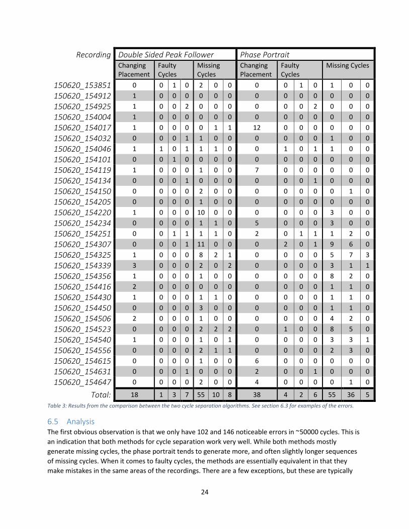
24
Recording Double Sided Peak Follower Phase Portrait Changing Placement
Faulty Cycles
Missing Cycles
Changing Placement
Faulty Cycles
Missing Cycles
150620_153851 0 0 1 0 2 0 0 0 0 1 0 1 0 0
150620_154912 1 0 0 0 0 0 0 0 0 0 0 0 0 0
150620_154925 1 0 0 2 0 0 0 0 0 0 2 0 0 0
150620_154004 1 0 0 0 0 0 0 0 0 0 0 0 0 0
150620_154017 1 0 0 0 0 1 1 12 0 0 0 0 0 0
150620_154032 0 0 0 1 1 0 0 0 0 0 0 1 0 0
150620_154046 1 1 0 1 1 1 0 0 1 0 1 1 0 0
150620_154101 0 0 1 0 0 0 0 0 0 0 0 0 0 0
150620_154119 1 0 0 0 1 0 0 7 0 0 0 0 0 0
150620_154134 0 0 0 1 0 0 0 0 0 0 1 0 0 0
150620_154150 0 0 0 0 2 0 0 0 0 0 0 0 1 0
150620_154205 0 0 0 0 1 0 0 0 0 0 0 0 0 0
150620_154220 1 0 0 0 10 0 0 0 0 0 0 3 0 0
150620_154234 0 0 0 0 1 1 0 5 0 0 0 3 0 0
150620_154251 0 0 1 1 1 1 0 2 0 1 1 1 2 0
150620_154307 0 0 0 1 11 0 0 0 2 0 1 9 6 0
150620_154325 1 0 0 0 8 2 1 0 0 0 0 5 7 3
150620_154339 3 0 0 0 2 0 2 0 0 0 0 3 1 1
150620_154356 1 0 0 0 1 0 0 0 0 0 0 8 2 0
150620_154416 2 0 0 0 0 0 0 0 0 0 0 1 1 0
150620_154430 1 0 0 0 1 1 0 0 0 0 0 1 1 0
150620_154450 0 0 0 0 3 0 0 0 0 0 0 1 1 0
150620_154506 2 0 0 0 1 0 0 0 0 0 0 4 2 0
150620_154523 0 0 0 0 2 2 2 0 1 0 0 8 5 0
150620_154540 1 0 0 0 1 0 1 0 0 0 0 3 3 1
150620_154556 0 0 0 0 2 1 1 0 0 0 0 2 3 0
150620_154615 0 0 0 0 1 0 0 6 0 0 0 0 0 0
150620_154631 0 0 0 1 0 0 0 2 0 0 1 0 0 0
150620_154647 0 0 0 0 2 0 0 4 0 0 0 0 1 0
Total: 18 1 3 7 55 10 8 38 4 2 6 55 36 5
Table 3: Results from the comparison between the two cycle separation algorithms. See section 6.3 for examples of the errors.
6.5 Analysis The first obvious observation is that we only have 102 and 146 noticeable errors in ~50000 cycles. This is
an indication that both methods for cycle separation work very well. While both methods mostly
generate missing cycles, the phase portrait tends to generate more, and often slightly longer sequences
of missing cycles. When it comes to faulty cycles, the methods are essentially equivalent in that they
make mistakes in the same areas of the recordings. There are a few exceptions, but these are typically
25
covered by missing cycles for the other method. In other words, when one marks cycles faultily the other
simply avoids making any markers for that sequence. When it comes to stability in the placement of
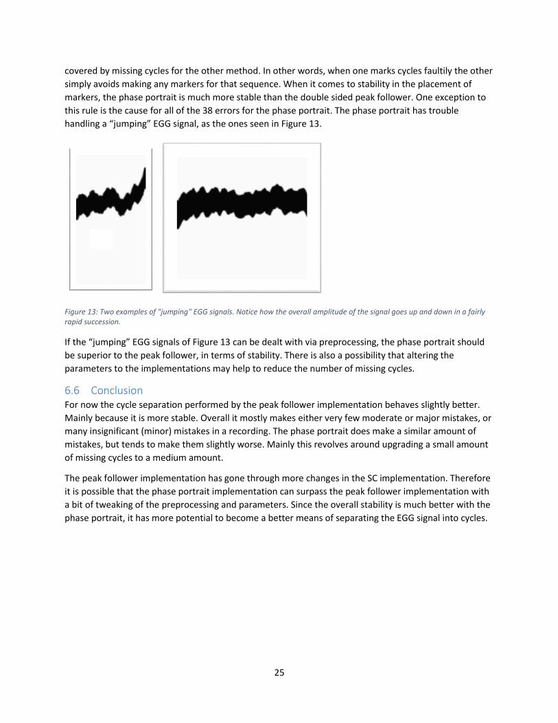
markers, the phase portrait is much more stable than the double sided peak follower. One exception to
this rule is the cause for all of the 38 errors for the phase portrait. The phase portrait has trouble
handling a “jumping” EGG signal, as the ones seen in Figure 13.
Figure 13: Two examples of "jumping" EGG signals. Notice how the overall amplitude of the signal goes up and down in a fairly rapid succession.
If the “jumping” EGG signals of Figure 13 can be dealt with via preprocessing, the phase portrait should
be superior to the peak follower, in terms of stability. There is also a possibility that altering the
parameters to the implementations may help to reduce the number of missing cycles.
6.6 Conclusion For now the cycle separation performed by the peak follower implementation behaves slightly better.
Mainly because it is more stable. Overall it mostly makes either very few moderate or major mistakes, or
many insignificant (minor) mistakes in a recording. The phase portrait does make a similar amount of
mistakes, but tends to make them slightly worse. Mainly this revolves around upgrading a small amount
of missing cycles to a medium amount.
The peak follower implementation has gone through more changes in the SC implementation. Therefore
it is possible that the phase portrait implementation can surpass the peak follower implementation with
a bit of tweaking of the preprocessing and parameters. Since the overall stability is much better with the
phase portrait, it has more potential to become a better means of separating the EGG signal into cycles.
26
7 Discrete Fourier Transform Although this portion of the algorithm has already been implemented by [11], it utilized an
approximation for the DFT calculations. This was not necessary, since there are precalculated sine
wavetables built into the SC server. In order to make use of these tables we can utilize the DFT formula
expanded with Euler’s formula along with the relationship between sine and cosine.
{
𝑋𝑘 = ∑ 𝑥𝑛𝑒
−𝑖2𝜋𝑘𝑛𝑁
𝑁−1
𝑛=0
𝑒𝑖𝜃 = cos 𝜃 + isin𝜃cos𝜃 = sin(𝜃 + 𝜋 2⁄ )
With these equations we get
𝑋𝑘 = ∑ 𝑥𝑛 (sin (𝜑 +𝜋
2) − 𝑖 sin𝜑)
𝑁−1
𝑛=0
where
𝜑 = 𝑛2𝜋𝑘
𝑁
With this new formula, we can utilize the sine wavetable, and we can avoid using any form of
approximation. A comparison against sinf in the C standard library reveals an error smaller than
5 ∗ 10−7. This is good, since the 32 bit floating point variables used in SC only offer 6 decimals of
precision. Access to the table is also highly optimized, since it is used in one of the most common UGens,
namely SinOsc.
Since performance is of essence in this project, [11] enabled a small delay when calculating the DFT
values. This delay means that the sum can be calculated one value at a time, which enables the DFT
calculations to have an even distribution of CPU usage. The UGen continuously reads new values storing
these in buffers until a full cycle has been found. Once the length of a cycle is known, we can start
calculating its DFT sum, one value at a time. This is where the new version differs, since it avoids relying
on approximations.
We can note that ϕ in the equation above only depends on n. Thus, we can pre-calculate 𝜑0 =2𝜋𝑘
𝑁 and
use it to increment ϕ as the DFT sum is computed. The implementation is slightly more complicated than
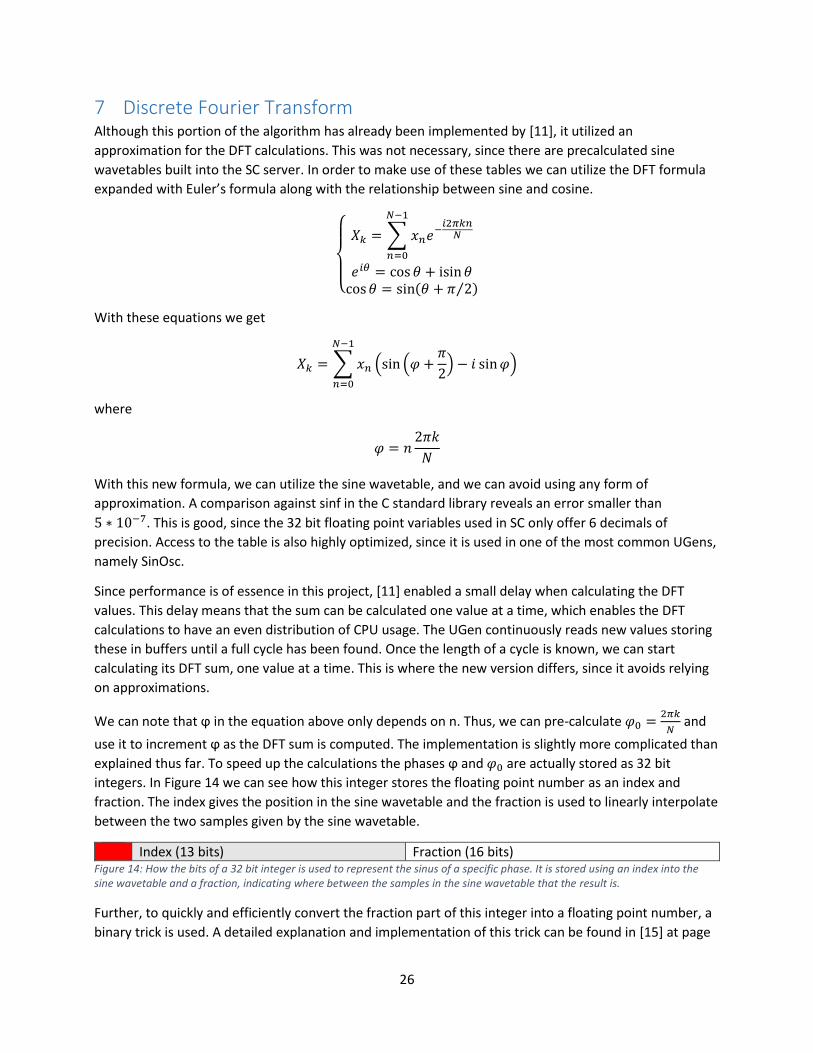
explained thus far. To speed up the calculations the phases ϕ and 𝜑0 are actually stored as 32 bit
integers. In Figure 14 we can see how this integer stores the floating point number as an index and
fraction. The index gives the position in the sine wavetable and the fraction is used to linearly interpolate
between the two samples given by the sine wavetable.
Index (13 bits) Fraction (16 bits) Figure 14: How the bits of a 32 bit integer is used to represent the sinus of a specific phase. It is stored using an index into the sine wavetable and a fraction, indicating where between the samples in the sine wavetable that the result is.
Further, to quickly and efficiently convert the fraction part of this integer into a floating point number, a
binary trick is used. A detailed explanation and implementation of this trick can be found in [15] at page

27
144. This trick is summarized in Figure 15. It places this fraction inside the representation of the mantissa
of the IEEE float. An exponent part set to 127 (indicating an exponent of zero) and a “positive” sign,
result in an IEEE float with a value between one and two.
Sign Exponent Mantissa (or fractional part)
1 bit 8 bits 23 bits
0 0111 1111 Fraction (16 bits) 0000 000
𝐼𝐸𝐸𝐸 𝐹𝑙𝑜𝑎𝑡 = (−1)𝑠𝑖𝑔𝑛 ∗ 2𝑒𝑥𝑝𝑜𝑛𝑒𝑛𝑡−127 ∗ (1 +𝑚𝑎𝑛𝑡𝑖𝑠𝑠𝑎 ∗ 2−23) = (−1)0 ∗ (1 +𝑚𝑎𝑛𝑡𝑖𝑠𝑠𝑎 ∗ 2−23) ∗ 20
= 1 + 𝑓𝑟𝑎𝑐𝑡𝑖𝑜𝑛 ∗ 2−16
Figure 15: In the table we can see how the fraction bits are placed inside the representation of the IEEE float. We can also see that the exponent’s bits are set to 127, and the sign to zero. Given the equation, we can see how this builds the IEEE float. Note that the sum this results in gets a value between one and two.
Note that adding to the 32 bit integer in Figure 14 will increment the index when the fraction wraps
around. Thus, this integer representation can fully replace the floating point representation, even for
phase shifts, until it is required by the DFT calculations.
We could store consecutive samples of a single sine wave and use this as the sine wavetable. Linear
interpolation could then be used to get values between two consecutive samples a and b using the
fraction part of the integer representation. To use linear interpolation, we would have to calculate:
sin 𝛼 = 𝑎 + (𝑓 − 1)(𝑏 − 𝑎)
We can avoid calculating (𝑓 − 1) and (𝑏 − 𝑎) via letting two samples represent something other than
two consecutive samples of the sine wave. By letting
sin𝛼 = (2𝑎 − 𝑏) + 𝑓 ∗ (𝑏 − 𝑎) = 𝑎 + (𝑓 − 1)(𝑏 − 𝑎)
we can see that this allows us to avoid the floating point subtractions by having (2𝑎 − 𝑏) and (𝑏 − 𝑎) in
the precalculated table. This table is called the sine wavetable, and is used as described earlier. By
utilizing the integer representation and the sine wavetable we can calculate the sine of any phase with
integer and binary operations, and only one floating point addition and multiplication. Thus, for each
sample in the DFT calculations we only end up with four floating point additions and multiplications. The
rest of the calculations can be done with integer and binary operations, which are faster according to
[15]:
“Simple integer operations such as addition, subtraction, comparison, bit operations
and shift operations take only one clock cycle on most microprocessors. […]Floating
point addition takes 3 - 6 clock cycles, depending on the microprocessor.
Multiplication takes 4 - 8 clock cycles.”

28
8 Sample Entropy The sample entropy calculations are used by the method (see section 2) to determine when something
significant happens to the amplitude and phase of the first few harmonics. Sample Entropy is closely
related to Approximate Entropy, and is exactly the negative natural logarithm of “the conditional
probability that two sequences within a tolerance r for m points remain within r of each other at the next
point” [16].
The sample entropy is defined [16] as follows:
𝑢 = {𝑣1, 𝑣2, 𝑣3, … , 𝑣𝑛}
𝑋𝑚(𝑖) = {𝑣𝑖, 𝑣𝑖+1, 𝑣𝑖+2, … , 𝑣𝑖+𝑚−1}
𝑑(𝑎, 𝑏) = max𝑖=1,2,3,…,|𝑎|
‖𝑎𝑖 − 𝑏𝑖‖
𝑐(𝑎, 𝑏, 𝑟) = {1 𝑖𝑓 𝑎 ≠ 𝑏 ∧ 𝑑(𝑎, 𝑏) < 𝑟
0 𝑜𝑡ℎ𝑒𝑟𝑤𝑖𝑠𝑒
𝐴𝑚𝑖(𝑟) = (𝑛 −𝑚 − 1)−1∑ 𝑐(𝑥𝑚+1(𝑖), 𝑥𝑚+1(𝑗), 𝑟)𝑛−𝑚
𝑗=1
𝐵𝑚𝑖(𝑟) = (𝑛 −𝑚 − 1)−1∑ 𝑐(𝑥𝑚(𝑖), 𝑥𝑚(𝑗), 𝑟)𝑛−𝑚
𝑗=1
𝐴𝑚(𝑟) = (𝑛 −𝑚)−1∑ 𝐴𝑚𝑖(𝑟)
𝑛−𝑚
𝑖=1
𝐵𝑚(𝑟) = (𝑛 −𝑚)−1∑ 𝐵𝑚𝑖(𝑟)
𝑛−𝑚
𝑖=1
𝑆𝑎𝑚𝑝𝑙𝑒𝐸𝑛𝑡𝑟𝑜𝑝𝑦(𝑚, 𝑟) = − ln(𝐴𝑚(𝑟)
𝐵𝑚(𝑟))
Where 𝑢 is the input vector, 𝑚 is the length of sequences to be compared and 𝑟 is the tolerance for
matches. The function 𝑐(𝑎, 𝑏, 𝑟) is a trick to avoid a difficult definition of 𝐴𝑚𝑖(𝑟) and 𝐵𝑚𝑖(𝑟), that have
to exclude 𝑖 = 𝑗 when counting the number of sequence pairs of length 𝑚 that are within 𝑟 of each
other.
8.1 Options
8.1.1 Naïve Algorithm The naïve algorithm simply calculates the sample entropy exactly as described by the algorithm above. It
loops through the possible subsequences and checks if they match.
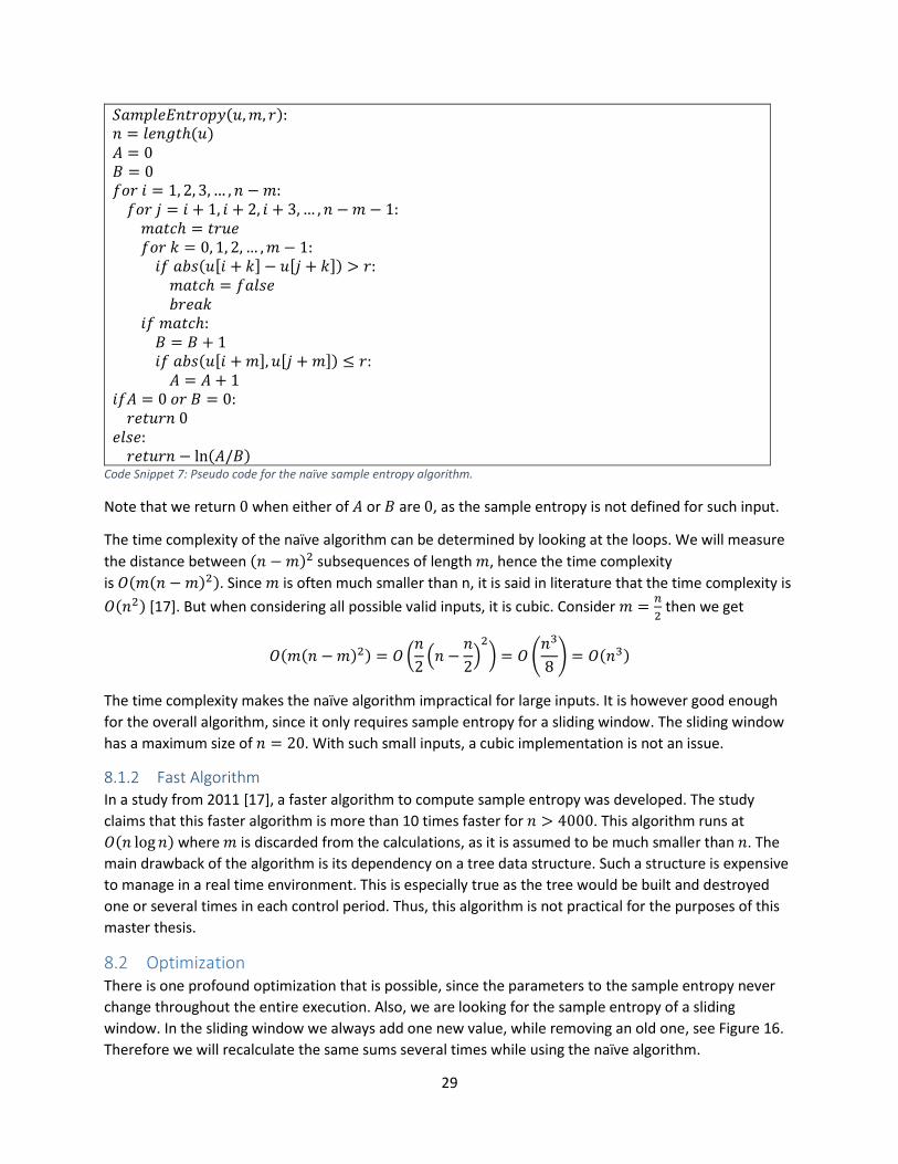
29
𝑆𝑎𝑚𝑝𝑙𝑒𝐸𝑛𝑡𝑟𝑜𝑝𝑦(𝑢,𝑚, 𝑟): 𝑛 = 𝑙𝑒𝑛𝑔𝑡ℎ(𝑢) 𝐴 = 0 𝐵 = 0 𝑓𝑜𝑟 𝑖 = 1, 2, 3, … , 𝑛 − 𝑚: 𝑓𝑜𝑟 𝑗 = 𝑖 + 1, 𝑖 + 2, 𝑖 + 3,… , 𝑛 −𝑚 − 1: 𝑚𝑎𝑡𝑐ℎ = 𝑡𝑟𝑢𝑒 𝑓𝑜𝑟 𝑘 = 0, 1, 2, … ,𝑚 − 1: 𝑖𝑓 𝑎𝑏𝑠(𝑢[𝑖 + 𝑘] − 𝑢[𝑗 + 𝑘]) > 𝑟: 𝑚𝑎𝑡𝑐ℎ = 𝑓𝑎𝑙𝑠𝑒 𝑏𝑟𝑒𝑎𝑘 𝑖𝑓 𝑚𝑎𝑡𝑐ℎ: 𝐵 = 𝐵 + 1 𝑖𝑓 𝑎𝑏𝑠(𝑢[𝑖 +𝑚], 𝑢[𝑗 + 𝑚]) ≤ 𝑟: 𝐴 = 𝐴 + 1 𝑖𝑓𝐴 = 0 𝑜𝑟 𝐵 = 0: 𝑟𝑒𝑡𝑢𝑟𝑛 0 𝑒𝑙𝑠𝑒: 𝑟𝑒𝑡𝑢𝑟𝑛 − ln(𝐴/𝐵)
Code Snippet 7: Pseudo code for the naïve sample entropy algorithm.
Note that we return 0 when either of 𝐴 or 𝐵 are 0, as the sample entropy is not defined for such input.
The time complexity of the naïve algorithm can be determined by looking at the loops. We will measure
the distance between (𝑛 − 𝑚)2 subsequences of length 𝑚, hence the time complexity
is 𝑂(𝑚(𝑛 −𝑚)2). Since 𝑚 is often much smaller than n, it is said in literature that the time complexity is
𝑂(𝑛2) [17]. But when considering all possible valid inputs, it is cubic. Consider 𝑚 =𝑛
2 then we get
𝑂(𝑚(𝑛 −𝑚)2) = 𝑂 (𝑛
2(𝑛 −
𝑛
2)2
) = 𝑂 (𝑛3
8) = 𝑂(𝑛3)
The time complexity makes the naïve algorithm impractical for large inputs. It is however good enough
for the overall algorithm, since it only requires sample entropy for a sliding window. The sliding window
has a maximum size of 𝑛 = 20. With such small inputs, a cubic implementation is not an issue.
8.1.2 Fast Algorithm In a study from 2011 [17], a faster algorithm to compute sample entropy was developed. The study
claims that this faster algorithm is more than 10 times faster for 𝑛 > 4000. This algorithm runs at
𝑂(𝑛 log 𝑛) where 𝑚 is discarded from the calculations, as it is assumed to be much smaller than 𝑛. The
main drawback of the algorithm is its dependency on a tree data structure. Such a structure is expensive
to manage in a real time environment. This is especially true as the tree would be built and destroyed
one or several times in each control period. Thus, this algorithm is not practical for the purposes of this
master thesis.
8.2 Optimization There is one profound optimization that is possible, since the parameters to the sample entropy never
change throughout the entire execution. Also, we are looking for the sample entropy of a sliding
window. In the sliding window we always add one new value, while removing an old one, see Figure 16.
Therefore we will recalculate the same sums several times while using the naïve algorithm.

30
Figure 16: How the sample entropy input is updated before the between every calculation.
With this information we only need to recalculate the number of matches for the sequences touching
the first and last element in the input range. Since we will remove the first element in the range, we
simply have to decrease the last measurement of A and B as matches are found. Similarly we add to the
previous measurement of A and B with matches containing the last element. The updated pseudo code
can be seen in Code Snippet 8.
𝑂𝑝𝑡𝑖𝑚𝑖𝑧𝑒𝑑𝑆𝑎𝑚𝑝𝑙𝑒𝐸𝑛𝑡𝑟𝑜𝑝𝑦(𝑝𝑟𝑒𝑣𝑈, 𝑝𝑟𝑒𝑣𝐴, 𝑝𝑟𝑒𝑣𝐵, 𝑢,𝑚, 𝑟): 𝑛 = 𝑙𝑒𝑛𝑔𝑡ℎ(𝑢) 𝐴 = 𝑝𝑟𝑒𝑣𝐴 𝐵 = 𝑝𝑟𝑒𝑣𝐵 𝑖𝑓 ( 𝐴 ! = 0 𝑎𝑛𝑑 𝐵 ! = 0 ) 𝑓𝑜𝑟 𝑗 = 2, 3, 4, … , 𝑛 − 𝑚 − 1: 𝑚𝑎𝑡𝑐ℎ = 𝑡𝑟𝑢𝑒 𝑓𝑜𝑟 𝑘 = 1, 2, … ,𝑚 − 1: 𝑖𝑓 𝑎𝑏𝑠(𝑝𝑟𝑒𝑣𝑈[𝑘] − 𝑝𝑟𝑒𝑣𝑈[𝑗 + 𝑘]) > 𝑟: 𝑚𝑎𝑡𝑐ℎ = 𝑓𝑎𝑙𝑠𝑒 𝑏𝑟𝑒𝑎𝑘 𝑖𝑓 𝑚𝑎𝑡𝑐ℎ: 𝐵 = 𝐵 − 1 𝑖𝑓 𝑎𝑏𝑠(𝑝𝑟𝑒𝑣𝑈[𝑚], 𝑝𝑟𝑒𝑣𝑈[𝑗 + 𝑚]) ≤ 𝑟: 𝐴 = 𝐴 − 1 𝑓𝑜𝑟 𝑗 = 0,1, 2, … , 𝑛 − 𝑚 − 1: 𝑚𝑎𝑡𝑐ℎ = 𝑡𝑟𝑢𝑒 𝑓𝑜𝑟 𝑘 = 1, 2, … ,𝑚 − 1: 𝑖𝑓 𝑎𝑏𝑠(𝑢[𝑛 − 𝑚 + 𝑘] − 𝑢[𝑗 + 𝑘]) > 𝑟: 𝑚𝑎𝑡𝑐ℎ = 𝑓𝑎𝑙𝑠𝑒 𝑏𝑟𝑒𝑎𝑘 𝑖𝑓 𝑚𝑎𝑡𝑐ℎ: 𝐵 = 𝐵 + 1 𝑖𝑓 𝑎𝑏𝑠(𝑢[𝑛], 𝑢[𝑗 + 𝑚]) ≤ 𝑟: 𝐴 = 𝐴 + 1 𝑖𝑓𝐴 = 0 𝑜𝑟 𝐵 = 0: 𝑟𝑒𝑡𝑢𝑟𝑛 0 𝑒𝑙𝑠𝑒: 𝑟𝑒𝑡𝑢𝑟𝑛 − ln(𝐴/𝐵)
Code Snippet 8: Optimized version of the naïve sample entropy algorithm.

31
If we now recalculate the time complexity, we can note that we only compare subsequences of length m
2(𝑛 −𝑚) times. Considering all possible inputs, via setting 𝑚 =𝑛
2 as before, we now have a time
complexity of:
𝑂(2(𝑛 − 𝑚)𝑚) = 𝑂(𝑛2)
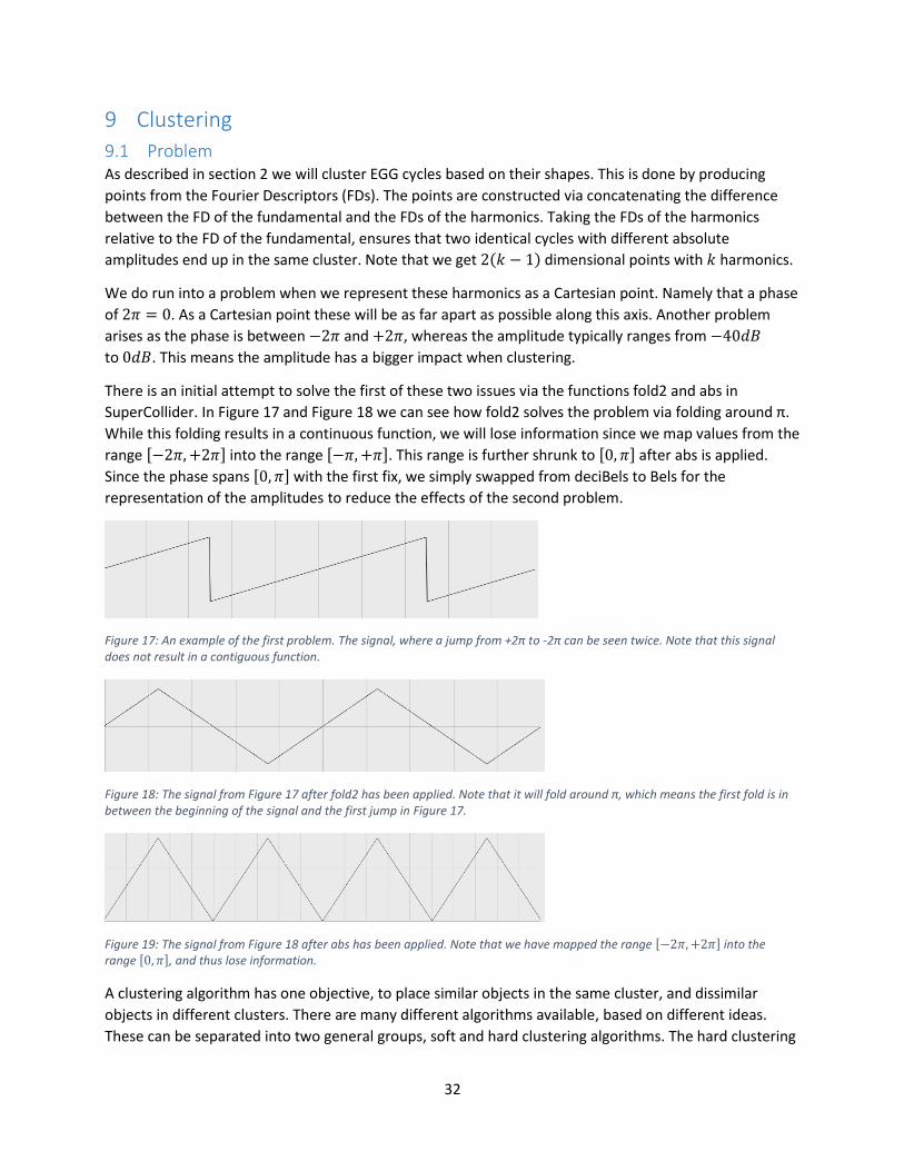
32
9 Clustering
9.1 Problem As described in section 2 we will cluster EGG cycles based on their shapes. This is done by producing
points from the Fourier Descriptors (FDs). The points are constructed via concatenating the difference
between the FD of the fundamental and the FDs of the harmonics. Taking the FDs of the harmonics
relative to the FD of the fundamental, ensures that two identical cycles with different absolute
amplitudes end up in the same cluster. Note that we get 2(𝑘 − 1) dimensional points with 𝑘 harmonics.
We do run into a problem when we represent these harmonics as a Cartesian point. Namely that a phase
of 2𝜋 = 0. As a Cartesian point these will be as far apart as possible along this axis. Another problem
arises as the phase is between −2𝜋 and +2𝜋, whereas the amplitude typically ranges from −40𝑑𝐵
to 0𝑑𝐵. This means the amplitude has a bigger impact when clustering.
There is an initial attempt to solve the first of these two issues via the functions fold2 and abs in
SuperCollider. In Figure 17 and Figure 18 we can see how fold2 solves the problem via folding around π.
While this folding results in a continuous function, we will lose information since we map values from the
range [−2𝜋,+2𝜋] into the range [−𝜋,+𝜋]. This range is further shrunk to [0, 𝜋] after abs is applied.
Since the phase spans [0, 𝜋] with the first fix, we simply swapped from deciBels to Bels for the
representation of the amplitudes to reduce the effects of the second problem.
Figure 17: An example of the first problem. The signal, where a jump from +2π to -2π can be seen twice. Note that this signal does not result in a contiguous function.
Figure 18: The signal from Figure 17 after fold2 has been applied. Note that it will fold around π, which means the first fold is in between the beginning of the signal and the first jump in Figure 17.
Figure 19: The signal from Figure 18 after abs has been applied. Note that we have mapped the range [−2𝜋,+2𝜋] into the range [0, 𝜋], and thus lose information.
A clustering algorithm has one objective, to place similar objects in the same cluster, and dissimilar
objects in different clusters. There are many different algorithms available, based on different ideas.
These can be separated into two general groups, soft and hard clustering algorithms. The hard clustering

33
algorithms work by placing each point in exactly one cluster, while the soft versions use probabilities or
scores as a measure of how much an object belongs to a cluster. A soft clustering algorithm uses more
information, as it will differentiate between an object on the edge and one in the center of a cluster.
9.2 Options We will focus on four different algorithms. All of these work by iteratively improving an initial solution to
the problem. The first three algorithms are widely used robust algorithms. All of these algorithms have
existing online equivalents [18] [19] [20]. Where online refers to the possibility of implementing the
algorithm in real time (getting one point at a time). The first algorithm is the standard K-Means
algorithm, which is both simple and robust. Following are two soft clustering algorithms, Fuzzy C-Means
and Expectation Maximization (EM) for Gaussian Mixture Models (GMMs). These two algorithms work in
different ways. EM for GMMs is focused on mathematical derivations, whereas Fuzzy C-Means is
essentially K-Means while allowing a point to belong to multiple clusters via membership degrees. We
also need to include the implementation available via SC, called KMeansRT, which is an online version of
the standard K-Means.
Let 𝑃 = {𝑥1, 𝑥2, 𝑥3, … , 𝑥𝑛} be the 𝑛 input points that should be clustered, and let 𝑆 = {𝑐1, 𝑐2, 𝑐3, … , 𝑐𝑘}
be the final 𝑘 clusters where 𝑐𝑖 ⊆ 𝑃 for 𝑖 = 1, 2, 3, … , 𝑘.
9.2.1 KMeansRT This is a description of the algorithm used in the SuperCollider UGen KMeansRT [21], brought in a set of
extra UGens for SuperCollider. The algorithm is similar to K-Means in that it keeps track of the means 𝑀,
but that is where the similarities end. KMeansRT does not store, and therefore does not remember the
input points. It is important to note that KMeansRT gets one point 𝑥𝑖 at a time, unlike the other
algorithms, that get a full set of points 𝑃. It manages a matrix that holds the means 𝑀 and member
counts 𝐶 for the clusters. As the algorithm is oblivious of earlier points on each update, it cannot take
advantage of those points in its calculations. The reason KMeansRT works in this way is because it gets
several hundred points per second as input, while each update may only take a small fraction of a
second; see 4.1 for more information. This is an issue that the other online algorithms must take into
consideration. Since the original implementation in SC only runs at control rate, a new version was
required. The new version can run at our pseudo demand rate, which you may recall from section 4.
The algorithm can be split into three steps:
1. Initial Assignment; set 𝑀(0) and 𝐶(0)
2. Determine Nearest Cluster Step; locate the cluster 𝑐(𝑡) closest to the input point 𝑥𝑖 and 𝑀(𝑡+1)
3. Update Step; Update 𝑀(𝑡+1) and 𝐶(𝑡+1) using the nearest cluster 𝑐(𝑡), 𝑥𝑖 and 𝐶(𝑡).
4. Repeat 2-3 for each input point 𝑥𝑖
9.2.1.1 Initial Assignment
The algorithm must initialize both 𝑀(0) = {𝑚𝑖(0)|1 ≤ 𝑖 ≤ 𝑘} and 𝐶(0) = {𝑐𝑖
(0)|1 ≤ 𝑖 ≤ 𝑘}. It sets them
such that:
𝑚𝑖(0)= 0⃗
𝑐𝑖(0)= 0
34
where 0⃗ denotes the zero-vector.
Since it is beneficial to be able to utilize previous information for the clustering, the new implementation
of KMeansRT allows us to set 𝑀(0) and 𝐶(0). This allows us to use the clustering information from
previous recordings to either classify or continue learning.
9.2.1.2 Determine Nearest Cluster Step
Update 𝑐(𝑡) such that
𝑐(𝑡) = argmin𝑐=1,2,3,...,𝑘
‖𝑚𝑐(𝑡)− 𝑥𝑖‖
2
9.2.1.3 Update Step
Update 𝑀(𝑡+1) such that:
𝑚𝑐(𝑡)(𝑡+1)
= 𝑚𝑐(𝑡)(𝑡)
(𝐶𝑐(𝑡)(𝑡)
𝐶𝑐(𝑡)(𝑡)+ 1
) + 𝑥𝑖 (1
𝐶𝑐(𝑡)(𝑡)+ 1
)
and 𝐶(𝑡+1) such that:
𝐶𝑐(𝑡)(𝑡+1)
= 𝐶𝑐(𝑡)(𝑡)+ 1
Note that this means that a new point’s influence on a cluster depends on the clusters member count. If
many earlier points already contributed to the cluster, it stays fairly stable.
9.2.2 K-Means The standard K-means is a simple and robust algorithm for clustering. It performs hard clustering, where
each point is in exactly one cluster at a time. The clusters are represented by means, hence the name.
Let 𝑀(𝑡) = {𝑚1(𝑡),𝑚2
(𝑡), 𝑚3
(𝑡), … ,𝑚𝑘
(𝑡)} be the means at iteration 𝑡. The algorithm is split into three
distinct steps:
1. Initial Assignment; sets 𝑀(0).
2. Assignment Step; let 𝑆(𝑡+1) be 𝑃 partitioned into 𝑘 clusters, using 𝑀(𝑡).
3. Update Step; sets 𝑀(𝑡+1) using 𝑆(𝑡+1)
4. Repeat from 2 if 𝑆(𝑡+1) ≠ 𝑆(𝑡)
9.2.2.1 Initial Assignment
Studies show that the performance of K-Means depends on the initial placement [22] of the means. The
extent of uses for K-Means along with its simplicity and robustness has produced many different ways to
perform this initialization. A study [22] comparing four of the most common ones indicates that
Kaufman’s approach is best, followed by random partitioning, while the simplest, Forgy’s initialization
method, may result in poor clustering and/or a slower convergence speed.
Forgy’s initialization method [23] works by randomly choosing 𝑘 points in 𝑃 and letting these form 𝑀(0).
This initialization method is fast, which is good, but it affects the convergence speed of the algorithm
[22]. A slower convergence speed means that K-Means will spend more time repeating step 2 and 3. This
trait along with poor clustering results is bad enough to discard this method.

35
The random partitioning method works by partitioning 𝑃 into 𝑘 clusters at random. Step 3 is then used
to get 𝑀(0). This method is even faster than Forgy’s method, and works better [22]. However, [22] shows
that Kaufman’s approach is preferred to improve the convergence speed.
Kaufman’s approach is more advanced than the previous two. It attempts to locate the 𝑘 most
representative points in 𝑃:
1. Let 𝑚0 =1
𝑛∑ 𝑥𝑖𝑛𝑖=1
2. Let 𝑑𝑖𝑗 = ‖𝑥𝑖 − 𝑥𝑗‖
3. Let 𝑚1 = argmax𝑥𝑖∈𝑈
‖𝑥𝑖 −𝑚0‖
4. Let 𝑆 = {𝑚1} be the set of selected points, and 𝑈 = 𝑃 ∖ 𝑆 the set of unselected points
5. For every point 𝑥𝑖 that has not been selected as a mean:
a. For every point 𝑥𝑗 that has not been selected as a mean:
i. Let 𝐷𝑗 = min𝑠∈𝑆
𝑑𝑠𝑗
ii. Let 𝐶𝑗𝑖 = 𝐷𝑗 − 𝑑𝑖𝑗
iii. If 𝐶𝑗𝑖 < 0 set 𝐶𝑗𝑖 = 0
6. Let 𝑥𝑠 = argmax𝑥𝑖∈𝑈
∑ 𝐶𝑗𝑖𝑥𝑗∈𝑈
7. Let 𝑆 = 𝑆 ∪ {𝑥𝑠}
8. Let 𝑈 = 𝑈 ∖ {𝑥𝑠}
9. Repeat 5-8 until |𝑆| = 𝑘
9.2.2.2 Assignment Step
In iteration 𝑡 partition 𝑃 into 𝑘 sets 𝑆(𝑡+1) = {𝑐1(𝑡+1)
, 𝑐2(𝑡+1)
, 𝑐3(𝑡+1)
, … , 𝑐𝑘(𝑡+1)
} such that:
𝑐𝑖(𝑡+1)
= {𝑥𝑙| ‖𝑥𝑙 −𝑚𝑖(𝑡)‖2≤ ‖𝑥𝑙 −𝑚𝑗
(𝑡)‖2; 1 ≤ 𝑗 ≤ 𝑘}
This will place each point 𝑥𝑙 into its nearest cluster 𝑐𝑖(𝑡+1)
.
9.2.2.3 Update Step
Update the means 𝑀(𝑡+1) = {𝑚1(𝑡+1)
, 𝑚2(𝑡+1)
,𝑚3(𝑡+1)
, … ,𝑚𝑘(𝑡+1)
} in iteration 𝑡 such that:
𝑚𝑖(𝑡+1)
=1
|𝑐𝑖(𝑡+1)
|∑ 𝑥𝑗
𝑥𝑗∈𝑐𝑖(𝑡+1)
This will place each mean 𝑚𝑖(𝑡+1)
at the mean of its cluster’s 𝑐𝑖(𝑡+1)
current points.
9.2.3 Gaussian Mixture Model through Expectation Maximization The Expectation Maximization (EM) algorithm for Gaussian Mixture Models (GMMs) [24], works by
modeling clusters as Gaussians. It is re-estimating the priors, means and covariance matrices iteratively.
Let 𝑃(𝑥𝑖|𝑐) be the density function of the bivariate normal distribution.
𝑃(𝑥𝑖|𝑐) =1
2𝜋√|Σ𝑐|e−12(∑ ∑ (𝑥𝑖𝑎−𝜇𝑐𝑎)(Σ𝑐
−1)𝑎𝑏(𝑥𝑖𝑏−𝜇𝑐𝑏)
𝑑𝑏=1
𝑑𝑎=1 )
36
Where 𝑥𝑖 and 𝜇𝑐 are 𝑑-dimensional points. 𝜇𝑐 and Σ𝑐 denote the mean and covariance matrix for
Gaussian c respectively. With this we can use Bayes’ theorem to compute the probability that 𝑥𝑖 was
generated by Gaussian 𝑐.
𝑃(𝑐|𝑥𝑖) =𝑃(𝑐)𝑃(𝑥𝑖|𝑐)
∑ 𝑃(𝑗)𝑃(𝑥𝑖|𝑗)𝑘𝑗=1
We can then compute the priors, that is the probability that a point to comes from a specific Gaussian,
𝑃(𝑐) =1
𝑛∑𝑃(𝑐|𝑥𝑖)
𝑛
𝑖=1
the means of each Gaussian
𝜇𝑐𝑗 =1
𝑛𝑃(𝑐)∑𝑃(𝑐|𝑥𝑖)𝑥𝑖𝑗
𝑛
𝑖=1
and the covariance matrix for each Gaussian
(Σ𝑐)𝑗𝑙 =1
𝑛𝑃(𝑐)∑𝑃(𝑐|𝑥𝑖)(𝑥𝑖𝑗 − 𝜇𝑐𝑗)
𝑛
𝑖=1
(𝑥𝑖𝑙 − 𝜇𝑐𝑙)
Note that 𝑛𝑃(𝑐) denotes expected number of points generated by Gaussian 𝑐. Thus, 𝜇𝑐𝑗 is the average
of all the points weighted by the probability that 𝑥𝑖 comes from Gaussian 𝑐.
We can then iteratively update these estimates until we reach convergence. This happens when the
change in the log likelihood
𝐿 =∑log∑𝑃(𝑐)𝑃(𝑥𝑖|𝑐)
𝑘
𝑐=1
𝑛
𝑖=1
is sufficiently small. L is the log likelihood that the points are generated from the current model with 𝑘
Gaussians.
Initially an estimation of the priors, means and covariance matrices for each Gaussian must be made.
Typically the priors are uniformly distributed and the means are generated by the techniques described
for K-Means. Given these, one can compute the covariance matrices.
Note that this was the algorithm of choice for the MATLAB implementation.
9.2.4 Fuzzy C-Means The Fuzzy C-Means algorithm utilizes a membership degree matrix 𝑈 for its calculations, where 𝑈𝑖𝑗
represents the membership degree of point 𝑥𝑖 to cluster j. It also incorporates 1 ≤ 𝑚 ≤ ∞ as a measure
of fuzziness. It is recommended that 𝑚 is around 2 [25], although it varies depending on the task. Even
though it is achieving the clustering in a different manner than K-Means, 𝑚 = 1 will result in a hard
cluster. As 𝑚 increases the clusters become less distinct, and the results more fuzzy. The algorithm also
keeps track of the fuzzy cluster centers 𝑆, which is a parallel to the means in K-Means. These centers are
based on the membership degrees in the matrix 𝑈.

37
Similar to K-Means, the algorithm can be split into three distinct steps:
1. Initial Assignment; set 𝑈(0)
2. Update Cluster Centers Step; update 𝑆(𝑡+1) using 𝑈(𝑡)
3. Update Membership Degrees Step; update 𝑈(𝑡+1) using 𝑆(𝑡+1).
4. Repeat 2-3 if ‖𝑈(𝑡+1) − 𝑈(𝑝)‖ < 𝜀
9.2.4.1 Initial Assignment
The literature suggests several different approaches to initializing 𝑈(0) [25] [26]. However, since Fuzzy C-
Means already has a way of calculating the membership degrees based on initial cluster centers, we can
also use any of the initialization algorithms for K-Means. Once we have 𝐶(0) from the K-Means
initialization methods we can pass it to step 3 of the Fuzzy C-Means algorithm to get our initial 𝑈(0).
9.2.4.2 Update Cluster Centers Step
At iteration 𝑡 update the cluster centers 𝑆(𝑡) = {𝑐1(𝑡), 𝑐2(𝑡), 𝑐3(𝑡), … , 𝑐𝑘
(𝑡)} such that:
𝑐𝑗(𝑡)=∑ (𝑢𝑖𝑗)
𝑚𝑥𝑖
𝑛𝑖=1
∑ (𝑢𝑖𝑗)𝑚𝑛
𝑖=1
Note that this is identical to the update step of K-Means if
𝑢𝑖𝑗 = {1 𝑖𝑓 𝑥𝑖 𝑖𝑠 𝑖𝑛 𝑐𝑙𝑢𝑠𝑡𝑒𝑟 𝑐𝑗
0 𝑜𝑡ℎ𝑒𝑟𝑤𝑖𝑠𝑒
and 𝑚 = 1.
9.2.4.3 Update Membership Degrees Step
Iteration 𝑡 updates the membership degrees matrix 𝑈(𝑡) = {𝑢𝑖𝑗(𝑡)|1 ≤ 𝑖 ≤ 𝑛 ∧ 1 ≤ 𝑗 ≤ 𝑘} where 𝑢𝑖𝑗
(𝑡)
denotes the membership degree of 𝑥𝑖 to cluster 𝑐𝑗(𝑡)
, so that:
1
𝑢𝑖𝑗(𝑡)=∑(
‖𝑥𝑖 − 𝑐𝑗(𝑡)‖
‖𝑥𝑖 − 𝑐𝑙(𝑡)‖)
2𝑚−1𝑘
𝑙=1
9.3 Determining the Number of Clusters Attempts to utilize the Bayes Information Criterion (BIC) to estimate the number of clusters were not
particularly successful in the earlier studies [2]. Originally it suggested the use of 𝑘 = 50 clusters,
although the derivative of the function noted that the BIC value stopped increasing quickly at
around 𝑘 = 6. This was taken as an indication that up towards 6 clusters was ideal. Although only two
voice registers were available in the recording, it was shown that 𝑘 = 3 was the most successful number
of clusters. In [2] it was noted that the recommended number of clusters is not always equal to the
number of voice registers in the recording. It is more easily found via experimentation, which indicates
that the number of clusters should be a variable in the program. This, however, does not prohibit an
initial guess by the program.

38
As the problem of determining the number of clusters is deemed really difficult [27] [28], with studies
dating back several decades, only a small glance at the various possibilities is presented here. A more
complete study of this problem is a possible subject for another master thesis, to further improve the
program.
In an article from 1996 [27], a comparison of AIC, BIC, ICOMP and their own algorithm NEC showed that
ICOMP and NEC were superior to AIC and BIC at estimating the number of clusters. Earlier studies
referenced by this article also indicate that AIC overestimates the number of clusters, while BIC
underestimates it. ICOMP was proven good, both in earlier studies, and in this one. NEC had similar
performance, while being easier than ICOMP to adapt to higher dimensions. This indicates that NEC
might be a possible improvement over BIC, to estimate the number of clusters.
In a later study from 2001 [28], a different method to locate the number of clusters was developed. This
method looks at gap statistics to determine the optimal number of clusters. It also performs a
comparison against four other algorithms. Their results indicate that their algorithm performs better
than the other algorithms, and that an increase in number of dimensions is insignificant. Going from 3 to
10 dimensions barely altered the results. It is worth noting that these clusters were well separated.
9.4 Comparative Analysis The comparison in this section will take place outside of SuperCollider, using data from actual recordings
as input. This will simulate real scenarios, whilst alleviating the problems of implementing real time
equivalents of these algorithms. We can note that KMeansRT already satisfies the real time criteria; and
therefore the other algorithms must show a significant improvement over KMeansRT on the final
clusters for a swap to be of interest. Since the first three algorithms are common, existing
implementations of these algorithms will be used in the comparison. Note that we can use the
performance of KMeansRT, which is a simple online version of K-Means to estimate of the drop in
performance an online equivalent will have.
9.4.1 Definition of Good Clustering Determining how good the clustering algorithm is for this data is hard. A clustering algorithm can be
tested via generating several clusters of data and attempting to re-create these via the clustering
algorithm. In this master thesis, we perform the clustering on points generated from harmonics
describing the shape of the EGG cycles. These clusters are then presented in a VRP graph. The position of
a cluster is determined by the frequency and amplitude estimation of the subject’s voice made when the
EGG cycle began. Note that this means that the color of each point is generated based on the shape of
the EGG cycle, while its position is based on the voice at the start of that EGG signal. Hence these are
completely separate, and thus a cluster may be spread out in the VRP domain.
A good clustering algorithm for this purpose should generate clusters in the VRP domain as well.
Although the cluster may be spread out, it should still contain “sub-clusters”. See Figure 20 for an
example of this.
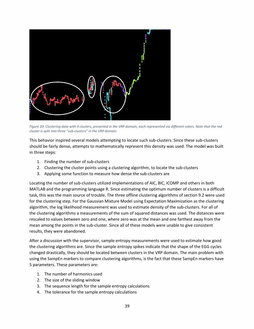
39
Figure 20: Clustering data with 4 clusters, presented in the VRP domain, each represented via different colors. Note that the red cluster is split into three ”sub-clusters” in the VRP domain.
This behavior inspired several models attempting to locate such sub-clusters. Since these sub-clusters
should be fairly dense, attempts to mathematically represent this density was used. The model was built
in three steps:
1. Finding the number of sub-clusters
2. Clustering the cluster points using a clustering algorithm, to locate the sub-clusters
3. Applying some function to measure how dense the sub-clusters are
Locating the number of sub-clusters utilized implementations of AIC, BIC, ICOMP and others in both
MATLAB and the programming language R. Since estimating the optimum number of clusters is a difficult
task, this was the main source of trouble. The three offline clustering algorithms of section 9.2 were used
for the clustering step. For the Gaussian Mixture Model using Expectation Maximization as the clustering
algorithm, the log likelihood measurement was used to estimate density of the sub-clusters. For all of
the clustering algorithms a measurements of the sum of squared distances was used. The distances were
rescaled to values between zero and one, where zero was at the mean and one farthest away from the
mean among the points in the sub-cluster. Since all of these models were unable to give consistent
results, they were abandoned.
After a discussion with the supervisor, sample entropy measurements were used to estimate how good
the clustering algorithms are. Since the sample entropy spikes indicate that the shape of the EGG cycles
changed drastically, they should be located between clusters in the VRP domain. The main problem with
using the SampEn markers to compare clustering algorithms, is the fact that these SampEn markers have
5 parameters. These parameters are:
1. The number of harmonics used
2. The size of the sliding window
3. The sequence length for the sample entropy calculations
4. The tolerance for the sample entropy calculations

40
5. The limit for the spikes; if the SampEn measurement goes above this limit, a SampEn marker is
placed
While these SampEn spikes mean that we have at least some abrupt change in the harmonics, we cannot
be sure what caused them. Further, we have parameters for the clustering algorithms. The number of
harmonics to use, and number of clusters to produce, must be determined before the clustering starts.
9.4.2 Results & Analysis Since most of the recordings are fairly short, only a few seconds long, 12 of them were concatenated to
form a longer recording (77 seconds). In those 12 recordings, the subject performs the same upward
glissandi exercise on the vowel /a/, which simplifies the presentation of the results. In these recordings
we expect to see a transition between clusters in the middle of the VRP, since two voice registers were
used (modal and falsetto). Each recording start in the lower left corner of the VRP and transition towards
the top right corner.
Since it is hard to estimate the optimal settings for the comparison, we start off by locating good settings
for our data. There are four different settings that will be considered here:
1. The number of clusters
2. Phase Portrait or Peak Follower for the cycle separation
3. The number of harmonics used to produce the points
4. Fuzziness parameter for Fuzzy C-Means
Once the seemingly best clustering algorithm has been selected, the SampEn markers will be applied
with different limits. Since we need to conserve space in this master thesis, we start out by figuring out
the optimal configuration for Fuzzy C-Means.
The cluster color coding was modified so that the VRPs look as similar as possible, to help with the
comparison. Thus, when reproducing these results you may end up with different cluster colors, but the
underlying data should still be the same. Note that this only changes the presentation of the clustering
results, and not the data.
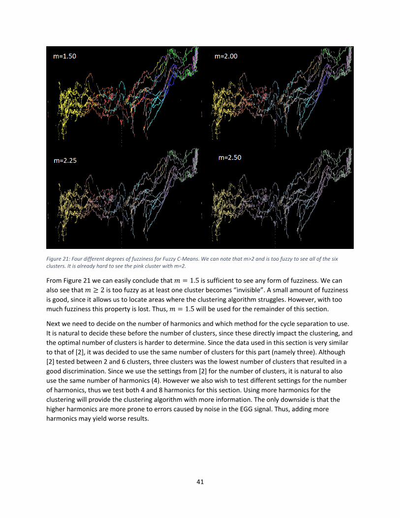
41
Figure 21: Four different degrees of fuzziness for Fuzzy C-Means. We can note that m>2 and is too fuzzy to see all of the six clusters. It is already hard to see the pink cluster with m=2.
From Figure 21 we can easily conclude that 𝑚 = 1.5 is sufficient to see any form of fuzziness. We can
also see that 𝑚 ≥ 2 is too fuzzy as at least one cluster becomes “invisible”. A small amount of fuzziness
is good, since it allows us to locate areas where the clustering algorithm struggles. However, with too
much fuzziness this property is lost. Thus, 𝑚 = 1.5 will be used for the remainder of this section.
Next we need to decide on the number of harmonics and which method for the cycle separation to use.
It is natural to decide these before the number of clusters, since these directly impact the clustering, and
the optimal number of clusters is harder to determine. Since the data used in this section is very similar
to that of [2], it was decided to use the same number of clusters for this part (namely three). Although
[2] tested between 2 and 6 clusters, three clusters was the lowest number of clusters that resulted in a
good discrimination. Since we use the settings from [2] for the number of clusters, it is natural to also
use the same number of harmonics (4). However we also wish to test different settings for the number
of harmonics, thus we test both 4 and 8 harmonics for this section. Using more harmonics for the
clustering will provide the clustering algorithm with more information. The only downside is that the
higher harmonics are more prone to errors caused by noise in the EGG signal. Thus, adding more
harmonics may yield worse results.
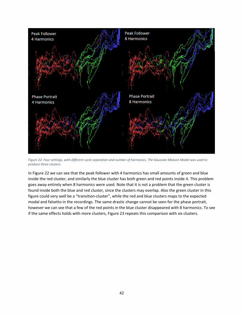
42
Figure 22: Four settings, with different cycle separation and number of harmonics. The Gaussian Mixture Model was used to produce three clusters.
In Figure 22 we can see that the peak follower with 4 harmonics has small amounts of green and blue
inside the red cluster, and similarly the blue cluster has both green and red points inside it. This problem
goes away entirely when 8 harmonics were used. Note that it is not a problem that the green cluster is
found inside both the blue and red cluster, since the clusters may overlap. Also the green cluster in this
figure could very well be a “transition-cluster”, while the red and blue clusters maps to the expected
modal and falsetto in the recordings. The same drastic change cannot be seen for the phase portrait,
however we can see that a few of the red points in the blue cluster disappeared with 8 harmonics. To see
if the same effects holds with more clusters, Figure 23 repeats this comparison with six clusters.
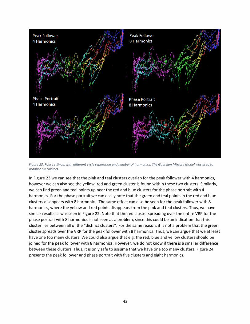
43
Figure 23: Four settings, with different cycle separation and number of harmonics. The Gaussian Mixture Model was used to produce six clusters.
In Figure 23 we can see that the pink and teal clusters overlap for the peak follower with 4 harmonics,
however we can also see the yellow, red and green cluster is found within these two clusters. Similarly,
we can find green and teal points up near the red and blue clusters for the phase portrait with 4
harmonics. For the phase portrait we can easily note that the green and teal points in the red and blue
clusters disappears with 8 harmonics. The same effect can also be seen for the peak follower with 8
harmonics, where the yellow and red points disappears from the pink and teal clusters. Thus, we have
similar results as was seen in Figure 22. Note that the red cluster spreading over the entire VRP for the
phase portrait with 8 harmonics is not seen as a problem, since this could be an indication that this
cluster lies between all of the “distinct clusters”. For the same reason, it is not a problem that the green
cluster spreads over the VRP for the peak follower with 8 harmonics. Thus, we can argue that we at least
have one too many clusters. We could also argue that e.g. the red, blue and yellow clusters should be
joined for the peak follower with 8 harmonics. However, we do not know if there is a smaller difference
between these clusters. Thus, it is only safe to assume that we have one too many clusters. Figure 24
presents the peak follower and phase portrait with five clusters and eight harmonics.
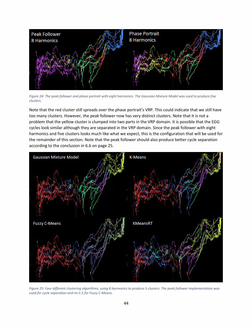
44
Figure 24: The peak follower and phase portrait with eight harmonics. The Gaussian Mixture Model was used to produce five clusters.
Note that the red cluster still spreads over the phase portrait’s VRP. This could indicate that we still have
too many clusters. However, the peak follower now has very distinct clusters. Note that it is not a
problem that the yellow cluster is clumped into two parts in the VRP domain. It is possible that the EGG
cycles look similar although they are separated in the VRP domain. Since the peak follower with eight
harmonics and five clusters looks much like what we expect, this is the configuration that will be used for
the remainder of this section. Note that the peak follower should also produce better cycle separation
according to the conclusion in 6.6 on page 25.
Figure 25: Four different clustering algorithms, using 8 harmonics to produce 5 clusters. The peak follower implementation was used for cycle separation and m=1.5 for Fuzzy C-Means.
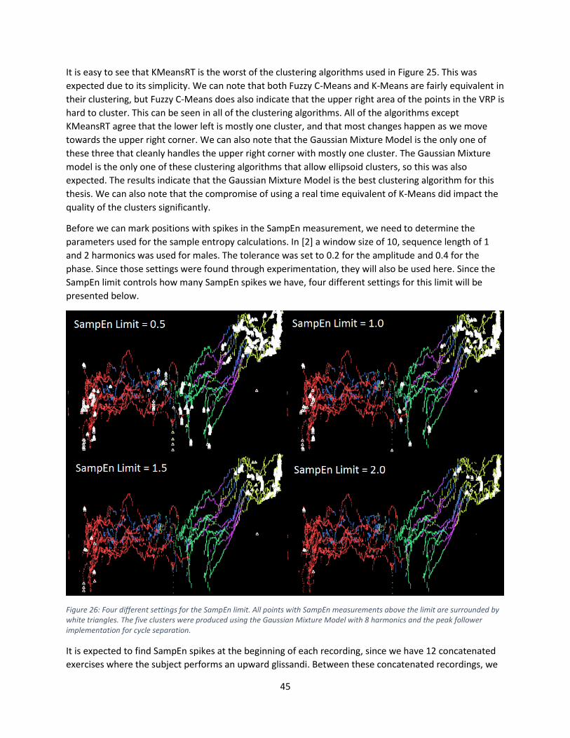
45
It is easy to see that KMeansRT is the worst of the clustering algorithms used in Figure 25. This was
expected due to its simplicity. We can note that both Fuzzy C-Means and K-Means are fairly equivalent in
their clustering, but Fuzzy C-Means does also indicate that the upper right area of the points in the VRP is
hard to cluster. This can be seen in all of the clustering algorithms. All of the algorithms except
KMeansRT agree that the lower left is mostly one cluster, and that most changes happen as we move
towards the upper right corner. We can also note that the Gaussian Mixture Model is the only one of
these three that cleanly handles the upper right corner with mostly one cluster. The Gaussian Mixture
model is the only one of these clustering algorithms that allow ellipsoid clusters, so this was also
expected. The results indicate that the Gaussian Mixture Model is the best clustering algorithm for this
thesis. We can also note that the compromise of using a real time equivalent of K-Means did impact the
quality of the clusters significantly.
Before we can mark positions with spikes in the SampEn measurement, we need to determine the
parameters used for the sample entropy calculations. In [2] a window size of 10, sequence length of 1
and 2 harmonics was used for males. The tolerance was set to 0.2 for the amplitude and 0.4 for the
phase. Since those settings were found through experimentation, they will also be used here. Since the
SampEn limit controls how many SampEn spikes we have, four different settings for this limit will be
presented below.
Figure 26: Four different settings for the SampEn limit. All points with SampEn measurements above the limit are surrounded by white triangles. The five clusters were produced using the Gaussian Mixture Model with 8 harmonics and the peak follower implementation for cycle separation.
It is expected to find SampEn spikes at the beginning of each recording, since we have 12 concatenated
exercises where the subject performs an upward glissandi. Between these concatenated recordings, we
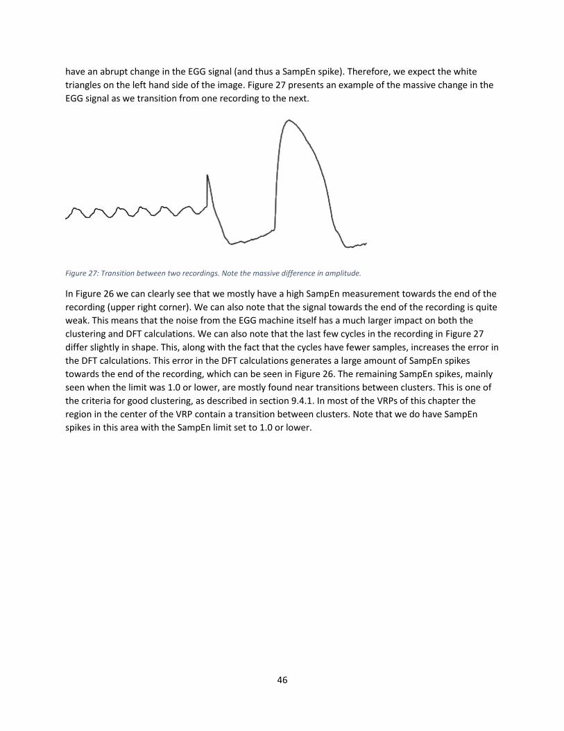
46
have an abrupt change in the EGG signal (and thus a SampEn spike). Therefore, we expect the white
triangles on the left hand side of the image. Figure 27 presents an example of the massive change in the
EGG signal as we transition from one recording to the next.
Figure 27: Transition between two recordings. Note the massive difference in amplitude.
In Figure 26 we can clearly see that we mostly have a high SampEn measurement towards the end of the
recording (upper right corner). We can also note that the signal towards the end of the recording is quite
weak. This means that the noise from the EGG machine itself has a much larger impact on both the
clustering and DFT calculations. We can also note that the last few cycles in the recording in Figure 27
differ slightly in shape. This, along with the fact that the cycles have fewer samples, increases the error in
the DFT calculations. This error in the DFT calculations generates a large amount of SampEn spikes
towards the end of the recording, which can be seen in Figure 26. The remaining SampEn spikes, mainly
seen when the limit was 1.0 or lower, are mostly found near transitions between clusters. This is one of
the criteria for good clustering, as described in section 9.4.1. In most of the VRPs of this chapter the
region in the center of the VRP contain a transition between clusters. Note that we do have SampEn
spikes in this area with the SampEn limit set to 1.0 or lower.

47
10 Graphical User Interface The project heavily relies on presenting information to the user in real time, as the user is vocalizing.
Thus, a brief overview of the different components in the graphical user interface is presented in this
chapter.
10.1 Overview
Figure 28: An overview of the graphical user interface. There are seven main areas of the window, explained in detail below.
The graphical user interface (GUI) consists of:
1. General settings
2. SampEn scope with settings
3. Moving EGG
4. Voice Range Profile with settings
5. Clustering settings
6. Components of the cluster means
7. Cluster counts and the average cluster cycle
The general settings contain settings for input, output and general processing, such as the cycle
separation algorithm. Below these settings we can find all of the information that is presented to the
user. First and foremost, we have the Voice Range Profile (VRP) with its settings on the right hand side.
As explained in the introduction to this thesis, a VRP can use colors to encode different types of
information, such as density, clarity, crest factor, etc. Since the size of the VRP matters, only one of these
types of data can be presented at a time in the VRP plot. There is also an overlay indicating where voice
register transition locations (SampEn spikes) were found. These spikes are indicated as arrows that gives
2
4
6 7
1
3
5

48
the user an indication how the frequency or amplitude of the voice changed as the SampEn spike was
produced. This plot has 200x200 cells for the color data, and 100x100 cells for the SampEn arrows.
The SampEn measurement contains eight different settings, since the settings for the sample entropy
calculations may differ between phase and amplitude data. The settings for the harmonics simply means
that the Fourier Descriptors (FDs) produced by the first n harmonics are used for the sample entropy
calculations. In the VRP view we also have a ninth setting, namely the SampEn limit, which is used to
indicate when a spike should produce a SampEn arrow. Since the SampEn scope is less important, it
shares its space with the moving EGG, which is explained in detail in section 10.2.
The settings for the clustering algorithm can be found right below the SampEn scope, and mostly consists
of flags. These flags can be used to continue learning with previously learned data. They can also be used
to reset the counts for KMeansRT, which has the effect of “forgetting” the old data. This data can also be
saved to and loaded from files. The data is then presented in two parts. The first part (6) shows the
components of the cluster means. As explained in section 2, the points used for the clustering algorithm
are formed by concatenating the differences between the FDs of the fundamental and those of the
harmonics. Thus, with four harmonics, we have three “delta-FDs”, each with its phase and amplitude
component. Using this data, we plot digits for each component, the position indicating its phase and
amplitude. This is repeated for each cluster, unless the slider is used to limit the view to present the
components of one cluster only. The second part (7) has two separate views, the cluster counts and the
average cluster cycle. An average cycle for each cluster can be used to fine tune the parameters for the
clustering algorithm, and is explained in detail in section 10.3. The cluster counts are used internally by
KMeansRT and presents the current distribution of points among the clusters.
10.2 Moving EGG The Moving EGG can be seen as a type of oscilloscope that stores n consecutive cycles for preview [29].
These cycles are presented overlapping each other, where older cycles fade into the background. This
gives the user a good indication of how the cycle changes its shape over time. Such information is
important, since the information that is presented is based on the shape of the EGG cycles. Thus, if the
shape abruptly changes, we expect a SampEn spike and a change of cluster in the VRP. We can also
notice problems with the cycle separation using this tool. If the cycle separation produces changing
placements (see section 6.3), we can notice this immediately, since the moving EGG will appear to
“shake” violently from side to side. Similarly, faulty or missing cycles can be detected, since at least one
cycle is completely different when compared to its neighboring cycles, which is easy to detect in the
moving EGG. Note that it is not guaranteed to pick up these errors in the moving EGG, since the user may
produce several thousands of EGG cycles per second, while we only update the moving EGG 24 times per
second.
Since a small number of samples (< 100) is enough to represent the shape of the signal accurately, and
10-20 consecutive cycles to track easily the changes in real time, transferring this information over to the
client is quite cheap. With 80 samples per cycle and 20 cycles, all this information can fit into a single
/b_getn request. Thus, all of the operations on the buffer should be performed on the server for
performance reasons. Since the buffer must be of a fixed size, we must resample each cycle to a fixed
number of samples. This resampling can sadly not be dealt with like the DFT calculations. For example, if
we resample each cycle into 80 samples and attempt to spread these calculations out over the following
control cycles, we would run into problems when the incoming cycles are shorter than 80 samples. We
49
can of course still spread out the calculations, but it makes the UGen more complex internally, without
gaining much in terms of efficiency. The buffer data still requires us to rotate the data, to guarantee that
it is available in the “drawing order”.
Since we have such a small amount of data, the rotation, normalization and resampling is quite cheap.
Therefore, a decision was made to simply do all of these when the full cycle has ended. This choice
simplifies the design, and avoids delay at a fairly small cost. It does however produce very spiky CPU
usage.
10.3 Average Cycle per Cluster Since the method described in section 2 attempts to cluster based on the shape of the cluster cycle, we
expect that an average cycle should exist. As explained earlier, the average cycle per cluster can be used
to tune the parameters for the number of harmonics and number of clusters. If too few harmonics are
used, or too many clusters are generated, we can detect very similar average cycles for several clusters.
By increasing the number of harmonics, or decreasing the number of clusters, we can see what
generated the error. Similarly, if we generate too few clusters, we can use the combination of the
average cycle for the cluster and the moving EGG to detect whether seemingly different cycles end up in
the same cluster. The average cycle per cluster may also prove an efficient tool to compare clustering
algorithms in future studies.
For the average cycle per cluster, two options were considered. Since we already have the DFT output
ready on the server, it is quite natural to use it to reconstruct the average cycles. The reconstruction of
the average cycle per cluster can be done by averaging together the complex numbers that generated
the points in the cluster, and using the inverse DFT to reconstruct the shape. However, this means that
the number of harmonics we use directly influences the number of points in the reconstructed signal.
Since we currently use less than 20 harmonics, we can only reconstruct the signal with up to 20 points.
This resolution is really poor. Nevertheless, this is the resolution that the clustering is done at, so it might
still be a good approach.
A completely different approach involves generating the average cycle from the cycle samples
themselves. This approach can better utilize the full resolution of the cycles, and may provide a closer
approximation of the average cycle for each cluster.
The second approach was chosen for this project for several reasons, of which the resolution problem is
the main point. Further the second approach is more versatile, since the averaging can be done in many
different ways.
Through experimentation it was found that roughly 80 samples is enough for the cycle to appear smooth
when presented. Hence the implementation of the average cycle is performed via resampling each cycle
into exactly 80 samples. Since the shape of the cycle is of interest we start off by normalizing these 80
samples before merging the results for the cluster.
Rather than using average for the cycles, it was decided to use smoothing instead. This allows us to
change the smooth factor, in the same way as KMeansRT, depending on the number of points in the
cluster, or depending on the total number of points. This should give a similar result as the average
would. The implementation uses a smooth factor that is altered depending on the number of points in
the cluster in the same way as KMeansRT (see section 9.2.1 on page 33). This has the effect of letting the
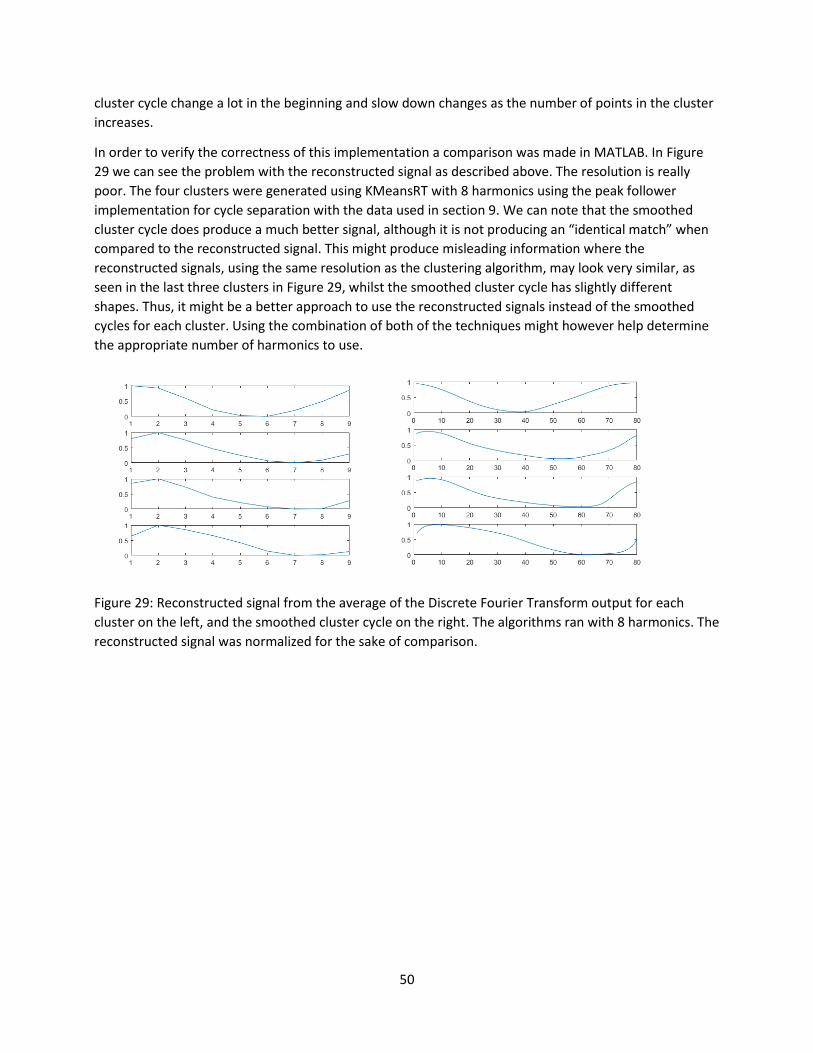
50
cluster cycle change a lot in the beginning and slow down changes as the number of points in the cluster
increases.
In order to verify the correctness of this implementation a comparison was made in MATLAB. In Figure
29 we can see the problem with the reconstructed signal as described above. The resolution is really
poor. The four clusters were generated using KMeansRT with 8 harmonics using the peak follower
implementation for cycle separation with the data used in section 9. We can note that the smoothed
cluster cycle does produce a much better signal, although it is not producing an “identical match” when
compared to the reconstructed signal. This might produce misleading information where the
reconstructed signals, using the same resolution as the clustering algorithm, may look very similar, as
seen in the last three clusters in Figure 29, whilst the smoothed cluster cycle has slightly different
shapes. Thus, it might be a better approach to use the reconstructed signals instead of the smoothed
cycles for each cluster. Using the combination of both of the techniques might however help determine
the appropriate number of harmonics to use.
Figure 29: Reconstructed signal from the average of the Discrete Fourier Transform output for each
cluster on the left, and the smoothed cluster cycle on the right. The algorithms ran with 8 harmonics. The
reconstructed signal was normalized for the sake of comparison.

51
11 Conclusion & Future Work Since there are many different parts of this thesis, the conclusions and future work in this section are
presented for each part separately, in the same order as in the sections of the thesis.
The data transfer was handled with a limited set of tools available in SC version 3.6.6. Writing the results
to disk is solely handled on the server, and works well, since full freedom is given via the plugins. Plugins
are however not available for the client as described in section 4.2. Thus, the client is currently the
bottleneck for the data transfer. This can be improved by modifying the client by adding new primitives.
Whether such a solution will generate extra work in future releases of SC is uncertain. However, there
are many improvements that are possible if the client is modified. First and foremost, the solution in
section 5.1.3 could become completely obsolete, since plugins on the client can utilize the shared
memory interface. This will however only work for local and internal servers. However, such a limitation
may already exist in the current implementation, due to the sheer amount of data that is transferred.
Further, the SC language is a big drawback for the graphics in SC, while this problem can be avoided via
specialized primitives. Using the combination of the shared memory interface and special primitives for
the graphics is exactly how the Stethoscope implementation works in SC version 3.6.6. Note that this is
one of the few SC features that present information from the server, on the client, in real time.
Thus, it is possible to use SC for this project, but it may require special primitives on the client to work
well. The algorithm is however unquestionably capable of running in real time, since the bottleneck is
data transfer and presentation.
The cycle separation may be improved via preprocessing and placing some more focus on the
parameters and implementations of the algorithms. Most focus should be placed on the phase portrait
algorithm, since it offers much potential to work well.
The sample entropy calculations and DFT calculations are already optimized, and should not require
much improvement.
We can conclude that the definition of a good clustering algorithm needs more work. Utilizing the
SampEn markers does not work, and will not scale (if a comparison with more data is required). Note
that scaling is important if further studies require many different configurations for the clustering
algorithms. We can however conclude that an offline clustering algorithm does a better job at clustering
than KMeansRT. This might also extend to other online clustering algorithms. Although the Gaussian
Mixture Model did a slightly better job, these results cannot be fully trusted due to the problems with
the definition of good clusters used in this thesis. More focus should however be placed on the
preprocessing steps and cycle separation to reduce the errors in the DFT calculations. Such
improvements should also have a positive effect on the SampEn markers.
Since the method described in section 2 clusters based on the shape of each EGG cycle, using clustering
algorithms for functional data [26] may yield better results. However, finding online equivalents of such
an algorithm may not be possible.
A better approach for the definition of good clustering may be found in the average cycle per cluster
implementation presented in section 10.3. We can easily extract all cycles of each cluster, and get an
estimation of the average shape of the cycles in these clusters. By using a measurement such as the
mean squared error, an automated algorithm could compare the shape of each cycle, to that of the

52
average cycle in the cluster. This should provide an improved comparison between clustering algorithms,
and may also help identify yet unknown problems by locating cycles that clearly do not belong in the
cluster.
The MovingEGG implementation works well, and should not require any more work, but the average
cycle per cluster requires more work to give better estimations. Since the comparison of the two
approaches for the average cycle per cluster in section 10.3 was fairly limited, a future study will be
required. With a good implementation of the average cycle per cluster, it can be used to improve the
clustering step of the method, as described above.
53
References
[1] Peter Pabon, Rob Stallinga, Maria Södersten, Sten Ternström, "Effects on vocal range and voice
quality of Singing Voice Training; the Classically Trained Female Voice," Journal of Voice, vol. 28, no.
1, pp. 36-51, 2014.
[2] Sten Ternström, Andreas Selamtzis, "Analysis of vibratory states in phonation using spectral
features of the electroglottografic signal," Acoustical Society of America, vol. 136, no. 5, pp. 2773-
2783, 2014.
[3] Roubeau B., Castellengo M., Bodin P., Ragot M., "Phonétogramme par registre laryngé," Folia
Phoniatrica et Logopaedica, vol. 56, no. 5, pp. 321-333, 2004.
[4] Louis Heylen, Floris L. Wuyts, Fons Mertens, Marc De Bodt, Jos Pattyn, Christophe Croux, Paul H.
Van de Heyning, "Evaluation of the Vocal Performance of Children Using a Voice Range Profile
Index," Journal of Speech, Language and Hearing Research, vol. 41, no. 2, pp. 232-238, 1998.
[5] Sten Ternström, Peter Pabon, Maria Södersten, "The Voice Range Profile: Its Function, Applications,
Pitfalls and Potential," Acta Acustica united with Acustica, vol. 101, 2015.
[6] Andrés Pérez-López, "GitHub," 17 10 2014. [Online]. Available:
https://github.com/andresperezlopez/rt-spatialization. [Accessed 09 10 2015].
[7] Håkon Knutzen, "GitHub," 03 10 2014. [Online]. Available:
https://github.com/hakonk/SuperCollider-code. [Accessed 09 10 2015].
[8] Fredrik Olofsson, "GitHub," 15 05 2013. [Online]. Available: https://github.com/redFrik/udk04-
Audiovisual_Programming. [Accessed 09 10 2015].
[9] "SuperCollider," [Online]. Available: http://supercollider.github.io/. [Accessed 16 05 2015].
[10] Scott Wilson, David Cottle, Nick Collins, The SuperCollider Book, Massachusetts Institute of
Technology, 2011.
[11] Philip Bergander, "Fourieranalys av EGG-signaler i realtid," KTH Skolan för Teknik och Hälsa ,
Flemingsberg, 2015.
[12] [Online]. Available: http://doc.sccode.org/Help.html. [Accessed 09 08 2015].
[13] James McCartney, "SuperCollider Server Command Reference," 2002. [Online]. Available:
http://doc.sccode.org/Reference/Server-Command-Reference.html. [Accessed 09 08 2015].
[14] Ladislav O. Dolanský, "An Instantaneous Pitch-Period Indicator," The Journal of the Acoustical
Society of America, vol. 27, no. 1, p. 67, 1955.

54
[15] Agner Fog, "Optimizing softwave in C++," Technical University of Denmark, 07 08 2014. [Online].
Available: http://www.agner.org/optimize/optimizing_cpp.pdf. [Accessed 21 11 2015].
[16] Joshua S. Richman , J. Randall Moorman, "Physiological time-series analysis using approximate
entropy and sample entropy," American Journal of Physiology, vol. 278, no. 6, pp. 2039-2049, 2000.
[17] Yu-Hsiang Pan, Yung-Hung Wang, Sheng-Fu Liang, Kuo-Tien Lee, "Fast computation of sample
entropy and approximate entropy in biomedicine," Computer Methods and Programs in
Biomedicine, vol. 104, no. 3, pp. 382-396, 12 2011.
[18] Angie King, "Online k-Means Clustering of Nonstationary Data," Massachusetts Institute of
Technology OpenCourseWare, Massachusetts, 2012.
[19] P. Hore, L.O. Hall, D.B. Goldgof, W. Cheng, "Online Fuzzy C Means," in Fuzzy Information Processing
Society, 2008. NAFIPS 2008. Annual Meeting of the North American, New York City, 2008.
[20] Mingzhou Song, Hongbin Wang, "Highly Efficient Incremental Estimation of Gaussian Mixture
Models for Online Data Stream Clustering," in Proceedings of SPIE Conference on Intelligent
Computing: Theory and Applications III, 2005.
[21] danstowell, "GitHub / sc3-plugins," 27 11 2012. [Online]. Available:
https://github.com/supercollider/sc3-
plugins/blob/master/source/MCLDUGens/MCLDSOMUGens.cpp. [Accessed 16 05 2015].
[22] J.M Peña, J.A Lozano, P. Larrañaga, "An empirical comparison of four initialization methods for the
K-Means algorithm," Pattern Recognition Letters, vol. 20, no. 10, p. 1027–1040, 1999.
[23] E. Forgy, "Cluster Analysis of Multivariate Data: Efficiency versus Interpretability of Classification,"
Biometrics, vol. 21, no. 3, pp. 768-769, 1965.
[24] A. P. Dempster; N. M. Laird; D. B. Rubin, "Maximum Likelihood from Incomplete Data via the EM
Algorithm," Journal of the Royal Statistical Society, vol. 39, no. 1, pp. 1-38, 1977.
[25] James C. Bezdek, Pattern Recognition with Fuzzy Objective Function Algorithms, New York: Plenum
Press, 1981.
[26] Elizabeth Ann Maharaja, Pierpaolo D’Ursob, "Fuzzy clustering of time series in the frequency
domain," Information Sciences, vol. 181, no. 7, pp. 1187-1211, 2011.
[27] Gilles Celeux, Gilda Soromenho, "An Entropy Criterion for Assessing the Number of Clusters in a
Mixture Model," Journal of Classification, vol. 13, no. 2, pp. 195-212, 1996.
[28] Robert Tibshirani, Guenther Walther, Trevor Hastie, "Estimating the number of clusters in a data
set via the gap statistic," Journal of the Royal Statistical Society, Series B, vol. 63, no. 2, pp. 411-423,
2001.

55
[29] Christian Herbst, "MovingEGG," 2004. [Online]. Available:
http://homepage.univie.ac.at/christian.herbst//movingEgg/about.html. [Accessed 14 10 2015].

56
Appendix A: Rates In the current version (2015-09-15) there are 8 types of outputs. The first output is simply echoing or
playing back the recording. The last 7 are output files explained below. The files are written in one of two
rates:
"Audio Rate" - meaning the same rate as the input
"Good Cycle Rate" - one frame from each good cycle; which means the output has a connection
to the cycle rather than the EGG signal itself.
For more information on how these two rates are connected, see "Connection Between Rates via Gates"
below.
The reason behind storing the information in two different rates is hard drive space. We could in theory
write all the data at audio rate, however this is inefficient since it requires us to repeat the information
connected to cycles for the entire following cycle. This is very inefficient. Another reason behind this
choice, is because we are discarding cycles, which complicates things even more. The final reason is that
we can store the information required to connect the two rates with less bits spent on samples. In this
case we use 16 bit integers to store the audio rate data and 32 bit floating point values to store the
"Good Cycle Rate" data.
Log
With n harmonics we have the following output as an AIFF file with floats representing samples. These
files have "_Log.aiff" as a postfix.
Channel # Content
0 The estimated frequency when the EGG cycle started. Note that this measurement is not scaled.
1 The estimated amplitude when the EGG cycle started. Note that this measurement is not scaled.
2 The clarity measurement when the EGG cycle started. Note that this measurement is not scaled.
3 The crest measurement when the EGG cycle started. Note that this measurement is not scaled.
4 The cluster number of this cycle. Note that this measurement is not scaled.
5 The SampEn measurement for this cycle. Note that this measurement is not scaled.
[6,6+n) The amplitudes in Bels of each of the n harmonics produced.
[6+n,6+2n) The phases in radians in the range (-pi, pi] for each of the n harmonics produced.

57
Recording
This file contains the recording with the following output as a WAV file with 16 bit integers for the
samples. These files have "_Voice_EGG.wav" as a postfix.
Channel # Content
0 The raw Audio input signal.
1 The raw EGG input signal.
Cycle Detection
This file contains the following output as a WAV file with 16 bit integers for the samples. These files have
"_CycleDetection.wav" as a postfix.
Channel # Content
0 The raw EGG input signal.
1 The gate signal used to separate the EGG signal into cycles. This signal is one whenever a new cycle begins.
Points
With n harmonics we have the following output as an AIFF file with floats representing samples. These
files have "_Points.aiff" as a postfix.
Channel # Content
[0,n) The delta amplitude measurements. This is simply the difference between the amplitude of the fundamental frequency and the 2nd, 3rd etc harmonic.
[n,2n) The delta phase measurements. This is simply the difference between the phase of the fundamental frequency and the 2nd, 3rd etc harmonic. Thus, its range is (-2pi, 2pi).
SampEn
This file is an AIFF file with floats representing the samples. These files have "_SampEn.aiff" as a postfix.
Channel # Content
0 The SampEn measurement. Note that this measurement is not scaled.
58
Frequency & Amplitude
This file does not have any on/off button connected to it, but is always written when either the SampEn
measurement is written, or the points are written. The reason being that you often want these together.
The file is an AIFF file with floats as samples. These files have "_FreqAmp.aiff" as a postfix.
Channel # Content
0 The estimated frequency when the EGG cycle started. Note that this measurement is not scaled.
1 The estimated amplitude when the EGG cycle started. Note that this measurement is not scaled.
Connection between Rates via Gates
While it might seem strange to split the information into several files, it is not hard to combine the
information. If the files are written at the same rate - there is no problem; the problems arise when the
files are written in different rates. There is a final special output file - which is written if any "Good Cycle
Rate" files are written, which holds the information required to connect a "Good Cycle" to its exact
position on the EGG signal.
It accomplishes this task via three gates. The cycle gate holds the cycle separation information. This is the
exact same signal written into channel 1 of the CycleDetection file. The delayed cycle gate holds the
same information as the first gate in a way. For each spike (1) in the cycle gate, the delayed cycle gate
will also have a spike, but delayed by an unknown amount. There is one exception, which can be seen in
Figure 30, namely at the end of the recording. This problem arises since the DFT output didn't have
enough time on the server to be calculated, hence there is no matching output for this cycle, and
therefore it can be seen as a clipped cycle. Thus, the delayed cycle gate tells us when the DFT plugin has
computed the results for that cycle, or when it was forced to skip the cycle (due to its length). The
filtered DFT gate tells us which cycles were removed from consideration due to other aspects, such as
poor clarity. This gate will only have spikes where the delayed cycle gate has spikes. If the delayed cycle

59
gate has a spike where the filtered DFT gate does not, it means that the cycle the spike represented was
discarded for some reason.
Figure 30: The three gates. Note that we have one too short cycle, one discarded cycle and one clipped cycle.
This gate file contains the following output as a WAV file with 16 bit integers for the samples. These files
have "_Gates.wav" as a postfix.
Channel # Content
0 The raw EGG signal.
1 The conditioned EGG signal (this is the signal used in the DFT calculations)
2 The Cycle Gate.
3 The Delayed Cycle Gate.
4 The Filtered DFT Gate.
MATLAB Gate Example
The example in this section will grab 3 random good and discarded cycles and present these in plots. For
every good cycle there is a matching entry in all the “good cycle rate” files.
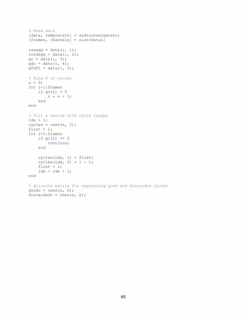
60
% Read data [data, samplerate] = audioread(gates); [frames, channels] = size(data);
rawegg = data(:, 1); condegg = data(:, 2); gc = data(:, 3); gdc = data(:, 4); gfdft = data(:, 5);
% Find # of cycles n = 0; for i=1:frames if gc(i) > 0 n = n + 1; end end
% Fill a matrix with cycle ranges idx = 1; cycles = ones(n, 2); first = 1; for i=1:frames if gc(i) <= 0 continue; end
cycles(idx, 1) = first; cycles(idx, 2) = i - 1; first = i; idx = idx + 1; end
% Allocate matrix for separating good and discarded cycles goodc = ones(n, 2); discardedc = ones(n, 2);
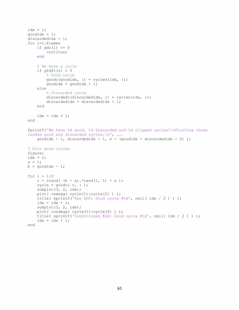
61
idx = 1; goodidx = 1; discardedidx = 1; for i=1:frames if gdc(i) <= 0 continue; end
% We have a cycle if gfdft(i) > 0 % Good cycle goodc(goodidx, :) = cycles(idx, :); goodidx = goodidx + 1; else % Discarded cycle discardedc(discardedidx, :) = cycles(idx, :); discardedidx = discardedidx + 1; end
idx = idx + 1; end
fprintf('We have %d good, %d discarded and %d clipped cycles!\nPlotting three
random good and discarded cycles.\n', ... goodidx - 1, discardedidx - 1, n - (goodidx + discardedidx - 2) );
% Plot good cycles figure; idx = 1; a = 1; b = goodidx - 1;
for i = 1:3 r = round( (b - a).*rand(1, 1) + a ); cycle = goodc( r, : ); subplot(3, 2, idx); plot( rawegg( cycle(1):cycle(2) ) ); title( sprintf('Raw EGG: Good cycle #%d', ceil( idx / 2 ) ) ); idx = idx + 1; subplot(3, 2, idx); plot( condegg( cycle(1):cycle(2) ) ); title( sprintf('Conditioned EGG: Good cycle #%d', ceil( idx / 2 ) ) ); idx = idx + 1; end
62
% Plot discarded cycles figure; idx = 1; a = 1; b = discardedidx - 1;
for i = 1:3 r = round( (b - a).*rand(1, 1) + a ); cycle = discardedc( r, : ); subplot(3, 2, idx); plot( rawegg( cycle(1):cycle(2) ) ); title( sprintf('Raw EGG: Discarded cycle #%d', ceil( idx / 2 ) ) ); idx = idx + 1; subplot(3, 2, idx); plot( condegg( cycle(1):cycle(2) ) ); title( sprintf('Conditioned EGG: Discarded cycle #%d', ceil( idx / 2 ) )
); idx = idx + 1; end
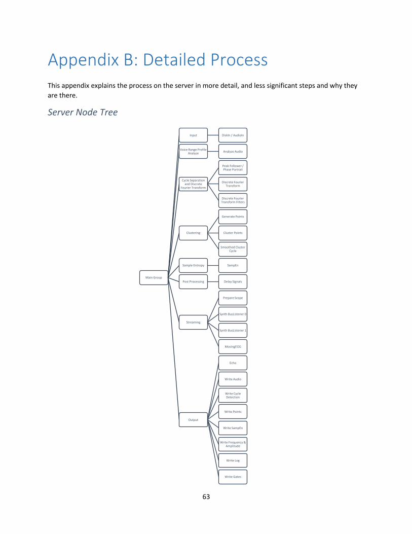
63
Appendix B: Detailed Process This appendix explains the process on the server in more detail, and less significant steps and why they
are there.
Server Node Tree
Main Group
Input DiskIn / AudioIn
Voice Range Profile Analyze
Analyze Audio
Cycle Separation and Discrete
Fourier Transform
Peak Follower / Phase Portrait
Discrete Fourier Transform
Discrete Fourier Transform Filters
Clustering
Generate Points
Cluster Points
Smoothed Cluster Cycle
Sample Entropy SampEn
Post Processing Delay Signals
Streaming
Prepare Scope
Synth BusListener 0
Synth BusListener 1
MovingEGG
Output
Echo
Write Audio
Write Cycle Detection
Write Points
Write SampEn
Write Frequency & Amplitude
Write Log
Write Gates

64
All of the Synths are housed inside their own groups indicating the major steps in the overall process.
These groups are however kept inside the main group, the reason behind this is DiskIn. DiskIn knows
when we have reached the end of the recording. In order to guarantee that the rest of the tree does not
continue processing after DiskIn has stopped, it will pause the main group. A notification is also sent to
the client, so that it can update its user interface.
The “analyze audio” step has not been covered earlier, but involves grabbing the frequency and
amplitude estimations for the Voice Range Profile, i.e. the position in the plot. It also estimates the crest
factor and clarity. This step will not be covered here, since it merely depends on built in UGens.
The cycle separation and Discrete Fourier Transform (DFT) has been thoroughly covered in section 6 and
7 and will not be covered here. In order to filter out the DFT output from bad cycles, we simply place a
filter on the output gate from the DFT synth. This produces a new gate, where the bad cycles have been
discarded. This technique is presented in Figure 30 on page 59.
Section 9 of this master thesis covers all that has to do with clustering, and section 10 explains the tools.
We can also see the server side part of the BusListener implementation thoroughly explained in section
5.1.3. The “prepare scope” step simply generates time stamps that are used to present the SampEn
scope. The contents of the files written in the Output group are all covered in Appendix A, and how these
are written in section 5.2. Thus, none of these will be covered here.
We can see one step unaccounted for, namely the delay step. This step is necessary since we are working
with four different rates on the server:
1. Audio Rate
2. Cycle Rate
3. Delayed Cycle Rate
4. Filtered DFT Rate
We get input at audio rate, this is then split into cycles, where the data associated with these cycles are
stored at cycle rate. However, as explained in section 7 the DFT calculations are spread out in time. Thus,
we need to delay the data associated with these cycles. This is the job done in the delay step, which
writes output at the delayed cycle rate.

www.kth.se


![AA. VV. - The SuperCollider Book [Beginner's Tutorial]](https://img.pdfslide.us/doc/110x75/55cf97ff550346d03394ebd4/aa-vv-the-supercollider-book-beginners-tutorial.jpg)