Embed Size (px)
Citation preview
RealOptions Signaling Games withApplications to Corporate Finance
Steven R. GrenadierStanford University
Andrey MalenkoMassachusetts Institute of Technology
We study games in which the decision to exercise an option is a signal of private informa-tion to outsiders, whose beliefs affect the utility of the decision-maker. Signaling incen-tives distort the timing of exercise, and the direction of distortion depends on whether thedecision-maker’s utility increases or decreases in outsiders’ belief about the payoff fromexercise. In the former case, signaling incentives erode the value of the option to wait andspeed up option exercise, while in the latter case option exercise is delayed. We demon-strate the model’s implications through four corporate finance settings: investment undermanagerial myopia, venture capital grandstanding, investment under cash flow diversion,and product market competition. (JELG31, D82)
The real options approach to investment and other corporate financedecisions has become an increasingly important area of research in financialeconomics. The main underlying concept is that an investment opportunityis valuable not only because of associated cash flows but also because thedecision to invest can be postponed. As a result, when making the investmentdecision, one must take into account both the direct costs of investment and theindirect costs of foregoing the option to invest in the future. The applicationsof the real options framework have become quite broad.1
We thank the anonymous referee, Anat Admati, Felipe Aguerrevere, Geert Bekaert, Nina Boyarchenko, CeciliaBustamante, Nadya Malenko, Ilya Strebulaev, Pietro Veronesi (the editor), Neng Wang, Jeffrey Zwiebel, seminarparticipants at Stanford University, and participants at the 2010 Western Finance Association Annual Meetingin Victoria, BC; the 2010 UBC Winter Finance Conference; and the 9th Trans-Atlantic Doctoral Conferenceat LBS for their helpful comments. Send correspondence to Steven R. Grenadier, Graduate School of Business,Stanford University, 655 Knight Way, Stanford, CA, 94305. E-mail: [email protected]. Andrey Malenko: MITSloan School of Management, 100 Main Street, E62-619, Cambridge, MA, 02142. E-mail: [email protected].
1 The early literature, started byBrennan and Schwartz(1985) andMcDonald and Siegel(1986), is wellsummarized inDixit and Pindyck (1994). Recently the real options framework has been extended to in-corporate competition among several option holders (e.g.,Grenadier 2002;Lambrecht and Perraudin 2003;Novy-Marx 2007) and agency conflicts (Grenadier and Wang 2005). Real options models have been ap-plied to study specific industries such as real estate (Titman 1985; Williams 1991) and natural resources(Brennan and Schwartz 1985) and other corporate decisions such as defaults (e.g.,Leland 1994) andmergers (Lambrecht 2004;Morellec and Zhdanov 2005;Hackbarth and Morellec 2008; Hackbarth andMiao 2011). SeeLeslie and Michaels(1997) for a discussion of how practitioners use real options ideas.
c© The Author 2011. Published by Oxford University Press on behalf of The Society for Financial Studies.All rights reserved. For Permissions, please e-mail: [email protected]:10.1093/rfs/hhr071 Advance Access publication August 3, 2011
at MIT
Libraries on N
ovember 12, 2011
http://rfs.oxfordjournals.org/D
ownloaded from
TheReview of Financial Studies / v 24 n 12 2011
One aspect that is typically ignored in standard models is that most realoptions exercise decisions are made under asymmetric information: Thedecision-maker is better informed about the value of the option than outsiders.Given the importance of asymmetric information in corporate finance, it is use-ful to understand how it affects real options exercise decisions.2 In this article,we explore this issue by incorporating information asymmetry into real optionsmodeling. We consider a setting that is flexible enough to handle a varietyof real-world examples, characterize the effects of asymmetric information,and then illustrate the model using four specific applications: investment undermanagerial myopia, venture capital grandstanding, investment under cash flowdiversion by the manager, and product market entry decisions by two asym-metrically informed firms.
In the presence of asymmetric information, the exercise strategy of a realoption is an important information transmission mechanism. Outsiders learninformation about the decision-maker from observing the exercise (or lack ofexercise) of the option, and thereby change their assessment of the decision-maker. In turn, because the decision-maker is aware of this information trans-mission effect, the option exercise strategy is shaped to take advantage of it.To provide further motivation for the study, consider two examples of optionsexercise decisions, where asymmetric information and signaling are likely tobe especially important.
Example 1. Delegated investment decisions in corporations.In mostmodern corporations, the owners of the firm delegate investment decisions tothe manager. There is substantial asymmetric information: The manager is typ-ically much better informed about the underlying cash flows of the investmentproject than the shareholders. In this context, the manager’s decision when toinvest transmits information about the project’s net present value (NPV). Whilein some agency settings the manager may want to signal higher project valuesto boost her future compensation, in other agency settings the manager maywant to signal a lower project NPV to divert more value for her own privateconsumption. In either setting, however, the manager will take this informationtransmission effect into account when deciding when to invest.
Example 2. Exit decisions in the venture capital industry.In the ven-ture capital (VC) industry, there is substantial asymmetric information aboutthe value of the fund’s portfolio companies, since the VC firm that manages thefund has much better information about the fund’s portfolio companies thanthe fund’s outside investors. In this context, the firm’s decision when to sella portfolio company transmits information about its value, and hence impactsoutsiders’ inferences of the firm’s investment skill. Because investor inferencesof the firm’s investment skill impact the firm’s future fund-raising ability, the
2 SeeTirole (2006), Chapter 6, for a discussion of asymmetric information in corporate finance.
3994
at MIT
Libraries on N
ovember 12, 2011
http://rfs.oxfordjournals.org/D
ownloaded from
RealOptions Signaling Games with Applications to Corporate Finance
firm will take this information transmission effect into account when decidingwhen to sell a portfolio company.
We call such interactions real options signaling games, and study them indetail in this article. We begin our study with a general model of optionsexercise under asymmetric information. Specifically, we consider a decision-maker whose payoff from option exercise comprises two components. The firstcomponent is simply some fraction of the project’s payoff. The second compo-nent, which we call the belief component, depends on outsiders’ assessment ofthe decision-maker’s type. The decision-maker’s type determines the project’sNPV and is the private information of the decision-maker. Our central inter-est is in separating equilibria—equilibria in which the decision-maker revealsher type through the options exercise strategy.3 We characterize a separatingequilibrium of the general model, and prove that under standard regularity con-ditions it exists and is unique. The equilibrium is determined by a differentialequation given by local incentive compatibility.
We show that the implied options exercise behavior differs significantlyfrom traditional real options models. The first-best (symmetric information)exercise threshold is never an equilibrium outcome, except for the most ex-treme type: Because the decision-maker’s utility depends on outsiders’ beliefabout the decision-maker’s type, there is an incentive to deviate from the sym-metric information threshold to mimic a different type and thereby take advan-tage of outsiders’ incorrect belief. While information asymmetry distorts thetiming of options exercise, the direction of the effect is ambiguous and dependson the nature of the interactions between the decision-maker and outsiders.
The first contribution of our article is the characterization of the direction ofdistortion. We show that the direction of distortion depends on a simple and in-tuitive characteristic: the derivative of the decision-maker’s payoff with respectto the belief of outsiders about the decision-maker’s type. If the decision-makerbenefits from outsiders believing that the project’s value is higher than in re-ality, then signaling incentives lead to earlier options exercise than in the caseof symmetric information. In contrast, if the decision-maker benefits from out-siders believing that the project’s value is lower than in reality, then the optionis exercised later than in the case of symmetric information. The intuition un-derlying this result comes from the fact that earlier exercise is a signal of thebetter quality of the project. For example, other things equal, an oil-producingfirm decides to drill an oil well at a lower oil price threshold when it believesthat the quality of the oil well is higher. Because of this, if the decision-makerbenefits from outsiders believing that the project’s quality is higher (lower)than in reality, she has incentive to deviate from the first-best exercise thresh-old by exercising the option marginally earlier (later) and attempting to fool the
3 In fact, as we discuss in Section 2.4, any non-separating equilibrium can be ruled out using the D1 restriction onthe out-of-equilibrium beliefs of outsiders.
3995
at MIT
Libraries on N
ovember 12, 2011
http://rfs.oxfordjournals.org/D
ownloaded from
TheReview of Financial Studies / v 24 n 12 2011
market into believing that the project’s quality is higher (lower) than in reality.In equilibrium, the exercise threshold will be lowered (raised) to the point atwhich the decision-maker’s marginal costs of inefficiently early (late) exer-cise exactly offset her marginal benefits from fooling outsiders. Importantly,outsiders are rational. They are aware that the decision-maker shapes the exer-cise strategy to affect their belief. As a result, in equilibrium outsiders alwayscorrectly infer the private information of the agent. However, even though theprivate information is always revealed in equilibrium, signal-jamming occurs:The exercise thresholds of all types, except for the most extreme type, are dif-ferent from the first-best case and are such that no type has an incentive to fooloutsiders.
The second contribution of our article is illustrating the general model withfour corporate finance applications that put additional structure on the be-lief component of the decision-maker’s payoff: investment under managerialmyopia, venture capital grandstanding, investment under cash flow diversionby the manager, and product market entry decisions by two asymmetricallyinformed firms. The first application we consider is a timing analogue to themyopia model ofStein(1989). We consider a public corporation, in which theinvestment decision is delegated to a manager, who has superior informationabout the project’s NPV. As inStein(1989), the manager is myopic in that shecares not only about the long-term performance of the company but also aboutthe short-term stock price. The timing of investment reveals the manager’sprivate information about the project and thereby affects the stock price. Asa result, the manager invests inefficiently by exercising her investment optiontoo early in an attempt to fool the market into overestimating the project’s NPVand thereby inflating the current stock price.
The second application deals with the VC industry. As discussed inGompers(1996), younger VC firms often take companies public earlier than older VCfirms to establish a reputation and successfully raise capital for new funds.Gompers terms this phenomenon “grandstanding” and suggests that inexpe-rienced VC firms employ early timing of initial public offerings (IPOs) as asignal of their ability to form higher-quality portfolios. We formalize this ideain a two-stage model of VC investment. An inexperienced VC firm investslimited partners’ money in the first round and then decides when to take itsportfolio company public. Limited partners update their estimate of the gen-eral partner’s investment-picking ability by observing when the decision totake the portfolio company public is made and use this estimate when decidinghow much to invest in the second round. Because the amount of second-roundfinancing is positively related to the limited partners’ estimate of the generalpartner’s ability, the general partner has an incentive to fool the limited part-ners into believing that her ability is higher. Since an earlier IPO is a signal ofbetter quality of the inexperienced general partner, signaling incentives lead toearlier than optimal exit timing of inexperienced general partners, consistentwith the grandstanding phenomenon ofGompers(1996).
3996
at MIT
Libraries on N
ovember 12, 2011
http://rfs.oxfordjournals.org/D
ownloaded from
RealOptions Signaling Games with Applications to Corporate Finance
Theother two applications belong to the case of the decision-maker benefit-ing more when outsiders believe that the project’s NPV is lower than in reality,and thus imply an inefficiently delayed options exercise. Similar to the firstapplication, the third application studies a delegated investment decision in acorporation. However, unlike the second application, the nature of the agencyconflict is different. Specifically, we consider a setting in which a managercan divert a portion of the project’s cash flows for private consumption, whichmakes the problem a timing analogue of the literature on agency, asymmet-ric information, and capital budgeting (e.g.,Harris, Kriebel, and Raviv 1982;Stulz 1990; Bernardo, Cai, and Luo 2001). In this application, private infor-mation gives the manager an incentive to delay investment so that outside in-vestors underestimate the true NPV of the project, which allows the managerto divert more without being caught. This creates incentives to fool outsideinvestors by investing as if the project was worse than in reality and therebyleads to later investment than in the case of symmetric information. In equilib-rium, outside investors correctly infer the NPV of the project, but still signal-jamming occurs: Investment is inefficiently delayed to prevent the managerfrom fooling outside investors.
Finally, the fourth application we consider is sequential entry into a productmarket in the duopoly framework outlined in Chapter 9 ofDixit and Pindyck(1994). The major distinction of our application is that we relax the assumptionthat both firms observe the potential NPV from launching the new product. In-stead, we assume that the two firms are asymmetrically informed: One firmknows the project’s NPV, while the other learns it from observing the in-vestment (or lack of investment) of the better-informed firm. As a result, thebetter-informed firm has an incentive to delay investment to signal that thequality of the project is worse than in reality and thereby delay the entry ofits competitor and enjoy monopoly power for a longer period of time. Thus,the timing of investment is inefficiently delayed. However, the underinformedfirm rationally anticipates the delay of investment by the better-informed firm,so in equilibrium the timing of investment reveals the NPV of the producttruthfully.
Our findings have a number of implications. First, the effect of informa-tion asymmetry on investment timing is far from straightforward. In fact,information asymmetry can both speed up and delay investment, thus leadingto overinvestment and underinvestment, respectively. The direction of distor-tion depends on the nature of the agency conflict between the manager andshareholders. For example, both the first and the third applications deal withcorporate investment under asymmetric information and agency, but have dif-ferent implications for the effect of information asymmetry on investment. Ifthe agency problem is in managerial short-termism, then asymmetric informa-tion leads to earlier investment. In contrast, if the agency problem is in themanager’s ability to divert cash flows for personal consumption, then asym-metric information leads to later investment.
3997
at MIT
Libraries on N
ovember 12, 2011
http://rfs.oxfordjournals.org/D
ownloaded from
TheReview of Financial Studies / v 24 n 12 2011
Second,because the degree of distortion depends on a simple and intuitivemeasure, one can evaluate the qualitative effect of asymmetric information onthe timing of investment even in complicated settings with multiple agencyconflicts of differing natures. Clearly, in the real world, there are many potentialagency conflicts, including managerial short-termism and the ability to divertcash flows among others. One can obtain the resulting effect of asymmetricinformation by looking at the effect on the manager’s payoff of a marginalchange in the belief of outsiders. This characterization can be important forempirical research, as it implies a clear-cut relation between investment, onthe one hand, and the complicated structure of managerial incentives, on theother hand.
Finally, regarding the last application, our findings demonstrate that com-petitive effects on investment can be significantly weakened if the competitorsare asymmetrically informed about the value of the investment opportunity.A substantial literature on real options (e.g.,Williams 1993; Grenadier 2002)argues that the fear of being preempted by a rival erodes the value of theoption to wait and, as a consequence, speeds up investment. However, whenthe competitors are asymmetrically informed about the investment opportu-nity, better-informed firms have incentives to fool the uninformed firms intounderestimating the investment opportunity and delaying their investment. Thebetter-informed firms achieve this by investing later than in the symmetric in-formation case. Thus, signaling incentives imply an additional value of wait-ing, and therefore greater delay in the firms’ investment decisions.
Our article combines the traditional literature on real options with theextensive literature on signaling. It is most closely related to real options mod-els with imperfect information.Grenadier(1999),Lambrecht and Perraudin(2003), andHsu and Lambrecht(2007) study options exercise games with in-formation imperfections, however, with very different equilibrium structuresthan in this article. InGrenadier(1999), each firm has an imperfect privatesignal about the true project value. InLambrecht and Perraudin(2003), eachfirm knows its own investment cost but not the investment cost of the competi-tor. And in Hsu and Lambrecht (2007), an incumbent is uninformed about thechallenger’s investment cost. While these papers study options exercise withinformation imperfections of various forms, the beliefs of outsiders do not en-ter the payoff function of agents. Therefore, the models in these papers arenot examples of real options signaling games: The informed decision-makerhas no incentives to manipulate investment timing so as to alter the belief ofoutsiders.4
4 Our application on cash flow diversion is also related toGrenadier and Wang(2005) andBouvard(2010), whostudy investment timing under asymmetric information between the manager and investors, where the timing ofinvestment can be part of the contract between the parties. The major difference between their models and ourdiversion application is that theirs are screening models, while ours is a signaling model.
3998
at MIT
Libraries on N
ovember 12, 2011
http://rfs.oxfordjournals.org/D
ownloaded from
RealOptions Signaling Games with Applications to Corporate Finance
Notably, Morellec and Schurhoff (2011) and Bustamante (forthcoming) de-velop models that are examples of real options signaling games, and thus canbe thought of in the context of our general model. Specifically, inMorel-lec and Schurhoff (2011), an informed firm, seeking external resources to fi-nance an investment project, can choose both the timing of investment and themeans of financing (debt or equity) of the project. In Bustamante (forthcom-ing), an informed firm can decide on both the timing of investment and whetherto finance its investment project through an IPO or costlier private capital.Bustamante (forthcoming) andMorellec and Schurhoff (2011) find that asym-metric information speeds up investment as the firm attempts to signal betterquality and thereby secure cheaper financing. Our contribution relative to thesepapers is the characterization of the distortion of investment in a general settingof real options signaling games, which allows for a wide range of environmentswhere real options are common, such as public corporations, VC industry,or entrepreneurial firms. First, we show that whether asymmetric informa-tion speeds up or delays investment depends critically on the nature of theinteractions between the decision-maker and outsiders. In fact, as we show inthe applications, signaling incentives can often delay investment, unlike inBustamante (forthcoming) andMorellec and Schurhoff (2011) where signalingincentives always speed up investment because of the specific nature of theinteractions between the manager and outsiders. Second, we characterize theexact conditions when each of the two distortions is in place. This impliesspecific predictions for each particular institutional setting and shows whena distortion induced by one type of agency conflict (e.g., possibility ofcash flow diversion) can be overturned by the presence of another agencyconflict (e.g., managerial short-termism). Finally,Benmelech, Kandel, andVeronesi(2010) consider a dynamic model of investment with asymmetricinformation between the manager and outsiders and show that in thepresence of stock-based compensation, asymmetric information createsincentives to conceal bad news about growth options. Unlike our article,they focus on a specific setting and do not model investment as a realoption.
The remainder of the article is organized as follows. In Section1, we for-mulate the general model of options exercise in a signaling equilibrium andconsider the special case of symmetric information. In Section2, we solve forthe separating equilibrium of the model, prove its existence and uniqueness,and determine when asymmetric information leads to earlier or later optionsexercise. In Section3, we consider two examples of real options signalinggames in which signaling incentives speed up options exercise: investmentin the presence of managerial myopia and VC grandstanding. In Section4,we consider two examples of real options signaling games in which signalingincentives delay option exercise: investment under the opportunity to divertcash flows and strategic entry to the product market. Finally, we conclude inSection5.
3999
at MIT
Libraries on N
ovember 12, 2011
http://rfs.oxfordjournals.org/D
ownloaded from
TheReview of Financial Studies / v 24 n 12 2011
1. Model Setup
In this section, we present a general model of a real options signaling game.Then, as a useful benchmark, we provide the solution to the first-best case ofsymmetric information. For the ease of exposition, we discuss the model as ifthe real option is an option to invest. However, this is without loss of generality.For example, the real option can also be an option to penetrate a new market,make an acquisition, or sell a business.
1.1 The real optionThe firm possesses a real option of the standard form: At any timet , the firmcan spend a costθ > 0 to install an investment project. The project has apresent valueP (t), representing the discounted expected cash flows. Follow-ing the standard real options framework (e.g.,McDonald and Siegel 1986;Dixit and Pindyck 1994), we assume thatP (t) evolves as a geometric Brown-ian motion:
d P (t) = μP (t) dt + σ P (t) d B (t) , (1)
whereσ > 0 andd B (t) is the increment of a standard Brownian motion.All agents in the economy are risk-neutral, with the risk-free rate of interestdenoted byr . To ensure finite values, we assumeμ < r .5 If the firm invests attime t , it gets the value of
P (t)− θ + ε, (2)
whereε is a zero-mean noise term, reflecting the difference between the re-alized value of the project and its expected value upon investment. It reflectsuncertainty over the value of the project at the time of investment, which canstem from random realized cash flows or random installation costs.
The investment decision is made by the agent, who has superior informationabout the NPV of the project. Specifically,P (t) is publicly observable andknown to both the agent and outsiders. In contrast,θ is the private informa-tion of the agent, which we refer to as the agent’s (or project’s) type. Becausethe payoff of the project depends onθ negatively, higher types correspond toworse projects. Outsiders do not have any information aboutθ except for its ex-ante distribution, which is given by the cumulative distribution functionΦ (∙)with positive density functionφ (∙) defined on
[θ, θ
], whereθ > θ > 0.6
Thus,the payoff from investment comprises three components: the publiclyobservable componentP (t), the privately observable componentθ , and the
5 SeeMcDonaldand Siegel(1986) and Chapter 5 ofDixit and Pindyck(1994) for a discussion of this restriction.Instead of risk neutrality, we could assume thatP (t) evolves as (1) under the risk-neutral measure.
6 Theassumption that the privately observable component of the project is the investment cost is without loss ofgenerality. The model can also be formulated when the privately observable componentθ correspondsto part ofthe project’s present value rather than the investment cost (as inGrenadier and Wang 2005) or when it affects thepresent value of the project multiplicatively (as in Bustamante forthcoming andMorellec and Schurhoff 2011).
4000
at MIT
Libraries on N
ovember 12, 2011
http://rfs.oxfordjournals.org/D
ownloaded from
RealOptions Signaling Games with Applications to Corporate Finance
noisetermε. Outsiders will update their belief about the type of the agent byobserving the timing of investment and its proceeds. The noise termε ensuresthat proceeds from investment provide only an imperfect signal of the agent’sprivate information.7
1.2 The agent’s utility from exerciseHaving characterized the project payoff, we move on to the utility that theagent receives from exercise. We assume that the agent’s utility from exer-cise is the sum of two components. The first component is the direct effect ofthe proceeds from the project on the agent’s compensation. This effect can beexplicit, such as through the agent’s stock ownership in the firm, or implicit,such as through future changes in the agent’s compensation. For tractabilityreasons, we abstain from solving the optimal contracting problem, and insteadsimply assume that the agent receives a positive shareα of the total payofffrom the investment project.8 The second component is the indirect effect ofinvestment on the agent’s utility due to its effect on outsiders’ belief about theagent’s type. Intuitively, the timing of investment can reveal information aboutthe agent, such as an ability to generate profitable investment projects. Lettingθ denote outsiders’ inference about the type of the agent after the investment,the agent’s utility from the option exercise is
Agent’s utility from exercise= share of project+ belief component
= α (P (τ )− θ + ε)+ W(θ , θ
). (3)
While standard real options models typically assume that the agent’s utility issolely a function of the option payoff, in this case the agent also cares about thebelief of outsiders, in thatθ explicitly enters into the agent’s payoff function.The form of the utility function is general enough to accommodate a varietyof settings in which a real option is exercised by a better-informed party whocares about the belief of less-informed outsiders.9
Following Mailath(1987), we impose the following regularity conditions on
W(θ , θ
):
7 We introduce the noise term to make the timing of exercise a meaningful signal of the agent’s private information.If ε werealways equal to zero, then outsiders would be able to learn the exact value ofθ from observing therealized value of the project. As a consequence, the timing of exercise would have no information role. Becauseof risk neutrality, as long as there is some noise, its distribution is not important for our results, with the exceptionof the model in Section 4.1, where its distribution impacts the underlying costly state verification model.
8 SeeGrenadierand Wang(2005) andPhilippon and Sannikov(2007) for optimal contracting problems in the realoptions context.
9 Theform of the utility function from exercise in (3) is chosen to keep the model both tractable and sufficientlygeneral. We have also solved the model for an even more general utility function,α (F (P (τ ))− θ + ε) +
W(
P (τ ) , θ , θ). The results are very similar, as long as the utility function satisfies the regularity conditions in
Mailath (1987).
4001
at MIT
Libraries on N
ovember 12, 2011
http://rfs.oxfordjournals.org/D
ownloaded from
TheReview of Financial Studies / v 24 n 12 2011
Assumption1. W(θ , θ
)is C2 on
[θ, θ
]2;
Assumption2. W (θ, θ) < αθ ;
Assumption 3. Wθ
(θ , θ
)never equals zero on
[θ, θ
]2, and so is either
positive or negative;
Assumption 4. W(θ , θ
)is such thatWθ
(θ , θ
)< α ∀
(θ , θ
)∈[θ, θ
]2
andWθ (θ, θ)+ Wθ (θ, θ) < α ∀θ ∈[θ, θ
];
Assumption 5. Agent’s utility from exercise satisfies the single-crossingcondition, defined in Appendix A.
These conditions allow us to establish the existence and uniqueness of theseparating equilibrium derived in the following section. Assumption 1 is astandard smoothness restriction. Assumption 2 states that under perfect infor-mation the effect of the belief component does not exceed the direct effectof θ . This ensures that the exercise decision is non-trivial, because otherwisethe optimal exercise decision would be to invest immediately for any project’spresent valueP (t). Assumption 3 is the belief monotonicity condition, whichrequires the agent’s payoff to be monotone in outsiders’ belief about the agent’stype. This defines two cases to be analyzed. IfWθ < 0, then the agent benefitsif outsiders believe that the project has a lower investment cost. Conversely, ifWθ > 0, then the agent gains from belief of outsiders that the project has ahigher investment cost. Assumption 4 means that the agent is better off from
having a better project:Wθ
(θ , θ
)< α implies that the agent’s utility from
exercise is decreasing inθ for any fixed level of the outsiders’ belief; simi-larly, Wθ (θ, θ) + Wθ (θ, θ) < α implies that the agent’s utility from exerciseis decreasing inθ if both the agent and outsiders knowθ . Finally, Assump-tion 5 ensures that if the agent does not make extra gains by misrepresentingθ slightly, then she cannot make extra gains from a large misrepresentation. Itallows us to find the separating equilibrium by considering only the first-ordercondition.
1.3 Symmetric information benchmarkAs a benchmark, we consider the case in which information is symmetric.Specifically, assume that both the agent and outsiders observeθ .10 Let V∗
(P, θ) denote the value of the investment option to the agent, if the type of theagent isθ and the current level ofP (t) is P. Using standard arguments (e.g.,Dixit and Pindyck 1994), in the range prior to investment,V∗ (P, θ)must solvethe differential equation:
0 =1
2σ 2P2V∗
PP + μPV∗P − r V∗. (4)
10 If neither the agent nor outsiders observeθ , then the model is analogous to the one in this section.
4002
at MIT
Libraries on N
ovember 12, 2011
http://rfs.oxfordjournals.org/D
ownloaded from
RealOptions Signaling Games with Applications to Corporate Finance
Supposethat the agent of typeθ invests the first time whenP (t) crossesthresholdP∗ (θ) from below. Upon investment, the payoff of the agent is spec-ified in (3), implying the boundary condition for the agent’s expected payofffrom exercise:
V∗ (P∗ (θ) , θ)
= α(P∗ (θ)− θ
)+ W (θ, θ) . (5)
Solving (4) subject to boundary condition (5) yields the following option valueto the agent:11
V∗ (P, θ) =
(P
P∗(θ)
)β(α (P∗ (θ)− θ)+ W (θ, θ)) , if P ≤ P∗ (θ) ,
α (P − θ)+ W (θ, θ) , if P > P∗ (θ) ,
(6)
whereβ is the positive root of the fundamental quadratic equation12σ
2β(β − 1)+ μβ − r = 0:
β =1
σ 2
−
(
μ−σ 2
2
)
+
√(μ−
σ 2
2
)2
+ 2rσ 2
> 1. (7)
The investment triggerP∗ (θ) is chosen by the agent so as to maximizeher value:
P∗ (θ) = arg maxP∈R+
{1
Pβ
(α(
P − θ)
+ W (θ, θ))}. (8)
Taking the first-order condition, we conclude thatP∗ (θ) is given by
P∗ (θ) =β
β − 1
(θ −
W (θ, θ)
α
). (9)
In particular, if W (θ, θ) = 0, we get the standard solution (e.g.,Dixit andPindyck 1994):P∗ (θ) = θβ/ ( β − 1). Because the agent’s utility from ex-ercise is decreasing inθ by Assumption 4, the investment thresholdP∗ (θ) isincreasingin θ , which means that the firm invests earlier if the project is better.
The results of the benchmark case can be summarized in Proposition1:
Proposition 1. Suppose thatθ is known both to the agent and to outsiders.Then, the investment threshold of typeθ , P∗ (θ), is given by (9) and is increas-ing in θ .
11 SinceP = 0 is an absorbing barrier,V∗ (P, θ) mustalso satisfy the conditionV∗ (0,θ) = 0.
4003
at MIT
Libraries on N
ovember 12, 2011
http://rfs.oxfordjournals.org/D
ownloaded from
TheReview of Financial Studies / v 24 n 12 2011
2. Analysis
In this section, we provide the solution to the general real options signalinggame under asymmetric information between the agent and outsiders. First, wesolve for the agent’s optimal exercise strategy for a given inference function ofoutsiders. Then, we apply the rational expectations condition that the inferencefunction must be consistent with the agent’s exercise strategy. This gives usthe equilibrium investment threshold. We present a heuristic analysis in thissection and prove that it indeed yields the unique separating equilibrium inProposition 2. Finally, we analyze properties of the equilibrium.
2.1 Optimal exerciseTo solve for the separating equilibrium, consider the agent’s optimal exercisestrategy for a given outsiders’ inference function. Specifically, suppose thatoutsiders believe that the agent of typeθ exercises the option at triggerP (θ),whereP (θ) is a monotonic and differentiable function ofθ . Thus, if the agentexercises the option at triggerP ∈ P
([θ, θ
]), then upon exercise outsiders
infer that the agent’s type isP−1(
P).12
Let V(
P, θ , θ)
denote the value of the option to the agent, whereP is the
current value ofP (t), θ is a fixed outsiders’ belief about the agent’s type,andθ is the agent’s true type. By the standard valuation arguments (e.g.,Dixitand Pindyck 1994), in the region prior to exercise,V(P, θ , θ) must satisfy thedifferential equation:
0 =1
2σ 2P2VPP + μPVP − r V. (10)
Suppose that the agent decides to invest at triggerP. Upon investment, thepayoff to the agent is equal to (3), implying the boundary condition
V(P, θ , θ) = α(
P − θ)
+ W(θ , θ). (11)
Solving differential equation (10) subject to boundary condition (11) yieldsthe value of the option to the agent for a given investment threshold and thebelief of outsiders:13
V(P, θ , θ, P) = PβU(θ , θ, P
), (12)
12 Notethat outsiders also learn from observing that the agent has not yet exercised the option. Specifically, when-ever P (t) hits a new maximum, outsiders update their belief of the agent’s type. IfPM (t) = maxs≤t P (s),outsiders’posterior belief is the prior belief truncated atP−1 (PM (t)) from below (above), ifP (θ) is increas-
ing (decreasing) inθ . Once the agent exercises the option atP, outsiders’ posterior belief jumps toP−1(
P).
Becauseonly outsiders’ belief upon option exercise enters the payoff function of the agent, we can disregard thepre-exercise dynamics of outsiders’ belief.
13 As in the symmetric information case, the option value must satisfy the absorbing barrier conditionV(0, θ , θ) = 0.
4004
at MIT
Libraries on N
ovember 12, 2011
http://rfs.oxfordjournals.org/D
ownloaded from
RealOptions Signaling Games with Applications to Corporate Finance
where
U(θ , θ, P
)=
1
Pβ
[α(
P − θ)
+ W(θ , θ)]. (13)
Given solution (12) and the hypothesized outsiders’ inference functionP,the optimal choice of exercise thresholdP ∈ P
([θ, θ
])solves
P(θ; P
)∈ arg max
Y∈P([θ,θ
])
{1
Yβ
(α (Y − θ)+ W
(P−1 (Y) , θ
))}. (14)
Taking the first-order condition, we arrive at the optimality condition
β(α(
P − θ)
+ W(
P−1(
P), θ))
= α P + PWθ
(P−1
(P), θ) dP−1
(P)
dP.
(15)Equation(15) illustrates the fundamental trade-off between the costs and ben-efits of waiting in the model with asymmetric information between the agentand outsiders. On the one hand, a higher threshold leads to a longer waitingperiod and, hence, greater discounting of cash flows from the option exercise.This effect is captured by the expression on the left-hand side of (15). On theother hand, a higher threshold leads to a greater NPV at the exercise time andhigher belief of outsiders. These effects are captured by the first and the secondterms on the right-hand side of (15), respectively.
2.2 EquilibriumIn a separating equilibrium under rational expectations, the inference func-tion P (θ) must be a monotonic function that is perfectly revealing. Thus,P−1(P) = θ . Intuitively, this means that when the agent takes the inferencefunction P (θ) as given, her exercise behavior fully reveals the true type.
Conjecturing that a separating equilibrium exists, we can setP−1(P) = θin Equation (15) and simplify to derive the equilibrium differential equation:
dP (θ)
dθ=
Wθ (θ, θ) P (θ)
α((β − 1) P (θ)− βθ
)+ βW (θ, θ)
. (16)
The equilibrium differential equation (16) is solved subject to the appropri-ate initial value condition. By Assumption 3, there are two cases to consider.
Case 1:Wθ < 0
For this case, the appropriate initial value condition is that the highest typeinvests efficiently:
P(θ)
= P∗ (θ). (17)
Theintuition is as follows. Suppose you are the worst possible type, which isθ for the caseWθ < 0. Then, any exercise strategy in which (17) did not hold
4005
at MIT
Libraries on N
ovember 12, 2011
http://rfs.oxfordjournals.org/D
ownloaded from
TheReview of Financial Studies / v 24 n 12 2011
would not be incentive-compatible. This is because typeθ could always deviateand choose the full-information triggerP∗(θ). Not only would this deviationimprove the direct payoff from exercise, but the agent could do no worse interms of reputation since the current belief is already as bad as possible.14
Therefore,only when (17) holds does the worst possible type have no incentiveto deviate.
Case 2:Wθ > 0For this case, the appropriate initial value condition is that the lowest type
invests efficiently:
P(θ)
= P∗ (θ). (18)
Theintuition for (18) is the same as for (17). However, withWθ > 0, θ is nowthe worst type.
Proposition 2 shows that under regularity conditions, there exists a unique(up to the out-of-equilibrium beliefs) separating equilibrium, and it is givenas a solution to Equation (16) subject to boundary condition (17) or (18). Theproof appears in Appendix B.
Proposition 2. Let P (θ) be the increasing function that solves differentialequation (16), subject to the initial value condition (17) if Wθ < 0, or (18) ifWθ > 0, where Assumptions 1–5 are satisfied. Then,P (θ) is the investmenttrigger of typeθ in the unique (up to the out-of-equilibrium beliefs) separatingequilibrium.
2.3 Properties of the equilibriumTo examine how asymmetric information affects the equilibrium timing ofinvestment, we compare the separating equilibrium derived above with thesymmetric information solution established in Section1.3.
Proposition3 shows that asymmetric information between the decision-maker and outsiders has an important effect on the timing of investment. Itsdirection depends on the sign ofWθ . The proof appears in Appendix B.
Proposition 3. Asymmetric information between the decision-maker andoutsiders affects the timing of investment. The direction of the effect dependson the sign ofWθ :
(i) If Wθ < 0, then the firm invests earlier than in the case of symmetricinformation:
P (θ) < P∗ (θ) for all θ < θ.
14 Our model assumes that outsiders’ actions impact the agent’s payoff only through the belief component,θ . Asdiscussed inMailath (1987), this is the reduced-form specification that incorporates optimal (with respect tothe given belief) actions of outsiders, which are taken after the agent exercises the option. Thus, the harshestpunishment that can be inflicted on the agent is the belief that she is the worst possible type.
4006
at MIT
Libraries on N
ovember 12, 2011
http://rfs.oxfordjournals.org/D
ownloaded from
RealOptions Signaling Games with Applications to Corporate Finance
(ii) If Wθ > 0, then the firm invests later than in the case of symmetricinformation:
P (θ) > P∗ (θ) for all θ > θ.
As we can see, information asymmetry has powerful consequences for thetiming of investment. It can both increase and decrease the waiting period, andthe direction of the effect depends on the sign ofWθ . The intuition comes fromtraditional signal-jamming models (e.g.,Fudenberg and Tirole 1986; Stein1989; Holmstrom 1999). Whenθ is the agent’s private information,outsiders try to infer it from observing when the firm invests. Knowing this,the agent has incentives to manipulate the timing of investment to confuse out-siders. For example, ifWθ > 0, the agent has an interest in mimicking theinvestment strategy of the agent with a higher investment cost. Since highertypes invest at higher investment thresholds, the agent will try to mimic thatby investing later than in the case of symmetric information. In equilibrium,outsiders correctly infer the type of the agent from observing the timing ofinvestment. However, signal-jamming occurs: Outsiders correctly conjecturethat investment occurs at a higher threshold. The opposite happens whenWθ < 0.
For concreteness, let us consider a particular parameterization ofW(θ , θ
)
that permits a simple analytical solution. Specifically, we setW(θ , θ
)=
w(θ − θ
), for some functionw (∙) with w(0) being zero.15 In this case, the
agent’s utility from misspecification of outsiders’ belief about the agent’s pri-vate information depends only on the degree of misspecification,θ − θ . Forthis special case, Equation (16) takes the following form:
dP (θ)
dθ=
P (θ)w′ (0)
α((β − 1) P (θ)− βθ
) . (19)
The general solution to this equation is given implicitly by
P (θ)+ CP (θ)− βαw′(0) =
β + w′(0)/α
β − 1θ, (20)
where the constantC is determined by the appropriate boundary condition.For the case in whichw′ < 0, we apply boundary condition (17) to show
that the equilibrium solutionP (θ) satisfies:
P (θ)
1 +w′(0)
αβ
(P (θ)
P∗(θ)
)− βαw′(0)
−1
=β + w′(0)/α
β − 1θ. (21)
15 An example of such function that satisfies Assumptions 1–5 isw(θ − θ
)= cw ×
(θ − θ
), wherecw is any
non-zero constant above−α.
4007
at MIT
Libraries on N
ovember 12, 2011
http://rfs.oxfordjournals.org/D
ownloaded from
TheReview of Financial Studies / v 24 n 12 2011
In the limit, if the highest type has an unboundedly large cost (θ → ∞), thenP (θ) approaches the simple linear solution:16
P (θ) ≈β + w′(0)/α
β − 1θ. (22)
For the case in whichw′ > 0, we apply boundary condition (18) to showthat the equilibrium solutionP (θ) satisfies:
P (θ)
1 +w′(0)
αβ
(P (θ)
P∗(θ)
)− βαw′(0)
−1
=β + w′(0)/α
β − 1θ. (23)
If the lowest type can reach an infinitesimal cost (θ → 0), then P (θ) againapproaches the simple linear solution (22).
2.4 Other equilibriaWhile our article focuses on the separating equilibrium, various forms of pool-ing equilibria are also possible. Here, we present a simple example of anequilibrium in which there are a range of types that pool, and a range oftypes that separate. Notably, the construction of this equilibrium with poolingrequires much of the analysis presented for the construction of the separatingequilibrium.
In this simple example,θ is distributed uniformly over[θ, θ
]. We also
assume a simple functional form for the belief component:cw(θ − θ
), with
cw < 0, whereθ now refers to the expected type of the agent according to thebelief of outsiders.17 Finally, in this simple example, we assume that proceedsfrom the project are not informative about the agent’s type. Consider typeθ ∈(θ, θ
). We will show that there exists aPpool, with Ppool ≤ P
(θ)< P∗
(θ),
suchthat all typesθ in the range[θ, θ
]pool and exercise together atPpool,
while all typesθ in the range(θ , θ ] separate and exercise at the triggerP (θ).Suppose thatP (t) = Ppool andconsider the decision of the agent whether
to exercise the option immediately and pool or wait and exercise the option
in the future. For types that exercise immediately and pool,θ =(θ + θ
)/2.
Thus,the immediate payoff from pooling is
α(Ppool − θ
)+ cw
(θ + θ
2− θ
)
. (24)
16 To see this, note that Assumption 4 andw′ (0) < 0 imply that − βαw′(0)
− 1 > 0. Therefore, asθ → ∞, the
left-hand side converges toP (θ).
17 Moregenerally, the belief component can be any function of the distribution of outsiders’ posterior belief aboutthe agent’s type.
4008
at MIT
Libraries on N
ovember 12, 2011
http://rfs.oxfordjournals.org/D
ownloaded from
RealOptions Signaling Games with Applications to Corporate Finance
Types that wait and separate obtain
(Ppool
P(θ)
)βα(P(θ)− θ
), (25)
where P (θ) is the threshold of typeθ in the fully separating equilibrium,given by (16)–(17).18 Type θ is the one that is indifferent between poolingand separating:
α(
Ppool − θ)
+ cw
(θ − θ
2
)
=(
Ppool
P(θ)
)βα(
P(θ)− θ). (26)
As shown in Appendix B, for anyθ , (26) determines the unique value of
Ppool
(θ). All types θ < θ find it optimal to exercise atPpool
(θ), while
all typesθ > θ find it optimal to separate and exercise atP (θ). By vary-ing θ , one can obtain a continuum of these equilibria. In addition, there mayexist equilibria with higher types pooling and lower types separating, as well asequilibria with multiple pooling groups. In general, it is difficult to say whetherthe agent’s utility in the separating equilibrium is higher or lower than in otherequilibria. As shown in Appendix B, in this particular example the agent’s util-ity in the semi-pooling equilibrium is the same as in the separating equilibriaif θ ≥ θ and higher than the utility in the separating equilibrium ifθ < θ .
Given multiplicity of equilibria, it is important to select the most reasonableone. A standard approach in signaling games to select between equilibria isto impose additional restrictions on out-of-equilibrium beliefs. One standardrestriction is the D1 refinement, which has been applied to a wide range ofsignaling environments such as security design (e.g.,Nachman and Noe 1994;DeMarzo, Kremer, and Skrzypacz 2005) and intercorporate asset sales (Hegeet al. 2009). Intuitively, according to the D1 refinement, following an “un-expected” action of the informed party, the uninformed party is restricted toplace zero posterior belief on typeθ whenever there is another typeθ ′ thathasa stronger incentive to deviate.19 As Choand Sobel(1990) andRamey(1996)show, only separating equilibria can satisfy the D1 refinement. A slight mod-ification of Ramey’s (1996) proof can be applied here to establish the sameresult in our model.20 Thus,the separating equilibrium is in fact the uniqueequilibrium under the assumption that out-of-equilibrium beliefs must satisfy
18 This result holds because for anyθ , the boundary condition is the same and is determined by typeθ . Notethat in the case ofW
θ> 0, this result does not hold, because the boundary conditions are different: In this
semi-separating equilibrium it is determined by typeθ , while in the separating equilibrium it is determined bytypeθ .
19 SeeChoand Kreps(1987),Cho and Sobel(1990), orRamey(1996) for a formal definition.
20 Specifically, unlike inRamey(1996), the space of actions in our model is bounded from below and the agent’spayoff converges to zero as the action converges to infinity.
4009
at MIT
Libraries on N
ovember 12, 2011
http://rfs.oxfordjournals.org/D
ownloaded from
TheReview of Financial Studies / v 24 n 12 2011
therestriction specified by the D1 refinement. In this regard, focusing on sep-arating equilibria is without loss of generality.
3. Applications with Acceleration of Options Exercise
3.1 Managerial myopiaIn this section, we present an application of the timing signaling equilibriumthat is similar in spirit toStein’s (1989) article on managerial myopia. InStein(1989), the manager cares about both the current stock price and long-runearnings. The manager invests inefficiently through earnings manipulation (byboosting current earnings at the expense of future earnings) to attempt to foolthe stock market into overestimating future earnings in the stock valuation.Even though the equilibrium ensures that the market is not fooled, the managerbehaves myopically and inefficiently sacrifices future earnings for short-termprofits. Our version is an analogue ofStein(1989) that focuses on investmenttiming rather than earnings manipulation. Here, the manager invests ineffi-ciently by exercising the investment option too early to attempt to fool themarket into overestimating the project’s NPV.
3.1.1 Manager utility. As in Stein(1989), the manager’s utility comes froma combination of current stock value and long-run earnings value. Specifically,the manager’s utility comes from holdingα1 > 0 shares of stock that may befreely sold, plusα2 > 0 times the present value of future earnings. This canbe viewed as a reduced form utility coming out of a more complicated modelof incentive compensation.21 Thus,the manager makes two decisions: when toinvest in the project and when to sell holdings that may be freely sold.22
Let S(t) denotethe stock price andP(t) the present value of the project’scash flows. At a chosen time of exerciseτ , if the manager still holdsα1 sharesof stock, her stock holdings will be worthα1S(τ ).23 Similarly, her utility fromher interest in the present value of all future earnings isα2 (P (τ )− θ). Insummary, the manager’s utility from exercise at any timeτ is
manager’s utility from exercise= α1S(τ )+ α2 (P (τ )− θ) . (27)
21 One can motivate this split between the current and long-term stock price as dealing with options vestingschedules, limits on stock sales of executives (either contractual, or determined by the informational costs oftrading), or the expected tenure of the manager’s affiliation with the firm.
22 We assume that outsiders do not observe whether the manager sells the stock or not. We make this assumptionto make the application simple and tractable. One can get similar results in a more realistic setting, in whichoutsiders observe the manager’s sale decision, as long as it does not reveal the manager’s private informationperfectly; for example, if the manager sells stock with positive probability for an exogenous reason.
23 As we shall see below, managers with sufficiently highθ chooseto sell all shares prior to investment, in whichcase the stock component of utility disappears.
4010
at MIT
Libraries on N
ovember 12, 2011
http://rfs.oxfordjournals.org/D
ownloaded from
RealOptions Signaling Games with Applications to Corporate Finance
3.1.2 The stock price process. Let us now consider the valuation of thestock. The market will infer the value ofθ by observing whether or notthe manager has yet invested. We begin by valuing the stock for all momentsprior to the investment in the project. During this time period, the marketupdates its belief every time the project value rises to a new historicalmaximum. LetP (θ) denote the equilibrium investment threshold for typeθ , afunction increasing inθ to be determined below. LetPM (t) denotethe histori-cal maximum ofP (t) up to timet . Then, at any timet prior to investment, thestock priceS(t) = S(P (t) , PM (t)) is given by
S(P (t) , PM (t)) = Eθ
[(P (t)
P (θ)
)β (P (θ)− θ
)|θ > P−1 (PM (t))
]
. (28)
Next, consider the value of the stock when the firm invests at thresholdP. Atthis moment, the market observes the investment trigger, and the stock price
immediately is set using the imputedθ = P−1(
P). Thus, the stock price
immediately jumps to the valueP − P−1(
P). Finally, after the net proceeds
from investment are realized, the stock price moves toP − θ + ε. Recall,however, that the market is unable to disentangle the true cost fromθ − ε, andits expectation ofθ remainsθ .
3.1.3 The equilibrium investment decision. Consider the manager’s in-vestment timing decision, conditional on holdingα1 sharesof tradable stock.Suppose that the manager has not sold the tradable shares prior to the invest-ment date. If the market’s belief about the type of the manager,θ , is belowθ ,then the manager is better off selling shares immediately upon the investmentdate and gaining from the market’s optimistic belief: She receivesP − θ fromselling versus (an expected)P − θ from holding. Alternatively, ifθ ≥ θ , themanager is better off holding the stock. Thus, given the equilibrium thresholdfunction P (θ), the problem of the manager who does not sell the stock beforethe investment date is
maxP
{1θ<θ
[α1
1
Pβ
(P − θ
)+ α2
1
Pβ
(P − θ
)]
+1θ≥θ (α1 + α2)1
Pβ
(P − θ
)}
= maxP
{
(α1 + α2)1
Pβ
(P − θ
)−
1
Pβα1 min
(θ − θ, 0
)}. (29)
We can thus see that this problem is a special case of the general model with
W(θ , θ
)= −α1 min
(θ − θ, 0
)andα = α1 + α2. (30)
4011
at MIT
Libraries on N
ovember 12, 2011
http://rfs.oxfordjournals.org/D
ownloaded from

TheReview of Financial Studies / v 24 n 12 2011
Moreover, becauseW(θ , θ
)is a function ofθ − θ , the separating equilibrium
function P (θ) is given by (20):24
P (θ)+ CP (θ)β(α1+α2)
α1 =β − α1
α1+α2
β − 1θ. (31)
The boundary condition for Equation (31) is determined by noting that themanager may choose to sell shares prior to investment. In the separating equi-librium with all α1 sharesheld, information is fully revealed, and thus themanager does not gain from selling overvalued stock at the time of investment.Therefore, the manager sells shares before investment if and only if they areovervalued by the market. As is apparent from the valuation function in (28),the overvaluation is decreasing over time, and thus the manager will either sellshares at the initial point or never. Thus, the appropriate boundary condition isthat for the range ofθ for which the stock is initially overvalued, the managerwill choose to sell all of the liquid shares. This implies that for this range ofθ ,α1 = 0 in Equation (31), which means thatP (θ) equals the first-best trigger,P (θ) = β
β−1θ .All that remains is to determine the range ofθ at which immediate sale of
stock is warranted. If the stock is sold immediately, the stock will be priced
based on the market’s prior onθ , or∫ θθ
(P(0)P(θ)
)β (P (θ)− θ
)φ (θ) dθ .25 If the
stock is held, it is worth(
P(0)P(θ)
)β (P (θ)− θ
). Therefore, the manager will sell
stock immediately if and only ifθ is above a fixed thresholdθ , determined by
∫ θ
θ
P (θ)− θ
P (θ)βφ (θ) dθ =
P(θ)
− θ
P(θ)β . (32)
We have now fully characterized the solution. Forθ ∈[θ, θ
], the investment
thresholdP (θ) is given by (31), whereC is given by
C = −(
β
β − 1θ
)−β(α1+α2)
α1 α1
(α1 + α2) (β − 1)θ . (33)
For θ ∈ (θ , θ ], P (θ) = ββ−1θ .
24 Note that −α1 min(θ − θ, 0
)hasa kink at θ = θ . However, this does not create problems, because only the
regionθ > θ is important for the incentives: Clearly, no type wants to mimic a type above. Hence, the problem is
equivalent to a problem withW(θ , θ
)= −α1
(θ − θ
). Note that this functionW
(θ , θ
)satisfiesAssumptions
1–5, as argued in footnote 15.
25 To ensure that none of the types invest immediately, we assume thatP(0) < P(θ).
4012
at MIT
Libraries on N
ovember 12, 2011
http://rfs.oxfordjournals.org/D
ownloaded from
Real Options Signaling Games with Applications to Corporate Finance
3.1.4 Discussion. The equilibrium investment strategy is to invest accordingto strategyP(θ) in (31), which implies earlier investment than in the caseof symmetric information for all types belowθ . For types aboveθ , however,investment occurs at the full-information threshold. Intuitively, if the private in-formation of the manager is such that the stock is overvalued, then themanager sells the flexible part of her holdings before investment reveals thetype of the project. Once the manager sells her tradable stock, the managerno longer has any short-term incentives, so she chooses the investment thresh-old to maximize the long-term firm value. On the contrary, if the project issufficiently good, then the stock of the company is undervalued relative tothe private information of the manager, so she does not sell the flexible partof her holdings. As a result, when deciding on the optimal time to invest,the manager cares not only about the long-term firm value but also aboutthe short-term stock price. In an attempt to manipulate the stock price, themanager invests earlier than in the symmetric information case. In equilib-rium, the market correctly predicts this myopic behavior and infers the privateinformation correctly.
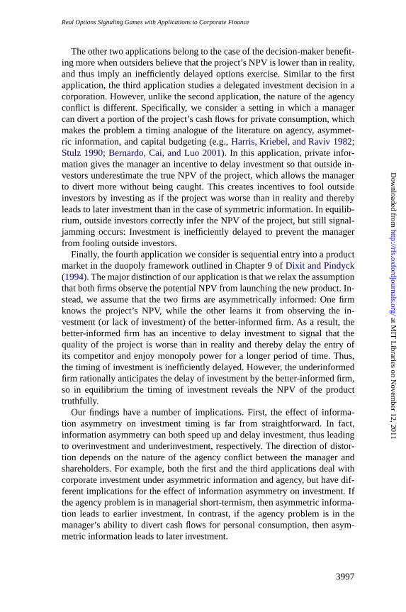
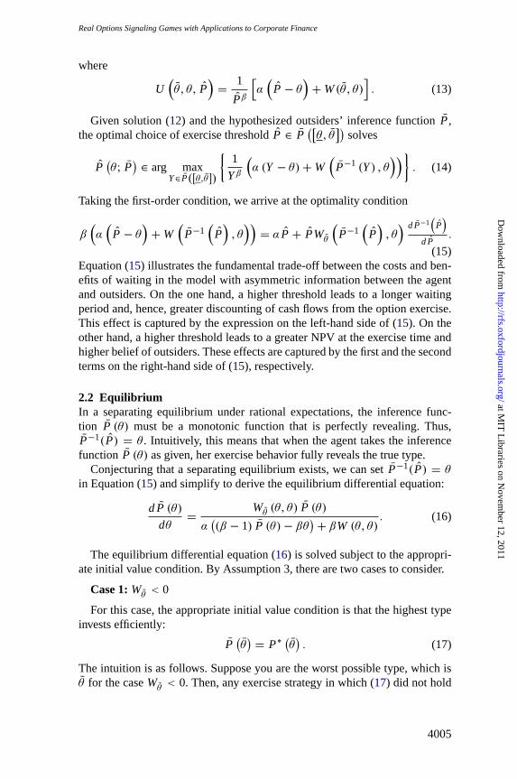
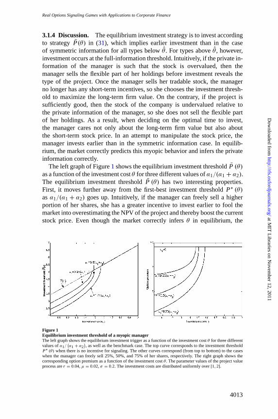
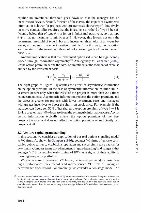
The left graph of Figure1 shows the equilibrium investment thresholdP (θ)as a function of the investment costθ for three different values ofα1/(α1 + α2).The equilibrium investment thresholdP (θ) has two interesting properties.First, it moves further away from the first-best investment thresholdP∗ (θ)asα1/(α1 + α2) goes up. Intuitively, if the manager can freely sell a higherportion of her shares, she has a greater incentive to invest earlier to fool themarket into overestimating the NPV of the project and thereby boost the currentstock price. Even though the market correctly infersθ in equilibrium, the
Figure 1Equilibrium investment threshold of a myopic managerThe left graph shows the equilibrium investment trigger as a function of the investment costθ for three differentvalues ofα1/
(α1 + α2
), as well as the benchmark case. The top curve corresponds to the investment threshold
P∗ (θ) when there is no incentive for signaling. The other curves correspond (from top to bottom) to the caseswhen the manager can freely sell 25%, 50%, and 75% of her shares, respectively. The right graph shows thecorresponding option premium as a function of the investment costθ . The parameter values of the project valueprocess arer = 0.04, μ = 0.02, σ = 0.2. The investment costs are distributed uniformly over[1,2].
4013
at MIT
Libraries on N
ovember 12, 2011
http://rfs.oxfordjournals.org/D
ownloaded from
TheReview of Financial Studies / v 24 n 12 2011
equilibrium investment threshold goes down so that the manager has noincentives to deviate. Second, for each of the curves, the impact of asymmetricinformation is lower for projects with greater costs (lower types). Intuitively,incentive compatibility requires that the investment threshold of typeθ be suf-ficiently below that of typeθ + ε for an infinitesimal positiveε, so that typeθ + ε has no incentive to mimic typeθ . However, this lowers not only theinvestment threshold of typeθ , but also investment thresholds of all types be-low θ , as they must have no incentive to mimicθ . In this way, the distortionaccumulates, so the investment threshold of a lower type is closer to the zeroNPV rule.
Another implication is that the investment option value can be significantlyeroded through information asymmetry.26 Analogouslyto Grenadier(2002),let the option premium define the NPV of investment at the moment of exercisedivided by the investment cost:
O P
(θ,
α1
α1 + α2
)=
P (θ)− θ
θ. (34)
The right graph of Figure1 quantifies the effect of asymmetric informationon the option premium. In the case of symmetric information, equilibrium in-vestment occurs only when the NPV of the project is more than 2.41 timesits investment cost. Asymmetric information reduces the option premium, andthe effect is greater for projects with lower investment costs and managerswith greater incentives to boost the short-run stock price. For example, if themanager can freely sell 50% of her shares, the option premium of typeθ = 1 is1.41, a greater than 40% decrease from the symmetric information case. Asym-metric information typically affects the option premium of the bestprojects the most and does not affect the option premium of sufficiently badprojects at all.
3.2 Venture capital grandstandingIn this section, we consider an application of our real options signaling modelto VC firms. As shown inGompers(1996), younger VC firms often take com-panies public earlier to establish a reputation and successfully raise capital fornew funds. Gompers terms this phenomenon “grandstanding”and suggests thatyounger VC firms employ early timing of IPOs as a signal of their ability toform higher-quality portfolios.
We characterize experienced VC firms (the general partners) as those hav-ing a performance track record, and inexperienced VC firms as having noperformance track record. For simplicity, we consider a two-stage model. An
26 Previous research (Williams 1993; Grenadier 2002) has demonstrated that the value of the option to invest canbe significantly eroded because of competitive pressure in the industry. This application shows that if a portionof the manager’s utility comes from the short-term stock price, then the value of the option to invest can beeroded even in monopolistic industries, as long as the manager is better informed about the investment projectthan the market.
4014
at MIT
Libraries on N
ovember 12, 2011
http://rfs.oxfordjournals.org/D
ownloaded from
RealOptions Signaling Games with Applications to Corporate Finance
inexperienced VC firm invests outsiders’ (limited partners’) money in the firstround. The firm then chooses when to allow its first-round portfolio companiesto go public. When such an IPO takes place, the firm becomes experiencedand raises money for the second round. Notably, its ability to attract outsiders’funds in the second round will depend on the belief of outsiders of its skill, asinferred from the results of the first round.
We shall work backward and initially consider the second round (an experi-enced VC firm), to be followed by the first round (an inexperienced VC firm).
3.2.1 The experienced VC firm. In the second round of financing,I2 dol-larsare invested, whereI2 is endogenized below. The value of the fund, shouldit choose to go public at timet , is
(P2(t)− θ + ε2) H(I2), (35)
whereP2 (t) is the publicly observable component of value,θ is the privatelyobserved value of the VC firm’s skill, andε2 is a zero-mean shock, whichcorresponds to the contribution of luck. Only the VC firm knows the valueof its skill θ (lower θ means higher skill); the outside investors must use aninferred value ofθ .27 While outside investors cannot disentangle the mix ofskill and luck, the VC firm learns the realization of luck,ε2, upon investment.Finally, H(.) describesthe nature of the returns to scale on investment. Toaccount for declining returns to scale (that is, at some point the firm runs outof good project opportunities), we impose the Inada conditions:H(0) = 0,H ′ > 0, H ′′ < 0, H ′ (0) = ∞, andH ′ (∞) = 0. In addition, we assume thatH ′′′ is continuous.
We assume that the VC firm receives as compensation a fractionα of theproceeds from an IPO (or a similar liquidity event).28 TheVC firm decides ifand when to allow the portfolio to go public. Thus, the timing of the IPO isa standard option exercise problem where the expected payoff to the VC firmupon exercise is
α (P2 (t)− θ) H(I2). (36)
Theoptimal second-round IPO exercise trigger is thus the first-best solution:
P2 (θ) =β
β − 1θ. (37)
We now endogenize the second-round level of investment. At the beginningof the second round, the limited partners decide how much capital to contribute
27 The model can be extended to a more realistic, albeit less tractable, setting in which the firm has imperfectknowledge of its ability. This extended model has similar results and intuition, as long as the firm is betterinformed about its ability than investors.
28 For purposes of this application, we take the compensation structure of the general partner as given. This struc-ture is quite similar to the observed industry practice (e.g.,Metrick and Yasuda 2010).
4015
at MIT
Libraries on N
ovember 12, 2011
http://rfs.oxfordjournals.org/D
ownloaded from
TheReview of Financial Studies / v 24 n 12 2011
to the fund. We normalize the value of the publicly observable component uponthe initiation of the second round,P2 (0), to one, so thatP2(t) representsthevalue growth over the initial cost.29 The limited partners choose the level ofinvestmentI2 so as to maximize the expected value of their net investment.Because the limited partners do not observe the VC firm’s skillθ , they useinferenceθ based on the IPO signal from the first round. For a givenθ , thelimited partners chooseI2 by solving the following optimization problem:
maxI2
(1 − α)
P2
(θ)
− θ
P2
(θ)β H (I2)− I2
. (38)
TheInada conditions guarantee that the optimal level of investment,I2
(θ), is
given by the first-order condition:
I2
(θ)
= H ′−1
[(β
β − 1
)β β − 1
1 − αθβ−1
]
. (39)
I2
(θ)
is strictly decreasing inθ , meaning that the limited partners invest more
if they believe that the general partner is more skilled.Thus, for givenθ andθ , the value of the second-round financing to the VC
firm is
αP2 (θ)− θ
P2 (θ)β
H(
I2
(θ)). (40)
Importantly, this value is a decreasing function of the inferred typeθ . Hence,the VC firm benefits from higher inferred skill.
3.2.2 The inexperienced VC firm. Now, let us consider the first round.30
The fund hasI1 invested, and the VC firm must choose if and when to allowits portfolio to go public. The payoff to the VC firm is the sum of their share ofthe proceeds from going public and the expected utility of the second-round fi-nancing. The proceeds from going public at timet are(P1 (t)− θ + ε1) H (I1),whereε1 is a zero-mean shock, while the value of the second-round financingis given by (40). Thus, for an IPO trigger ofP1, the expected payoff to the VCfirm is
α(
P1 − θ)
H(I1)+ αP2 (θ)− θ
P2 (θ)β
H(
I2
(θ)), (41)
29 Becauseof this normalization, we assume that the parameters of the model are such thatP(θ)> 1.
30 For simplicity, we assume that the skill parameterθ of the VC firm is the same in both rounds. The model canbe extended to the case of different, but correlated, skill levels across rounds. In such a case, in equilibrium thetiming of investment is an imperfect rather than perfect signal about the general partner’s talent.
4016
at MIT
Libraries on N
ovember 12, 2011
http://rfs.oxfordjournals.org/D
ownloaded from
RealOptions Signaling Games with Applications to Corporate Finance
where I2
(θ)
is given by (39). For simplicity, we normalizeH (I1) to 1. We
can thus see that this problem corresponds to the general model with31
W(θ , θ
)= α
P2 (θ)− θ
P2 (θ)β
H(
I2
(θ)), (42)
whereWθ < 0. Assuming that the lowest possible type is not too low,
θ >β − 1
β
(
θ −W(θ , θ
)
α
)
, (43)
the single-crossing condition is satisfied.32 Thus, the separating equilibriumthe investment triggerP1 (θ) is given by
dP1 (θ)
dθ=
P1 (θ) I ′2 (θ) / (1 − α)
(β − 1) P1 (θ)− βθ + β P2(θ)−θP2(θ)
β H (I2 (θ)), (44)
solved subject to the boundary condition that typeθ invests at the full-information threshold:33
P1(θ)
=β
β − 1
(
θ −P2(θ)− θ
P2(θ)β H
(I2(θ)))
. (45)
3.2.3 Discussion. The timing of the IPO of the inexperienced firm charac-terized by (44)–(45) has several intuitive properties. First, the inexperiencedfirm takes the portfolio company public earlier than optimal. Because the in-experienced firm is better informed about its talent than the limited partners,the inexperienced firm has an incentive to manipulate the timing of the IPOto make the limited partners believe that its quality is higher. Because an ear-lier IPO is a signal of higher quality, it will go public earlier than in the caseof symmetric information. In equilibrium, signal-jamming occurs: The limitedpartners correctly conjecture that the VC firm goes public earlier than optimal,so the type of the general partner is revealed. The degree of inefficient timing is
31 Notethat if the limited partners observe the proceeds from the first round, then they may also use this informationto inferθ . However, this does not affect the model, because the proceeds are a noisier signal of the firm’s privateinformation than the timing. Indeed, the proceeds reveal the value ofθ − ε1, while the timing in a separatingequilibrium revealsθ .
32 It can be easily checked that functionW(θ , θ
)in this application also satisfies Assumptions 1–4, provided that
the optimal IPO threshold in the first round in the case of symmetric information is finite.
33 To ensure that none of the types does an IPO immediately, we make an assumption that the initial valueP (0) isbelow P1
(θ). Then, the unique separating equilibrium investment threshold is defined as an increasing function,
which solves (44) subject to (45).
4017
at MIT
Libraries on N
ovember 12, 2011
http://rfs.oxfordjournals.org/D
ownloaded from
The Review of Financial Studies / v 24 n 12 2011
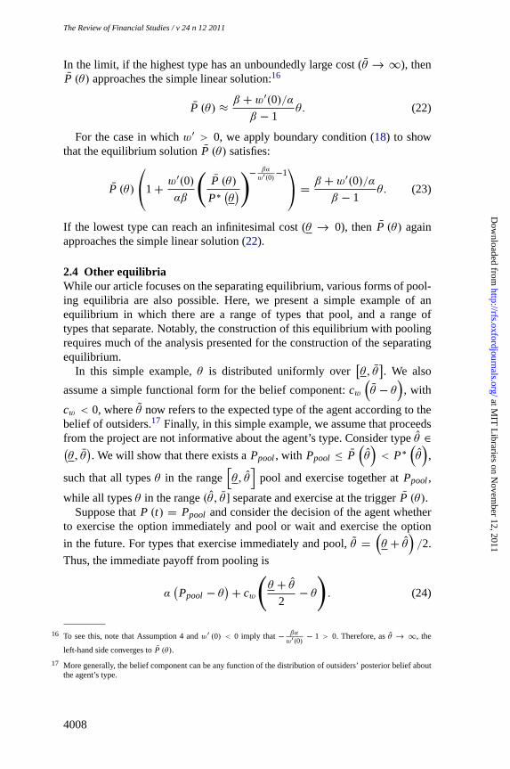
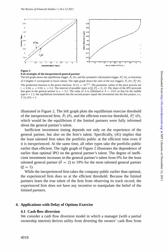
Figure 2Exit strategies of the inexperienced general partnerThe left graph shows the equilibrium trigger,P1 (θ), and the symmetric information trigger,P∗
1 (θ), as functions
of θ (higherθ corresponds to lower talent). The right graph shows the ratio of the two triggers,P1 (θ) /P∗1 (θ).
The production function is the power function:H (I ) = AI2/3. The parameter values of the price process arer = 0.04, μ = 0.02, σ = 0.2. The interval of possible types is
[θ, θ
]= [1,2]. The share of the IPO proceeds
that goes to the general partner isα = 0.2. The value ofA is calibrated atA = 3.015 so that for the middletypeθ = 1.5, the equilibrium investment into the second project equals the investment into the first project, i.e.,F(I2 (θ)
)= 1.
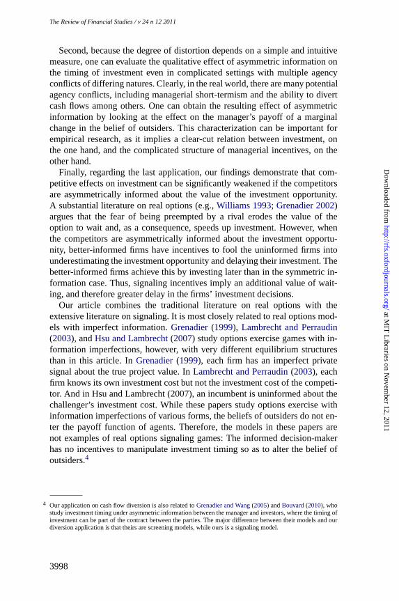
illustrated in Figure2. The left graph plots the equilibrium exercise thresholdof the inexperienced firm,P1 (θ), and the efficient exercise threshold,P∗
1 (θ),which would be the equilibrium if the limited partners were fully informedabout the general partner’s talent.
Inefficient investment timing depends not only on the experience of thegeneral partner, but also on the firm’s talent. Specifically, (45) implies thatthe least talented firm takes the portfolio public at the efficient time even ifit is inexperienced. At the same time, all other types take the portfolio publicearlier than efficient. The right graph of Figure2 illustrates the dependence ofearlier than optimal IPO on the general partner’s talent. The degree of ineffi-cient investment increases in the general partner’s talent from 0% for the leasttalented general partner (θ = 2) to 19% for the most talented general partner(θ = 1).
While the inexperienced firm takes the company public earlier than optimal,the experienced firm does so at the efficient threshold. Because the limitedpartners learn the true talent of the firm from observing its track record, theexperienced firm does not have any incentive to manipulate the belief of thelimited partners.
4. Applications with Delay of Options Exercise
4.1 Cash flow diversionWe consider a cash flow diversion model in which a manager (with a partialownership interest) derives utility from diverting the owners’ cash flow from
4018
at MIT
Libraries on N
ovember 12, 2011
http://rfs.oxfordjournals.org/D
ownloaded from

RealOptions Signaling Games with Applications to Corporate Finance
investment for personal consumption.34 Thus,in this case, the manager wouldlike shareholders to believe that the investment cost is higher than in reality.We begin by providing a costly state verification model to endogenize the man-ager’s cash flow diversion utility. Then, conditional on the manager’s diversionincentives, we move on to modeling the manager’s optimal investment strategy.
The assumption that a portion of project value is observed only by themanager and not verifiable by the owners is common in the capital budget-ing literature. This information asymmetry invites a host of agency issues.Harris, Kriebel, and Raviv(1982) posit that managers have incentives to un-derstate project payoffs and to divert the free cash flow to themselves. In theirmodel, such value diversion takes the form of the manager reducing her level ofeffort. Stulz(1990),Harris and Raviv(1996),Bernardo, Cai, and Luo(2001),andMalenko(2011) model the manager as having preferences for perquisiteconsumption or empire-building. In these models, the manager has incentivesto divert free cash flows to inefficient investments or to excessive perquisites.Grenadier and Wang(2005) apply an optimal contracting approach to en-sure against diversion and to provide an incentive for the manager to exerciseoptimally.
4.1.1 Costly state verification model. Suppose that the manager can divertany amountd from the project value before the noiseε is realized.35 As isstandard in the literature (e.g.,DeMarzo and Sannikov 2006), diversion is po-tentially wasteful, so that the manager receives only a fractionλ ∈ [0,1] of thediverted value. After the project cash flow ofP − θ − d + ε is realized, theshareholders either verify whether the manager diverted or not. Verificationcostsc > 0. If the shareholders verify that the manager diverted fundsd fromthe firm, the manager is required to return them to the firm.36 Thus,the timingof the interactions is the following. First, the manager decides when to exercisethe investment option. Then, after the investment has been made but before thecash flow is realized, the shareholders decide on the verification strategy.37
As in traditional costly state verification models (Townsend 1979; Gale andHellwig 1985), the investors (shareholders, in our case) can commit to the de-terministic verification strategy. After that, but before observing the noiseε,the manager decides how much to divert. Finally, the project’s cash flow ofP − θ − d + ε is realized, and the shareholders either verify the manager or
34 We take the structure of the manager’s compensation contract as given. In a more general model, the manager’sownership stake could itself be endogenous.
35 We make an assumption that the manager is not allowed to inject her own funds into the firm. This assumptionsimplifies the solution but is not critical, as long as injection is not too profitable.
36 The model can be extended by allowing the shareholders to impose a non-pecuniary cost on the manager ifdiversion is verified.
37 While we assume that the proceeds from the project realize an instant after the investment has been made, themodel can be extended to include the time to build feature (e.g., as inMajd and Pindyck 1987).
4019
at MIT
Libraries on N
ovember 12, 2011
http://rfs.oxfordjournals.org/D
ownloaded from
TheReview of Financial Studies / v 24 n 12 2011
not,according to the prespecified verification strategy. LetΨ andψ denote thecumulative distribution and density functions ofε, respectively. Assume thatψ is C2.
In Appendix B, we demonstrate that any optimal verification strategy takesthe form of verifying the manager if and only if the difference between theexpected and the realized cash flows is greater than a particular threshold. Inother words, for somev, verification occurs if and only ifP − θ − d + ε −(
P − θ)< v, or, equivalently,ε < v − θ + θ + d. Let us initially choose any
verification parameterv and determine the manager’s optimal diversion strat-egy in response. Then, conditional on this managerial response, we determinethe shareholders’ optimal choice ofv.
Consider a manager of typeθ that is inferred by the market as typeθ .If the manager divertsd, she expects to be verified with probability
Ψ(v − θ + θ + d
), in which case there is no impact on her payoff, as the
diverted cash flow is returned to the firm. However, she is not verified withprobability 1− Ψ
(v − θ + θ + d
), in which case she gains fractionλ of the
diverted cash flow for her private benefit and loses fractionα due to her own-ership position. Hence, the manager’s problem is
maxd≥0
{(λ− α) d
(1 − Ψ
(v − θ + θ + d
))}. (46)
Clearly, if α ≥ λ, then the manager does not divert anything:d = 0.38 Now,consider the caseα < λ. Assuming that the hazard rate of the distribution ofε,hψ (z) ≡ ψ (z) / (1 − Ψ (z)), is increasing, (46) has a unique solutiond∗ thatsatisfies
d∗hψ(v − θ + θ + d∗
)= 1. (47)
The solution d∗ is a decreasing function ofv − θ + θ . Let us denote this
functional dependence byD(v − θ + θ
).
Given the manager’s response to verification rulev, we now solve for theshareholders’ optimal choice ofv. Under the shareholders’ information set,they expect the manager to divertD (v) and estimate the probability of veri-fication atΨ (v + D (v)). For any choice ofv, the shareholders lose 1− α ofthe diverted cash flow when verification does not occur, and pay costc whenverification occurs. Thus, the optimal verification parameterv∗ is
v∗ = arg minv
{(1 − α) (1 − Ψ (v + D (v))) D (v)+ Ψ (v + D (v)) c} . (48)
38 Technically, the manager is indifferent in her choice ofd whenα = λ. However, if there is any infinitesimal butpositive fixed cost of diversion, a zero level will be chosen.
4020
at MIT
Libraries on N
ovember 12, 2011
http://rfs.oxfordjournals.org/D
ownloaded from

RealOptions Signaling Games with Applications to Corporate Finance
In summary, we have determined the manager’s diversion and shareholders’verification strategies. Ifα ≥ λ, then the manager does not divert cash flowand the shareholders do not verify the manager:d = 0, v = −∞. If α < λ,
the manager divertsD(v∗ − θ + θ
), and the shareholders verify the manager
if and only if the project’s realized cash flow falls belowv∗ + P − θ .
4.1.2 Equilibrium investment timing. Given the manager’s diversion rulederived above, her payoff from exercising the option at thresholdP, when hertype isθ and the shareholders’ belief isθ , equals
α(
P − θ)
+ max(λ− α, 0) D(v∗ − θ + θ
)
×(1 − Ψ
(v∗ − θ + θ + D
(v∗ − θ + θ
))). (49)
Thus,this problem is a special case of the general model with
W(θ , θ
)= max(λ− α, 0) D
(v∗ − θ + θ
)
×(1 − Ψ
(v∗ − θ + θ + D
(v∗ − θ + θ
))). (50)
Notice that for λ > α, Wθ
(θ , θ
)> 0, meaning that the application corre-
sponds to Case 2 of the general model. Intuitively, as the shareholders becomemore pessimistic about the project’s value, the manager diverts more and getsverified less frequently.
Using the solution analogous to (23), we can expressP (θ) implicitly as thesolution to the following equation:39
1+max(λ− α, 0) (1 − Ψ (v∗ + D (v∗)))
αβ
(P (θ)
P∗(θ)
)− βαmax(λ−α,0)(1−Ψ(v∗+D(v∗)))
−1
=β + max
(λα − 1,0
)(1 − Ψ (v∗ + D (v∗)))
β − 1
×θ − max
(λα − 1,0
)D (v∗) (1 − Ψ (v∗ + D (v∗)))
P (θ), (51)
39 For P (θ) to correspond to the separating equilibrium, we need to ensure that the parameters of the
application satisfy Assumption 5. A sufficient condition isα >
[maxz∈
[θ−θ ,θ−θ
] w′′(z)w′(z)
]×
(β−1β α P
(θ)− αθ + w
(θ − θ
))− w′ (θ − θ
). Analogously to (43), this condition is always satisfied if the
interval[θ, θ
]is not too wide. Assumptions 1–4 are always satisfied byW
(θ , θ
)in this application, as long as
P∗ (θ)> 0, as given below.
4021
at MIT
Libraries on N
ovember 12, 2011
http://rfs.oxfordjournals.org/D
ownloaded from
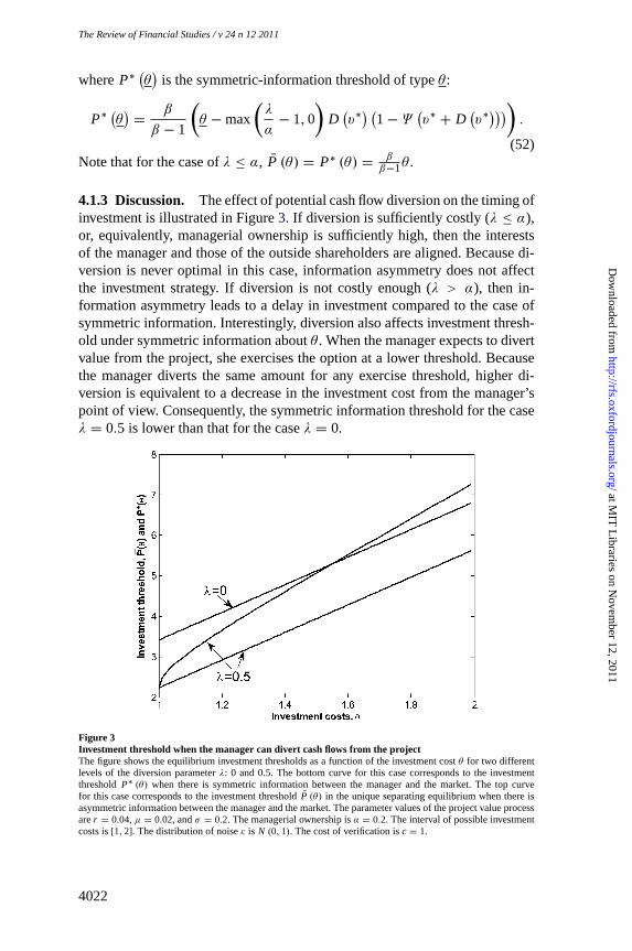
The Review of Financial Studies / v 24 n 12 2011
whereP∗(θ)
is the symmetric-information threshold of typeθ :
P∗ (θ)
=β
β − 1
(θ − max
(λ
α− 1,0
)D(v∗) (1 − Ψ
(v∗ + D
(v∗)))
).
(52)Note that for the case ofλ ≤ α, P (θ) = P∗ (θ) = β
β−1θ .
4.1.3 Discussion. The effect of potential cash flow diversion on the timing ofinvestment is illustrated in Figure3. If diversion is sufficiently costly (λ ≤ α),or, equivalently, managerial ownership is sufficiently high, then the interestsof the manager and those of the outside shareholders are aligned. Because di-version is never optimal in this case, information asymmetry does not affectthe investment strategy. If diversion is not costly enough (λ > α), then in-formation asymmetry leads to a delay in investment compared to the case ofsymmetric information. Interestingly, diversion also affects investment thresh-old under symmetric information aboutθ . When the manager expects to divertvalue from the project, she exercises the option at a lower threshold. Becausethe manager diverts the same amount for any exercise threshold, higher di-version is equivalent to a decrease in the investment cost from the manager’spoint of view. Consequently, the symmetric information threshold for the caseλ = 0.5 is lower than that for the caseλ = 0.
Figure 3Investment threshold when the manager can divert cash flows from the projectThe figure shows the equilibrium investment thresholds as a function of the investment costθ for two differentlevels of the diversion parameterλ: 0 and 0.5. The bottom curve for this case corresponds to the investmentthresholdP∗ (θ) when there is symmetric information between the manager and the market. The top curvefor this case corresponds to the investment thresholdP (θ) in the unique separating equilibrium when there isasymmetric information between the manager and the market. The parameter values of the project value processarer = 0.04, μ = 0.02, andσ = 0.2. The managerial ownership isα = 0.2. The interval of possible investmentcosts is[1,2]. The distribution of noiseε is N (0,1). The cost of verification isc = 1.
4022
at MIT
Libraries on N
ovember 12, 2011
http://rfs.oxfordjournals.org/D
ownloaded from
RealOptions Signaling Games with Applications to Corporate Finance
In Figure3, distortion in the investment threshold due to information asym-metry is greater for projects of lower quality. This result contrasts with theresults in the previous two applications. There, the exercise trigger is alteredin a way that the manager has no incentives to mimic a lower type. As a re-sult, distortion in the exercise timing does not exist for the highest types (worstprojects) and exists for lower types. In contrast, now the exercise trigger isaltered in a way that the manager has no incentives to mimic a higher type. Asa result, distortion in exercise timing does not exist for the lowest types (bestprojects) and exists for higher types.
4.2 Strategic product market competitionAnother example of a real options signaling game in which asymmetric in-formation delays options exercise is the strategic entry into a product market.Specifically, consider the entry decisions of two firms that are asymmetricallyinformed about the value of a new product. Firm 1 knows the investment costθ , while firm 2 does not. For example, firm 1 may have greater experiencein similar product introductions or may be the industry’s technology leader.When there is only one firm in the industry, it receives a monopoly profit flowof P(t). When there are two firms in the industry, each receives a duopoly
profit flow of λP(t), whereλ ∈(1 − 1
β , 1).40 We derive the Bayes-Nash
separating equilibrium in two different versions of the game: when firm 1 isthe designated leader (the “Stackelberg equilibrium”) and when the roles ofthe two firms are determined endogenously (the “Cournot equilibrium”). Wefocus on the limiting caseθ → 0 to obtain the closed-form solutions.
Product market competition in a real options framework has been frequentlyanalyzed in the literature.Leahy(1993),Williams (1993), andGrenadier(2002)study simultaneous investment by symmetric firms in a competitive equilib-rium. Novy-Marx (2007) looks at a similar problem with heterogeneous firms.Grenadier(1996),Weeds(2002), andLambrecht and Perraudin(2003) studysequential investment in leader-follower games. We follow the simple duopolyframework outlined in Chapter 9 ofDixit and Pindyck(1994). The key dis-tinction with the perfect information framework in Dixit and Pindyck (1994)is that one firm knows the investment cost, while the other attempts to infer itthrough the informed firm’s investment decision. The main insight is that theinformed firm will delay its investment to signal to the uniformed firm that thecost is higher than in reality, thereby attempting to delay the uniformed firm’sentrance and enjoy monopoly profits for a longer period. In equilibrium, thiseffort to deceive will fail, but the informed firm’s entry will still be delayedrelative to the full-information entry time.41
40 Essentially, the assumption thatλ > 1 − 1β rulesout any overwhelming influence of monopoly power.
41 Lambrechtand Perraudin(2003) andHsu and Lambrecht(2007) are also related to the model in this section.They study competition between two firms for an investment opportunity when the information structure is
4023
at MIT
Libraries on N
ovember 12, 2011
http://rfs.oxfordjournals.org/D
ownloaded from

TheReview of Financial Studies / v 24 n 12 2011
Theinvestment decision of firm 1 depends on the degree of pressure it feelsdue to firm 2’s potential preemption. We will begin with the assumption ofa Stackelberg equilibrium (where there is no potential preemption) and thenshow the extension to a Cournot equilibrium (where preemption by firm 2 ispossible).
4.2.1 The Stackelberg equilibrium. Let us work backward and begin byconsidering the situation when firm 1 has already invested. Firm 2 has usedfirm 1’s entry time to make an inference aboutθ , denoted byθ . Given itsinferred signal, firm 2 holds a standard real option whose expected payoff atexercise isλP
r −μ − θ . Firm 2 will thus enter at the first instant whenP (t) equals
or exceedsPF
(θ), given by
PF
(θ)
=β
β − 1
r − μ
λθ. (53)
Now, consider the entry of firm 1. Upon payment ofθ at exercise, firm 1begins receiving the monopoly profit flow ofP(t), which is then reduced toλP(t) once firm 2 enters. Thus, for a given typeθ , firm 2’s belief θ , and theentry triggerPL , the payoff to firm 1 at the moment of entry is
PLr −μ − θ −
(PL
PF
(θ)
)βPF
(θ)(1−λ)
r −μ , for PL ≤ PF
(θ),
λPLr −μ − θ, for PL > PF
(θ).
(54)
Let PL (θ) denotethe equilibrium entry threshold of firm 1 in the Stackelbergcase. Conjecture thatPL (θ) ≤ PF (θ), which is verified in Appendix B. Then,from (54), we can see that the payoff from exercise can be written as
α(
PL − θ)
+ W(PL , θ , θ), (55)
whereα = 1r −μ and
W(PL , θ , θ) = −PβL α (1 − λ) PF
(θ)1−β
− (1 − α) θ. (56)
Note that the belief component of this payoff is not a special case of themodel outlined in Section1, given thatPL is included as an argument. InAppendix B, we show that this slight difference in the functions can be easily
imperfect.In Lambrecht and Perraudin(2003), each firm knows its own investment cost but not the cost of itscompetitor. InHsu and Lambrecht(2007), the investment cost of one firm (the incumbent) is public knowledge,while the investment cost of the other firm is known only to itself.
4024
at MIT
Libraries on N
ovember 12, 2011
http://rfs.oxfordjournals.org/D
ownloaded from
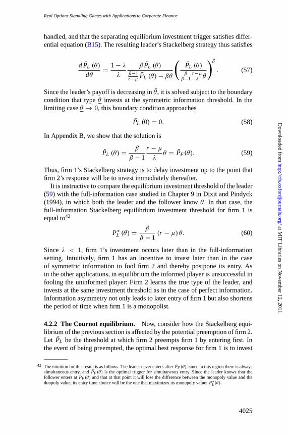
RealOptions Signaling Games with Applications to Corporate Finance
handled,and that the separating equilibrium investment trigger satisfies differ-ential equation (B15). The resulting leader’s Stackelberg strategy thus satisfies
dPL (θ)
dθ=
1 − λ
λ
β PL (θ)β−1r −μ PL (θ)− βθ
(PL (θ)ββ−1
r −μλ θ
)β
. (57)
Sincethe leader’s payoff is decreasing inθ , it is solved subject to the boundarycondition that typeθ invests at the symmetric information threshold. In thelimiting caseθ → 0, this boundary condition approaches
PL (0) = 0. (58)
In Appendix B, we show that the solution is
PL (θ) =β
β − 1
r − μ
λθ = PF (θ). (59)
Thus, firm 1’s Stackelberg strategy is to delay investment up to the point thatfirm 2’s response will be to invest immediately thereafter.
It is instructive to compare the equilibrium investment threshold of the leader(59) with the full-information case studied in Chapter 9 in Dixit and Pindyck(1994), in which both the leader and the follower knowθ . In that case, thefull-information Stackelberg equilibrium investment threshold for firm 1 isequal to42
P∗L (θ) =
β
β − 1(r − μ) θ. (60)
Sinceλ < 1, firm 1’s investment occurs later than in the full-informationsetting. Intuitively, firm 1 has an incentive to invest later than in the caseof symmetric information to fool firm 2 and thereby postpone its entry. Asin the other applications, in equilibrium the informed player is unsuccessful infooling the uninformed player: Firm 2 learns the true type of the leader, andinvests at the same investment threshold as in the case of perfect information.Information asymmetry not only leads to later entry of firm 1 but also shortensthe period of time when firm 1 is a monopolist.
4.2.2 The Cournot equilibrium. Now, consider how the Stackelberg equi-librium of the previous section is affected by the potential preemption of firm 2.Let PL be the threshold at which firm 2 preempts firm 1 by entering first. Inthe event of being preempted, the optimal best response for firm 1 is to invest
42 Theintuition for this result is as follows. The leader never enters afterPF (θ), since in this region there is alwayssimultaneous entry, andPF (θ) is the optimal trigger for simultaneous entry. Since the leader knows that thefollower enters atPF (θ) andthat at that point it will lose the difference between the monopoly value and theduopoly value, its entry time choice will be the one that maximizes its monopoly value:P∗
L (θ).
4025
at MIT
Libraries on N
ovember 12, 2011
http://rfs.oxfordjournals.org/D
ownloaded from
TheReview of Financial Studies / v 24 n 12 2011
at the first time whenP (t) equals or exceeds the optimal follower’s thresholdPF (θ).
Given any preemption threshold,PL , we can compute the conditionalexpected value of firm 2 before either firm invests. LetPM (t) denotethe his-torical maximum ofP (t) as of timet . If firm 1 has not invested before timet ,firm 2 learns thatθ is such thatPL (θ) > PM (t), i.e., θ > β−1
βλ
r −μ PM (t).There are two ranges ofθ : In the upper range, firm 2 enters first, and inthe lower range, both firms enter simultaneously. For the case in whichθ >β−1β
λr −μ PL , PL< PL (θ) andthus firm 2 preempts firm 1 by investing atPL .
For the case in whichθ ≤ β−1β
λr −μ PL , PL ≥ PL (θ) andthus firm 1 enters
at the Stackelberg triggerPL (θ), where firm 2 will then inferθ and immedi-ately enter. Combining these cases, firm 2’s value, conditional onP and PM ,is equal to
∫ β−1β
λr −μ PL
β−1β
λr −μ PM
(P
PF (θ)
)β (λPF (θ)
r −μ − θ)
φ(θ)
1−Φ(β−1β
λr −μ PM
)dθ
+∫ θβ−1β
λr −μ PL
(PPL
)β ( PLr −μ −
(PL
PF (θ)
)β(1−λ)PF (θ)
r −μ − θ
)φ(θ)
1−Φ(β−1β
λr −μ PM
)dθ.
(61)The optimal preemption strategy is to invest at thePL that maximizes(61). The corresponding first-order condition is43
PL =β
β − 1
E[θ |θ ≥ β−1
βλ
r −μ PL
]
r − μ. (62)
In other words, the equilibrium preemption trigger equals the expected full-information Stackelberg trigger, conditional on preemption. In Appendix B,we show that the optimal preemption threshold,PL , is always between 0 andPF(θ). In particular, assuming thatθφ (θ) / (1 −Φ (θ)) is increasing inθ ,
Equation (62) has a unique solution, which determinesPL .44
We can now fully characterize the Cournot equilibrium outcome. Firm 2 at-tempts to preempt firm 1 by investing at triggerPL , which is implicitly givenby (62). If θ is such thatPL < PL(θ), then firm 2 invests first atPL , and firm1 invests later atPF (θ) = PL(θ). Alternatively, if θ is such thatPL ≥ PL(θ),then both firms invest simultaneously at triggerPL(θ). Thus, in all cases theinformed firm invests later than it would in the case of full information. Thisdelay is due to its strategic incentive to artificially inflate firm 1’s inferredestimate ofθ .
43 Notethat if θ is such thatPL (θ) > PL , it is not optimal for firm 1 to preempt firm 2 by investing at a thresholdbelow PL . Indeed, if firm 1 invested atP < PL , firm 2 would respond by investing immediately after firm 1,as it would perceive thatθ is such thatPL (θ) = PF (θ) = P. As a result, firm 1 does not gain any monopolypower from investing belowPL , so its best response to the preemptive strategy of firm 2 is to invest atPF (θ).
44 Intuitively, this assumption means that the density of distribution does not have abrupt kinks. It is satisfied formost standard distributions.
4026
at MIT
Libraries on N
ovember 12, 2011
http://rfs.oxfordjournals.org/D
ownloaded from
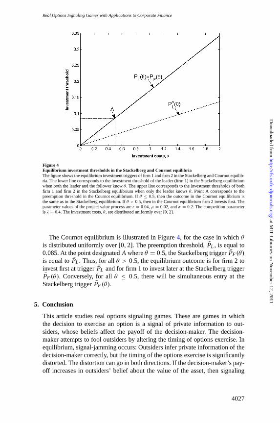
Real Options Signaling Games with Applications to Corporate Finance
Figure 4Equilibrium investment thresholds in the Stackelberg and Cournot equilibriaThe figure shows the equilibrium investment triggers of firm 1 and firm 2 in the Stackelberg and Cournot equilib-ria. The lower line corresponds to the investment threshold of the leader (firm 1) in the Stackelberg equilibriumwhen both the leader and the follower knowθ . The upper line corresponds to the investment thresholds of bothfirm 1 and firm 2 in the Stackelberg equilibrium when only the leader knowsθ . Point A corresponds to thepreemption threshold in the Cournot equilibrium. Ifθ ≤ 0.5, then the outcome in the Cournot equilibrium isthe same as in the Stackelberg equilibrium. Ifθ > 0.5, then in the Cournot equilibrium firm 2 invests first. Theparameter values of the project value process arer = 0.04, μ = 0.02, andσ = 0.2. The competition parameteris λ = 0.4. The investment costs,θ , are distributed uniformly over[0,2].
The Cournot equilibrium is illustrated in Figure4, for the case in whichθis distributed uniformly over[0,2]. The preemption threshold,PL , is equal to0.085. At the point designatedA whereθ = 0.5, the Stackelberg triggerPF (θ)is equal toPL . Thus, for allθ > 0.5, the equilibrium outcome is for firm 2 toinvest first at triggerPL and for firm 1 to invest later at the Stackelberg triggerPF (θ). Conversely, for allθ ≤ 0.5, there will be simultaneous entry at theStackelberg triggerPF (θ).
5. Conclusion
This article studies real options signaling games. These are games in whichthe decision to exercise an option is a signal of private information to out-siders, whose beliefs affect the payoff of the decision-maker. The decision-maker attempts to fool outsiders by altering the timing of options exercise. Inequilibrium, signal-jamming occurs: Outsiders infer private information of thedecision-maker correctly, but the timing of the options exercise is significantlydistorted. The distortion can go in both directions. If the decision-maker’s pay-off increases in outsiders’ belief about the value of the asset, then signaling
4027
at MIT
Libraries on N
ovember 12, 2011
http://rfs.oxfordjournals.org/D
ownloaded from
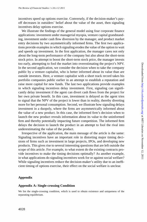
TheReview of Financial Studies / v 24 n 12 2011
incentives speed up options exercise. Conversely, if the decision-maker’s pay-off decreases in outsiders’ belief about the value of the asset, then signalingincentives delay options exercise.
We illustrate the findings of the general model using four corporate financeapplications: investment under managerial myopia, venture capital grandstand-ing, investment under cash flow diversion by the manager, and product marketentry decisions by two asymmetrically informed firms. The first two applica-tions provide examples in which signaling erodes the value of the option to waitand speeds up investment. In the first application, the manager cares not onlyabout the long-term performance of the company but also about the short-termstock price. In attempt to boost the short-term stock price, the manager investstoo early, attempting to fool the market into overestimating the project’s NPV.In the second application, we consider the decision when to take the companypublic by a venture capitalist, who is better informed about its value than areoutside investors. Here, a venture capitalist with a short track record takes hisportfolio companies public earlier in an attempt to establish a reputation andraise more capital for new funds. The last two applications provide examplesin which signaling incentives delay investment. First, signaling can signifi-cantly delay investment if the agent can divert cash flows from the project forher own private benefit. In this case, investment is delayed as the agent triesto signal that the NPV of the project is lower than in reality, thereby divertingmore for her personal consumption. Second, we illustrate how signaling delaysinvestment in a duopoly, where the firms are asymmetrically informed aboutthe value of a new product. In this case, the informed firm’s decision when tolaunch the new product reveals information about its value to the uninformedfirm and thereby potentially impacting future competition. The informed firmdelays the decision to launch the product in an attempt to fool the rival intounderestimating the value of the product.
Irrespective of the application, the main message of the article is the same:Signaling incentives have an important role in distorting major timing deci-sions of firms such as investment in large projects, IPOs, and developing newproducts. This gives rise to several interesting questions that are left outside thescope of this article. For example, to what extent do the existing contracts pro-vide incentives to make the timing decisions optimally? As another example,in what applications do signaling incentives work for or against social welfare?While signaling incentives reduce the decision-maker’s utility due to an ineffi-cient timing of options exercise, their effect on the social welfare is unclear.
Appendix
Appendix A: Single-crossing Condition
We list the single-crossing condition, which is used to obtain existence and uniqueness of theseparating equilibrium.
4028
at MIT
Libraries on N
ovember 12, 2011
http://rfs.oxfordjournals.org/D
ownloaded from

RealOptions Signaling Games with Applications to Corporate Finance
Assumption5 (Single-crossing condition).FunctionW(θ , θ
)satisfies
Wθ
(θ , θ
)×
∂
[UP
(θ ,θ,P
)
Uθ
(θ ,θ,P
)
]
∂θ> 0 (A1)
for(θ , P
)in the graph ofP, whereU
(θ , θ, P
)is given by (13),β is given by (7), andP (θ) is
the unique increasing solution of the differential equation (16), subject to the boundary condition
(17), if Wθ
(θ , θ
)< 0, or (18), if Wθ
(θ , θ
)> 0.
The single-crossing condition ensures that if the agent does not make extra gains by misrep-resentingθ slightly, then extra gains cannot be made from a large misrepresentation. It is standardfor games of asymmetric information, both signaling and screening. Importantly, it is enough that
the single-crossing condition is satisfied for(θ , P
)in the graph ofP.
The single-crossing condition holds in all applications that we consider. As an example, belowwe verify the single-crossing condition for the venture capital grandstanding example of Section3.2. For this application, we have from (42):
W(θ , θ
)= α
P2 (θ)− θ
P2 (θ)β
H(
I2(θ)), (A2)
whereH ′ > 0, I ′2 < 0, and P2 (θ) is the full-information trigger in (37). Simplifying, we have
W(θ , θ
)= kθ1−βH
(I2(θ)), (A3)
wherek = αβ−1
(ββ−1
)−β> 0. Taking derivatives, we obtain that Assumption 5 requires that
(β − 1) Pθβ−1 − βθβ +(β−1β
)β−1H(
I2(θ))
Pθβ−1 11−α I ′
2
(θ) (A4)
is a strictly decreasing function ofθ for(θ , P
)in the graph ofP1. Taking the derivative with
respect toθ , we get the following requirement:
(β − 1)2 P − β2θ < 0 for P in the graph ofP1. (A5)
In the graph ofP1, the highest value ofP is P1(θ), which is given by (45). Therefore, a sufficient
condition for (A5) is(β − 1)2 P1
(θ)− β2θ < 0. (A6)
This is equivalent to (43) in Section 3.2. Hence, the single-crossing condition is verified.
Appendix B: Proofs
Proof of Proposition 2. We apply Theorems 1–3 fromMailath (1987) to prove the proposition.
We need to show that functionU(θ , θ, P
)satisfiesMailath’s (1987) regularity conditions:
• Smoothness:U(θ , θ, P
)is C2 on
[θ, θ
]2 × R+;
• Belief monotonicity:Uθ
never equals zero, and so is either positive or negative;
4029
at MIT
Libraries on N
ovember 12, 2011
http://rfs.oxfordjournals.org/D
ownloaded from

TheReview of Financial Studies / v 24 n 12 2011
• Type monotonicity:Uθ P never equals zero, and so is either positive or negative;
• “Strict”quasiconcavity:UP
(θ, θ, P
)= 0 has a unique solution inP, which maximizes
U(θ, θ, P
), and UPP
(θ, θ, P
)< 0 at this solution;
• Boundedness: There existsδ > 0 such that for all(θ, P
)∈[θ, θ
]×R+ UPP
(θ, θ, P
)≥
0 ⇒∣∣∣UP
(θ, θ, P
)∣∣∣ > δ.
Let us check that these conditions are satisfied for our problem. The smoothness condition is
satisfied, becauseW(θ , θ
)is C2 on
[θ, θ
]2. The belief monotonicity condition is satisfied, be-
causeWθ is either always positive or always negative. The type monotonicity condition is satisfied,because
Uθ P
(θ , θ, P
)=β(α − Wθ
(θ , θ
))
Pβ+1> 0, (B1)
asα > Wθ
(θ , θ
)by Assumption 4. As we show in Section 1.3,UP
(θ, θ, P
)= 0 has a unique
solution in P, denoted byP∗ (θ), that maximizesU(θ, θ, P
). Also,
UPP
(θ, θ, P∗ (θ)
)=
β
P∗ (θ)β+2
[α (β − 1) P∗ (θ)− (β + 1) (αθ − W (θ, θ))
](B2)
= −β (αθ − W (θ, θ))
P∗ (θ)β+2< 0.
Hence,the “strict”quasiconcavity condition is satisfied. Finally, to ensure that the boundednesscondition is satisfied, we restrict the set of potential investment thresholds to be bounded byk fromabove, wherek can be arbitrarily large. We will later show that extending the set of actions toP ∈(0,∞) neither destroys the separating equilibrium nor creates additional separating equilibria.
Notice thatUPP
(θ, θ, P
)≥ 0 implies thatαθ − W (θ, θ) ≤ Pα (β − 1)/(β + 1). Hence, for
any(θ, P
)∈[θ, θ
]× [0,k] such thatUPP
(θ, θ, P
)≥ 0,
∣∣∣UP
(θ, θ, P
)∣∣∣ = α(β−1)P−β(αθ−W(θ,θ))
Pβ+1 ≥α(β−1)P− βα(β−1)
β+1 P
Pβ+1 = α(β−1)(β+1)Pβ
≥ α(β−1)(β+1)kβ
> 0
(B3)for any arbitrarily largek. Then, the boundedness condition is satisfied.
By Mailath’s (1987) Theorems 1 and 2, any separating equilibriumP (θ) is continuous, dif-ferentiable, satisfies Equation (16), anddP/dθ has the same sign asU
θ P . BecauseUθ P > 0,
P (θ) is an increasing function ofθ . Let P denote the solution to the following restricted ini-tial value problem: Equation (16), subject to (17), if Wθ < 0, or (18), if Wθ > 0. Because∣∣∣Wθ (θ, θ)
∣∣∣ is bounded above by maxθ∈
[θ,θ
]∣∣∣Wθ (θ, θ)
∣∣∣, P is unique byMailath’s (1987) Propo-
sition 5. Hence, if a separating equilibrium exists, it is unique and is given byP. By Mailath’s(1987) Theorem 3, the single-crossing condition guarantees existence of the separating equilib-rium.
This argument suggests thatP is the unique separating equilibrium in a problem in whichthe set of investment thresholds isP ∈ (0,k) for any sufficiently large finitek. Finally, it re-mains to show that considering the space of investment thresholds bounded byk is not restrictive.First, we argue thatP is a separating equilibrium in a problem withP ∈ (0,+∞). To showthis, note that the single-crossing condition holds for allP ∈ (0,+∞). Therefore, local incen-tive compatibility guarantees global incentive compatibility for allP ∈ (0,+∞), not only for
4030
at MIT
Libraries on N
ovember 12, 2011
http://rfs.oxfordjournals.org/D
ownloaded from
RealOptions Signaling Games with Applications to Corporate Finance
P ∈ (0,k). Hence,P is a separating equilibrium in a problem withP ∈ (0,+∞). Second, we ar-gue that there are no other separating equilibria in a problem withP ∈ (0,+∞). By contradiction,suppose that there is an additional separating equilibriumP2, other thanP. It must be the case thatfor someθ , P2 (θ) is infinite. Otherwise, it would be a separating equilibrium in the restrictedproblem for a sufficiently largek. However, if P2 (θ) is infinite for someθ , then the equilibriumexpected payoff of typeθ is zero. Hence, it would be optimal for this type to deviate to any finite
P > θ − maxθ
W(θ , θ
)/α. Thus, there are no other separating equilibria in a problem with
P ∈ (0,+∞). �
Proof of Proposition 3. We can rewrite Equation (16) in the following form:
α (β − 1) P (θ)− β (αθ − W (θ, θ)) =P (θ)Wθ (θ, θ)
P′ (θ). (B4)
From the proof of Proposition 2, we know thatP′ (θ) > 0. Hence, ifWθ < 0, then the right-
hand side of (B4) is negative. Thus, (B4) implies thatP (θ) < P∗ (θ) except the pointθ = θ inwhich the initial value condition holds. Analogously, ifW
θ> 0, then the right-hand side of (B4)
is positive, so (B4) implies thatP (θ) > P∗ (θ) except the pointθ = θ in which the initial valuecondition holds. �
Derivation of the semi-pooling equilibrium. First, we show that for anyθ ∈(θ, θ
), Equation
(26) has the unique solution denotedPpool
(θ). Consider function
f(
P; θ)
=(
P
P(θ)
)βα(
P(θ)− θ)
− α(
P − θ)
+ cwθ − θ
2, (B5)
definedover P ∈[0, P
(θ)]
, θ ∈(θ, θ
). Note that
f(
P(θ)
; θ)
= cwθ − θ
2< 0, (B6)
f(0; θ
)= αθ + cw
θ − θ
2> 0, (B7)
wherethe first inequality holds bycw < 0 and the second inequality holds by Assumption 2.
Consider the derivative off(
P; θ)
with respect toP:
fP
(P; θ
)= β
P
P(θ)
β
αP(θ)− θ
P− α
≤ βαP(θ)− θ
P(θ) − α (B8)
< α (β − 1)− βαθ
P∗(θ) = 0.
The first inequality follows fromP ≤ P(θ)
and fPP
(P; θ
)> 0. The second inequality fol-
lows from P(θ)< P∗
(θ). By continuity of f
(P; θ
), for any θ there exists a unique point in
Ppool
(θ)
atwhich f(
Ppool
(θ)
; θ)
= 0.
4031
at MIT
Libraries on N
ovember 12, 2011
http://rfs.oxfordjournals.org/D
ownloaded from

TheReview of Financial Studies / v 24 n 12 2011
Second,we demonstrate that each typeθ ∈[θ, θ
]indeed finds it optimal to exercise at
Ppool
(θ)
andeach typeθ ∈[θ , θ
]finds it optimal to exercise atP (θ). Consider typeθ ∈
[θ , θ
].
The difference of the utilities from separating atP (θ) and pooling is equal to
(Ppool
P (θ)
)βα(P (θ)− θ
)− α
(Ppool − θ
)+ cw
θ − θ
2(B9)
= Pβpool maxY∈R+
{1
Yβ
(α (Y − θ)+ W
(P−1 (Y) , θ
))}− α
(Ppool − θ
)+ cw
θ − θ
2.
By the envelope theorem, the derivative with respect toθ is
(Ppool
P (θ)
)β(−α − cw)+ α ≥ 0, (B10)
becausecw<0 andPpool ≤ P (θ). Because typeθ is indifferent between separating and pooling,
any typeθ aboveθ does not have an incentive to deviate toPpool. By the single-crossing con-dition, any deviation to a threshold that is different fromPpool is also not optimal for any type
θ ∈[θ , θ
]. Consider typeθ ∈
[θ, θ
]. From (B9), the payoff of typeθ from pooling and investing
at Ppool is higher thanPβpoolU(θ , θ, P
). By the single-crossing condition,U
(θ, θ, P (θ)
)≥
U(θ , θ, P
(θ))
. Therefore, under the worst-possible out-of-equilibrium beliefs, no typeθ ∈[θ, θ
]finds it optimal to deviate fromPpool. �
Proof that the form of the optimal verification threshold, vvv(
PPP, θθθ), is PPP − θθθ − vvv for some
constantvvv. Suppose that the manager’s type isθ , and the shareholders’ belief isθ . Let v(
P, θ)
denote the more general verification threshold of the shareholders such that shareholders verify
the manager if and only if the realized value is belowv(
P, θ). Then, if the manager of type
θ divertsd, she expects to be verified with probabilityΨ(v(
P, θ)
− P + θ + d). Hence, the
manager’s problem is
maxd≥0
{(λ− α) d
(1 − Ψ
(v(
P, θ)
− P + θ + d))}
. (B11)
Thesolution is a function ofP − θ − v(
P, θ), denoted byD
(P − θ − v
(P, θ
)).
Given the manager’s response to a verification rulev(
P, θ), we now derive the optimal
v(
P, θ). The shareholders expect the manager to divertD
(P − θ − v
), so they estimate the
probability of verification atΨ(v − P + θ + D
(P − θ − v
)). Hence, for eachP andθ , v
(P, θ
)
must minimize
(1 − α) D(
P − θ − v) (
1 − Ψ(v − P + θ + D
(P − θ − v
)))
+ cΨ(v − P + θ + D
(P − θ − v
)). (B12)
Since the value function depends onv, P, andθ only throughv − P + θ , any optimal verification
threshold is of the formv(
P, θ)
= P − θ − v for some constantv. �
4032
at MIT
Libraries on N
ovember 12, 2011
http://rfs.oxfordjournals.org/D
ownloaded from

RealOptions Signaling Games with Applications to Corporate Finance
Verification of PL(θθθ)≤≤≤PF(θθθ). By contradiction, suppose that in equilibriumPL (θ) > PF (θ)
for someθ . If firm 1 invests atPL ≥ PF
(θ), firm 2 will invest immediately after firm 1. Hence,
in the rangePL ≥ PF
(θ), P < PL , VL
(P, θ, θ; PL
)is equal to
VL
(P, θ, θ; PL
)=(
P
PL
)β(λPL
r − μ− θ
)
. (B13)
Irrespective of θ , this value function is maximized atPL = PF (θ). Hence, anyPL (θ) > PF (θ)
is inconsistent with equilibrium. �
Generalizing the payoff function to WWW(PPP, θθθ, θθθ). The equilibrium differential equation in(16) can be generalized to the case in which the belief function also includesP as an argument.Provided that the payoff function satisfies the regularity condition inMailath (1987), as does theparticular function in (55)–(56), the equilibrium derivation can proceed as follows. Analogous to(15), the agent’s first-order condition for the optimal selection of the triggerP is
β(α(
P − θ)
+ W(
P, P−1(
P), θ))
P
= α + WP
(P, P−1
(P), θ)
+ Wθ
(P, P−1
(P), θ) dP−1
(P)
dP. (B14)
In the separating equilibrium, we can setP−1(
P)
= θ andobtain the equilibrium differential
equation
dP (θ)
dθ=
P (θ)Wθ
(P (θ) , θ, θ
)
α((β − 1) P (θ)− βθ
)+ βW
(P (θ) , θ, θ
)− P (θ)WP
(P (θ) , θ, θ
) . (B15)
�
Solution to differential equation (57) subject to boundary condition (58). Let us look for asolution in the formPL (θ) = Aθ . Notice that this solution will satisfy the boundary condition(58) sincePL (0) = 0. Equation (57) becomes
Aβ − 1
β(r − μ)−(
A (β − 1) λ
β (r − μ)
)β 1 − λ
λ= 1. (B16)
Lettingv ≡ A (β−1)λβ(r −μ) , we get
v − vβ − λ(1 − vβ
)= 0. (B17)
Let κ(v) = v − vβ − λ(1 − vβ
). It is clear thatv = 1 is a root ofκ(v). Sinceκ ′′(v) =
β (β − 1) (λ− 1) vβ−2 < 0 andκ(0) = −λ < 0, κ(v) has at most one other root. We havelimv→∞
κ(v) = −∞, and sinceλ > 1 − 1β , κ ′(1) > 0. Thus, there exists the second root, and it
exceeds 1. The upper root cannot yield the separating equilibrium since it implies the investmentthreshold abovePF (θ), which is inconsistent with the separating equilibrium, as shown above.Hence, (57)–(58) is solved by
PL (θ) =β
β − 1
r − μ
λθ. (B18)
�
4033
at MIT
Libraries on N
ovember 12, 2011
http://rfs.oxfordjournals.org/D
ownloaded from
TheReview of Financial Studies / v 24 n 12 2011
Proof of properties of PPPLLL . Thefirst derivative of (61) with respect toPL equals
−Eθ
[(P
PL
)β 1
PL
((β − 1) PL
r − μ− βθ
)
|θ ≥ η PL
]
=(
P
PL
)β 1
PL
(
βEθ[θ |θ ≥ η PL
]−(β − 1) PL
r − μ
)
, (B19)
whereη = β−1β
λr −μ . It is strictly positive for all PL sufficiently close to 0 and strictly negative
for all PL sufficiently close toPF(θ). Hence, (61) is maximized atPL ∈
(0, PF
(θ))
. Therefore,
the sets{θ : PF (θ) > PL
}and
{θ : PF (θ) < PL
}arenonempty.
Consider the case whenθφ (θ) / (1 −Φ (θ)) is increasing inθ . First, we show thate(θ∗) ≡
Eθ[θθ∗ |θ ≥ θ∗
]is strictly decreasing inθ∗. Taking the derivative,
θ∗e′ (θ∗) = e(θ∗)
(φ(θ∗) θ∗
1 −Φ (θ∗)− 1
)
−φ(θ∗) θ∗
1 −Φ (θ∗). (B20)
Clearly, e(θ∗) is strictly decreasing inθ∗ for all points below the point at whichθ
∗φ(θ∗)1−Φ(θ∗) = 1.
Considerthe range above this point. Ife′ (θ∗) > 0 for someθ∗, then it must be the case thate′ (θ∗) > 0 for all θ∗ above. This implies 1= e
(θ)> e
(θ∗), which is a contradiction withe
(θ∗)
for all θ∗< θ . Hence,e(θ∗) is strictly decreasing inθ∗. Now, consider (62). We can rewrite it as
Eθ
[θ
η PL|θ ≥ η PL
]=
1
λ, (B21)
whereη ≡ β−1β
λr −μ . Notice that the left-hand side approaches infinity whenPL approacheszero
and equals 1< 1λ when PL = θ/η = PF
(θ). BecauseEθ
[θη PL
|θ ≥ η PL
]is decreasing inPL ,
thereexists the uniquePL ∈(0, PF
(θ))
atwhich (62) is satisfied. �
ReferencesBenmelech, E., E. Kandel, and P. Veronesi. 2010. Stock-based Compensation and CEO (Dis)incentives.Quarterly Journal of Economics125:1769–820.
Bernardo, A. E., H. Cai, and J. Luo. 2001. Capital Budgeting and Compensation with Asymmetric Informationand Moral Hazard.Journal of Financial Economics61:311–44.
Bouvard, M. 2010. Real Option Financing under Asymmetric Information. Working Paper, McGill University.
Brennan, M. J., and E. S. Schwartz. 1985. Evaluating Natural Resource Investments.Journal of Business58:135–57.
Bustamante, M. C. Forthcoming. The Dynamics of Going Public.Review of Finance.
Cho, I.-K., and D. M. Kreps. 1987. Signaling Games and Stable Equilibria.Quarterly Journal of Economics102:179–222.
Cho, I.-K., and J. Sobel. 1990. Strategic Stability and Uniqueness in Signaling Games.Journal of EconomicTheory50:381–413.
DeMarzo, P. M., I. Kremer, and A. Skrzypacz. 2005. Bidding with Securities: Auctions and Security Design.American Economic Review95:936–59.
DeMarzo, P. M., and Y. Sannikov. 2006. Optimal Security Design and Dynamic Capital Structure in aContinuous-time Agency Model.Journal of Finance61:2681–724.
4034
at MIT
Libraries on N
ovember 12, 2011
http://rfs.oxfordjournals.org/D
ownloaded from

RealOptions Signaling Games with Applications to Corporate Finance
Dixit, A. K., and R. S. Pindyck. 1994.Investment under Uncertainty. Princeton, NJ: Princeton University Press.
Fudenberg, D., and J. Tirole. 1986. A “Signal-jamming” Theory of Predation.RAND Journal of Economics17:366–76.
Gale, D., and M. Hellwig. 1985. Incentive-compatible Debt Contracts: The One-period Problem.Review ofEconomic Studies52:647–63.
Gompers, P. A. 1996. Grandstanding in the Venture Capital Industry.Journal of Financial Economics42:133–56.
Grenadier, S. R. 1996. The Strategic Exercise of Options: Development Cascades and Overbuilding in RealEstate Markets.Journal of Finance51:1653–79.
———. 1999. Information Revelation through Option Exercise.Review of Financial Studies12:95–129.
———. 2002. Option Exercise Games: An Application to the Equilibrium Investment Strategies of Firms.Re-view of Financial Studies15:691–721.
Grenadier, S. R., and N. Wang. 2005. Investment Timing, Agency, and Information.Journal of FinancialEconomics75:493–533.
Hackbarth, D., and J. Miao. 2011. Mergers and Acquisitions in Oligopolistic Industries. Working Paper, Univer-sity of Illinois at Urbana-Champaign.
Hackbarth, D., and E. Morellec. 2008. Stock Returns in Mergers and Acquisitions.Journal of Finance63:1213–52.
Harris, M., C. H. Kriebel, and A. Raviv. 1982. Asymmetric Information, Incentives, and Intrafirm ResourceAllocation.Management Science28:604–20.
Harris, M., and A. Raviv. 1996. The Capital Budgeting Process: Incentives and Information.Journal of Finance51:1139–74.
Hege, U., S. Lovo, M. B. Slovin, and M. E. Sushka. 2009. Equity and Cash in Intercorporate Asset Sales: Theoryand Evidence.Review of Financial Studies22:681–714.
Holmstrom, B. 1999. Managerial Incentive Problems: A Dynamic Perspective.Review of Economic Studies66:169–82.
Hsu, Y., and B. M. Lambrecht. 2007. Preemptive Patenting under Uncertainty and Asymmetric Information.Annals of Operations Research151:5–28.
Lambrecht, B. M. 2004. The Timing and Terms of Mergers Motivated by Economies of Scale.Journal of Finan-cial Economics72:41–62.
Lambrecht, B., and W. Perraudin. 2003. Real Options and Preemption under Incomplete Information.Journalof Economic Dynamics and Control27:619–43.
Leahy, J. V. 1993. Investment in Competitive Equilibrium: The Optimality of Myopic Behavior.Quarterly Jour-nal of Economics108:1105–33.
Leland, H. E. 1994. Corporate Debt Value, Bond Covenants, and Optimal Capital Structure.Journal of Finance49:1213–52.
Leslie, K. J., and M. P. Michaels. 1997. The Real Power of Real Options.McKinsey Quarterly3:5–23.
Mailath, G. J. 1987. Incentive Compatibility in Signaling Games with a Continuum of Types.Econometrica55:1349–65.
Majd, S., and R. S. Pindyck. 1987. Time to Build, Option Value, and Investment Decisions.Journal of FinancialEconomics18:7–27.
Malenko, A. 2011. Optimal Design of Internal Capital Markets. Working Paper, Massachusetts Institute ofTechnology.
4035
at MIT
Libraries on N
ovember 12, 2011
http://rfs.oxfordjournals.org/D
ownloaded from
TheReview of Financial Studies / v 24 n 12 2011
Metrick, A., and A. Yasuda. 2010. The Economics of Private Equity Funds.Review of Financial Studies23:2303–41.
McDonald, R., and D. Siegel. 1986. The Value of Waiting to Invest.Quarterly Journal of Economics101:707–28.
Morellec, E., and N. Schurhoff. 2011. Corporate Investment and Financing under Asymmetric Information.Journal of Financial Economics99:262–88.
Morellec, E., and A. Zhdanov. 2005. The Dynamics of Mergers and Acquisitions.Journal of Financial Eco-nomics77:649–72.
Nachman, D. C., and T. H. Noe. 1994. Optimal Design of Securities under Asymmetric Information.Review ofFinancial Studies7:1–44.
Novy-Marx, R. 2007. An Equilibrium Model of Investment under Uncertainty.Review of Financial Studies20:1461–502.
Philippon, T., and Y. Sannikov. 2007. Real Options in a Dynamic Agency Model (Financial Development, IPOs,and Business Risk). Working Paper, New York University.
Ramey, G. 1996. D1 Signaling Equilibria with Multiple Signals and a Continuum of Types.Journal of EconomicTheory69:508–31.
Stein, J. C. 1989. Efficient Capital Markets, Inefficient Firms: A Model of Myopic Corporate Behavior.QuarterlyJournal of Economics104:655–69.
Stulz, R. M. 1990. Managerial Discretion and Optimal Financing Policies.Journal of Financial Economics26:3–27.
Tirole, J. 2006.The Theory of Corporate Finance. Princeton, NJ: Princeton University Press.
Titman, S. 1985. Urban Land Prices under Uncertainty.American Economic Review75:505–14.
Townsend, R. M. 1979. Optimal Contracts and Competitive Markets with Costly State Verification.Journal ofEconomic Theory21:265–93.
Weeds, H. 2002. Strategic Delay in a Real Options Model of R&D Competition.Review of Economic Studies69:729–47.
Williams, J. T. 1991. Real Estate Development as an Option.Journal of Real Estate Finance and Economics4:191–208.
———. 1993. Equilibrium and Options on Real Assets.Review of Financial Studies6:825–50.
4036
at MIT
Libraries on N
ovember 12, 2011
http://rfs.oxfordjournals.org/D
ownloaded from