Real Implications of Financial Linkages Between · PDF fileReal Implications of Financial Linkages between ... cost of funds for Canadian companies raising capital in ... main source

WP/08/23

Real Implications of Financial Linkages Between Canada and the United States

Vladimir Klyuev

© 2008 International Monetary Fund WP/08/23 IMF Working Paper

Western Hemisphere Department

Real Implications of Financial Linkages between Canada and the United States

Prepared by Vladimir Klyuev1

Authorized for distribution by Tamim Bayoumi

January 2008

Abstract

This Working Paper should not be reported as representing the views of the IMF. The views expressed in this Working Paper are those of the author(s) and do not necessarily represent those of the IMF or IMF policy. Working Papers describe research in progress by the author(s) and are published to elicit comments and to further debate.

This paper documents the extent of financial linkages between Canada and the United States and explores the impact of changes in U.S. financial conditions on financial conditions and real economic activity in Canada. It shows that close to a quarter of financing by Canadian corporations is raised south of the border. Empirical analysis using structural vector autoregressions establishes that a tightening in U.S. financial conditions has significant implications for real activity in Canada. For example, a percentage point increase in the 3-month T-bill rate, other things being equal, leads to a decline of slightly more than one percentage point in Canada’s real GDP growth after 3 quarters. That decline can be decomposed into three channels: the direct financial channel, where the slowdown is attributed to a rising cost of funds for Canadian companies raising capital in the United States; the indirect financial channel, where growth is hampered as financial conditions in Canada tighten in response to a tightening in the United States; and the trade channel, which goes through a slowing in the U.S. economy, and correspondently lower demand for Canadian exports. As would be expected from the high degree of reliance on U.S. financing, the direct financial channel proves dominant in the short term. JEL Classification Numbers: F36, F40

Keywords: trade linkages, financial linkages, SVAR

Author’s E-Mail Address: [email protected]

1 The author would like to thank Tamim Bayoumi, Mardi Dungey, René Lalonde, Koshy Mathai, Adrian Pagan, Andrew Swiston, and seminar participants at the IMF and the Department of Finance, Canada for comments and suggestions, Natalia Barrera, Maria Lucia Guerra Bradford, and Volodymyr Tulin for excellent research assistance, and Jean Salvati for econometric support.

2

Contents Page I. Introduction .......................................................................................................................4 II. Financial linkages..............................................................................................................5 III. Model.................................................................................................................................6 IV. Empirical analysis .............................................................................................................7 V. Transmission of U.S. financial shocks to Canada .............................................................9 VI. Sensitivity analysis and extensions .................................................................................10 VII. Conclusion.......................................................................................................................15 Figures 1. Canadian corporate bonds: gross new issues...................................................................17 2. Net issuance of foreign bonds by Canadian corporations ...............................................17 3. Percentage of shares of Canadian companies held by U.S. residents .............................18 4. Foreign loans to Canadian non-bank sector as percentage of bank loans to Canadian non-financial corporations ......................................................................18 5. Determinants of capital level...........................................................................................19 6. Direct impact of tightening in U.S. financial conditions.................................................19 7. Indirect impact of tightening in U.S. financial conditions ..............................................20 8. Impulse response functions in the basic model. U.S. block ............................................21 9. Impulse response functions in the basic model. Canada block .......................................22 10. Impulse response functions in the basic model. Cross block ..........................................23 11. Shares of forecast error variance of Canada’s real GDP growth due to different shocks...................................................................................................24 12. Decomposition of impulse response of Canada’s real GDP growth to one percentage point increase in U.S. 3-month T-bill rate in baseline regression...........................24 13. Decomposition of impulse response of Canada’s real GDP growth to one percentage point increase in U.S. real; GDP growth.................................................................25 14. Oil price included. U.S. block .........................................................................................26 15. Oil price included. Canadian block .................................................................................27 16. Oil price included. Cross block .......................................................................................28 17. Decomposition of impulse response of Canada’s GDP growth to one percentage point increase in U.S. 3-month T-bill. Oil price is added to baseline regression ...29 18. Oil price and exchange rate included. Canadian block ...................................................30 19. Oil price and exchange rate included. Cross block .........................................................31 20. Decomposition of impulse response of Canada’s GDP growth to one percentage point increase in U.S. 3-month T-bill. Oil price and exchange rate are added to baseline ...............................................................................................................32 21. Stock price included. U.S. block .....................................................................................33 22. Stock price included. Canadian block .............................................................................34

3

23. Stock price included. Cross block ...................................................................................35 24. Spreads on long-term corporate bonds added. Cross block ............................................36 25. FCI is used as a measure of financial conditions. U.S. block .........................................37 26. FCI is used as a measure of financial conditions. Canadian block .................................38 27. FCI is used as a measure of financial conditions. Cross block .......................................39 28. Decomposition of impulse response of Canada’s real GDP growth to one unit increase in U.S. FCI ................................................................................................40 29. Filtered date. U.S. block ..................................................................................................41 30. Filtered date. Canadian block ..........................................................................................42 31. Filtered date. Cross block ................................................................................................43 32. Decomposition of impulse response of Canada’s real GDP growth to one percentage point increase in U.S. 3-month T-bill rate. Filtered data ........................................44 33. Short sample. U.S. block .................................................................................................45 34. Short sample. Canadian block .........................................................................................46 35. Short sample. Cross. block ..............................................................................................47 36. Decomposition of impulse response of Canada’s real GDP growth to one percentage point increase in U.S. 3-month T-bill rate in baseline regression...........................48 Appendix Financial conditions indices......................................................................................................49 References .................................................................................................................................52

4

I. INTRODUCTION

The ongoing turmoil in global financial markets has underscored the importance of financial linkages between countries, as well as the impact of financial conditions on real economic activity. This paper develops a simple empirical framework to explore these issues, using the example of two closely integrated economies—Canada and the United States. With over three quarters of Canadian merchandise exports destined to the United States, the implications of trade linkages between the two countries for Canada’s business cycle have been studied extensively (see, for example, Ambler and others, 2004). Much less examined are the implications of financial linkages, even though they are also quite substantial. This paper documents the extent of financial linkages and explores the impact of changes in U.S. financial conditions on financial conditions and real economic activity in Canada. We consider three ways in which a tightening in U.S. financial conditions could have an impact on real GDP growth in Canada. First, tighter financial conditions would slow the U.S. economy, leading to a reduction in demand for Canadian exports. We call this a trade channel. Second, tighter financial conditions in the United States tend to lead to tighter financial conditions in Canada. This could result from Canadian monetary policy following that of the United States, or from capital mobility between the two countries. Tighter financial conditions in Canada make it more expensive for Canadian firms to raise funds for investment and for working capital, resulting in slower economic activity. We term this an indirect financial channel. Finally, Canadian firms raising capital in the United States will be directly affected by tighter financial conditions there. This is a direct financial channel. The empirical methodology we use to study these responses is based on structural autoregression (SVAR). In our baseline we employ a widely used three-variable system (inflation, real GDP growth, short-term interest rate) for each country. Unlike in single country work, we link these systems through a block exogeneity assumption, under which U.S. variables can affect Canadian variables, but not the other way around, which appears to be a reasonable approximation given the relative size of the two economies. We find substantial impact of changes in U.S. real GDP growth and interest rates on both real GDP growth and interest rates in Canada. The impact of tighter U.S. financial conditions on Canada’s output growth is effected primarily through the financial channel, with the direct channel more important in the short term and the indirect channel in the medium term. A number of extensions show the robustness of these findings and yield several other interesting results. This paper is organized as follows. The next section examines the extent to which Canadian corporations rely on the United States for funding. Section 3 presents a simple model of real-financial linkages. Section 4 lays out an econometric framework for exploring real and financial linkages between the two countries and presents the results for our basic specification. Section 5 explores the transmission mechanism of U.S. financial shocks to Canadian real activity, focusing on the decomposition of the impulse response into the three channels. Section 6 provides several extensions and robustness checks. The last section concludes.

5

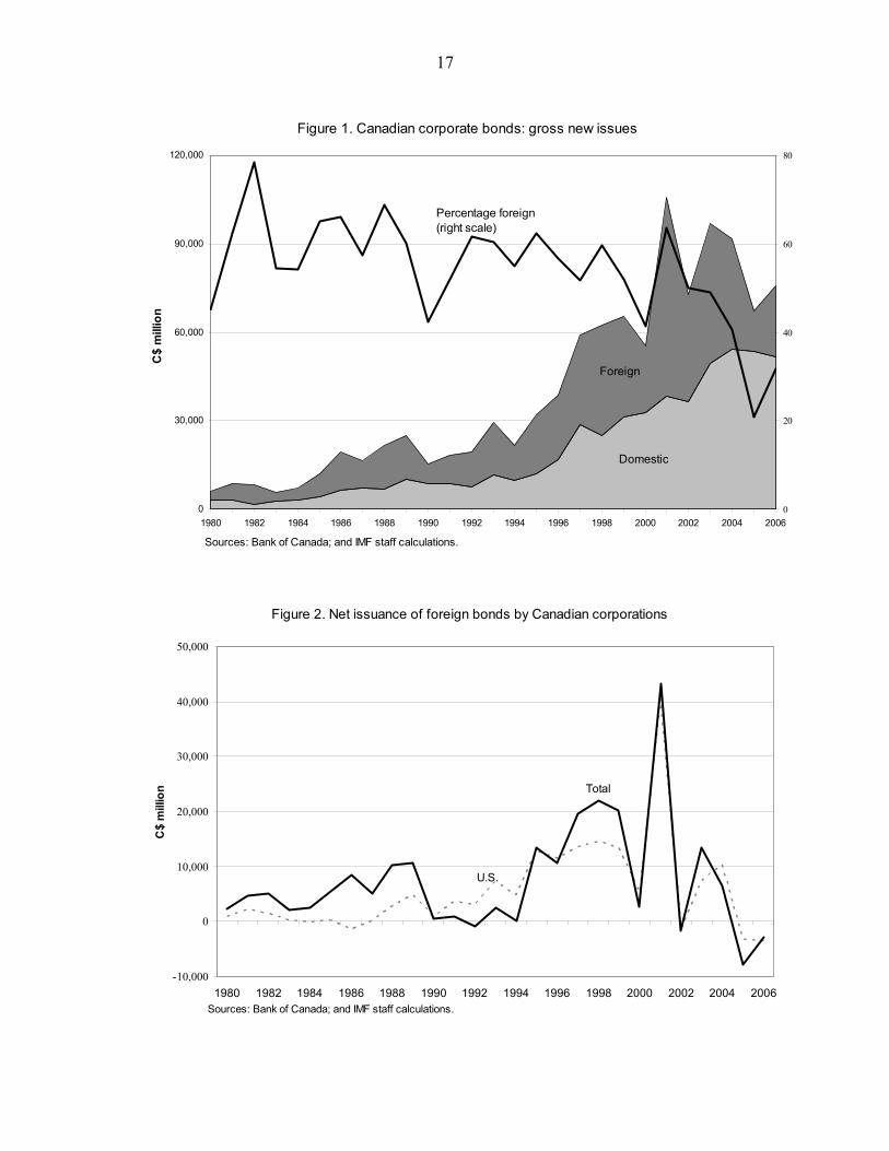
II. FINANCIAL LINKAGES

Given the close geographic proximity, the extent of financial flows between Canada and the United States is hardly surprising. The stock of U.S. claims on Canadian assets equaled 53 percent of Canada’s GDP at the end of 2006. The commonalities of language, culture, and business environment, as well as openness to trade in goods, services, and assets facilitate cross-border flows of capital. In addition, the size and sophistication of U.S. financial markets make them an attractive source of capital, as they may offer features and liquidity not available in Canada.2 In Canada, banks are the main source of short-term corporate credit, while long-term financing is dominated by equity (38 percent of long-term corporate credit outstanding at the end of 2006) and bond financing (34 percent), with the rest accounted for by trust units,3 rapidly growing securitization, and other vehicles. The extent of reliance of Canadian non-financial corporations on U.S. financing is documented in Freedman and Engert (2003), who show that in the early 2000s just under 40 percent of outstanding Canadian corporate bonds were issued in the United States,4 while the share of foreign (primarily U.S.) placement of new Canadian stocks was around 20–25 percent. More recent data confirm these findings. Figure 1 shows that in the 2000s Canadian corporations relied on foreign markets for 20 to 60 percent of their bond issuance. Of course, “foreign” does not necessarily mean “U.S.,” but it is a received wisdom that for Canada it largely does—the fact that is confirmed by a close correspondence between the net issuance of U.S. and all foreign bonds by Canadian corporations,5 particularly since the mid-1990s (Figure 2). The percentage of Canadian stocks held by U.S. residents has stayed between 15 and 20 percent in recent years (Figure 3). According to BIS data, foreign loans account for 20 to 40 percent of total bank loans to the Canadian non-bank sector, depending on whether mortgage lending is included or excluded (Figure 4), although the share of U.S. banks in that number is not clear. All in all, it appears that about one quarter of financing is raised by Canadian corporations south of the border. This sizable dependence on U.S. funding sources gives rise to the vulnerability of Canada’s real economy to changes in U.S. financial conditions. Canadian firms and households

2 For example, the market for high-yield bonds is virtually non-existent in Canada (Calmès, 2004).

3 Income trusts are flow-through entities that became popular in Canada in the late 1990s and particularly early this decade due to their tax advantages. A series of recent government measures have sought to eliminate these advantages, halting further expansion of that sector.

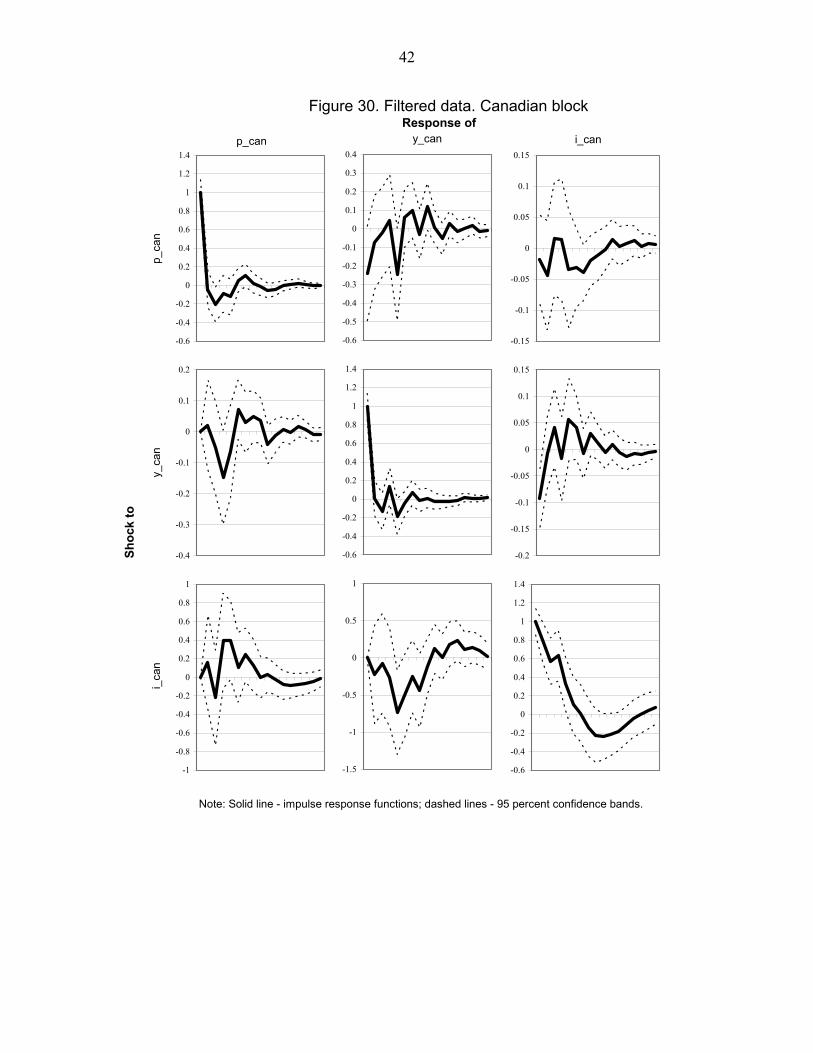
4 The fraction of Euro-dollar bonds varied between 5 and 9 percent, and the share of other non-Canadian bonds was negligible.

5 A breakdown by country for gross issuance of foreign bonds is not available.

6

may also be exposed to U.S. financial conditions through their holdings of U.S. assets, which have increased in recent years.6

III. MODEL

Given the extent of financial linkages between Canada and the United States, the idea that tighter financial conditions in the latter would temper output growth in the former does not appear controversial. Still, we use a simple model to illustrate the effect and to help introduce certain concepts. In the model, Canadian firms use capital K to produce output with a diminishing marginal product of capital (MPK). Capital depreciates fully in one period. To produce, the firms need to purchase capital using borrowed funds D. Some firms can borrow only domestically, while others have access to the U.S. capital market. The interest rate on funds raised in either market increases in the amount borrowed. We will assume that the rate for domestic borrowing is initially lower than for foreign borrowing, reflecting the cost of accessing the foreign market; but it rises faster with growing domestic indebtedness, due to the smaller size and liquidity compared to the U.S. market. We abstract from exchange rate issues.7 The model is admittedly very simple, but it captures the conventional channel through which financial conditions affect the real economy. The demand and supply curves for funds are drawn in Figure 5. The former is simply the MPK curve. The latter combines the domestic and foreign interest rate schedules as functions of borrowing. As discussed above, the Canadian schedule starts lower but is steeper than the U.S. schedule, so up to the point where the two curves intersect, Canadian companies would borrow domestically. Beyond that, the Canadian firms that have access to U.S. funds will diversify their borrowing, and the effective interest rate schedule will run between the domestic and foreign ones. The intersection of the combined interest rate schedule and the MPK line will give the total amount borrowed and hence the total capital installed. This, in turn, will determine the amount of output produced. If the U.S. interest rate schedule shifts up, representing a tightening of financial conditions in that country, the effective Canadian schedule will shift up as well (Figure 6). As a result, Canadian firms will borrow less, lowering their capital intensity and production.8 We call the resulting reduction in output the direct effect.

6 For example, the stock of portfolio investment in U.S. assets by Canadian residents stood at 13 percent of GDP at the end of 2006.

7 One could think of these interest rate schedules as corrected for expected exchange rate movements; the schedules would not coincide given that domestic and foreign borrowing are not perfect substitutes.

8 Even though capital does not depreciate as fast as our model assumes, and not all capital purchases have to be financed by external funds, there is little doubt that tighter financial conditions hamper output growth by making working capital more expensive and by crimping investment (as well as lowering household consumption through the wealth effect and tighter credit).

7

If the Canadian interest rate schedule also shifts up in response to a tightening of financial conditions in the United States, there will be an additional, indirect effect on output, stemming from higher cost of domestic finance (Figure 7). Financial conditions in Canada may be affected by financial conditions in the United States both through the demand channel (with U.S. funding more expensive, more borrowers would switch to the Canadian market, bidding up the interest rate there) and the supply channel (cost of raising funds for financial institutions will go up, and they will pass that increase to their borrowers). Confidence effects may also play a role. The relative size of the direct and indirect effects depends on the relative steepness of the Canadian and U.S. interest rate schedules and on the magnitude of the response of the former to the shift in the latter. As long as our assumptions about access to and depth of the markets hold (so that the U.S. schedule intersects the Canadian one from above, and thus the United States is the marginal lender) and the reaction of the Canadian schedule to a shift in the U.S. schedule is no greater than one for one, the direct effect will be larger.

IV. EMPIRICAL ANALYSIS

We now proceed to examine empirically the links between financial conditions in the United States and real activity in Canada. We start by running a simple six-variable structural vector autoregression (SVAR) that includes the CPI inflation rate, the real GDP growth rate, and the 3-month Treasury bill rate for each country. The interest rate is our measure of financial conditions. The growth rate and the inflation rate are the measures of economic activity that both affect (including through the monetary policy reaction function) and are affected by the interest rate. Given the relative economic size of the two countries, we assume that Canadian variables do not have an effect on U.S. variables, either simultaneously or with lags. This block exogeneity (Hamilton, 1994, p.309) assumption, similar to the approach taken by Cushman and Zha (1997) and by Dungey and Pagan (2000), reduces the number of parameters that require estimation and thus allows more precise estimates. Within each block, we make the standard assumption of the following ordering of the variables: inflation, real growth, and the interest rate. Inflation is the most inertial variable. The interest rate, as a financial variable, is the most fast-moving one. It reflects, among other things, monetary policy or anticipation thereof, based (at least in part) on growth and inflation. Given the lags in monetary policy transmission, the interest rate reacts faster to the shocks to output and inflation than they react to changes in the interest rate. This ordering is quite popular in the literature, although by no means is it unique or without critics.9 In terms of cross-linkages, we allow U.S. variables to have a simultaneous impact on corresponding Canadian variables as well as on the Canadian variables that come later in the ordering. So, for example, a shock to the U.S. real GDP growth will simultaneously affect the U.S. interest rate, Canada’s real GDP growth, and Canada’s interest rate. There are no restrictions on the impact of lagged U.S. variables on U.S. or Canadian variables. 9 See Christiano and others (1999) for a discussion of various identification schemes.

8

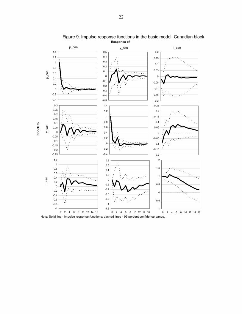
We use quarterly data from the first quarter of 1983 through the first quarter of 2007, aiming to have as many observations as possible, but confining our sample to the epoch of the “great moderation” (Stock and Watson, 2002), since the macroeconomic environment was quite different in the preceding period. Inflation and output growth are annualized quarterly growth rates of seasonally adjusted CPI and real GDP series. With quarterly data, four is a natural choice for the number of lags in the VAR.10 The impulse response functions for the estimated system are exhibited in Figures 8–10. The solid lines represent impulse responses, and the dashed lines confine analytically constructed 95-percent confidence bands.11 The magnitude of a shock is one unit of the corresponding variable, i.e. one percentage point. The responses are calculated for 16 quarters. Figure 8 shows the responses of U.S. variables to U.S. shocks. The picture looks quite familiar. A shock to the inflation rate leads to a spike in inflation, a drop in output, and higher interest rates. A shock to GDP growth pushes inflation, output growth, and interest rates up. A spike in the interest rate is quite persistent, and leads over time to lower output growth. The only perverse response is a rise in inflation in reaction to a positive interest rate surprise, but this price puzzle is by no means unique to this paper. All in all, this set of impulse responses conforms with our priors and gives us fair confidence that U.S. shocks are identified reasonably well. Responses of Canadian variables to Canadian shocks are found in Figure 9. Inflation shows less persistence than in the United States, and the impact of inflation shocks on output growth and the interest rate is small. The magnitude of inflation and interest rate responses to output shocks is also insignificant. This may reflect the open character of the Canadian economy—domestic shocks play a relatively minor role. The price puzzle is present, but much less pronounced than in the United States. The output response to changes in the interest rate appears somewhat more sluggish. Finally, Figure 10—the focus of our attention—presents the responses of Canadian variables to U.S. shocks.12 Confirming the conventional wisdom, we find a strong response of Canada’s real GDP to a shock to the U.S. GDP growth (the middle pane), with a change in Canada’s growth peaking at about one half of the U.S. impulse. We can also see that tighter financial conditions in the United States tend to lead to tighter financial conditions in Canada (bottom right pane), in line with anecdotal evidence. An increase in the U.S. interest rate leads to an approximately equal rise in the Canadian rate. This does not mean that the Bank of Canada follows the stance of the Federal Reserve irrespective of the cyclical positions of the two economies—the interest rate shock in our system is orthogonal to the systematic response of monetary policy to 10 The results for the six-variable model were very similar when only three lags were used.

11 Confidence bands constructed using parametric bootstrap are virtually indistinguishable from analytical ones. The results are available upon request.

12 Under the block exogeneity assumption, the responses of U.S. variables to shocks emanating from Canada are nil.

9

fluctuations in output and inflation. A key finding, which we probe deeper in the next section, is the fact that a tightening of financial conditions in the United States leads to a statistically significant reduction in real GDP growth in Canada (bottom middle pane). Variance decomposition (Figure 11) demonstrates that foreign shocks are an important source of variation in Canada’s real GDP growth, accounting for over 40 percent of forecast error variance at horizons longer than a year. Within that group, shocks to U.S. output growth are the most significant. “Nonsystematic” interest rate volatility—changes that are not identified as responses to demand or supply shocks and hence captured as interest rate shocks in the econometric model—was quite low in the sample period,13 and U.S. interest rate shocks account for slightly over 5 percent of the forecast error variance for Canada’s real GDP growth at horizons over one year. At the same time, as our results indicate, a large financial shock in the United States would have a substantial impact on the Canadian economy.

V. TRANSMISSION OF U.S. FINANCIAL SHOCKS TO CANADA

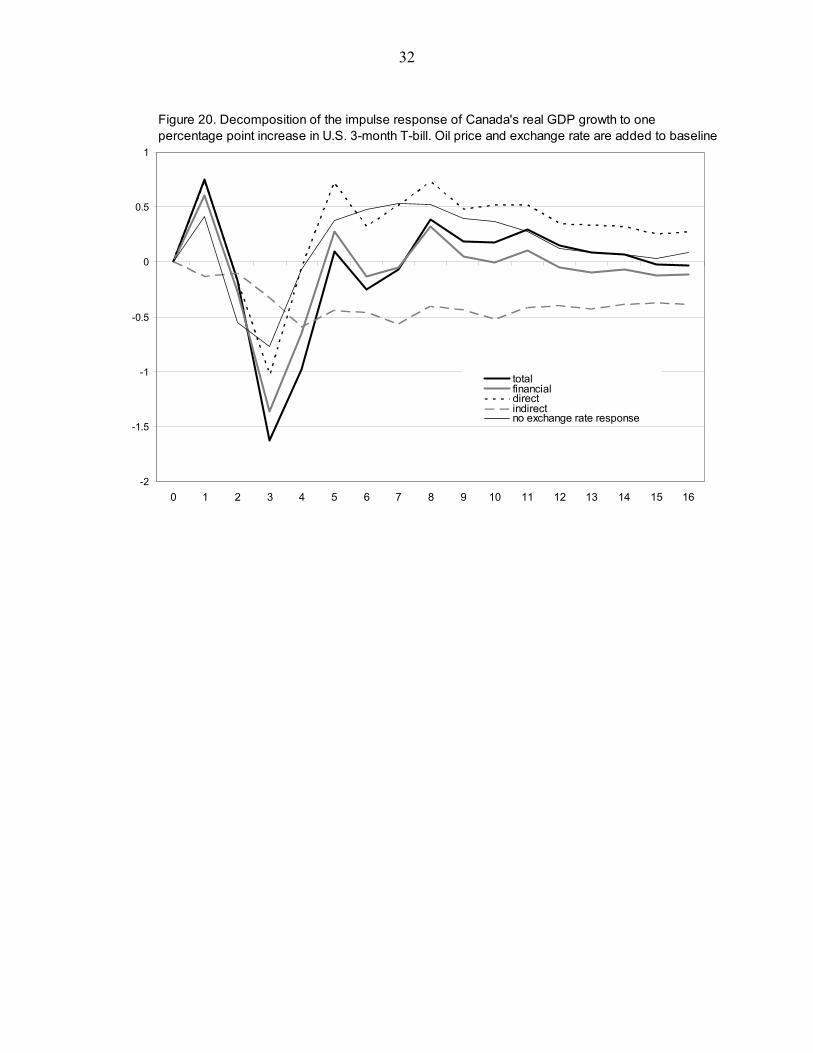
As discussed above, the negative response of the Canadian real GDP growth to an increase in the U.S. interest rate may come through one of three channels. First, tighter financial conditions in the United States lead to lower growth in the United States (see Figure 8, bottom middle pane), which would then lead to lower demand for Canadian exports and hence lower growth in Canada (Figure 10, middle pane). We call this the trade channel. Second, higher interest rates in the United States tend to lead to higher interest rates in Canada (Figure 10, bottom right), which in turn will dampen output (Figure 9, bottom middle). We call this the indirect financial channel. Finally, the direct financial channel would primarily reflect a reduction in investment and production by Canadian firms using U.S. financing and represent a slowdown in Canada that is not ascribed to lower U.S. growth or higher Canadian interest rates. Figure 12 presents the decomposition. The thick solid black line is the total response of Canada’s growth to a one percentage point shock to the U.S. interest rate—same as in the bottom middle pane of Figure 10. To isolate the financial channels, we shut down the trade channel by setting to zero the coefficients of Canadian variables on contemporaneous and lagged U.S. growth in the SVAR.14 The result is shown by the thick solid gray line. We can observe that the bulk of the impact of higher U.S. interest rates on Canadian growth, particularly in the short run, comes through the financial rather than trade channel.

13 While the standard deviations of the U.S. interest rates and real GDP growth rates were very close in the sample period (2.3 percentage points and 2.2 percentage points, respectively), the standard deviation of the shocks to the U.S. interest rate was estimated at 0.3 percentage point—quite a bit lower than 1.8 percentage points for U.S. real GDP growth.

14 Shutting down the trade channel by setting the coefficients of only Canada’s GDP growth on U.S. growth to zero or by holding U.S. growth constant yields nearly identical results.

10

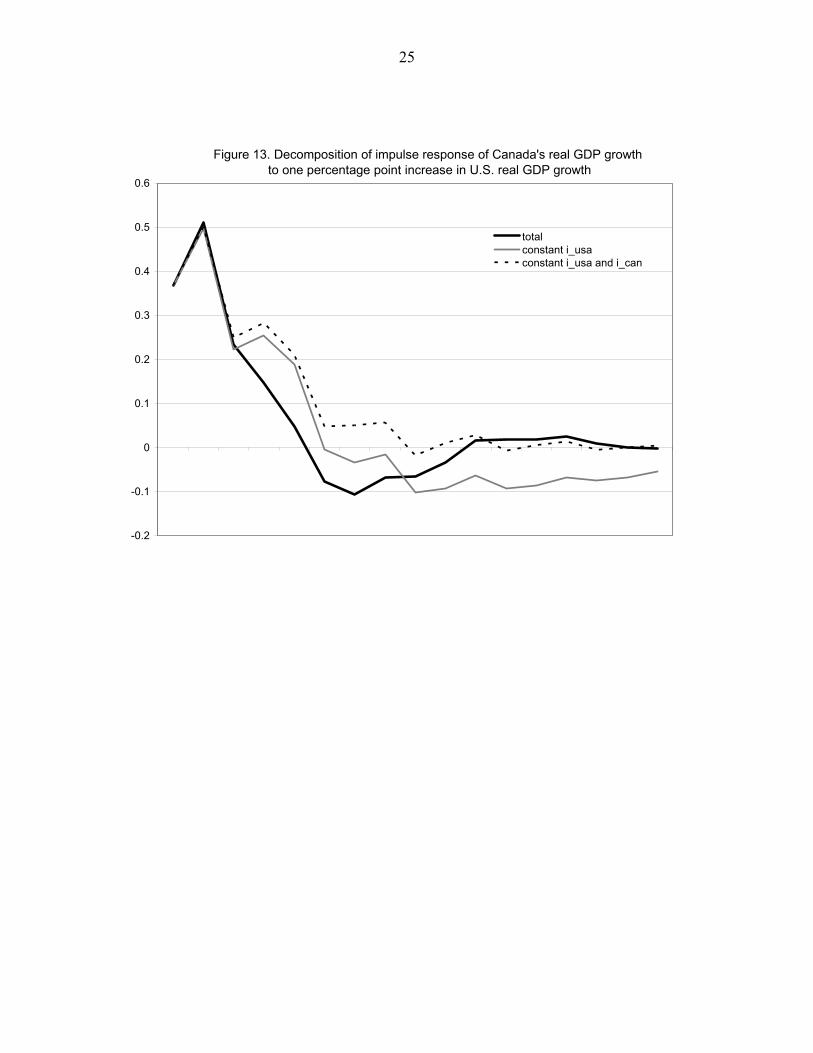
To isolate the direct financial channel (the dotted black line), we shut down the indirect channel by holding the Canadian interest rate constant.15 The indirect channel (the dashed gray line) is then obtained as a residual. The direct channel accounts for most of the short-run decline in output growth. In the medium term the response switches to the other side. The way we interpret this is that facing constant U.S. demand and unchanged Canadian interest rates, but higher U.S. interest rates (that is the experiment captured in the direct financial channel), Canadian firms that rely primarily on the United States for their funding initially reduce their output and investment; later, however, they can switch to alternative sources of finance (domestic credit or retained earnings) and make up some of the lost ground. The indirect channel is relatively small, but quite persistent, keeping growth near the trend in the medium term by offsetting the rebound in the direct channel. We conclude that U.S. financial conditions are quite important for Canada—a one percentage point increase in the short-term interest rate in the United States leads to a decline in real GDP growth in Canada of up to 1¼ percentage points. The impact is largely fed through the financial channel, in the first instance affecting the firms relying on U.S. funding, and with more lingering effects through tightening financial conditions in Canada. As an aside, we conduct a decomposition of the impact on Canada’s real GDP of a shock to U.S. real GDP growth. Such a shock would be counteracted by both U.S. and Canadian monetary policy, dampening its effect on Canada. As Figure 13 demonstrates, holding the U.S. interest rate constant would make the effect of the U.S. demand shock more persistent, removing the stabilizing influence of monetary policy at the 3-4 quarter horizon. The effect is rather minor. Shutting down the Canadian interest rate response on top of that produces a small additional correction.

VI. SENSITIVITY ANALYSIS AND EXTENSIONS

Including the oil price The oil price is an important driver of inflation in both countries and can also affect output. It has been suggested (e.g., Sims, 1992) that including oil prices in VARs can improve the identification of monetary shocks. Figures 14-16 show impulse responses with the annualized quarterly growth rate of the West Texas Intermediate (WTI) price included in the regressions. It is placed in the U.S. block, first in the ordering, and assumed to be able to affect simultaneously all Canadian variables as well as all U.S. variables, and not to be affected by Canadian variables. The inclusion of oil prices does not change substantially the impulse responses of the other variables. It does reduce the magnitude of the price puzzle (an upward jump in inflation in response to a positive interest rate shock) by almost a half, but does not eliminate it completely.

15 Disallowing only the response of Canada’s interest rate to the U.S. interest rate results in a virtually identical decomposition.

11

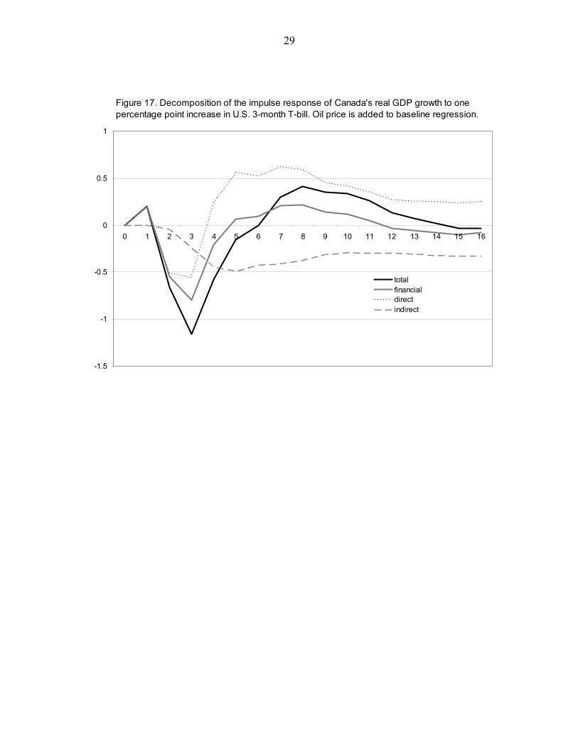
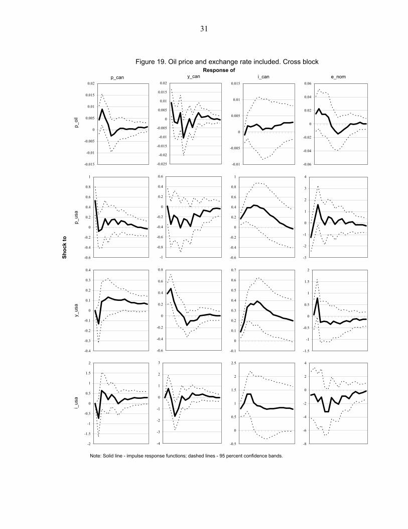
As expected, a positive demand shock in the United States pushes oil prices up. Higher oil prices lead to higher inflation and interest rates in both the United States and Canada.16 They also push down real GDP growth in the United States, while the impact on Canada is close to zero on average, reflecting Canada’s endowment in hydrocarbon resources. The profile, magnitude, and decomposition of the impulse response of Canada’s GDP growth to a one percentage point shock to the U.S. interest rate is very similar to the case without oil (Figure 17). Including oil and the exchange rate If the U.S. interest rate goes up, and is not followed by the Canadian rate (the mental experiment we use to define the direct financial channel), the Canadian dollar will likely depreciate against the U.S. dollar. This, in turn, would stimulate Canada’s GDP by boosting net exports. That mechanism may partly offset the direct financial effect and lead to its underestimation. To check the importance of that mechanism, we run a SVAR that includes the nominal Canada-U.S. exchange rate (defined as the price of the Canadian dollar in U.S. dollars, so that an increase means appreciation). The annualized quarterly change of the exchange rate is placed last in the Canadian block on the assumption that it is the fastest-moving variable. We also include the oil price, which is a major determinant of the strength of the Canadian dollar (Issa and others, 2006) in this system (first in the U.S. block). The impulse responses involving the exchange rate look largely as expected (Figures18-19)17. The Canadian dollar appreciates after a shock to the Canadian interest rate (although after an initial drop) and after positive shocks to output or inflation (probably reflecting expectations of tighter monetary policy is response). It also appreciates in response to a rise in oil prices, which is a terms-of-trade improvement for Canada. A shock to the U.S. interest rate leads to a depreciation of the Canadian dollar. A positive shock to the exchange rate (an appreciation) leads on average to a slight decrease in Canada’s interest rate (consistent with the Bank of Canada policy of counteracting exchange rate movements not caused by changes in the demand for Canadian goods and services) and depresses Canadian output. Perversely, inflation appears to pick up in Canada in response to currency appreciation—another manifestation of the price puzzle. To net out the exchange rate effect, we reproduce the impulse response function of Canadian output growth to the U.S. interest rate holding the exchange rate constant. As Figure 20 16 The effect on Canada is smaller, probably due to higher gasoline taxes in that country and the tendency of its currency to appreciate on higher oil prices.

17 The impulse response functions in the U.S. block look nearly identical to those in Figure 14, and hence are not shown. Since the coefficients are estimated using a system method, the composition of the Canadian block affects the estimates for the U.S. block, which explains the small differences. Full results for this and other specifications are available upon request.

12

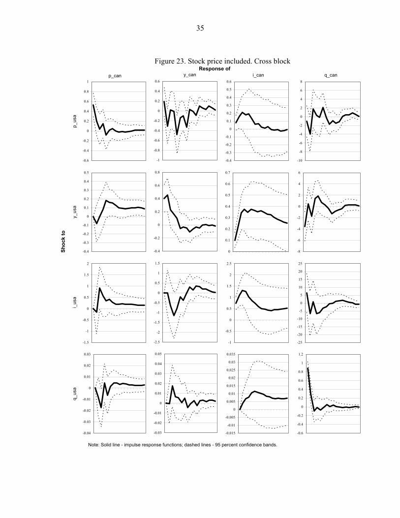
demonstrates, the effect is hardly discernible—fixing the exchange rate barely affects the location of the line showing the propagation of the interest rate shock via the direct channel. Including stock prices Borrowing is not the only way to raise capital. We extend our baseline regression by including the growth rates of stock price indices for the United States and Canada (S&P500 and TSX/SP300, respectively). We put the stock indices last in each country’s block, assuming they are the most reactive variables.18 The impulse response functions of this eight variable SVAR are presented in Figures 21-23. In the United States, stock prices go down on inflationary surprises, but do not appear to react strongly to output or interest rate. A jump in stock prices pushes up the interest rate and predicts higher output growth and, after about three quarters, inflation. In Canada, stocks exhibit a pronounced negative response to higher interest rates and a pronounced positive response to higher output. They also appear to go up, after about a year’s delay, on inflation. One could speculate that the concurrence of higher inflation and higher stock prices may reflect a heavy representation of energy companies in Canada’s stock market, although the timing of the response makes this rationalization not very probable. Higher output follows a positive stock market surprise, while the response of the interest rate and inflation is small. Finally, Figure 23 confirms the extent of real and financial linkages between the United States and Canada. Higher output growth in the United States leads to higher output growth in Canada. Canadian stocks go up when U.S. stocks go up (and nearly as much), and Canadian interest rates rise in response to higher U.S. interest rates. Regarding the importance of U.S. financial conditions for Canada’s real economy, we note, as before, that a shock to U.S. interest rates pushes Canadian GDP growth rate down; and we can also see that higher stock prices in the United States, which imply easier financial conditions, lead to higher output growth in Canada. Including spreads on long-term corporate bonds As a complementary measure of financial conditions we include the spreads of U.S. and Canadian corporate long-term bond yields over corresponding 10-year Treasury rates. As can be seen from Figure 24, wider corporate spreads in the United States appear to have a negative impact on Canadian GDP growth, although the results are not statistically significant. Wider U.S. spreads also trigger wider spreads in Canada. The impact of higher 3-month T-bill rate on Canadian real GDP growth, interest rate and inflation in this specification is close to that in the baseline. Including financial conditions indices 18 The forward-looking nature of financial variables complicates identification, and evidence drawn from VARs that include stock prices should be interpreted cautiously. See Sellin (2001) for an informative survey.

13

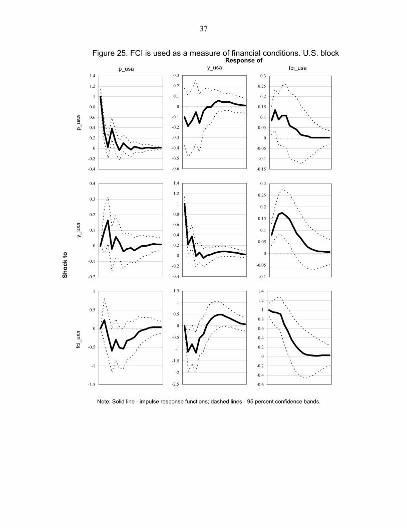
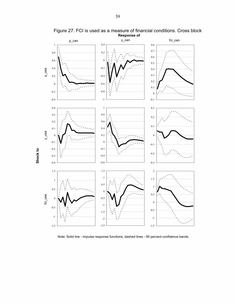
Obviously our baseline measure of financial conditions—the yield on the three-month Treasury bill—does not capture those conditions fully. Adding other asset prices to the baseline specification one by one alleviates that concern only partially, as it still leaves many potentially useful variables out. The problem should not be exaggerated, as various asset prices tend to be highly correlated. Still, a more encompassing and at the same time parsimonious approach would be to use a single, comprehensive measure of financial conditions. Fortunately, researchers at both central banks and private sector institutions have been working on developing such measures, called financial conditions indices (FCI), and using them for some time. Unfortunately, the task of capturing financial conditions in one index is quite complex and can be solved only imperfectly, and both construction and use of FCI has been subject to numerous criticisms. Gauthier and others (2004) provide a comprehensive survey and suggest several new FCIs for Canada. Incidentally, they find that FCIs that use U.S. stock prices and high-yield bond spreads are better predictors of Canadian output than indices that include Canadian financial variables—a result consistent with the main theme of this paper. Recognizing the weaknesses, we include FCIs in a robustness check rather than in our baseline regression. The indices we use are similar to the Goldman Sachs FCI for Canada and the United States.19 Both indices include measures of real short-term market interest rates, real exchange rate, and equity valuation. The U.S. index also incorporates the real yield on long-term corporate bonds, while the Canadian index adds the slope of the yield curve. Higher values represent tighter financial conditions. The construction of the indices is discussed in the Appendix. The impulse response functions from the specification that includes the FCIs are reproduced in Figures 25–27. The results are largely similar to those in the baseline, but a few differences emerge, particularly in the U.S. block (Figure 25). For one, the price puzzle disappears—tighter financial conditions are associated with lower inflation. Second, the output responds more sharply to a tightening in the FCI than to an increase in the 3-month rate. This is not surprising, given that FCIs are explicitly designed not only to reflect current financial conditions, but also to be able to predict GDP growth at short horizons (Dudley and Hatzius, 2000). Third, the responses of the FCI to inflation and output shocks is more front-loaded and less persistent than those of the interest rate, and shocks to the FCI itself also induce less persistent movements in the index than is the case for the interest rate. Similar observations can be made about the Canadian block (Figure 26). Notably, inflation surprises elicit a sharp tightening of financial conditions as measured by the FCI. At the same time, a positive shock to output appears to loosen financial conditions. This may reflect our ordering assumption, where comovements between real GDP growth and the FCI are attributed to growth moving first and the FCI reacting. If, in fact, looser financial conditions can stimulate

19 The main reason to use the Goldman Sachs indices was the presumption that indices constructed by the same institution would be more compatible, and in the Gauthier and others (2004) review Goldman Sachs was the only institution that had FCI both for the United States and for Canada.

14

real GDP growth within the quarter, this correlation would be misinterpreted in our identification scheme. This simultaneity problem may be more severe for the FCI than for the interest rate if stock prices and exchange rates (variables included in the FCI) are more forward-looking than the short-term interest rate and if the economy reacts faster to them. Both conditions may well be true. Finally, in the cross block (Figure 27) we still observe that a tightening of financial conditions in the United States leads to a substantial decline of real GDP growth in Canada, which lasts about two years. Tighter financial conditions in the United States also lead to tighter financial conditions in Canada (although with less persistence than for interest rates), and GDP growth surprises in the United States move Canadian growth in the same direction and with about half the magnitude. In the forecast error variance decomposition, shocks to U.S. financial conditions account for 6–8 percent of variance in Canada’s real GDP growth at the 6–16 quarter horizons, compared to the 5 percent share of U.S. interest rate shocks. While these results are broadly similar to our baseline, the decomposition of the impact of the U.S. financial shock on the Canadian output is not. As can be seen from Figure 28, when the U.S. real GDP growth is held constant, Canadian growth does not appear to respond in a coherent fashion to U.S. financial conditions, but rather oscillates wildly around the zero line. Averaging these fluctuations out, one would conclude on the basis of that picture that the financial transmission channel does not work, and all the impact of tighter U.S. financial conditions on Canada comes through slower growth in the United States. A further decomposition shows that the indirect channel behaves in the expected way, but the direct channel exhibits a perverse swing, with growth accelerating in Canada if financial conditions tighten in the United States but not north of the border. One could rationalize that by noting the forward-lookedness of financial variables included in the FCI. Divergence between U.S. and Canadian FCIs, on which this exercise is predicated, could arise if there were bad news for U.S. growth and good news for Canadian growth, which would be incorporated into the respective FCIs, for example, via stock prices. In addition, given the FCI’s intended use as a predictor of GDP growth several quarters ahead, its composition may be biased in a way that overstates the impact of domestic financial conditions on GDP growth, hence exaggerating the significance of the trade channel in our decomposition. To summarize, taken at face value, SVARs with the FCIs instead of the interest rates confirm the importance of U.S. financial conditions for growth and financial conditions in Canada, but do not confirm the importance of the direct financial channel in the transmission of U.S. shocks to Canada. However, given the uncertainties involved in constructing financial condition indices, both the confirmation and the rejection should be regarded with a dose of skepticism. Filtering data One may be concerned that the degree of cyclical interdependence in our regressions may be exaggerated if Canada and the United States followed similar long-term trends—such as

15

common productivity shocks or simultaneous disinflations. To address these concerns, we detrend the data using HP filter20 and apply our SVAR to detrended data. The impulse response functions from this SVAR look similar to those obtained on raw data (Figures 29–31). The price puzzle appears smaller in the detrended data, and the interest rate shocks are less persistent. The response of the Canadian output to a shock to the U.S. output is a bit smaller in the short run and changes sign in the medium run. The decline of Canada’s real GDP growth in response to a tightening in U.S. financial conditions remains large and statistically significant. The share of U.S. interest rate shocks in the variance decomposition of Canada’s real GDP growth rises to 10 percent in this specification. It should be noted, however, that with detrending the size of the direct financial channel decreases, while that of the indirect financial channel rises substantially (Figure 32). Changing time period Since the monetary regime was changed in Canada in February 1991 with the introduction of inflation targeting (IT), we rerun the baseline SVAR on the period 1991Q1-2007Q1. The impulse response functions are shown in Figures 33–35. Qualitatively the picture looks similar to that obtained over the longer period. However, with the shorter sample and less variability, the shocks and responses are more difficult to identify, and the confidence bands are wider. The response of Canadian growth to U.S. interest rates is somewhat smaller, but more protracted. The decomposition (Figure 36) looks similar to that over the full period, although the direct effect appears smaller. The response of Canadian GDP growth and interest rates to corresponding U.S. variables is also a bit smaller, and the interest rate reaction is also noticeably less persistent. Canadian interest rates appear to go down rather than up in response to an inflation shock in the United States. We have too few degrees of freedom to make conclusive comparisons between the inflation targeting and the pre-IT periods, but our results are consistent with the notion that Canada has become somewhat less dependent on the United States in the last decade.

VII. CONCLUSION

In this paper we have established that in addition to substantial trade linkages, Canada and the United States are connected through financial markets. Canadian corporations raise about one quarter of their financing south of the border, with bonds playing a particularly important role. As a result, financial conditions in the United States have substantial influence over both financial conditions and real economic activity in Canada.

20 Specifically, we apply the HP filter with a smoothing parameter of 1600 to the logs of CPI and real GDP and to the interest rates. The growth rates of the cycle components of CPI and GDP and the cycle component of the interest rates then enter the regression.

16

Using a SVAR approach, we have confirmed that shocks to U.S. real GDP growth have a considerable impact on Canadian GDP growth, with the coefficient of about one half. We have also found that financial shocks are transferred almost one-for-one from the United States to Canada. Finally, a tightening of financial conditions in the United States leads to a statistically and economically significant slowdown in Canada’s real GDP growth. The direct financial channel, affecting Canadian firms raising funds in the United States, is particularly important in the short run. The indirect financial channel, where the impact on real activity is fed through the influence of U.S. financial conditions on those in Canada, exhibits smaller magnitude, but more persistence. The finding that U.S. financial shocks have a major impact on financial conditions and real GDP growth in Canada, and, to a somewhat lesser extent, the decomposition of the latter effect, are robust to a number of specification changes, with various measures of U.S. financial conditions affecting financial conditions and real activity in Canada. These results imply that a substantial financial shock emanating from the United States—like the one we are witnessing now—may have severe implications for the Canadian economy. Despite tentative indications that Canada has become somewhat less dependent on its southern neighbor in the recent period, the extent of both real and financial linkages between the two countries remains large, and their interplay creates a transmission mechanism for foreign shocks that should not be overlooked.

17

Figure 1. Canadian corporate bonds: gross new issues

0

30,000

60,000

90,000

120,000

1980 1982 1984 1986 1988 1990 1992 1994 1996 1998 2000 2002 2004 20060

20

40

60

80C

$ m

illio

n

Domestic

Foreign

Percentage foreign (right scale)

Sources: Bank of Canada; and IMF staff calculations.

-10,000

0

10,000

20,000

30,000

40,000

50,000

1980 1982 1984 1986 1988 1990 1992 1994 1996 1998 2000 2002 2004 2006

C$

mill

ion Total

U.S.

Sources: Bank of Canada; and IMF staff calculations.

Figure 2. Net issuance of foreign bonds by Canadian corporations

18

0

5

10

15

20

25

30Q

1-19

90

Q4-

1990

Q3-

1991

Q2-

1992

Q1-

1993

Q4-

1993

Q3-

1994

Q2-

1995

Q1-

1996

Q4-

1996

Q3-

1997

Q2-

1998

Q1-

1999

Q4-

1999

Q3-

2000

Q2-

2001

Q1-

2002

Q4-

2002

Q3-

2003

Q2-

2004

Q1-

2005

Q4-

2005

Q3-

2006

Sources: Haver Analytics; and IMF Staff calculations.

Figure 3. Percentage of shares of Canadian companies held by U.S. residents

0

10

20

30

40

50

Dec

-95

Jun-

96

Dec

-96

Jun-

97

Dec

-97

Jun-

98

Dec

-98

Jun-

99

Dec

-99

Jun-

00

Dec

-00

Jun-

01

Dec

-01

Jun-

02

Dec

-02

Jun-

03

Dec

-03

Jun-

04

Dec

-04

Jun-

05

Dec

-05

Jun-

06

Dec

-06

Excluding mortgages

Including mortgages

Sources: Bank of Canada; Bank for International Settlements; and IMF staff calculations.

Figure 4. Foreign loans to Canadian non-bank sector as percentage of bank loans to Canadian non-financial corporations

19

i

KD

MPK

i can

i us

i combined

Figure 5. Determination of capital level

i

K

MPK

i can

i us

i combined

Direct effect

Figure 6. Direct impact of tightening in U.S. financial conditions

i combined'

i us'

20

i

K

MPK

i can

i us

i combined

Indirect effect

Figure 7. Indirect impact of tightening in U.S. financial conditions

i combined''

i us'

i can''

i combined'

21

Figure 8. Impulse response functions in the basic model. U.S. block

Note: Solid line - impulse response functions; dashed lines - 95 percent confidence bands.

-0.4

-0.2

0

0.2

0.4

0.6

0.8

1

1.2

1.4

-0.6

-0.5

-0.4

-0.3

-0.2

-0.1

0

0.1

0.2

0.3

-0.3

-0.2

-0.1

0

0.1

0.2

0.3

0.4

-0.2

-0.1

0

0.1

0.2

0.3

0.4

-0.4

-0.2

0

0.2

0.4

0.6

0.8

1

1.2

1.4

0

0.05

0.1

0.15

0.2

0.25

0.3

0.35

0.4

0.45

-0.6

-0.4

-0.2

0

0.2

0.4

0.6

0.8

1

1.2

1.4

1.6

0 2 4 6 8 10 12 14 16-2

-1.5

-1

-0.5

0

0.5

1

1.5

0 2 4 6 8 10 12 14 16-0.2

0

0.2

0.4

0.6

0.8

1

1.2

1.4

1.6

1.8

2

0 2 4 6 8 10 12 14 16

p_usa y_usa i_usay_

usa

i_us

ap_

usa

Shoc

k to

Response of

22

Figure 9. Impulse response functions in the basic model. Canadian block

-0.4

-0.2

0

0.2

0.4

0.6

0.8

1

1.2

1.4

-0.5

-0.4

-0.3

-0.2

-0.1

0

0.1

0.2

0.3

0.4

0.5

-0.2

-0.15

-0.1

-0.05

0

0.05

0.1

0.15

0.2

-0.25

-0.2

-0.15

-0.1

-0.05

0

0.05

0.1

0.15

0.2

0.25

0.3

-0.4

-0.2

0

0.2

0.4

0.6

0.8

1

1.2

1.4

-0.2

-0.15

-0.1

-0.05

0

0.05

0.1

0.15

0.2

0.25

-1

-0.8

-0.6

-0.4

-0.2

0

0.2

0.4

0.6

0.8

1

1.2

0 2 4 6 8 10 12 14 16-1.2

-1

-0.8

-0.6

-0.4

-0.2

0

0.2

0.4

0.6

0.8

0 2 4 6 8 10 12 14 16-1

-0.5

0

0.5

1

1.5

2

0 2 4 6 8 10 12 14 16


Response ofSh

ock

to

p_can y_can i_canp_

can

y_ca

ni_

can

23

Figure 10. Impulse response functions in the basic model. Cross block

-0.6

-0.4

-0.2

0

0.2

0.4

0.6

0.8

1

-1

-0.8

-0.6

-0.4

-0.2

0

0.2

0.4

0.6

-0.4

-0.3

-0.2

-0.1

0

0.1

0.2

0.3

0.4

0.5

0.6

-0.4

-0.3

-0.2

-0.1

0

0.1

0.2

0.3

0.4

-0.4

-0.2

0

0.2

0.4

0.6

0.8

1

-0.1

0

0.1

0.2

0.3

0.4

0.5

0.6

0.7

-1.5

-1

-0.5

0

0.5

1

1.5

2

2.5

0 2 4 6 8 10 12 14 16-3

-2.5

-2

-1.5

-1

-0.5

0

0.5

1

1.5

0 2 4 6 8 10 12 14 16-1

-0.5

0

0.5

1

1.5

2

2.5

0 2 4 6 8 10 12 14 16


Response ofSh

ock

to

p_can y_can i_canp_

usa

y_us

ai_

usa

24

Figure 11. Shares of forecast error variance of Canada's real GDP growth due to differenet shocks

0

0.1

0.2

0.3

0.4

0.5

0.6

0.7

0.8

0.9

1

1 2 3 4 5 6 7 8 9 10 11 12 13 14 15 16

i_can

y_can

p_can

i_usa

y_usa

p_usa

Figure 12. Decomposition of impulse response of Canada's real GDP growth to one percentage point increase in U.S. 3-month T-bill rate in baseline regression.

-1.5

-1

-0.5

0

0.5

1

totalfinancialdirectindirect

25

Figure 13. Decomposition of impulse response of Canada's real GDP growth to one percentage point increase in U.S. real GDP growth

-0.2

-0.1

0

0.1

0.2

0.3

0.4

0.5

0.6

totalconstant i_usaconstant i_usa and i_can

26

Figure 14. Oil price included. U.S. block.

-0.6

-0.4

-0.2

0

0.2

0.4

0.6

0.8

1

1.2

1.4

-0.01

-0.005

0

0.005

0.01

0.015

0.02

0.025

-0.02

-0.015

-0.01

-0.005

0

0.005

0.01p_oil p_usa y_usa

p_oi

l

Shoc

k to

Response of

-0.006

-0.004

-0.002

0

0.002

0.004

0.006

0.008

0.01

0.012i_usa

-25

-20

-15

-10

-5

0

5

10

15

-0.4

-0.2

0

0.2

0.4

0.6

0.8

1

1.2

1.4

-0.8

-0.6

-0.4

-0.2

0

0.2

0.4

p_us

a

-0.5

-0.4

-0.3

-0.2

-0.1

0

0.1

0.2

0.3

0.4

-10

-5

0

5

10

15

-0.2

-0.1

0

0.1

0.2

0.3

0.4

-0.4

-0.2

0

0.2

0.4

0.6

0.8

1

1.2

1.4

y_us

a

0

0.05

0.1

0.15

0.2

0.25

0.3

0.35

0.4

0.45

0.5

-40

-30

-20

-10

0

10

20

30

-0.8

-0.6

-0.4

-0.2

0

0.2

0.4

0.6

0.8

1

1.2

1.4

-2

-1.5

-1

-0.5

0

0.5

1

1.5

i_us

a

-0.5

0

0.5

1

1.5

2


27

-0.4

-0.2

0

0.2

0.4

0.6

0.8

1

1.2

1.4

-0.5

-0.4

-0.3

-0.2

-0.1

0

0.1

0.2

0.3

0.4

0.5

-0.2

-0.15

-0.1

-0.05

0

0.05

0.1

0.15

0.2p_can y_can i_can

p_ca

n

Shoc

k to

Response of

-0.3

-0.2

-0.1

0

0.1

0.2

0.3

-0.4

-0.2

0

0.2

0.4

0.6

0.8

1

1.2

1.4

-0.2

-0.15

-0.1

-0.05

0

0.05

0.1

0.15

0.2

0.25

0.3

y_ca

n

-0.6

-0.4

-0.2

0

0.2

0.4

0.6

0.8

-1.2

-1

-0.8

-0.6

-0.4

-0.2

0

0.2

0.4

0.6

0.8

-0.8

-0.6

-0.4

-0.2

0

0.2

0.4

0.6

0.8

1

1.2

1.4

i_ca

n


Figure 15. Oil price included. Canadian block.

28

Figure 16. Oil price included. Cross block.

-0.015

-0.01

-0.005

0

0.005

0.01

0.015

0.02

-0.025

-0.02

-0.015

-0.01

-0.005

0

0.005

0.01

0.015

0.02

-0.01

-0.005

0

0.005

0.01


p_oi

l

Shoc

k to

Response of

-0.6

-0.4

-0.2

0

0.2

0.4

0.6

0.8

1

-1

-0.8

-0.6

-0.4

-0.2

0

0.2

0.4

-0.6

-0.4

-0.2

0

0.2

0.4

0.6

0.8

1

p_us

a

-0.4

-0.3

-0.2

-0.1

0

0.1

0.2

0.3

0.4

-0.4

-0.2

0

0.2

0.4

0.6

0.8

-0.1

0

0.1

0.2

0.3

0.4

0.5

0.6

0.7

y_us

a

-1

-0.5

0

0.5

1

1.5

2

-2.5

-2

-1.5

-1

-0.5

0

0.5

1

1.5

2

-1

-0.5

0

0.5

1

1.5

2

i_us

a


29

-1.5

-1

-0.5

0

0.5

1

0 1 2 3 4 5 6 7 8 9 10 11 12 13 14 15 16


Figure 17. Decomposition of the impulse response of Canada's real GDP growth to one percentage point increase in U.S. 3-month T-bill. Oil price is added to baseline regression.

30

Figure 18. Oil price and exchange rate included. Canadian block

-0.4

-0.2

0

0.2

0.4

0.6

0.8

1

1.2

1.4

-0.4

-0.3

-0.2

-0.1

0

0.1

0.2

0.3

0.4

0.5

-0.2

-0.15

-0.1

-0.05

0

0.05

0.1

0.15


p_ca

n

Shoc

k to

Response of

-1.5

-1

-0.5

0

0.5

1

1.5

2

2.5

3e_nom

-0.3

-0.2

-0.1

0

0.1

0.2

0.3

0.4

-0.4

-0.2

0

0.2

0.4

0.6

0.8

1

1.2

1.4

-0.2

-0.15

-0.1

-0.05

0

0.05

0.1

0.15

0.2

0.25

y_ca

n

-1.5

-1

-0.5

0

0.5

1

1.5

2

-1

-0.5

0

0.5

1

1.5

-1.5

-1

-0.5

0

0.5

1

-1

-0.5

0

0.5

1

1.5

2

i_ca

n

-8

-6

-4

-2

0

2

4

6

-0.06

-0.04

-0.02

0

0.02

0.04

0.06

0.08

0.1

-0.15

-0.1

-0.05

0

0.05

0.1

-0.05

-0.04

-0.03

-0.02

-0.01

0

0.01

0.02

0.03

e_no

m

-0.6

-0.4

-0.2

0

0.2

0.4

0.6

0.8

1

1.2

1.4


31

Figure 19. Oil price and exchange rate included. Cross block

-0.015

-0.01

-0.005

0

0.005

0.01

0.015

0.02

-0.025

-0.02

-0.015

-0.01

-0.005

0

0.005

0.01

0.015

0.02

-0.01

-0.005

0

0.005

0.01


p_oi

l

Shoc

k to

Response of

-0.06

-0.04

-0.02

0

0.02

0.04

0.06e_nom

-0.6

-0.4

-0.2

0

0.2

0.4

0.6

0.8

1

-1

-0.8

-0.6

-0.4

-0.2

0

0.2

0.4

0.6

-0.6

-0.4

-0.2

0

0.2

0.4

0.6

0.8

1

p_us

a

-3

-2

-1

0

1

2

3

4

-0.4

-0.3

-0.2

-0.1

0

0.1

0.2

0.3

0.4

-0.6

-0.4

-0.2

0

0.2

0.4

0.6

0.8

-0.1

0

0.1

0.2

0.3

0.4

0.5

0.6

0.7

y_us

a

-1.5

-1

-0.5

0

0.5

1

1.5

2

-2

-1.5

-1

-0.5

0

0.5

1

1.5

2

-4

-3

-2

-1

0

1

2

3

-0.5

0

0.5

1

1.5

2

2.5

i_us

a

-8

-6

-4

-2

0

2

4


32

-2

-1.5

-1

-0.5

0

0.5

1

0 1 2 3 4 5 6 7 8 9 10 11 12 13 14 15 16

totalfinancialdirectindirectno exchange rate response

Figure 20. Decomposition of the impulse response of Canada's real GDP growth to one percentage point increase in U.S. 3-month T-bill. Oil price and exchange rate are added to baseline

33

Figure 21. Stock price included. U.S. block

-0.4

-0.2

0

0.2

0.4

0.6

0.8

1

1.2

1.4

-0.7

-0.6

-0.5

-0.4

-0.3

-0.2

-0.1

0

0.1

0.2

0.3

-0.3

-0.2

-0.1

0

0.1

0.2

0.3

0.4p_usa y_usa i_usa

p_us

a

Shoc

k to

Response of

-8

-6

-4

-2

0

2

4

6q_usa

-0.3

-0.2

-0.1

0

0.1

0.2

0.3

0.4

-0.4

-0.2

0

0.2

0.4

0.6

0.8

1

1.2

1.4

-0.05

0

0.05

0.1

0.15

0.2

0.25

0.3

0.35

0.4

0.45

y_us

a

-5

-4

-3

-2

-1

0

1

2

3

4

-0.6

-0.4

-0.2

0

0.2

0.4

0.6

0.8

1

1.2

1.4

1.6

-2

-1.5

-1

-0.5

0

0.5

1

1.5

-0.5

0

0.5

1

1.5

2

i_us

a

-15

-10

-5

0

5

10

15

20

-0.02

-0.015

-0.01

-0.005

0

0.005

0.01

0.015

0.02

0.025

0.03

-0.03

-0.02

-0.01

0

0.01

0.02

0.03

0.04

0.05

0.06

-0.005

0

0.005

0.01

0.015

0.02

0.025

0.03

q_us

a

-0.4

-0.2

0

0.2

0.4

0.6

0.8

1

1.2

1.4


34

Figure 22. Stock price included.Canadian block

-0.4

-0.2

0

0.2

0.4

0.6

0.8

1

1.2

1.4

-0.5

-0.4

-0.3

-0.2

-0.1

0

0.1

0.2

0.3

0.4

0.5

-0.25

-0.2

-0.15

-0.1

-0.05

0

0.05

0.1

0.15


p_ca

n

Shoc

k to

Response of

-3

-2

-1

0

1

2

3

4

5q_can

-0.25

-0.2

-0.15

-0.1

-0.05

0

0.05

0.1

0.15

0.2

0.25

0.3

-0.4

-0.2

0

0.2

0.4

0.6

0.8

1

1.2

1.4

-0.25

-0.2

-0.15

-0.1

-0.05

0

0.05

0.1

0.15

0.2

0.25

y_ca

n

-3

-2

-1

0

1

2

3

4

-1

-0.8

-0.6

-0.4

-0.2

0

0.2

0.4

0.6

0.8

1

-1.2

-1

-0.8

-0.6

-0.4

-0.2

0

0.2

0.4

0.6

0.8

-0.5

0

0.5

1

1.5

2

i_ca

n

-20

-15

-10

-5

0

5

10

-0.03

-0.02

-0.01

0

0.01

0.02

0.03

0.04

0.05

-0.04

-0.03

-0.02

-0.01

0

0.01

0.02

0.03

0.04

0.05

0.06

-0.03

-0.02

-0.01

0

0.01

0.02

0.03

0.04

q_ca

n

-0.6

-0.4

-0.2

0

0.2

0.4

0.6

0.8

1

1.2

1.4


35

Figure 23. Stock price included. Cross block

-0.6

-0.4

-0.2

0

0.2

0.4

0.6

0.8

1

-1

-0.8

-0.6

-0.4

-0.2

0

0.2

0.4

0.6

-0.4

-0.3

-0.2

-0.1

0

0.1

0.2

0.3

0.4

0.5


p_us

a

Shoc

k to

Response of

-10

-8

-6

-4

-2

0

2

4

6

8q_can

-0.4

-0.3

-0.2

-0.1

0

0.1

0.2

0.3

0.4

0.5

-0.4

-0.2

0

0.2

0.4

0.6

0.8

0

0.1

0.2

0.3

0.4

0.5

0.6

0.7

y_us

a

-8

-6

-4

-2

0

2

4

6

-1.5

-1

-0.5

0

0.5

1

1.5

2

-2.5

-2

-1.5

-1

-0.5

0

0.5

1

1.5

-1

-0.5

0

0.5

1

1.5

2

2.5

i_us

a

-25

-20

-15

-10

-5

0

5

10

15

20

25

-0.04

-0.03

-0.02

-0.01

0

0.01

0.02

0.03

-0.03

-0.02

-0.01

0

0.01

0.02

0.03

0.04

0.05

-0.015

-0.01

-0.005

0

0.005

0.01

0.015

0.02

0.025

0.03

0.035

q_us

a

-0.6

-0.4

-0.2

0

0.2

0.4

0.6

0.8

1

1.2


36

Figure 24. Spreads on long-term corporate bonds added. Cross block

-0.4

-0.2

0

0.2

0.4

0.6

0.8

-1

-0.8

-0.6

-0.4

-0.2

0

0.2

0.4

0.6

-0.6

-0.4

-0.2

0

0.2

0.4


p_us

a

Shoc

k to

Response of

-0.06

-0.04

-0.02

0

0.02

0.04

0.06

0.08

0.1

c_bond_sprd_can

-0.3

-0.2

-0.1

0

0.1

0.2

0.3

0.4

-0.6

-0.4

-0.2

0

0.2

0.4

0.6

0.8

1

-0.1

0

0.1

0.2

0.3

0.4

0.5

0.6

0.7

0.8

y_us

a

-0.03

-0.02

-0.01

0

0.01

0.02

0.03

0.04

0.05

0.06

0.07

0.08

-1.5

-1

-0.5

0

0.5

1

1.5

2

2.5

-2.5

-2

-1.5

-1

-0.5

0

0.5

1

1.5

2

-0.5

0

0.5

1

1.5

2

2.5

i_us

a

-0.25

-0.2

-0.15

-0.1

-0.05

0

0.05

0.1

0.15

0.2

0.25

-3

-2

-1

0

1

2

3

4

5

-4

-3

-2

-1

0

1

2

3

-4

-3

-2

-1

0

1

2

c_bo

nd_s

prd_

usa

-0.3

-0.2

-0.1

0

0.1

0.2

0.3

0.4

0.5

0.6

0.7


37

-0.4

-0.2

0

0.2

0.4

0.6

0.8

1

1.2

1.4

-0.6

-0.5

-0.4

-0.3

-0.2

-0.1

0

0.1

0.2

0.3

-0.15

-0.1

-0.05

0

0.05

0.1

0.15

0.2

0.25

0.3p_usa y_usa fci_usa

p_us

a

Shoc

k to

Response of

-0.2

-0.1

0

0.1

0.2

0.3

0.4

-0.4

-0.2

0

0.2

0.4

0.6

0.8

1

1.2

1.4

-0.1

-0.05

0

0.05

0.1

0.15

0.2

0.25

0.3

y_us

a

-1.5

-1

-0.5

0

0.5

1

-2.5

-2

-1.5

-1

-0.5

0

0.5

1

1.5

-0.6

-0.4

-0.2

0

0.2

0.4

0.6

0.8

1

1.2

1.4

fci_

usa


Figure 25. FCI is used as a measure of financial conditions. U.S. block

38

-0.4

-0.2

0

0.2

0.4

0.6

0.8

1

1.2

1.4

-0.4

-0.3

-0.2

-0.1

0

0.1

0.2

0.3

0.4

0.5

0.6

-0.15

-0.1

-0.05

0

0.05

0.1

0.15

0.2

0.25

0.3

0.35p_can y_can fci_can

p_ca

n

Shoc

k to

Response of

-0.2

-0.15

-0.1

-0.05

0

0.05

0.1

0.15

0.2

0.25

0.3

0.35

-0.6

-0.4

-0.2

0

0.2

0.4

0.6

0.8

1

1.2

1.4

-0.3

-0.25

-0.2

-0.15

-0.1

-0.05

0

0.05

0.1

0.15

y_ca

n

-1.4

-1.2

-1

-0.8

-0.6

-0.4

-0.2

0

0.2

0.4

0.6

-2

-1.5

-1

-0.5

0

0.5

1

-0.5

0

0.5

1

1.5

2

fci_

can


Figure 26. FCI is used as a measure of financial conditions. Canadian block

39

-0.4

-0.2

0

0.2

0.4

0.6

0.8

1

-1

-0.8

-0.6

-0.4

-0.2

0

0.2

0.4

-0.1

0

0.1

0.2

0.3

0.4

0.5

0.6

0.7

0.8p_can y_can fci_can

p_us

a

Shoc

k to

Response of

-0.4

-0.3

-0.2

-0.1

0

0.1

0.2

0.3

0.4

-0.6

-0.4

-0.2

0

0.2

0.4

0.6

0.8

1

-0.3

-0.2

-0.1

0

0.1

0.2

0.3

y_us

a

-1.5

-1

-0.5

0

0.5

1

1.5

-2.5

-2

-1.5

-1

-0.5

0

0.5

1

1.5

-1.5

-1

-0.5

0

0.5

1

1.5

2

fci_

usa


Figure 27. FCI is used as a measure of financial conditions. Cross block

40

-1.2

-1.0

-0.8

-0.6

-0.4

-0.2

0.0

0.2

0.4

0.6

0.8


Figure 28. Decomposition of impulse response of Canada's real GDP growth to one unit increase in the U.S. FCI.

41

-0.6

-0.4

-0.2

0

0.2

0.4

0.6

0.8

1

1.2

1.4

-0.4

-0.3

-0.2

-0.1

0

0.1

0.2

0.3

0.4

0.5

-0.15

-0.1

-0.05

0

0.05

0.1

0.15

0.2

0.25

0.3

0.35


p_us

a

Shoc

k to

Response of

-0.2

-0.1

0

0.1

0.2

0.3

0.4

-0.6

-0.4

-0.2

0

0.2

0.4

0.6

0.8

1

1.2

1.4

-0.1

-0.05

0

0.05

0.1

0.15

0.2

0.25

0.3

y_us

a

-1

-0.5

0

0.5

1

1.5

-2.5

-2

-1.5

-1

-0.5

0

0.5

1

-1

-0.5

0

0.5

1

1.5

2

i_us

a


Figure 29. Filtered data. U.S. block

42

-0.6

-0.4

-0.2

0

0.2

0.4

0.6

0.8

1

1.2

1.4

-0.6

-0.5

-0.4

-0.3

-0.2

-0.1

0

0.1

0.2

0.3

0.4

-0.15

-0.1

-0.05

0

0.05

0.1


p_ca

n

Shoc

k to

Response of

-0.4

-0.3

-0.2

-0.1

0

0.1

0.2

-0.6

-0.4

-0.2

0

0.2

0.4

0.6

0.8

1

1.2

1.4

-0.2

-0.15

-0.1

-0.05

0

0.05

0.1

0.15

y_ca

n

-1

-0.8

-0.6

-0.4

-0.2

0

0.2

0.4

0.6

0.8

1

-1.5

-1

-0.5

0

0.5

1

-0.6

-0.4

-0.2

0

0.2

0.4

0.6

0.8

1

1.2

1.4

i_ca

n


Figure 30. Filtered data. Canadian block

43

-0.6

-0.4

-0.2

0

0.2

0.4

0.6

0.8

1

-0.8

-0.6

-0.4

-0.2

0

0.2

0.4

0.6

0.8

-0.15

-0.1

-0.05

0

0.05

0.1

0.15

0.2

0.25

0.3

0.35


p_us

a

Shoc

k to

Response of

-0.4

-0.3

-0.2

-0.1

0

0.1

0.2

0.3

-0.6

-0.4

-0.2

0

0.2

0.4

0.6

0.8

-0.15

-0.1

-0.05

0

0.05

0.1

0.15

0.2

0.25

0.3

0.35

0.4

y_us

a

-1

-0.5

0

0.5

1

1.5

2

-2.5

-2

-1.5

-1

-0.5

0

0.5

1

1.5

-1

-0.5

0

0.5

1

1.5

2

i_us

a


Figure 31. Filtered data. Cross block

44

-1.4

-1.2

-1

-0.8

-0.6

-0.4

-0.2

0

0.2

0.4

0.6

total no_trade_1direct indirect

Figure 32. Decomposition of impulse response of Canada's real GDP growth to one percentage point increase in U.S. 3-month T-bill rate. Filtered data.

45

-0.6

-0.4

-0.2

0

0.2

0.4

0.6

0.8

1

1.2

1.4

-0.8

-0.6

-0.4

-0.2

0

0.2

0.4

0.6

-0.4

-0.3

-0.2

-0.1

0

0.1

0.2


p_us

a

Shoc

k to

Response of

-0.2

-0.15

-0.1

-0.05

0

0.05

0.1

0.15

0.2

0.25

0.3

0.35

-0.4

-0.2

0

0.2

0.4

0.6

0.8

1

1.2

1.4

-0.2

-0.1

0

0.1

0.2

0.3

0.4

0.5

y_us

a

-1

-0.5

0

0.5

1

1.5

2

-2.5

-2

-1.5

-1

-0.5

0

0.5

1

1.5

2

2.5

3

-1

-0.5

0

0.5

1

1.5

2

2.5

i_us

a


Figure 33. Short sample. U.S. block

46

-0.6

-0.4

-0.2

0

0.2

0.4

0.6

0.8

1

1.2

1.4

-0.5

-0.4

-0.3

-0.2

-0.1

0

0.1

0.2

0.3

0.4

-0.25

-0.2

-0.15

-0.1

-0.05

0

0.05

0.1

0.15


p_ca

n

Shoc

k to

Response of

-0.6

-0.5

-0.4

-0.3

-0.2

-0.1

0

0.1

0.2

0.3

0.4

-0.4

-0.2

0

0.2

0.4

0.6

0.8

1

1.2

1.4

-0.3

-0.2

-0.1

0

0.1

0.2

0.3

0.4

y_ca

n

-1.5

-1

-0.5

0

0.5

1

1.5

-1.2

-1

-0.8

-0.6

-0.4

-0.2

0

0.2

0.4

0.6

-0.4

-0.2

0

0.2

0.4

0.6

0.8

1

1.2

1.4

1.6

i_ca

n


Figure 34. Short sample. Canadian block

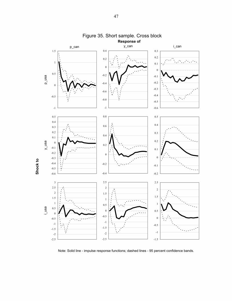
47

-1

-0.5

0

0.5

1

1.5

-1

-0.8

-0.6

-0.4

-0.2

0

0.2

0.4

-0.6

-0.5

-0.4

-0.3

-0.2

-0.1

0

0.1

0.2


p_us

a

Shoc

k to

Response of

-0.6

-0.5

-0.4

-0.3

-0.2

-0.1

0

0.1

0.2

0.3

0.4

0.5

-0.4

-0.2

0

0.2

0.4

0.6

0.8

-0.2

-0.1

0

0.1

0.2

0.3

0.4

0.5

y_us

a

-2.5

-2

-1.5

-1

-0.5

0

0.5

1

1.5

2

2.5

3

-2.5

-2

-1.5

-1

-0.5

0

0.5

1

1.5

2

2.5

-1.5

-1

-0.5

0

0.5

1

1.5

2

2.5

i_us

a


Figure 35. Short sample. Cross block

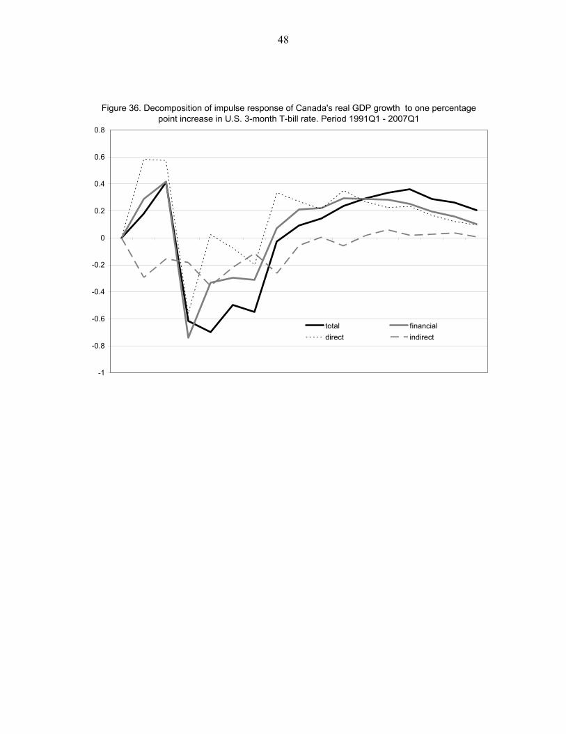
48

-1

-0.8

-0.6

-0.4

-0.2

0

0.2

0.4

0.6

0.8

total financialdirect indirect

Figure 36. Decomposition of impulse response of Canada's real GDP growth to one percentage point increase in U.S. 3-month T-bill rate. Period 1991Q1 - 2007Q1

49

Appendix Financial Conditions Indices Most financial conditions indices include a relatively small number (three to six) variables, such as official and/or market interest rates (always short-term, and sometimes also long-term), exchange rates, stock prices, and occasionally real estate prices, measures of money supply, and miscellaneous other variables. The index designers attempt to pick the “most representative” financial sector variables and argue that omitted asset prices and measures of credit are highly correlated with those included.21 According to Gauthier and others (2004), the Goldman Sachs FCI for the United States includes the real 3-month LIBOR, the real yield on long-term A-rated corporate bonds, the real trade-weighted exchange rate and the ratio of the equity market capitalization to nominal GDP. According to the same source, the Canadian FCI is a simple average of the real 3-month market rate, the yield curve, the real effective exchange rate, and a measure of stock valuation. While the construction of the U.S. index is described in some detail in Dudley and Hatzius (2000), there is no additional publicly available information on how the Canadian index is constructed. Given the paucity of information and the desire to produce compatible indices, we proceed in the following fashion. For the United States, we used the numbers graciously provided by Goldman Sachs. This series exhibits behavior similar, but not identical to that calculated on the basis of the formula in Dudley and Hatzius (2000), and the levels are different, as apparently the formula has been revised. Since the data provided do not cover the whole sample period, we have spliced it with the index based on the year 2000 formula. Finally, since the series thus constructed had a substantial downward trend, and it is hardly plausible that financial conditions in the United States have been loosening systematically over the past quarter century, the series was detrended. For Canada, we constructed the index from scratch on the basis of the available information. The real 3-month market rate was calculated by subtracting from the 3-month rate on prime commercial paper22 the year-on-year CPI inflation rate for the period that spans the current quarter. The CPI-based real effective exchange rate is taken from the IMF’s International Financial Statistics. The value of the S&P/TSX Composite Index is taken to be the measure of the stock market. The slope of the yield curve is calculated as the difference between the yields on the 10-year government bond and the 3-month T-bill. The inputs for the FCI are calculated as the deviation of the real interest rate from the period average; the percentage deviation of the real exchange rate from the period average; the deviation of the logarithm of the TSX index from the linear trend, multiplied by 100, with a reverse sign; and the yield curve slope, with the 21 An alternative approach, represented by English and others (2005), is to construct a “diffusion index” based on filtering the information contained in a large number of financial series.

22 This was the only series available for the whole sample period. That interest rate moves very closely with the three-month Canadian dollar LIBOR and the rates on three-month bankers’ acceptances for the periods where data is available.

50

opposite sign. The financial conditions index is the simple average of the above inputs. It is also demeaned, to provide an indication of how easy or tight financial conditions were in a given period relative to the average, but this has no impact on regression coefficients (other than the constants) or the impulse response functions. Figure A1 shows the behavior of the index and its components.

Figure A1. Canadian FCI and its components

-20

-15

-10

-5

0

5

10

15

Q1-

1981

Q4-

1981

Q3-

1982

Q2-

1983

Q1-

1984

Q4-

1984

Q3-

1985

Q2-

1986

Q1-

1987

Q4-

1987

Q3-

1988

Q2-

1989

Q1-

1990

Q4-

1990

Q3-

1991

Q2-

1992

Q1-

1993

Q4-

1993

Q3-

1994

Q2-

1995

Q1-

1996

Q4-

1996

Q3-

1997

Q2-

1998

Q1-

1999

Q4-

1999

Q3-

2000

Q2-

2001

Q1-

2002

Q4-

2002

Q3-

2003

Q2-

2004

Q1-

2005

Q4-

2005

Q3-

2006

r_market

reer

tsx

yield_curve

FCI

One can clearly take issue with the notion that an index thus constructed represents a true measure of financial conditions. For example, the Canadian dollar may appreciate because of high oil prices, and that equilibrium appreciation would not necessarily signal a tightening of financial conditions.23 It is also not clear whether an inverted yield curve means tighter financial conditions. Particularly for a given short-term rate, which is included in the index, more inversion means cheaper financing at the long end. The reason the slope of the yield curve is included in the index is probably because an inversion indicates market expectation of future loosening of monetary policy, and is sometimes viewed as a sign of an approaching recession. If that is the case, the inclusion of the yield curve in the FCI is perhaps a concession to improving its predictive ability for future growth while somewhat compromising its role as an indicator of current financial conditions. While these reservations would argue against including the yield curve slope in the FCI for the purposes of this paper, we wanted to stay as faithful to an independently constructed index as we possibly could. In addition, the variability of the yield 23 Similar concerns have led the Bank of Canada to discontinue its use of the monetary conditions index that featured the interest rate on commercial paper and the nominal effective exchange rate.

51

curve slope in Canada was smaller than that of any other component of the FCI, so its inclusion does not make much difference. More broadly, we do recognize various criticisms leveled against financial conditions indices, and for that reason include these indices in our robustness checks rather than the baseline specification. Figure A2 shows the US FCI (demeaned and detrended) and the Canadian FCI (with and without the slope of the yield curve in the formula). As one can see, U.S. and Canadian indices do not always move hand in hand. Indeed, the correlation between the two series over the sample period is only 9 percent—considerably smaller than the correlation between the 3-month T-bill rates (85 percent). Part of that probably reflects the different way the two indices have been constructed. Another reason is that changes in the bilateral exchange rate move the two indices in the opposite directions.

Figure A2. Canadian and U.S. FCI

-10

-8

-6

-4

-2

0

2

4

6

8

10

Q1-

1981

Q4-

1981

Q3-

1982

Q2-

1983

Q1-

1984

Q4-

1984

Q3-

1985

Q2-

1986

Q1-

1987

Q4-

1987

Q3-

1988

Q2-

1989

Q1-

1990

Q4-

1990

Q3-

1991

Q2-

1992

Q1-

1993

Q4-

1993

Q3-

1994

Q2-

1995

Q1-

1996

Q4-

1996

Q3-

1997

Q2-

1998

Q1-

1999

Q4-

1999

Q3-

2000

Q2-

2001

Q1-

2002

Q4-

2002

Q3-

2003

Q2-

2004

Q1-

2005

Q4-

2005

Q3-

2006

Can FCI

Can FCI (no yield curve)

US FCI demeaned

US FCI detrended

52

References Ambler, Steve, Emanuela Cardia, and Christian Zimmermann, 2004, “International Business Cycles: What are the Facts?”, Journal of Monetary Economics, Vol. 51, Issue 2, pp. 257–276. Calmès, Christian, 2004, “Regulatory Changes and Financial Structure: The Case of Canada,” Bank of Canada Working Paper 2004-26. Christiano, Lawrence J., Martin Eichenbaum, and Charles L. Evans, 1999, “Monetary Policy Shocks: What Have We Learned and to What End?” in John B. Taylor and Michael Woodford (eds.), Handbook of Macroeconomics, Vol. 1, Part 1. Cushman, David O., and Tao Zha, 1997, “Identifying Monetary Policy in a Small Open Economy under Flexible Exchange Rates,” Journal of Monetary Economics, Vol. 39, pp. 433–448. Dudley, William, and Jan Hatzius, 2000, “The Goldman Sachs Financial Conditions Index: The Right Tool for a New Monetary Policy Regime,” Goldman Sachs Global Economics Paper No. 44. Dungey, Mardi, and Adrian Pagan, 2000, “A Structural VAR Model of the Australian Economy,” Economic Record, Vol. 81, pp. 321–342. English, William, Kostas Tsatsaronis, and Edda Zoli, 2005, “Assessing the Predictive Power of Measures of Financial Conditions for Macroeconomic Variables,” BIS Papers No. 22. Freedman, Charles, and Walter Engert, 2003, “Financial Developments in Canada: Past Trends and Future Challenges,” Bank of Canada Review, Summer 2003, pp. 3–16. Gauthier, Céline, Christopher Graham, and Ying Liu, 2004, “Financial Conditions Indexes for Canada,” Bank of Canada Working Paper 2004-22. Hamilton, James D., 1994, Time Series Analysis, Princeton University Press. Issa, Ramzi, Robert Lafrance, and John Murray, 2006, “The Turning Black Tide: Energy Prices and the Canadian Dollar,” Bank of Canada Working Paper 2006-29. Sellin, Peter, 2001, “Monetary Policy and the Stock Market: Theory and Empirical Evidence,” Journal of Economic Surveys, Vol. 15, Issue 4, pp. 491–541. Sims, Christopher A., 1992, “Interpreting the Macroeconomic Time Series Facts: The Effects of Monetary Policy,” European Economic Review, Vol. 36, pp. 975–1011. Stock, James H., and Mark W. Watson, 2002, “Has the Business Cycle Changed and Why?”, 2002 NBER Macroeconomics Annual, Number 17, pp. 159–218.

Documents

Real Implications of Financial Linkages Between · PDF fileReal Implications of Financial Linkages between ... cost of funds for Canadian companies raising capital in ... main source