Real Exchange Rates and Primary Commodity Prices Exchange Rates and Primary Commodity ... Real Exchange Rates and Primary Commodity Prices ... against the US dollar can be accounted

Real Exchange Rates and Primary Commodity Prices

Joao Ayres Inter-American Development Bank

Constantino Hevia

Universidad Torcuato Di Tella

Juan Pablo Nicolini Federal Reserve Bank of Minneapolis and Universidad Torcuato Di Tella

Working Paper 743

November 2017

DOI: https://doi.org/10.21034/wp.743 Keywords: Primary commodity prices; Real exchange rate disconnect puzzle JEL classification: F31, F41 The views expressed herein are those of the authors and not necessarily those of the Federal Reserve Bank of Minneapolis or the Federal Reserve System. __________________________________________________________________________________________

Federal Reserve Bank of Minneapolis • 90 Hennepin Avenue • Minneapolis, MN 55480-0291

https://www.minneapolisfed.org/research/

https://doi.org/10.21034/wp.743

https://www.minneapolisfed.org/research/

Real Exchange Rates and PrimaryCommodity Prices ∗

Joao Ayres

Inter-American Development Bank

Constantino Hevia

Universidad Torcuato Di Tella

Juan Pablo Nicolini

Federal Reserve Bank of Minneapolis and Universidad Torcuato Di Tella

November 14, 2017

Abstract

In this paper, we show that a substantial fraction of the volatility of real exchange

rates between developed economies such as Germany, Japan, and the United Kingdom

against the US dollar can be accounted for by shocks that affect the prices of primary

commodities such as oil, aluminum, maize, or copper. Our analysis implies that exist-

ing models used to analyze real exchange rates between large economies that mostly

focus on trade between differentiated final goods could benefit, in terms of matching

the behavior of real exchange rates, by also considering trade in primary commodities.

Keywords: primary commodity prices, real exchange rate disconnect puzzle.

JEL classification: F31, F41.

∗We thank Manuel Amador, Roberto Chang, Juan Carlos Conesa, Deepa Datta, Jonathan Heathcote,Patrick Kehoe, Tim Kehoe, Albert Marcet, Enrique Mendoza, Martin Sola, Esteban Rossi-Hansberg, andMartin Uribe for comments. The views expressed herein are those of the authors and not necessarily those ofthe Federal Reserve Bank of Minneapolis, the Federal Reserve System, or the Inter-American DevelopmentBank.

1

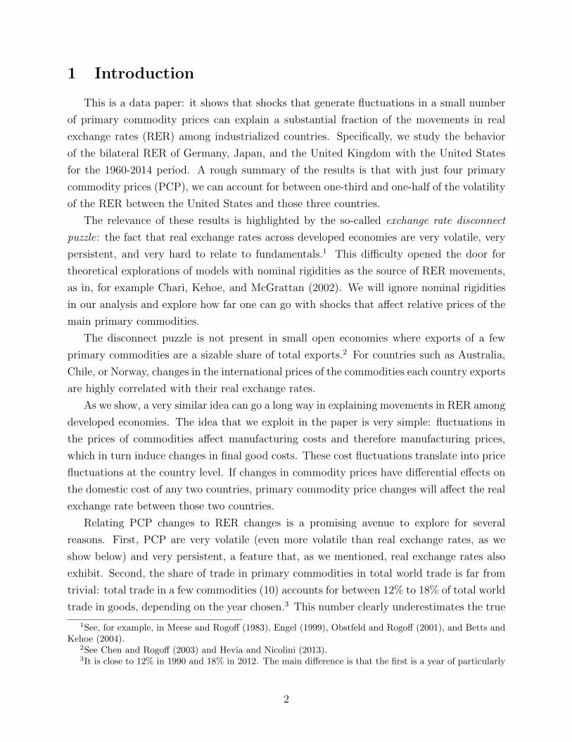
1 Introduction

This is a data paper: it shows that shocks that generate fluctuations in a small number

of primary commodity prices can explain a substantial fraction of the movements in real

exchange rates (RER) among industrialized countries. Specifically, we study the behavior

of the bilateral RER of Germany, Japan, and the United Kingdom with the United States

for the 1960-2014 period. A rough summary of the results is that with just four primary

commodity prices (PCP), we can account for between one-third and one-half of the volatility

of the RER between the United States and those three countries.

The relevance of these results is highlighted by the so-called exchange rate disconnect

puzzle: the fact that real exchange rates across developed economies are very volatile, very

persistent, and very hard to relate to fundamentals.1 This difficulty opened the door for

theoretical explorations of models with nominal rigidities as the source of RER movements,

as in, for example Chari, Kehoe, and McGrattan (2002). We will ignore nominal rigidities

in our analysis and explore how far one can go with shocks that affect relative prices of the

main primary commodities.

The disconnect puzzle is not present in small open economies where exports of a few

primary commodities are a sizable share of total exports.2 For countries such as Australia,

Chile, or Norway, changes in the international prices of the commodities each country exports

are highly correlated with their real exchange rates.

As we show, a very similar idea can go a long way in explaining movements in RER among

developed economies. The idea that we exploit in the paper is very simple: fluctuations in

the prices of commodities affect manufacturing costs and therefore manufacturing prices,

which in turn induce changes in final good costs. These cost fluctuations translate into price

fluctuations at the country level. If changes in commodity prices have differential effects on

the domestic cost of any two countries, primary commodity price changes will affect the real

exchange rate between those two countries.

Relating PCP changes to RER changes is a promising avenue to explore for several

reasons. First, PCP are very volatile (even more volatile than real exchange rates, as we

show below) and very persistent, a feature that, as we mentioned, real exchange rates also

exhibit. Second, the share of trade in primary commodities in total world trade is far from

trivial: total trade in a few commodities (10) accounts for between 12% to 18% of total world

trade in goods, depending on the year chosen.3 This number clearly underestimates the true

1See, for example, in Meese and Rogoff (1983), Engel (1999), Obstfeld and Rogoff (2001), and Betts andKehoe (2004).

2See Chen and Rogoff (2003) and Hevia and Nicolini (2013).3It is close to 12% in 1990 and 18% in 2012. The main difference is that the first is a year of particularly

2

share of commodities, since trade shares are not value-added measures. Thus, when steel is

exported, it is fully counted as a manufactured good, even though an important component

of its cost depends on iron. The same happens when a car is exported. Third, primary

commodities are at the bottom of the production chain, so they directly affect final good

prices.4 In addition, they may directly affect the prices of other domestic inputs – such as

some types of labor and services in general – that are used jointly with primary commodities

in the production of intermediate goods, and thus they may indirectly affect the costs of

final goods. Because just a few commodities make up a high share of total trade, we only

need to focus on a handful of prices. Finally, it is well known that the law of one price on

those primary commodities holds, so no ambiguity with respect to their tradability exists.

The literature on RER has struggled to separate the set of final goods into two categories:

the ones that are traded, for which the law of one price is assumed to hold, and the ones

that are not. We only need to assume that for the few commodities we analyze, the law of

one price holds, and it is precisely for these prices that independent evidence that the law

of one price holds is the strongest.

The exchange rate disconnect puzzle has been widely studied in the literature. Two

recent attempts at quantitatively explaining several facts related to the puzzle are Itskhoki

and Mukhin (2017), and Eaton, Kortum, and Neiman (2016). They provide very good

descriptions of the state of the literature. The connection between RER and PCP has largely

been ignored for the countries we focus on, and not only on the empirical side. Ever since

the seminal contribution of Obstfeld and Rogoff (1995), the theoretical literature developed

to study RER between the countries we consider in this paper has focused exclusively on

the production and trade of final goods. Our evidence suggests that theoretical models of

RER among developed economies that ignore primary commodity markets may fall short of

providing a comprehensive explanation of RER movements.

In Section 2 we describe the data and motivate the analysis by showing some descriptive

statistics. We also discuss several issues related to the empirical methodology used in the

paper. In Section 3 we present the main results. In Section 4 we perform a series of Monte

Carlo exercises to address issues related to small sample properties of the moments we

estimate in Section 3. In Section 5 we partially spell out the production side of a totally

standard model of an open economy that makes explicit the production of commodities and

the use of commodities in the production of manufactured goods. We derive an equilibrium

condition relating the bilateral RER between two countries to PCP that, in the case of

low primary commodity prices, while the second is a period of particularly high prices.4This direct effect is substantial enough for monetary authorities in developed countries to focus attention

on measures of “core” inflation, which abstract from the “volatile” effect of primary commodity prices (foodand energy).

3

Cobb-Douglas production functions, is linear in the logarithms of the variables. This log-

linear relationship rationalizes the one used in the empirical analysis presented in Section 3.

Finally, in Section 6, we present an additional exercise, motivated by the model of Section 5.

A brief discussion of the implications of the results is presented in a final concluding section.

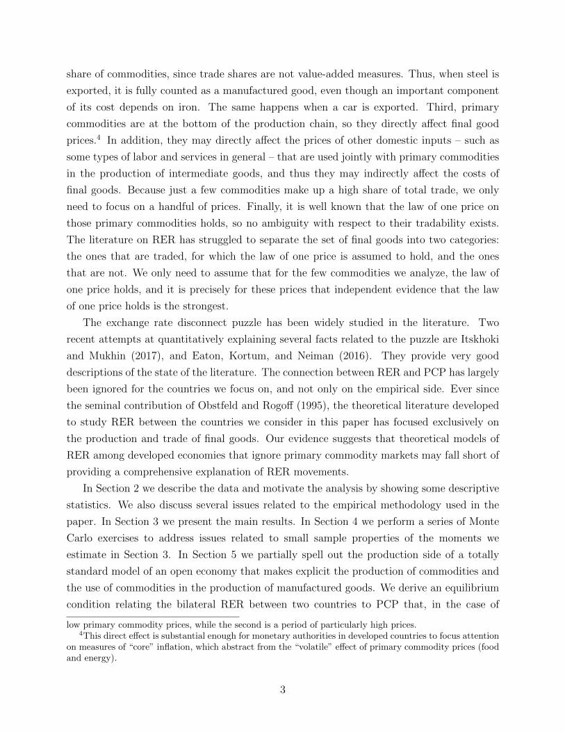
2 The data and the methodology

We collected monthly data on consumer price levels and nominal exchange rates for

the United States, Germany, the United Kingdom, and Japan. The bilateral RER are

defined as the nominal exchange rates between Germany (DEU), Japan (JPN), and the

United Kingdom (UK) against the US dollar multiplied by the ratio of CPIs. In the case of

Germany, we use the mark until 2000 and the euro thereafter. In addition, we collected price

data for the 10 primary commodities with the largest shares in world trade in 1990 and for

which monthly price data are available from January 1960 to December 2014. Appendix A

includes a detailed description of the data. Table 1 shows the selected primary commodities

and their respective definitions and shares in world trade.5

Table 1: Primary Commodities List

(%) share of (%) share ofworld trade SITC world trade SITC

Commodity in 1990 (rev.3) Commodity in 1990 (rev.3)

(1) Petroleum 7.22 33 (6) Gold 0.42 971.01(2) Fish 1.05 03 (7) Wheat 0.35 041(3) Meat 0.89 011/012 (8) Maize 0.28 044(4) Aluminium 0.49 285.1/684.1 (9) Timber 0.26 24(5) Copper 0.45 283.1/682.1 (10) Cotton 0.22 263

Note: SITC (rev3) stands for Standard International Trade Classification (revision 3).Source: Comtrade.

As already mentioned, the bilateral real exchange rates between the countries we analyze

are known to be very persistent and volatile. This is one of the properties that make PCP

attractive to relate to RER, since they are also known to be persistent and volatile: if shocks

to PCP are to account for a large share of the volatility of real exchange rates, it must also

share these same features. We now show that this is indeed the case.

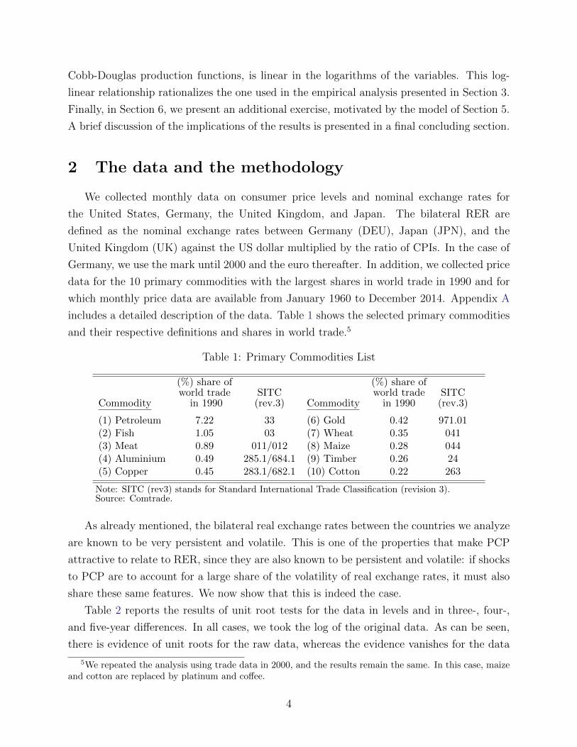
Table 2 reports the results of unit root tests for the data in levels and in three-, four-,

and five-year differences. In all cases, we took the log of the original data. As can be seen,

there is evidence of unit roots for the raw data, whereas the evidence vanishes for the data

5We repeated the analysis using trade data in 2000, and the results remain the same. In this case, maizeand cotton are replaced by platinum and coffee.

4

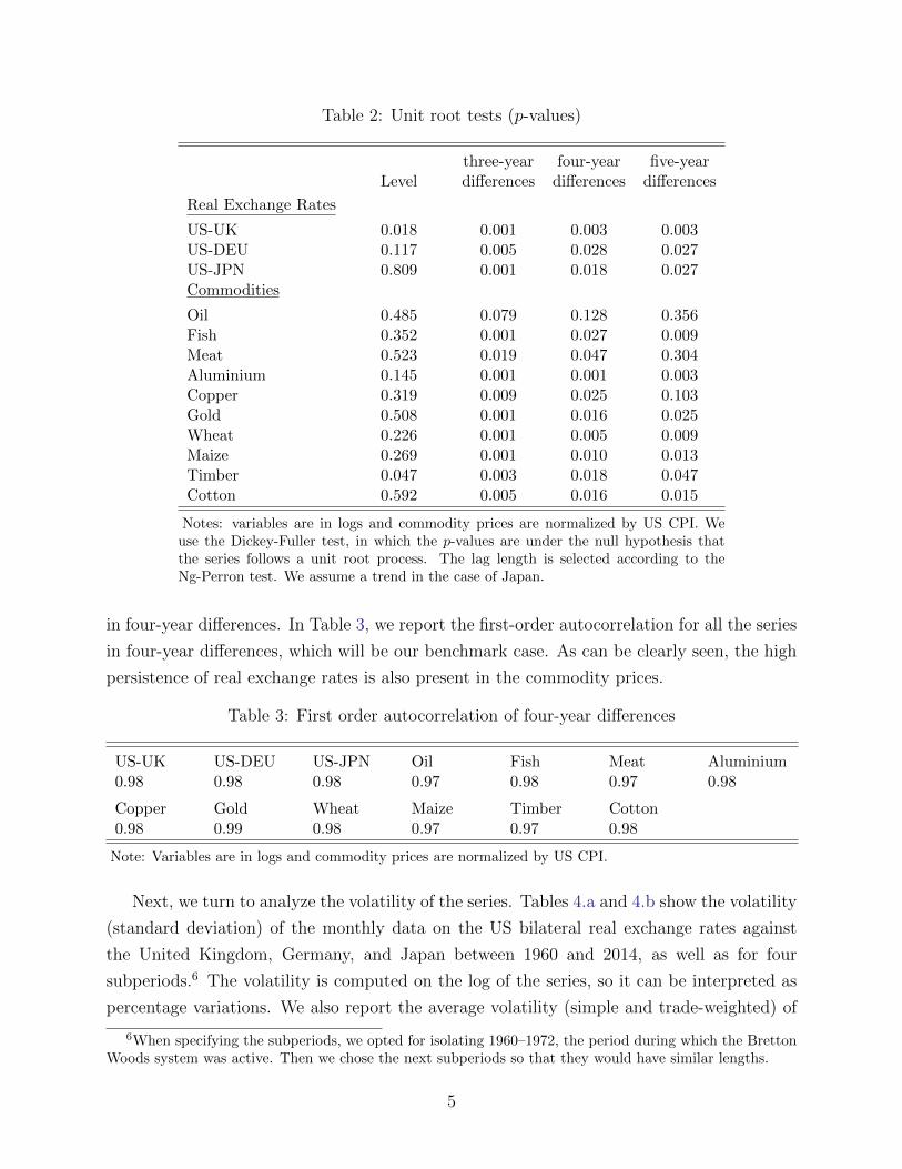
Table 2: Unit root tests (p-values)

three-year four-year five-yearLevel differences differences differences

Real Exchange Rates

US-UK 0.018 0.001 0.003 0.003US-DEU 0.117 0.005 0.028 0.027US-JPN 0.809 0.001 0.018 0.027Commodities

Oil 0.485 0.079 0.128 0.356Fish 0.352 0.001 0.027 0.009Meat 0.523 0.019 0.047 0.304Aluminium 0.145 0.001 0.001 0.003Copper 0.319 0.009 0.025 0.103Gold 0.508 0.001 0.016 0.025Wheat 0.226 0.001 0.005 0.009Maize 0.269 0.001 0.010 0.013Timber 0.047 0.003 0.018 0.047Cotton 0.592 0.005 0.016 0.015

Notes: variables are in logs and commodity prices are normalized by US CPI. Weuse the Dickey-Fuller test, in which the p-values are under the null hypothesis thatthe series follows a unit root process. The lag length is selected according to theNg-Perron test. We assume a trend in the case of Japan.

in four-year differences. In Table 3, we report the first-order autocorrelation for all the series

in four-year differences, which will be our benchmark case. As can be clearly seen, the high

persistence of real exchange rates is also present in the commodity prices.

Table 3: First order autocorrelation of four-year differences

US-UK US-DEU US-JPN Oil Fish Meat Aluminium0.98 0.98 0.98 0.97 0.98 0.97 0.98

Copper Gold Wheat Maize Timber Cotton0.98 0.99 0.98 0.97 0.97 0.98

Note: Variables are in logs and commodity prices are normalized by US CPI.

Next, we turn to analyze the volatility of the series. Tables 4.a and 4.b show the volatility

(standard deviation) of the monthly data on the US bilateral real exchange rates against

the United Kingdom, Germany, and Japan between 1960 and 2014, as well as for four

subperiods.6 The volatility is computed on the log of the series, so it can be interpreted as

percentage variations. We also report the average volatility (simple and trade-weighted) of

6When specifying the subperiods, we opted for isolating 1960–1972, the period during which the BrettonWoods system was active. Then we chose the next subperiods so that they would have similar lengths.

5

the prices of the commodities listed in Table 1. Table 4.a presents the volatilities for the raw

data, and Table 4.b presents the volatilities for the data in four-year differences.

As can be seen, the volatility of PCP is substantially higher than that of RER.7 In

addition, it is apparent that in the subperiods in which the volatility of PCP is high, so is

the volatility of the RER. We find this issue particularly interesting, since the substantial

increase in the volatility of real exchange rates after the breakdown of the Bretton-Woods

system of fixed exchange rates is accompanied by an equally substantial increase in the

volatility of commodity prices. The conventional interpretation has been that the increase

in volatility after 1972 was the result of the regime change from fixed to flexible exchange

rates.8 An alternative interpretation is that the fundamentals that cause real exchange rates

and commodity prices to move together were much more volatile after 1973 than before.

To the extent that PCP are independent of the exchange rate regimes, our evidence points

toward an alternative explanation of the increase in volatility post Bretton-Woods.

Note also that the reduction in real exchange rate volatility that ensued after the mid-

1980s is also accompanied by a reduction in the volatility of commodity prices. As a com-

plementary piece of evidence, Figure 1 shows rolling volatilities computed using windows of

10 years of data for the three real exchange rates and for the average volatility of the 10

primary commodity prices. The figure clearly points toward a positive association between

the volatilities of the real exchange rate and commodity prices.9 This positive association

reinforces, in our view, the interest in associating RER with PCP.

Finally, in Table 5 we show the simple correlations of each of the bilateral RER and all

the commodity prices we use. As can be seen, all simple correlations between the prices and

the RER are sizable. In addition, the correlations across the PCP are also sizable in many

cases.

2.1 Methodology

Our goal is to assess how much of the variability of the US bilateral real exchange rates

with the United Kingdom, Germany, and Japan can be accounted for by a set of primary

commodity prices. In following the small open economy literature, and pairing the United

States and United Kingdom as an example, we analyze the following regression equation:

lnPUSAt − lnPUK

t + lnSt = βpX,USAt + vt. (1)

7This is also the case for small open economies, where the ratio of the volatility of the relevant PCP isbetween 2.5 and 3.5 the volatility of the RER. These values are similar to the ones that can be obtainedfrom Table 4.

8See Mussa (1986).9The correlations are 0.40, 0.54, and 0.39 for the United Kingdom, Germany, and Japan, respectively.

6

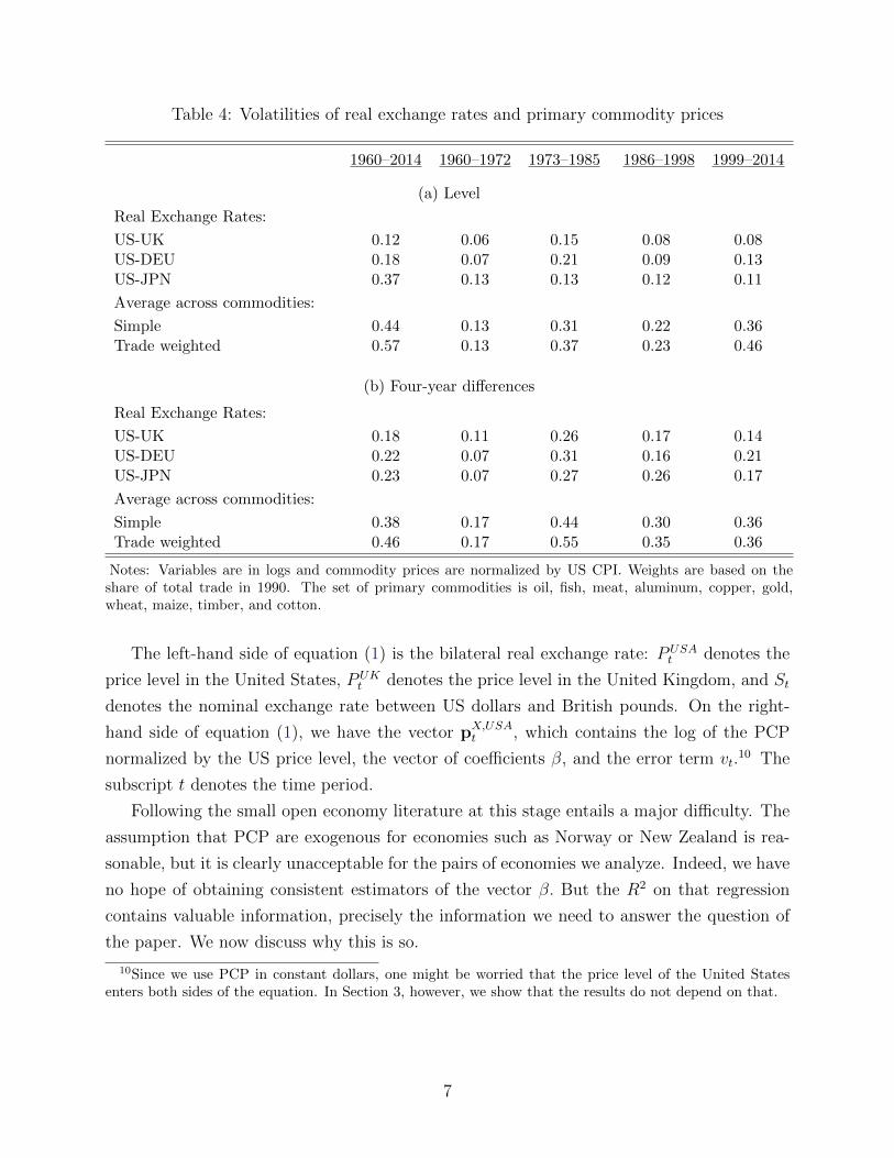
Table 4: Volatilities of real exchange rates and primary commodity prices

1960–2014 1960–1972 1973–1985 1986–1998 1999–2014

(a) Level

Real Exchange Rates:

US-UK 0.12 0.06 0.15 0.08 0.08US-DEU 0.18 0.07 0.21 0.09 0.13US-JPN 0.37 0.13 0.13 0.12 0.11

Average across commodities:

Simple 0.44 0.13 0.31 0.22 0.36Trade weighted 0.57 0.13 0.37 0.23 0.46

(b) Four-year differences

Real Exchange Rates:

US-UK 0.18 0.11 0.26 0.17 0.14US-DEU 0.22 0.07 0.31 0.16 0.21US-JPN 0.23 0.07 0.27 0.26 0.17

Average across commodities:

Simple 0.38 0.17 0.44 0.30 0.36Trade weighted 0.46 0.17 0.55 0.35 0.36

Notes: Variables are in logs and commodity prices are normalized by US CPI. Weights are based on theshare of total trade in 1990. The set of primary commodities is oil, fish, meat, aluminum, copper, gold,wheat, maize, timber, and cotton.

The left-hand side of equation (1) is the bilateral real exchange rate: PUSAt denotes the

price level in the United States, PUKt denotes the price level in the United Kingdom, and St

denotes the nominal exchange rate between US dollars and British pounds. On the right-

hand side of equation (1), we have the vector pX,USAt , which contains the log of the PCP

normalized by the US price level, the vector of coefficients β, and the error term vt.10 The

subscript t denotes the time period.

Following the small open economy literature at this stage entails a major difficulty. The

assumption that PCP are exogenous for economies such as Norway or New Zealand is rea-

sonable, but it is clearly unacceptable for the pairs of economies we analyze. Indeed, we have

no hope of obtaining consistent estimators of the vector β. But the R2 on that regression

contains valuable information, precisely the information we need to answer the question of

the paper. We now discuss why this is so.

10Since we use PCP in constant dollars, one might be worried that the price level of the United Statesenters both sides of the equation. In Section 3, however, we show that the results do not depend on that.

7

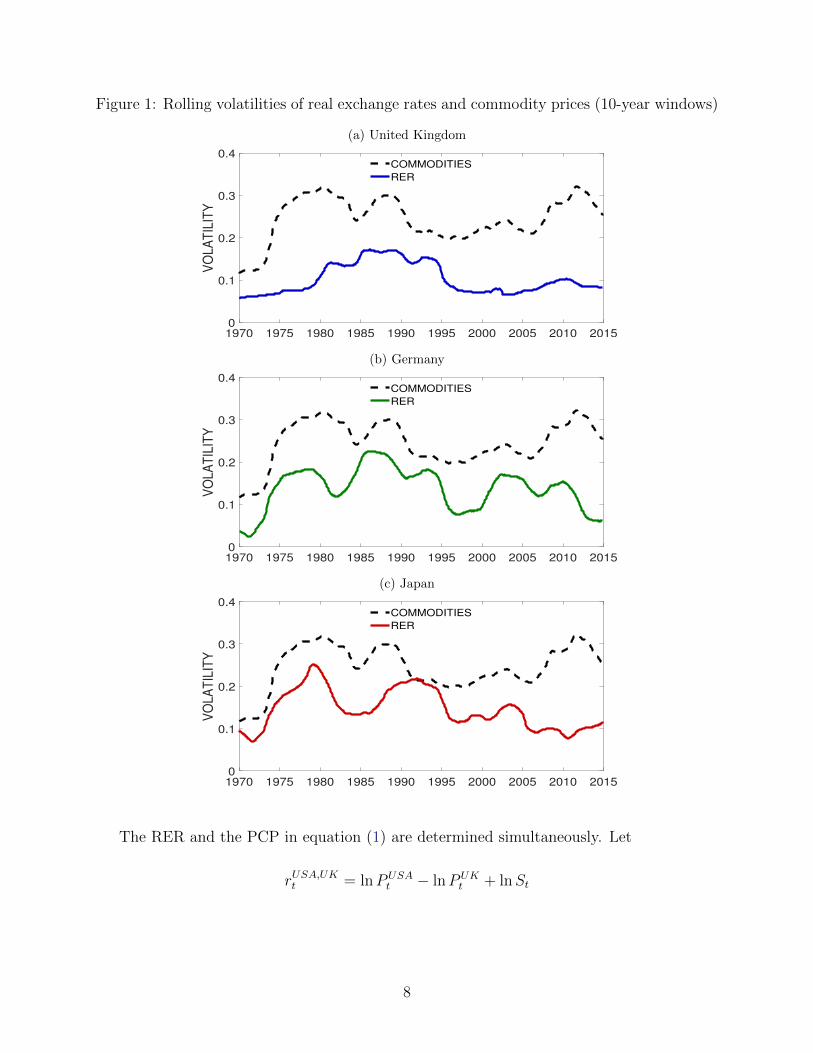
Figure 1: Rolling volatilities of real exchange rates and commodity prices (10-year windows)

(a) United Kingdom

1970 1975 1980 1985 1990 1995 2000 2005 2010 20150

0.1

0.2

0.3

0.4

VO

LA

TIL

ITY

COMMODITIES

RER

(b) Germany

1970 1975 1980 1985 1990 1995 2000 2005 2010 20150

0.1

0.2

0.3

0.4

VO

LA

TIL

ITY

COMMODITIES

RER

(c) Japan

1970 1975 1980 1985 1990 1995 2000 2005 2010 20150

0.1

0.2

0.3

0.4

VO

LA

TIL

ITY

COMMODITIES

RER

The RER and the PCP in equation (1) are determined simultaneously. Let

rUSA,UKt = lnPUSAt − lnPUK

t + lnSt

8

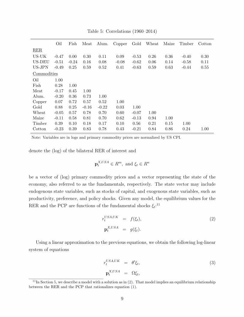
Table 5: Correlations (1960–2014)

Oil Fish Meat Alum. Copper Gold Wheat Maize Timber Cotton

RER

US-UK -0.47 0.00 0.30 0.11 0.09 -0.53 0.26 0.36 -0.40 0.30US-DEU -0.51 -0.24 0.16 0.08 -0.08 -0.62 0.06 0.14 -0.58 0.11US-JPN -0.49 0.25 0.59 0.52 0.41 -0.63 0.59 0.63 -0.44 0.55

Commodities

Oil 1.00Fish 0.28 1.00Meat -0.17 0.45 1.00Alum. -0.20 0.36 0.73 1.00Copper 0.07 0.72 0.57 0.52 1.00Gold 0.88 0.25 -0.16 -0.22 0.03 1.00Wheat -0.05 0.57 0.78 0.70 0.60 -0.07 1.00Maize -0.11 0.58 0.81 0.70 0.62 -0.13 0.94 1.00Timber 0.39 0.10 0.18 0.17 0.10 0.56 0.21 0.15 1.00Cotton -0.23 0.39 0.83 0.78 0.43 -0.21 0.84 0.86 0.24 1.00

Note: Variables are in logs and primary commodity prices are normalized by US CPI.

denote the (log) of the bilateral RER of interest and

pX,USAt ∈ Rm, and ξt ∈ Rn

be a vector of (log) primary commodity prices and a vector representing the state of the

economy, also referred to as the fundamentals, respectively. The state vector may include

endogenous state variables, such as stocks of capital, and exogenous state variables, such as

productivity, preference, and policy shocks. Given any model, the equilibrium values for the

RER and the PCP are functions of the fundamental shocks ξt:11

rUSA,UKt = f(ξt), (2)

pX,USAt = g(ξt).

Using a linear approximation to the previous equations, we obtain the following log-linear

system of equations

rUSA,UKt = θ′ξt, (3)

pX,USAt = Ωξt,

11In Section 5, we describe a model with a solution as in (2). That model implies an equilibrium relationshipbetween the RER and the PCP that rationalizes equation (1).

9

where θ is an n× 1 vector, Ω is an m× n matrix, and variables are measured as deviations

from their long-run means. We treat the fundamental shocks of the economy as unobserved,

so we can interpret the state variables ξt as orthogonal with an identity covariance matrix

without loss of generality.12

Consider projecting the real exchange rate rUSA,UKt onto the commodity prices pX,USAt ,

Proj(rUSA,UKt |pX,USAt ) = β′pX,USAt .

By the orthogonality principle, β solves E[rUSA,UKt (pX,USAt )′] = β′E[pX,USAt (pX,USAt )′]. Using

that in equilibrium the RER and the PCP are related to the fundamental shocks through

equation (3), E[rUSA,UKt (pX,USAt )′] = θ′Ω′ and E[pX,USAt (pX,USAt )′] = ΩΩ′, which gives β′ =

(θ′Ω′)(ΩΩ′)−1. Finally, using pX,USAt = Ωξt, the projection of the real exchange rate onto the

commodity prices is equivalent to decomposing the real exchange rate into two orthogonal

components:

rUSA,UKt = β′Ωξt + (θ′ − β′Ω)ξt. (4)

The first term on the right side of equation (4) is the component of the real exchange rate

that is correlated with primary commodity prices. It measures how much of the variability

of the real exchange rate can be accounted for by fundamental shocks that affect primary

commodity prices. The second component of the projection is orthogonal to the first and

measures how much of the variability of the real exchange rate is accounted for by fundamen-

tal shocks that do not manifest themselves as fluctuations in commodity prices correlated

with the real exchange rate. In terms of this decomposition, the R2 of the regression (1) can

be written as

R2 =E[β′Ωξtξt

′Ω′β]

E[(θ′ξtξt′θ)]

=β′ΩΩ′β

θ′θ. (5)

The underlying (implicit) assumption in much of the literature on bilateral real exchange

rates between developed countries is that the component associated with commodity prices,

β′Ωξt, can be safely ignored. We can express this no-relevance-of-commodities assumption

as the requirement that the R2 of the regression of real exchange rates on commodity prices

is zero, which is true whenever β′Ω = 0.

Let state variables be divided into two sets as ξt = [ξ′1t ξ′2t]′, so that rUSA,UKt = θ′1ξ1t+θ

′2ξ2t

and pX,USAt = Ω1ξ1t+Ω2ξ2t. It then follows that β′Ω = θ′1Ω1+θ′2Ω2. A necessary and sufficient

condition for the R2 of the regression to be zero is thus

θ1Ω1 = −θ2Ω2.

12If the shocks ξt have a nondiagonal covariance matrix E(ξtξ′t) = Σ, we can create an observationally

equivalent system with orthogonal state variables by letting ξt = Σ−1/2ξt, θ′ = θ′Σ1/2, and Ω = ΩΣ1/2.

10

A sufficient condition for this equality to hold is that θ1 = 0 and Ω2 = 0. This implies

an equilibrium with a block-recursive structure in which the set of state variables that de-

termine the real exchange rate are different from (and orthogonal to) those that determine

primary commodity prices. If these conditions do not hold, then commodity prices will be

(generically) correlated with the real exchange rate.

Measuring how much of the variability of the RER can be explained by this common

component – the R2 of equation (1) – is the objective of the following sections.

2.1.1 Higher-order terms

Linear approximations work well following shocks that imply small deviations from the

steady state. The large and persistent movements in both RER and PCP imply that the

approximation error may be large, so that second-order effects may be important to under-

stand the comovement between the RER and the PCP. One way out of this would be to

incorporate nonlinear terms in the regression equation (1). We view this paper as a first step

toward understanding the role that PCP may play in helping us to understand the large and

persistent movements in RER. We opted for simplicity, so we will only consider the linear

terms in the analysis that follows. Accordingly, the interpretation of the R2s we present

below can be seen as a lower bound on the fraction of the volatility of the RER that can be

accounted for by shocks that also move the PCP.

2.1.2 Time-varying coefficients

The coefficients in the linearized version (3) are evaluated at the equilibrium around which

the linearization is made. The economies we are about to study have experienced major

transformations during the more than five decades that cover the period we study. These

transformations have changed not only the production structures but also the trade patterns.

As such, it is reasonable to imagine that the equilibrium around which the linearization is

made in the 1960s is different from the one in the 1980s.13 Thus, there is no reason to believe

that those coefficients would remain constant over time. In order to capture this possibility,

we present our results for the whole period, but also for several subperiods. We also use this

idea to motivate the out-of-sample fit exercises we do in the next section.

13The model in Section 5 makes these statements precise.

11

3 Results

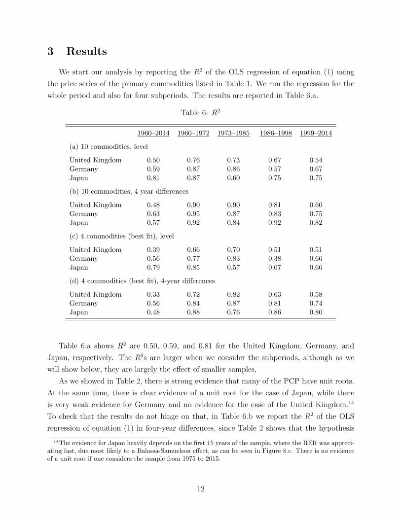
We start our analysis by reporting the R2 of the OLS regression of equation (1) using

the price series of the primary commodities listed in Table 1. We run the regression for the

whole period and also for four subperiods. The results are reported in Table 6.a.

Table 6: R2

1960–2014 1960–1972 1973–1985 1986–1998 1999–2014

(a) 10 commodities, level

United Kingdom 0.50 0.76 0.73 0.67 0.54Germany 0.59 0.87 0.86 0.57 0.67Japan 0.81 0.87 0.60 0.75 0.75

(b) 10 commodities, 4-year differences


(c) 4 commodities (best fit), level


(d) 4 commodities (best fit), 4-year differences


Table 6.a shows R2 are 0.50, 0.59, and 0.81 for the United Kingdom, Germany, and

Japan, respectively. The R2s are larger when we consider the subperiods, although as we

will show below, they are largely the effect of smaller samples.

As we showed in Table 2, there is strong evidence that many of the PCP have unit roots.

At the same time, there is clear evidence of a unit root for the case of Japan, while there

is very weak evidence for Germany and no evidence for the case of the United Kingdom.14

To check that the results do not hinge on that, in Table 6.b we report the R2 of the OLS

regression of equation (1) in four-year differences, since Table 2 shows that the hypothesis

14The evidence for Japan heavily depends on the first 15 years of the sample, where the RER was appreci-ating fast, due most likely to a Balassa-Samuelson effect, as can be seen in Figure 8.c. There is no evidenceof a unit root if one considers the sample from 1975 to 2015.

12

of unit root processes can be easily rejected for all three RER in this case.15 One could

use higher-frequency data by taking differences over a shorter horizon. However, we are

interested in the relatively long swings exhibited by the RER, those that last over a few

years, and that is why we focus on the four-year differences. For the interested reader, we

show in Appendix C the relationship between the R2 depicted in Table 6.d in the period

1960–2014 and the number of months for which we take the differences.

The results in Table 6.b show that PCP still account for between 48% and 57% of the

real exchange rate variation when we use the data in four-year differences. The R2 of the

regression for the whole period is smaller in the case of Japan (0.57 versus 0.81), which is

the country for which the evidence of a unit root in the RER is very strong. For the other

two countries, the differences are minimal.

As we showed in Table 5, the prices of the commodities we are using are well known to be

highly correlated. One could then guess that it is possible to account for a large fraction of

the real exchange rate volatility even if we considerably reduce the number of PCP. To show

this, we start by running the regression with 10 PCP, and then we pick the 4 with highest

t-statistics.16 The results with the data in levels are reported in Table 6.c, and the results

with the data in four-year differences are reported in Table 6.d. Tables 12–14 in Appendix

D report the coefficients of the regressions in Tables 6.c and 6.d.17

Tables 6.c and 6.d show that by selecting only four commodity price series, we can still

account for between 39% and 79% of the volatility of real exchange rates in levels, and for

between 33% and 56% of the volatility of real exchange rates in four-year differences. As

before, the problem of the unit root seems to be relevant only for the case of Japan. It

is also important to emphasize that PCP can account for a large share of real exchange

rate fluctuations in all subperiods we consider, and, in particular, there are no systematic

differences in the relationship between PCP and real exchange rates before and after the

Bretton Woods system. This goes in line with the alternative hypothesis about the increase

in real exchange rate volatility following 1972: that it coincided with an increase in the

volatility of fundamentals.

Finally, Figure 2 plots the data versus the respective fitted values for the regressions in

four-year differences for the cases of both 10 and 4 PCPs, and also reports the respective

correlation between the data and fitted values (equivalent to the square root of the R2).18

15Cointegration tests such as Johansen (1991) or Stock and Watson (1993) do not provide evidence ofcointegration between real exchange rates and primary commodity prices.

16Throughout the paper, we compute t-statistics using the Newey-West heteroskedasticity-and-autocorrelation-consistent standard errors.

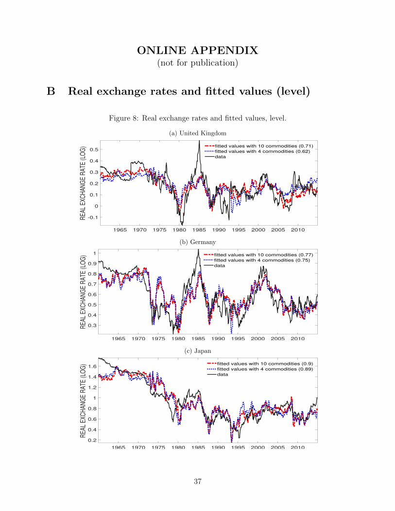
17In Appendix E we also show the results for the case in which we choose three commodities.18For the case of the data in levels, see Figure 8 in Appendix B. The results are very similar, except for

Japan, which is the country for which the unit root evidence is very high.

13

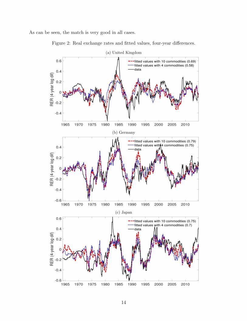
As can be seen, the match is very good in all cases.

Figure 2: Real exchange rates and fitted values, four-year differences.

(a) United Kingdom

1965 1970 1975 1980 1985 1990 1995 2000 2005 2010

-0.4

-0.2

0

0.2

0.4

0.6

RE

R (

4-y

ea

r lo

g d

if)

fitted values with 10 commodities (0.69)


data

(b) Germany

1965 1970 1975 1980 1985 1990 1995 2000 2005 2010-0.6

-0.4

-0.2

0

0.2

0.4

RE

R (

4-y

ea

r lo

g d

if)



data

(c) Japan

1965 1970 1975 1980 1985 1990 1995 2000 2005 2010-0.6

-0.4

-0.2

0

0.2

0.4

0.6

RE

R (

4-y

ea

r lo

g d

if)



data

14

One concern about regression (1) is that the variables are expressed in constant US

dollars, so the US CPI appears on both sides of the equation. If its volatility is sufficiently

large relative to the volatility of the nominal exchange rate and foreign CPI, that would

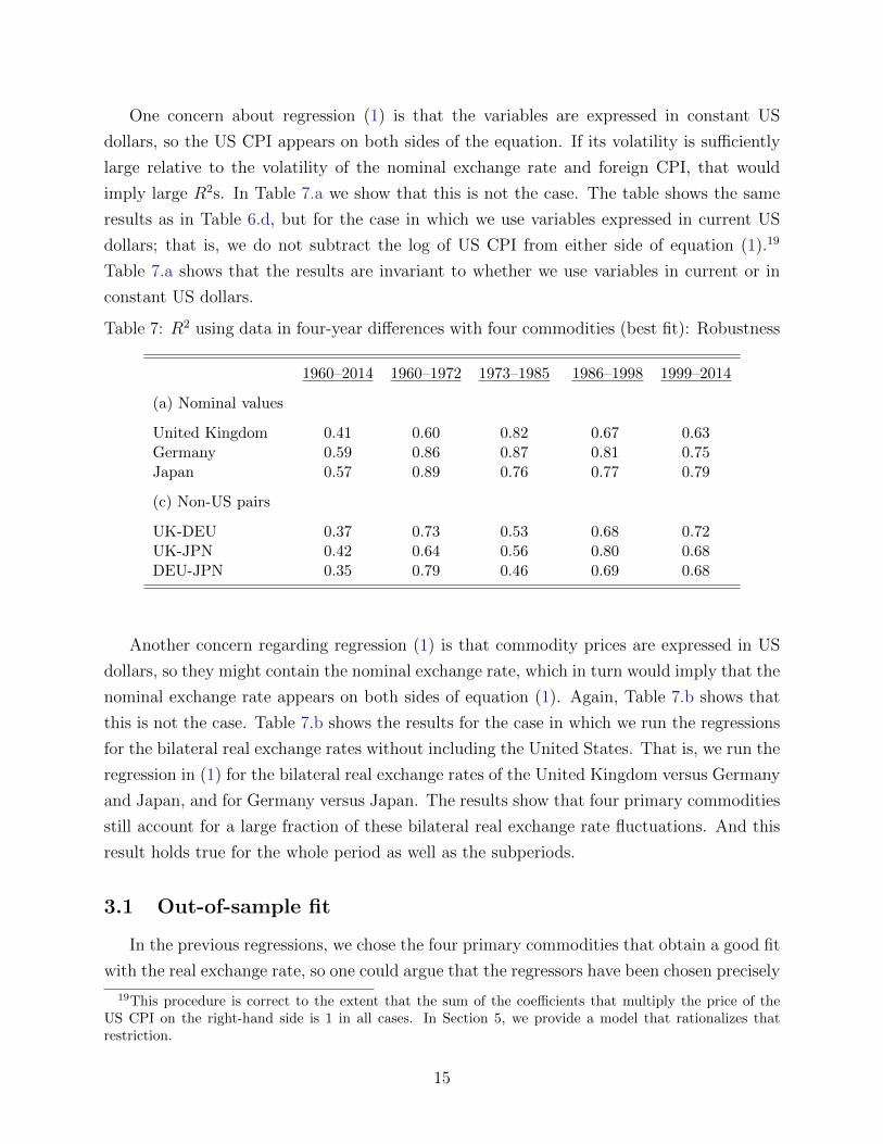
imply large R2s. In Table 7.a we show that this is not the case. The table shows the same

results as in Table 6.d, but for the case in which we use variables expressed in current US

dollars; that is, we do not subtract the log of US CPI from either side of equation (1).19

Table 7.a shows that the results are invariant to whether we use variables in current or in

constant US dollars.

Table 7: R2 using data in four-year differences with four commodities (best fit): Robustness

1960–2014 1960–1972 1973–1985 1986–1998 1999–2014

(a) Nominal values


(c) Non-US pairs

UK-DEU 0.37 0.73 0.53 0.68 0.72UK-JPN 0.42 0.64 0.56 0.80 0.68DEU-JPN 0.35 0.79 0.46 0.69 0.68

Another concern regarding regression (1) is that commodity prices are expressed in US

dollars, so they might contain the nominal exchange rate, which in turn would imply that the

nominal exchange rate appears on both sides of equation (1). Again, Table 7.b shows that

this is not the case. Table 7.b shows the results for the case in which we run the regressions

for the bilateral real exchange rates without including the United States. That is, we run the

regression in (1) for the bilateral real exchange rates of the United Kingdom versus Germany

and Japan, and for Germany versus Japan. The results show that four primary commodities

still account for a large fraction of these bilateral real exchange rate fluctuations. And this

result holds true for the whole period as well as the subperiods.

3.1 Out-of-sample fit

In the previous regressions, we chose the four primary commodities that obtain a good fit

with the real exchange rate, so one could argue that the regressors have been chosen precisely

19This procedure is correct to the extent that the sum of the coefficients that multiply the price of theUS CPI on the right-hand side is 1 in all cases. In Section 5, we provide a model that rationalizes thatrestriction.

15

to match the data. Even in this case, we find it remarkable that a linear combination of

such a small number of variables comoves so well with the real exchange rate. To check the

robustness of our results to the in-sample selection, we adopt the following procedure. We

start by running a regression using data in four-year differences over the period 1960-1972.

We drop the six commodities with the lowest t-statistics using the Newey-West standard

errors and rerun the regression. Based on the four commodities selected by this procedure and

their estimated coefficients, we use observed commodity prices over the following R periods

to fit the real exchange rate and store the R fitted values. We next add one observation to

the sample and repeat previous regressions to fit the real exchange rates over the following

R periods. Repeating this procedure until the end of the sample, we construct time series of

out-of-sample fitted real exchange rates over the following r = 1, 2, ..., R periods.

The logic behind this exercise is related to the discussion in subsection 2.1. We interpret

the linear regression as a linear approximation of the solution of a model in which the

RER and the PCP are jointly determined, as described in equation (2). The constants on

that linearization are evaluated at the equilibrium around which the linearization is made.

The maintained assumption in this exercise is that those values will not change much in a

relatively short period of time, so that the reduced-form estimates could work reasonably

well for an interval of time that is not too long, particularly if no major changes occurred.

Figure 3 shows the actual and fitted real exchange rates for the case r = 6 months ahead.

The out-of-sample fit is remarkable, with a correlation between the fitted and actual values

of 0.45 for the United Kingdom, 0.73 for Germany, and 0.64 for Japan.

We summarize the results in Figure 4, in which we show the correlation between fitted

and actual real exchange rates as we vary the forward window from r = 1 to r = 60 months

ahead. Although the correlations decrease as the fitting horizon increases, they decrease

slowly. There is a good out-of-sample fit even using data that are several years old to select

the commodities and coefficients to fit real exchange rates today. Overall, we interpret these

results as supporting our initial findings that shocks that affect just four commodity prices

account for a substantial fraction of real exchange rate movements.

4 Are the results spurious?

A concern with the previous regressions is to what extent the results could be due to a

problem of small sample size. It is well known that, even with stationary series, regressing

two orthogonal but highly persistent series could lead to a spurious correlation for moderate

sample sizes. To explore this issue, we perform small sample inference by using a parametric

bootstrap procedure that generates real exchange rate and commodity price data under the

16

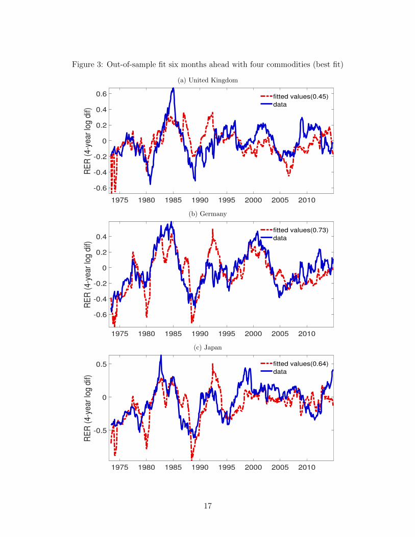
Figure 3: Out-of-sample fit six months ahead with four commodities (best fit)

(a) United Kingdom

1975 1980 1985 1990 1995 2000 2005 2010

-0.6

-0.4

-0.2

0

0.2

0.4

0.6R

ER

(4

-ye

ar

log

dif)

fitted values(0.45)

data

(b) Germany

1975 1980 1985 1990 1995 2000 2005 2010

-0.6

-0.4

-0.2

0

0.2

0.4

RE

R (

4-y

ea

r lo

g d

if)

fitted values(0.73)

data

(c) Japan

1975 1980 1985 1990 1995 2000 2005 2010

-0.5

0

0.5

RE

R (

4-y

ea

r lo

g d

if)

fitted values(0.64)

data

17

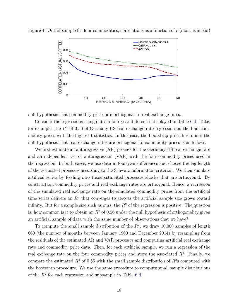
Figure 4: Out-of-sample fit, four commodities, correlations as a function of r (months ahead)

10 20 30 40 50 60

PERIODS AHEAD (MONTHS)

0

0.2

0.4

0.6

0.8

1

CO

RR

EL

AT

ION

(A

CT

UA

L V

S F

ITT

ED

)

UNITED KINGDOM

GERMANY

JAPAN

null hypothesis that commodity prices are orthogonal to real exchange rates.

Consider the regressions using data in four-year differences displayed in Table 6.d. Take,

for example, the R2 of 0.56 of Germany-US real exchange rate regression on the four com-

modity prices with the highest t-statistics. In this case, the bootstrap procedure under the

null hypothesis that real exchange rates are orthogonal to commodity prices is as follows.

We first estimate an autoregressive (AR) process for the Germany-US real exchange rate

and an independent vector autoregression (VAR) with the four commodity prices used in

the regression. In both cases, we use data in four-year differences and choose the lag length

of the estimated processes according to the Schwarz information criterion. We then simulate

artificial series by feeding into those estimated processes shocks that are orthogonal. By

construction, commodity prices and real exchange rates are orthogonal. Hence, a regression

of the simulated real exchange rate on the simulated commodity prices from the artificial

time series delivers an R2 that converges to zero as the artificial sample size grows toward

infinity. But for a sample size such as ours, the R2 of the regression is positive. The question

is, how common is it to obtain an R2 of 0.56 under the null hypothesis of orthogonality given

an artificial sample of data with the same number of observations that we have?

To compute the small sample distribution of the R2, we draw 10,000 samples of length

660 (the number of months between January 1960 and December 2014) by resampling from

the residuals of the estimated AR and VAR processes and computing artificial real exchange

rate and commodity price data. Then, for each artificial sample, we run a regression of the

real exchange rate on the four commodity prices and store the associated R2. Finally, we

compare the estimated R2 of 0.56 with the small sample distribution of R2s computed with

the bootstrap procedure. We use the same procedure to compute small sample distributions

of the R2 for each regression and subsample in Table 6.d.

18

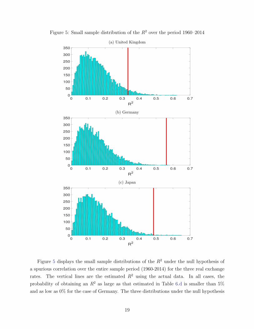
Figure 5: Small sample distribution of the R2 over the period 1960–2014

(a) United Kingdom

0 0.1 0.2 0.3 0.4 0.5 0.6 0.7

R2

0

50

100

150

200

250

300

350

(b) Germany

0 0.1 0.2 0.3 0.4 0.5 0.6 0.7

R2

0

50

100

150

200

250

300

350

(c) Japan

0 0.1 0.2 0.3 0.4 0.5 0.6 0.7

R2

0

50

100

150

200

250

300

350

Figure 5 displays the small sample distributions of the R2 under the null hypothesis of

a spurious correlation over the entire sample period (1960-2014) for the three real exchange

rates. The vertical lines are the estimated R2 using the actual data. In all cases, the

probability of obtaining an R2 as large as that estimated in Table 6.d is smaller than 5%

and as low as 0% for the case of Germany. The three distributions under the null hypothesis

19

are positively skewed with a mode of about 0.1, which is much smaller than the estimated

R2 in the table.

Table 8: Bootstrap distributions of R2 under the null hypothesis of orthogonality, with fourcommodities (best fit) in four-year differences

Percentiles distribution of R2

R2 Median 75 90 95 Pr(R2 ≥ R2)

United Kingdom1960-2014 0.33 0.13 0.20 0.27 0.31 0.0371960-1972 0.72 0.52 0.66 0.75 0.80 0.1431973-1985 0.82 0.37 0.52 0.64 0.70 0.0041986-1998 0.63 0.37 0.50 0.61 0.67 0.0771999-2014 0.58 0.29 0.41 0.53 0.59 0.059

Germany1960-2014 0.56 0.13 0.19 0.26 0.31 0.0001960-1972 0.84 0.56 0.69 0.79 0.83 0.0321973-1985 0.87 0.49 0.63 0.73 0.78 0.0051986-1998 0.81 0.40 0.54 0.65 0.71 0.0071999-2014 0.74 0.30 0.43 0.55 0.61 0.007

Japan1960-2014 0.48 0.14 0.21 0.29 0.34 0.0031960-1972 0.88 0.59 0.72 0.81 0.85 0.0221973-1985 0.76 0.46 0.60 0.70 0.75 0.0451986-1998 0.86 0.41 0.55 0.66 0.71 0.0011999-2014 0.80 0.33 0.46 0.57 0.63 0.002

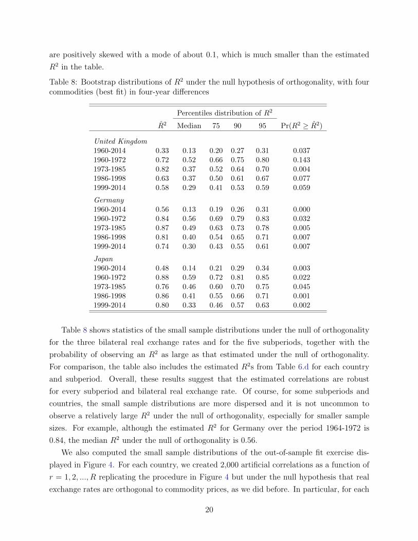
Table 8 shows statistics of the small sample distributions under the null of orthogonality

for the three bilateral real exchange rates and for the five subperiods, together with the

probability of observing an R2 as large as that estimated under the null of orthogonality.

For comparison, the table also includes the estimated R2s from Table 6.d for each country

and subperiod. Overall, these results suggest that the estimated correlations are robust

for every subperiod and bilateral real exchange rate. Of course, for some subperiods and

countries, the small sample distributions are more dispersed and it is not uncommon to

observe a relatively large R2 under the null of orthogonality, especially for smaller sample

sizes. For example, although the estimated R2 for Germany over the period 1964-1972 is

0.84, the median R2 under the null of orthogonality is 0.56.

We also computed the small sample distributions of the out-of-sample fit exercise dis-

played in Figure 4. For each country, we created 2,000 artificial correlations as a function of

r = 1, 2, ..., R replicating the procedure in Figure 4 but under the null hypothesis that real

exchange rates are orthogonal to commodity prices, as we did before. In particular, for each

20

expanding subsample (beginning with the period 1960-1972), we estimate an AR process for

the real exchange rate and a VAR process for the 10 commodities independent of the autore-

gressive process for the real exchange rate. We simulate a history of commodity prices and

real exchange rates of the appropriate size and run a regression of the real exchange rate on

the commodity prices in four-year differences. We keep the four commodities with the high-

est t-statistics and rerun the regression. With these commodities and estimated coefficients,

we perform the same out-of-sample fit that we did above over the following r = 1, 2, ..., R

periods and store the fitted values. We next expand the sample by adding one observation

and redo the entire estimation and out-of-sample fit procedure until we use all the available

data. Then we compute the correlation of the real exchange rates with their out-of-sample

fitted counterparts using the artificial time series. We repeat this procedure 2,000 times and

compute a small sample distribution of out-of-sample correlations under the null hypothesis

of orthogonality.

Figure 6 displays the median correlation for each country under the null hypothesis

(solid line), and the shaded areas represent the 5th and 95th percentiles of the small sample

distribution of the correlation as a function of the horizon r = 1, 2, ..., R. We also include in

the plot the correlation that we estimated above in Figure 4 (dashed lines). In all the cases,

we comfortably reject the null hypothesis of orthogonality.

5 The model

In this section, we present a model that, in equilibrium, delivers a system of equations

as in (2). We go into detail, since we want to consider an economy with an input-output

matrix that is slightly more complicated than the ones typically used in macro-trade models,

so as to explicitly discuss the role of prices of primary commodities, such as oil and wheat,

on final goods price indexes.

The discussion is made in the context of a simple Ricardian model, where trade is the

result of differences in endowments and productivities. We will not characterize all the equi-

librium conditions; rather, we emphasize how final good prices (and therefore real exchange

rates) are related to prices of these primary commodities in a competitive equilibrium. Since

we want to allow for heterogeneity in labor types and in differentiated intermediate goods,

the notation is rather heavy, but the ideas are very simple and well known. The analysis

also highlights under which conditions one should expect the PCP to be related to the real

exchange rate. We would like to emphasize at the outset that we will derive a relationship

between prices, all of them endogenous variables.

Specifically, we consider a world with a finite number of countries, each one inhabited

21

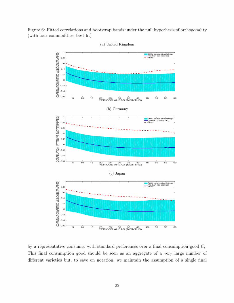
Figure 6: Fitted correlations and bootstrap bands under the null hypothesis of orthogonality(with four commodities, best fit)

(a) United Kingdom

PERIODS AHEAD (MONTHS)5 10 15 20 25 30 35 40 45 50 55 60

CORR

ELAT

ION

(FIT

TED

VS B

OO

TSTR

APPE

D)

-0.6

-0.4

-0.2

0

0.2

0.4

0.6

0.8

190% bands (bootstrap)median (bootstrap)fitted

(b) Germany


CORR

ELAT

ION

(FIT

TED

VS B

OO

TSTR

APPE

D)

-0.6

-0.4

-0.2

0

0.2

0.4

0.6

0.8


(c) Japan


CORR

ELAT

ION

(FIT

TED

VS B

OO

TSTR

APPE

D)

-0.6

-0.4

-0.2

0

0.2

0.4

0.6

0.8


by a representative consumer with standard preferences over a final consumption good Ct.

This final consumption good should be seen as an aggregate of a very large number of

different varieties but, to save on notation, we maintain the assumption of a single final

22

good.20 We assume the final good to be nontraded in order to make the model consistent

with the overwhelming evidence of the lack of a law of one price in final goods (Engel,

1999). In this sense, the model below adopts the view of Burstein et. al (2003), who argue

that an important share of final good prices have a nontraded component. To motivate

nominal magnitudes in each country, we assume that a cash-in-advance constraint of the

form PtCt ≤Mt is imposed on the representative consumer, where Pt is the price of the final

good and Mt is the quantity of money.

We will not characterize equilibrium conditions for the household, since all we will ex-

ploit is the production structure of the economy. The preferences and the cash-in-advance

constraint should be kept in the background for completeness in terms of thinking about

how quantities and nominal prices are determined in an equilibrium.

In each country, there are different varieties of labor, intermediate goods, and commodi-

ties. In particular, we assume that there are

j = 1, 2, ..., J types of labor

i = 1, 2, ..., N types of intermediate goods

h = 1, 2, ..., H types of commodities.

For simplicity, we assume that all varieties will be produced in each country. If not, the

discussion below should consider the possibility that some varieties may not be produced

in some countries, making the notation (yet) more cumbersome. This assumption does not

affect the result, as will become apparent. We also assume that for each commodity, there

is a nontradable fixed factor Et(h) for all h, which is used in the production of the primary

commodities.21 We imagine that the number of labor varieties and intermediate goods is very

large, in the order of thousands. In contrast, in the empirical section, we focused attention

on a handful (four) of primary commodities.

All technologies are assumed Cobb-Douglas, even though this assumption implies the

unrealistic restriction that sector shares are constant over time.22 Still, it makes the algebra

very simple and the expressions easy to interpret. The theoretical equation implied by this

assumption is linear in logs with parameters that are time invariant, so it naturally leads

to an equation that can be used in the empirical analysis using the simplest techniques. In

Appendix G we show that the relationship between the RER and commodity prices that we

20In Appendix H, we show how the model naturally extends to a continuum of nontraded final goods.21For instance, in the case of oil, the oil fields are non-tradable; the oil extracted using the oil fields and

other inputs is. In the case of wheat, the grain is tradable, the land used to produce it is not.22For instance, in the United States between 1960 and 2000, the service sector grew from roughly 50% of

GDP to 65%, while manufacturing dropped from 25% to 15% of GDP.

23

derived also holds for general constant returns to scale production functions, but it will not

be log-linear.

In what follows, we describe in detail the production structure of one of the economies.

To fix ideas, consider the economy whose currency is used for international transactions:

the United States in our empirical application. We now describe the environment in this

economy without any country-specific index. Those indexes will be introduced when we

consider two countries and construct a measure of their bilateral real exchange rates.

Countries may differ in their endowments of labor, nt(j) for all j, endowments of primary

commodities fixed factors, Et(h) for all h, and in the parameters of their production function,

including the total factor productivity associated with each production function. The fixed

factors used in the production of commodities and the different varieties of labor are non-

traded, while commodities are internationally traded in perfectly competitive markets. For

the expressions that we derive below, we do not need to take a stand on how tradable the

intermediate goods are.

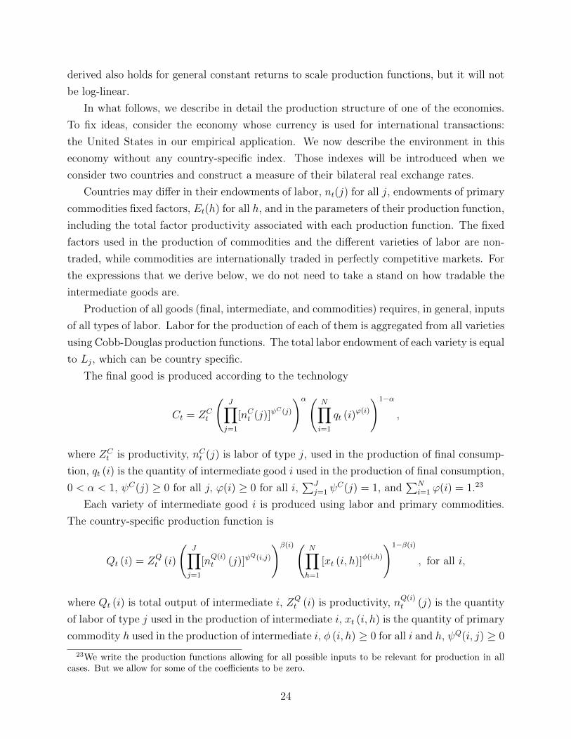
Production of all goods (final, intermediate, and commodities) requires, in general, inputs

of all types of labor. Labor for the production of each of them is aggregated from all varieties

using Cobb-Douglas production functions. The total labor endowment of each variety is equal

to Lj, which can be country specific.

The final good is produced according to the technology

Ct = ZCt

(J∏j=1

[nCt (j)]ψC(j)

)α( N∏i=1

qt (i)ϕ(i))1−α

,

where ZCt is productivity, nCt (j) is labor of type j, used in the production of final consump-

tion, qt (i) is the quantity of intermediate good i used in the production of final consumption,

0 < α < 1, ψC(j) ≥ 0 for all j, ϕ(i) ≥ 0 for all i,∑J

j=1 ψC(j) = 1, and

∑Ni=1 ϕ(i) = 1.23

Each variety of intermediate good i is produced using labor and primary commodities.

The country-specific production function is

Qt (i) = ZQt (i)

(J∏j=1

[nQ(i)t (j)]ψ

Q(i,j)

)β(i)( N∏h=1

[xt (i, h)]φ(i,h))1−β(i)

, for all i,

where Qt (i) is total output of intermediate i, ZQt (i) is productivity, n

Q(i)t (j) is the quantity

of labor of type j used in the production of intermediate i, xt (i, h) is the quantity of primary

commodity h used in the production of intermediate i, φ (i, h) ≥ 0 for all i and h, ψQ(i, j) ≥ 0

23We write the production functions allowing for all possible inputs to be relevant for production in allcases. But we allow for some of the coefficients to be zero.

24

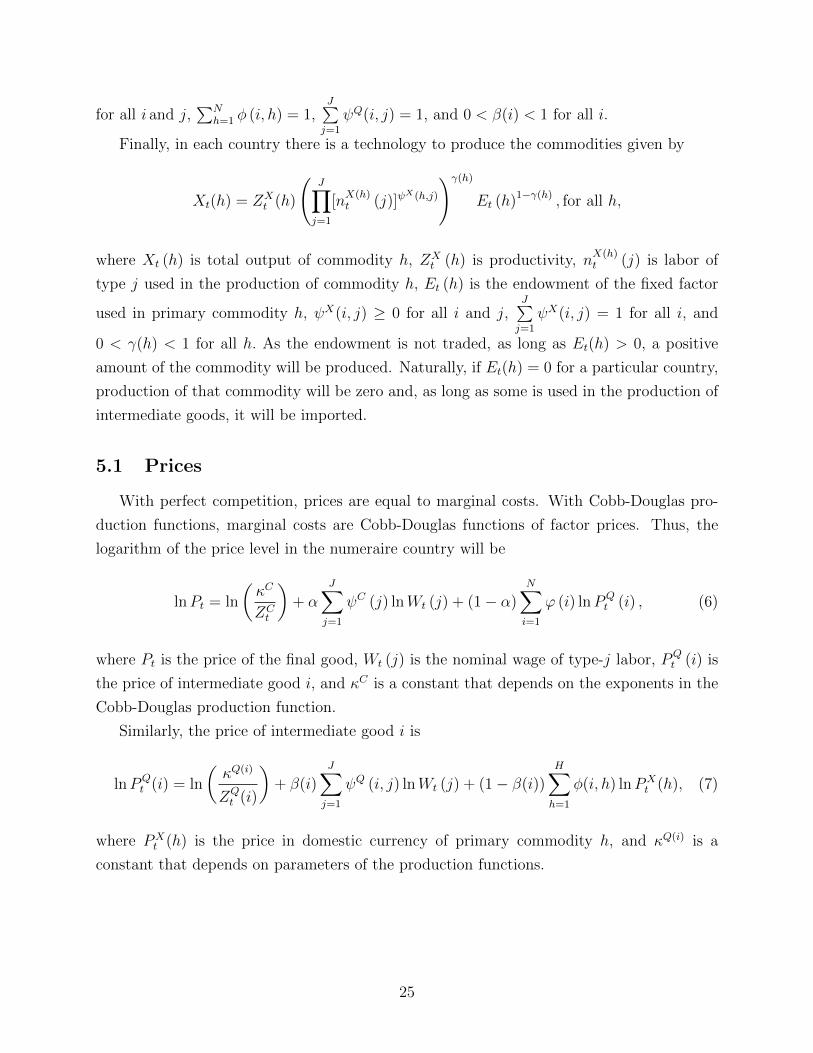
for all i and j,∑N

h=1 φ (i, h) = 1,J∑j=1

ψQ(i, j) = 1, and 0 < β(i) < 1 for all i.

Finally, in each country there is a technology to produce the commodities given by

Xt(h) = ZXt (h)

(J∏j=1

[nX(h)t (j)]ψ

X(h,j)

)γ(h)

Et (h)1−γ(h) , for all h,

where Xt (h) is total output of commodity h, ZXt (h) is productivity, n

X(h)t (j) is labor of

type j used in the production of commodity h, Et (h) is the endowment of the fixed factor

used in primary commodity h, ψX(i, j) ≥ 0 for all i and j,J∑j=1

ψX(i, j) = 1 for all i, and

0 < γ(h) < 1 for all h. As the endowment is not traded, as long as Et(h) > 0, a positive

amount of the commodity will be produced. Naturally, if Et(h) = 0 for a particular country,

production of that commodity will be zero and, as long as some is used in the production of

intermediate goods, it will be imported.

5.1 Prices

With perfect competition, prices are equal to marginal costs. With Cobb-Douglas pro-

duction functions, marginal costs are Cobb-Douglas functions of factor prices. Thus, the

logarithm of the price level in the numeraire country will be

lnPt = ln

(κC

ZCt

)+ α

J∑j=1

ψC (j) lnWt (j) + (1− α)N∑i=1

ϕ (i) lnPQt (i) , (6)

where Pt is the price of the final good, Wt (j) is the nominal wage of type-j labor, PQt (i) is

the price of intermediate good i, and κC is a constant that depends on the exponents in the

Cobb-Douglas production function.

Similarly, the price of intermediate good i is

lnPQt (i) = ln

(κQ(i)

ZQt (i)

)+ β(i)

J∑j=1

ψQ (i, j) lnWt (j) + (1− β(i))H∑h=1

φ(i, h) lnPXt (h), (7)

where PXt (h) is the price in domestic currency of primary commodity h, and κQ(i) is a

constant that depends on parameters of the production functions.

25

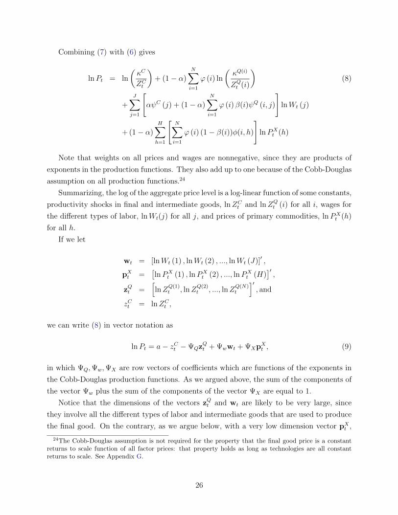
Combining (7) with (6) gives

lnPt = ln

(κC

ZCt

)+ (1− α)

N∑i=1

ϕ (i) ln

(κQ(i)

ZQt (i)

)(8)

+J∑j=1

[αψC (j) + (1− α)

N∑i=1

ϕ (i) β(i)ψQ (i, j)

]lnWt (j)

+ (1− α)H∑h=1

[N∑i=1

ϕ (i) (1− β(i))φ(i, h)

]lnPX

t (h)

Note that weights on all prices and wages are nonnegative, since they are products of

exponents in the production functions. They also add up to one because of the Cobb-Douglas

assumption on all production functions.24

Summarizing, the log of the aggregate price level is a log-linear function of some constants,

productivity shocks in final and intermediate goods, lnZCt and lnZQ

t (i) for all i, wages for

the different types of labor, lnWt(j) for all j, and prices of primary commodities, lnPXt (h)

for all h.

If we let

wt = [lnWt (1) , lnWt (2) , ..., lnWt (J)]′ ,

pXt =[lnPX

t (1) , lnPXt (2) , ..., lnPX

t (H)]′,

zQt =[lnZ

Q(1)t , lnZ

Q(2)t , ..., lnZ

Q(N)t

]′, and

zCt = lnZCt ,

we can write (8) in vector notation as

lnPt = a− zCt −ΨQzQt + Ψwwt + ΨXpXt , (9)

in which ΨQ,Ψw,ΨX are row vectors of coefficients which are functions of the exponents in

the Cobb-Douglas production functions. As we argued above, the sum of the components of

the vector Ψw plus the sum of the components of the vector ΨX are equal to 1.

Notice that the dimensions of the vectors zQt and wt are likely to be very large, since

they involve all the different types of labor and intermediate goods that are used to produce

the final good. On the contrary, as we argue below, with a very low dimension vector pXt ,

24The Cobb-Douglas assumption is not required for the property that the final good price is a constantreturns to scale function of all factor prices: that property holds as long as technologies are all constantreturns to scale. See Appendix G.

26

one can go a long way in accounting for real exchange rate variability.

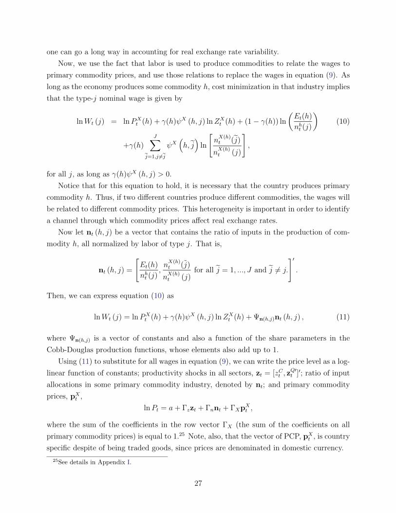
Now, we use the fact that labor is used to produce commodities to relate the wages to

primary commodity prices, and use those relations to replace the wages in equation (9). As

long as the economy produces some commodity h, cost minimization in that industry implies

that the type-j nominal wage is given by

lnWt (j) = lnPXt (h) + γ(h)ψX (h, j) lnZX

t (h) + (1− γ(h)) ln

(Et(h)

nht (j)

)(10)

+γ(h)J∑

j=1,j 6=j

ψX(h, j)

ln

[nX(h)t (j)

nX(h)t (j)

],

for all j, as long as γ(h)ψX (h, j) > 0.

Notice that for this equation to hold, it is necessary that the country produces primary

commodity h. Thus, if two different countries produce different commodities, the wages will

be related to different commodity prices. This heterogeneity is important in order to identify

a channel through which commodity prices affect real exchange rates.

Now let nt (h, j) be a vector that contains the ratio of inputs in the production of com-

modity h, all normalized by labor of type j. That is,

nt (h, j) =

[Et(h)

nht (j),nX(h)t (j)

nX(h)t (j)

for all j = 1, ..., J and j 6= j.

]′.

Then, we can express equation (10) as

lnWt (j) = lnPXt (h) + γ(h)ψX (h, j) lnZX

t (h) + Ψn(h,j)nt (h, j) , (11)

where Ψn(h,j) is a vector of constants and also a function of the share parameters in the

Cobb-Douglas production functions, whose elements also add up to 1.

Using (11) to substitute for all wages in equation (9), we can write the price level as a log-

linear function of constants; productivity shocks in all sectors, zt = [zCt , zQ′t ]′; ratio of input

allocations in some primary commodity industry, denoted by nt; and primary commodity

prices, pXt ,

lnPt = a+ Γzzt + Γnnt + ΓXpXt ,

where the sum of the coefficients in the row vector ΓX (the sum of the coefficients on all

primary commodity prices) is equal to 1.25 Note, also, that the vector of PCP, pXt , is country

specific despite of being traded goods, since prices are denominated in domestic currency.

25See details in Appendix I.

27

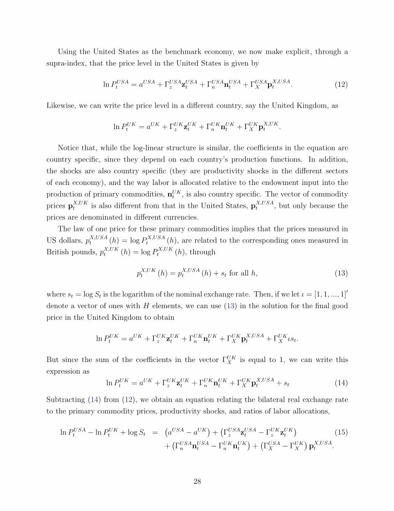
Using the United States as the benchmark economy, we now make explicit, through a

supra-index, that the price level in the United States is given by

lnPUSAt = aUSA + ΓUSAz zUSAt + ΓUSAn nUSAt + ΓUSAX pX,USAt . (12)

Likewise, we can write the price level in a different country, say the United Kingdom, as

lnPUKt = aUK + ΓUKz zUKt + ΓUKn nUKt + ΓUKX pX,UKt .

Notice that, while the log-linear structure is similar, the coefficients in the equation are

country specific, since they depend on each country’s production functions. In addition,

the shocks are also country specific (they are productivity shocks in the different sectors

of each economy), and the way labor is allocated relative to the endowment input into the

production of primary commodities, nUKt , is also country specific. The vector of commodity

prices pX,UKt is also different from that in the United States, pX,USAt , but only because the

prices are denominated in different currencies.

The law of one price for these primary commodities implies that the prices measured in

US dollars, pX,USAt (h) = logPX,USAt (h), are related to the corresponding ones measured in

British pounds, pX,UKt (h) = logPX,UKt (h), through

pX,UKt (h) = pX,USAt (h) + st for all h, (13)

where st = logSt is the logarithm of the nominal exchange rate. Then, if we let ι = [1, 1, ..., 1]′

denote a vector of ones with H elements, we can use (13) in the solution for the final good

price in the United Kingdom to obtain

lnPUKt = aUK + ΓUKz zUKt + ΓUKn nUKt + ΓUKX pX,USAt + ΓUKX ιst.

But since the sum of the coefficients in the vector ΓUKX is equal to 1, we can write this

expression as

lnPUKt = aUK + ΓUKz zUKt + ΓUKn nUKt + ΓUKX pX,USAt + st (14)

Subtracting (14) from (12), we obtain an equation relating the bilateral real exchange rate

to the primary commodity prices, productivity shocks, and ratios of labor allocations,

lnPUSAt − lnPUK

t + logSt =(aUSA − aUK

)+(ΓUSAz zUSAt − ΓUKz zUKt

)(15)

+(ΓUSAn nUSAt − ΓUKn nUKt

)+(ΓUSAX − ΓUKX

)pX,USAt .

28

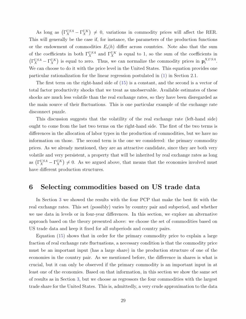
As long as(ΓUSAX − ΓUKX

)6= 0, variations in commodity prices will affect the RER.

This will generally be the case if, for instance, the parameters of the production functions

or the endowment of commodities Et(h) differ across countries. Note also that the sum

of the coefficients in both ΓUSAX and ΓUKX is equal to 1, so the sum of the coefficients in(ΓUSAX − ΓUKX

)is equal to zero. Thus, we can normalize the commodity prices in pX,USAt .

We can choose to do it with the price level in the United States. This equation provides one

particular rationalization for the linear regression postulated in (1) in Section 2.1.

The first term on the right-hand side of (15) is a constant, and the second is a vector of

total factor productivity shocks that we treat as unobservable. Available estimates of these

shocks are much less volatile than the real exchange rates, so they have been disregarded as

the main source of their fluctuations. This is one particular example of the exchange rate

disconnect puzzle.

This discussion suggests that the volatility of the real exchange rate (left-hand side)

ought to come from the last two terms on the right-hand side. The first of the two terms is

differences in the allocation of labor types in the production of commodities, but we have no

information on those. The second term is the one we considered: the primary commodity

prices. As we already mentioned, they are an attractive candidate, since they are both very

volatile and very persistent, a property that will be inherited by real exchange rates as long

as(ΓUSAX − ΓUKX

)6= 0. As we argued above, that means that the economies involved must

have different production structures.

6 Selecting commodities based on US trade data

In Section 3 we showed the results with the four PCP that make the best fit with the

real exchange rates. This set (possibly) varies by country pair and subperiod, and whether

we use data in levels or in four-year differences. In this section, we explore an alternative

approach based on the theory presented above: we choose the set of commodities based on

US trade data and keep it fixed for all subperiods and country pairs.

Equation (15) shows that in order for the primary commodity price to explain a large

fraction of real exchange rate fluctuations, a necessary condition is that the commodity price

must be an important input (has a large share) in the production structure of one of the

economies in the country pair. As we mentioned before, the difference in shares is what is

crucial, but it can only be observed if the primary commodity is an important input in at

least one of the economies. Based on that information, in this section we show the same set

of results as in Section 3, but we choose as regressors the four commodities with the largest

trade share for the United States. This is, admittedly, a very crude approximation to the data

29

using the model of the previous section, but it has the advantage that the four commodities

have not been chosen to fit the data. We see this exercise as a first approximation to using

the model to discipline our choices in the empirical analysis.

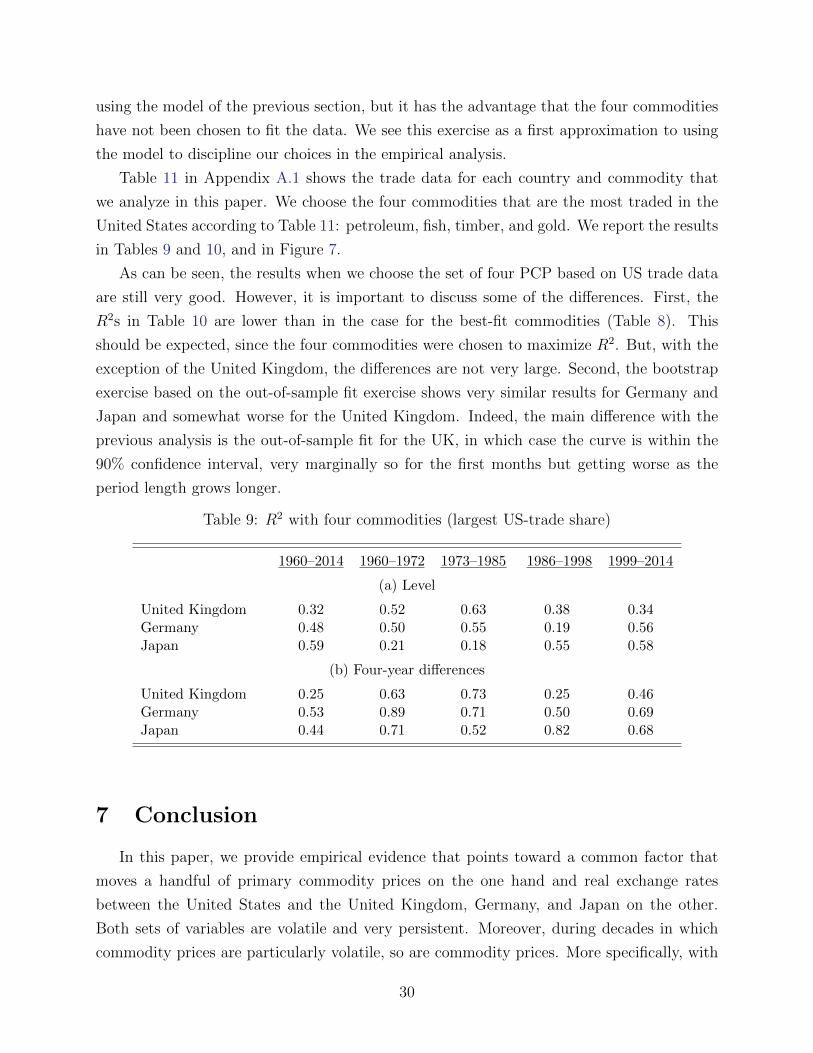
Table 11 in Appendix A.1 shows the trade data for each country and commodity that

we analyze in this paper. We choose the four commodities that are the most traded in the

United States according to Table 11: petroleum, fish, timber, and gold. We report the results

in Tables 9 and 10, and in Figure 7.

As can be seen, the results when we choose the set of four PCP based on US trade data

are still very good. However, it is important to discuss some of the differences. First, the

R2s in Table 10 are lower than in the case for the best-fit commodities (Table 8). This

should be expected, since the four commodities were chosen to maximize R2. But, with the

exception of the United Kingdom, the differences are not very large. Second, the bootstrap

exercise based on the out-of-sample fit exercise shows very similar results for Germany and

Japan and somewhat worse for the United Kingdom. Indeed, the main difference with the

previous analysis is the out-of-sample fit for the UK, in which case the curve is within the

90% confidence interval, very marginally so for the first months but getting worse as the

period length grows longer.

Table 9: R2 with four commodities (largest US-trade share)

1960–2014 1960–1972 1973–1985 1986–1998 1999–2014

(a) Level




7 Conclusion

In this paper, we provide empirical evidence that points toward a common factor that

moves a handful of primary commodity prices on the one hand and real exchange rates

between the United States and the United Kingdom, Germany, and Japan on the other.

Both sets of variables are volatile and very persistent. Moreover, during decades in which

commodity prices are particularly volatile, so are commodity prices. More specifically, with

30

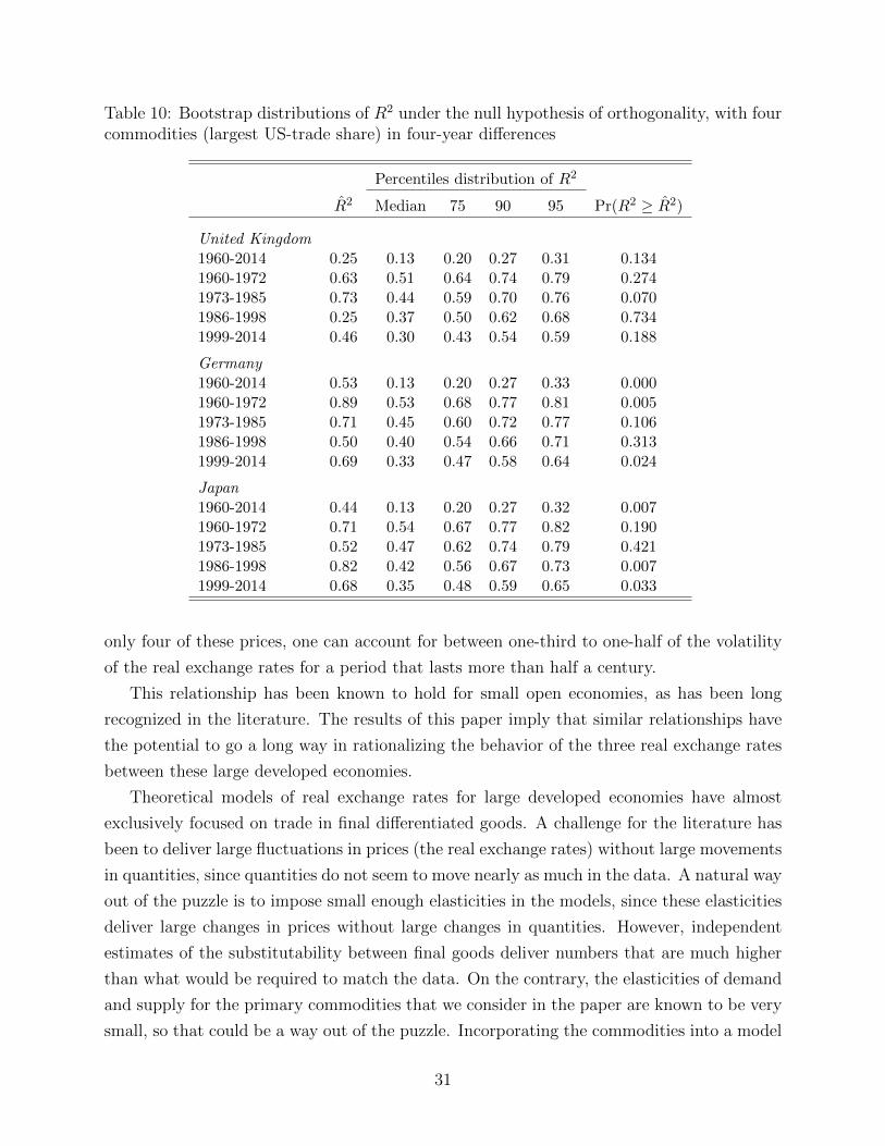
Table 10: Bootstrap distributions of R2 under the null hypothesis of orthogonality, with fourcommodities (largest US-trade share) in four-year differences


R2 Median 75 90 95 Pr(R2 ≥ R2)

United Kingdom1960-2014 0.25 0.13 0.20 0.27 0.31 0.1341960-1972 0.63 0.51 0.64 0.74 0.79 0.2741973-1985 0.73 0.44 0.59 0.70 0.76 0.0701986-1998 0.25 0.37 0.50 0.62 0.68 0.7341999-2014 0.46 0.30 0.43 0.54 0.59 0.188

Germany1960-2014 0.53 0.13 0.20 0.27 0.33 0.0001960-1972 0.89 0.53 0.68 0.77 0.81 0.0051973-1985 0.71 0.45 0.60 0.72 0.77 0.1061986-1998 0.50 0.40 0.54 0.66 0.71 0.3131999-2014 0.69 0.33 0.47 0.58 0.64 0.024

Japan1960-2014 0.44 0.13 0.20 0.27 0.32 0.0071960-1972 0.71 0.54 0.67 0.77 0.82 0.1901973-1985 0.52 0.47 0.62 0.74 0.79 0.4211986-1998 0.82 0.42 0.56 0.67 0.73 0.0071999-2014 0.68 0.35 0.48 0.59 0.65 0.033

only four of these prices, one can account for between one-third to one-half of the volatility

of the real exchange rates for a period that lasts more than half a century.

This relationship has been known to hold for small open economies, as has been long

recognized in the literature. The results of this paper imply that similar relationships have

the potential to go a long way in rationalizing the behavior of the three real exchange rates

between these large developed economies.

Theoretical models of real exchange rates for large developed economies have almost

exclusively focused on trade in final differentiated goods. A challenge for the literature has

been to deliver large fluctuations in prices (the real exchange rates) without large movements

in quantities, since quantities do not seem to move nearly as much in the data. A natural way

out of the puzzle is to impose small enough elasticities in the models, since these elasticities

deliver large changes in prices without large changes in quantities. However, independent

estimates of the substitutability between final goods deliver numbers that are much higher

than what would be required to match the data. On the contrary, the elasticities of demand

and supply for the primary commodities that we consider in the paper are known to be very

small, so that could be a way out of the puzzle. Incorporating the commodities into a model

31

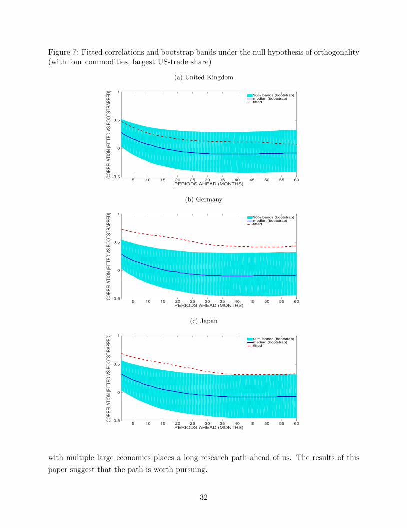
Figure 7: Fitted correlations and bootstrap bands under the null hypothesis of orthogonality(with four commodities, largest US-trade share)

(a) United Kingdom


CO

RR

ELA

TIO

N (F

ITTE

D V

S B

OO

TSTR

AP

PE

D)

-0.5

0

0.5


(b) Germany


CO

RR

ELA

TIO

N (F

ITTE

D V

S B

OO

TSTR

AP

PE

D)

-0.5

0

0.5


(c) Japan


CO

RR

ELA

TIO

N (F

ITTE

D V

S B

OO

TSTR

AP

PE

D)

-0.5

0

0.5


with multiple large economies places a long research path ahead of us. The results of this

paper suggest that the path is worth pursuing.

32

References

[1] Betts, C. M. and T. J. Kehoe. “U.S. Real Exchange Rate Fluctuations and Relative

Price Fluctuations,” Staff Report 334, Federal Reserve Bank of Minneapolis (2004).

[2] Burstein, A. T., J. C. Neves, and S. Rebelo. “Distribution Costs and Real Exchange

Rate Dynamics During Exchange-Rate-Based Stabilizations,” Journal of Monetary Eco-

nomics, 50(6), 1189-1214 (2003).

[3] Chari, V.V., P. J. Kehoe and E. R. McGrattan. “Can Sticky Price Models Generate

Volatile and Persistent Real Exchange Rates?,” Review of Economic Studies, 69(3),

533-563 (2002).

[4] Chen, Y.-C. and K. Rogoff. “Commodity Currencies,” Journal of International Eco-

nomics, 60(1), 133-160 (2003).

[5] Eaton, J., B. Neiman, and S. Kortum. “Obstfeld and Rogoff’s International Macro

Puzzles: A Quantitative Assessment,” Journal of Economic Dynamics and Control,

72(C), 5-23 (2016).

[6] Engel, C. “Accounting for U.S. Real Exchange Rate Changes,” Journal of Political

Economy, 107(3), 507-538 (1999).

[7] Hevia, C. and J. P. Nicolini. “Optimal Devaluations,” IMF Economic Review, 61(1),

22-51 (2013).

[8] Itskhoki, O. and D. Mukhin. “Exchange Rate Disconnect in General Equilibrium,”

Working Paper, Princeton University (2017).

[9] Johansen, S. “Estimation and Hypothesis Testing of Cointegration Vectors in Gaussian

Vector Autoregressive Models,” Econometrica, 59(6), 1551-1580 (1991).

[10] Meese, R. A. and K. Rogoff. “Empirical Exchange Rate Models of the Seventies: Do

They Fit Out of Sample?,” Journal of International Economics, 14(1-2), 3-24 (1983).

[11] Mussa, M. “Nominal Exchange Rate Regimes and the Behavior of Real Exchange Rates:

Evidence and Implications,” Carnegie-Rochester Conference Series on Public Policy,

25(1), 117-214 (1986).

[12] Obstfeld, M. and K. Rogoff. “Exchange Rate Dynamics Redux,” Journal of Political

Economy, 103(3), 624-660 (1995).

33

[13] Obstfeld, M. and K. Rogoff. “The Six Mayor Puzzels in International Macroeconomics:

Is There a Common Cause?,” in B. S. Bernanke and K. Rogoff (eds.), NBER Macroe-

conomics Annual 2000, vol. 15, pp. 339-390. Cambridge, MA: MIT Press (2001).

[14] Stock, J. H. and M. W. Watson. “A Simple Estimator of Cointegrating Vectors in Higher

Order Integrated Systems,” Econometrica, 61(4), 783-820 (1993).

34

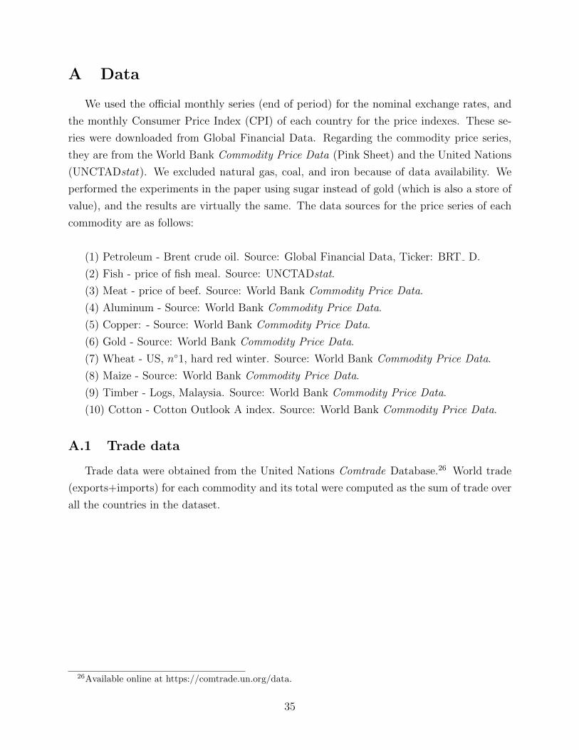
A Data

We used the official monthly series (end of period) for the nominal exchange rates, and

the monthly Consumer Price Index (CPI) of each country for the price indexes. These se-

ries were downloaded from Global Financial Data. Regarding the commodity price series,

they are from the World Bank Commodity Price Data (Pink Sheet) and the United Nations

(UNCTADstat). We excluded natural gas, coal, and iron because of data availability. We

performed the experiments in the paper using sugar instead of gold (which is also a store of

value), and the results are virtually the same. The data sources for the price series of each

commodity are as follows:

(1) Petroleum - Brent crude oil. Source: Global Financial Data, Ticker: BRT D.

(2) Fish - price of fish meal. Source: UNCTADstat.

(3) Meat - price of beef. Source: World Bank Commodity Price Data.

(4) Aluminum - Source: World Bank Commodity Price Data.

(5) Copper: - Source: World Bank Commodity Price Data.

(6) Gold - Source: World Bank Commodity Price Data.

(7) Wheat - US, n1, hard red winter. Source: World Bank Commodity Price Data.

(8) Maize - Source: World Bank Commodity Price Data.

(9) Timber - Logs, Malaysia. Source: World Bank Commodity Price Data.

(10) Cotton - Cotton Outlook A index. Source: World Bank Commodity Price Data.

A.1 Trade data

Trade data were obtained from the United Nations Comtrade Database.26 World trade

(exports+imports) for each commodity and its total were computed as the sum of trade over

all the countries in the dataset.

26Available online at https://comtrade.un.org/data.

35

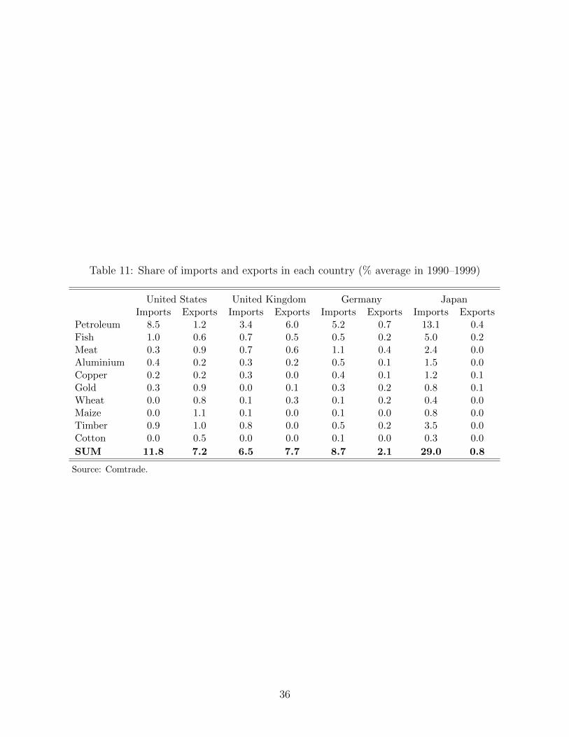
Table 11: Share of imports and exports in each country (% average in 1990–1999)

United States United Kingdom Germany JapanImports Exports Imports Exports Imports Exports Imports Exports

Petroleum 8.5 1.2 3.4 6.0 5.2 0.7 13.1 0.4Fish 1.0 0.6 0.7 0.5 0.5 0.2 5.0 0.2Meat 0.3 0.9 0.7 0.6 1.1 0.4 2.4 0.0Aluminium 0.4 0.2 0.3 0.2 0.5 0.1 1.5 0.0Copper 0.2 0.2 0.3 0.0 0.4 0.1 1.2 0.1Gold 0.3 0.9 0.0 0.1 0.3 0.2 0.8 0.1Wheat 0.0 0.8 0.1 0.3 0.1 0.2 0.4 0.0Maize 0.0 1.1 0.1 0.0 0.1 0.0 0.8 0.0Timber 0.9 1.0 0.8 0.0 0.5 0.2 3.5 0.0Cotton 0.0 0.5 0.0 0.0 0.1 0.0 0.3 0.0

SUM 11.8 7.2 6.5 7.7 8.7 2.1 29.0 0.8

Source: Comtrade.

36

ONLINE APPENDIX(not for publication)

B Real exchange rates and fitted values (level)

Figure 8: Real exchange rates and fitted values, level.

(a) United Kingdom

1965 1970 1975 1980 1985 1990 1995 2000 2005 2010

-0.1

0

0.1

0.2

0.3

0.4

0.5

RE

AL

EX

CH

AN

GE

RA

TE (L

OG

) fitted values with 10 commodities (0.71)


data

(b) Germany

1965 1970 1975 1980 1985 1990 1995 2000 2005 2010

0.3

0.4

0.5

0.6

0.7

0.8

0.9

1

RE

AL

EX

CH

AN

GE

RA

TE (L

OG



data

(c) Japan

1965 1970 1975 1980 1985 1990 1995 2000 2005 2010

0.2

0.4

0.6

0.8

1

1.2

1.4

1.6

RE

AL

EX

CH

AN

GE

RA

TE (L

OG



data

37

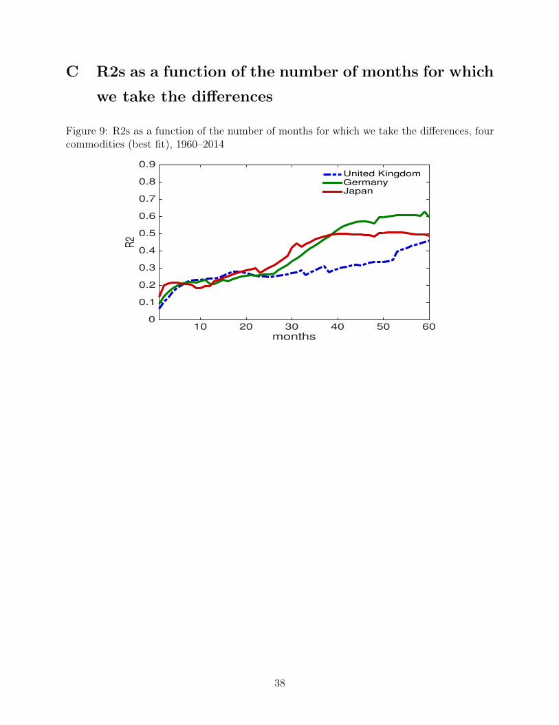
C R2s as a function of the number of months for which

we take the differences

Figure 9: R2s as a function of the number of months for which we take the differences, fourcommodities (best fit), 1960–2014

months10 20 30 40 50 60

R2

0

0.1

0.2

0.3

0.4

0.5

0.6

0.7

0.8

0.9United KingdomGermanyJapan

38

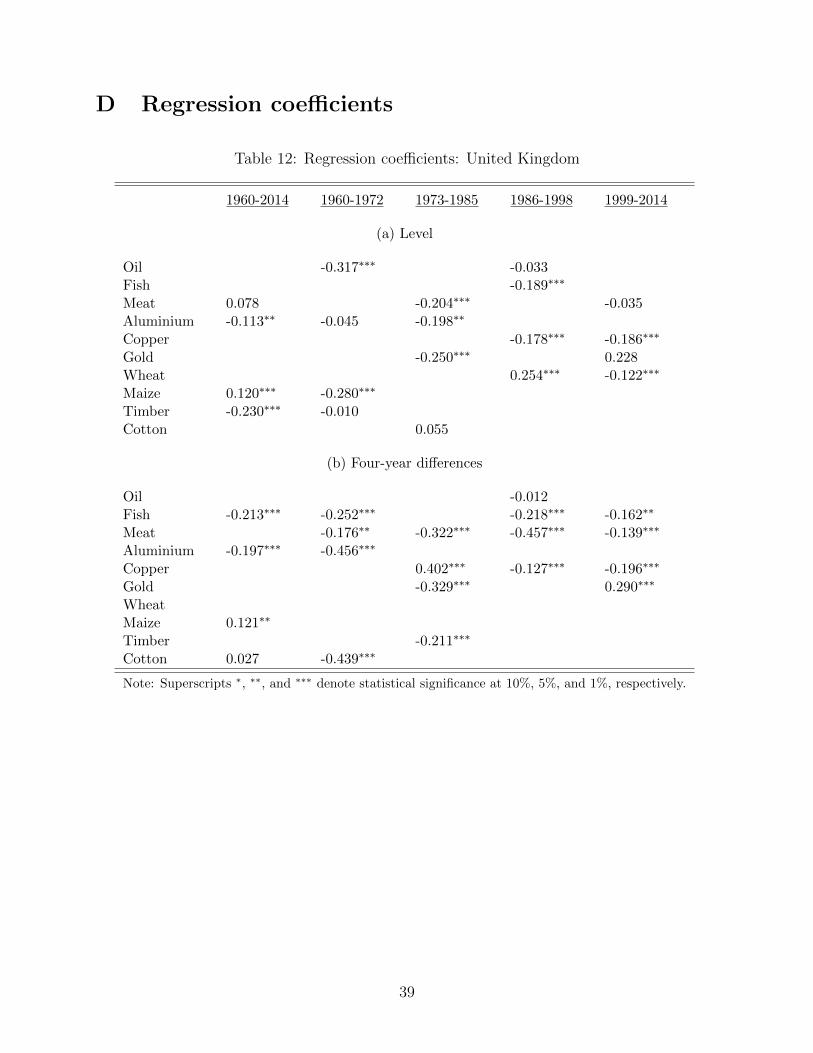
D Regression coefficients

Table 12: Regression coefficients: United Kingdom

1960-2014 1960-1972 1973-1985 1986-1998 1999-2014

(a) Level

Oil -0.317∗∗∗ -0.033Fish -0.189∗∗∗

Meat 0.078 -0.204∗∗∗ -0.035Aluminium -0.113∗∗ -0.045 -0.198∗∗

Copper -0.178∗∗∗ -0.186∗∗∗

Gold -0.250∗∗∗ 0.228Wheat 0.254∗∗∗ -0.122∗∗∗

Maize 0.120∗∗∗ -0.280∗∗∗

Timber -0.230∗∗∗ -0.010Cotton 0.055


Oil -0.012Fish -0.213∗∗∗ -0.252∗∗∗ -0.218∗∗∗ -0.162∗∗

Meat -0.176∗∗ -0.322∗∗∗ -0.457∗∗∗ -0.139∗∗∗

Aluminium -0.197∗∗∗ -0.456∗∗∗

Copper 0.402∗∗∗ -0.127∗∗∗ -0.196∗∗∗

Gold -0.329∗∗∗ 0.290∗∗∗

WheatMaize 0.121∗∗

Timber -0.211∗∗∗

Cotton 0.027 -0.439∗∗∗

Note: Superscripts ∗, ∗∗, and ∗∗∗ denote statistical significance at 10%, 5%, and 1%, respectively.

39

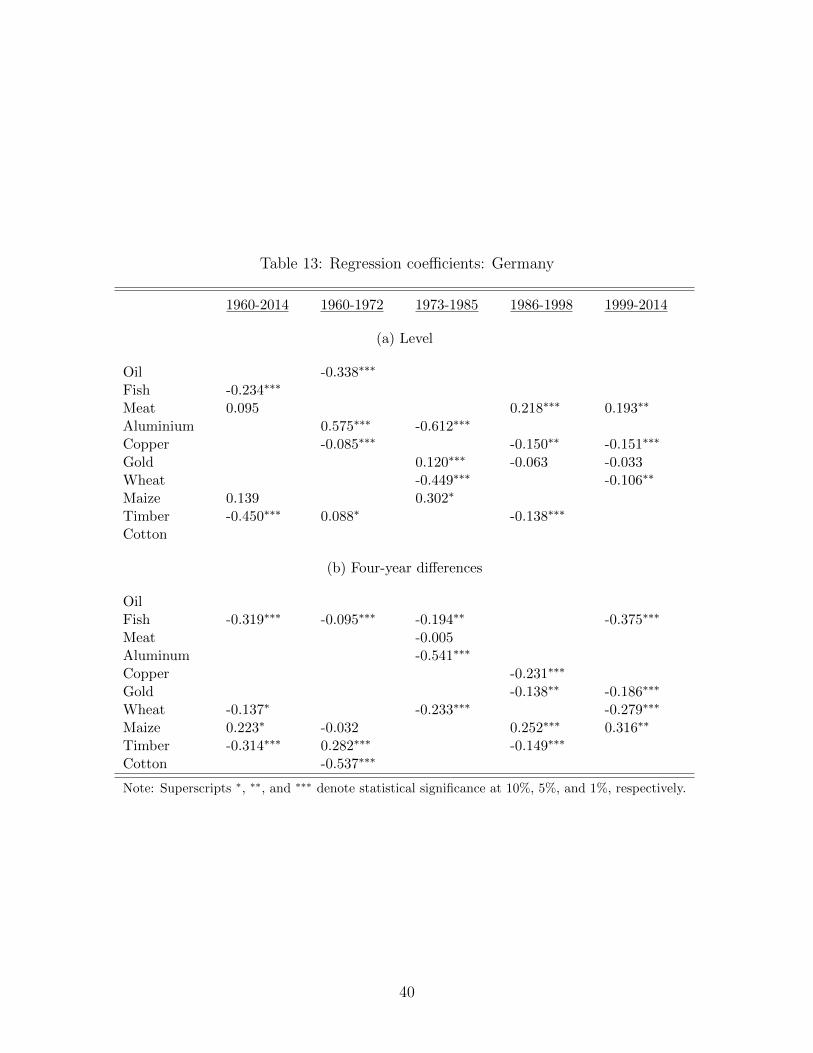
Table 13: Regression coefficients: Germany

1960-2014 1960-1972 1973-1985 1986-1998 1999-2014

(a) Level

Oil -0.338∗∗∗

Fish -0.234∗∗∗

Meat 0.095 0.218∗∗∗ 0.193∗∗

Aluminium 0.575∗∗∗ -0.612∗∗∗

Copper -0.085∗∗∗ -0.150∗∗ -0.151∗∗∗

Gold 0.120∗∗∗ -0.063 -0.033Wheat -0.449∗∗∗ -0.106∗∗

Maize 0.139 0.302∗

Timber -0.450∗∗∗ 0.088∗ -0.138∗∗∗

Cotton


OilFish -0.319∗∗∗ -0.095∗∗∗ -0.194∗∗ -0.375∗∗∗

Meat -0.005Aluminum -0.541∗∗∗

Copper -0.231∗∗∗

Gold -0.138∗∗ -0.186∗∗∗

Wheat -0.137∗ -0.233∗∗∗ -0.279∗∗∗

Maize 0.223∗ -0.032 0.252∗∗∗ 0.316∗∗

Timber -0.314∗∗∗ 0.282∗∗∗ -0.149∗∗∗

Cotton -0.537∗∗∗


40

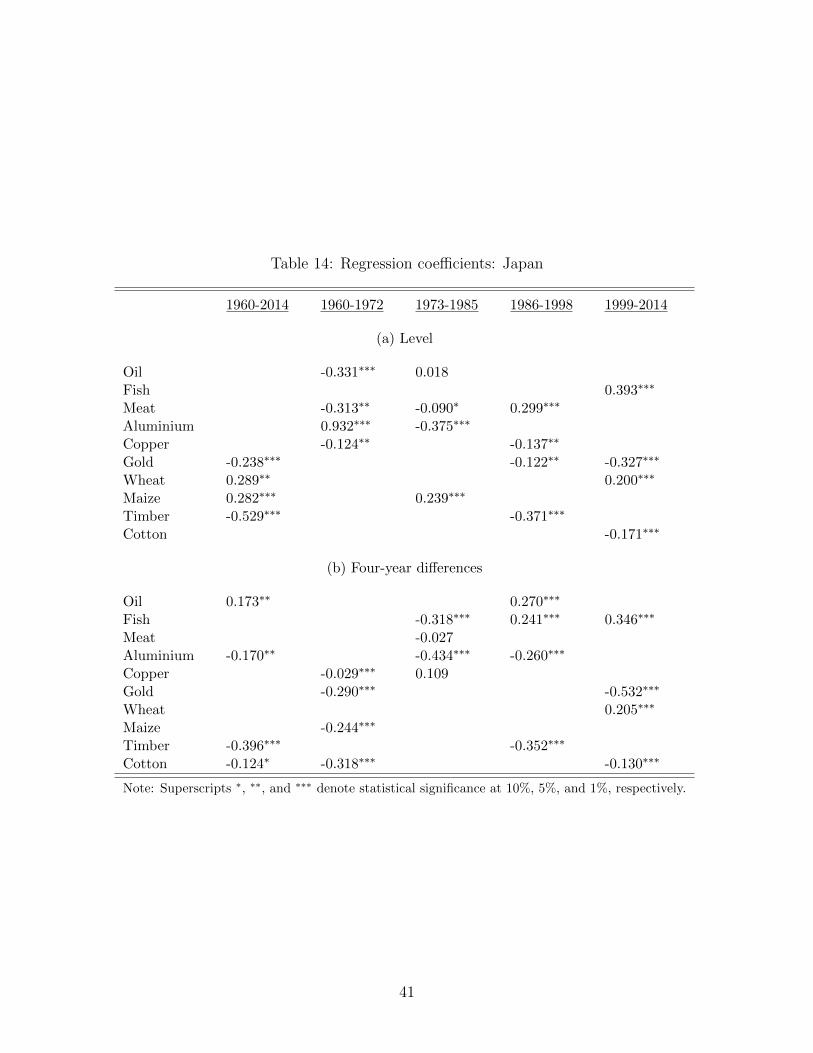
Table 14: Regression coefficients: Japan

1960-2014 1960-1972 1973-1985 1986-1998 1999-2014

(a) Level

Oil -0.331∗∗∗ 0.018Fish 0.393∗∗∗

Meat -0.313∗∗ -0.090∗ 0.299∗∗∗

Aluminium 0.932∗∗∗ -0.375∗∗∗

Copper -0.124∗∗ -0.137∗∗

Gold -0.238∗∗∗ -0.122∗∗ -0.327∗∗∗

Wheat 0.289∗∗ 0.200∗∗∗

Maize 0.282∗∗∗ 0.239∗∗∗

Timber -0.529∗∗∗ -0.371∗∗∗

Cotton -0.171∗∗∗


Oil 0.173∗∗ 0.270∗∗∗

Fish -0.318∗∗∗ 0.241∗∗∗ 0.346∗∗∗

Meat -0.027Aluminium -0.170∗∗ -0.434∗∗∗ -0.260∗∗∗

Copper -0.029∗∗∗ 0.109Gold -0.290∗∗∗ -0.532∗∗∗

Wheat 0.205∗∗∗

Maize -0.244∗∗∗

Timber -0.396∗∗∗ -0.352∗∗∗

Cotton -0.124∗ -0.318∗∗∗ -0.130∗∗∗


41

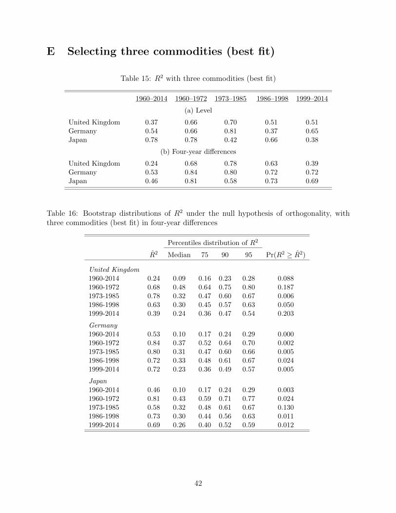
E Selecting three commodities (best fit)

Table 15: R2 with three commodities (best fit)

1960–2014 1960–1972 1973–1985 1986–1998 1999–2014

(a) Level




Table 16: Bootstrap distributions of R2 under the null hypothesis of orthogonality, withthree commodities (best fit) in four-year differences


R2 Median 75 90 95 Pr(R2 ≥ R2)

United Kingdom1960-2014 0.24 0.09 0.16 0.23 0.28 0.0881960-1972 0.68 0.48 0.64 0.75 0.80 0.1871973-1985 0.78 0.32 0.47 0.60 0.67 0.0061986-1998 0.63 0.30 0.45 0.57 0.63 0.0501999-2014 0.39 0.24 0.36 0.47 0.54 0.203

Germany1960-2014 0.53 0.10 0.17 0.24 0.29 0.0001960-1972 0.84 0.37 0.52 0.64 0.70 0.0021973-1985 0.80 0.31 0.47 0.60 0.66 0.0051986-1998 0.72 0.33 0.48 0.61 0.67 0.0241999-2014 0.72 0.23 0.36 0.49 0.57 0.005

Japan1960-2014 0.46 0.10 0.17 0.24 0.29 0.0031960-1972 0.81 0.43 0.59 0.71 0.77 0.0241973-1985 0.58 0.32 0.48 0.61 0.67 0.1301986-1998 0.73 0.30 0.44 0.56 0.63 0.0111999-2014 0.69 0.26 0.40 0.52 0.59 0.012

42

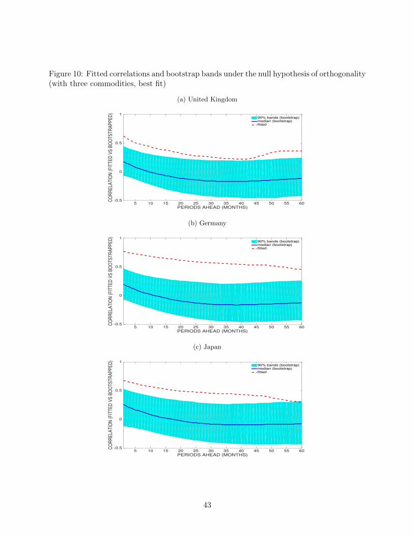
Figure 10: Fitted correlations and bootstrap bands under the null hypothesis of orthogonality(with three commodities, best fit)

(a) United Kingdom


CO

RR

ELA

TIO

N (F

ITTE

D V

S B

OO

TSTR

AP

PE

D)

-0.5

0

0.5


(b) Germany


CO

RR

ELA

TIO

N (F

ITTE

D V

S B

OO

TSTR

AP

PE

D)

-0.5

0

0.5


(c) Japan


CO

RR

ELA

TIO

N (F

ITTE

D V

S B

OO

TSTR

AP

PE

D)

-0.5

0

0.5


43

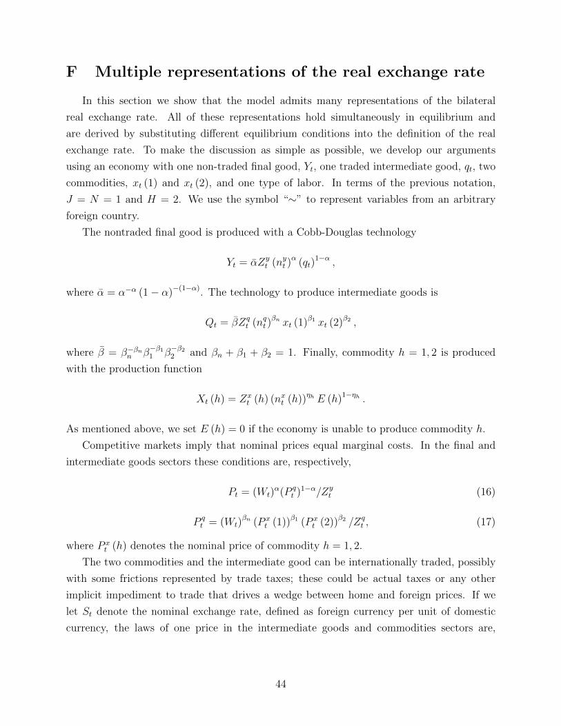
F Multiple representations of the real exchange rate

In this section we show that the model admits many representations of the bilateral

real exchange rate. All of these representations hold simultaneously in equilibrium and

are derived by substituting different equilibrium conditions into the definition of the real

exchange rate. To make the discussion as simple as possible, we develop our arguments

using an economy with one non-traded final good, Yt, one traded intermediate good, qt, two

commodities, xt (1) and xt (2), and one type of labor. In terms of the previous notation,

J = N = 1 and H = 2. We use the symbol “∼” to represent variables from an arbitrary

foreign country.

The nontraded final good is produced with a Cobb-Douglas technology

Yt = αZyt (nyt )

α (qt)1−α ,

where α = α−α (1− α)−(1−α). The technology to produce intermediate goods is

Qt = βZqt (nqt )

βn xt (1)β1 xt (2)β2 ,

where β = β−βnn β−β11 β−β22 and βn + β1 + β2 = 1. Finally, commodity h = 1, 2 is produced

with the production function

Xt (h) = Zxt (h) (nxt (h))ηh E (h)1−ηh .

As mentioned above, we set E (h) = 0 if the economy is unable to produce commodity h.

Competitive markets imply that nominal prices equal marginal costs. In the final and

intermediate goods sectors these conditions are, respectively,

Pt = (Wt)α(P q

t )1−α/Zyt (16)

P qt = (Wt)

βn (P xt (1))β1 (P x

t (2))β2 /Zqt , (17)

where P xt (h) denotes the nominal price of commodity h = 1, 2.

The two commodities and the intermediate good can be internationally traded, possibly

with some frictions represented by trade taxes; these could be actual taxes or any other

implicit impediment to trade that drives a wedge between home and foreign prices. If we

let St denote the nominal exchange rate, defined as foreign currency per unit of domestic

currency, the laws of one price in the intermediate goods and commodities sectors are,

44

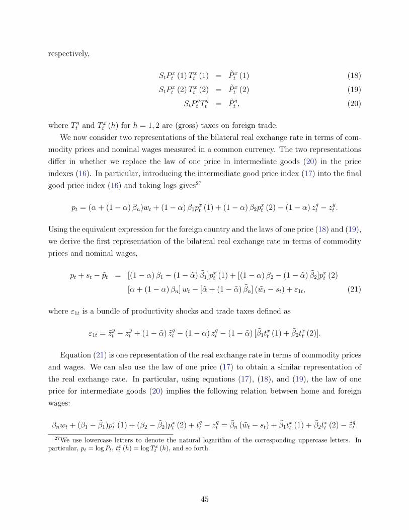
respectively,

StPxt (1)T xt (1) = P x

t (1) (18)

StPxt (2)T xt (2) = P x

t (2) (19)

StPqt T

qt = P q

t , (20)

where T qt and T xt (h) for h = 1, 2 are (gross) taxes on foreign trade.

We now consider two representations of the bilateral real exchange rate in terms of com-

modity prices and nominal wages measured in a common currency. The two representations

differ in whether we replace the law of one price in intermediate goods (20) in the price

indexes (16). In particular, introducing the intermediate good price index (17) into the final

good price index (16) and taking logs gives27

pt = (α + (1− α) βn)wt + (1− α) β1pxt (1) + (1− α) β2p

xt (2)− (1− α) zqt − z

yt .

Using the equivalent expression for the foreign country and the laws of one price (18) and (19),

we derive the first representation of the bilateral real exchange rate in terms of commodity

prices and nominal wages,

pt + st − pt = [(1− α) β1 − (1− α) β1]pxt (1) + [(1− α) β2 − (1− α) β2]p

xt (2)

[α + (1− α) βn]wt − [α + (1− α) βn] (wt − st) + ε1t, (21)

where ε1t is a bundle of productivity shocks and trade taxes defined as

ε1t = zyt − zyt + (1− α) zqt − (1− α) zqt − (1− α) [β1t

xt (1) + β2t

xt (2)].

Equation (21) is one representation of the real exchange rate in terms of commodity prices

and wages. We can also use the law of one price (17) to obtain a similar representation of

the real exchange rate. In particular, using equations (17), (18), and (19), the law of one

price for intermediate goods (20) implies the following relation between home and foreign

wages:

βnwt + (β1 − β1)pxt (1) + (β2 − β2)pxt (2) + tqt − zqt = βn (wt − st) + β1t

xt (1) + β2t

xt (2)− zqt .

27We use lowercase letters to denote the natural logarithm of the corresponding uppercase letters. Inparticular, pt = logPt, t

xt (h) = log T x

t (h), and so forth.

45

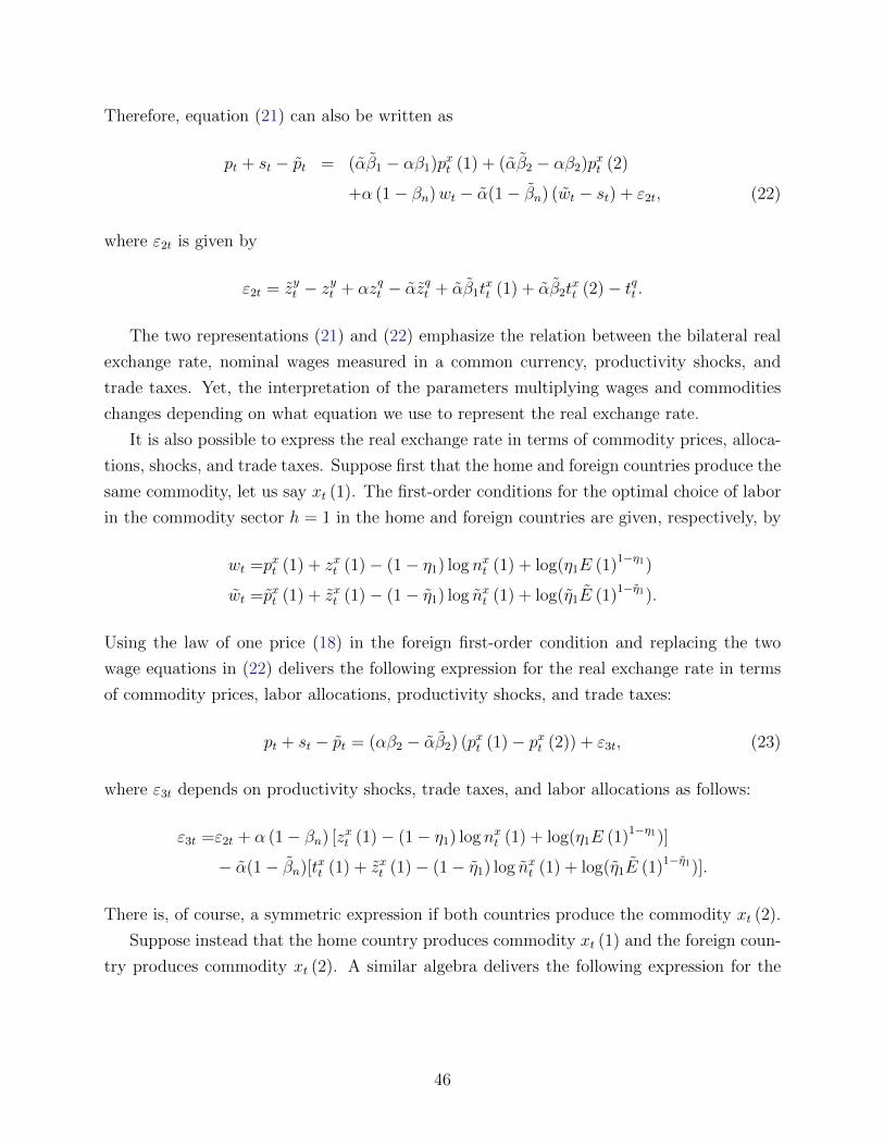
Therefore, equation (21) can also be written as

pt + st − pt = (αβ1 − αβ1)pxt (1) + (αβ2 − αβ2)pxt (2)

+α (1− βn)wt − α(1− βn) (wt − st) + ε2t, (22)

where ε2t is given by

ε2t = zyt − zyt + αzqt − αz

qt + αβ1t

xt (1) + αβ2t

xt (2)− tqt .

The two representations (21) and (22) emphasize the relation between the bilateral real

exchange rate, nominal wages measured in a common currency, productivity shocks, and

trade taxes. Yet, the interpretation of the parameters multiplying wages and commodities

changes depending on what equation we use to represent the real exchange rate.

It is also possible to express the real exchange rate in terms of commodity prices, alloca-

tions, shocks, and trade taxes. Suppose first that the home and foreign countries produce the

same commodity, let us say xt (1). The first-order conditions for the optimal choice of labor

in the commodity sector h = 1 in the home and foreign countries are given, respectively, by

wt =pxt (1) + zxt (1)− (1− η1) log nxt (1) + log(η1E (1)1−η1)

wt =pxt (1) + zxt (1)− (1− η1) log nxt (1) + log(η1E (1)1−η1).

Using the law of one price (18) in the foreign first-order condition and replacing the two

wage equations in (22) delivers the following expression for the real exchange rate in terms

of commodity prices, labor allocations, productivity shocks, and trade taxes:

pt + st − pt = (αβ2 − αβ2) (pxt (1)− pxt (2)) + ε3t, (23)

where ε3t depends on productivity shocks, trade taxes, and labor allocations as follows:

ε3t =ε2t + α (1− βn) [zxt (1)− (1− η1) log nxt (1) + log(η1E (1)1−η1)]

− α(1− βn)[txt (1) + zxt (1)− (1− η1) log nxt (1) + log(η1E (1)1−η1)].

There is, of course, a symmetric expression if both countries produce the commodity xt (2).

Suppose instead that the home country produces commodity xt (1) and the foreign coun-

try produces commodity xt (2). A similar algebra delivers the following expression for the

46

real exchange rate:

pt + st − pt = (αβ1 + α (1− βn − β1)) (pxt (1)− pxt (2)) + ε4t, (24)

where ε4t is now given by

ε4t =ε2t + α (1− βn) [zxt (1)− (1− η1) log nxt (1) + log(η1E (1)1−η1)]

− α(1− βn)[txt (2) + zxt (2)− (1− η2) log nxt (2) + log(η2E (2)1−η2)].

Again, there is a symmetric representation if the home country produces xt (2) and the

foreign country produces xt (1).

In obtaining the real exchange rate representations (23) and (24), we introduced the

labor first-order conditions in the commodities sector into the representation in terms of

wages (22). We could have used instead the cost minimization conditions in the final good’s

sector,Wt

P qt

=α

1− αqtnyt

andWt

P qt

=α

1− αqtnyt, (25)

to replace nominal wages in equation (22). Inserting these expressions into (22) gives a

representation of the real exchange rate in terms of commodity prices, intermediate good

prices measured in a common currency, productivity shocks, trade taxes, and allocations:

pt + st − pt =(αβ1 − αβ1)pxt (1) + (αβ2 − αβ2)pxt (2) (26)

+ α (1− βn) pqt − α(1− βn) (pqt − st) + ε5t,

where

ε5t =ε2t + α (1− βn) log (qt/nyt )− α(1− βn) log (qt/n

yt )

+ log

(α

1− α

)(α (1− βn)− α(1− βn)).

Finally, we show a representation of the real exchange rate that is independent of com-

modity prices. The cost minimization conditions (25), the price index (17), and the law of

one price in commodities allows us to write

wt(1− βn) = β1pxt (1) + β2p

xt (2)− zqt + log

(α

1− αqtnyt

)(wt − st) (1− βn) = β1 [pxt (1) + txt (1)] + β2 [pxt (2) + txt (2)]− zqt + log

(α

1− αqtnyt

).

47

Replacing these expressions in (22) delivers the representation real exchange rate that is

independent of commodity prices,

pt + st − pt = zyt − zyt − t

qt + α log (qt/nt)− α log (qt/nt) + κ, (27)

where κ = α log (α/ (1− α))− α log (α/ (1− α)) is a constant.

48

G General Technologies

In this section we show that the simple case with Cobb-Douglas technologies general-

izes, in an appropriate fashion, to general constant returns to scale production functions.

The equilibrium prices in the final good sector and the intermediate good sector can be

represented by the marginal cost function

Pt = Cy (Wt, Pqt ) /Zy

t (28)

P qt = Cq (Wt, P

xt (1) , P x

t (2)) /Zqt (29)

Replacing (28) with (29) and using that the cost function is homogeneous of degree one in

factor prices, we can write the price of the final good as

Pt = P xt (1) c

(Wt

P xt (1)

,P xt (2)

P xt (1)

)/Zy

t

with a similar expression for the foreign country,

Pt = P xt (1) c

(Wt

P xt (1)

,P xt (2)

P xt (1)

)/Zy

t .

The real exchange rate is then defined as

rert =c(

Wt

Pxt (1)

,Pxt (2)

Pxt (1)

)c(

Wt

Pxt (1)

,Pxt (2)

Pxt (1)

) Zyt

Zyt

P xt (1)St

P xt (1)

.

Using the law of one price for the commodities,

rert =c(

Wt

Pxt (1)

,Pxt (2)

Pxt (1)

)c(

Wt

Pxt (1)

,Pxt (2)

Pxt (1)

Txt (2)

Txt (1)

) Zyt /Z

yt

T xt (1). (30)

Let the technology to produce commodity i = 1, 2 be given by Xt (i) = Zxt (i)Fi (n

xt (i)).

The first-order condition with respect to labor is then given by

Wt/Pxt (i) = Zx

t (i)F ′ (nxt (i)) .

Suppose that both countries produce commodity Xt (1). Then replacing the previous con-

dition evaluated at i = 1 in (30) gives the first representation of the real exchange rate in

49

terms of commodity prices and labor allocations,

rert =c(Zxt (1)F ′1 (nxt (1)) ,

Pxt (2)

Pxt (1)

)c(Zxt (1)F ′1 (nxt (1)) ,

Pxt (2)

Pxt (1)

Txt (2)

Txt (1)

) Zyt /Z

yt

T xt (1). (31)

Suppose instead that the home country produces commodity X (1) but the foreign country

produces commodity X (2). The real exchange rate can then be written as

rert =c(Zxt (1)F ′1 (nxt (1)) ,

Pxt (2)

Pxt (1)

)c(Zxt (2)F ′2 (nxt (2))

Pxt (2)

Pxt (1)

,Pxt (2)

Pxt (1)

) Zyt /Z

yt

T xt (2), (32)

which is our second representation of the real exchange rate.

To obtain our third representation of the real exchange rate, we use the cost minimization

condition in the final goods’ sector, which can be written as

Wt

P qt

= h

(nytqt

)(33)

where h is a decreasing function. Using this expression in (30) delivers

rert =c(h(nyt

qt

)P qt

Pxt (1)

,Pxt (2)

Pxt (1)

)c(h(nyt

qt

)P qt

Pxt (1)

,Txt (2)

Txt (1)

) Zyt /Z

yt

T xt (1). (34)

This expression relates the real exchange rate to relative commodity prices, to the relative

price of the intermediate good in terms of commodity X (1), and to the allocation.

Finally, we obtain an expression independent of commodity prices. To that end, we use

that the equilibrium price in the intermediate goods’ sector (29) can be written as

P qt

P xt (1)

= φ

(Wt

P xt (1)

,P xt (2)

P xt (1)

)/Zq

t .

But (33) impliesWt

P xt (1)

=P qt

P xt (1)

h

(nytqt

),

which, using the previous expression, becomes

Wt

P xt (1)

= φ

(Wt

P xt (1)

,P xt (2)

P xt (1)

)h

(nytqt

)/Zq

t .

50

Using the properties of the cost function,

1 = φ

(1,P xt (2) /P x

t (1)

Wt/P xt (1)

)h

(nytqt

)1

Zqt

.

This is an implicit function which delivers

Wt

P xt (1)

=P xt (2)

P xt (1)

κ

(nytqt, Zq

t

).

The equivalent expression for the foreign country (using the law of one price for the com-

modities) isWt

P xt (1)

=P xt (2)

P xt (1)

T xt (2)

T xt (1)κ

(nytqt, Zq

t

).

Using the latter two expressions in (30) gives the last representation of the real exchange

rate,

rert =c(Pxt (2)

Pxt (1)

κ(nyt

qt, Zq

t

),Pxt (2)

Pxt (1)

)c(Pxt (2)

Pxt (1)

Txt (2)

Txt (1)

κ(nyt

qt, Zq

t

),Pxt (2)

Pxt (1)

Txt (2)

Txt (1)

) Zyt /Z

yt

T xt (1).

The properties of the cost function imply that the relative prices P xt (2) /P x

t (1) disappear,

rert =c(κ(nyt

qt, Zq

t

), 1)

c(Txt (2)

Txt (1)

κ(nyt

qt, Zq

t

),Txt (2)

Txt (1)

) Zyt /Z

yt

T xt (1). (35)

51

H Multiple Consumption Goods

In this section we assume that there are many different types of (nontraded) consumption

goods. In particular, we assume that there are k = 1, ..., K types of consumption goods.

Households in each country value the basket of consumption goods

K∏k=1

Ct(k)ρ(k),

in which the coefficients, ρ(k), add up to one. Again, we allow for different coefficients, ρ(k),

across countries. Each consumption good is produced according to the technology

Ct(k) = ZCt (k)

(J∏j=1

[nC(k)t (j)]ψ

C(k,j)

)α( N∏i=1

qC(k)t (i)ϕ(k,i)

)1−α

.

The rest of the economy (the production of intermediate goods and commodities) has

the same structure as in Section 5.

H.1 Prices

Let Pt denote the price of the basket of goods and PCt (k) the price of the type-k con-

sumption good. Households’ cost-minimization problem over different types of consumption

goods implies that, in equilibrium, the price of the basket satisfies

lnPt =K∑k=1

ρ(k) lnPCt (k).

Next, we use the fact that the price of each type of consumption good will be Cobb-

Douglas functions of factor prices (see Section 5.1). So we reach the equivalent of equation

(6) for the case of multiple consumption goods:

lnPt =K∑k=1

ρ(k)

ln(κC(k)

ZCt (k)

)+ α

∑Jj=1 ψ

C (k, j) lnWt (j) +

(1− α)∑N

i=1 ϕ (k, i) lnPQt (i)

,which is now a sum over the different types of consumption goods. Therefore, we can follow

the same steps as described in Section 5.1 in order to derive a relationship between bilateral

real exchange rates and PCP that resembles equation (15). The only difference in the case

of multiple consumption goods is that the relationship between PCP and real exchange rates

52

will also depend on the difference in preferences over the types of consumption goods across

countries, that is, differences in the coefficients ρ(k).

53

I Sum of coefficients

In this appendix, we show that the sum of the coefficients in prices and wages in expression

(8), repeated here for convenience,

lnPt = lnκC

zyt+ (1− α)

N∑i=1

ϕ (i)κQ(i)

zt(i)

+J∑j=1

[αψC (j) +

N∑i=1

(1− α)ϕ (i) β(i)ψQ (i, j)

]lnWt (j)

+ (1− α)N∑i=1

ϕ (i) (1− β(i))N∑h=1

γ(i, h) lnPt(h),

add up to 1. The sum of the coefficients is

J∑j=1

[αψC(j) + (1− α)N∑i=1

β(i)ϕ(i)ψQ(i, j)] + (1− α)N∑h=1

N∑i=1

(1− β(i))ϕ(i)γ(i, h),

which can be written

αJ∑j=1

ψC(j) + (1− α)N∑i=1

β(i)ϕ(i)J∑j=1

ψQ(i, j) + (1− α)N∑i=1

(1− β(i))ϕ(i)N∑h=1

γ(i, h)

or

α + (1− α)N∑i=1

β(i)ϕ(i) + (1− α)N∑i=1

(1− β(i))ϕ(i)

= α + (1− α)N∑i=1

β(i)ϕ(i) + (1− α)− (1− α)N∑i=1

β(i)ϕ(i) = 1.

54

Documents

Real Exchange Rates and Primary Commodity Prices Exchange Rates and Primary Commodity ... Real Exchange Rates and Primary Commodity Prices ... against the US dollar can be accounted