Embed Size (px)
DESCRIPTION
Real Estate Space and Asset Markets. Module 1: Real Estate Investment Analysis. Two Types of Real Estate Markets. A market is a mechanism for the voluntary exchange of goods and services among owners. - PowerPoint PPT Presentation
Citation preview
Real Estate Space and Asset Markets
Module 1:Real Estate Investment Analysis

2
Two Types of Real Estate Markets
A market is a mechanism for the voluntary exchange of goods and services among owners.
There are two types of real estate markets for our consideration in this course. They are:Real Estate Space MarketReal Estate Asset Market
3
Real Estate Space Market
The term “space market” is the market for the usage of real property.
In this market, tenants exchange rent with landlords for the right to use land and built space.
This market is often called “the rental market.”
4
Real Estate Asset Market
The term “asset market” refers to the mechanism for the voluntary exchange of ownership of real property.
In this market, buyers exchange money with sellers for ownership rights to land and built space (real estate).
This market is often called “the property market.”
5
Let’s first consider several characteristics of “space markets.” After that, we will look at the characteristics of “asset markets.”
6
Characteristics of the Space Market: Demand and Supply
Demand side of this type of market includes individuals, households, or firms who want to use space for consumption or production purposes.
Supply side of this type of market includes real estate owners who “rent” (used as a verb here) space to tenants.
7
Characteristics of the Space Market: Rent
“Rent” as noun refers to the price of the right to use space for a period of time.
May be measured in $ per square foot per year (office space), $ per month per unit (apartments) or various other methods.
Determined by the interaction of supply and demand forces.
8
Characteristics of the Space Market: Equilibrium
When the quantity of space demanded equals the quantity supplied, the market is in equilibrium.
The observed rent at equilibrium is called market rent.
9
Characteristics of the Space Market: Market Rent Changes
The principle of supply and demand states that equilibrium price in a market is directly related to changes in demand and inversely related to changes in supply.
Market rent, therefore, is directly related to changes in demand and inversely related to changes in supply.
10
Characteristics of the Space Market: Segmentation
The real estate space market is highly segmented, meaning that it tends to be local in nature and specialized by property usage.
Within each segment, or submarket, the same good may have a different equilibrium price.
Market rent for office space may differ significantly between Seattle and Miami.
Market rent for retail space and warehouse space in the same city may different dramatically.
11
Why is the Real Estate Space Market Segmented?
On the demand side:Users require specific types of spaceUsers require specific locations
On the supply side:Buildings are built for specific usesBuildings are fixed in location
Thus, we often talk of “geographic” or “property usage” submarkets.
12
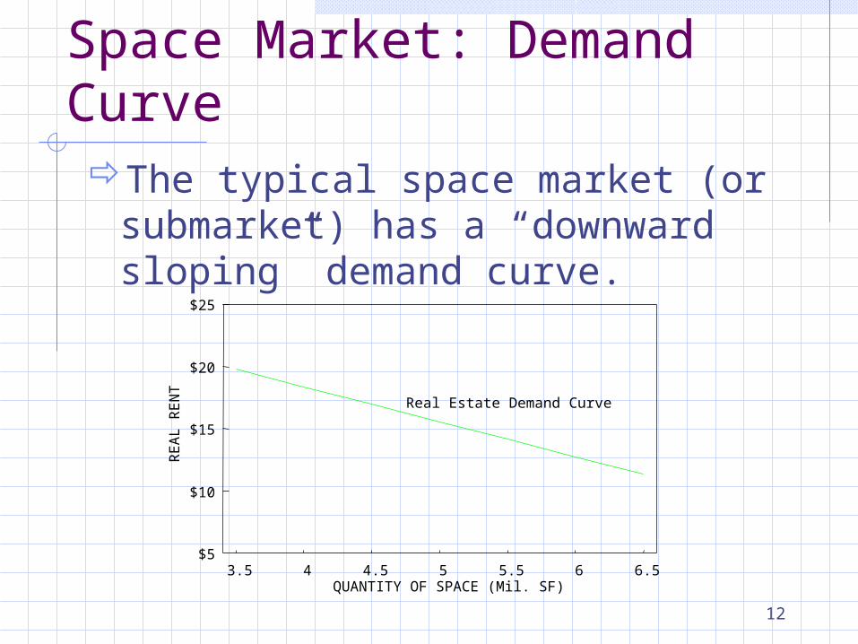
Characteristics of the Space Market: Demand CurveThe typical space market (or
submarket) has a “downward sloping” demand curve.
$5
$10
$15
$20
$25
QUANTITY OF SPACE (Mil. SF)
RE
AL
RE
NT
3.5 4 4.5 5 5.5 6 6.5
Real Estate Demand Curve
13
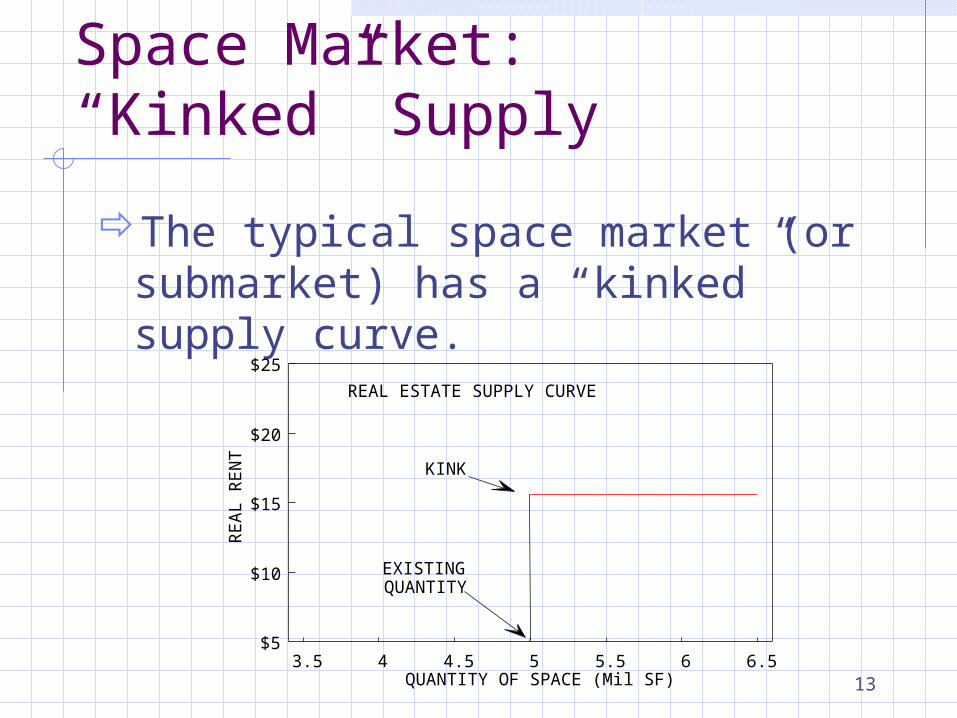
Characteristics of the Space Market: “Kinked” Supply
The typical space market (or submarket) has a “kinked” supply curve.
$5
$10
$15
$20
$25
QUANTITY OF SPACE (Mil SF)
RE
AL
RE
NT
3.5 4 4.5 5 5.5 6 6.5
KINK
REAL ESTATE SUPPLY CURVE
EXISTINGQUANTITY
14
Characteristics of the Space Market: Why these shapes?
The shape of the demand curve makes sense when we consider that users will prefer more space when prices are low than they will when prices are high.
The shape of the supply curve (kinked) makes sense when we consider that the amount of built space is fixed in the short run because it takes a long time to add new space and because existing space lasts a long time.

15
Characteristics of the Space Market: Where is the Kink?
The kink occurs at the price equal to the marginal cost of adding new space to the submarket.
From basic economics, we know that the supply function for a competitively produced product equals the marginal cost function.
The marginal cost of built space includes site acquisition costs, construction costs, and the developer’s necessary profits.
16
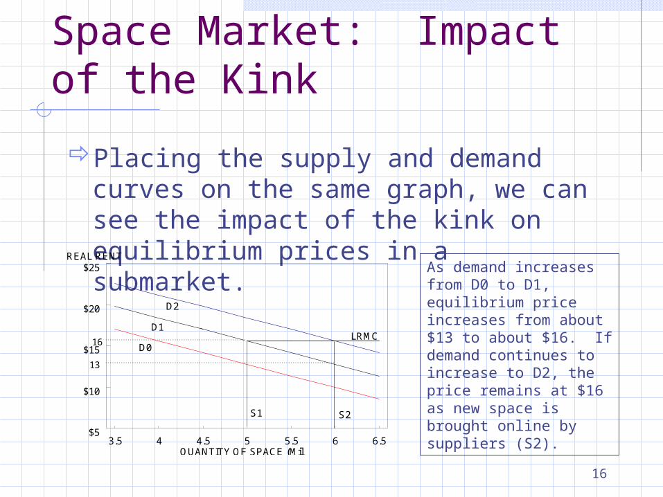
Characteristics of the Space Market: Impact of the Kink
Placing the supply and demand curves on the same graph, we can see the impact of the kink on equilibrium prices in a submarket.
$5
$10
$15
$20
$25
QUANTITY OF SPACE (Mil
REAL RENT
3.5 4 4.5 5 5.5 6 6.5
D0
D1
D2
S1 S2
LRMC16
13
As demand increases from D0 to D1, equilibrium price increases from about $13 to about $16. If demand continues to increase to D2, the price remains at $16 as new space is brought online by suppliers (S2).
17
Some Important Observations
In submarkets with rising long-run marginal costs (rising land prices make the next building more expensive than the prior one), the supply curve is increasing beyond the existing supply quantity.
In submarkets with falling long-run marginal costs (the next building is cheaper to construct than the prior one), the supply curve is decreasing beyond the existing supply quantity.
In most U.S. space submarkets, the supply curve is flat beyond the existing supply quantity because the next building probably costs the same as the previous one (in real terms).
18
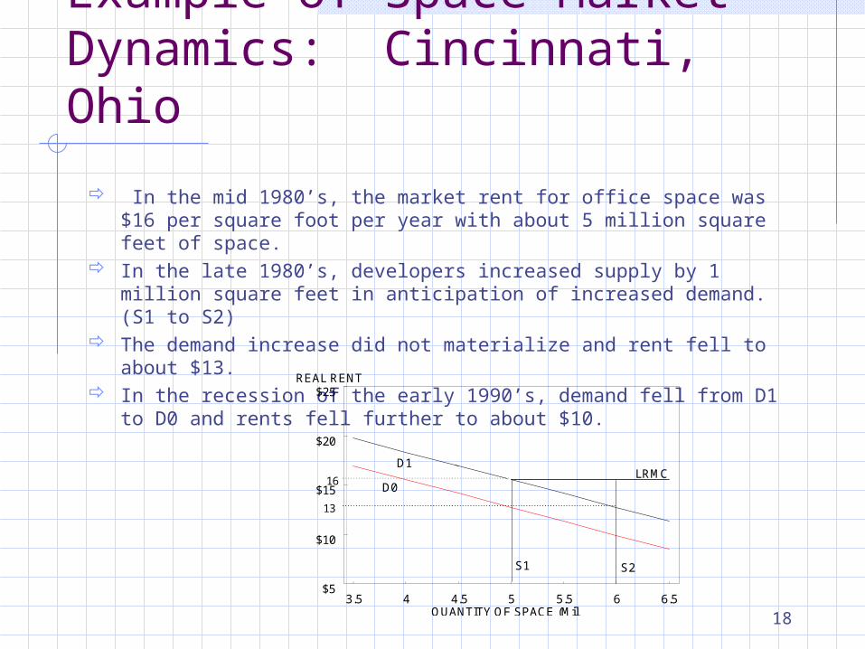
Example of Space Market Dynamics: Cincinnati, Ohio
In the mid 1980’s, the market rent for office space was $16 per square foot per year with about 5 million square feet of space.
In the late 1980’s, developers increased supply by 1 million square feet in anticipation of increased demand. (S1 to S2)
The demand increase did not materialize and rent fell to about $13. In the recession of the early 1990’s, demand fell from D1 to D0 and
rents fell further to about $10.
$5
$10
$15
$20
$25
QUANTITY OF SPACE (Mil
REAL RENT
3.5 4 4.5 5 5.5 6 6.5
D0
D1
S1 S2
LRMC 16
13
19
Characteristics of the Asset Market:
“Asset market” refers to the market for the ownership of real estate assets (land and the buildings on it) rather than the use of space in real estate assets.
Buyers in this market purchase real estate in expectation of receiving future cash flows (rent paid by tenants).
These buyers could buy other kinds of assets (stocks, bonds, etc.) that would also produce future earnings.
In this sense, the real estate asset market is really a part of the larger capital market.
20
Overview of Capital Markets
Capital markets can be divided into four categoriesPublic equity marketsPrivate equity marketsPublic debt marketsPrivate equity markets
Where do real estate assets fit? In all four categories, in some
fashion!
21
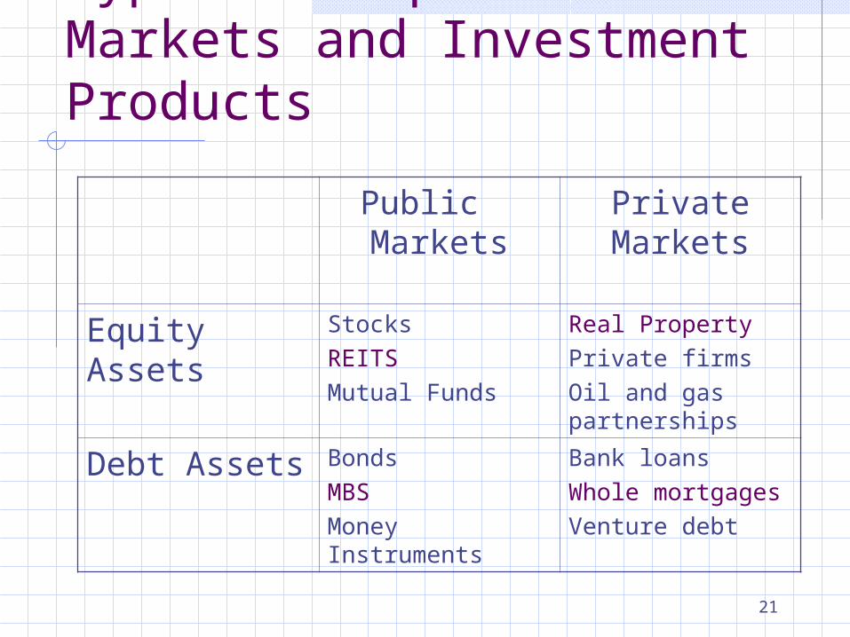
Types of Capital Asset Markets and Investment Products
Public Markets
Private Markets
Equity Assets StocksREITSMutual Funds
Real PropertyPrivate firmsOil and gas partnerships
Debt Assets BondsMBSMoney Instruments
Bank loansWhole mortgagesVenture debt
22
Characteristics of Capital Markets
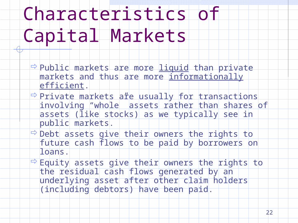
Public markets are more liquid than private markets and thus are more informationally efficient.
Private markets are usually for transactions involving “whole” assets rather than shares of assets (like stocks) as we typically see in public markets.
Debt assets give their owners the rights to future cash flows to be paid by borrowers on loans.
Equity assets give their owners the rights to the residual cash flows generated by an underlying asset after other claim holders (including debtors) have been paid.
23
Pricing Real Estate Assets
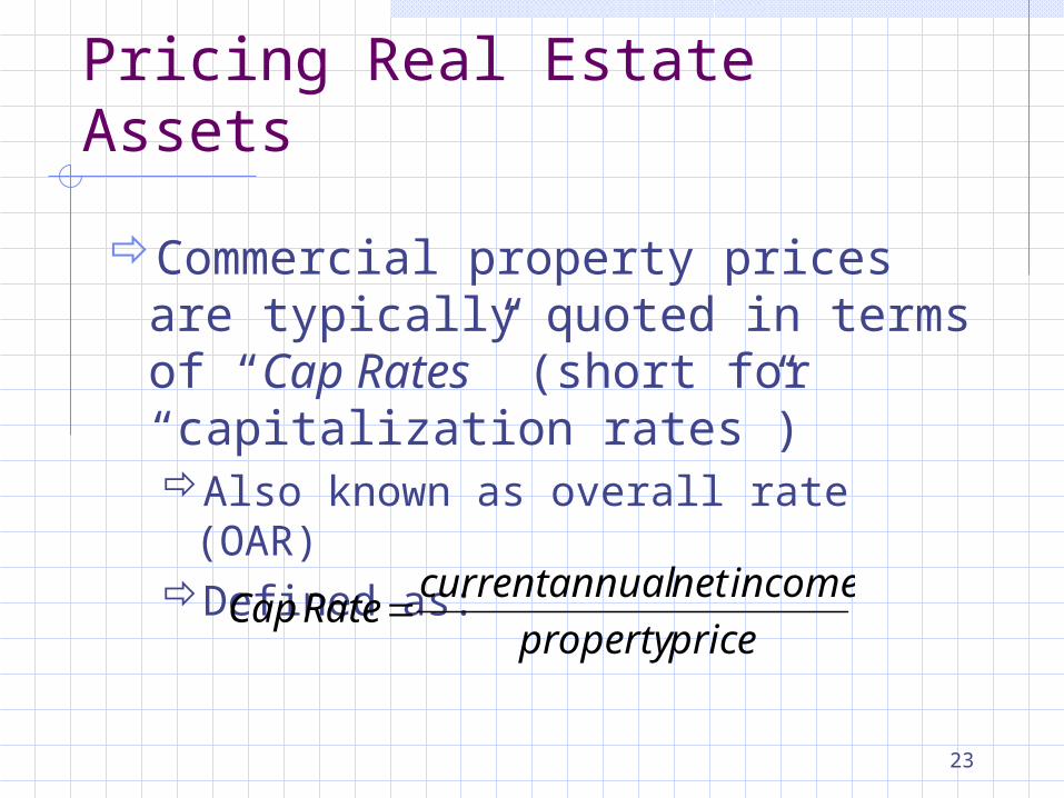
Commercial property prices are typically quoted in terms of “Cap Rates” (short for “capitalization rates”) Also known as overall rate (OAR)Defined as:
priceproperty
incomenetannualcurrentRateCap
24
Characteristics of Cap Rates
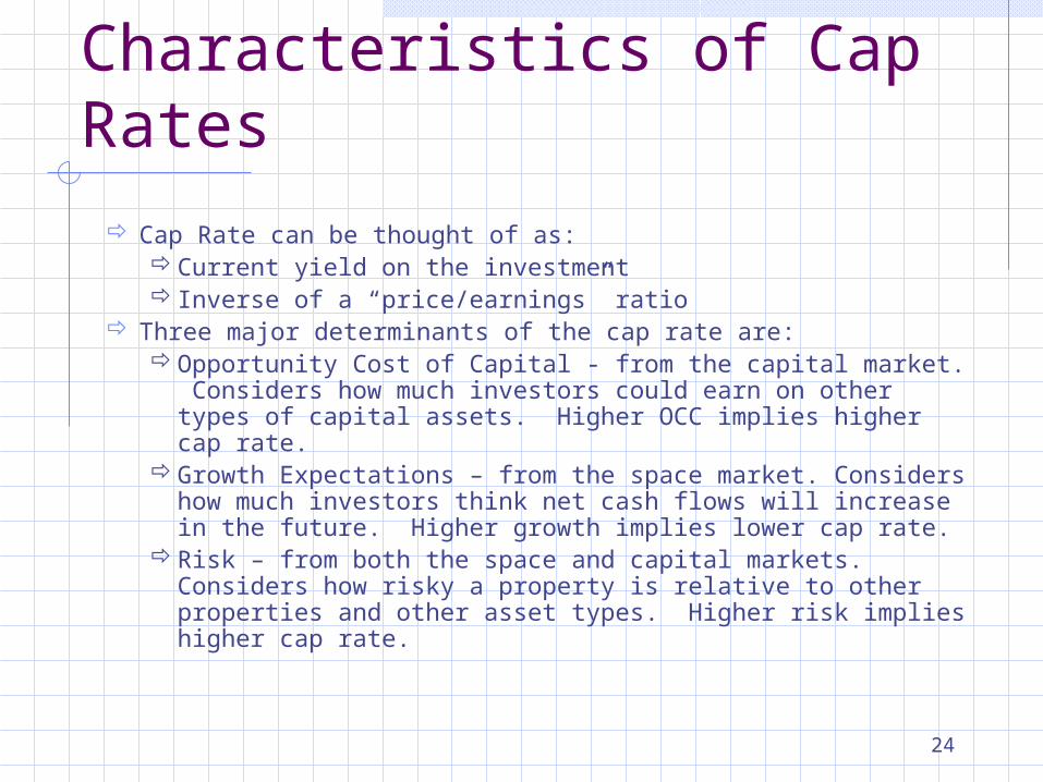
Cap Rate can be thought of as:Current yield on the investment Inverse of a “price/earnings” ratio
Three major determinants of the cap rate are:Opportunity Cost of Capital - from the capital market.
Considers how much investors could earn on other types of capital assets. Higher OCC implies higher cap rate.
Growth Expectations – from the space market. Considers how much investors think net cash flows will increase in the future. Higher growth implies lower cap rate.
Risk – from both the space and capital markets. Considers how risky a property is relative to other properties and other asset types. Higher risk implies higher cap rate.
25
Is the Asset Market Segmented? No (not very)
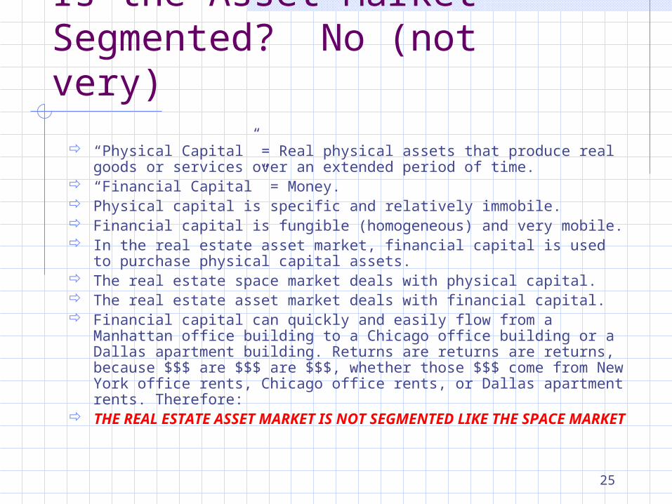
“Physical Capital” = Real physical assets that produce real goods or services over an extended period of time.
“Financial Capital” = Money. Physical capital is specific and relatively immobile. Financial capital is fungible (homogeneous) and very mobile. In the real estate asset market, financial capital is used to purchase physical
capital assets. The real estate space market deals with physical capital. The real estate asset market deals with financial capital. Financial capital can quickly and easily flow from a Manhattan office building to
a Chicago office building or a Dallas apartment building. Returns are returns are returns, because $$$ are $$$ are $$$, whether those $$$ come from New York office rents, Chicago office rents, or Dallas apartment rents. Therefore: THE REAL ESTATE ASSET MARKET IS NOT SEGMENTED LIKE THE
SPACE MARKET
26
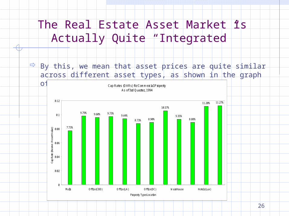
The Real Estate Asset Market is Actually Quite “Integrated”
By this, we mean that asset prices are quite similar across different asset types, as shown in the graph of cap rates.
Cap Rates (OARs) for Commercial PropertyAs of 3rd Quarter, 1994
7.73%
9.79% 9.60% 9.73%9.44%
8.73% 8.90%
10.57%
9.35%8.88%
11.20% 11.27%
0
0.02
0.04
0.06
0.08
0.1
0.12
Malls Office(CBD) Office(LA) Office(DC) Warehouse Hotels(Lux)
Property Type/Location
Cap
Rate
(Inc
ome
/ Ass
et V
alue
)
27
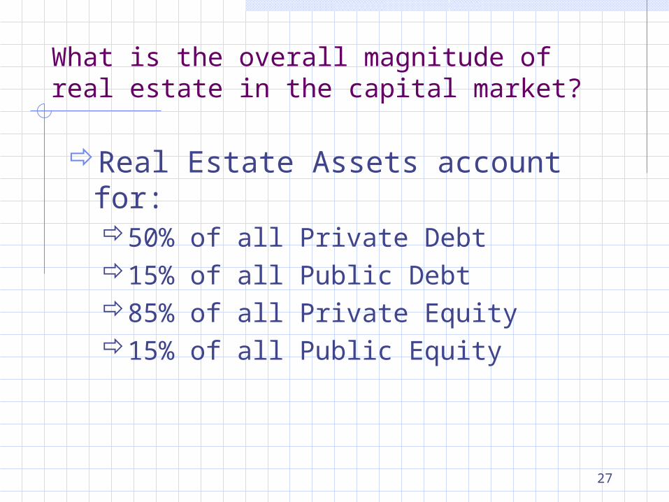
What is the overall magnitude of real estate in the capital market?
Real Estate Assets account for:50% of all Private Debt15% of all Public Debt85% of all Private Equity15% of all Public Equity
28
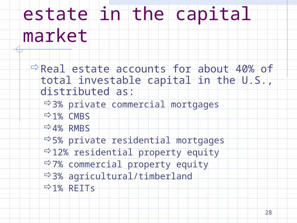
Another view of real estate in the capital market
Real estate accounts for about 40% of total investable capital in the U.S., distributed as:3% private commercial mortgages1% CMBS4% RMBS5% private residential mortgages12% residential property equity7% commercial property equity3% agricultural/timberland1% REITs
The Real Estate System
Module 3:Real Estate Investment Analysis

30
What Links the Asset and Space Markets?
The real asset and space markets discussed in the previous module are linked together by the development industry.
The manner in which the development industry accomplishes this complex task is the focus of this module.
The development industry, the real estate asset market, and the real estate space market together form the real estate system.

31
Property Development Industry
Property development is a creative, entrepreneurial process characterized by…VisionGreedCooperationRisk
(Some of the most entertaining features of American capitalism.)
32
Development is highly cyclical.
Buildings are “long-lived” assets, it is only the demand for new built space that supports the development industry.
Because this demand is sensitive to general economic changes, the development industry is subject to “boom-bust” cycles.
33
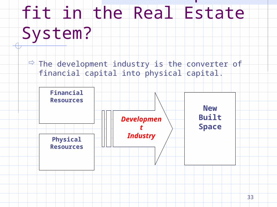
Where does Development fit in the Real Estate System?
The development industry is the converter of financial capital into physical capital.
FinancialResources
PhysicalResources
NewBuilt
SpaceDevelopmentIndustry
34
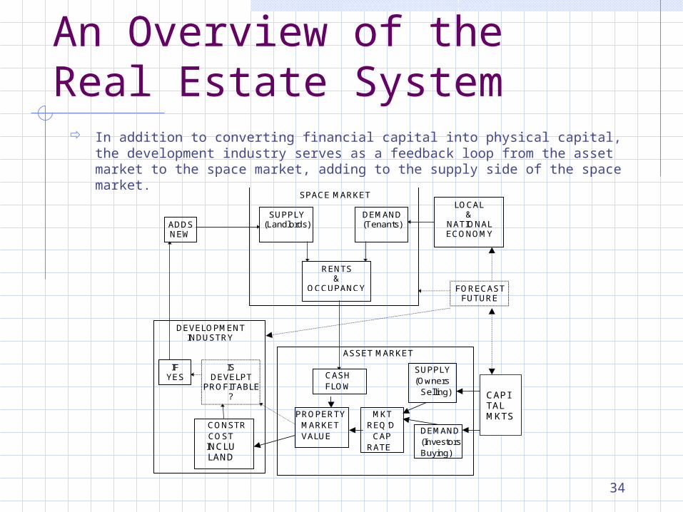
An Overview of the Real Estate System
In addition to converting financial capital into physical capital, the development industry serves as a feedback loop from the asset market to the space market, adding to the supply side of the space market.
SPACE MARKET
SUPPLY (Landlords)
DEMAND (Tenants)
RENTS &
OCCUPANCY
LOCAL &
NATIONAL ECONOMY
FORECAST FUTURE
ASSET MARKET
SUPPLY
(Owners
Selling)
DEMAND
(Investors
Buying)
CASH
FLOW
MKT
REQ’D
CAP
RATE
PROPERTY
MARKET
VALUE
DEVELOPMENT INDUSTRY
IS DEVELPT
PROFITABLE ?
CONSTR
COST INCLU LAND
IF YES
ADDS NEW
CAPITAL MKTS
35
The 4-Quadrant Model
To explain the long-run equilibrium simultaneously between and within the asset and space markets requires a more detailed model than the simple supply/demand model.
We will consider the DisPasquale-Wheaton “4-Quadrant Model” that depicts four distinct relationships simultaneously.
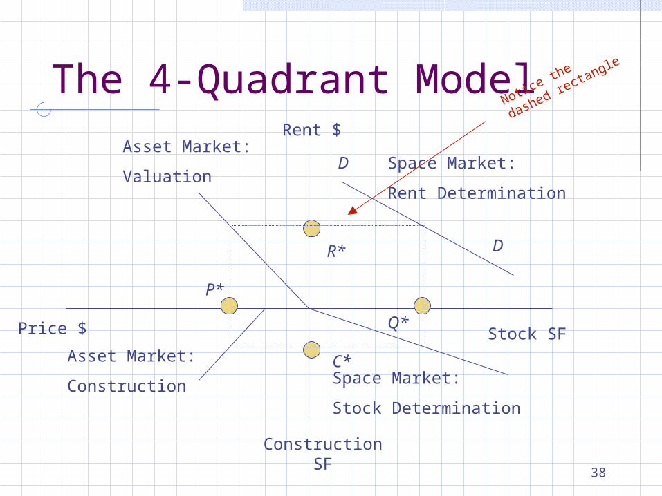
The model is really nothing more than 4 simple graphs shown with a dashed rectangle linking them together.

36
A Personal Note:
My eyes glazed over and I started sweating profusely the first time I looked at this model and heard one of its authors discuss it at an academic conference, but it’s really not so bad when you understand its component parts.
Once I took it apart and put it back together, I discovered it is a pretty clever way to describe about how things “work” in real estate markets.
Our text book authors do a great job of explaining the model, but it may take several “readings” before you fully grasp it.
37
The 4-Q’s in the 4-Quadrant Model
The four main issues addressed by the model are:How are rents determined in the space
market? (NE quadrant)How are properties valued in the asset
market? (NW quadrant)What determines the amount of new
construction? (SW quadrant)How is new construction related to the
existing stock of space? (SE quadrant)
38
The 4-Quadrant ModelRent $
Space Market:
Rent Determination
Space Market:
Stock Determination
Asset Market:
Construction
Asset Market:
Valuation
Stock SF
Construction SF
Price $
P*
R*
Q*
C*
D
D
Notice the dashed
rectangle
39
Northeast Quadrant: Rent Determination
Horizontal axis is the physical stock of space in the market in square feet.
Vertical axis is the rent for space in $ per square foot per year.
Demand for space is shown as the downward sloping line, just as in the familiar supply/demand model.
Existing space is shown as Q*Equilibrium rent is shown as R*
40
Northwest Quadrant: Valuation
Horizontal axis is price per square foot of space in the asset market.
Vertical axis is the rent per square foot of space.
The line represents the cap rate, which we know expresses the price of real estate as a yield measure.
The equilibrium price is shown as P* Note the we are assuming that prices increase as we
move left along the horizontal axis in this quadrant.
41
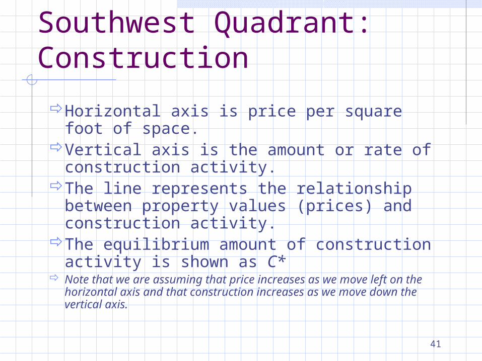
Southwest Quadrant: Construction
Horizontal axis is price per square foot of space.
Vertical axis is the amount or rate of construction activity.
The line represents the relationship between property values (prices) and construction activity.
The equilibrium amount of construction activity is shown as C*
Note that we are assuming that price increases as we move left on the horizontal axis and that construction increases as we move down the vertical axis.
42
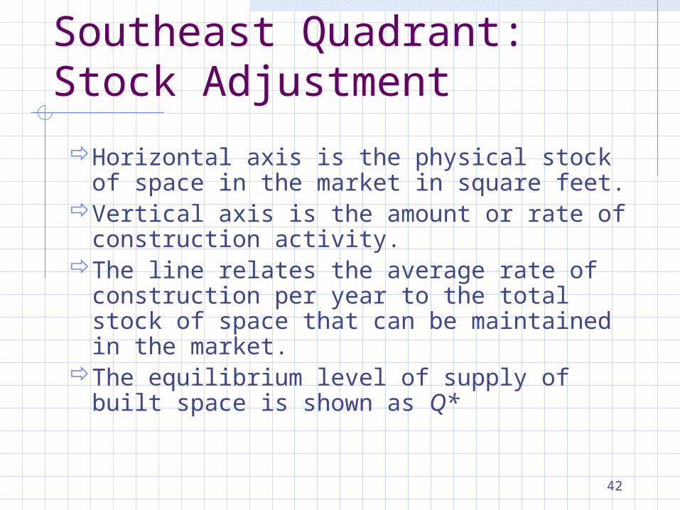
Southeast Quadrant: Stock Adjustment
Horizontal axis is the physical stock of space in the market in square feet.
Vertical axis is the amount or rate of construction activity.
The line relates the average rate of construction per year to the total stock of space that can be maintained in the market.
The equilibrium level of supply of built space is shown as Q*
43
What’s the Big Deal about the 4Q Model?
The 4-Quadrant model helps explain Boom and Bust Cycles in Real Estate Markets.
Boom means that space markets see an extended rise in occupancy and rents.
Bust means that space markets see an extended period of falling occupancy and rents.
Similarly, property prices (in the asset market) tend to exhibit periods of rising and falling prices corresponding to ups and downs in the space market.
44
Demand increases can trigger a boom-bust cycle
Let’s use the model to see how an increase in demand can lead to a boom-bust cycle.
To do so, we first must understand how the model responds to two types of demand changesDemand changes in the space
marketDemand changes in the asset market
45
Demand Increase in Space Market
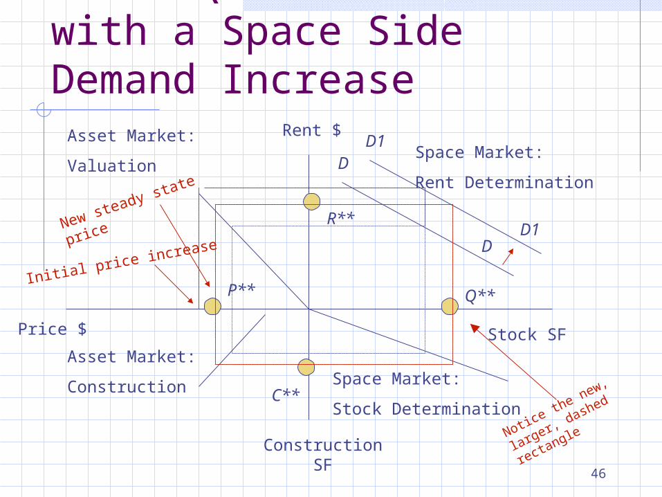
Let the line DD shift to DD1 resulting in a new equilibrium quantity, Q**
The initial reaction is a dramatic price increase (boom).
To maintain a steady state (long run equilibrium), price and other equilibrium points must change as shown by the new, larger dashed rectangle on the next slide.
46
Rent $Space Market:
Rent Determination
Space Market:
Stock Determination
Asset Market:
Construction
Asset Market:
Valuation
Stock SF
Construction SF
Price $
R**
Q**
C**
D
D
Notice the new,
larger, dashed
rectangle
D1
D1
P**
The 4-Quadrant Model with a Space Side Demand Increase
Initial price increase
New steady state
price
47
So, what does the model say?
Initially, a demand increase in the space market would result in a price increase in the asset market, then fall back a bit (bust) as the market returns to its long-run steady state due to new construction.
A demand increase in the space market in the long run results in a rent increasea price increase in the property marketan increase construction an increase equilibrium stock of space
48
Demand Increase in the Asset Market
Continuing along our path to explaining booms and bust, now we will consider what the model tells us about an increase in demand in the asset or property market.
Such an increase is equivalent to an increase in the price investors are willing to pay for real estate per dollar of rental income, or, equivalently, a decrease in the cap rate.
This situation is shown graphically on the next slide.
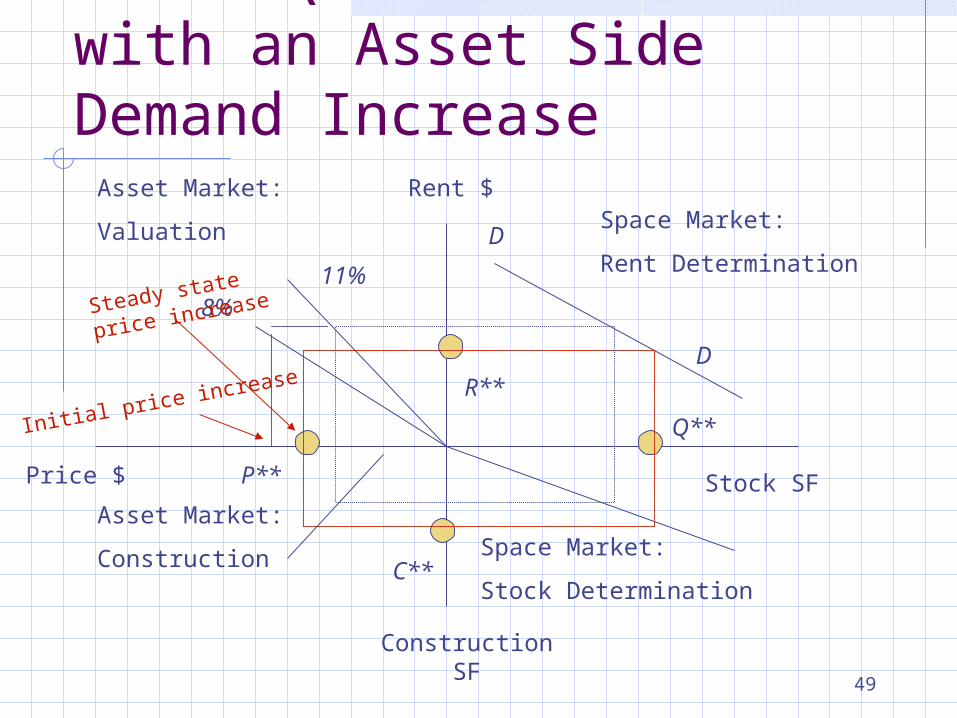
49
Rent $Space Market:
Rent Determination
Space Market:
Stock Determination
Asset Market:
Construction
Asset Market:
Valuation
Stock SF
Construction SF
Price $
R**
Q**
C**
D
D
P**
The 4-Quadrant Model with an Asset Side Demand Increase
11%8%
Initial price increase
Steady state
price increase
50
Now what does the model say?
Initially, prices would rise dramatically (boom), but then fall back a bit (bust) as the market returns to its long-run steady state due to new construction.
An increase in demand in the asset market (lower cap rate) in the long run leads toAn increase in pricesAn increase in construction An increase in equilibrium stock of spaceA decrease in equilibrium rent
51
Back to the Boom-Bust Idea…
We just saw how usage demand growth and investor demand growth can individually cause an “overshooting” of real estate asset pricing.
When both types of demand increases happen simultaneously, the overshooting may be even more dramatic: prices rise significantly, then fall back even deeper, thus exacerbating the boom-bust cycle.
If market participants had perfect foresight about how much prices/rents should initially move, the overshooting would not happen and the cycle would be avoided.
Real Estate Investment Analysis
Module 4: Real Estate Market Analysis
53
Real Estate Market Analysis: Why do it?
The term “real estate market analysis” refers to use of a practical collection of analytical tools and procedures that relate the fundamental principles of real estate market dynamics to the specific decision at hand. Where to locate a branch office? What size or type of building to develop on a specific site? What type of tenants to look for in marketing a particular
building? What the rent and expiration term should be on a given lease? When to begin construction on a development project? How many units to build this year? Which cities and property types to invest in so as to allocate
capital where rents are more likely to grow? Where to locate new retail outlets and/or which stores should
be closed?

54
Broadly Speaking…
Real estate market analysis usually requires quantitative or qualitative understanding (& prediction) of both the demand side and supply side of the space usage market relevant to some real estate decision.The focus might be microlevel, such as a
feasibility analysis for a specific site or propertyOr, the focus might be more general, such as a
general characterization of the supply/demand conditions in a particular space submarket.
55
Variables of Interest in Market Analysis
To evaluate a real estate space submarket, analysts tend to focus on a few primary indicators that characterize both the supply and demand sides of the submarket and the balance (equilibrium) between them.Vacancy rateMarket RentQuantity of new construction startsQuantity of new construction completionsAbsorption of new space
56
Vacancy Rate
By definition, the vacancy rate refers to the percentage of the stock of space in the market that is not currently occupied.Vacancy Rate = Vacant Space/Total SpaceThe vacancy rate reflects the balance between
supply and demand.In most markets, it is normal for some vacancy to
exist (the natural vacancy rate) even when supply and demand are in balance.When actual vacancy rises above the natural vacancy
rate, rents tend to fall.When actual vacancy falls below the natural vacancy rate,
rents tend to increase.
57
Market Rent
By definition, market rent is the level of rents being charged on typical new leases currently being signed in the market.asking rents may differ from effective rentsMarket rent is another indicator of the balance
between supply and demand in a market.Can be tricky to measure because
it is private information andlease terms may differ dramatically from tenant to
tenant
58
Constructions Starts and Completions
Construction is an important “supply side” indicator.“Starts” indicate the amount of space
currently in the “pipeline” and likely to be added to the supply in the near future
“Completes” indicate the amount of space just arriving in the market.
Of course, we need to consider the net addition to supply (after taking demolition and renovations into account).
59
Absorption of New Space
By definition, absorption refers to the amount of additional space that becomes occupied during a year.
Absorption is a “demand side” indicator.Gross absorption – total amount of space
leased, regardless of where tenants come from
Net absorption – net change in the amount of space occupied in a market.
60
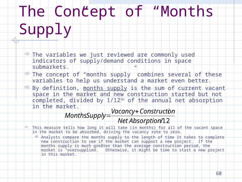
The Concept of “Months Supply”
The variables we just reviewed are commonly used indicators of supply/demand conditions in space submarkets.
The concept of “months supply” combines several of these variables to help us understand a market even better.
By definition, months supply is the sum of current vacant space in the market and new construction started but not completed, divided by 1/12th of the annual net absorption in the market.
This measure tells how long it will take (in months) for all of the vacant space in the market to be absorbed, driving the vacancy rate to zero. Analysts compare the months supply to the length of time it takes to complete
new construction to see if the market can support a new project. If the months supply is much greater than the average construction period, the market is “oversupplied.” Otherwise, it might be time to start a new project in this market.
12/AbsorptionNet
onConstructiVacancySupplyMonths
61
Some Tips for Market Analysis
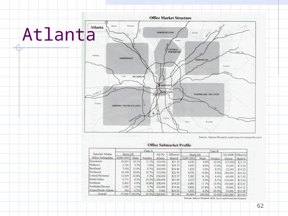
Define the market carefully along geographic and usage dimensions, recognizing that most metropolitan areas form markets that can be usefully divided into smaller submarkets. The next slide describes how the Atlanta office market can be “divided.”
Carefully consider the time period to be covered in the analysis 5 – 10 years into the future is desirable 3 years is more feasible in most cases
Recognize the differences between and the benefits of a simple trend extrapolation and a structural analysis Trend extrapolation predicts the future purely based on
historical trends and patterns Structural analysis attempts to predict the future by identifying
and quantifying the underlying determinants of market trends.
62
Atlanta
63
Performing a Market Analysis
In both types of analysis (extrapolation and structural) the steps are: First, inventory the existing supply and evaluate the pipeline. Second, relate the demand sources to the space usage
demand. Third, forecast future demand for and supply of space Compare the forecasted demand for space with the
forecasted supply of space to see if the market will be “over” or “under” supplied in the future.
In tight markets (under supplied, landlord market), we expect to see higher rents and lower vacancy rates.
In loose markets (over supplied, tenant market), we expect to see lower rents and higher vacancy rates.

64
A Simple, But Sophisticated Model of Real Estate Space Market Dynamics
Section 6.2 of the Geltner-Miller text presents a formal “stock-flow” model for forecasting equilibrium changes in a real estate space market.
The model is really just six linked equations that reflect the relationships among supply, demand, construction, rent, and vacancy over time.
The model allows simulation and forecast of rents, vacancy, construction, and absorption in a market each year.
We won’t concern ourselves too much with the mathematical details of the model, but it is helpful to see how changes in the inputs to the model alter the forecasts of the future.
Putting the equations into Excel gives us an opportunity to “play around” with the inputs and see what happens to the forecasts. This will be part of the homework assignment.
Real Estate as an Investment
Module 5: Real Estate Investment Analysis

66
How this Module is Organized
We first consider the investment industry in the U.S. as a whole.The term industry is defined as
purposeful work and diligence.The investment industry is a major
business sector in the U.S.Second, we will consider the role
of real estate as an asset class in the investment industry.
67
The Investment Industry Investors are the “players” in the investment industry. They buy
and sell capital assets, thus they make up both the supply and demand side of capital markets.
The term investment is defined as the act of putting money aside that would otherwise be used for current consumption.
Different investor types may have different reasons for investing the way they do and in the assets they choose, but they all share one common thought: to forego consumption now in the expectation of being able to consume more later as a result (wealth maximization.)
Differences between investors is labeled as investor heterogeneity. This is the primary reason so many different types of investment opportunities exist in the capital market.
The ultimate objective of wealth maximization can be divided into two different objectives: Growth (or savings) objective Income (or current cash flow) objective
68
Growth vs. Income as Investor Objectives
An investor focused on growth probably has a relatively long time horizon with no immediate or likely immediate need to use the money being invested.
An investor focused on income probably has a shorter investment horizon and an ongoing need to use money generated by the investment.
Of course, some investors may decide to place part of their wealth portfolio in investments intended to satisfy both of these objectives, thus implying there is a continuum between these two extreme objectives. (Note that our textbook is somewhat ambiguous on this point, claiming that the two objectives are mutually exclusive, yet acknowledging that some investors pursue both objectives at the same time with parts of their portfolios.)
69
Investor Constraints
All investors, regardless of their focus on growth, income, or some combination, face one or more of the following constraints: Risk – possibility that future investment performance may
vary over time in an unpredictable way Liquidity – the ability to sell and buy investment assets quickly
at full value without affecting the price of the assets Time Horizon – the future time over which the investor’s
objectives, constraints, and concerns are relevant. Investor Expertise and Management Burden – how much
ability and desire the investor has to manage the investment process and the investment assets
Size – how “big” the investor is in terms of the amount of capital
Capital constraint- whether the investor can obtain access to additional capital easily if good investment opportunities are available
70
General Structure of Investment Products and Vehicles
The term underlying assets refers to directly productive physical capital, such as an office building or an industrial or service corporation.
Investment products or vehicles are based on these underlying assets and represent claims on the cash flows generated by the underlying assets.
In the case of a corporation that generates cash flow through the production and sale of goods and services, investors may hold claims to the cash flow in the form of common stock, corporate bonds, options on the stock, or ownership in mutual funds that own these claims.
In real estate, the investment products are slightly different. The “bricks and mortar” generate cash flow, and investors may hold claims to the cash flow in the form of mortgages, mortgage securities, direct equity ownership, shares of REITs, partnership interests, and CREFS.
71
Real Estate as an Asset Class
Where does real estate fit into the investment industry?Real estate as an asset class appeals to
certain investors depending on their unique investment objectives and constraints.
Capital assets can be divided into 4 broad classes:CashStocksBondsReal estate
72
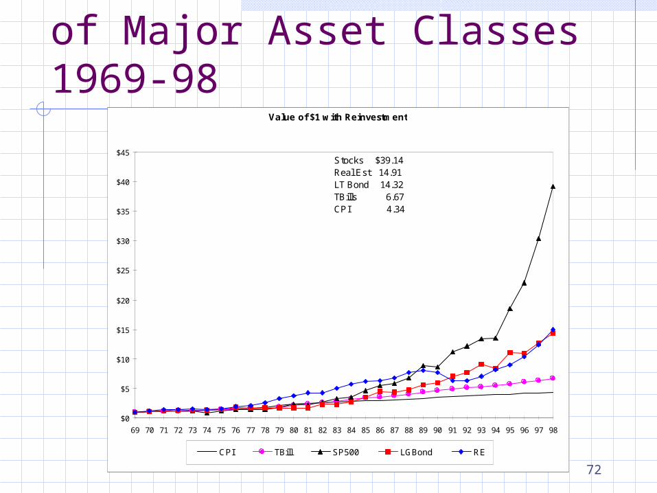
Historical Performance of Major Asset Classes 1969-98
Value of $1 with Reinvestment
$0
$5
$10
$15
$20
$25
$30
$35
$40
$45
69 70 71 72 73 74 75 76 77 78 79 80 81 82 83 84 85 86 87 88 89 90 91 92 93 94 95 96 97 98
CPI TBill SP500 LGBond RE
Stocks $39.14Real Est 14.91LT Bond 14.32TBills 6.67CPI 4.34
73
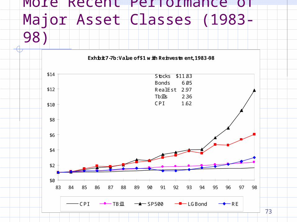
More Recent Performance of Major Asset Classes (1983-98)
Exhibit 7-7b: Value of $1 with Reinvestment, 1983-98
$0
$2
$4
$6
$8
$10
$12
$14
83 84 85 86 87 88 89 90 91 92 93 94 95 96 97 98
CPI TBill SP500 LGBond RE
Stocks $11.83Bonds 6.05Real Est 2.97Tbills 2.36CPI 1.62
74
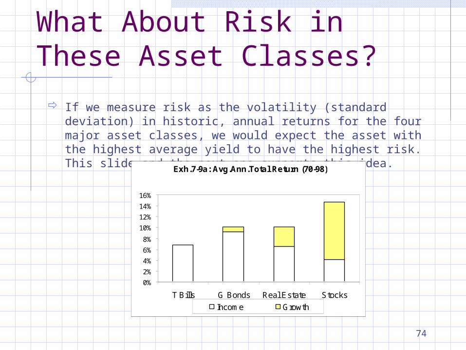
What About Risk in These Asset Classes?
If we measure risk as the volatility (standard deviation) in historic, annual returns for the four major asset classes, we would expect the asset with the highest average yield to have the highest risk. This slide and the next one supports this idea.
Exh.7-9a: Avg.Ann.Total Return (70-98)
0%
2%
4%
6%
8%
10%
12%
14%
16%
T Bills G Bonds Real Estate Stocks
Income Growth

75
Comparing “Risk” for the 4 Major Asset Classes
Exh.7-9b: Annual Volatility (70-98)
0%
2%
4%
6%
8%
10%
12%
14%
16%
18%
T Bills G Bonds Real Estate Stocks
76
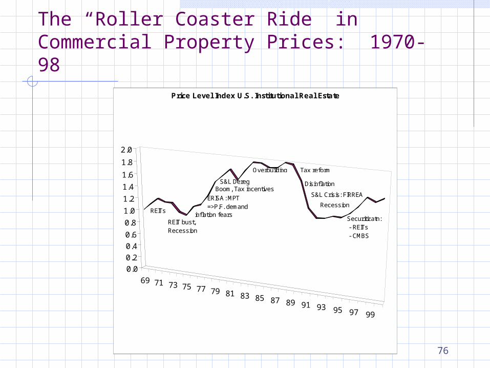
The “Roller Coaster Ride” in Commercial Property Prices: 1970-98
69 71 73 75 77 79 81 83 85 87 89 91 93 95 97 99
0.0
0.2
0.4
0.6
0.8
1.0
1.2
1.4
1.6
1.8
2.0
Price Level Index U.S. Institutional Real Estate
REITs
REIT bust,Recession
ERISA: MPT=>P.F. demand
inflation fears
Boom, Tax incentivesS&L Dereg
Overbuilding Tax reform
Disinflation
Recession
S&L Crisis: FIRREA
Securitizatn: - REITs - CMBS
Measuring Investment Performance
Module 7: Real Estate Investment Analysis
78
The Concept of “Returns”
Investors use the concept of returns to “quantify” or measure investment performance .
“Returns” refers to:Profits, measured as a percentage of the
investment amountWhat you’ve got minus what you had to begin
with as a proportion of what you had to begin withQuantitative return measures are necessary to:
Measure past performance (ex post or historical returns)
Express expectations about future performance (ex ante or expected returns)
79
Two Major Types of Return Measures
There are two major types of mathematical return definitions:Period-by-period returns
Simple holding period return (HPR)
Multiperiod returnsInternal rate of return (IRR)
80
Holding Period Returns (HPR)
Also known as “periodic returns,” holding period returns (HPR) measure what the investment grows to within each single period of time.
HPR assume all cash flows (or valuations) occur only at the beginning and end of the period of time with no intermediate cash flows.
Returns are measured separately over each of a sequence of regular and consecutive (relatively short) periods of time such as daily, monthly, quarterly, or annual return series.
HPR can be averaged across time to determine the “time-weighted” multiperiod return.
81
Two Ways to “Average” There are two different ways to calculate the “Average” of a data series and
each has its advantages and disadvantages, depending on the situation at hand. Arithmetic average = sum of the observations divided by the number of
observations Geometric average = nth root of the product of “1 plus each observation,”
minus 1 [(1+data1)x(1+data2)x…x(1+dataj)]^(1/j) –1
Arithmetic mean is always greater than the geometric mean, especially if the data are more volatile.
Arithmetic mean is a better estimate of central tendency than the geometric mean.
The income and appreciation components of the arithmetic mean sum to the arithmetic mean total return.
The geometric mean is a better indicator of the average growth rate over a time period because it recognizes compounding, if any.
The geometric mean is not affected by volatility in the data. The income and appreciation components of the geometric mean do not sum
to the geometric mean total return.
82
IRR as a Multiperiod Return Measure
How can we measure returns when the cash flows of an investment occur at more than two points in time?
The internal rate of return (IRR) is the most common multiperiod return measure.
We usually quote the IRR as a per annum (per year) rate.
The IRR is a dollar-weighted return because it reflects the effect of having different amounts of money invested at different periods of time during the lifetime of an investment.
83
Advantages and Disadvantages of Periodic and Multiperiod Return Measures
ADVANTAGES OF PERIOD-BY-PERIOD (TIME-WEIGHTED) RETURNS: ALLOW YOU TO TRACK PERFORMANCE OVER TIME, SEEING WHEN INVESTMENT IS DOING
WELL AND WHEN POORLY. ALLOW YOU TO QUANTIFY RISK (VOLATILITY) AND CORRELATION (CO-MOVEMENT) WITH
OTHER INVESTMENTS AND OTHER PHENOMENA. ARE FAIRER FOR JUDGING INVESTMENT PERFORMANCE WHEN THE INVESTMENT
MANAGER DOES NOT HAVE CONTROL OVER THE TIMING OF CASH FLOW INTO OR OUT OF THE INVESTMENT FUND (E.G., A PENSION FUND).
ADVANTAGES OF MULTI-PERIOD RETURNS:
DO NOT REQUIRE KNOWLEDGE OF MARKET VALUES OF THE INVESTMENT ASSET AT INTERMEDIATE POINTS IN TIME (MAY BE DIFFICULT TO KNOW FOR REAL ESTATE).
GIVES A FAIRER (MORE COMPLETE) MEASURE OF INVESTMENT PERFORMANCE WHEN THE INVESTMENT MANAGER HAS CONTROL OVER THE TIMING AND AMOUNTS OF CASH FLOW INTO AND OUT OF THE INVESTMENT VEHICLE (E.G., PERHAPS SOME "SEPARATE ACCOUNTS" WHERE MGR HAS CONTROL OVER CAPITAL FLOW TIMING, OR A STAGED DEVELOPMENT PROJECT).
NOTE: BOTH HPR AND IRR ARE WIDELY USED IN REAL ESTATE INVESTMENT
ANALYSIS
84
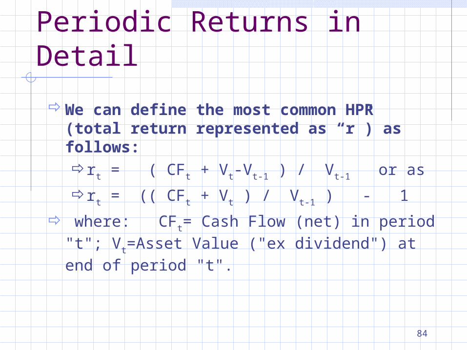
Periodic Returns in Detail
We can define the most common HPR (total return represented as “r”) as follows: rt = ( CFt + Vt-Vt-1 ) / Vt-1 or as
rt = (( CFt + Vt ) / Vt-1 ) - 1
where: CFt= Cash Flow (net) in period "t";
Vt=Asset Value ("ex dividend") at end of period "t".
85
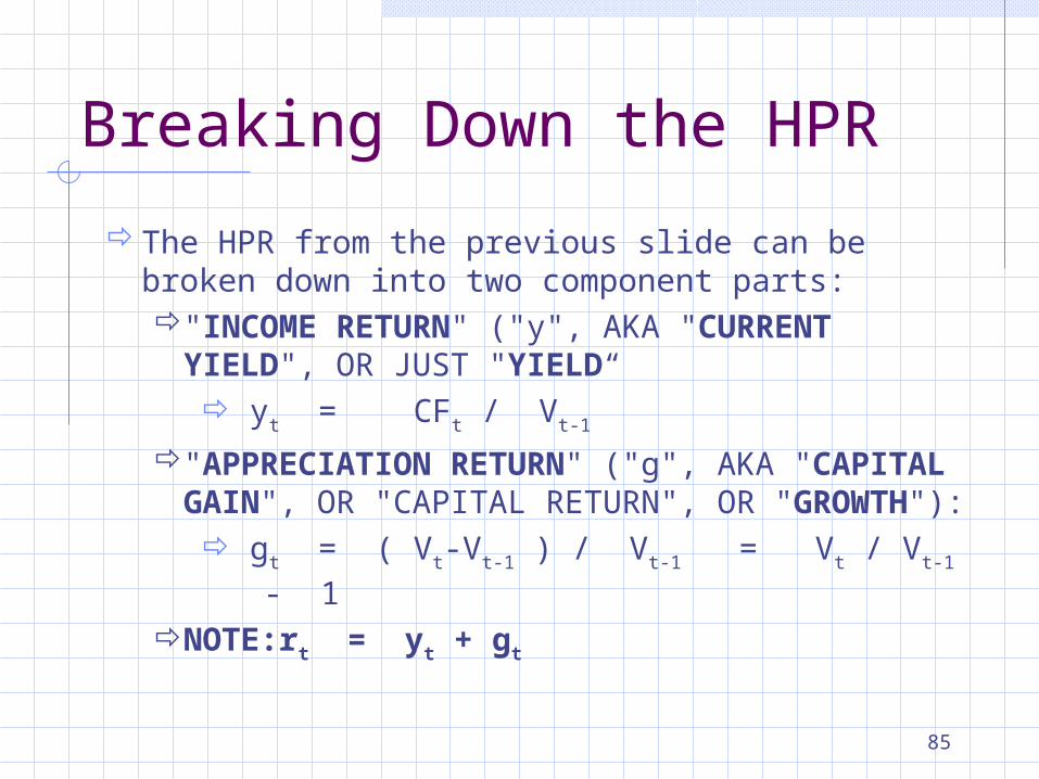
Breaking Down the HPR
The HPR from the previous slide can be broken down into two component parts:"INCOME RETURN" ("y", AKA "CURRENT YIELD",
OR JUST "YIELD“ yt = CFt / Vt-1
"APPRECIATION RETURN" ("g", AKA "CAPITAL GAIN", OR "CAPITAL RETURN", OR "GROWTH"): gt = ( Vt-Vt-1 ) / Vt-1 = Vt / Vt-1 - 1
NOTE: rt = yt + gt
86
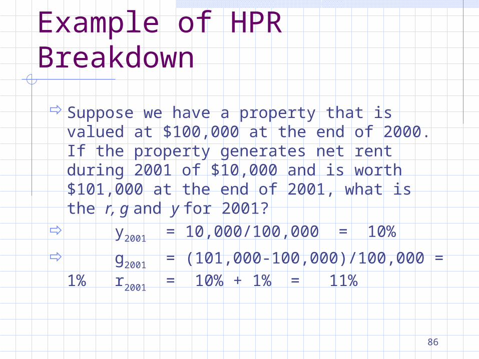
Example of HPR Breakdown
Suppose we have a property that is valued at $100,000 at the end of 2000. If the property generates net rent during 2001 of $10,000 and is worth $101,000 at the end of 2001, what is the r, g and y for 2001?
y2001 = 10,000/100,000 = 10%
g2001 = (101,000-100,000)/100,000 = 1%r2001
= 10% + 1% = 11%
87
MultiPeriod Returns in Detail
When we wish to quantify the return of an investment earned over a multiperiod span of time we have two options: Time-weighted average return (arithmetic or geometric average) Dollar-weighted average return (such as the Internal Rate of
Return defined in the previous module) Time-weighted returns ignore the amount of money invested
in the investment during the individual time periods and any cash flows that occur within the individual time periods.
Dollar-weighted returns take these issues into consideration. The type of measure we should used varies with the type of
situation we are trying to evaluate. We will see a common “hybrid” of these two types when we review the NCREIF Property Index later in this presentation.
88
Measuring Risk in Returns
Intuitively, risk in investment analysis refers to the possibility of not making the expected return.
We can measure risk by the standard deviation of the future return possibilities. We call this measure “volatility.”
The larger the standard deviation, the greater the volatility or risk.
89
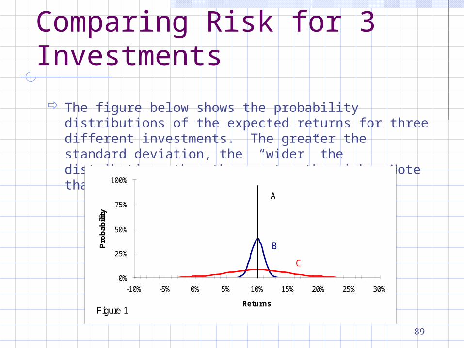
Comparing Risk for 3 Investments
The figure below shows the probability distributions of the expected returns for three different investments. The greater the standard deviation, the “wider” the distribution, thus the greater the risk. Note that the expected return for each is 10%.
0%
25%
50%
75%
100%
-10% -5% 0% 5% 10% 15% 20% 25% 30%
Returns
Pro
bab
ility
A
B
C
Figure 1
90
The Risk-Return Tradeoff
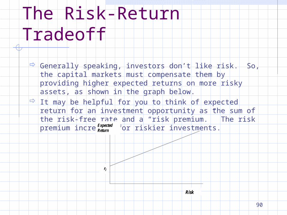
Generally speaking, investors don’t like risk. So, the capital markets must compensate them by providing higher expected returns on more risky assets, as shown in the graph below.
It may be helpful for you to think of expected return for an investment opportunity as the sum of the risk-free rate and a “risk premium.” The risk premium increases for riskier investments.
Risk
ExpectedReturn
rf
91
One last item … the NCREIF Index
The most widely referenced measure of returns to commercial real estate investment is the NCREIF Property Index (NPI).
NPI is published quarterly by the National Council of Real Estate Investment Fiduciaries and is based on regular appraisals of a large sample (2500+) properties worth about $70 billion located all across the U.S.
The NPI is broken down by property type and geographic region: office, retail, industrial, apartment; East, Midwest, South, and West.
The NPI is a uniquely defined time-weighted return measure that accounts for the fact that the index is published quarterly, but real estate investments generate cash flows on a monthly basis.
92
NPI formula
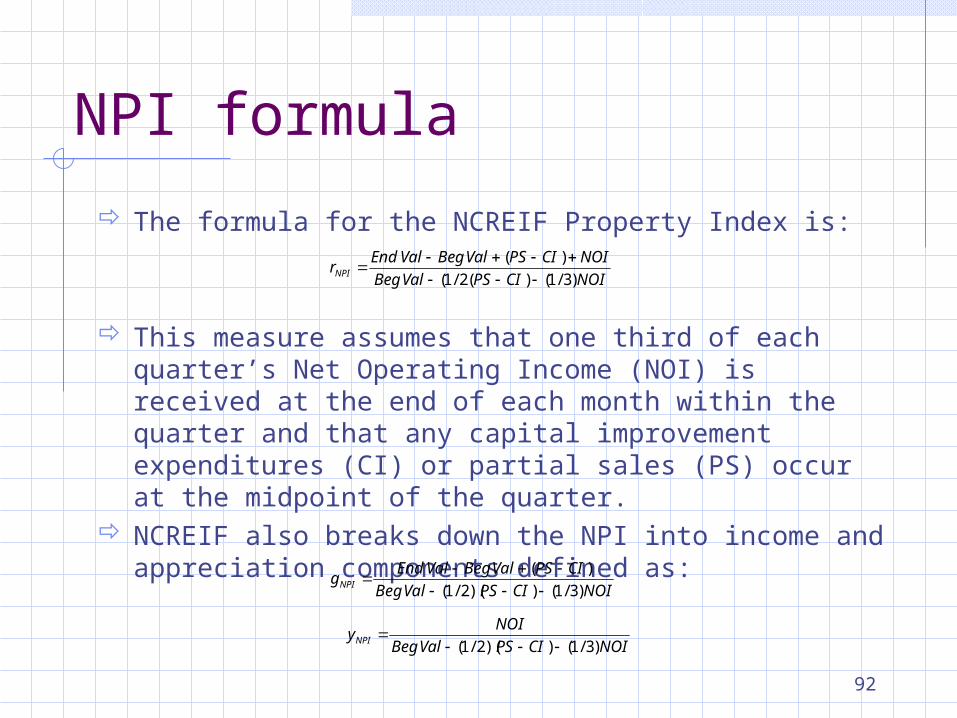
The formula for the NCREIF Property Index is:
This measure assumes that one third of each quarter’s Net Operating Income (NOI) is received at the end of each month within the quarter and that any capital improvement expenditures (CI) or partial sales (PS) occur at the midpoint of the quarter.
NCREIF also breaks down the NPI into income and appreciation components defined as:
NOICIPSValBeg
NOICIPSValBegValEndrNPI )3/1()(2/1(
)(
NOICIPSValBeg
CIPSValBegValEndgNPI )3/1())(2/1(
)(
NOICIPSValBeg
NOIyNPI )3/1())(2/1(
Discounted Cash Flow and NPV
Module 8: Real Estate Investment Analysis
94
Reviewing the Relationship between Returns and Values
In the previous module, we spent considerable time discussing the concept of returns and how important they are to real estate investors.
In order to actually earn returns, of course, investors must purchase investments.
Our task in this chapter is to consider how investors determine how much they will are willing to pay for an investment that is expected to generate cash flows.
Expected return serves as the link between cash flows and values.
The tool we will use for evaluating values of specific investment opportunities in light of expected returns is called Discounted Cash Flow Valuation (DCF).
95
The Discounted Cash Flow Valuation Procedure
The discounted cash flow valuation (DCF) procedure consists of three steps:Forecast the expected future cash
flowsAscertain the required total returnDiscount the cash flows to present
value at the require rate of return.
96
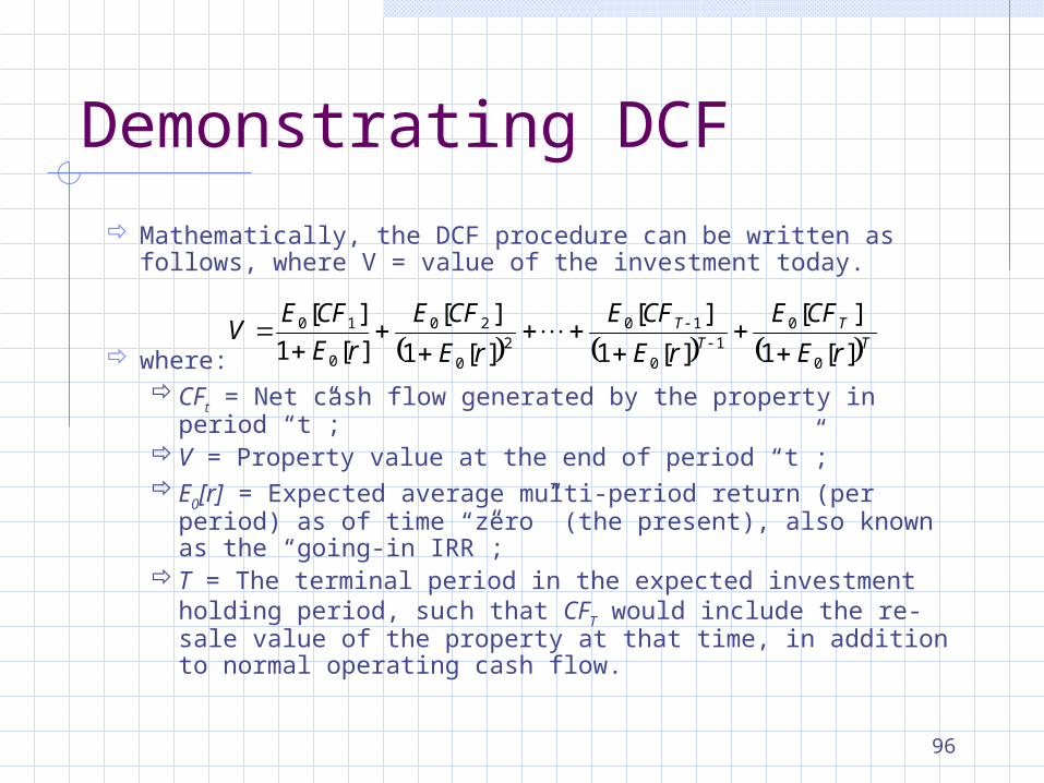
Demonstrating DCF
Mathematically, the DCF procedure can be written as follows, where V = value of the investment today.
where:CFt = Net cash flow generated by the property in period “t”;V = Property value at the end of period “t”;E0[r] = Expected average multi-period return (per period)
as of time “zero” (the present), also known as the “going-in IRR”;
T = The terminal period in the expected investment holding period, such that CFT would include the re-sale value of the property at that time, in addition to normal operating cash flow.
TT
TT
rE
CFE
rE
CFE
rE
CFE
rE
CFEV
][1
][
][1
][
][1
][
][1
][
0
01
0
102
0
20
0
10
97
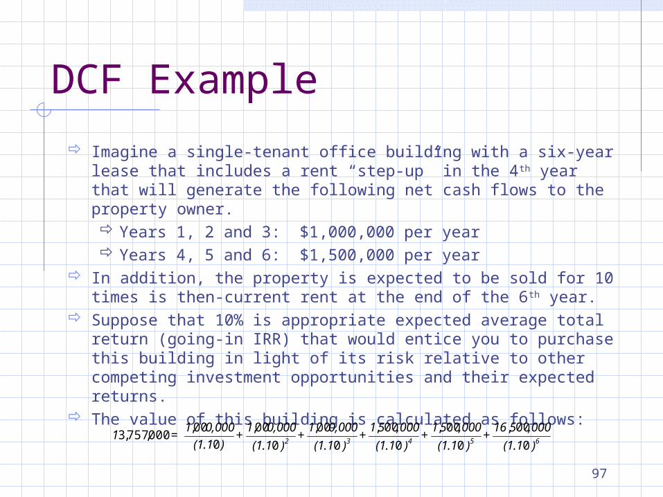
DCF Example
Imagine a single-tenant office building with a six-year lease that includes a rent “step-up” in the 4th year that will generate the following net cash flows to the property owner. Years 1, 2 and 3: $1,000,000 per year Years 4, 5 and 6: $1,500,000 per year
In addition, the property is expected to be sold for 10 times is then-current rent at the end of the 6th year.
Suppose that 10% is appropriate expected average total return (going-in IRR) that would entice you to purchase this building in light of its risk relative to other competing investment opportunities and their expected returns.
The value of this building is calculated as follows:
)(1.1
,000516+
)(1.1
,00051+
)(1.1
,00051+
)(1.1
0,0001+
)(1.1
0,0001+
)(1.1
0,0001 = 1
65432 0
00,
0
00,
0
00,
0
00,
0
00,
0
00,000,757,3
98
Choosing the Right Discount Rate in DCF
In DCF calculations, larger discount rates result in smaller present values.
Relatively small errors in the discount rate (measured in basis points) can cause dramatic errors in value calculations (measured in dollars).
Keep in mind that different cash flows in the DCF model may pose different risk levels (forecasting rent with existing leases is “easier” than trying to forecast rent from potential leases with unknown tenants), thus requiring different discount rates or a “blended” rate that takes into account the variation in risk.
Using a blended rate (which is what we normally do) is not such a bad shortcut if that’s the way market participants really approach the valuation process, even if it is not technically correct.
99
Two Common DCF “Shortcuts”
While DCF analysis is considered to be the theoretically correct approach to valuation, there may be times when other approaches are acceptable.
Two shortcut approaches commonly used in real estate are:Direct Capitalization Technique
V=I/R, where V is value, I is net income, and R is the overall capitalization rate discussed in Chapter 1 of the textbook (a yield measure, not a total return measure).
Gross Income Multiplier TechniqueV=GIxGIM, where V is value, GI is gross income, and
GIM is the gross income multiplier prevailing in the market.
Shortcuts can be useful in practice, but we should realize that they may omit important information that could be relevant to the valuation decision.

100
Watch out for the garbage truck!
No matter how sophisticated the DCF approach looks and no matter if the math “adds up,” the valuation can be no better than the quality of the inputs: cash flow forecast and discount rate assumptions.
In other words: Garbage in, Garbage Out
101
Making the Investment Decision with NPV
We discussed the concept of Net Present Value and how it could be used as a decision tool in the module addressing “Present Value Mathematics” or “Time Value of Money.”
The NPV Rule says that an investor will choose to accept those investment opportunities that are expected to generate a present value of cash inflows equal to or greater than the present value of cash outflows, with present values reflecting the investor’s require rate of return.
When faced with mutually exclusive investment choices, we should choose the one with the largest positive NPV.
The NPV Rule is consistent with the overall objective of all investors: Wealth Maximization
Due to competition, we would expect all investment opportunities to reflect a zero NPV on a market value basis. Of course, we all hope to find deals in which the rest of the market is “mispricing” the opportunity, allowing us to identify projects that offer positive NPV on an investment value basis make abnormal returns on.
102
What about the IRR as a Decision Tool?
Recall that we defined Internal Rate of Return (IRR) as the discount rate which sets the NPV of an investment opportunity equal to zero.
If the calculated IRR of an investment opportunity is greater than or equal to the required rate of return, then the investor should accept the opportunity.
The trouble with using IRR as a decision rule is that it does not help us distinguish between mutually exclusive projects because it ignores their scale (amount of dollars involved). Furthermore, there are some situations when IRR cannot be calculated and still other situations when there can be multiple IRRs.
Thus, using the IRR as the “hurdle rate” for making investment decision can lead to choices that do not “maximize wealth.”
Projecting Operating and Reversion Cash Flows
Module 9: Real Estate Investment Analysis
104
Property Level vs. Investor Level Cash Flows
Now that we understand the theoretical approach to making real estate investment decisions using DCF and NPV, our attention in this module focuses on how to project or forecast the cash flows.
Cash flow consists of two major components in most real estate investments:Cash flow from operations Cash flow from sale of the asset at the end of
holding periodWe will focus on “property level” before tax cash
flows for now, but later we will consider “investor level” cash flows that reflect taxes and financing.
105
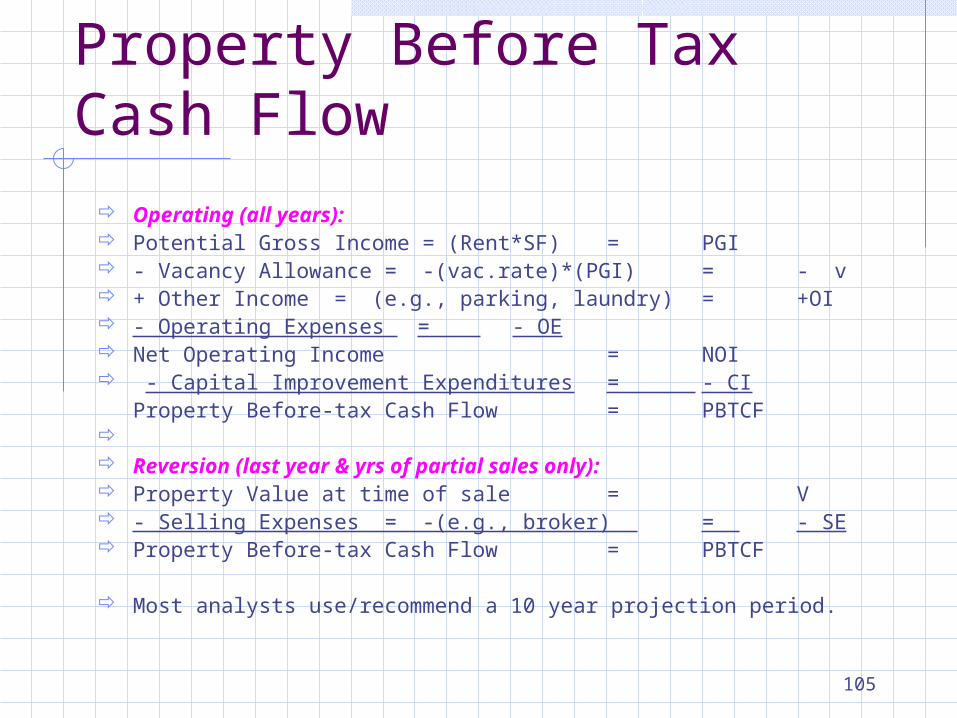
Property Before Tax Cash Flow
Operating (all years): Potential Gross Income = (Rent*SF) = PGI - Vacancy Allowance = -(vac.rate)*(PGI) = - v + Other Income = (e.g., parking, laundry) = +OI - Operating Expenses = - OE Net Operating Income = NOI - Capital Improvement Expenditures = - CI
Property Before-tax Cash Flow = PBTCF Reversion (last year & yrs of partial sales only): Property Value at time of sale = V - Selling Expenses = -(e.g., broker) = - SE Property Before-tax Cash Flow = PBTCF
Most analysts use/recommend a 10 year projection period.
106
Some Issues in PBTCF
How do we forecast vacancy (v)?Vac = (vac months)/(vac months + rented months) in typical
cycle;Look at typical vac rate in rental mkt, or history in subject
bldg. How do we forecast resale value (“reversion”, V at end)?
Divide Yr.11 NOI by “going-out” (terminal) cap rate. What should be the typical relationship between the going-in
cap rate and the going-out cap rate?. . . Usually going-out going-in (older bldgs have less growth & more
risk), esp. if little capital imprvmt expdtrs have been projected
107
Some More Issues in PBTCF
Operating Expenses include: Fixed:
Property TaxesProperty InsuranceSecurityManagement
Variable:Maintenance & RepairsUtilities (not paid by tenants)
NOTE: OE do not include: income taxes or depreciation expense, but must include mgt expense even if self-managed. Why? . . . Opportunity cost, “apples-to-apples” comparison with
alternative investments that you don’t have to manage yourself.
108
Yet more issues…..
Capital Expenditures include: Leasing costs:
Tenant build-outs or improvement expenditures (“TIs”)Leasing commissions to brokers
Property Improvements:Major repairsReplacement of major equipmentMajor remodeling of building, ground & fixtures
Expansion of rentable area
109
Discount Rates
The discount rate used to convert cash flows into present values is:is a multiperiod, dollar weighted average total
return expected by the investor in the form of a “going-in” IRR
composed of the riskfree rate plus a risk premium that accounts for risk in the cash flow projection
equal to the return investors could typically earn on average in other investments of similar risk to the subject property
derived from the capital markets.
110
A few thoughts on risk and discount rates for DCF…
Risk is in the object not in the beholder.Property "X" has the same risk for Investor "A" as
for Investor "B".Therefore, oppurtunity cost of capital is same for
“A” & “B” for purposes of evaluating NPV of investment in “X” (same discount rate). Unless, say, “A” has some unique ability to alter the risk of X’s future CFs. (This is rare: be skeptical of such claims!)
111
How do we determine the discount rate to use in DCF?
Usually a single ("blended") multi-year rate is OK for valuation and investment analysis ("going-in IRR"). One source of info is direct surveysdirect surveys of market
participants (see www.korpacz.com)Another source is historical evidence such as NPI.historical evidence such as NPI.
Survey data tends to average about 200 bps > Historical data.
112
Typical Going-In IRRs
For high quality ("class A", "institutional quality") income property:10% - 12%, stated 8% - 10%, realistic
Lower quality or more risky income property (e.g., hotels, class B commercial, turnarounds, "mom & pops"):12% - 15%
Raw land (speculation):15% - 30%
113
How can we “back out” implied discount rates from observed “cap rates?”
Recall that we defined the cap rate asNOI / V CF / V = y.
Therefore, from market transaction data...Observe prices (V)Observe NOI of sold propertiesObserve "cap rates" = NOI / V.Compute: r = y + g cap rate + g.So, we can get an idea what the market's expected total
return (discount rate) is for different types of properties by observing the cap rates at which they are sold and then making reasonable assumptions about growth expectations (g).

More Microlevel Valuation Ideas
Module 10: Real Estate Investment Analysis
115
What makes real estate different from traditional corporate investment decisions?
The investment decision tools considered thus far in this course are really the same tools that any investor should use to analyze any type of investment opportunity (real estate or any other type).
In corporate finance courses, the tools we have been using (DCF, NPV, IRR) are called “capital budgeting tools.”
Three characteristics of real estate that differ from traditional corporate investment decisions include: A well-functioning market exists for real estate assets (unlike
assembly lines or microchip fabrication machines) The market, though well-functioning, is not as “informationally
efficient” as the market for publicly traded securities such as stocks and bonds.
In addition to the private real estate asset market, a parallel, public real estate market exists (REITs) that implies that there may be arbitrage opportunities for real estate assets.
116
Investment Vs. Market Value
Market value is the expected price at which an asset can be sold in the current market If we actually sold an asset, the observed price has an equal
probability of being above or below the “expected price.” Appraisers sometimes say that market value is the value of a
property to the “typical buyer” in the market. In this sense, market value can be regarded as “opportunity
value,” or, “the most probable price.” Investment value is the value of an asset to a particular owner,
reflecting that owner’s unique situation. In most corporate capital budgeting decisions, there is no well-
functioning market for the underlying physical assets, so NPV decisions are based on investment value.
In real estate, the existence of the real estate asset market means that both investment value and market value can be (and should be) evaluated when making investment choices.
117
Investment Value
Investment value is measured by considering: The cash flows expected to result under the particular
owner’s management and operation of the asset, as well as the owner’s income tax situation.
The cash flows on the right-hand side of the DCF formula may differ from one investor to another!
The discount rate that accounts for the risk inherent in the cash flow forecast and the time value of money.
Usually, the discount rate used in the DCF formula should be the same for a particular property no matter who the investor is, since all investors are competing in the same capital market.
118
Using IV and MV to define NPV
The NPV rule, in general, says we should accept only those projects with “non-negative” NPV and, if faced with a mutually exclusive choice, we should choose the project with the greatest NPV.
For a buyer, NPV is equal to “IV – MV”Buy it if it is worth more to you than it is to the
typical buyer! For a seller, NPV is equal to “MV – IV”
Sell if if it is worth more to the “typical buyer” than it is to you!
119
Can Positive NPV Projects Really Exist?
In a perfectly competitive market with no information asymmetries or other imperfections, competition would force IV=MV for all investors for all assets, and everyone’s NPV would be zero for all transactions. If IVbuyer = IVseller = MV, then NPV = zero for both
buyer and seller.This is what finance professors are talking about
when they lecture on “efficient market theory.”Don’t forget that “zero NPV” deals are still good!
But, the real estate market is not so perfect and it is possible for real estate deals to result in positive NPV for either the buyer, the seller, or both simultaneously!
120
How can we get positive NPV?
We have already established that most investors face the same discount rate (the opportunity cost of capital), so the only way NPV can be positive for the buyer, the seller, or both in the same deal is if the cash flows are different depending on who owns the property.
Thus, the characteristics of the owner can affect NPV if the characteristics affect the cash flow projection.
Characteristics that might affect cash flow include: Owner’s income tax status Owner’s long-term use plan for the property Owner’s management ability (economies of scale, specialized skills,
etc.) Transaction costs may vary across owners Information asymmetries may result in different cash flow projections
across owners. Negotiating skills differ across owners. Time constraints and horizons may differ across owners.
121
Arbitrage opportunities between the public and private real estate asset markets.
When the same asset is traded in two different markets at two different prices, an opportunity exists to “buy low” in one market and “sell high” in the other, or arbitrage.
Researchers (Downs, Geltner, Giliberto & Mengden, Gyourko & Keim, Graff & Young, Ling & Naranjo, Liu, etc.) have examined whether it is possible to “arbitrage” between the private real estate asset market (direct ownership of buildings) and the public real estate asset market (REITs and other publicly traded assets.)
The idea is that sometimes these two markets may not identically “price” real estate cash flows, so investors who can spot the opportunities may have a chance to arbitrage.
The results of this research are mixed, and it is not clear that the profits from arbitrage would be large enough to cover transaction costs in the long run.
Capital Structure
Module 11: Real Estate Investment Analysis
123
Introduction to Capital Structure Theory
The term capital structure refers to the relative proportion of equity (investor funds) and debt (lender funds) in a real estate investment.
Many assets in the real estate asset market are funded with a combination of debt and equity.Real estate assets are well-suited as collateral for debt,
so lenders are accustomed to making real estate loans. Investors like the way debt allows them to magnify or
“lever” the amount of physical capital they control. (They can buy more real estate with the same amount of investor funds if they combine these funds with lender funds!)
124
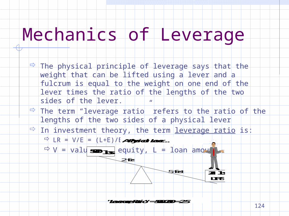
Mechanics of Leverage
The physical principle of leverage says that the weight that can be lifted using a lever and a fulcrum is equal to the weight on one end of the lever times the ratio of the lengths of the two sides of the lever.
The term “leverage ratio” refers to the ratio of the lengths of the two sides of a physical lever
In investment theory, the term leverage ratio is: LR = V/E = (L+E)/E V = value, E = equity, L = loan amount
500lbs
200lbs
A Physical Lever...
"Leverage Ratio" = 500/200 = 2.5
LIFTS
5 feet
2 feet
125
Effects of Financial Leverage
When an investor combines equity funds with borrowed funds to leverage an investment, the leverage increases the:Expected return to the equity investorRisk of the investment to the equity investor
126
Example of the effect on expected return
Consider a property that can be purchased for $100,000 today that will increase in value by 2% during the next year and will generate $8,000 during the year in cash flow for a total return of 10%.
If an investor buys this building with $100,000 of equity funds, the return on his equity investment will be 10%
10,000/100000 = .10 If an investor buys this building with $40,000 in
equity and $60,000 in debt at 8% interest (interest only loan), the return on his equity investment is 13%
(10,000-4,800)/40000 = .13
127
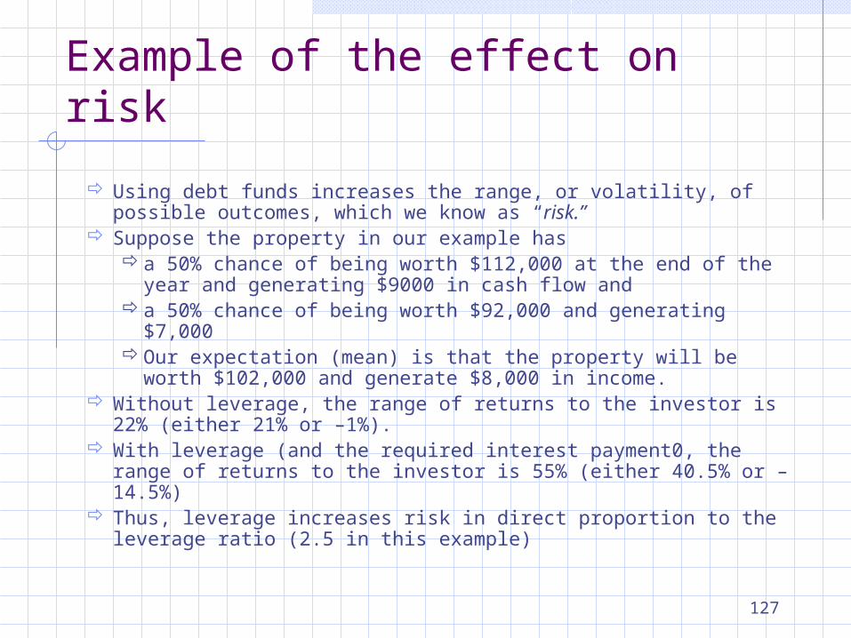
Example of the effect on risk
Using debt funds increases the range, or volatility, of possible outcomes, which we know as “risk.”
Suppose the property in our example has a 50% chance of being worth $112,000 at the end of the
year and generating $9000 in cash flow anda 50% chance of being worth $92,000 and generating
$7,000Our expectation (mean) is that the property will be worth
$102,000 and generate $8,000 in income. Without leverage, the range of returns to the investor is 22%
(either 21% or –1%). With leverage (and the required interest payment0, the range
of returns to the investor is 55% (either 40.5% or –14.5%) Thus, leverage increases risk in direct proportion to the
leverage ratio (2.5 in this example)
128
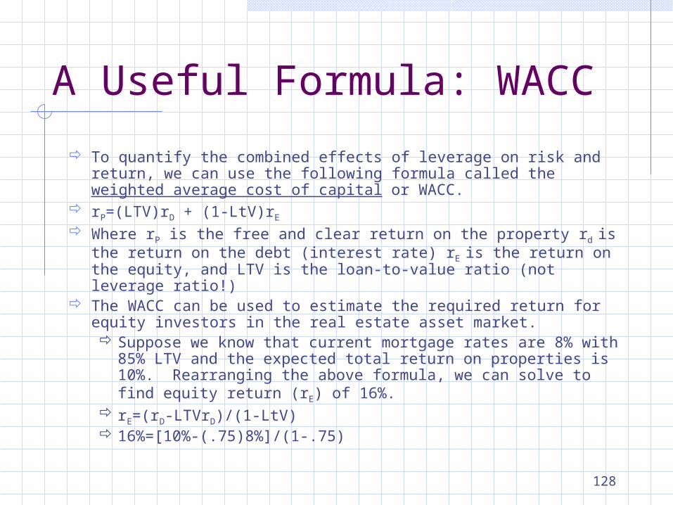
A Useful Formula: WACC
To quantify the combined effects of leverage on risk and return, we can use the following formula called the weighted average cost of capital or WACC.
rP=(LTV)rD + (1-LtV)rE
Where rP is the free and clear return on the property rd is the return on the debt (interest rate) rE is the return on the equity, and LTV is the loan-to-value ratio (not leverage ratio!)
The WACC can be used to estimate the required return for equity investors in the real estate asset market. Suppose we know that current mortgage rates are 8% with
85% LTV and the expected total return on properties is 10%. Rearranging the above formula, we can solve to find equity return (rE) of 16%.
rE=(rD-LTVrD)/(1-LtV) 16%=[10%-(.75)8%]/(1-.75)
129
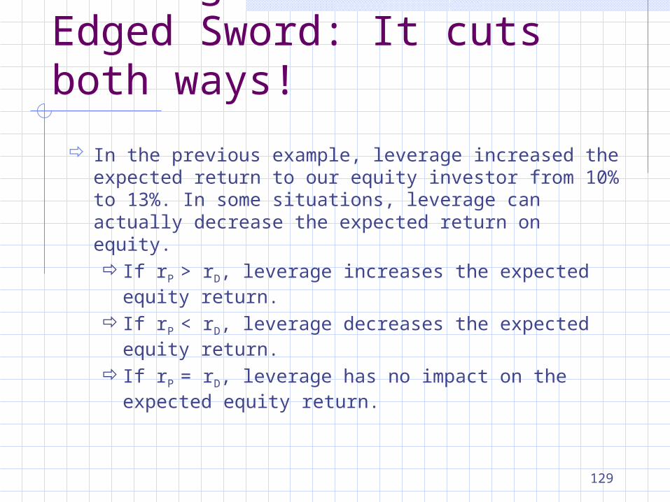
Leverage is a Two-Edged Sword: It cuts both ways!
In the previous example, leverage increased the expected return to our equity investor from 10% to 13%. In some situations, leverage can actually decrease the expected return on equity. If rP > rD, leverage increases the expected equity
return. If rP < rD, leverage decreases the expected equity
return. If rP = rD, leverage has no impact on the expected
equity return.
Income Tax Considerations
Module 12: Real Estate Investment Analysis

131
Uncle Sam Wants Yours!
So far in this course we have ignored the impact of income taxes on the investment decision.
For pension funds, life insurance companies and other similar entities for whom investment returns are not subject to taxation, ignoring taxes is perfectly legitimate.
For the rest of us, income taxes are an important consideration that can dramatically affect the investment decision.
132
PBTCF vs Equity ATCF
The property level before tax cash flow used in the DCF model thus far in this course is often significantly different from the property owner’s “equity after tax cash flows” due to accrual based IRS rules relating to:Depreciation – a non-cash expense that reflects the
accrual of losses in property value over timeCapital expenses – a cash item, but IRS requires
depreciation over the life of the improvementDebt amortization – mortgage payments include
principal and interest, but only the interest portion is an expense, since principal reduction just moves money from one pocket to the other.
133
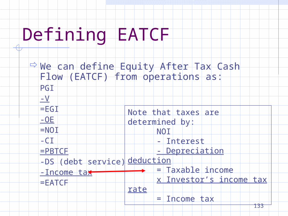
Defining EATCF
We can define Equity After Tax Cash Flow (EATCF) from operations as:PGI-V=EGI-OE=NOI-CI=PBTCF-DS (debt service)-Income tax=EATCF
Note that taxes are determined by:
NOI- Interest- Depreciation deduction= Taxable incomex Investor’s income tax
rate= Income tax
134
Defining After Tax Reversion Cash Flow (ATRCF)
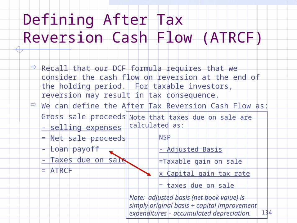
Recall that our DCF formula requires that we consider the cash flow on reversion at the end of the holding period. For taxable investors, reversion may result in tax consequence.
We can define the After Tax Reversion Cash Flow as:Gross sale proceeds- selling expenses= Net sale proceeds- Loan payoff- Taxes due on sale= ATRCF
Note that taxes due on sale are calculated as:
NSP
- Adjusted Basis
=Taxable gain on sale
x Capital gain tax rate
= taxes due on sale
Note: adjusted basis (net book value) is simply original basis + capital improvement expenditures – accumulated depreciation.
135
Other Tax Concepts: Original Tax Basis
Original (initial) Tax Basis - the costs of acquiring property by purchase, including everything of value given in exchange (excluding items deductible as current operating expenses)cashdebt legal work title insuranceother fees or charges
136
Other Tax Concepts: Allocating the Tax Basis
Allocating the Tax Basis - the initial basis is allocated between the costs of land and the costs of improvements in a manner which reflects their respective market values The portion attributable to improvements is often called the
Depreciable Basis
Three methods for allocating the tax basis:specify the price of each component in the
purchase contractuse the ratio of land value to building value as
employed by the tax assessorhave an appraiser estimate the relative values of
land and buildings
137
Other Tax Concepts: Adjusting the Basis
Adjusting the Basis - three main topics to consider: Cost Recovery Allowance (depreciation)Capital ImprovementsPartial Sale
138
Cost Recovery Allowance (depreciation)
Cost Recovery Allowance (depreciation) our federal government taxes income, not wealth (supposedly) to allow investors to recover their investment capital (wealth) without
paying taxes on it (again), the IRS permits taxpayers to deduct from otherwise taxable income an allowance for recovery of invested capital
applies to virtually all investment in assets held for business or income purposes, including property improvements, but excluding land
depreciable life is the phrase commonly used to refer to the period over which costs for such assets may be recovered residential income property: 27.5 years (80%+ of gross rents from
residential tenants) non-residential income property: 39 years land improvements (walks, roads, sewers, gutters, fences): 15 years personal property such as appliances, automobiles: 5 years personal property such as officer furniture, fixtures, equipment: 7 years
139
Computing the Depreciation Deduction
The annual Cost Recovery Allowance (depreciation deduction) is prorated by months for property owned for less than a full calendar year mid-month convention - during the month a property is placed into
service, and the month when a property is removed from service, the tax payer may claim only half of the monthly allowance.
Example: consider a taxpayer who acquires a residential income property on March 2, 2001, and operates it until she sells it on November 29, 2003. The depreciable basis is $240,000. The annual depreciation or recovery allowance is: 240,000/27.5 = $8,727. The first and last years of ownership, however, require use of the mid-month convention.
2001: 9.5 x (8,727/12) = $6,909 2002: full year $8,727 2003: 10.5 x (8,727/12) = $7,636 Total $23,272 Note: A “half-year convention” applies to personal property
140
How do Capital Improvement Expenditures affect taxable income?
Capital Improvements when an investor expends additional funds to improve a property,
the IRS may classify those expenditures as capital improvements rather than operating expenses
expenditures that add to the value or extend the life span of the improvements are capital improvements
expenditures that only maintain the properties operating condition are current operating expenses
whereas operating expenses are deductible in the year they are incurred, capital improvements must be deducted via cost recovery allowances
of course, investors would generally prefer to classify all expenditures as operating expenses to reduce their taxable income in the year the expenses are incurred
Partial Sale when a portion of a property is sold, the tax basis must be reduced
by the portion of the total basis attributable to the part sold
141
What discount rate should we use for After-Tax DCF?
Now that we can project cash flows on an after-tax basis, we can apply the DCF formula to make investment decisions using the NPV rule.
Of course, we have to use the appropriate discount rate to use the DCF correctly.
When the property we are considering “trades” in a reasonably competitive market, the appropriate discount rate is the opportunity cost of capital.