Embed Size (px)
Citation preview
Real Estate Investment Trusts and Seasonal Volatility:
A Periodic GARCH Model
Marc Winniford* Duke University
Durham, NC Spring 2003
* Marc Winniford will graduate from Duke University in Spring 2004 with a Bachelor of Science in Economics and Mathematics. During the summers Marc has worked as a Financial Planner at Morgan Stanley and as an Equity Research Analyst at Credit Suisse First Boston. He plans to eventually pursue a Ph.D. in Economics.

2
Acknowledgement
I would like to thank my independent study mentor, Professor Tower, for his support and
guidance throughout the semester. I am also thankful for the feedback and assistance from
Professor Bray and the advice and helpful conversation with Professor Bollerslev. I am most
grateful to Alan Bester whose excellent teaching and enthusiasm for econometrics got me
interested in the subject. He continues to encourage me in my studies and has given me
invaluable advice and help with the topic and analyses in this paper. Finally, I would like to
thank my parents, Michael and Carol Winniford, for their love and support.
3
Abstract
Real Estate Investment Trusts (REITs) are correlated with the stock and real estate
markets; both of which exhibit seasonal fluctuations. In this study, key factors that influence the
seasonal volatility of Equity REIT (EREIT) returns are analyzed, and EREIT seasonal volatility
is modeled using a periodic generalized autoregressive conditional heteroskedasticity (P-
GARCH) model. EREIT returns are found to exhibit more pronounced seasonal volatility
patterns than the general stock market. EREITs show increased overall volatility in April, June,
September, October and December along with a greater sensitivity to news arrival in the summer
months. The results provide a more complete description of EREIT volatility patterns that can
be used as a framework for those involved in trading EREITs or EREIT options. The study also
establishes the P-GARCH model as a useful tool for modeling EREIT volatility.
4
1. Introduction
Real Estate Investment Trusts (REITs) are publicly traded investment companies that
invest in real estate properties and mortgages. REITs are generally classified into two broad
categories; Equity REITS (EREITs) invest at least 75% of their total assets in income producing
real estate properties, and mortgage REITs (MREITs) invest at least 75% of their total assets in
residential or commercial mortgages. REITs are a unique asset because of their dependence on
the stock, bond and real estate markets. Most previous research has focused on EREITs because
they make up 85% of all publicly traded REITs. From 1992 to 2003 EREITs have grown in
market capitalization from just under $11 billion to over $175 billion, as a result they are
becoming a more common part of an investors portfolio and are more frequently traded. It is
therefore important that their price movements be understood and that a comprehensive picture
of the return and volatility structure of EREITs be available.
In this study, key factors that influence the seasonal volatility of EREIT returns are
analyzed, and EREIT seasonality is modeled using a periodic generalized autoregressive
conditional heteroskedasticity (P-GARCH) model. The P-GARCH model accommodates a
seasonal structure in the volatility of EREITs that brings the residual series closer to normality.
The results of this study provide a more complete description of EREIT volatility and
interactions of EREITs with other markets; this could be useful in options trading and for those
investing in EREITs or adding them to a portfolio. The study also establishes the P-GARCH
model as a useful tool for modeling EREIT volatility processes.
2. Past Research
Past research on EREITs provides insight into the complex interactions between EREITs
and the stock, real estate and interest rate markets, and the possible sources of EREIT
5
seasonality. Most studies have focused on the influence of stock market and bond market factors
on EREIT returns. Peterson and Hsieh (1997) examine EREIT returns using the five-factor
model of Fama and French (1993). Fama and French found that the average returns on U.S.
common stock can be explained by size (price x shares outstanding), book-to-market ratio, the
term premium of interest rates, the default risk premium of interest rates, and a market factor.
Peterson and Hsieh argued that because EREIT shares trade on the major stock exchanges just
like common stocks, this model could also be applied to EREITs. The two interest rate factors in
the model are used to capture the portion of EREIT cash flows that stem from bond-type
products such as the long-term fixed leases often held by EREITs or the mortgages held by the
underlying real estate properties. They found that this five-factor model predicts EREIT returns
in a similar manner to common stock returns, and the three stock market factors in the model
were particularly significant for EREITs.
Chan, Herdershott, and Sanders (1990) used a multi-factor CAPM to model EREIT
returns. They used five macroeconomic factors that were pre-specified by Chen, Roll, and Ross
(1986), including (a) industrial production, (b) expected inflation, (c) unexpected inflation, (d)
risk structure of interest rates and (e) term structure of interest rates. The risk and term structure
of interest rates and unexpected inflation were found to be significant in explaining EREIT
returns. However, EREIT returns were approximately 60% less sensitive to these factors than
stock returns. This implies that EREIT returns are explained by slightly different factors than
stock returns.
These studies provide evidence that while the performance of EREITs can be explained
by general factors that influence the performance of stocks and bonds, EREIT returns may be
less sensitive to these factors. In addition, other factors, such as activity in the real estate market,

6
likely play a role in EREIT return series. For example, Young and Geltner et al. (1996)
examined the relationship between EREIT returns and the National Council of Real Estate
Investment Fiduciaries (NCREIF) property index, a commonly used indicator of the quarterly
performance of commercial property in the United States. They found that lagged values of the
NCREIF index were significant in explaining EREIT returns. Gyourko and Keim (1992) found
that EREITs were correlated with small-cap stocks returns1, with a correlation coefficient of
ρ=0.82, and EREITs were also positively correlated with the National Association of Realtors’
(NAR) existing home price appreciation rate (ρ=0.41).
Previous research on seasonality in REIT returns is limited, with no studies on the
seasonal volatility structure of EREITs. Friday and Peterson (1997) examined return seasonality
in EREITs. They concluded that EREIT returns exhibit the “January effect” that is common in
stock returns, in which the January returns are significantly higher than other months on average.
They postulated that the January effect in EREITs and most other stocks is caused primarily by
pressure to sell toward the end of the year by investors who have seen losses throughout the year.
This increased selling artificially deflates end of the year prices, only for prices to rebound in
January.
While research on the seasonality of EREITs is sparse, evidence for seasonality in the
stock and real estate markets is well documented. Chinloy (1999) found that the housing real
estate market displays pronounced seasonal returns, with returns to housing markets higher in the
summer months. Young and Geltner et al. (1996) investigated the NCREIF property index and
found slight quarterly seasonality in the returns of commercial real estate. This finding of
seasonal returns in the NCREIF property index is also supported by Graff (1998).
1 Higher correlation of EREITs with small-cap stocks is most likely due to the small to mid size capitalization of most EREITs as stated by Gyourko and Keim (1992).

7
Returns and volatility of stocks and the stock market have been shown to follow several
seasonal patterns. Hamilton and Lin (1996) determined that stock market volatility could be
characterized by the stage of the general business cycle, in which higher volatility is more
common during economic recessions. The seasonal volatility of stock returns on a monthly basis
was analyzed by Beller and Nofsinger (1998). Using a GARCH-M model with seasonal
intercepts in the volatility equation, they found that stock volatility is significantly higher in
January and October, similar results were also found by Glosten et al. (1993).
Given the seasonal fluctuations found in the returns and/or volatility of stocks and real
estate, it is likely that EREITs also experience seasonal volatility, given their unique status as
assets connected to both the real estate and stock markets. The next two sections of this paper
will describe the GARCH and Periodic GARCH models, followed by a section describing the
data, and then the estimation of the models along with an interpretation of results and a
concluding section. The models and interpretation will focus on addressing the issue of seasonal
volatility in EREITs using a Periodic GARCH model in order to gain a better understanding of
the patterns and structure of EREIT volatility and provide a basis for further research.
3. GARCH Model Overview
The Autoregressive Conditional Heteroskedasticity (ARCH) process was first introduced
by Engle (1982). This process addresses the issue of heteroskedasticity and volatility clustering
frequently found in financial markets by specifying the conditional variance as a function of the
past squared errors, allowing volatility to evolve over time.
The ARCH(q) model can be given by
8
21
2 2
1
| ~ (0, )t t
t t t
q
t i t ii
R
N
δ ε
ε σ
σ ω α ε
−
−=
= +
Ω
= +∑
(1)
where tR is an observable stationary discrete time stochastic process, 1t−Ω is the information set
at time t-1, δ is a constant, tε is a random error, and 2tσ is the conditional variance of tε .
This model was later generalized to the form most commonly used today, the Generalized
ARCH, or GARCH model proposed by Bollerslev (1986). The GARCH(p,q) variance
specification is given by
2 2 2
1 1
q p
t i t i j t ji j
σ ω α ε β σ− −= =
= + +∑ ∑ (2)
This model allows for the conditional variance to be linearly dependent on the past behavior of
the squared residuals and a moving average of the past conditional variances2. The lagged
squared error terms imply that if past errors have been large in absolute value, they are likely to
be large in the present, leading to volatility clustering.
The GARCH model holds several advantages over the ARCH model and many others
when fitting financial data. The addition of the lagged conditional variances is important
because the iβ coefficient allows for a smooth process, which evolves over a long time period.
GARCH also lets volatility depend on lagged conditional variances and squared errors that are
farther in the past without the need for a large number of coefficients. By comparison, ARCH
models, which include a limited number of lags in the conditional variance, are classified as
more short memory models (Elyasiani 1998). Lamoureux and Lastrapes (1990) provide an
explanation to the economic theory behind the presence of ARCH effects. They argue that
2 For a more detailed analysis of ARCH and GARCH models see Hamilton (1994) pp. 655-677 or Greene (2003) pp. 238-247.
9
ARCH effects can be thought of as the appearance of clustering in trading volume on the micro
level. According to Bollerslev et al. (1992), GARCH effects are due to volatility clustering
which results from macro level variables such as dividend yield, margin requirement, money
supply, business cycle and information patters. Two plausible explanations for volatility
clustering are provided by Engle et al. (1990): the news arrival process and market dynamics in
response to the news.
Previous empirical evidence of GARCH effects in the return series of EREITs is
provided by Devaney (2001). He employed a four-factor Arbitrage Pricing Theory (APT) model
with a GARCH in the mean (GARCH-M) process to model the returns of EREITs as measured
by the monthly levels of the NAREIT index. The GARCH-M specification is used to investigate
the presence of a risk premium that changes over time in the mean equation. While Devaney did
not find evidence for a GARCH-M model in EREITs, he did find GARCH effects at the 1%
confidence level. The evidence from this study gives reason to explore more GARCH models
and applications to explain EREIT returns.
The GARCH(1,1) model has been shown to sufficiently fit most economic time series
data (Bollerslev 1987) and it will be used in this study to provide a rich description of the
volatility process. The GARCH model will also lead to a method of detecting and measuring the
presence of seasonal volatility, which will be described in the next section. Bollerslev et al.
gives the following description of GARCH models:
The GARCH specification does not arise directly out of any economic theory, but as in the traditional autoregressive and moving average time series analogue, it provides a close parsimonious approximation to the form of heteroskedasticity typically encountered with economic time series data. (Bollerslev et al., 1988, p.119)
4. P-GARCH models
10
The P-GARCH model was first introduced by Bollerslev and Ghysels (1996) as a means
of better characterizing periodic or seasonal patterns in financial market volatility. This model is
similar to the GARCH model but now includes seasonally varying autoregressive coefficients.
The class of P-GARCH(p,q) processes can be defined as
2 2 2( ) ( ) ( )
1 1
q p
t s t is t t i js t t ji j
σ ω α ε β σ− −= =
= + +∑ ∑ (3)
where s(t) is the stage of the period cycle at time t. When estimating this model, the conditional
variance, 2tσ , must be positive in order for a plausible fit to be obtained. According to
Bollerslev and Ghyels, conditions may need to be placed on the ( )s tω , ( )is tα , and ( )js tβ
parameters for a positive variance to result. These conditions can be formulated on a case-by-
case basis according to Nelson and Cao (1992) who suggest the condition of restricting the two
seasonal coefficients to be non-negative, with the seasonal intercept strictly positive.
The effects of seasonal volatility are generally limited to variation in the intercept
parameter, ( )s tω , but the P-GARCH model allows for a more versatile structure in which all the
conditional variance parameters can vary with each season or period. The autoregressive
coefficient, ( )is tα , can be interpreted as quantifying the direct impact of news arrival. This is due
to the fact that ( )is tα is the coefficient on the lagged error term. The error term shows that there
is not perfect information available and therefore when news arrives, the model will not be able
to perfectly predict this new information. The magnitude of the ( )is tα term then illustrates the
extent to which the news arrival, or error term, affects the volatility. A larger ( )is tα implies a
greater sensitivity to news arrival.
11
The ( )js tβ coefficient describes the smooth long-term volatility process development.
Since ( )js tβ measures a long-term effect, it is acceptable to restrict the seasonal variation to the
( )s tω and ( )is tα parameters while keeping ( )js t jβ β≡ constant when searching for a relatively
short term period process such as the monthly seasonal estimations to be made in this study
(Bollerslev and Ghysels 1996). The improvement that the P-GARCH and other GARCH family
specifications provide for a model, if correctly applied, can be seen by not only looking at the
statistical significance of the seasonal coefficients, but also by looking at selection criteria,
reduction of serial correlation in the residuals and squared residuals and reduced kurtosis and
skewness in the model, a sign that the specification brings the series closer to normality (Glosten
et al. 1993, and Bollerslev and Ghysels 1996).
5. Data
The EREIT series analyzed in this paper are two of the most comprehensive and
commonly referred to EREIT indices: the Wilshire REIT index and the National Association of
Real Estate Investment Trusts (NAREIT) EREIT index. The principle analyses in this paper will
use the Wilshire index, the NAREIT index has been included as a means for comparison and to
ensure that the patterns found in the Wilshire index can be generalized to other EREIT indices.
The NAREIT EREIT index is a value-weighted index of all publicly traded EREITs,
which currently totals 150 assets. Monthly levels of the NAREIT index are available from
February 1972 to the end of 2002. However, daily returns of the index were only measured
starting in 1999, providing 1043 daily observations. This relatively small time period of daily
data for the NAREIT index is not ideal for gathering seasonal data because only a small number
of seasons, or months in this case, are observed. However, this series still provides some reliable
results that can be compared with the Wilshire Index results. The Wilshire REIT index is a
12
value-weighted index consisting of a comprehensive cross-section of all publicly traded EREITs
that have a book value of at least $100 million (currently 106 EREITs). Daily data from this
index is available starting on February 1, 19963. This gives a very complete data set of 1804
observations ending December 31, 2002 and covering many months in order to provide a rich
analysis of any seasonal patterns that might be present.
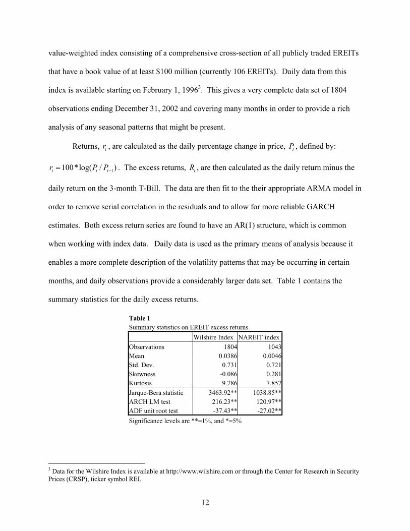
Returns, tr , are calculated as the daily percentage change in price, tP , defined by:
1100*log( / )t t tr P P−= . The excess returns, tR , are then calculated as the daily return minus the
daily return on the 3-month T-Bill. The data are then fit to the their appropriate ARMA model in
order to remove serial correlation in the residuals and to allow for more reliable GARCH
estimates. Both excess return series are found to have an AR(1) structure, which is common
when working with index data. Daily data is used as the primary means of analysis because it
enables a more complete description of the volatility patterns that may be occurring in certain
months, and daily observations provide a considerably larger data set. Table 1 contains the
summary statistics for the daily excess returns.
Table 1 Summary statistics on EREIT excess returns Wilshire Index NAREIT indexObservations 1804 1043Mean 0.0386 0.0046Std. Dev. 0.731 0.721Skewness -0.086 0.281Kurtosis 9.786 7.857Jarque-Bera statistic 3463.92** 1038.85**ARCH LM test 216.23** 120.97**ADF unit root test -37.43** -27.02**Significance levels are **=1%, and *=5%
3 Data for the Wilshire Index is available at http://www.wilshire.com or through the Center for Research in Security Prices (CRSP), ticker symbol REI.
13
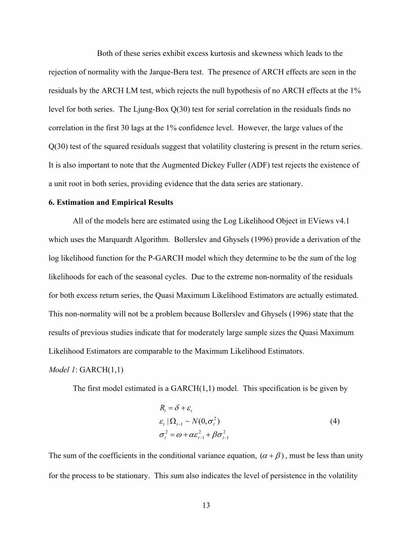
Both of these series exhibit excess kurtosis and skewness which leads to the
rejection of normality with the Jarque-Bera test. The presence of ARCH effects are seen in the
residuals by the ARCH LM test, which rejects the null hypothesis of no ARCH effects at the 1%
level for both series. The Ljung-Box Q(30) test for serial correlation in the residuals finds no
correlation in the first 30 lags at the 1% confidence level. However, the large values of the
Q(30) test of the squared residuals suggest that volatility clustering is present in the return series.
It is also important to note that the Augmented Dickey Fuller (ADF) test rejects the existence of
a unit root in both series, providing evidence that the data series are stationary.
6. Estimation and Empirical Results
All of the models here are estimated using the Log Likelihood Object in EViews v4.1
which uses the Marquardt Algorithm. Bollerslev and Ghysels (1996) provide a derivation of the
log likelihood function for the P-GARCH model which they determine to be the sum of the log
likelihoods for each of the seasonal cycles. Due to the extreme non-normality of the residuals
for both excess return series, the Quasi Maximum Likelihood Estimators are actually estimated.
This non-normality will not be a problem because Bollerslev and Ghysels (1996) state that the
results of previous studies indicate that for moderately large sample sizes the Quasi Maximum
Likelihood Estimators are comparable to the Maximum Likelihood Estimators.
Model 1: GARCH(1,1)
The first model estimated is a GARCH(1,1) model. This specification is be given by
21
2 2 21 1
| ~ (0, )t t
t t t
t t t
R
N
δ ε
ε σ
σ ω αε βσ−
− −
= +
Ω
= + +
(4)
The sum of the coefficients in the conditional variance equation, ( )α β+ , must be less than unity
for the process to be stationary. This sum also indicates the level of persistence in the volatility
14
shocks. A sum close to unity is favorable for providing evidence of a persistent volatility
process (Bollerslev 1986).
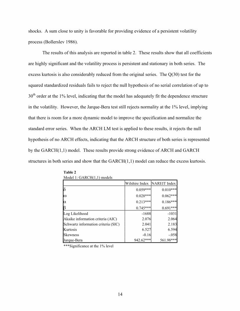
The results of this analysis are reported in table 2. These results show that all coefficients
are highly significant and the volatility process is persistent and stationary in both series. The
excess kurtosis is also considerably reduced from the original series. The Q(30) test for the
squared standardized residuals fails to reject the null hypothesis of no serial correlation of up to
30th order at the 1% level, indicating that the model has adequately fit the dependence structure
in the volatility. However, the Jarque-Bera test still rejects normality at the 1% level, implying
that there is room for a more dynamic model to improve the specification and normalize the
standard error series. When the ARCH LM test is applied to these results, it rejects the null
hypothesis of no ARCH effects, indicating that the ARCH structure of both series is represented
by the GARCH(1,1) model. These results provide strong evidence of ARCH and GARCH
structures in both series and show that the GARCH(1,1) model can reduce the excess kurtosis.
Table 2 Model 1: GARCH(1,1) models Wilshire Index NAREIT Index δ 0.059*** 0.010***ω 0.028*** 0.062***α 0.213*** 0.186***β 0.745*** 0.691***Log Likelihood -1688 -1031Akaike information criteria (AIC) 2.076 2.064Schwartz information criteria (SIC) 2.041 2.183Kurtosis 6.527 6.594Skewness -0.16 -.058Jarque-Bera 942.62*** 561.98******Significance at the 1% level
15
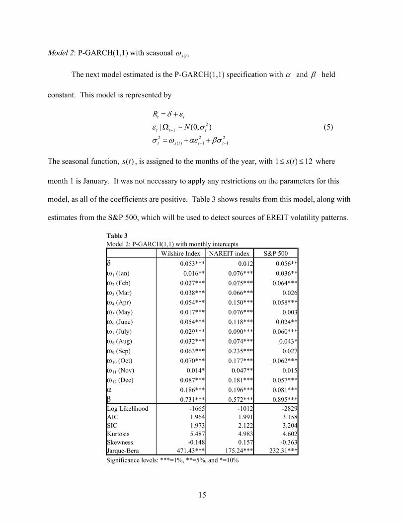
Model 2: P-GARCH(1,1) with seasonal ( )s tω
The next model estimated is the P-GARCH(1,1) specification with α and β held
constant. This model is represented by
21
2 2 2( ) 1 1
| ~ (0, )t t
t t t
t s t t t
R
N
δ ε
ε σ
σ ω αε βσ−
− −
= +
Ω
= + +
(5)
The seasonal function, ( )s t , is assigned to the months of the year, with 1 ( ) 12s t≤ ≤ where
month 1 is January. It was not necessary to apply any restrictions on the parameters for this
model, as all of the coefficients are positive. Table 3 shows results from this model, along with
estimates from the S&P 500, which will be used to detect sources of EREIT volatility patterns.
Table 3 Model 2: P-GARCH(1,1) with monthly intercepts Wilshire Index NAREIT index S&P 500 δ 0.053*** 0.012 0.056**ω1 (Jan) 0.016** 0.076*** 0.036**ω2 (Feb) 0.027*** 0.075*** 0.064***ω3 (Mar) 0.038*** 0.066*** 0.026ω4 (Apr) 0.054*** 0.150*** 0.058***ω5 (May) 0.017*** 0.076*** 0.003ω6 (June) 0.054*** 0.118*** 0.024**ω7 (July) 0.029*** 0.090*** 0.060***ω8 (Aug) 0.032*** 0.074*** 0.043*ω9 (Sep) 0.063*** 0.235*** 0.027ω10 (Oct) 0.070*** 0.177*** 0.062***ω11 (Nov) 0.014* 0.047** 0.015ω12 (Dec) 0.087*** 0.181*** 0.057***α 0.186*** 0.196*** 0.081***β 0.731*** 0.572*** 0.895***Log Likelihood -1665 -1012 -2829AIC 1.964 1.991 3.158SIC 1.973 2.122 3.204Kurtosis 5.487 4.983 4.602Skewness -0.148 0.157 -0.363Jarque-Bera 471.43*** 175.24*** 232.31***Significance levels: ***=1%, **=5%, and *=10%
16
This specification provides statistically significant estimates at the 1% level for nearly all
intercepts of both series. A noteworthy improvement of this model is the considerable decrease
in excess kurtosis and the Jarque-Bera test statistic of both index return series. For example, the
kurtosis of the Wilshire Index is reduced from 6.527 in the GARCH(1,1) model to 5.487 in this
model. Also, serial correlation is not found at up the 30th order in the squared residuals at the 1%
confidence level according to the Ljung-Box Q(30) test.
Both series display consistent patterns of markedly increased volatility in terms of the
seasonal intercept for the months of April, June, September, October and December. Note that
the Wilshire and the NAREIT series have similar volatility patterns in the parameter estimates,
but the magnitude of the parameters differ. The larger magnitude in the volatility of the
NAREIT index is most likely due to the shorter time period modeled. Several hypotheses can be
presented for the increase in volatility for these specific months. The past research on REITs
already presented shows their connection with variables from several markets, including the
stock, bond and real estate markets. It is possible that the seasonal volatility patterns of EREITs
are simply in line with the seasonal patterns of the overall stock market.
To test this hypothesis, the same P-GARCH model is applied to the excess returns of the
S&P 500 over the same sample period as the Wilshire Index (2/1/1996 – 12/31/2002). These
results can be seen in table 3. The S&P 500 presents similar increases in volatility for the
months of April, October and December, while other months such as February and August are
also both significant and higher. This suggests that some of the seasonal volatility of EREITs
can be attributed to the volatility fluctuations of the general stock market.
The commonly observed increased volatility in April and December is likely the effect of
year-end selling for tax purposes and then tax payment time in April. Glosten et al. (1993)

17
provide several explanations for why market volatility is higher in certain months. They
speculate that the fourth quarter, and December in particular, is an important holiday season for
consumer sales. Investors then begin to anticipate and predict the key consumer spending
figures, and this level of uncertainty about the state of the economy creates higher volatility
levels in the stock market. Glosten et al. notes that the higher volatility in October is due to the
inclusion of October 1987 in their sample period. However, this is not a valid explanation for
higher October volatility in this study because the sample period is from February 1996 forward.
As previous research has found EREITs to be correlated with interest rates, it is
appropriate to investigate possible seasonality in short-term interest rates that could affect EREIT
volatility patterns. Interest rate seasonality has been shown to be minor, if it exists at all. This is
not surprising because the implicit seasonal policy of the Federal Reserve has been to reduce,
and possibly eliminate, seasonal fluctuations in interest rates. Lawler (1979) found that the 3-
month T-Bill rates tend to be lower in February and then reach their peak from July to
September. Nonparametric tests of interest rate seasonality were performed by Sharp (1988), in
which he found evidence for seasonal variation in the short T-Bill rate from 1952-1985.
Indications that the short interest rate tended to be higher in July through September were also
found in this study. However, Barth and Bennett (1975) found no evidence for a systematic
month-to-month pattern in interest rates. The presence of seasonal volatility in the short-term
nominal interest rate was found by Jaditz (2000). He used monthly intercepts in the variance
equation to determine that a small degree of seasonal volatility is present in nominal interest
rates, with February being the most volatile month and December being the most stable. These
studies provide evidence for possible seasonality in both the mean and variance of short-term
interest rates. However, the overall volatility levels of short T-Bills are very small compared to
18
EREITs and other equities, and the variation from month to month in short T-Bill volatility
appears to be small, if it does indeed exist, and most likely is not a significant factor in the
seasonal fluctuations of EREIT volatility.
These results suggest that some of the seasonality of EREITs may be a result of the
underlying market volatility, but they also provide evidence that EREITs show signs of a unique
and more pronounced volatility pattern. The seasonality in EREITs is very well defined in terms
of the statistical significance of the ( )s tω parameters while the S&P 500 displays a less
pronounced pattern, as evidenced by the fewer number of significant intercept terms. The more
definite pattern visible in EREITs could be due to their correlation with the real estate market.
For example, the volatility increase of EREITs in June might be in response to the start of
increased activity in real estate as the summer months begin, as shown by Chinloy (1999). Also,
the lower levels of volatility seen in the winter months of January, February and March could be
the result of the decreased winter activity in real estate construction and home sales. This model
is a major improvement over the standard GARCH(1,1) model, but the P-GARCH process is still
being partially restricted by imposing the condition of ( )s tα α≡ . In the next model, this
condition will be eliminated and a more dynamic volatility process will be estimated.
Model 3: P-GARCH(1,1) with seasonal ( )s tω and ( )s tα
By allowing the autoregressive parameter, ( )s tα , to vary, a more flexible and realistic
model is formed. This P-GARCH model is given by
21
2 2 2( ) ( ) 1 1
| ~ (0, )t t
t t t
t s t s t t t
R
N
δ ε
ε σ
σ ω α ε βσ−
− −
= +
Ω
= + +
(6)

19
When this model is estimated with no restrictions placed on the coefficients, the Wilshire Index
model converges and produces positive variance estimates. However, several of the intercept
coefficients for the NAREIT index were negative, resulting in the possibility of an unrealistic
negative variance. To correct for this problem, the absolute value of the coefficients are
estimated, leading to positive values for all significant coefficients (Bester 1999). This
procedure is not fully theoretically justified but the results will still be presented here. Monte
Carlo tests were run on simulated data to ensure the usefulness of estimating the absolute value
of the coefficients. The results from these simulations show that, in general, the models
converge and tend to produce reliable estimates for some of the coefficients, but there is a
tendency for many of the coefficients of a 12 period model, such as the one used here, to not be
statistically different from zero. For example, 15 of the 25 parameter simulation estimates were,
on average, not statistically different from 0 at the 5% confidence level. A detailed summary of
the results and Monte Carlo procedures from these simulation tests are available in the appendix
in tables 5 and 6.
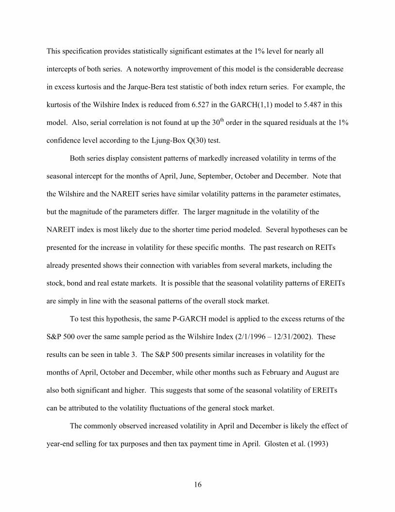
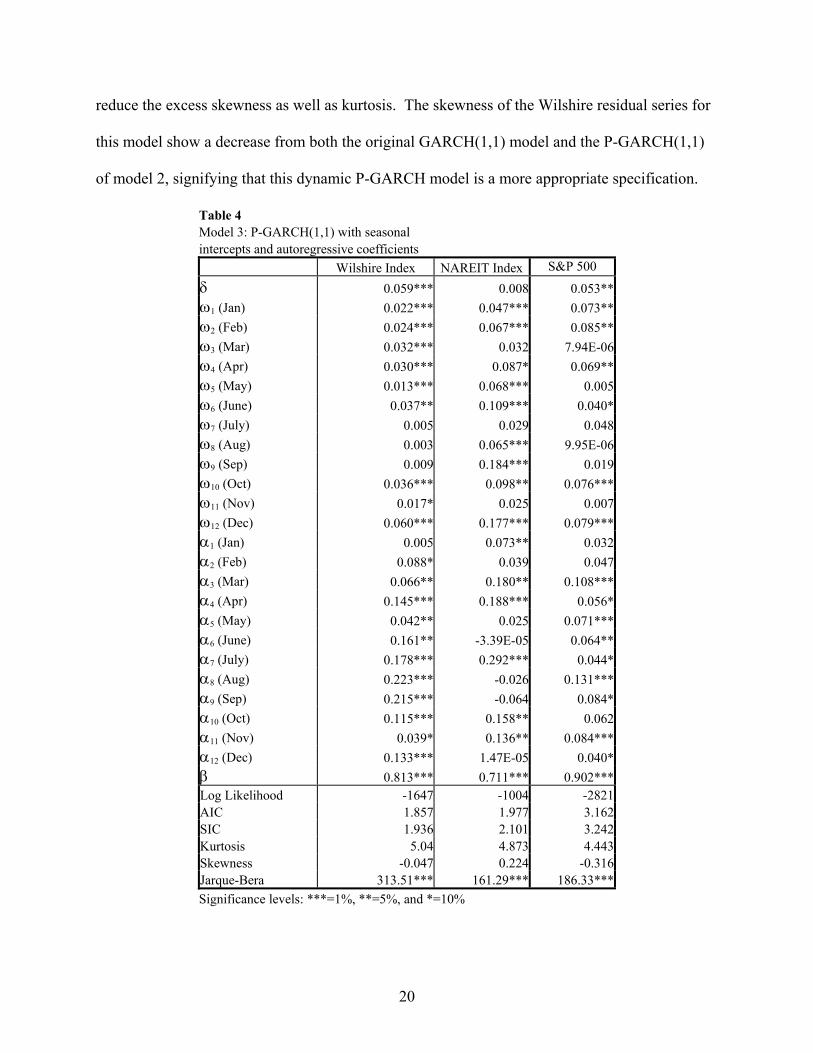
The results from the model 3 P-GARCH(1,1) estimation can be seen below in table 4.
Nearly all of the coefficients for the Wilshire Index are statistically significant at the 1% and 5%
levels. However the NAREIT Index parameters, specifically the ( )s tα parameters, are not as
consistent in their significance. This could be due to the different estimation technique used, or
the relatively smaller sample size of the NAREIT index which prevents this dynamic P-GARCH
process from being evident. There is no evidence of serial correlation in the first 30 lags of the
squared residuals at the 1% level by the Q(30) test. This model is able to further reduce the
excess kurtosis in both models, even though the null hypothesis of normality is still rejected.
Glosten et al. (1993) note that properly specified GARCH family models should be able to
20
reduce the excess skewness as well as kurtosis. The skewness of the Wilshire residual series for
this model show a decrease from both the original GARCH(1,1) model and the P-GARCH(1,1)
of model 2, signifying that this dynamic P-GARCH model is a more appropriate specification.
Table 4 Model 3: P-GARCH(1,1) with seasonal intercepts and autoregressive coefficients Wilshire Index NAREIT Index S&P 500
δ 0.059*** 0.008 0.053**ω1 (Jan) 0.022*** 0.047*** 0.073**ω2 (Feb) 0.024*** 0.067*** 0.085**ω3 (Mar) 0.032*** 0.032 7.94E-06ω4 (Apr) 0.030*** 0.087* 0.069**ω5 (May) 0.013*** 0.068*** 0.005ω6 (June) 0.037** 0.109*** 0.040*ω7 (July) 0.005 0.029 0.048ω8 (Aug) 0.003 0.065*** 9.95E-06ω9 (Sep) 0.009 0.184*** 0.019ω10 (Oct) 0.036*** 0.098** 0.076***ω11 (Nov) 0.017* 0.025 0.007ω12 (Dec) 0.060*** 0.177*** 0.079***α1 (Jan) 0.005 0.073** 0.032α2 (Feb) 0.088* 0.039 0.047α3 (Mar) 0.066** 0.180** 0.108***α4 (Apr) 0.145*** 0.188*** 0.056*α5 (May) 0.042** 0.025 0.071***α6 (June) 0.161** -3.39E-05 0.064**α7 (July) 0.178*** 0.292*** 0.044*α8 (Aug) 0.223*** -0.026 0.131***α9 (Sep) 0.215*** -0.064 0.084*α10 (Oct) 0.115*** 0.158** 0.062α11 (Nov) 0.039* 0.136** 0.084***α12 (Dec) 0.133*** 1.47E-05 0.040*β 0.813*** 0.711*** 0.902***Log Likelihood -1647 -1004 -2821AIC 1.857 1.977 3.162SIC 1.936 2.101 3.242Kurtosis 5.04 4.873 4.443Skewness -0.047 0.224 -0.316Jarque-Bera 313.51*** 161.29*** 186.33***Significance levels: ***=1%, **=5%, and *=10%
21
The estimates of β for both series are different than in the simple P-GARCH model,
indicating that allowing for the seasonal impact of news arrival changes the smooth evolution of
the volatility, in an ideal model β would remain relatively stable. For two months of the
Wilshire Index estimates, the sum of ( )s tα β+ exceeds unity, however this does not mean that
the process is not covariance stationary. For a P-GARCH(1,1) model the condition that
( )( ) 1s tα β+ < for all ( )s tα is a sufficient but not necessary condition for the process to be
stationary. Bollerslev and Ghysels (1996) show that a P-GARCH(1,1) model is stationary if the
geometric mean of all the ( )s tα β+ terms is less than unity4. The geometric mean of these terms
in the Wilshire estimates is 0.928 so the process is indeed covariance stationary. It should be
noted that both the Akaike Information Criteria (AIC) and the Schwartz Information Criteria
(SIC) of the Wilshire Index appear to slightly favor this new model over both models 1 and 2,
suggesting the importance for a less restrictive model of the periodic structure of EREIT
volatility. The AIC and SIC are model selection criteria similar to an adjusted 2R , but they both
place a larger penalty on the loss of degrees of freedom that occurs when a model is expanded.
For the AIC and SIC, a smaller number is associated with a better model. The SIC shows a
smaller improvement than the AIC; this could be a result of expanding the model because the
definition of the SIC favors simpler models5.
A closer look at the results of this model shows the same seasonal patterns in the ( )s tω
parameter as model 2 and also reveals a new pattern for the autoregressive parameter, ( )s tα . A
majority of the following analysis will be limited to the Wilshire Index results, as they are more
4 The geometric mean of the sequence 12
( ) ( ) 1s t s tα β
=+ is defined by
112 12
( )( ) 1
( )s ts t
α β=
+
∏
5 For a more detailed description of AIC and SIC see Greene (2003) pp. 159-160.
22
reliable and no restrictions are needed for the process to be well defined, and the NAREIT index
was originally included only as means for comparison. The autoregressive coefficients are
consistently larger for the summer months of June, July, August and into September. This
indicates that EREITs have a greater sensitivity to news arrival during the summer.
Once again, a similar model was estimated for the S&P 500 in order to investigate the
source of the seasonal patterns of EREITs. The findings of the S&P 500 model are similar to
those from model 2 and the results can be seen in table 4. The S&P 500 has slightly larger
autoregressive coefficients in the summer months, specifically August and September. However,
the seasonality in the ( )s tα parameter is not as pronounced and consistently different from zero as
in the Wilshire Index, indicating other seasonal factors at work in EREIT returns. Aside from
the effects of the general stock market, the values of ( )s tα may be higher in the Wilshire Index as
a result of EREITs interaction with the real estate market. The increased activity of the real
estate market in the summer months would make it more sensitive to any news arrival that could
potentially help or hurt this crucial real estate season. This increased news sensitivity in the real
estate market could cause the direct impact of news arrival relating to real estate to have a larger
impact on EREIT volatility, thereby increasing ( )s tα for these months.
To ensure the reliability of using Log Likelihood estimation in Eviews as the estimation
technique for P-GARCH(1,1) models, Monte Carlo simulations were run on simulated data using
the same P-GARCH models and procedures as used in models 2 and 3. All of the Monte Carlo
simulations were performed using a sample size of 1800, which is comparable to the sample size
of the Wilshire Index. However, 3600 observations were actually simulated and the first 1800
observations discarded to avoid start-up problems (Bollerslev and Ghysels 1996). The
appropriate P-GARCH(1,1) models with periodic cycles of lengths 6 and 12 were simulated and
23
then tested using the Log Likelihood estimation procedure in EViews. The simulation results
demonstrate that this method produces reliable coefficient estimates for model 2. The procedure
for the non-restricted model 3 was reliable for a cycle of length 6 but lost some of its accuracy
for 12 phases. However, 17 of the 25 parameters were still estimated to be, on average,
statistically different from 0 at the 5% confidence level, and these coefficients were also
relatively close to their true value. These results provide evidence for the validity of the Log
Likelihood estimation procedure for these P-GARCH(1,1) models. The exact simulation results
have been included in the Appendix in tables 7-9.
7. Conclusion
The estimation of these three models illustrates the presence of a P-GARCH structure
which allows for greater flexibility in modeling the seasonal volatility patterns of EREITs.
Model 1 shows that a GARCH(1,1) specification is an appropriate model to explain the volatility
structure, but does not address the issue of seasonality. Using model 1 as a benchmark, the two
P-GARCH models provide a richer dynamic description of the periodic volatility in EREIT
returns. Importantly, not only are most of the parameters for all the models significant and
positive, but also each model reduces the amount of excess kurtosis, thereby bringing the
residual series closer to normality. It should also be noted that all models estimated, expect the
NAREIT index in model 3, are found to fit the P-GARCH specification and have positive
variance without the need for parameter restrictions.
In summary, the study finds that EREITs display seasonal volatility patterns in which
their overall return volatility is higher during the months of April, June, September, October, and
December. The hypotheses investigated here show that some of the EREIT seasonality may be
attributed to the volatility patterns of the primary stock markets that EREIT shares trade in, such
24
as the S&P 500. However, the seasonal volatility patterns of EREIT returns are more
pronounced and persistent than the seasonal patterns of the major stock markets, perhaps a result
of EREITs connection with the highly seasonal real estate market. The sensitivity of EREIT
returns to news arrival is found to be higher during the summer months, possibly as a result of
the importance of these months in the real estate market.
The problems encountered in estimating these models are not major but could be resolved
or improved in future research. The restrictions applied when estimating the NAREIT index
estimates in model 3 are not fully theoretically justified and could be eliminated with a more
advanced estimation technique, or possibly by analyzing a longer sample range. Also, the
inconsistency of the parameter estimates for the NAREIT Index in model 3 could potentially be
alleviated with a larger and higher quality data set.
Overall, the findings are promising for the application of P-GARCH models in
identifying seasonal volatility patterns of EREITs. The results also provide a more complete
description of EREIT volatility patterns that can be used as a framework for those involved in
trading EREITs or EREIT options. Potential directions for future research include the
development of more sophisticated P-GARCH models and a more in-depth interpretation and
explanation of the seasonal volatility patterns of EREITs.
25
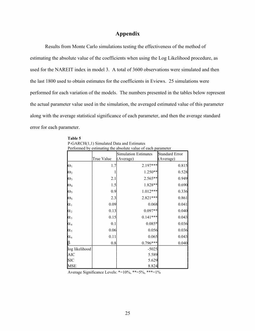
Appendix
Results from Monte Carlo simulations testing the effectiveness of the method of
estimating the absolute value of the coefficients when using the Log Likelihood procedure, as
used for the NAREIT index in model 3. A total of 3600 observations were simulated and then
the last 1800 used to obtain estimates for the coefficients in Eviews. 25 simulations were
performed for each variation of the models. The numbers presented in the tables below represent
the actual parameter value used in the simulation, the averaged estimated value of this parameter
along with the average statistical significance of each parameter, and then the average standard
error for each parameter.
Table 5 P-GARCH(1,1) Simulated Data and Estimates Performed by estimating the absolute value of each parameter
True Value Simulation Estimates (Average)
Standard Error (Average)
ω1 1.7 2.197*** 0.815ω2 1 1.250** 0.528ω3 2.1 2.565** 0.949ω4 1.5 1.828** 0.690ω5 0.9 1.012*** 0.336ω6 2.3 2.821*** 0.861α1 0.09 0.068 0.041α2 0.13 0.097** 0.040α3 0.15 0.141*** 0.043α4 0.1 0.085* 0.036α5 0.06 0.056 0.036α6 0.11 0.065 0.043β 0.8 0.796*** 0.040log likelihood -5025 AIC 5.589 SIC 5.629 MSE 8.824 Average Significance Levels: *=10%, **=5%, ***=1%

26
Table 6 P-GARCH(1,1) Simulated Data and Estimates Performed by estimating the absolute value of each parameter
True Value Simulation Estimates (Average)
Standard Error (Average)
ω1 1.7 2.530* 1.346ω2 1 1.372 0.890ω3 2.1 2.244* 1.175ω4 1.5 1.93** 1.040ω5 0.9 1.074 0.496ω6 2.3 2.821** 1.080ω7 2 2.312* 1.224ω8 1.8 2.355** 1.193ω9 1 1.467 0.907ω10 1.3 1.703** 0.715ω11 2.2 2.991* 1.231ω12 2.5 3.485* 1.787α1 0.09 0.062 0.052α2 0.13 0.11* 0.062α3 0.15 0.144** 0.063α4 0.1 0.089** 0.055α5 0.06 0.039 0.050α6 0.11 0.089** 0.068α7 0.09 0.076 0.060α8 0.14 0.108 0.057α9 0.12 0.105** 0.057α10 0.09 0.064 0.053α11 0.13 0.088 0.059α12 0.16 0.134** 0.055β 0.8 0.794*** 0.040log likelihood -5166 AIC 5.763 SIC 5.839 MSE 21.940 Average Significance Levels: *=10%, **=5%, ***=1%
27
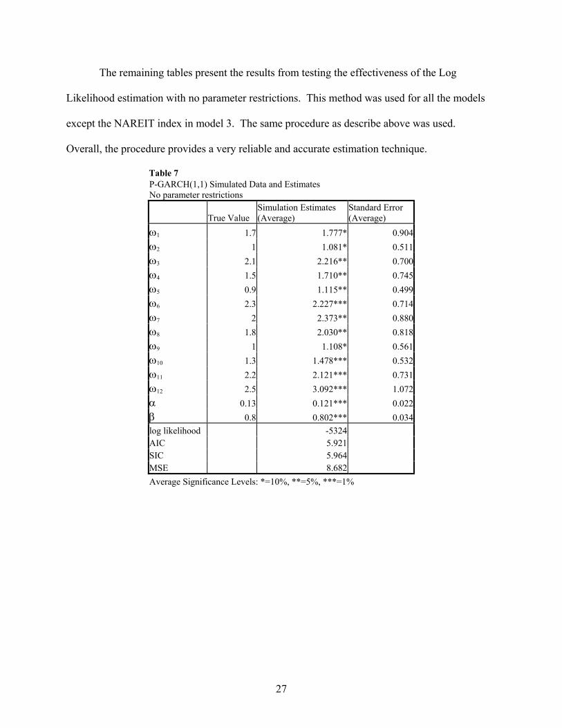
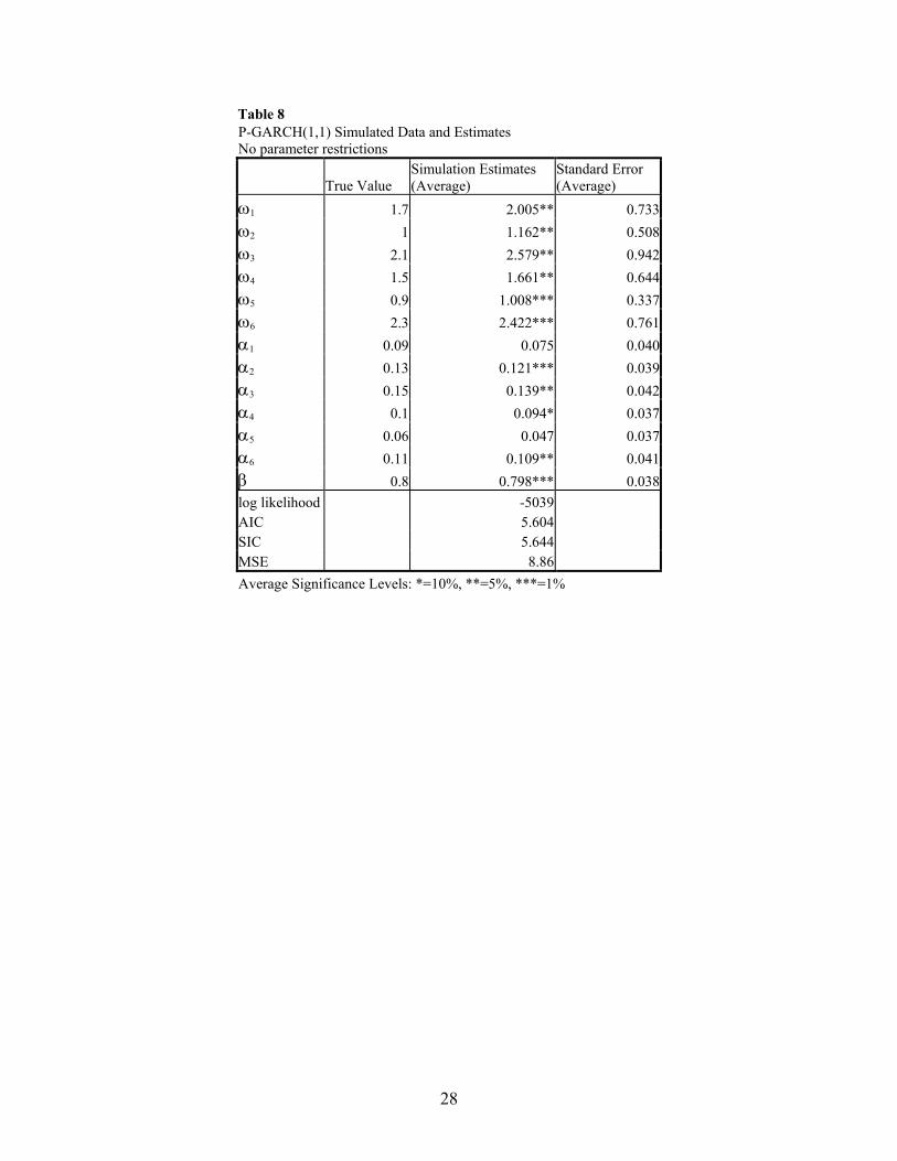
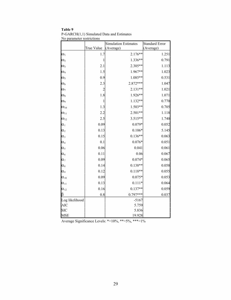
The remaining tables present the results from testing the effectiveness of the Log
Likelihood estimation with no parameter restrictions. This method was used for all the models
except the NAREIT index in model 3. The same procedure as describe above was used.
Overall, the procedure provides a very reliable and accurate estimation technique.
Table 7 P-GARCH(1,1) Simulated Data and Estimates No parameter restrictions
True Value Simulation Estimates (Average)
Standard Error (Average)
ω1 1.7 1.777* 0.904ω2 1 1.081* 0.511ω3 2.1 2.216** 0.700ω4 1.5 1.710** 0.745ω5 0.9 1.115** 0.499ω6 2.3 2.227*** 0.714ω7 2 2.373** 0.880ω8 1.8 2.030** 0.818ω9 1 1.108* 0.561ω10 1.3 1.478*** 0.532ω11 2.2 2.121*** 0.731ω12 2.5 3.092*** 1.072α 0.13 0.121*** 0.022β 0.8 0.802*** 0.034log likelihood -5324 AIC 5.921 SIC 5.964 MSE 8.682 Average Significance Levels: *=10%, **=5%, ***=1%
28
Table 8 P-GARCH(1,1) Simulated Data and Estimates No parameter restrictions
True Value Simulation Estimates (Average)
Standard Error (Average)
ω1 1.7 2.005** 0.733ω2 1 1.162** 0.508ω3 2.1 2.579** 0.942ω4 1.5 1.661** 0.644ω5 0.9 1.008*** 0.337ω6 2.3 2.422*** 0.761α1 0.09 0.075 0.040α2 0.13 0.121*** 0.039α3 0.15 0.139** 0.042α4 0.1 0.094* 0.037α5 0.06 0.047 0.037α6 0.11 0.109** 0.041β 0.8 0.798*** 0.038log likelihood -5039 AIC 5.604 SIC 5.644 MSE 8.86 Average Significance Levels: *=10%, **=5%, ***=1%
29
Table 9 P-GARCH(1,1) Simulated Data and Estimates No parameter restrictions
True Value Simulation Estimates (Average)
Standard Error (Average)
ω1 1.7 2.176** 1.251ω2 1 1.336** 0.791ω3 2.1 2.305** 1.113ω4 1.5 1.967** 1.023ω5 0.9 1.085** 0.531ω6 2.3 2.872*** 1.047ω7 2 2.131** 1.021ω8 1.8 1.926** 1.071ω9 1 1.132** 0.770ω10 1.3 1.503** 0.705ω11 2.2 2.501** 1.118ω12 2.5 3.515** 1.740α1 0.09 0.079* 0.052α2 0.13 0.106* 5.145α3 0.15 0.136** 0.063α4 0.1 0.076* 0.051α5 0.06 0.041 0.061α6 0.11 0.06 0.067α7 0.09 0.074* 0.065α8 0.14 0.138** 0.058α9 0.12 0.118** 0.055α10 0.09 0.075* 0.053α11 0.13 0.111* 0.064α12 0.16 0.137** 0.059β 0.8 0.797*** 0.037Log likelihood -5167 AIC 5.759 SIC 5.836 MSE 19.928 Average Significance Levels: *=10%, **=5%, ***=1%
30
References
Barth, James R., and Bennett, James T. (1975), “Seasonal Variation in Interest Rates,” The Review of Economics and Statistics, 57, 80-83.
Beller, Kenneth, and Nofsinger, John R. (1998), “On Stock Return Seasonality and Conditional
Heteroskedasticity,” The Journal of Financial Research, 21:2, 229-246. Bester, Alan. (1999), “Seasonal Patterns In Futures Market Volatility: A P-GARCH Approach,”
Duke Journal of Economics, 11, 65-102. Bollerslev, T. (1986), “Generalized Autoregressive Conditional Heteroskedasticity,” Journal of
Econometrics, 31, 307-327. Bollerslev, T.R. (1987), “A Conditionally Heteroskedastic Time Series Model For Speculative
Prices and Rates of Return,” Review of Economics and Statistics, 69, 542-547. Bollerslev, T.R., Chou, Y., and Kroner, K.F. (1992), “ARCH Modeling in Finance: A Review of
the Theory and Empirical Evidence,” Journal of Econometrics, 52, 5-59. Bollerslev, T.R., Engle, R.F., and Wooldridge, J.M. (1988), “A Capital Asset Pricing Model with
Time Varying Covariances,” Journal of Political Economy, 96, 116-131. Bollerslev, T., and Ghysels, E. (1996), “Periodic Autoregressive Conditional
Heteroskedasticity,” Journal of Business and Economic Statistics, 14:2, 139-151. Chan, K.C., Hendershott, Patric H., and Sanders, Anthony B. (1990), “Risk and Return on Real
Estate: Evidence from Equity REITs,” AREUEA Journal, 18:4, 431-452. Chinloy, Peter. (1999), “Housing, Illiquidity, and Wealth,” Journal of Real Estate Finance and
Economics, 19:1, 69-83. Devaney, Michael (2001), “Time Varying Risk Premia for Real Estate Investment Trusts: A
GARCH-M model,” The Quarterly Review of Economics and Finance, 41, 335-346. Elyasiani, Elyas, and Mansur, Iqbal (1998), “Sensitivity of the Bank Stock Returns Distributions
to Changes in the Level and Volatility of Interest Rate: A GARCH-M model,” Journal of Banking and Finance, 22, 535-563.
Engle, R.F. (1982), “Autoregressive Conditional Heteroskedasticity With Estimates of the
Variance of U.K. Inflation,” Econometrica 50, 987-1008. Engle, R.F., Ito, T., and Lin, W.L. (1990), “Meteor Showers or Heat Waves? Heteroskedastic
Intra-daily Volatility in the Foreign Exchange Market,” Econometrica, 58, 525-542.
31
Fama, E.F., and French, K.R. (1993), “Common Risk Factors in the Returns on Stock and Bonds,” Journal of Financial Economics, 33, 3-56.
Friday, Swint H., and Peterson, David R. (1997), “January Return Seasonality in Real Estate
Investment Trusts: Information vs. Tax-Loss Selling Effects,” The Journal of Financial Research, 20:1, 33-51.
Glosten, Lawrence R., Jaganathan, Ravi, and Runkle, David E. (1993), “On the Relationship
Between the Expected Value and the Volatility of the Nominal Excess Return on Stocks,” The Journal of Finance, 48:5, 1779-1801.
Graff, Richard A. (1998), “The Impact of Seasonality on Investment Statistics Derived from
Quarterly Returns,” Journal of Real Estate Portfolio Management, 4:1, 1-16. Greene, William H. (2003). Economic Analysis, 5th ed., Upper Saddle River, NJ: Pearson
Education Inc. Gyourko, Joseph, and Keim, Donald B. (1992), “What does the Stock Market Tell us About Real
Estate Returns,” AREUEA Journal, 20:3, 457-486. Hamilton, James D. (1994), Time Series Analysis. Princeton, NJ: Princeton University Press. Hamilton, James D., and Lin, Gang (1996), “Stock Market Volatility and the Business Cycle,”
Journal of Applied Econometrics, 11:5, 573-593 Jaditz, Ted. (2000), “Seasonality in Variance is Common in Macro Time Series,” Journal of
Business, 73:2, 245-254. Lamoureus, C.G., and Lastrapes, W.D. (1990), “Heteroskedasticity in Stock Return Data:
Volume Versus GARCH effects,” Journal of Finance, 45, 221-229. Lawler, Thomas A. (1979), “Federal Reserve Strategy and Interest Rate Seasonality: Note,”
Journal of Money, Credit and Banking, 11:4, 494-499. Nelson, D.B., and Cao, C.Q. (1992), “Inequality Constraints in the Univariate GARCH Model,”
Journal of Business and Economic Statistics, 10, 229-235. Peterson, James D., and Hsieh, Cheng-Ho. (1997), “Do Common Risk Factors in the Returns on
Stock and Bonds Explain Returns on REITs?” Real Estate Economics, 25:2, 321-345. Sharp, Keith P. (1988), “Tests of U.S. Short and Long Interest Rate Seasonality,” The Review of
Economics and Statistics, 70:1, 177-182. Young, Michael S., Geltner, David M., McIntosh, Willard, and Poutasse, Douglas M. (1996),
“Understanding Equity Real Estate Performance: Insights from the NCREIF Property Index,” Real Estate Review, 25:4, 4-16.