Real and financial crises in the Keynes-Kalecki structuralist model: Anagent-based approach

Bill Gibson†and Mark Setterfield††1

Abstract

Agent-based models are inherently microstructures–with their attention to agent behavior in a field context–and only aggregate up to systems with recognizable macroeconomic characteristics. One might ask whythe traditional Keynes-Kalecki or structuralist (KKS) model would bear any relationship to the multi-agentmodeling approach. This paper shows how KKS models might benefit from agent-based microfoundations,without sacrificing traditional macroeconomic themes, such as aggregate demand, animal spirits and en-dogenous money. Above all, the integration of the two approaches gives rise to the possibility that a KKSsystem–stable over many consecutive time periods–might lurch into an uncontrollable downturn, from whicha recovery would require outside intervention. As a by-product of the integration of these two popularapproaches, there emerges a cogent analysis of the network structure necessary to bind real and financialagents into a integrated whole. It is seen, contrary to much of the existing literature, that a highly connectedfinancial system does not necessarily lead to more crashes of the integrated system.

Keywords: systemic risk; crash; herding; Bayesian learning; endogenous money; preferential attachment;agent-based models.JEL codes: D58, E37, G01, G12, B16, C00.

1. Introduction

At first glance, Keynes-Kalecki or structuralist (KKS) macroeconomics and agent-based models wouldseem to be strange bed-fellows. Structuralists since Taylor [28] have integrated the financial and real sidesof the models but mostly through the interest rate [27] and the profit rate [29]. Since then the literatureon “financialization” has emphasized the bloat, waste, and inequality ushered in by growth of the financialservices sector [7, 21]. This literature has been less concerned with the central role played by finance inchanneling savings into investment. Early Keynesians were certainly concerned and it was immediatelyrecognized by Robertson [22] and later by Chick [6] that at the core of the Keynesian economy was awell-functioning financial system capable of creating money.2 The system transfers purchasing power fromthose who wish to invest less than they save to their counterparts, those who want to invest more. Anyinterruption in this flow of funds spreads through the rest of the economy through the multiplier-acceleratorprocess, creating havoc.

1Version 3.6. †John Converse Professor of Economics, University of Vermont, Burlington, VT 05405; e-mailbill.gibson@uvm.edu; data for replication at http://www.uvm.edu/∼wgibson.††New School for Social Research and MaloneyFamily Distinguished Professor of Economics, Trinity College, Hartford, CT 06106; e-mail mark.setterfield@newschool.edu.Thanks to Amitava Dutt, Jerry Epstein, Diane Flaherty, Arjun Jayadev, Blake LeBaron, Victor Lesser, Suresh Naidu, AndreNeveu, Rajiv Sethi, Gil Skillman, Peter Skott, Daniel Thiel and Roberto Veneziani for useful comments on earlier versions.Jonas Oppenheim provided an invaluable critical reading of the final draft. Programming assistance by Paul Wright is alsogratefully acknowledged. We wish to thank Jeannette Wicks-Lim for making available advanced computational facilities of thePolitical Economy Research Institute at UMass, Amherst. Finally, three anonymous reviewers of the journal made valuablecomments that contributed significantly to the paper.

2See also Gibson and Setterfield [12].

Preprint submitted to Metroeconomica. 2018;00:1–27. https://doi.org/10.1111/meca.12201 May 15, 2018

Constructing convincing models of real-financial interaction, however, has been made difficult by theinherent complexity and interlinked nature of the financial system. Recent advances in agent-based modelingwith its focus on concentration and contagion across structured networks offer an opportunity for relativelydeep integration with KKS models. This paper shows how such integration might be accomplished and howthe central features of both approaches can be preserved in the merging of the two schools of thought.

Benefits accrue to both sides: structuralists have traditionally waved off the criticism that the micro-foundations of their models are weak and not explicitly tied to standard optimization models [25]. Mi-crofoundations in multi-agent models, however, are not always based on strict rationality. Agents are, bydefinition, boundedly rational; they are heterogeneous, sometimes myopic and generally incapable of makingrigorous inter-temporal trade-offs. Random elements play an important role, as does asymmetric infor-mation, incomplete contracts and other institutional constraints. These are all features that structuralistscommonly include in their macro models, but by assumption, rather than their having been derived fromsome microfoundation. On the other hand, the benefit to standard agent-based models is the integration ofthe real side into an explicitly financial model. This has been ably attended to in the past, of course, butthe Keynesian quantity adjustment process, with its emphasis on aggregate demand, is less visible in theexisting literature [1, 9]. Moreover, tracing the flows from surplus firms, those that invests less than theysave, to deficit firms, those that do the opposite, is not as easily seen in the standard literature as in themodel to follow. This perspective shows explicitly the conditions under which money must be endogenouslycreated and, moreover, allows for animal spirits to be an explicit driver of the level of economic activity.Prominent and popular financial models, such as Gai et al. [10], focus on contagion in the interbank market.The framework presented here is more concerned with the Keynesian features of modern capitalism, mostspecifically that an independent investment function drives the level of savings instead of the reverse as wellas the irrepressibility of endogenous money.

Setterfield and Budd [24] make a first step toward integrating the KKS perspective with agent-basedmodels. In that model, each agent is essentially its own KKS economy, with its own aggregate demand andsavings-investment balance. Agent interaction is limited to a “blackboard” communication system, in whichan agent’s incentive to invest is affected by the performance of its colleagues. Aggregate demand is notshared among firm agents, however, nor is there any explicit modeling of the financial sector.

Beginning with a multi-agent KKS model, this paper integrates a financial sector, inspired by the agent-based literature [16, 26, 14, 30, 19, 31, and many others]. The result is a model of the economy with twoagent sets, real sector firms and financial sector intermediaries. It is seen that financial intermediation canconstrain investment spending by firms, and hence the pace of growth in the real sector. Meanwhile, theprofits and savings generated in the real sector affect the ability and willingness of financial intermediariesto lend. The microfoundations are based on Bayesian learning [5] in which a prior public signal is updatedby way of a private signal based on the performance of the firms to which the financial agent is linked.

The paper is organized as follows. The next section outlines the design concepts and coordinationenvironment of the two agent sets. Section 3 discusses the main results of the model, endogenous moneyand the possibility of a real-financial crisis. It is seen that the integration of the two approaches allows animportant role for network structure, whether financial agents are linked randomly or by way of preferentialattachment. The fourth section concludes. An appendix contains the pseudo code of the model.3.

2. Design concepts

One way to initiate the transition from the pure KKS to a framework that integrates the multi-agentapproach is to individually model workers and capitalists and the full range of economic decisions theymake. This approach could be extended to the government, the financial sector and the central bank. A

3 Replication code is here. The model can be run using only the NetLogo software but was run for the purposes of this paperin “headless” configuration on the Vermont Advanced Computer Core Cluster at the University of Vermont. Supplementalmaterial for sensitivity analysis is here.

2

fully granular model would show all the inner-workings of the economy in exquisite detail and one would hopeand expect that the agent model would fully align with all the main features of the structuralist macromodel.

In a closed economy with no public sector, however, the structuralist model often invokes the assumptionthat workers do not save and capitalist save out of profits. This confers a significant degree of simplificationsince Walras’ law, which implies that the sum of agent savings is equal investment, the need to modelworkers’ behavior directly. In general, there would be no reason to make the assumption that workers do notsave in an agent-based model. Here, however, the project is to link the structuralist macro and agent-basedmethods and so the same assumption is maintained. Workers are still present in the agent model, but onlyimplicitly, as measured by the strength of their bargaining power on firm profitability and thus firm savings.

This simplification also enables the model to account for the interaction of just two kinds of agents: firmsand financial, without the complexity of a full agent-based system that might obscure the comparison ofthe two methods. Moreover, structuralist models can already adequately handle the kind complexity thatarises from the interaction of workers and capitalists. Attention here is paid to another level in which thestructuralist model is less competent and well worked out, that of the relationship between firms and theirfinancial agents.

In an economy with a single firm, the savings generated by that firm must be equal to total investment.When there are heterogeneous firms, some generate financial surpluses when they save more than they investand financial deficits when the opposite is true. The primary role of the financial system is intermediation,facilitating the flow of funds from surplus to deficit firms.

In the model of this paper, there are two agent sets: firms, which undertake all savings and investment,and financial agents that provide intermediation services. Financial agents neither save nor invest. Simplebehavioral rules are defined for these two agent classes and the macro performance of the model arises asan emergent property of their interaction. There is no policy authority or explicit monetary policy and alladaptation is through Bayesian and reinforcement learning.

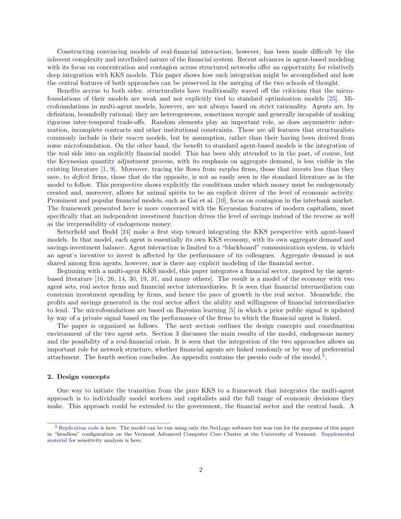
Figure 1 illustrates the three principal structural features of the multi-agent model, firms, financialagents, and financial network architecture. Each firm, represented as a square, operates only one productionprocess, combining capital and labor to satisfy demand for a homogeneous good.4 The key decision for firmsis whether and how much to invest. Investment is based on expectations about future market conditions andfirms’ ability to cover any short-fall in savings, relative to planned investment, through borrowing from otherfirms with the help of one or more financial agents. At each sweep of the model, surplus firms, shown asdark squares, make deposits with their resident financial agents, represented by numbered circles. Financialagents must then decide whether to grant loan requests to deficit firms, shown as light squares. The decisionof financial agents is also binary: lend/do not lend. This decision depends on their forecasts of the probabilitythat the loan will be paid back, dark for “bullish” and light for “bearish”.

Each financial agent can at most offer direct financing for one production process, the one with whichit is permanently associated. That same agent can, however, be called upon to provide indirect financingto another firm by way of a financial agent to which it is linked. Thus a bullish financial agent that lackssufficient liquidity to meet the demand for loans from its associated firm, may arrange for a loan from oneof its linked neighbors.

That financial firms only borrow from their linked neighbors is the “one-ply” assumption and is the pointat which network analysis–agents dispersed on grid–adds to the standard conceptual framework of the KKSmodel. Indeed without the one-ply assumption, firms could chain across the entire grid, borrowing for allavailable sources of savings, directly or indirectly. No financial system frictions could arise to interrupt thegrowth of the system and the model would effectively revert to the standard KKS model, in which there isalways finance available for any desired investment.5

4This is the easiest way to think about the adjustment mechanisms in the model. Equivalently, there could be heterogeneousgoods with prices adjusting behind the scenes. Price movements would shift investible surplus from one firm to another, butthe overall macro properties of the model would remain unchanged.

5The reader could reasonably wonder whether a two-ply assumption might be more realistic, coming closer to the way inwhich financial firms are linked in the real world. On reflection, however, it is apparent that the crucial distinction is between alimited ply and full grid access. Multi-ply systems can always be converted to one-ply systems, by eliminating the middleman,

3

(3) Heterogeneous forecasts (4) Emerging grid spanning cluster

(2) Period 1(1) Period 0

0"

2"

1"

3"

4"

0"

2"

1"

3"

4"

0"

2"

1"

3"

4"

0"

2"

1"

3"

4"

Figure 1: Structural features of the multi-agent model

The linked neighbor may have refused a loan to its own (deficit) firm on the grounds of a bearish forecast.It is nonetheless willing to accept the indirect request of its neighbor. This feature of the model is designedto capture the “originate and distribute” characteristic of the financial system. Indirect loans are viewed asless risky since deficit firms are vetted by their own financial agent and indirect financing is, therefore, neverrefused. Figure 1 shows, however, that firms can have direct access to more than one financial agent. It mayseem from figure 1 that there are more financial agents than firms, inverting reality. Note, however, thatfinancial agents are not conterminous with financial firms, an association of financial agents, and that thenumber of financial firms is not defined within the model. In any case, the latter would already be includedin the agent set firms, which earn profits and pay wages. Consequently, there is no explicit interest rate sinceprices are not explicit due to the assumption of a single homogeneous good.

To capture the locality of intermediation, information constraints and boundedness on the rationalityof the financial agents, however, indirect borrowing must be limited to some degree. This is achieved byimposing a restriction on the connectedness of the system through the number of plys to which each financialagent has indirect access. A simple but useful assumption is to limit the number of plys to one. This providesa clear distinction between KKS systems in which the supply of credit constrains real activity and those in

which has been done here for simplicity.

4

which it does not.If the number financial agents is less than the number of firms, large deficits of aggregate demand arise,

since so many deficit firms are unable to find financing for their projects. A far less restrictive assumption isthat the number of financial agents, m, is greater than then number of firms, n. This assumption producesreasonably robust growth and prevents subsets of firms from experiencing very low levels of effective demandand capacity utilization when the rest of the grid is booming. The two critical assumptions of the model arethen one-ply and m > n and it should now be clear that the model would behave in highly unrealistic wayif either of these assumptions were relaxed.

Network architecture is represented by the edges joining the numbered financial agents in figure 1, andinfluences how financial surpluses are allocated.6 Suppose that the surplus firm, shown in dark gray in thefirst panel of figure 1, makes a deposit with financial agent 0 which is connected to financial agent 1 andthrough torus wrapping to financial agent 2. Financial agent 1 is bearish but in any case has nothing to do,since the firm to which it would lend is already in surplus. Financial agent 2, however, serves a deficit clientand is connected to financial agent 0, associated with a surplus firm. Agent 2 is also connected to 3, who isassociated with a deficit firm and has no liquidity. Financial agent 2 then calls on financial agent 0 to makethe surplus available for its client. Savings is thereby channeled from a surplus to a deficit firm.7

Agent 3 is bearish, but even had 3’s forecast been bullish, it might have been stymied in its effort toprovide indirect financing for its deficit firm. Whether 3 has indirect access to financial agent 0’s funds isa setting of the model and determines the degree of connectedness of the financial system. KKS modelsthat have no constraint on interbank borrowing essentially allow each financial agent complete access to allother financial agents on the grid. This is the assumption that implicitly underpins KKS models without afinancial sector, models in which money is endogenous.

Even under the one-ply restriction, money is still endogenous. To see this, first note that behavioraldecision rules in multi-agent systems are executed asynchronously. This asynchronicity allows the possibilityof collisions, that is, conflicting claims on financial resources. This works as follows: At the end of eachperiod, firms deposit their savings out of profits determined by a given savings propensity. At the beginningof the following period, financial agents respond to demand for this liquidity from both surplus and deficitfirms. If a deficit firm applies for a loan before the surplus firm has had a chance to invest its funds, acollision is created. The conflict can only be resolved by allowing financial agents to create money.8 Theendogeneity of the money supply is critical to the macro performance of the model, since if investment werealways constrained by savings, there would be no room for expectations-driven growth.

The second panel of figure 1 shows the same neighborhood one period later. Note that the networkarchitecture, the number of firms, and the number and location of financial agents remains fixed. Observethat the surplus firm of the first period is now in deficit and the formerly deficit firms in the north-east andsouth-east positions are now in surplus. This change occurs because aggregate demand alters the ability offirms to save and their incentive to invest. The forecasts of financial agents have also changed. Generally,forecasts remain heterogenous as shown in the third panel of figure 1. It is possible for a grid-spanningcluster of opinion to arise, however, as illustrated in the fourth panel of figure 1 where all financial agents arebearish. As explained in detail below, this spanning cluster, or contagion, sets the stage for a financial, andpossibly, a real crash. The probability of the formation of a grid-spanning cluster measures the systemic riskof the system. The following sections describe more precisely how firms and financial intermediaries decidewhether to invest and lend, respectively.

The key to understanding the integration of the structuralist and agent-based perspective lies in therelationship between savings and investment. While it might seem natural to model agents as making adecision between consumption and investment and then either accumulating physical or financial assets with

6Network architecture also influences financial agents’ expectations, which are based (in part) on the forecasts of their linkednetwork neighbors. See section 2.5.

7Note that financial agent 4 is not linked to agents 0-3, but is connected to financial agents on other parts of the grid notshown in figure 1.

8The model thus reflects the hidden presence of a monetary authority that does not allow credit creation, except when thesecollisions occur. See section 3.1 below for a fuller discussion of this assumption.

5

their savings, this would lead to a savings driven economy at the macro level. The alternative, pursued here,is to explicitly model the investment process, with an exogenous term for animal spirits, and then allowsavings to adjust to investment in equilibrium. The agent making this central decision of the model is thefirm and one of the firm’s drivers is animal spirits, a term not linked to savings.9

2.1. Model synergy: what the ABM perspective adds to KKS

With a network-based financial structure added to the standard KKS macro adjustment mechanism, thethe model can be used to study contagion among financial agents that can severely interrupt the flows ofsavings into investment. The unification of the two approaches brings two benefits. Above all, it shows howfinancial contagion becomes reinforced by its interaction with the real showside. Contagion in the model isbased on Bayesian learning in which a prior public signal is updated by way of a private signal based on theperformance of the firms to which the financial agent is linked [5]. The second contribution is to show howthis contagion depends on the network structure; both are developed in detail below.

The implications of the joining of the two approaches run deep. In a standard structuralist model withno financial sector, a reduction of one unit of aggregate demand reduces income and employment by wayof the multiplier analysis. When attention is given to the links of this chain, the traditional focus is onunintended inventory accumulation. Since aggregate demand is the only driver, a unit decrease affects thesum of output and employment in the same way. The method by which the investment is financed does notalways come into the picture. With upward sloping LM schedule, the effect is always to soften the blowinasmuch as the interest rate falls.

In the conjoined structure, the scenario could unfold very differently. Depending on the economic struc-ture that exists when the aggregate demand shock materializes, the impact could be attenuated or amplifiedby the financial system. Figure 1 above shows how either could happen. If the demand shock hits surplusfirm j the deposited surplus falls; less finance is available for deficit firm k and now the investment plans forthe latter are blocked by the financial structure. Aggregate demand is now lower in some parts of the gridand a negative public signal begins to emerge that contradicts the private signal that other financial agentsreceive from their own firms. A refusal to propagate loans on the part of this financial agent may spreadto the rest of the grid as the outlook of financial agents turns bearish. Whether this happens depends onthe structure of the economy, as embodied in how the network has evolved and the assumptions about howagents learn. There are now two channels through which the negative demand shock might propagate, thereal side as in the standard KKS model and the financial sector as modeled in the stand-alone agent-basedliterature.

On the other hand, the financial system may work against the negative demand shock, attenuating itsimpact on the real economy. A surplus firm that fails to invest as a result of the demand shock now depositswhat would have been spent on investment goods, raising the available finance for deficit firms that mightotherwise have been frustrated. A stronger public signal could emerge that frees finance for other deficitfirms who then further amplify the signal, with the result that the initial contraction in aggregate demandis offset or even reversed.

2.2. Macrofoundations: what KKS adds to ABMs

The traditional KKS perspective invokes microfoundations that are not linked to strict optimizing behav-ior. They are rules of thumb, behavioral rules, that apply to a class of individuals rather than an individual.These rules of thumb can change as circumstances warrant. The ABM approach is wholly consistent with thisview in that few employ formal dynamic optimization models to guide individual behavior. More commonlyapplied are principlies of behavior economics or limited or costly computational capacity on bandwidth onthe part of agents. Rules of thumb can be more complex in ABM, but conceptually the approach addsnothing new to the KKS system.

9In many multi-agent models, such as Gaffeo et al. [9], exogenous spending is linked to prior savings of the unemployed orconsumers frustrated in their search for goods and services. Savings, in a sense, still drives investment even though it is notlinked to the current level of output.

6

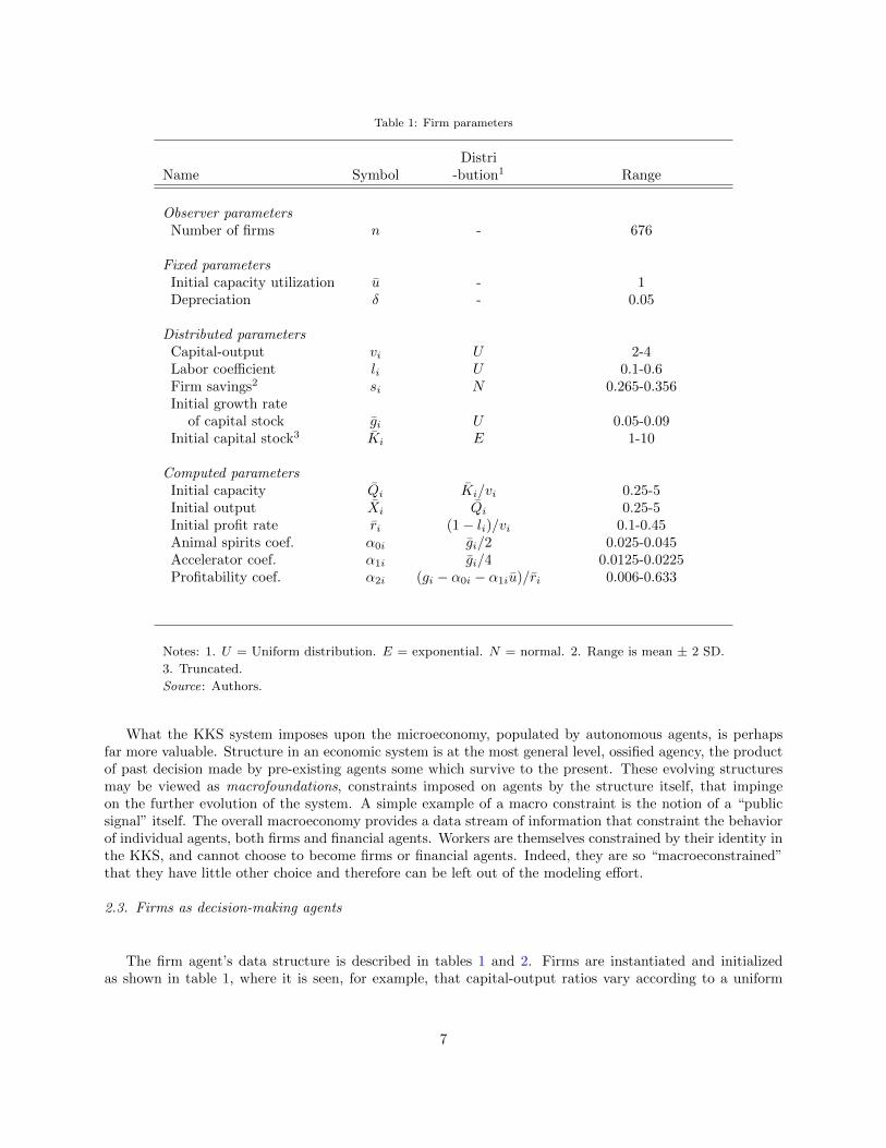
Table 1: Firm parameters

DistriName Symbol -bution1 Range

Observer parametersNumber of firms n - 676

Fixed parametersInitial capacity utilization u - 1Depreciation δ - 0.05

Distributed parametersCapital-output vi U 2-4Labor coefficient li U 0.1-0.6Firm savings2 si N 0.265-0.356Initial growth rate

of capital stock gi U 0.05-0.09Initial capital stock3 Ki E 1-10

Computed parametersInitial capacity Qi Ki/vi 0.25-5Initial output Xi Qi 0.25-5Initial profit rate ri (1− li)/vi 0.1-0.45Animal spirits coef. α0i gi/2 0.025-0.045Accelerator coef. α1i gi/4 0.0125-0.0225Profitability coef. α2i (gi − α0i − α1iu)/ri 0.006-0.633

Notes: 1. U = Uniform distribution. E = exponential. N = normal. 2. Range is mean ± 2 SD.

3. Truncated.

Source: Authors.

What the KKS system imposes upon the microeconomy, populated by autonomous agents, is perhapsfar more valuable. Structure in an economic system is at the most general level, ossified agency, the productof past decision made by pre-existing agents some which survive to the present. These evolving structuresmay be viewed as macrofoundations, constraints imposed on agents by the structure itself, that impingeon the further evolution of the system. A simple example of a macro constraint is the notion of a “publicsignal” itself. The overall macroeconomy provides a data stream of information that constraint the behaviorof individual agents, both firms and financial agents. Workers are themselves constrained by their identity inthe KKS, and cannot choose to become firms or financial agents. Indeed, they are so “macroeconstrained”that they have little other choice and therefore can be left out of the modeling effort.

2.3. Firms as decision-making agents

The firm agent’s data structure is described in tables 1 and 2. Firms are instantiated and initializedas shown in table 1, where it is seen, for example, that capital-output ratios vary according to a uniform

7

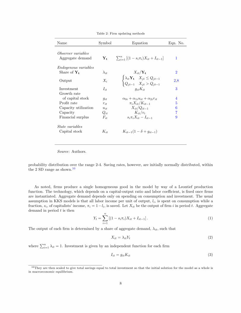
Table 2: Firm updating methods

Name Symbol Equation Eqn. No.

Observer variablesAggregate demand Yt

∑ni=1 [(1− siπi)Xit + Iit−1] 1

Endogenous variablesShare of Yt λit Xit/Yt 2

Output Xi

{λitYt Xjt ≤ Qjt−1

Qjt−1 Xjt > Qjt−1

2,8

Investment Iit gitKit 3Growth rate

of capital stock git α0i + α1iuit + α2irit 4Profit rate rit πiXit/Kit−1 5Capacity utilization uit Xit/Qit−1 6Capacity Qit Kit/vi 7Financial surplus Fit siπiXit − Iit−1 9

State variablesCapital stock Kit Kit−1(1− δ + git−1)

Source: Authors.

probability distribution over the range 2-4. Saving rates, however, are initially normally distributed, withinthe 2 SD range as shown.10

As noted, firms produce a single homogeneous good in the model by way of a Leontief productionfunction. The technology, which depends on a capital-output ratio and labor coefficient, is fixed once firmsare instantiated. Aggregate demand depends only on spending on consumption and investment. The usualassumption in KKS models is that all labor income per unit of output, li, is spent on consumption while afraction, si, of capitalists’ income, πi = 1− li, is saved. Let Xit be the output of firm i in period t. Aggregatedemand in period t is then

Yt =

n∑i=1

[(1− siπi)Xit + Iit−1] . (1)

The output of each firm is determined by a share of aggregate demand, λit, such that

Xit = λitYt (2)

where∑ni=1 λit = 1. Investment is given by an independent function for each firm

Iit = gitKit (3)

10They are then scaled to give total savings equal to total investment so that the initial solution for the model as a whole isin macroeconomic equilibrium.

8

where Kit denotes the capital stock and git is an accumulation function that depends on animal spirits,capacity utilization, and the rate of profit, or

git = α0i + α1iuit + α2irit (4)

where the a’s are constants and the rate of profit is

rit = πiXit/Kit−1. (5)

The values assigned to the parameters of this equation are shown in the lower part of table 1. The animalspirits term, α0i, is fixed for each firm, but given the randomness of other settings in the model animal spiritsis uncorrelated with any of the endogenous variables of the model.

It might seem more natural to model the firm in its traditional role of profit maximizer, combing thefactors of production in variable proportions to achieve least cost per unit of output. In fact, technicalefficiency in the multi-agent perspective is second order and it is rather the interaction of many firms andfinancial agents that attracts the attention of the agent-based method.

The methods by which firms update their data structures are shown in table 2. The basic rationalitybehind the firm’s decision-making is to increase (rather than maximize) profits by investing, creating produc-tive capacity through capital accumulation. This avoids loss of market share because of capacity constraints.When firms are capacity constrained, aggregate demand they cannot satisfy is allocated to other firms in aniterative processes within each sweep of the model, described in more detail below.

Capacity utilization, uit, is the firm’s variable that signals the need for more or less investment and isdefined as

uit = Xit/Qit−1 (6)

where and capacity output, Qit, isQit = Kit/vi (7)

where Kit is a state variable determined by the usual stock- flow relationship, as shown in table 2. Here Qitis the maximum quantity of production given the capital stock, Kit. Thus

Xit ≤ Qit−1 (8)

or equivalently, uit ≤ 1. Firms adapt to changes in the utilization of capacity by adjusting their rate ofinvestment.11

Note that there are, implicitly, multiple layers of decision-making for the firm agent. Entailed in thebehavior of the firm are incomes, both of workers and owners. Consumer behavior depends on these incomesand so indirectly depends on firm agents. Aggregate demand depends on the sum of these indirect effectstogether with the exogenous component of animal spirits in the investment function.

Typically, an agent-based model would take advantage of this multi-layered structure to endow theconsumers with their own choice points. Consumers may respond to spacial availability and price as they doin Gaffeo et al. [9]. They may decide to quit or change jobs, to accumulate human capital, retire, emigrateor join the informal sector [11]. In the hybrid model of this paper, these decisions are all directly linked, asthey are in the KKS framework, to the decision to invest.

Here the system-wide distribution of aggregate demand endows each firm with a quantity of savings thatmay or may not be sufficient to finance its planned investment. Inter-agent communication for firms dependson the financial surplus, Fit, defined as

Fit = siπiXit − Iit−1

< 0 deficit

= 0 balanced

> 0 surplus

(9)

11Since the rate of profit can also be written as rit = πiuit/vit, equation 4 is a function of the single signaling variable, uit.

9

for i = 1, 2, ..., n. The designation of surplus/deficit is temporary and depends on t, since in order to executeplanned investment, a deficit firm must first locate a surplus firm from which to borrow. If this provesimpossible, the deficit firm flips to surplus, as described in more detail below, and aggregate demand falls.In a model with perfect information, zero transactions costs, and endogenous money, nothing inhibits the flowof funds from surplus to deficit firms. Inter-agent communication is fast, effective, costless and complete. Inreallocation economies, however, interagent communications is less perfect and may breakdown, potentiallyreducing aggregate demand bringing about real-financial crisis.

2.4. The coordination environment of firm agents

Productive capacity is a state variable in the model, evolving along with the capital stock. In the currentmodel, capacity, Qi, may limit the amount of savings a firm generates, causing a surplus firm to flip andbecome a deficit firm.

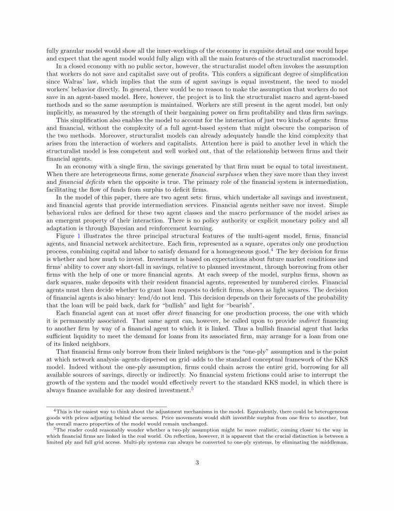
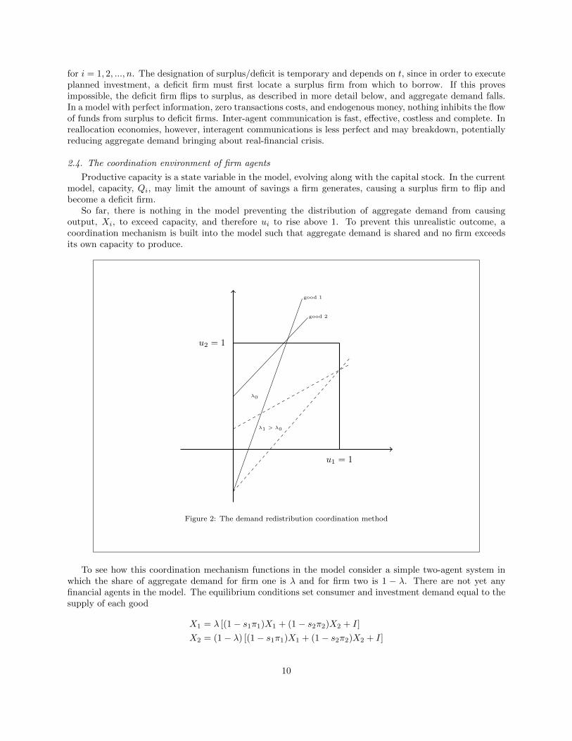
So far, there is nothing in the model preventing the distribution of aggregate demand from causingoutput, Xi, to exceed capacity, and therefore ui to rise above 1. To prevent this unrealistic outcome, acoordination mechanism is built into the model such that aggregate demand is shared and no firm exceedsits own capacity to produce.

u2 = 1

u1 = 1

good 1

good 2

λ0

λ1 > λ0

Figure 2: The demand redistribution coordination method

To see how this coordination mechanism functions in the model consider a simple two-agent system inwhich the share of aggregate demand for firm one is λ and for firm two is 1 − λ. There are not yet anyfinancial agents in the model. The equilibrium conditions set consumer and investment demand equal to thesupply of each good

X1 = λ [(1− s1π1)X1 + (1− s2π2)X2 + I]

X2 = (1− λ) [(1− s1π1)X1 + (1− s2π2)X2 + I]

10

Since u2 > 11. set u2 = 12. set Y (u1, u2) = Y (u1, 1)3. set u1 = λY (u1, 1)

4. reset λ = u1/∑2j=1 uj

5. if u1 ≤ 1 and u2 ≤ 1 haltelse repeat for u1 > 1

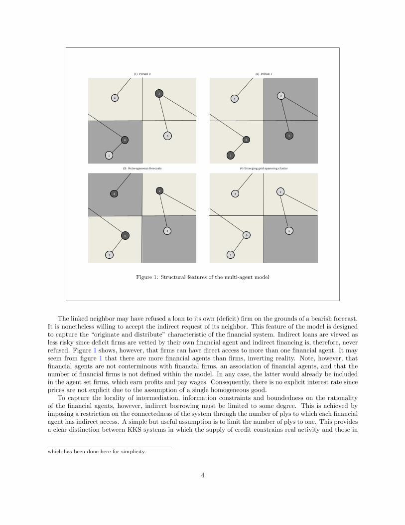
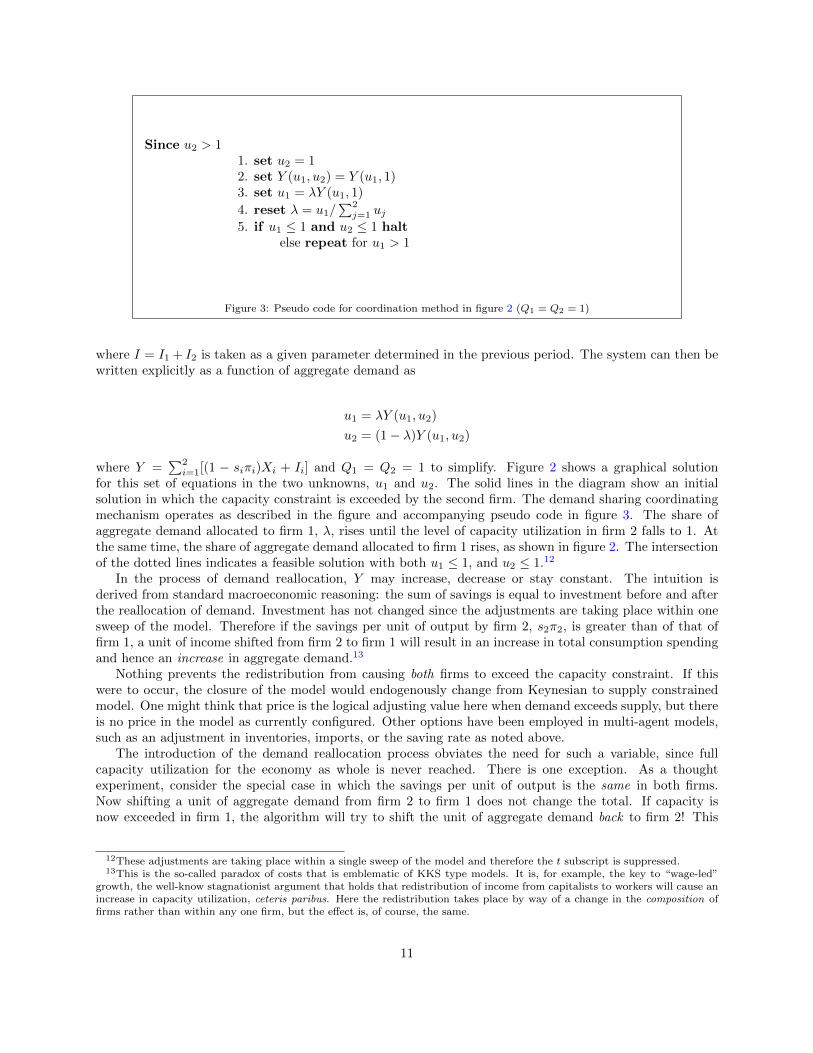
Figure 3: Pseudo code for coordination method in figure 2 (Q1 = Q2 = 1)

where I = I1 + I2 is taken as a given parameter determined in the previous period. The system can then bewritten explicitly as a function of aggregate demand as

u1 = λY (u1, u2)

u2 = (1− λ)Y (u1, u2)

where Y =∑2i=1[(1 − siπi)Xi + Ii] and Q1 = Q2 = 1 to simplify. Figure 2 shows a graphical solution

for this set of equations in the two unknowns, u1 and u2. The solid lines in the diagram show an initialsolution in which the capacity constraint is exceeded by the second firm. The demand sharing coordinatingmechanism operates as described in the figure and accompanying pseudo code in figure 3. The share ofaggregate demand allocated to firm 1, λ, rises until the level of capacity utilization in firm 2 falls to 1. Atthe same time, the share of aggregate demand allocated to firm 1 rises, as shown in figure 2. The intersectionof the dotted lines indicates a feasible solution with both u1 ≤ 1, and u2 ≤ 1.12

In the process of demand reallocation, Y may increase, decrease or stay constant. The intuition isderived from standard macroeconomic reasoning: the sum of savings is equal to investment before and afterthe reallocation of demand. Investment has not changed since the adjustments are taking place within onesweep of the model. Therefore if the savings per unit of output by firm 2, s2π2, is greater than of that offirm 1, a unit of income shifted from firm 2 to firm 1 will result in an increase in total consumption spendingand hence an increase in aggregate demand.13

Nothing prevents the redistribution from causing both firms to exceed the capacity constraint. If thiswere to occur, the closure of the model would endogenously change from Keynesian to supply constrainedmodel. One might think that price is the logical adjusting value here when demand exceeds supply, but thereis no price in the model as currently configured. Other options have been employed in multi-agent models,such as an adjustment in inventories, imports, or the saving rate as noted above.

The introduction of the demand reallocation process obviates the need for such a variable, since fullcapacity utilization for the economy as whole is never reached. There is one exception. As a thoughtexperiment, consider the special case in which the savings per unit of output is the same in both firms.Now shifting a unit of aggregate demand from firm 2 to firm 1 does not change the total. If capacity isnow exceeded in firm 1, the algorithm will try to shift the unit of aggregate demand back to firm 2! This

12These adjustments are taking place within a single sweep of the model and therefore the t subscript is suppressed.13This is the so-called paradox of costs that is emblematic of KKS type models. It is, for example, the key to “wage-led”

growth, the well-know stagnationist argument that holds that redistribution of income from capitalists to workers will cause anincrease in capacity utilization, ceteris paribus. Here the redistribution takes place by way of a change in the composition offirms rather than within any one firm, but the effect is, of course, the same.

11

chattering solution cannot be ruled out and in practice prevents the sweep from converging on a feasibledistribution of the ui.

14

There are a number of common elements of the agent-based approach that are intentionally ignored inthis treatment of the real side of the model. Firm agents could, for example, learn to combine factors ofproduction more efficiently, or invest in research and development to adjust their Leontief technologies, or usesophisticated models to forecast demand and therefore alter their investment decision away from equation4. None of these features is implemented in the current version of the model since this would diminishthe connection to the original KKS model, in particular the role of aggregate demand. Many are, however,implemented on the financial side. There, financial agents learn, communicate with one another, and forecastbehavior of other agents using sophisticated models, all of which can significantly affect firm investment.

2.5. Financial decision-making agents

The discussion of firm agents above has set the stage for the introduction of financial agents, who operatebetween surplus and deficit firms. The parameters defining this agent set are shown in table 3. While thereare n = 676 firms, the table indicates that there are m = 1, 000 financial agents, so that on average thereare approximately 1.5 financial agents per firm. Financial agents are randomly allocated to firms such thateach firm is linked to between one and 10 financial agents.

Each financial agent begins life with one unit of liquidity, their initial capitalization. To simplify matters,the capital stock of the firms to which each financial agent is randomly associated is the sum of the initialliquidity of the associated financial agents.15 Thereafter strict balance sheet consistency is imposed on finan-cial agents: since there is no currency or reserves, loans must be equal to deposits plus initial capitalization.Financial agents cannot fail or die; they can only run out of liquidity and must then refuse a loan request.

As noted above, financial agents only borrow to meet the needs of a deficit firm to which they couldnot otherwise provide financing. This approach differs from the traditional treatment as in Gai et al. [10],for example, in that this paper focuses primarily on bank intermediation, rather than whether banks canacquire needed liquidity through short-term interbank borrowing. Here there is no lender of last resort thatmight respond to a short-term liquidity crisis. Neither can financial agents freely create money.16

In the hybrid KKS model studied here, the decision financial agents make is whether to extend loansto deficit firms. This decision depends on two factors: availability of liquidity and willingness to lend.Conditional on having sufficient liquidity (direct finance) or access to liquidity through the interbank market(indirect finance), a financial agent will provide finance to a client firm if the financial agent is optimisticthat the value of these shares will rise over time. Financial agents make the decision to allow or disallowloans to deficit firms based on a relatively sophisticated forecast composed of two parts: a private signalbased on private information and a public signal, based on the forecasts of their linked neighbors, whichis public information. The relative weights the financial agents place on these two sources of informationchange depending upon the confidence they have in their own forecasting ability relative to that of linkedneighbors. Table 3 shows that the initial confidence is set at 0.5, which means that financial agents initiallyweigh private and public information equally.

14This would cause the simulation to be removed from the data.15Thus, a firm connected to two financial agents is instantiated with two units of capital and a firm with seven agents has

seven units of capital. An initial correlation of firm size, measured by their capital stock, with the number of financial agentsis then established.

16As explained in more detail below, money can be created but only when financial agents are forced to do so by theasynchronicity of the system.

12

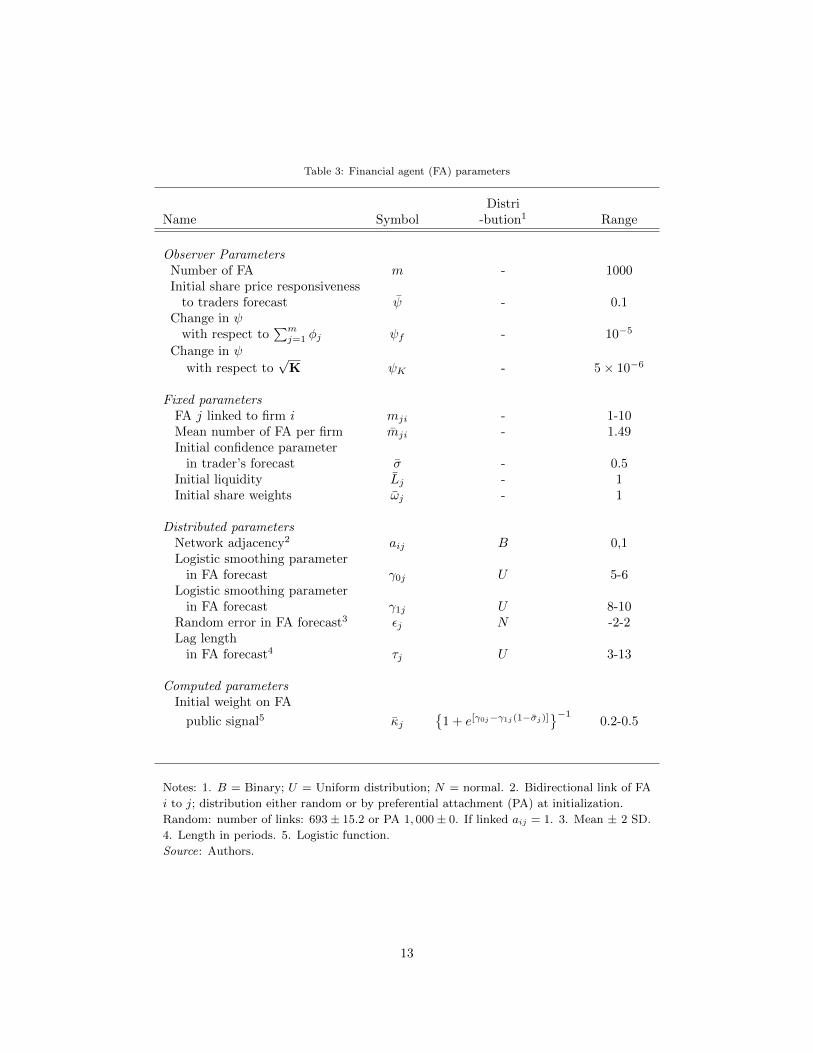
Table 3: Financial agent (FA) parameters

DistriName Symbol -bution1 Range

Observer ParametersNumber of FA m - 1000Initial share price responsiveness

to traders forecast ψ - 0.1Change in ψ

with respect to∑mj=1 φj ψf - 10−5

Change in ψ

with respect to√K ψK - 5× 10−6

Fixed parametersFA j linked to firm i mji - 1-10Mean number of FA per firm mji - 1.49Initial confidence parameter

in trader’s forecast σ - 0.5Initial liquidity Lj - 1Initial share weights ωj - 1

Distributed parametersNetwork adjacency2 aij B 0,1Logistic smoothing parameter

in FA forecast γ0j U 5-6Logistic smoothing parameter

in FA forecast γ1j U 8-10Random error in FA forecast3 εj N -2-2Lag length

in FA forecast4 τj U 3-13

Computed parametersInitial weight on FA

public signal5 κj{

1 + e[γ0j−γ1j(1−σj)]}−1

0.2-0.5

Notes: 1. B = Binary; U = Uniform distribution; N = normal. 2. Bidirectional link of FA

i to j; distribution either random or by preferential attachment (PA) at initialization.

Random: number of links: 693 ± 15.2 or PA 1, 000 ± 0. If linked aij = 1. 3. Mean ± 2 SD.

4. Length in periods. 5. Logistic function.

Source: Authors.

13

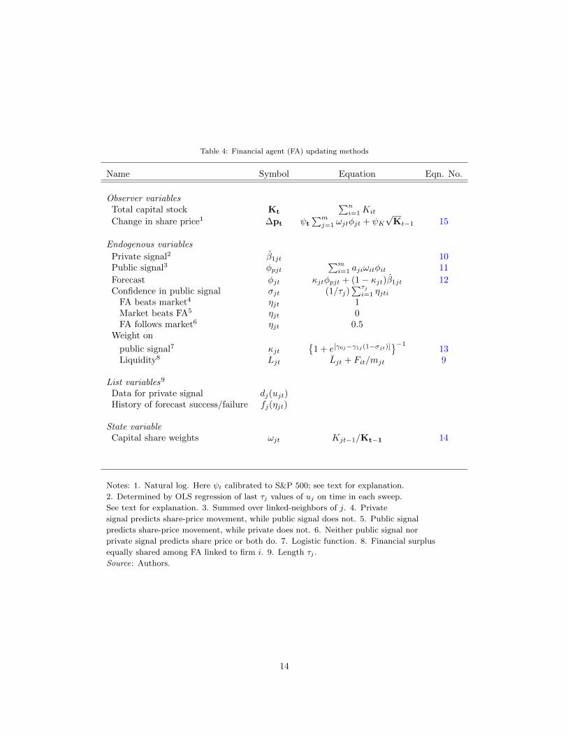
Table 4: Financial agent (FA) updating methods

Name Symbol Equation Eqn. No.

Observer variablesTotal capital stock Kt

∑ni=1Kit

Change in share price1 ∆pt ψt

∑mj=1 ωjtφjt + ψK

√Kt−1 15

Endogenous variables

Private signal2 β1jt 10Public signal3 φpjt

∑mi=1 ajiωitφit 11

Forecast φjt κjtφpjt + (1− κjt)β1jt 12Confidence in public signal σjt (1/τj)

∑τji=1 ηjti

FA beats market4 ηjt 1Market beats FA5 ηjt 0FA follows market6 ηjt 0.5

Weight on

public signal7 κjt{

1 + e[γ0j−γ1j(1−σjt)]}−1

13Liquidity8 Ljt Ljt + Fit/mjt 9

List variables9

Data for private signal dj(ujt)History of forecast success/failure fj(ηjt)

State variableCapital share weights ωjt Kjt−1/Kt−1 14

Notes: 1. Natural log. Here ψt calibrated to S&P 500; see text for explanation.

2. Determined by OLS regression of last τj values of uj on time in each sweep.

See text for explanation. 3. Summed over linked-neighbors of j. 4. Private

signal predicts share-price movement, while public signal does not. 5. Public signal

predicts share-price movement, while private does not. 6. Neither public signal nor

private signal predicts share price or both do. 7. Logistic function. 8. Financial surplus

equally shared among FA linked to firm i. 9. Length τj .

Source: Authors.

14

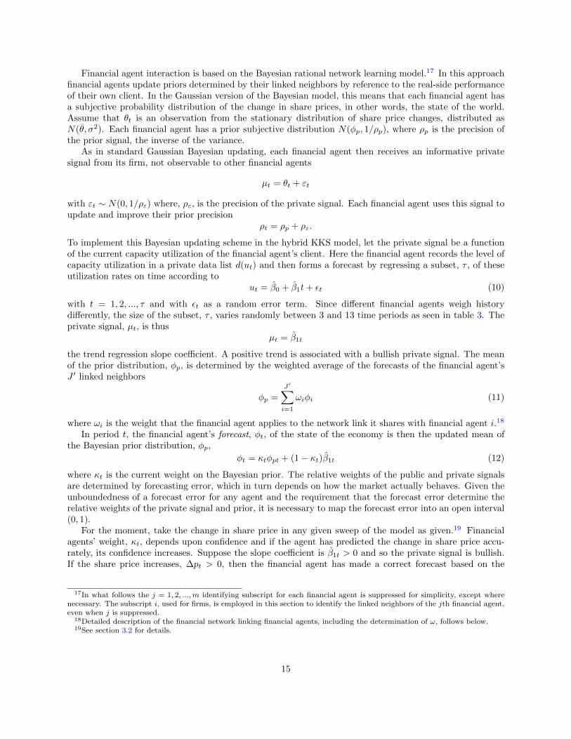
Financial agent interaction is based on the Bayesian rational network learning model.17 In this approachfinancial agents update priors determined by their linked neighbors by reference to the real-side performanceof their own client. In the Gaussian version of the Bayesian model, this means that each financial agent hasa subjective probability distribution of the change in share prices, in other words, the state of the world.Assume that θt is an observation from the stationary distribution of share price changes, distributed asN(θ, σ2). Each financial agent has a prior subjective distribution N(φp, 1/ρp), where ρp is the precision ofthe prior signal, the inverse of the variance.

As in standard Gaussian Bayesian updating, each financial agent then receives an informative privatesignal from its firm, not observable to other financial agents

µt = θt + εt

with εt ∼ N(0, 1/ρε) where, ρε, is the precision of the private signal. Each financial agent uses this signal toupdate and improve their prior precision

ρt = ρp + ρε.

To implement this Bayesian updating scheme in the hybrid KKS model, let the private signal be a functionof the current capacity utilization of the financial agent’s client. Here the financial agent records the level ofcapacity utilization in a private data list d(ut) and then forms a forecast by regressing a subset, τ , of theseutilization rates on time according to

ut = β0 + β1t+ εt (10)

with t = 1, 2, ..., τ and with εt as a random error term. Since different financial agents weigh historydifferently, the size of the subset, τ , varies randomly between 3 and 13 time periods as seen in table 3. Theprivate signal, µt, is thus

µt = β1t

the trend regression slope coefficient. A positive trend is associated with a bullish private signal. The meanof the prior distribution, φp, is determined by the weighted average of the forecasts of the financial agent’sJ ′ linked neighbors

φp =

J′∑i=1

ωiφi (11)

where ωi is the weight that the financial agent applies to the network link it shares with financial agent i.18

In period t, the financial agent’s forecast, φt, of the state of the economy is then the updated mean ofthe Bayesian prior distribution, φp,

φt = κtφpt + (1− κt)β1t (12)

where κt is the current weight on the Bayesian prior. The relative weights of the public and private signalsare determined by forecasting error, which in turn depends on how the market actually behaves. Given theunboundedness of a forecast error for any agent and the requirement that the forecast error determine therelative weights of the private signal and prior, it is necessary to map the forecast error into an open interval(0, 1).

For the moment, take the change in share price in any given sweep of the model as given.19 Financialagents’ weight, κt, depends upon confidence and if the agent has predicted the change in share price accu-rately, its confidence increases. Suppose the slope coefficient is β1t > 0 and so the private signal is bullish.If the share price increases, ∆pt > 0, then the financial agent has made a correct forecast based on the

17In what follows the j = 1, 2, ...,m identifying subscript for each financial agent is suppressed for simplicity, except wherenecessary. The subscript i, used for firms, is employed in this section to identify the linked neighbors of the jth financial agent,even when j is suppressed.

18Detailed description of the financial network linking financial agents, including the determination of ω, follows below.19See section 3.2 for details.

15

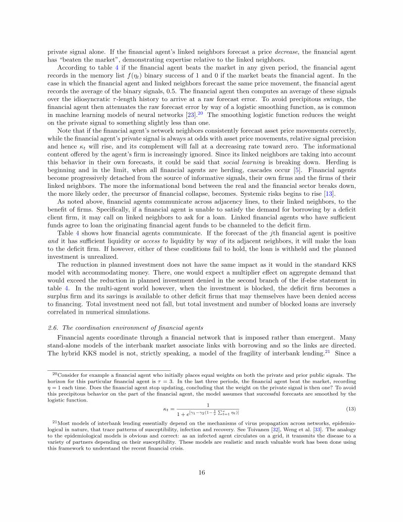
private signal alone. If the financial agent’s linked neighbors forecast a price decrease, the financial agenthas “beaten the market”, demonstrating expertise relative to the linked neighbors.

According to table 4 if the financial agent beats the market in any given period, the financial agentrecords in the memory list f(ηt) binary success of 1 and 0 if the market beats the financial agent. In thecase in which the financial agent and linked neighbors forecast the same price movement, the financial agentrecords the average of the binary signals, 0.5. The financial agent then computes an average of these signalsover the idiosyncratic τ -length history to arrive at a raw forecast error. To avoid precipitous swings, thefinancial agent then attenuates the raw forecast error by way of a logistic smoothing function, as is commonin machine learning models of neural networks [23].20 The smoothing logistic function reduces the weighton the private signal to something slightly less than one.

Note that if the financial agent’s network neighbors consistently forecast asset price movements correctly,while the financial agent’s private signal is always at odds with asset price movements, relative signal precisionand hence κt will rise, and its complement will fall at a decreasing rate toward zero. The informationalcontent offered by the agent’s firm is increasingly ignored. Since its linked neighbors are taking into accountthis behavior in their own forecasts, it could be said that social learning is breaking down. Herding isbeginning and in the limit, when all financial agents are herding, cascades occur [5]. Financial agentsbecome progressively detached from the source of informative signals, their own firms and the firms of theirlinked neighbors. The more the informational bond between the real and the financial sector breaks down,the more likely order, the precursor of financial collapse, becomes. Systemic risks begins to rise [13].

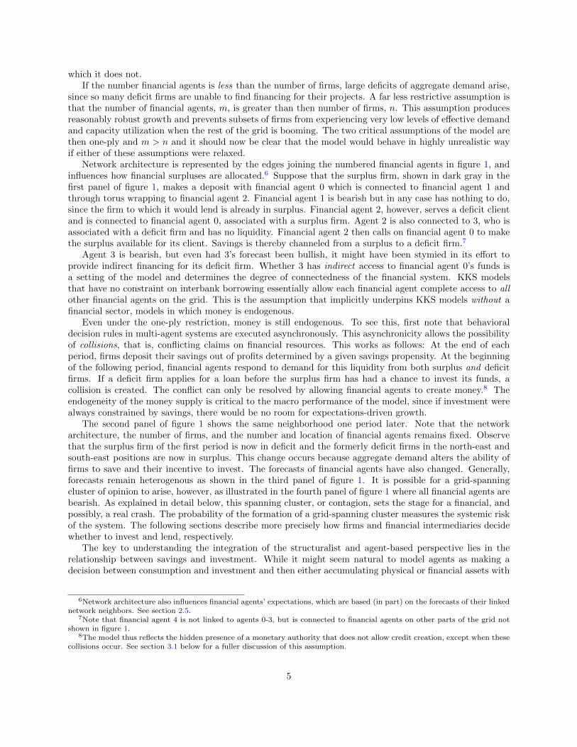
As noted above, financial agents communicate across adjacency lines, to their linked neighbors, to thebenefit of firms. Specifically, if a financial agent is unable to satisfy the demand for borrowing by a deficitclient firm, it may call on linked neighbors to ask for a loan. Linked financial agents who have sufficientfunds agree to loan the originating financial agent funds to be channeled to the deficit firm.

Table 4 shows how financial agents communicate. If the forecast of the jth financial agent is positiveand it has sufficient liquidity or access to liquidity by way of its adjacent neighbors, it will make the loanto the deficit firm. If however, either of these conditions fail to hold, the loan is withheld and the plannedinvestment is unrealized.

The reduction in planned investment does not have the same impact as it would in the standard KKSmodel with accommodating money. There, one would expect a multiplier effect on aggregate demand thatwould exceed the reduction in planned investment denied in the second branch of the if-else statement intable 4. In the multi-agent world however, when the investment is blocked, the deficit firm becomes asurplus firm and its savings is available to other deficit firms that may themselves have been denied accessto financing. Total investment need not fall, but total investment and number of blocked loans are inverselycorrelated in numerical simulations.

2.6. The coordination environment of financial agents

Financial agents coordinate through a financial network that is imposed rather than emergent. Manystand-alone models of the interbank market associate links with borrowing and so the links are directed.The hybrid KKS model is not, strictly speaking, a model of the fragility of interbank lending.21 Since a

20Consider for example a financial agent who initially places equal weights on both the private and prior public signals. Thehorizon for this particular financial agent is τ = 3. In the last three periods, the financial agent beat the market, recordingη = 1 each time. Does the financial agent stop updating, concluding that the weight on the private signal is then one? To avoidthis precipitous behavior on the part of the financial agent, the model assumes that successful forecasts are smoothed by thelogistic function.

κt =1

1 + e[γ1−γ2(1−1τ

∑τt=1 ηt)]

(13)

21Most models of interbank lending essentially depend on the mechanisms of virus propagation across networks, epidemio-logical in nature, that trace patterns of susceptibility, infection and recovery. See Toivanen [32], Weng et al. [33]. The analogyto the epidemiological models is obvious and correct: as an infected agent circulates on a grid, it transmits the disease to avariety of partners depending on their susceptibility. These models are realistic and much valuable work has been done usingthis framework to understand the recent financial crisis.

16

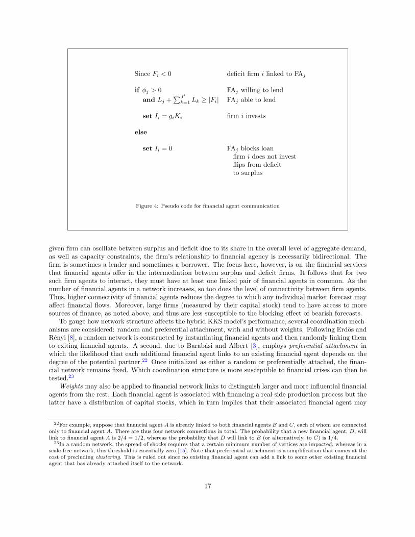
Since Fi < 0 deficit firm i linked to FAj

if φj > 0 FAj willing to lend

and Lj +∑J′

k=1 Lk ≥ |Fi| FAj able to lend

set Ii = giKi firm i invests

else

set Ii = 0 FAj blocks loanfirm i does not investflips from deficitto surplus

Figure 4: Pseudo code for financial agent communication

given firm can oscillate between surplus and deficit due to its share in the overall level of aggregate demand,as well as capacity constraints, the firm’s relationship to financial agency is necessarily bidirectional. Thefirm is sometimes a lender and sometimes a borrower. The focus here, however, is on the financial servicesthat financial agents offer in the intermediation between surplus and deficit firms. It follows that for twosuch firm agents to interact, they must have at least one linked pair of financial agents in common. As thenumber of financial agents in a network increases, so too does the level of connectivity between firm agents.Thus, higher connectivity of financial agents reduces the degree to which any individual market forecast mayaffect financial flows. Moreover, large firms (measured by their capital stock) tend to have access to moresources of finance, as noted above, and thus are less susceptible to the blocking effect of bearish forecasts.

To gauge how network structure affects the hybrid KKS model’s performance, several coordination mech-anisms are considered: random and preferential attachment, with and without weights. Following Erdos andRenyi [8], a random network is constructed by instantiating financial agents and then randomly linking themto exiting financial agents. A second, due to Barabasi and Albert [3], employs preferential attachment inwhich the likelihood that each additional financial agent links to an existing financial agent depends on thedegree of the potential partner.22 Once initialized as either a random or preferentially attached, the finan-cial network remains fixed. Which coordination structure is more susceptible to financial crises can then betested.23

Weights may also be applied to financial network links to distinguish larger and more influential financialagents from the rest. Each financial agent is associated with financing a real-side production process but thelatter have a distribution of capital stocks, which in turn implies that their associated financial agent may

22For example, suppose that financial agent A is already linked to both financial agents B and C, each of whom are connectedonly to financial agent A. There are thus four network connections in total. The probability that a new financial agent, D, willlink to financial agent A is 2/4 = 1/2, whereas the probability that D will link to B (or alternatively, to C) is 1/4.

23In a random network, the spread of shocks requires that a certain minimum number of vertices are impacted, whereas in ascale-free network, this threshold is essentially zero [15]. Note that preferential attachment is a simplification that comes at thecost of precluding clustering. This is ruled out since no existing financial agent can add a link to some other existing financialagent that has already attached itself to the network.

17

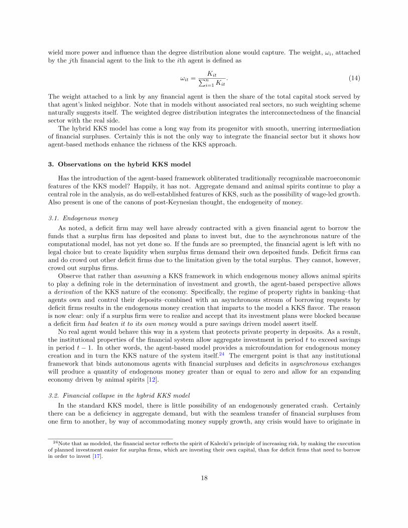
wield more power and influence than the degree distribution alone would capture. The weight, ωi, attachedby the jth financial agent to the link to the ith agent is defined as

ωit =Kit∑ni=1Kit

. (14)

The weight attached to a link by any financial agent is then the share of the total capital stock served bythat agent’s linked neighbor. Note that in models without associated real sectors, no such weighting schemenaturally suggests itself. The weighted degree distribution integrates the interconnectedness of the financialsector with the real side.

The hybrid KKS model has come a long way from its progenitor with smooth, unerring intermediationof financial surpluses. Certainly this is not the only way to integrate the financial sector but it shows howagent-based methods enhance the richness of the KKS approach.

3. Observations on the hybrid KKS model

Has the introduction of the agent-based framework obliterated traditionally recognizable macroeconomicfeatures of the KKS model? Happily, it has not. Aggregate demand and animal spirits continue to play acentral role in the analysis, as do well-established features of KKS, such as the possibility of wage-led growth.Also present is one of the canons of post-Keynesian thought, the endogeneity of money.

3.1. Endogenous money

As noted, a deficit firm may well have already contracted with a given financial agent to borrow thefunds that a surplus firm has deposited and plans to invest but, due to the asynchronous nature of thecomputational model, has not yet done so. If the funds are so preempted, the financial agent is left with nolegal choice but to create liquidity when surplus firms demand their own deposited funds. Deficit firms canand do crowd out other deficit firms due to the limitation given by the total surplus. They cannot, however,crowd out surplus firms.

Observe that rather than assuming a KKS framework in which endogenous money allows animal spiritsto play a defining role in the determination of investment and growth, the agent-based perspective allowsa derivation of the KKS nature of the economy. Specifically, the regime of property rights in banking–thatagents own and control their deposits–combined with an asynchronous stream of borrowing requests bydeficit firms results in the endogenous money creation that imparts to the model a KKS flavor. The reasonis now clear: only if a surplus firm were to realize and accept that its investment plans were blocked becausea deficit firm had beaten it to its own money would a pure savings driven model assert itself.

No real agent would behave this way in a system that protects private property in deposits. As a result,the institutional properties of the financial system allow aggregate investment in period t to exceed savingsin period t − 1. In other words, the agent-based model provides a microfoundation for endogenous moneycreation and in turn the KKS nature of the system itself.24 The emergent point is that any institutionalframework that binds autonomous agents with financial surpluses and deficits in asynchronous exchangeswill produce a quantity of endogenous money greater than or equal to zero and allow for an expandingeconomy driven by animal spirits [12].

3.2. Financial collapse in the hybrid KKS model

In the standard KKS model, there is little possibility of an endogenously generated crash. Certainlythere can be a deficiency in aggregate demand, but with the seamless transfer of financial surpluses fromone firm to another, by way of accommodating money supply growth, any crisis would have to originate in

24Note that as modeled, the financial sector reflects the spirit of Kalecki’s principle of increasing risk, by making the executionof planned investment easier for surplus firms, which are investing their own capital, than for deficit firms that need to borrowin order to invest [17].

18

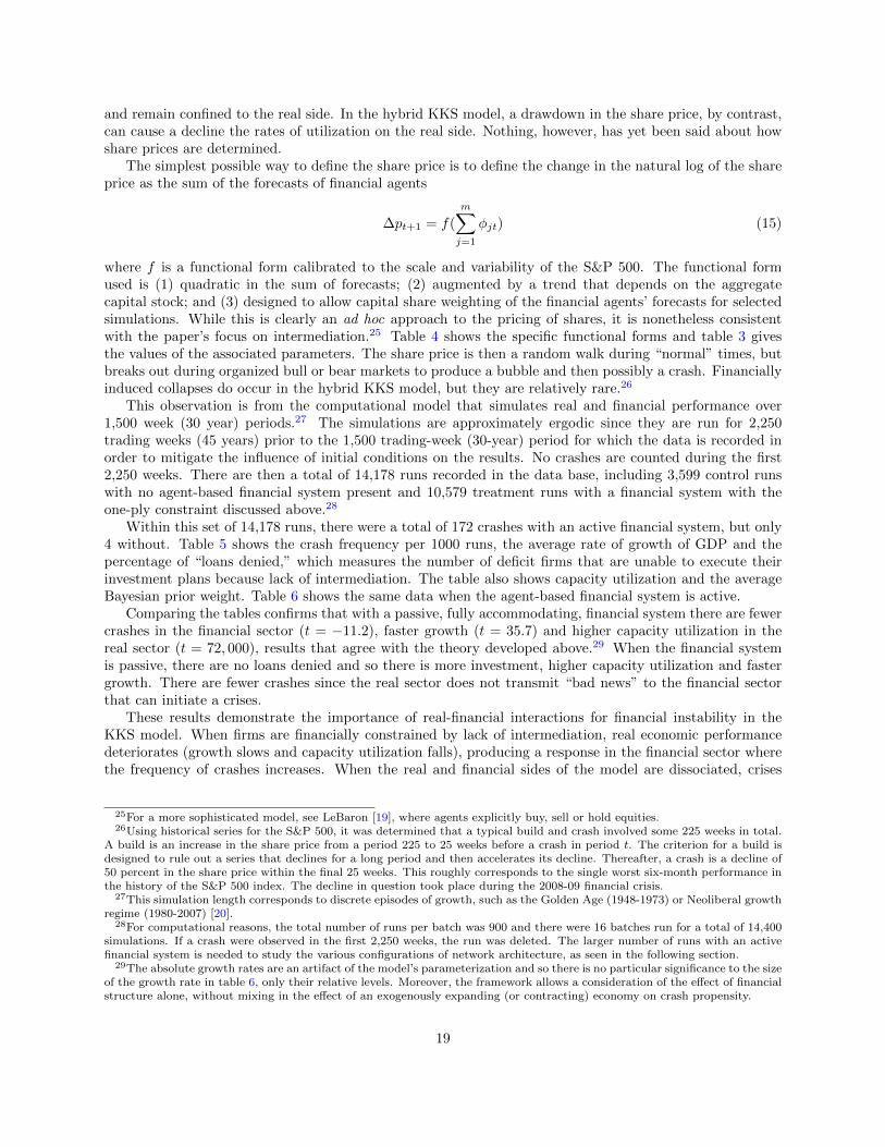
and remain confined to the real side. In the hybrid KKS model, a drawdown in the share price, by contrast,can cause a decline the rates of utilization on the real side. Nothing, however, has yet been said about howshare prices are determined.

The simplest possible way to define the share price is to define the change in the natural log of the shareprice as the sum of the forecasts of financial agents

∆pt+1 = f(

m∑j=1

φjt) (15)

where f is a functional form calibrated to the scale and variability of the S&P 500. The functional formused is (1) quadratic in the sum of forecasts; (2) augmented by a trend that depends on the aggregatecapital stock; and (3) designed to allow capital share weighting of the financial agents’ forecasts for selectedsimulations. While this is clearly an ad hoc approach to the pricing of shares, it is nonetheless consistentwith the paper’s focus on intermediation.25 Table 4 shows the specific functional forms and table 3 givesthe values of the associated parameters. The share price is then a random walk during “normal” times, butbreaks out during organized bull or bear markets to produce a bubble and then possibly a crash. Financiallyinduced collapses do occur in the hybrid KKS model, but they are relatively rare.26

This observation is from the computational model that simulates real and financial performance over1,500 week (30 year) periods.27 The simulations are approximately ergodic since they are run for 2,250trading weeks (45 years) prior to the 1,500 trading-week (30-year) period for which the data is recorded inorder to mitigate the influence of initial conditions on the results. No crashes are counted during the first2,250 weeks. There are then a total of 14,178 runs recorded in the data base, including 3,599 control runswith no agent-based financial system present and 10,579 treatment runs with a financial system with theone-ply constraint discussed above.28

Within this set of 14,178 runs, there were a total of 172 crashes with an active financial system, but only4 without. Table 5 shows the crash frequency per 1000 runs, the average rate of growth of GDP and thepercentage of “loans denied,” which measures the number of deficit firms that are unable to execute theirinvestment plans because lack of intermediation. The table also shows capacity utilization and the averageBayesian prior weight. Table 6 shows the same data when the agent-based financial system is active.

Comparing the tables confirms that with a passive, fully accommodating, financial system there are fewercrashes in the financial sector (t = −11.2), faster growth (t = 35.7) and higher capacity utilization in thereal sector (t = 72, 000), results that agree with the theory developed above.29 When the financial systemis passive, there are no loans denied and so there is more investment, higher capacity utilization and fastergrowth. There are fewer crashes since the real sector does not transmit “bad news” to the financial sectorthat can initiate a crises.

These results demonstrate the importance of real-financial interactions for financial instability in theKKS model. When firms are financially constrained by lack of intermediation, real economic performancedeteriorates (growth slows and capacity utilization falls), producing a response in the financial sector wherethe frequency of crashes increases. When the real and financial sides of the model are dissociated, crises

25For a more sophisticated model, see LeBaron [19], where agents explicitly buy, sell or hold equities.26Using historical series for the S&P 500, it was determined that a typical build and crash involved some 225 weeks in total.

A build is an increase in the share price from a period 225 to 25 weeks before a crash in period t. The criterion for a build isdesigned to rule out a series that declines for a long period and then accelerates its decline. Thereafter, a crash is a decline of50 percent in the share price within the final 25 weeks. This roughly corresponds to the single worst six-month performance inthe history of the S&P 500 index. The decline in question took place during the 2008-09 financial crisis.

27This simulation length corresponds to discrete episodes of growth, such as the Golden Age (1948-1973) or Neoliberal growthregime (1980-2007) [20].

28For computational reasons, the total number of runs per batch was 900 and there were 16 batches run for a total of 14,400simulations. If a crash were observed in the first 2,250 weeks, the run was deleted. The larger number of runs with an activefinancial system is needed to study the various configurations of network architecture, as seen in the following section.

29The absolute growth rates are an artifact of the model’s parameterization and so there is no particular significance to the sizeof the growth rate in table 6, only their relative levels. Moreover, the framework allows a consideration of the effect of financialstructure alone, without mixing in the effect of an exogenously expanding (or contracting) economy on crash propensity.

19

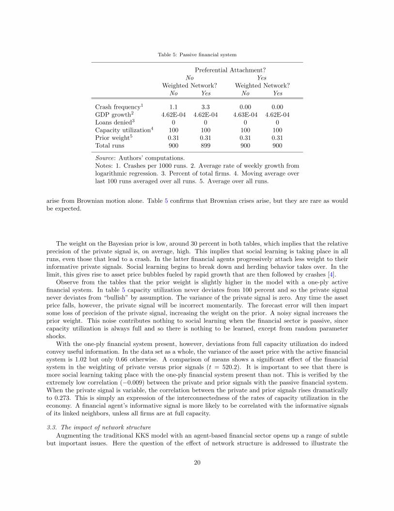
Table 5: Passive financial system

Preferential Attachment?No Yes

Weighted Network? Weighted Network?No Yes No Yes

Crash frequency1 1.1 3.3 0.00 0.00GDP growth2 4.62E-04 4.62E-04 4.63E-04 4.62E-04Loans denied3 0 0 0 0Capacity utilization4 100 100 100 100Prior weight5 0.31 0.31 0.31 0.31Total runs 900 899 900 900

Source: Authors’ computations.Notes: 1. Crashes per 1000 runs. 2. Average rate of weekly growth fromlogarithmic regression. 3. Percent of total firms. 4. Moving average overlast 100 runs averaged over all runs. 5. Average over all runs.

arise from Brownian motion alone. Table 5 confirms that Brownian crises arise, but they are rare as wouldbe expected.

The weight on the Bayesian prior is low, around 30 percent in both tables, which implies that the relativeprecision of the private signal is, on average, high. This implies that social learning is taking place in allruns, even those that lead to a crash. In the latter financial agents progressively attach less weight to theirinformative private signals. Social learning begins to break down and herding behavior takes over. In thelimit, this gives rise to asset price bubbles fueled by rapid growth that are then followed by crashes [4].

Observe from the tables that the prior weight is slightly higher in the model with a one-ply activefinancial system. In table 5 capacity utilization never deviates from 100 percent and so the private signalnever deviates from “bullish” by assumption. The variance of the private signal is zero. Any time the assetprice falls, however, the private signal will be incorrect momentarily. The forecast error will then impartsome loss of precision of the private signal, increasing the weight on the prior. A noisy signal increases theprior weight. This noise contributes nothing to social learning when the financial sector is passive, sincecapacity utilization is always full and so there is nothing to be learned, except from random parametershocks.

With the one-ply financial system present, however, deviations from full capacity utilization do indeedconvey useful information. In the data set as a whole, the variance of the asset price with the active financialsystem is 1.02 but only 0.66 otherwise. A comparison of means shows a significant effect of the financialsystem in the weighting of private versus prior signals (t = 520.2). It is important to see that there ismore social learning taking place with the one-ply financial system present than not. This is verified by theextremely low correlation (−0.009) between the private and prior signals with the passive financial system.When the private signal is variable, the correlation between the private and prior signals rises dramaticallyto 0.273. This is simply an expression of the interconnectedness of the rates of capacity utilization in theeconomy. A financial agent’s informative signal is more likely to be correlated with the informative signalsof its linked neighbors, unless all firms are at full capacity.

3.3. The impact of network structure

Augmenting the traditional KKS model with an agent-based financial sector opens up a range of subtlebut important issues. Here the question of the effect of network structure is addressed to illustrate the

20

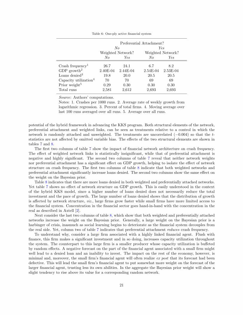
Table 6: One-ply active financial system

Preferential Attachment?No Yes

Weighted Network? Weighted Network?No Yes No Yes

Crash frequency1 26.7 24.1 6.7 8.2GDP growth2 2.40E-04 2.44E-04 2.54E-04 2.53E-04Loans denied3 19.8 20.0 20.5 20.5Capacity utilization4 70 70 69 69Prior weight5 0.29 0.30 0.30 0.30Total runs 2,581 2,612 2,693 2,693

Source: Authors’ computations.Notes: 1. Crashes per 1000 runs. 2. Average rate of weekly growth fromlogarithmic regression. 3. Percent of total firms. 4. Moving average overlast 100 runs averaged over all runs. 5. Average over all runs.

potential of the hybrid framework in advancing the KKS program. Both structural elements of the network,preferential attachment and weighted links, can be seen as treatments relative to a control in which thenetwork is randomly attached and unweighted. The treatments are uncorrelated (−0.004) so that the t-statistics are not affected by omitted variable bias. The effects of the two structural elements are shown intables 7 and 8.

The first two columns of table 7 show the impact of financial network architecture on crash frequency.The effect of weighted network links is statistically insignificant, while that of preferential attachment isnegative and highly significant. The second two columns of table 7 reveal that neither network weightsnor preferential attachment has a significant effect on GDP growth, helping to isolate the effect of networkstructure on crash frequency. The first two columns of table 8 indicate that both weighted networks andpreferential attachment significantly increase loans denied. The second two columns show the same effect onthe weight on the Bayesian prior.

Table 8 indicates that there are more loans denied in both weighted and preferentially attached networks.Yet table 7 shows no effect of network structure on GDP growth. This is easily understood in the contextof the hybrid KKS model, since a higher number of loans denied does not necessarily reduce the totalinvestment and the pace of growth. The large number of loans denied shows that the distribution of growthis affected by network structure, viz., large firms grow faster while small firms have more limited access tothe financial system. Concentration in the financial sector goes hand-in-hand with the concentration in thereal as described in Axtell [2].

Next consider the last two columns of table 8, which show that both weighted and preferentially attachednetworks increase the weight on the Bayesian prior. Generally, a large weight on the Bayesian prior is aharbinger of crisis, inasmuch as social learning begins to deteriorate as the financial system decouples fromthe real side. Yet, column two of table 7 indicates that preferential attachment reduces crash frequency.

To understand why, consider a large firm associated with a highly linked financial agent. Flush withfinance, this firm makes a significant investment and in so doing, increases capacity utilization throughoutthe system. The counterpart to this large firm is a smaller producer whose capacity utilization is buffetedby random effects. A negative forecast on the part of the financial agent associated with a small firm mightwell lead to a denied loan and an inability to invest. The impact on the rest of the economy, however, isminimal and, moreover, the small firm’s financial agent will often realize ex post that its forecast had beendefective. This will lead the small firm’s financial agent to put somewhat more weight on the forecast of thelarger financial agent, trusting less its own abilities. In the aggregate the Bayesian prior weight will show aslight tendency to rise above its value for a corresponding random network.

21

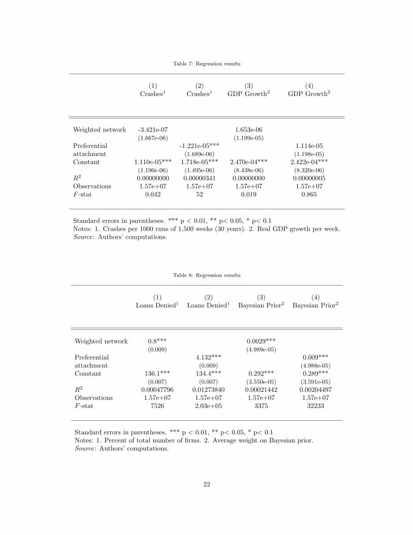
Table 7: Regression results

(1) (2) (3) (4)Crashes1 Crashes1 GDP Growth2 GDP Growth2

Weighted network -3.421e-07 1.653e-06(1.667e-06) (1.199e-05)

Preferential -1.221e-05*** 1.114e-05attachment (1.689e-06) (1.198e-05)

Constant 1.110e-05*** 1.718e-05*** 2.470e-04*** 2.422e-04***(1.190e-06) (1.495e-06) (8.438e-06) (8.320e-06)

R2 0.00000000 0.00000341 0.00000000 0.00000005Observations 1.57e+07 1.57e+07 1.57e+07 1.57e+07F -stat 0.042 52 0.019 0.865

Standard errors in parentheses. *** p < 0.01, ** p< 0.05, * p< 0.1Notes: 1. Crashes per 1000 runs of 1,500 weeks (30 years). 2. Real GDP growth per week.Source: Authors’ computations.

Table 8: Regression results

(1) (2) (3) (4)Loans Denied1 Loans Denied1 Bayesian Prior2 Bayesian Prior2

Weighted network 0.8*** 0.0029***(0.009) (4.989e-05)

Preferential 4.132*** 0.009***attachment (0.009) (4.988e-05)

Constant 136.1*** 134.4*** 0.292*** 0.289***(0.007) (0.007) (3.550e-05) (3.591e-05)

R2 0.00047796 0.01273840 0.00021442 0.00204497Observations 1.57e+07 1.57e+07 1.57e+07 1.57e+07F -stat 7526 2.03e+05 3375 32233

Standard errors in parentheses. *** p < 0.01, ** p< 0.05, * p< 0.1Notes: 1. Percent of total number of firms. 2. Average weight on Bayesian prior.Source: Authors’ computations.

22

In this case, the rise in the Bayesian prior weight does not imply a decoupling of the financial from thereal sector, however, and social learning is in fact enhanced. Financial agents are simply learning to pay moreattention to those firms who have greater impact on the macroeconomy as a whole. Crash frequency, forthese reasons, declines with preferential attachment. Preferential attachment, at least under the assumptionsof the present model, does not appear to increase systemic risk.

4. Conclusions

The central message of the paper is that the traditional KKS model and the agent-based methodology arenot necessarily “strange bed-fellows.” The multi-agent perspective confers a number of analytical advantagesas developed in this paper. First, it allows a non-standard microfoundation for the KKS model that is notbased on the representative agent maximizing an inter- temporal utility function. Heterogenous agentson both the real and financial sides operate with bounded rationality in an informationally constrainedenvironment. Second, the inclusion of an agent-based financial system allows a deep integration of thetreatment of intermediation with the fundamental problem of aggregate demand, endogenous money, andthe balance between savings and investment, all central themes of the KKS program. In this sense thetraditional KKS model with a passive financial sector simply ignores much of rich texture that has emergedas financial markets have become more sophisticated. Kregel [18] argued that Keynesian real-side modelswith no monetary and financial sectors were akin to “Hamlet without the prince” and this paper shows oneway in which this shortcoming can be addressed.

Setterfield and Budd [24] was a first attempt to develop a hybrid KKS model, but there were problemsin the the demand sharing algorithm that essentially converted the framework into a trade model, with eachfirm behaving as if it were a country. Other papers, have dealt with the problem of full capacity utilizationin various ways. This paper proposes a novel approach to aggregate demand sharing that eliminates theproblem that a firm might exceed full capacity utilization. The method is simple and broadly correspondsto the idea that when consumers (or investors) cannot find what they need in one location, the demandspills over to another. As seen, this algorithm can instantaneously change a surplus to a deficit firm andvice-versa. It also preserves basic KKS concepts such as animal spirits and aggregate demand, features thatare easily obscured in the agent-based approach.

Two important insights arise from the integration of KKS and the agent-based perspective. First, modelsthat focus on financial crises from an epidemiological perspective have been successful in showing how a highlyconnected system of interbank lending can facilitate the propagation of financial disturbances. As importantas these models have been, however, they appear to be fundamentally incomplete. Banks can cause crisis,but unless that crisis is validated by a real-side contraction in aggregate demand, that then reverberatesback into the financial system, the effect will not be as profound. The 1987 crash, for example, differedfundamentally from the recent 2008 financial crisis, which was an outgrowth of deep-seated problems in thehousing market. Second, while connectedness in previous models amplifies financial disturbance, the effectof preferential attachment here seems to be the reverse. A more connected financial system as it interactswith the real side is more resistant to financial disturbance and actually shows fewer crashes than its lessconnected counterpart. Since the model of this paper is so fundamentally different from those that dominatethe agent-based literature on financial crises, it is difficult to conclude that the latter are wrong. Instead,our results perhaps suggest that the complete story of real-financial interaction has yet to be told.

5. Appendix: Pseudo code

The program can be expressed as:

1. Initialize data structures and runtime options

2. Set key parameters

(a) Set share weights–boolean(b) Set preferential attachment–boolean(c) Set financial constraint–boolean

23

(d) Set run years–30 × 50 weeks

3. Set up and initialize network

4. Reassign financial agents such that each firm has at least one financial agent

5. Set shareholders as count financial agents for each firm

6. Initialize surplus of each firm based on randomly assigned parameters

7. Run main

8. If financial constraint = FALSE: set invest = TRUE for all firms

9. If financial constraint = TRUE:

(a) Ask financial agents: make forecast based on last period’s private and public signals(b) Ask firms: if surplus > 0 set invest = TRUE(c) Ask firms: if surplus < 0 ask one of financial agents if loanable funds |surplus|

i. If yes: set invest = TRUEii. If no: ask linked neighbor: if loanable funds > |surplus|

A. if yes: set invest = TRUEB. if no: set invest = FALSEC. update denied-loan counter

10. Run demand sharing algorithm [sum of investment of firms with invest = TRUE]

(a) Set demand shares of firms(b) Set capacity utilization of firms(c) Set savings of firms(d) Set planned investment(e) Set surpluses of firms(f) Set loanable funds = surpluses of surplus firms

11. If share-weight = TRUE

(a) Re-weight links by accumulated capital stocks

12. Stop for crash

13. Stop for year limit

14. Stop for capacity utilization lower limit (0.6)

15. Return to main

16. Process output

[1] Ashraf, Q., B. Gershman, and P. Howitt (2011, June). Banks, market organization, and macroeconomicperformance: An agent-based computational analysis. NBER Working Papers 17102, National Bureau ofEconomic Research, Inc.

[2] Axtell, R. (1999). The emergence of firms in a population of agents.http://www.brookings.edu/es/dynamics/papers/firms/firmspage.htm.

[3] Barabasi, A.-L. and R. Albert (1999). Emergence of scaling in random networks. Science 286, 509–512.

[4] Bikhchandani, S., D. Hirshleifer, and I. Welch (1998). Learning from the behavior of others: Conformity,fads, and informational cascades. The Journal of Economic Perspectives 12 (3), 151–170.

[5] Chamley, C. P. (2004). Rational Herds: Economic Models of Social Learning. Cambridge UniversityPress.

[6] Chick, V. (1983). Macroeconomics after Keynes: a reconsideration of the General Theory. Open accesspublications from University College London, University College London.

[7] Epstein, G. (2005). Financialization and the World Economy. Cheltenham, UK and Northampton, MA:Edward Elgar.

[8] Erdos, P. and A. Renyi (1950). On the evolution of random graphs. In Publication of the MathematicalInstitute of the Hungarian Academy of Sciences, pp. 17–61.

24

[9] Gaffeo, E., D. Delli Gatti, S. Desiderio, and M. Gallegati (2008). Adaptive microfoundations for emergentmacroeconomics. Eastern Econ Journal 34 (4), 441–463.

[10] Gai, P., A. Haldane, and S. Kapadia (2011). Complexity, concentration and contagion. Journal ofMonetary Economics 58 (5), 453–470.

[11] Gibson, B. (2012). Trade, employment and the informal sector: An agent-based analysis. The Margin:The Journal of Applied Economic Research 6 (2), 277–306.

[12] Gibson, B. and M. Setterfield (2015). Intermediation, money creation, and keynesian macrodynamicsin multi-agent systems. Technical report, University of Vermont.

[13] Hansen, L. P. (2012). Challenges in identifying and measuring systemic risk. Working Paper 18505,National Bureau of Economic Research.

[14] Harras, G. and D. Sornette (2011). How to grow a bubble: A model of myopic adapting agents. Journalof Economic Behavior & Organization 80 (1), 137–152.

[15] Iori, G., G. d. Masi, O. Precup, G. Gabbi, and G. Caldarelli (2008, January). A network analysis of theitalian overnight money market. Journal of Economic Dynamics and Control 32 (1), 259–278.

[16] Johansen, A., O. Ledoit, and D. Sornette (2000). Crashes as critical points. International Journal ofTheoretical and Applied Finance 3 (2), 219–255.

[17] Kalecki, M. (1937). The principle of increasing risk. Economica 4 (4), 440–446.

[18] Kregel, J. A. (1985). Hamlet without the prince: Cambridge macroeconomics without money. AmericanEconomic Review 75, 133–139.

[19] LeBaron, B. (2012). Heterogeneous gain learning and the dynamics of asset prices. Journal of EconomicBehavior & Organization 83 (3), 424–445.

[20] Maddison, A. (2007). The World Economy: A Millennial Perspective. Development Centre Studies.Paris: OECD Publishing.

[21] Palley, T. I. (2014). Financialization: The Economics of Finance Capital Domination. Palgrave Macmil-lan.

[22] Robertson, D. (1940). Effective demand the multiplier. In Essays in Monetary Theory. London: P.S.King.

[23] Russell, S. J. and P. Norvig (2010). Artificial Intelligence - A Modern Approach. New York: PearsonEducation.

[24] Setterfield, M. and A. Budd (2011). A Keynes-Kalecki model of cyclical growth with agent-basedfeatures. In P. Arestis (Ed.), Microeconomics, Macroeconomics and Economic Policy: Essays in Honourof Malcolm Sawyer, pp. 228–250. London and New York: Palgrave Macmillan.

[25] Skott, P. (2012, February). Pluralism, the lucas critique, and the integration of macro and micro.UMASS Amherst Economics Working Papers 2012-04, University of Massachusetts Amherst, Departmentof Economics.

[26] Sornette, D. (2003). Why Stock Markets Crash. Princeton, NJ: Princeton University Press.

[27] Taylor, L. (1981). IS/LM in the tropics : diagrammatics of the new structuralist macro critique. InW. R. Cline (Ed.), Economic stabilization in developing countries., pp. 465–503. Brookings Institution.

[28] Taylor, L. (1983). Structuralist Macroeconomics. Boston, MA: Basic Books.

25

[29] Taylor, L. and S. A. O’Connell (1985). A minsky crisis. The Quarterly Journal of Economics 100,871–885.

[30] Tedeschi, G., G. Iori, and M. Gallegati (2012). Herding effects in order driven markets: The rise andfall of gurus. Journal of Economic Behavior & Organization 81 (1), 82–96.

[31] Thurner, S., J. D. Farmer, and J. Geanakoplos (2012). Leverage causes fat tails and clustered volatility.Quantitative Finance 12 (5), 695–707.

[32] Toivanen, M. (2013). Contagion in the interbank network: An epidemiological approach. Discussionpapers 19, Bank of Finland Research.

[33] Weng, L., F. Menczer, and Y.-Y. Ahn (2013). Virality prediction and community structure in socialnetworks. Scientific Report 3 (2013), 1–6.

26