Real analysis

Peter Burton

June 20, 2019

Contents

1 Review of discrete mathematics 41.1 Sets . . . . . . . . . . . . . . . . . . . . . . . . . . . . . . . . . . . . . . . . . . . . . . . . . . 4

1.1.1 Basic information . . . . . . . . . . . . . . . . . . . . . . . . . . . . . . . . . . . . . . . 41.1.2 Subsets . . . . . . . . . . . . . . . . . . . . . . . . . . . . . . . . . . . . . . . . . . . . 41.1.3 Boolean operations . . . . . . . . . . . . . . . . . . . . . . . . . . . . . . . . . . . . . . 5

1.2 Functions . . . . . . . . . . . . . . . . . . . . . . . . . . . . . . . . . . . . . . . . . . . . . . . 61.2.1 Basic information . . . . . . . . . . . . . . . . . . . . . . . . . . . . . . . . . . . . . . . 61.2.2 Three essential properties . . . . . . . . . . . . . . . . . . . . . . . . . . . . . . . . . . 7

1.3 The natural numbers . . . . . . . . . . . . . . . . . . . . . . . . . . . . . . . . . . . . . . . . . 91.3.1 Arithmetic structure . . . . . . . . . . . . . . . . . . . . . . . . . . . . . . . . . . . . . 91.3.2 Order structure . . . . . . . . . . . . . . . . . . . . . . . . . . . . . . . . . . . . . . . . 9

1.4 Finite sets . . . . . . . . . . . . . . . . . . . . . . . . . . . . . . . . . . . . . . . . . . . . . . . 101.5 Infinite sets . . . . . . . . . . . . . . . . . . . . . . . . . . . . . . . . . . . . . . . . . . . . . . 101.6 Mathematical induction . . . . . . . . . . . . . . . . . . . . . . . . . . . . . . . . . . . . . . . 11

1.6.1 The method . . . . . . . . . . . . . . . . . . . . . . . . . . . . . . . . . . . . . . . . . . 111.6.2 Justification from well-ordering . . . . . . . . . . . . . . . . . . . . . . . . . . . . . . . 111.6.3 First example . . . . . . . . . . . . . . . . . . . . . . . . . . . . . . . . . . . . . . . . . 121.6.4 Delayed induction . . . . . . . . . . . . . . . . . . . . . . . . . . . . . . . . . . . . . . 13

1.7 Integers and rational numbers . . . . . . . . . . . . . . . . . . . . . . . . . . . . . . . . . . . . 131.7.1 Integers . . . . . . . . . . . . . . . . . . . . . . . . . . . . . . . . . . . . . . . . . . . . 131.7.2 Countably infinite sets . . . . . . . . . . . . . . . . . . . . . . . . . . . . . . . . . . . . 141.7.3 Rational numbers . . . . . . . . . . . . . . . . . . . . . . . . . . . . . . . . . . . . . . . 14

2 The real number system 162.1 The real numbers . . . . . . . . . . . . . . . . . . . . . . . . . . . . . . . . . . . . . . . . . . . 16

2.1.1 Motivation . . . . . . . . . . . . . . . . . . . . . . . . . . . . . . . . . . . . . . . . . . 162.1.2 Fourteen axioms . . . . . . . . . . . . . . . . . . . . . . . . . . . . . . . . . . . . . . . 162.1.3 Embedding Q in R . . . . . . . . . . . . . . . . . . . . . . . . . . . . . . . . . . . . . . 192.1.4 Examples of axiomatic proofs . . . . . . . . . . . . . . . . . . . . . . . . . . . . . . . . 192.1.5 Existence of

√2 . . . . . . . . . . . . . . . . . . . . . . . . . . . . . . . . . . . . . . . . 21

2.2 Uncountable sets . . . . . . . . . . . . . . . . . . . . . . . . . . . . . . . . . . . . . . . . . . . 232.2.1 Uncountability of the set of binary sequences . . . . . . . . . . . . . . . . . . . . . . . 232.2.2 Uncountability of the real numbers . . . . . . . . . . . . . . . . . . . . . . . . . . . . . 24

2.3 Absolute value and distance in the real line . . . . . . . . . . . . . . . . . . . . . . . . . . . . 27

1

3 Sequences and series 293.1 Sequences of real numbers . . . . . . . . . . . . . . . . . . . . . . . . . . . . . . . . . . . . . . 29

3.1.1 Basic information . . . . . . . . . . . . . . . . . . . . . . . . . . . . . . . . . . . . . . . 293.1.2 Examples . . . . . . . . . . . . . . . . . . . . . . . . . . . . . . . . . . . . . . . . . . . 303.1.3 Uniqueness of limits of sequences . . . . . . . . . . . . . . . . . . . . . . . . . . . . . . 313.1.4 Arithmetic of sequences . . . . . . . . . . . . . . . . . . . . . . . . . . . . . . . . . . . 313.1.5 Squeeze theorem . . . . . . . . . . . . . . . . . . . . . . . . . . . . . . . . . . . . . . . 323.1.6 Monotone sequences . . . . . . . . . . . . . . . . . . . . . . . . . . . . . . . . . . . . . 333.1.7 Subsequences and the Bolzano-Weierstrass theorem . . . . . . . . . . . . . . . . . . . . 333.1.8 Cauchy sequences . . . . . . . . . . . . . . . . . . . . . . . . . . . . . . . . . . . . . . 35

3.2 Infinite sums . . . . . . . . . . . . . . . . . . . . . . . . . . . . . . . . . . . . . . . . . . . . . 363.2.1 Basic information . . . . . . . . . . . . . . . . . . . . . . . . . . . . . . . . . . . . . . . 363.2.2 Zero test . . . . . . . . . . . . . . . . . . . . . . . . . . . . . . . . . . . . . . . . . . . 363.2.3 Examples . . . . . . . . . . . . . . . . . . . . . . . . . . . . . . . . . . . . . . . . . . . 363.2.4 Convergence criteria . . . . . . . . . . . . . . . . . . . . . . . . . . . . . . . . . . . . . 39

4 Limits and continuity 424.1 Functions of a real variable . . . . . . . . . . . . . . . . . . . . . . . . . . . . . . . . . . . . . 42

4.1.1 Examples . . . . . . . . . . . . . . . . . . . . . . . . . . . . . . . . . . . . . . . . . . . 424.1.2 Operations on functions . . . . . . . . . . . . . . . . . . . . . . . . . . . . . . . . . . . 43

4.2 Limits . . . . . . . . . . . . . . . . . . . . . . . . . . . . . . . . . . . . . . . . . . . . . . . . . 444.2.1 Basic information . . . . . . . . . . . . . . . . . . . . . . . . . . . . . . . . . . . . . . . 444.2.2 Uniqueness of limits . . . . . . . . . . . . . . . . . . . . . . . . . . . . . . . . . . . . . 454.2.3 Examples . . . . . . . . . . . . . . . . . . . . . . . . . . . . . . . . . . . . . . . . . . . 454.2.4 Manipulation of limits . . . . . . . . . . . . . . . . . . . . . . . . . . . . . . . . . . . . 474.2.5 Squeeze theorem . . . . . . . . . . . . . . . . . . . . . . . . . . . . . . . . . . . . . . . 484.2.6 Extended limits . . . . . . . . . . . . . . . . . . . . . . . . . . . . . . . . . . . . . . . . 484.2.7 One-sided limits . . . . . . . . . . . . . . . . . . . . . . . . . . . . . . . . . . . . . . . 49

4.3 Continuity . . . . . . . . . . . . . . . . . . . . . . . . . . . . . . . . . . . . . . . . . . . . . . . 504.3.1 Basic information . . . . . . . . . . . . . . . . . . . . . . . . . . . . . . . . . . . . . . . 504.3.2 Examples . . . . . . . . . . . . . . . . . . . . . . . . . . . . . . . . . . . . . . . . . . . 504.3.3 Continuity and composition . . . . . . . . . . . . . . . . . . . . . . . . . . . . . . . . . 524.3.4 Continuity and sequences . . . . . . . . . . . . . . . . . . . . . . . . . . . . . . . . . . 524.3.5 Intermediate value theorem . . . . . . . . . . . . . . . . . . . . . . . . . . . . . . . . . 534.3.6 Continuity and compactness . . . . . . . . . . . . . . . . . . . . . . . . . . . . . . . . . 554.3.7 Uniform continuity . . . . . . . . . . . . . . . . . . . . . . . . . . . . . . . . . . . . . . 57

5 Differentiation 605.1 Fundamentals . . . . . . . . . . . . . . . . . . . . . . . . . . . . . . . . . . . . . . . . . . . . . 60

5.1.1 Basic information . . . . . . . . . . . . . . . . . . . . . . . . . . . . . . . . . . . . . . . 605.1.2 Differentiation and continuity . . . . . . . . . . . . . . . . . . . . . . . . . . . . . . . . 615.1.3 Examples . . . . . . . . . . . . . . . . . . . . . . . . . . . . . . . . . . . . . . . . . . . 615.1.4 Rules for taking derivatives . . . . . . . . . . . . . . . . . . . . . . . . . . . . . . . . . 62

5.2 Essential theorems about derivatives . . . . . . . . . . . . . . . . . . . . . . . . . . . . . . . . 645.2.1 Interior extremum theorem . . . . . . . . . . . . . . . . . . . . . . . . . . . . . . . . . 655.2.2 Rolle’s theorem . . . . . . . . . . . . . . . . . . . . . . . . . . . . . . . . . . . . . . . . 65

2

5.2.3 Mean value theorem . . . . . . . . . . . . . . . . . . . . . . . . . . . . . . . . . . . . . 66

6 Integration 676.1 Fundamental definitions . . . . . . . . . . . . . . . . . . . . . . . . . . . . . . . . . . . . . . . 676.2 Uniqueness of the integral . . . . . . . . . . . . . . . . . . . . . . . . . . . . . . . . . . . . . . 676.3 Criteria for integrability . . . . . . . . . . . . . . . . . . . . . . . . . . . . . . . . . . . . . . . 686.4 Integrability of continuous functions . . . . . . . . . . . . . . . . . . . . . . . . . . . . . . . . 696.5 First fundamental theorem . . . . . . . . . . . . . . . . . . . . . . . . . . . . . . . . . . . . . 706.6 Second fundamental theorem . . . . . . . . . . . . . . . . . . . . . . . . . . . . . . . . . . . . 70

3

Chapter 1

Review of discrete mathematics

1.1 Sets

1.1.1 Basic information

A set is a collection of elements. If A is a set and x is an element of A, we denote this by x ∈ A. For example,I am an element of the set of human beings. One can think of membership in a set as being a property of theelements. Sets are the foundation of mathematics. We will not investigate sets axiomatically in this text, asfor our purposes an intuitive understanding of sets is sufficient.

We use braces {· · · } to delimit sets. For example, the standard set of primary colors is

{red,blue, yellow}

We stipulate that two sets are equal if they have the same elements.

There is a special set called the empty set which has no elements. We denote the empty set by ∅.

1.1.2 Subsets

If A and B are sets, we say that A is a subset of B if every element of A is also an element of B. We denotethis by A ⊆ B. For example,

{red, yellow} ⊆ {red,blue, yellow}.

We can specify subsets of a set A by specifying a property P that they might have. We use the notation

{x ∈ A : x has the property P}.

For example letA = {red,blue, yellow}

Then we have{x ∈ A : x starts with the letter b} = {blue}

Two sets A and B are equal if and only if both of the conditions A ⊆ B and B ⊆ A hold.

4

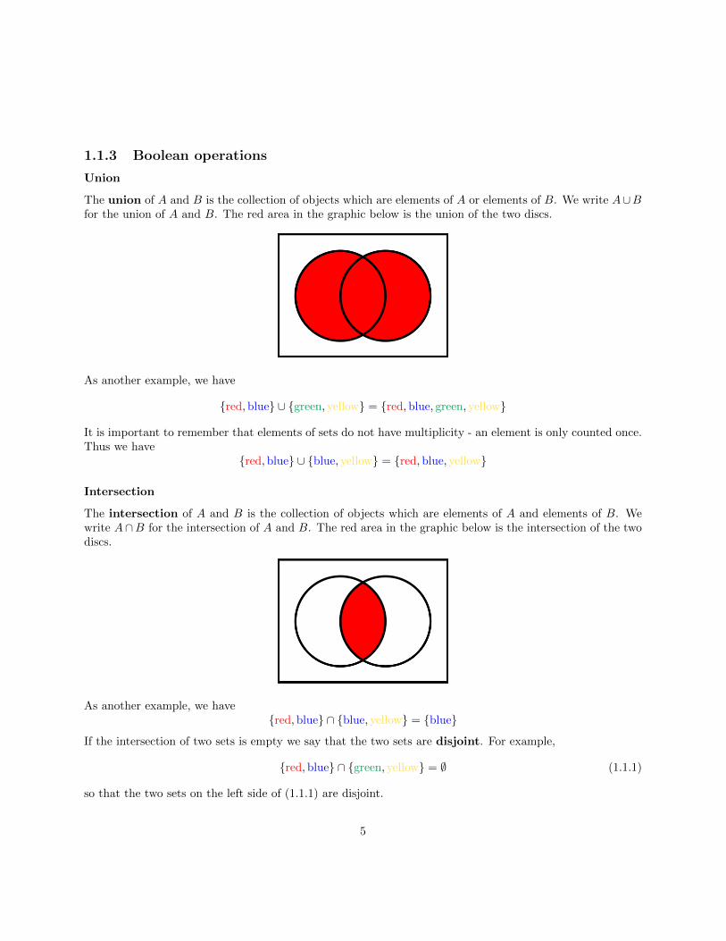
1.1.3 Boolean operations

Union

The union of A and B is the collection of objects which are elements of A or elements of B. We write A∪Bfor the union of A and B. The red area in the graphic below is the union of the two discs.

As another example, we have

{red,blue} ∪ {green, yellow} = {red,blue, green, yellow}

It is important to remember that elements of sets do not have multiplicity - an element is only counted once.Thus we have

{red,blue} ∪ {blue, yellow} = {red,blue, yellow}

Intersection

The intersection of A and B is the collection of objects which are elements of A and elements of B. Wewrite A∩B for the intersection of A and B. The red area in the graphic below is the intersection of the twodiscs.

As another example, we have{red,blue} ∩ {blue, yellow} = {blue}

If the intersection of two sets is empty we say that the two sets are disjoint. For example,

{red,blue} ∩ {green, yellow} = ∅ (1.1.1)

so that the two sets on the left side of (1.1.1) are disjoint.

5

Difference

The difference A minus B is the collection of objects which are elements of A but not elements of B. Wewrite A \B for the difference A minus B. The red area in the graphic below is the right disc minus the leftdisc.

As another example, we have{red,blue} \ {blue, yellow} = {red}

1.2 Functions

1.2.1 Basic information

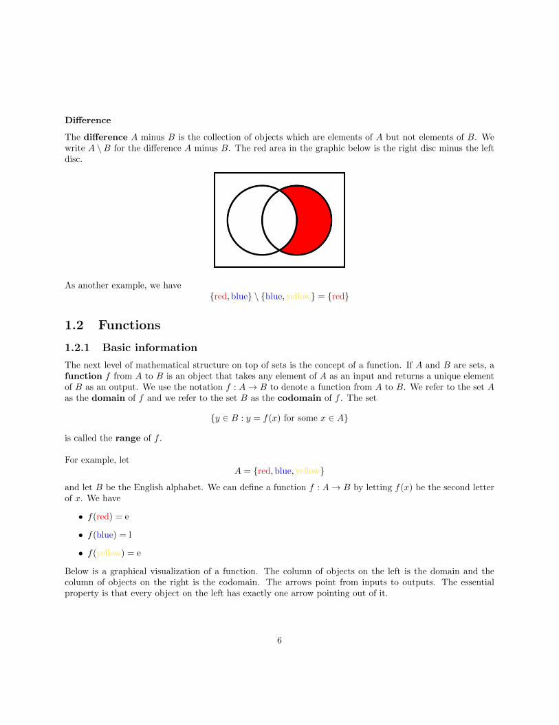
The next level of mathematical structure on top of sets is the concept of a function. If A and B are sets, afunction f from A to B is an object that takes any element of A as an input and returns a unique elementof B as an output. We use the notation f : A→ B to denote a function from A to B. We refer to the set Aas the domain of f and we refer to the set B as the codomain of f . The set

{y ∈ B : y = f(x) for some x ∈ A}

is called the range of f .

For example, letA = {red,blue, yellow}

and let B be the English alphabet. We can define a function f : A→ B by letting f(x) be the second letterof x. We have

• f(red) = e

• f(blue) = l

• f(yellow) = e

Below is a graphical visualization of a function. The column of objects on the left is the domain and thecolumn of objects on the right is the codomain. The arrows point from inputs to outputs. The essentialproperty is that every object on the left has exactly one arrow pointing out of it.

6

•

∗

?

◦

◦

•

?

∗

1.2.2 Three essential properties

Injectivity

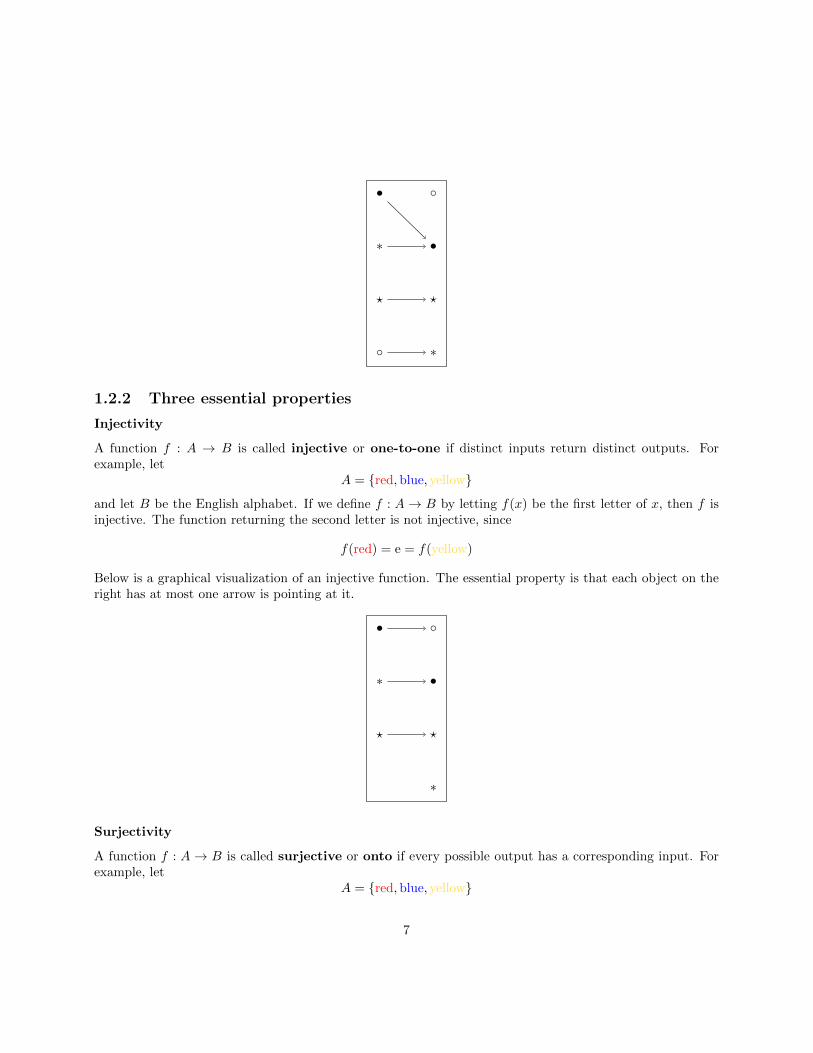
A function f : A → B is called injective or one-to-one if distinct inputs return distinct outputs. Forexample, let

A = {red,blue, yellow}

and let B be the English alphabet. If we define f : A→ B by letting f(x) be the first letter of x, then f isinjective. The function returning the second letter is not injective, since

f(red) = e = f(yellow)

Below is a graphical visualization of an injective function. The essential property is that each object on theright has at most one arrow is pointing at it.

•

∗

?

◦

•

?

∗

Surjectivity

A function f : A → B is called surjective or onto if every possible output has a corresponding input. Forexample, let

A = {red,blue, yellow}

7

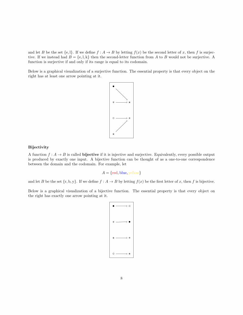
and let B be the set {e, l}. If we define f : A→ B by letting f(x) be the second letter of x, then f is surjec-tive. If we instead had B = {e, l, k} then the second-letter function from A to B would not be surjective. Afunction is surjective if and only if its range is equal to its codomain.

Below is a graphical visualization of a surjective function. The essential property is that every object on theright has at least one arrow pointing at it.

•

∗ ?

◦

?

∗

Bijectivity

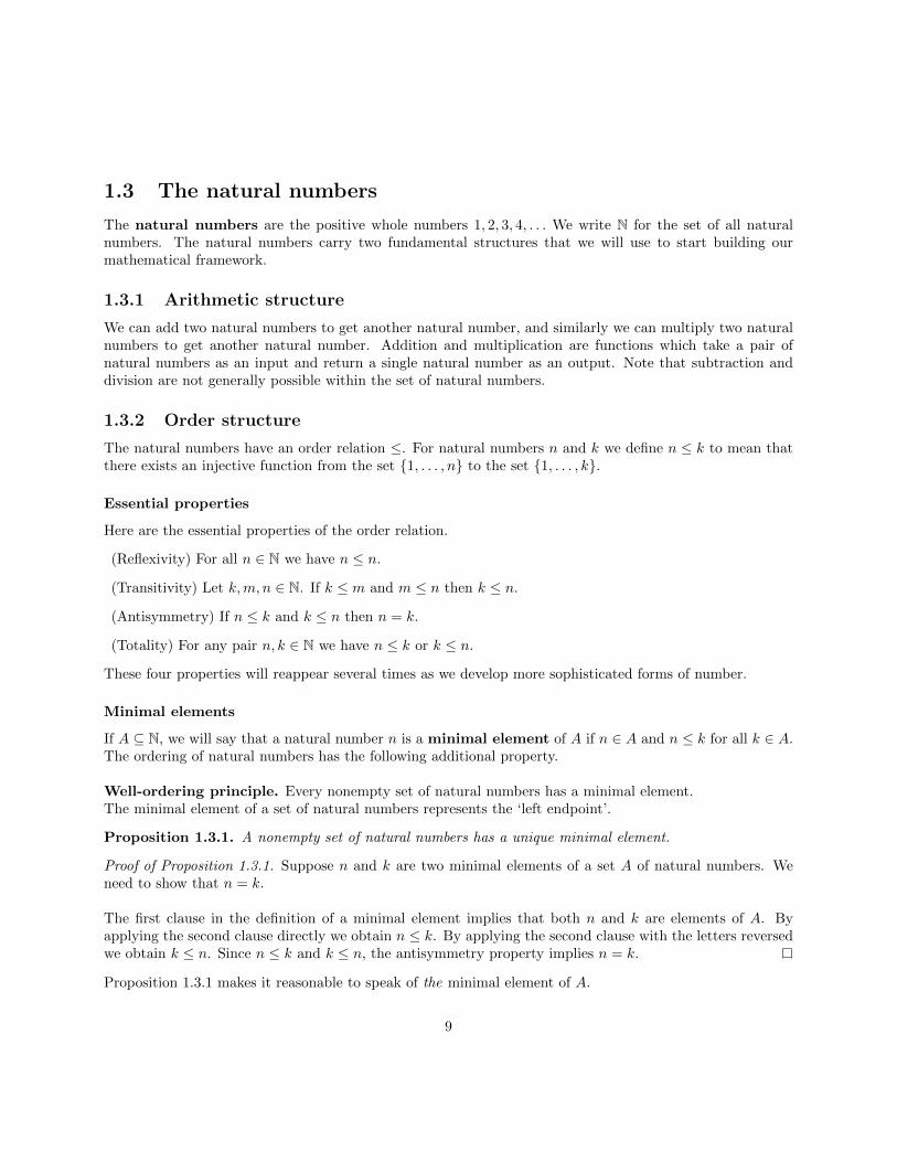
A function f : A→ B is called bijective if it is injective and surjective. Equivalently, every possible outputis produced by exactly one input. A bijective function can be thought of as a one-to-one correspondencebetween the domain and the codomain. For example, let

A = {red,blue, yellow}

and let B be the set {r,b, y}. If we define f : A→ B by letting f(x) be the first letter of x, then f is bijective.

Below is a graphical visualization of a bijective function. The essential property is that every object onthe right has exactly one arrow pointing at it.

•

∗

?

◦

•

∗

◦ ?

8

1.3 The natural numbers

The natural numbers are the positive whole numbers 1, 2, 3, 4, . . . We write N for the set of all naturalnumbers. The natural numbers carry two fundamental structures that we will use to start building ourmathematical framework.

1.3.1 Arithmetic structure

We can add two natural numbers to get another natural number, and similarly we can multiply two naturalnumbers to get another natural number. Addition and multiplication are functions which take a pair ofnatural numbers as an input and return a single natural number as an output. Note that subtraction anddivision are not generally possible within the set of natural numbers.

1.3.2 Order structure

The natural numbers have an order relation ≤. For natural numbers n and k we define n ≤ k to mean thatthere exists an injective function from the set {1, . . . , n} to the set {1, . . . , k}.

Essential properties

Here are the essential properties of the order relation.

(Reflexivity) For all n ∈ N we have n ≤ n.

(Transitivity) Let k,m, n ∈ N. If k ≤ m and m ≤ n then k ≤ n.

(Antisymmetry) If n ≤ k and k ≤ n then n = k.

(Totality) For any pair n, k ∈ N we have n ≤ k or k ≤ n.

These four properties will reappear several times as we develop more sophisticated forms of number.

Minimal elements

If A ⊆ N, we will say that a natural number n is a minimal element of A if n ∈ A and n ≤ k for all k ∈ A.The ordering of natural numbers has the following additional property.

Well-ordering principle. Every nonempty set of natural numbers has a minimal element.The minimal element of a set of natural numbers represents the ‘left endpoint’.

Proposition 1.3.1. A nonempty set of natural numbers has a unique minimal element.

Proof of Proposition 1.3.1. Suppose n and k are two minimal elements of a set A of natural numbers. Weneed to show that n = k.

The first clause in the definition of a minimal element implies that both n and k are elements of A. Byapplying the second clause directly we obtain n ≤ k. By applying the second clause with the letters reversedwe obtain k ≤ n. Since n ≤ k and k ≤ n, the antisymmetry property implies n = k.

Proposition 1.3.1 makes it reasonable to speak of the minimal element of A.

9

1.4 Finite sets

We will say that a set A is finite if A is empty or if there exists a natural number n and a bijection betweenA and the set {1, . . . , n}. For example, let

A = {red,blue, yellow}

This set is finite. We can define a bijection f : A→ {1, 2, 3} by setting

• f(red) = 1

• f(blue) = 2

• f(yellow) = 3.

Finite sets are those which can enumerated with a terminating process.

Proposition 1.4.1. For any nonempty finite set A, there is a unique natural number n such that there existsa bijection from A to {1, . . . , n}.

Proof of Proposition 1.4.1. Suppose that n and k are natural numbers such that there exist bijectionsf : A→ {1, . . . , n} and g : A→ {1, . . . , k}. We need to show n = k.

The first idea is that a bijection can be inverted. In other words, if h : B → C is a bijection, then there existsa bijection h−1 : C → B such that h−1(h(x)) = x for all x ∈ B. The second idea is that the composition oftwo bijections is a bijection.

Therefore g◦f−1 is a bijection from {1, . . . , n} to {1, . . . , k}. Here g◦f−1 is given by (g◦f−1)(m) = g(f−1(m)).

The existence of this bijection implies that n ≤ k and the fact that its inverse is a bijection implies k ≤ n.Therefore antisymmetry implies n = k.

The unique natural number n such that there exists a bijection between A and {1, . . . , n} is called the size orcardinality of A. We denote this by writing |A| = n. The empty set is the unique set with cardinality zero.

One can check that if A and B are finite sets then the following are equivalent.

• |A| ≤ |B|

• There exists an injective function from A to B.

• There exists a surjective function from B to A.

1.5 Infinite sets

We say a set is infinite if it is not finite.

Proposition 1.5.1. The whole set of natural numbers is infinite.

10

Proof of Proposition 1.5.1. We use the technique of proof by contradiction. Suppose toward a contradictionthat N were finite. Then there would exist a natural number n and a bijection f : N→ {1, . . . , n}.

Let f : {1, . . . , n + 1} → {1, . . . , n} be defined by f(k) = f(k) for all k ∈ {1, . . . , n + 1}. This processof restricting the domain of a bijective function always produces an injective function. Since f is an injectivefunction from {1, . . . , n + 1} to {1, . . . , n}, we obtain n + 1 ≤ n. This is obviously false. Thus, our initialhypothesis must also be false and so N is infinite.

A counterintuitive property of infinite sets is that there can exist an injective function from an infinite set toa proper subset of itself. For example, the function f : N→ {2, 3, 4, . . . , } given by f(n) = n+ 1 is injective,but its range misses the number 1.

Let E be the set of even natural numbers. The function f : N → E given by f(n) = 2n is also injec-tive, but its range misses the whole infinite set of odd numbers.

The way to interpret this is that an infinite set can have the same size as a proper subset of itself.

1.6 Mathematical induction

1.6.1 The method

Mathematical induction is a method to prove statements about the natural numbers. Proofs by mathematicalinduction can be good practice for developing mathematical writing skills, as they are highly formalized andin some sense are intermediate between computations and more advanced proofs.

Let P (n) be a property of a natural number n. For example, P (n) could be the statement that n ≤ n2.The goal of a proof by induction is to prove that P (n) is true for all n ∈ N. The paradigm consists of two steps.

Initial step. In the initial step, one checks that P (1) is true. This step is usually easy, but it is im-portant to remember to perform it.

Inductive step. In the inductive step, one assumes that P (n) holds for some natural number n. Thenone uses this assumption to prove that P (n+ 1) holds.

If both steps are verified, one concludes that P (n) is true for all n ∈ N.

1.6.2 Justification from well-ordering

Recall the well-ordering principle for the natural numbers.

Well-ordering principle. Every nonempty set of natural numbers has a minimal element.

We can use the well-ordering principle to establish that the method of mathematical induction is valid.

Suppose that we have completed both steps for a given property P and let A be the set of natural numbersfor which P fails. In order to justify the conclusion, we need to show that A is empty.

11

Suppose toward a contradiction that A were nonempty. Then by the well-ordering principle, A would havea minimal element a.

The initial step implies that P (1) is true, so we must have a > 1. Therefore a− 1 is also a natural number.Since a is the least number for which P fails, it must be the case that P holds for a− 1.

The inductive step says that if P holds for some number n, then P also holds for n + 1. Therefore Pholds for a = (a− 1) + 1. This contradicts the hypothesis that a ∈ A.

1.6.3 First example

We now give an example of a proof by mathematical induction.

Proposition 1.6.1. Let P (n) be following statement:

1 + 2 + 3 + · · ·+ (n− 1) + n =n(n+ 1)

2

Then P (n) holds for all n ∈ N.

Proof of Proposition 1.6.1. We proceed to follow the method of induction.

Initial step. We check that P (1) holds:

1 =1(1 + 1)

2.

Inductive step. Here we assume that P (n) holds for a natural number n. Explicitly, this means we assumethat

1 + 2 + 3 + · · ·+ (n− 1) + n =n(n+ 1)

2.

We need to show that P (n+ 1) holds. Explicitly, this means we need to show that

1 + 2 + 3 + · · ·+ (n− 1) + n+ (n+ 1) =(n+ 1)(n+ 2)

2.

We compute

1 + 2 + 3 + · · ·+ (n− 1) + n+ (n+ 1) = (1 + 2 + 3 + · · ·+ (n− 1) + n) + n+ 1 (1.6.1)

=n(n+ 1)

2+ n+ 1 (1.6.2)

=n2 + n

2+

2n+ 2

2

=n2 + 3n+ 2

2

=(n+ 1)(n+ 2)

2

Here we used the inductive assumption to pass from (1.6.1) to (1.6.2).

12

1.6.4 Delayed induction

Mathematical induction also works if we start from some number m greater than 1. In this case, for ourinitial step we check that P (m) is true. In the inductive step we assume that P (n) holds for some n ≥ mand we need to show that P (n+ 1) holds. After both of these steps have been verified, we conclude that Pholds for all numbers greater than or equal to m.

We now consider an example of this ‘delayed’ induction. Recall the notion of a factorial:

n! = 1 · 2 · 3 · · · (n− 2) · (n− 1) · n.

Proposition 1.6.2. Let P (n) be the statement n! ≥ 2n. Then P (n) holds for all n ≥ 4

The statement in Proposition 1.6.2 is not true for every natural number, since 1! = 1 < 2 = 21.

Proof of Proposition 1.6.2. We proceed with induction starting from the number 4.

Initial step. We check P (4):4! = 2 · 3 · 4 = 24 ≥ 16 = 24.

Inductive step. We assume that P (n) is true, that is we assume n! ≥ 2n. We compute

(n+ 1)! = n! · (n+ 1) (1.6.3)

≥ 2n · (n+ 1) (1.6.4)

≥ 2n · 2= 2n+1.

Here we used the inductive hypothesis to pass from (1.6.3) to (1.6.4).

1.7 Integers and rational numbers

1.7.1 Integers

We observed that subtraction and division are not generally possible within the natural numbers. This isproblematic, as in order to develop calculus we will certainly need these operations.

We can enable subtraction by adjoining zero and the negatives of natural numbers. This results in theintegers

. . . ,−3,−2,−1, 0, 1, 2, 3, . . .

We use the symbol Z for the set of integers.

Like the natural numbers, the integers have an order structure. However, the well-ordering principle fails forthe integers: the whole set of integers is nonempty and it has no minimal element. Nevertheless, somethingclose to the well-ordering principle holds.

Given a set A of integers, a lower bound for A is an integer n such that n ≤ k for all k ∈ A. Wesay that n is a greatest lower bound for A if n is a lower bound for A and any other lower bound m for

13

A satisfies m ≤ n. One can check that in the context of the natural numbers, a greatest lower bound is thesame thing as a minimal element.

Greatest lower bound principle for Z. If a nonempty set of integers has a lower bound, then it has agreatest lower bound.

We can establish that the greatest lower bound of a set of integers is unique if it exists using the sameargument we used to show that the minimal element of a set of natural numbers is unique.

1.7.2 Countably infinite sets

If there exists a bijection between a set A and the natural numbers, we say that A is countably infinite. Wesay that A is countable if it is countably infinite or finite.

Intuitively, countable sets are no larger than the natural numbers.

The set of integers is countable. For example, we can define a bijection f : N→ Z by

f(n) =

n− 1

2if n is odd

−n2

if n is even

1.7.3 Rational numbers

Basic information

We can enable division by considering the rational numbers. A rational number is an expression of the formnk where n is an integer and k is a nonzero integer. We make the convention that two such expressions n

k andml denote the same rational number if nl = mk. We use the symbol Q to denote the set of rational numbers.

Avoiding division by zero

The qualification that k is nonzero in the characterization of rational numbers reflects the mathematicalconsensus that division by zero is not advisable. Let us try to understand why this consensus exists.

Suppose that we could assign a numerical value to the expression 10 . Then we should certainly have 0 · 10 = 1.

On the other hand, basic considerations about rational numbers entail that 0 ·x = 0 for all x ∈ Q. Combiningthe last two expressions, we see that if we allow division by zero by then we are forced to conclude that 0 = 1.Following the principle that 0 · x = 0 for all x, we obtain the conclusion that 0 = 0 · x = 1 · x = x for allx ∈ Q.

Thus the only way to make sense of division by zero is to conclude that zero is the only rational num-ber that exists. Since this conclusion is obviously inconsistent with the fundamental utility of numbers, weare compelled to avoid division by zero in all circumstances.

14

Artihmetic of rational numbers

We can add and multiply rational numbers in the usual way:

n

k+m

l=nl + km

kln

k· ml

=nm

kl

For the purposes of this text, we take the arithmetic of rational numbers as understood.

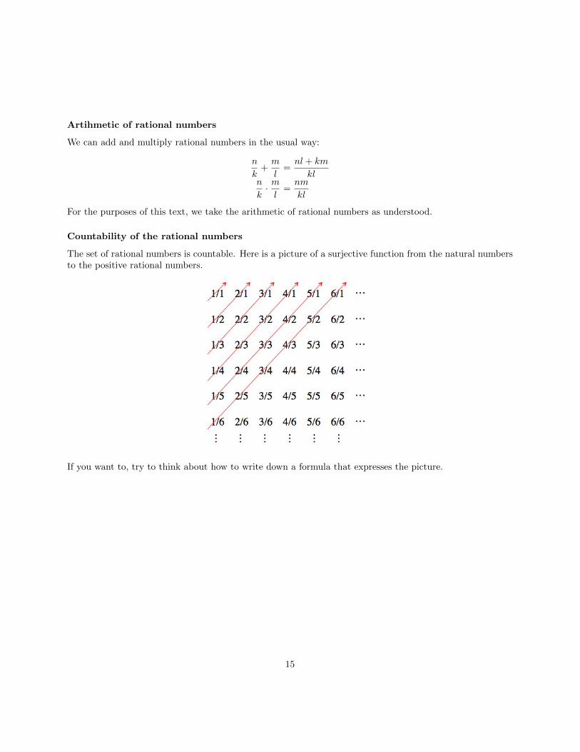
Countability of the rational numbers

The set of rational numbers is countable. Here is a picture of a surjective function from the natural numbersto the positive rational numbers.

If you want to, try to think about how to write down a formula that expresses the picture.

15

Chapter 2

The real number system

2.1 The real numbers

2.1.1 Motivation

The rational numbers are very nice arithmetically - one has all four basic operations. However, they are stillnot rich enough to develop calculus.

The reason is that the greatest lower bound property is essential for calculus, and it fails badly for therational numbers. For example, consider the set

{q ∈ Q : q ≥ 0 and q2 ≥ 2}.

This set has a lower bound of 0 by construction. However, it has no greatest lower bound in the rationalnumbers. The greatest lower bound ‘should’ be

√2, but this is not a rational number.

In order to rectify this situation, we will need to extend our system to the real numbers. Intuitively, the realnumbers are designed to fill in all the infinitesimal holes in the rational numbers. It is possible to constructthe real numbers directly from the rational numbers, but instead we will take an axiomatic approach.

We write R for the set of real numbers. We will now proceed to list out fourteen axioms which charac-terize the real number system. These axioms will be the basis for all the work we do in the rest of thetext.

2.1.2 Fourteen axioms

Addition is an abelian group

R is equipped with a binary operation called addition, which takes a pair of real numbers and returns a singlereal number. We denote addition with the infix notation +. The first four axioms describe the behavior ofaddition.

• Axiom 1 (associativity of addition) For all x, y, z ∈ R we have (x+ y) + z = x+ (y + z).

16

• Axiom 2 (existence of additive identity) There exists a distinguished element 0 ∈ R such that 0+x = xfor all x ∈ R.

• Axiom 3 (existence of additive inverses) For every x ∈ R there exists a corresponding element −x suchthat x+ (−x) = 0.

• Axiom 4 (commutativity of addition) For all x, y ∈ R we have x+ y = y + x.

In algebraic terms, Axioms 1 - 3 assert that the real numbers with addition form an object called a group.When we add Axiom 4, the object is called an abelian group.

Axiom 1 belongs to the unusual class of mathematical statements which are so obvious to the intuitionthat their actual content is somewhat opaque. This axiom is necessary because we stipulated that additionwas a binary operation, so a priori it does not make sense to add three real numbers. Axiom 1 asserts theequivalence of two plausible methods for decomposing the sum of three real numbers into iterated binarysums. Thus we can unambiguously speak of the sum of three real numbers. Repeated applications of Axiom1 extend this to the sum of any finite list of real numbers. Even in our first axiomatic proofs below inSubsection 2.1.4, we will use Axiom 1 implicitly by writing expressions such as x+ y + z.

If x and y are real numbers, we will typically write x − y for x + (−y). If x1, . . . , xn is a finite list ofreal numbers we will typically write

∑nk=1 xk for the sum x1 + x2 + · · · + xn−1 + xn. Observe that in this

notation the variable k is bound by the sum. Thus we must avoid using the variable k for another purposein an expression involving the notation

∑nk=1 xk.

Multiplication without zero is an abelian group

R is equipped with a second binary operation called multiplication, which we denote by · or simply byjuxtaposition. The next four axioms describe the behavior of multiplication.

• Axiom 5 (associativity of multiplication) For all x, y, z ∈ R we have (x · y) · z = x · (y · z).

• Axiom 6 (existence of multiplicative identity) There exists a distinguished element 1 ∈ R such that1 · x = x for all x ∈ R.

• Axiom 7 (existence of multiplicative inverses) For each x ∈ R such that x 6= 0 there exists a corre-sponding element x−1 such that x · x−1 = 1.

• Axiom 8 (commutativity of multiplication) For all x, y ∈ R we have x · y = y · x.

These axioms assert that the nonzero real numbers form an abelian group under multiplication. As withAxiom 1 for addition, Axiom 5 allows us to multiply any finite list of real numbers.

Later in the text we will develop the theory of exponentiation, in which the association x 7→ x−1 describedby Axiom 7 will be generalized to a family of operations where the superscript −1 can replaced by other realnumbers. For the purposes of the axiomatization we regard the superscript −1 as purely a formal symbolwhich can be manipulated in accordance with Axiom 7.

If x and y are real numbers, we will typically write xy for x · y. For n ∈ N we will typically write xn

for x · x · · ·x · x, where there are n terms in the product. If y is nonzero we will typically write xy for x · y−1.

17

In particular, in accordance with Axiom 6 we will write 1y for y−1 = 1 · y−1. If x1, . . . , xn is a finite list of

real numbers, we will typically write∏nk=1 xk for the product x1 · x2 · · ·xn−1 · xn.

Inherent in Axiom 7 is that division by zero is not advisable.

Multiplication distributes over addition

The next axiom describes how addition and multiplication interact with each other.

• Axiom 9 (distributivity of multiplication over addition) For all x, y, z ∈ R we have x · (y + z) =(x · y) + (x · z).

Nondegeneracy

• Axiom 10 (nondegeneracy) The numbers 0 and 1 are distinct.

Axiom 10 is necessary for the simple reason that explicitly stipulating 0 6= 1 is the only way to rule out theundesirable possibility that 0 = 1. In accordance with the discussion in Subsection 1.7.3, we see that Axiom10 is intimately connected with the avoidance of division by zero.

Taken together, Axioms 1 - 10 describe the properties of an algebraic object called a field.

Order structure

The real numbers have a special subset called the positive numbers. We denote the positive numbers by P.The set P has the following properties.

• Axiom 11 (stability of P under addition) If x, y ∈ P then x+ y ∈ P.

• Axiom 12 (stability of P under multiplication) If x, y ∈ P then x · y ∈ P.

• Axiom 13 (trichotomy property) For any x ∈ R exactly one of the following conditions holds:

(x is positive) We have x ∈ P.

(x is zero) We have x = 0.

(x is negative) We have −x ∈ P.

We can use P to define an ordering on the real numbers. We stipulate that x < y if and only if y − x ∈ P.We also use the notation x ≤ y to mean x < y or x = y.

By applying Axiom 3 to x = 0 we see that 0 + (−0) = 0. By applying Axiom 2 to the previous equal-ity we see that −0 = 0. Therefore if x ∈ P we can apply Axiom 2 to see that x − 0 = x + 0 = x ∈ P. Thisjustifies the more common notation x > 0 for the assertion that x ∈ P.

18

Completeness

Axioms 1 - 13 describe an object called an ordered field. All of the axioms listed so far hold for the rationalnumbers, so the rational numbers are also an ordered field. We now introduce the final axiom, which distin-guishes the real numbers from the rational numbers and which makes calculus possible.

If A is a nonempty set of real numbers, we say that x ∈ R is a lower bound for A if x ≤ y for ally ∈ A. We say that x is a greatest lower bound for A if x is a lower bound for A and if every lower boundz for A satisfies z ≤ x. This is the same definition we made for our previous sets of numbers.

• Axiom 14 (completeness of R) If a nonempty set of real numbers has a lower bound, then it has agreatest lower bound.

If A is a nonempty set of real numbers with an upper bound, we can apply Axiom 14 to the set {−x : x ∈ A}to see that the set A has a least upper bound. We will use the word infimum to refer to the greatest lowerbound and the word supremum to refer to the least upper bound. We will typically write inf A and supAfor the infimum and supremum of A respectively.

Axioms 1 - 14 assert that the real numbers form a complete ordered field. It is possible to prove thatthere is exactly one complete ordered field, in the sense that any two structures satisfying Axioms 1 - 14are essentially the same. This uniqueness allows us to think of the set of real numbers as a single canonicalobject, in the same way that we think of the natural numbers.

2.1.3 Embedding Q in RThere are canonical embeddings of all our previous sets of numbers into R. Axiom 6 gave us the existenceof the real number 1. We can identify the real number 1 with the natural number 1. More generally, wecan identify the natural number n with the real number 1+1+ · · ·+1+1, where there are n terms in the sum.

Given the identification of N with a subset of R, Axiom 3 provides us with a way to embed Z in R. Specifi-cally, for a natural number n we identify the integer −n with the additive inverse of the real number n.

Finally, Axiom 7 provides us with a way to embed Q in R. Specifically, we for an integer n and a nonzerointeger k we identify the rational number n

k with the real number n · k−1.

2.1.4 Examples of axiomatic proofs

In Subsection 2.1.4 we will give several examples of how to use the axioms to prove statements about thereal numbers. These proofs will justify each step by explicitly citing an axiom. They will use only Axioms 1- 13. In Subsection 2.1.5 below we will give an example of a proof using the more subtle Axiom 14.

Proposition 2.1.1 (cancellative law for addition). Suppose that x, y and z are real numbers such thatx+ y = x+ z. Then y = z.

Proof of Proposition 2.1.1. Let x, y and z be as in the statement of Proposition 2.1.1.

• Axiom 3 provides us with the real number −x. From the hypothesis x+ y = x+ z we obtain

−x+ x+ y = −x+ x+ z (2.1.1)

19

• By Axiom 4, we have −x+ x = x+ (−x) so that from (2.1.1) we obtain

x+ (−x) + y = x+ (−x) + z (2.1.2)

• By applying Axiom 3 to both sides of (2.1.2) we obtain

0 + y = 0 + z (2.1.3)

• By applying Axiom 2 to both sides of (2.1.3) we obtain y = z as required.

Proposition 2.1.2 (translation preserves inequalities). Let x, y and z be real numbers. If x < y thenx+ z < y + z.

Proof of Proposition 2.1.2. Let x, y and z be as in the statement of Proposition 2.1.2.

• By definition, the hypothesis x < y means y − x ∈ P.

• By Axiom 2, we have y − x+ 0 = y − x, so that y − x+ 0 ∈ P.

• By Axiom 3, we have y − x+ 0 = y − x+ z − z, so that y − x+ z − z ∈ P.

• By Axiom 4, we have y − x+ z − z = y + z − x− z, so that

y + z − x− z ∈ P (2.1.4)

• We claim that−x− z = −(x+ z) (2.1.5)

Indeed, by combining Axioms 2, 3 and 4 we have

x+ z − x− z = x− x+ z − z = 0 + 0 = 0 (2.1.6)

By Axiom 3 we havex+ z − (x+ z) = 0 (2.1.7)

The claim (2.1.5) follows by applying Lemma 2.1.1 to (2.1.6) and (2.1.7).

• By combining (2.1.4) and (2.1.5) we obtain y+ z− (x+ z) ∈ P. By definition, this means x+ z < y+ zas required.

Corollary 2.1.1. Let x be a real number and let z be a positive number. Then x < x+ z.

Proof of Corollary 2.1.1. Let x and z be as in the statement of Corollary 2.1.1. Since z > 0, Lemma 2.1.2implies x+ z > x+ 0. By Axiom 2 we have x+ 0 = x so that x+ z > x as required.

Theorem 2.1.2 (an ε of room). Suppose that x and y are real numbers such that y ≤ x+ ε for every positivenumber ε. Then y ≤ x.

20

Proof of Theorem 2.1.2. Suppose toward a contradiction that there exist real numbers x and y is as in thestatement of Theorem 2.1.2, but such that the conclusion of Theorem 2.1.2 fails for x and y. By Axiom 13,we see that if y ≤ x fails then we have y > x.

• By Axioms 2, 3 and 4 we havex+ y − x = y (2.1.8)

• By Axioms 6 and 9 we have

x+ y − x = x+ 1 · (y − x) = x+

(1

2+

1

2

)(y − x) = x+

1

2(y − x) +

1

2(y − x) (2.1.9)

• By combining (2.1.8) and (2.1.9) we obtain

y = x+1

2(y − x) +

1

2(y − x) (2.1.10)

• The hypothesis that y > x implies y−x ∈ P. From our understanding of rational numbers, we see that12 ∈ P. Therefore Axiom 12 implies 1

2 (y − x) ∈ P.

• By applying Corollary 2.1.1 to (2.1.10) we obtain

y > x+1

2(y − x) (2.1.11)

• Since 12 (y − x) ∈ P, the hypothesis that y ≤ x+ ε for all ε ∈ P implies

y ≤ x+1

2(y − x) (2.1.12)

• The combination of (2.1.11) and (2.1.12) is inconsistent with the exclusivity of the trichotomy in Axiom13. Thus we have obtain a contradiction and the proof of Theorem 2.1.2 is complete.

The proofs of Propositions 2.1.1 and 2.1.2 and of Theorem 2.1.2 have been written so that we can verifythe arguments using the axioms in an essentially mechanical way. There is an extensive project to rewriteall mathematical literature in an analogous style so as to enable verification by computer. However, it isinfeasible for human beings to think deeply about mathematics in this fashion. In the remainder of the text,we will write proofs to optimize human understanding rather than mechanical verification.

2.1.5 Existence of√2

Recall that our original motivation for developing the set of real numbers was that the set

{q ∈ Q : q ≥ 0, q2 ≥ 2}

had no greatest lower bound in the rational numbers. Since we are now working with real numbers, we willenlarge this set by letting

A = {x ∈ R : x ≥ 0, x2 ≥ 2}.By Axiom 14, the set A has a greatest lower bound in the real numbers. It follows from the definition thatthere is at most one greatest lower bound for any set. Let s be the unique greatest lower bound of A.

21

Theorem 2.1.3. We have s2 = 2.

We can interpret Theorem 2.1.3 as saying that Axiom 14 has provided us with the existence of the irrationalreal number

√2.

Proof of Theorem 2.1.3. We proceed by ruling out each of the possibilities s2 > 2 and s2 < 2. If we do this,we will know that s2 − 2 is neither positive nor negative. Then Axiom 13 will imply that s2 − 2 = 0.

Case 1. In this case we assume s2 > 2 and endeavor to obtain a contradiction. The way we will do this isby finding an element x ∈ A such that x < s. This will contradict the hypothesis that s is a lower bound of A.

The number 1 is a lower bound for A since x2 ≥ 2 and x ≥ 0 imply x ≥ 1. Hence the assumptionthat s is the greatest lower bound for A implies s ≥ 1. Therefore 2s ≥ 2 > 0.

Our hypothesis that s2 > 2 implies that s2 − 2 > 0. Therefore we have

s2 − 2

2s> 0

Lemma 2.1.2 implies that there exists ε > 0 such that

s2 − 2

2s> ε

or equivalentlys2 − 2 > 2εs (2.1.13)

Consider the number s− ε. We claim that s− ε ∈ A. Since s− ε < s, this will violate the hypothesis that sis a lower bound for A.

In order to show s− ε ∈ A we need to show that (s− ε)2 ≥ 2. We compute:

(s− ε)2 = s2 − 2εs+ ε2

> s2 − 2εs (2.1.14)

> s2 − (s2 − 2) (2.1.15)

= 2

Here in passing from (2.1.14) to (2.1.15) we used applied (2.1.13) to increase the size of the subtracted termand thereby decrease the overall size of the quantity. This completes the analysis of Case 1.

Case 2. In the case we assume that s2 < 2 and again endeavor to obtain a contradiction. The waywe will do this is by finding a real number x > s such that x is a lower bound for A. This will contradict thehypothesis that s is the greatest lower bound of A.

Our assumption implies that 2− s2 > 0. Therefore we can find a number ε > 0 such that

ε <2− s2

2s+ 1

22

Equivalently, we haveε(2s+ 1) < 2− s2. (2.1.16)

We may assume without loss of generality that ε < 1. We claim that x = s + ε is a lower bound for A. Toverify this, let y ∈ A, so that we have y2 ≥ 2. We must show that s+ ε ≤ y.

We compute:

(s+ ε)2 = s2 + 2εs+ ε2 (2.1.17)

< s2 + 2εs+ ε (2.1.18)

= s2 + ε(2s+ 1) (2.1.19)

< s2 + 2− s2 (2.1.20)

= 2

≤ y2

Here in passing from (2.1.17) to (2.1.18) we used the assumption that ε < 1 to conclude ε2 < ε, and in passingfrom (2.1.19) to (2.1.20) we applied (2.1.16).

We have shown that (s+ ε)2 ≤ y2. Therefore

0 ≤ y2 − (s+ ε)2 = (y − s− ε)(y + s+ ε).

Dividing by the positive number y + s+ ε we obtain 0 ≤ y − s− ε so that s+ ε ≤ y.

Since y was an arbitrary element of A, we see that s + ε is a lower bound for A. This contradicts thehypothesis that s was the greatest lower bound for A, completing the analysis of Case 2 and thereby com-pleting the proof of Theorem 2.1.3.

2.2 Uncountable sets

Recall that a set A is said to be countably infinite if there exists a bijection between A and the set N ofnatural numbers. A set is countable if it is finite or countably infinite. Intuitively, countable sets are nolarger than the natural numbers. It is clear that a subset of a countable set is again countable. We saw thatthe rational numbers are countable, despite being a proper superset of the natural numbers.

We will say that a set is uncountable if it is not countable. Uncountable sets are infinite in a largersense than countable sets - they cannot be enumerated with natural numbers. It is not obvious that un-countable sets exist. We will establish below in Theorem 2.2.1 that they do. This fact was considered verysurprising when it was discovered in the late 19th century. Most people have a misguided initial intuitionthat all infinities are equally large.

2.2.1 Uncountability of the set of binary sequences

An infinite binary sequence is a function α from N to the set {0, 1}. We can visualize an infinite binarysequence as a string of zeroes and ones which goes on indefinitely to the right, where the bit α(n) appears inthe nth position. We denote the set of all infinite binary sequences by {0, 1}N.

23

Theorem 2.2.1. There exists an uncountable set. More specifically, the set {0, 1}N is uncountable.

Proof of Theorem 2.2.1. Suppose toward a contradiction that {0, 1}N is countable. This means there existsa bijection f from N to {0, 1}N. We will use the notation αn for f(n). Thus for each natural number n wehave an infinite binary sequence αn. Our hypothesis is that the list α1, α2, α3, . . . enumerates all the possibleinfinite binary sequences. We will obtain a contradiction by exhibiting an infinite binary sequence β whichis not part of this enumerated list.

The technique for constructing β is referred to as diagonalization. Intuitively, we design β such that itdiffers from αn in the nth bit. More precisely, define

β(n) =

{0 if αn(n) = 1

1 if αn(n) = 0

For every n ∈ N we have β(n) 6= αn(n) and therefore β 6= αn. Since n was arbitrary, we conclude that β isnot part of our enumerated list. This completes the proof of Theorem 2.2.1.

The proof of Theorem 2.2.1 is quite brief, but the underlying idea can be vastly generalized. An exampleof such a generalization is the existence of mathematical problems which cannot be completely solved bya computer program. For more information about such generalizations, research the unsolvability of thehalting problem.

2.2.2 Uncountability of the real numbers

We will use Theorem 2.2.1 to establish that R is uncountable by exhibiting an injective function from {0, 1}Nto R. This means that the infinite size of the set of new quantities that we introduced when completing therational numbers is larger than the infinite size of the rational numbers themselves.

Two lemmas on geometric sums

Before we prove that R is uncountable, we will establish a formula for a certain type of sum of real numbersthat will used in mapping {0, 1}N to R.

A geometric progression is a sequence x1, x2, x3, . . . of positive real numbers such that the ratio xn+1

xn

of successive terms is constant. A geometric progression has the form a, ab, ab2, ab3, . . . for positive numbersa = x1 and b = xn+1

xn.

Lemma 2.2.1 (Formula for geometric sums). For any positive number b different from 1 we have

n∑k=0

bk =1− bn+1

1− b

Proof. We compute

(1− b)n∑k=0

bk =

n∑k=0

bk − bn∑k=0

bk

24

=

n∑k=0

bk −n∑k=0

bk+1 (2.2.1)

= 1− bn+1 (2.2.2)

Here, (2.2.2) follows from (2.2.1) since the terms b, b2, . . . , bn−1, bn appear in both sums in (2.2.1) and henceare cancelled.

The next lemma will be the key to our proof that R is uncountable.

Lemma 2.2.2. For any m,n ∈ N we have

n∑k=1

1

10m+k≤ 1

9 · 10m

Proof. We have

n∑k=1

1

10m+k=

1

10m+1

n−1∑k=0

1

10k(2.2.3)

=1

10m+1

1− 10−n

1− 10−1(2.2.4)

=1

10m+1

10(1− 10−n)

9(2.2.5)

≤ 1

10m+1

10

9(2.2.6)

=1

9 · 10m

Here, (2.2.4) follows from (2.2.3) by applying Lemma 2.2.1 and (2.2.6) follows from (2.2.5) since 1− 10−n ≤1.

Main argument

Theorem 2.2.2. The set R is uncountable.

Proof of Theorem 2.2.2. We establish Theorem 2.2.2 by constructing an injective function f : {0, 1}N → R.Given an infinite binary sequence α ∈ {0, 1}N and n ∈ N, we define a rational number R(α, n) by setting

R(α, n) =

n∑k=1

α(k)

10k

Recall the notation supA for the least upper bound of a set A of real numbers. Let A(α) be the set{R(α, n) : n ∈ N} and define f(α) = supA(α).

We claim that f is injective. To see this, let α and β be two distinct infinite binary sequences. We mustshow that f(α) is different from f(β). Let m ∈ N be such that the mth bit is the first place at which α differsfrom β. We may assume without loss of generality that α(m) = 0 and β(m) = 1.

25

The number

x =

m∑k=1

β(n)

10k

is an element of the set A(β). Since f(β) is an upper bound for A(β), we have f(β) ≥ x.

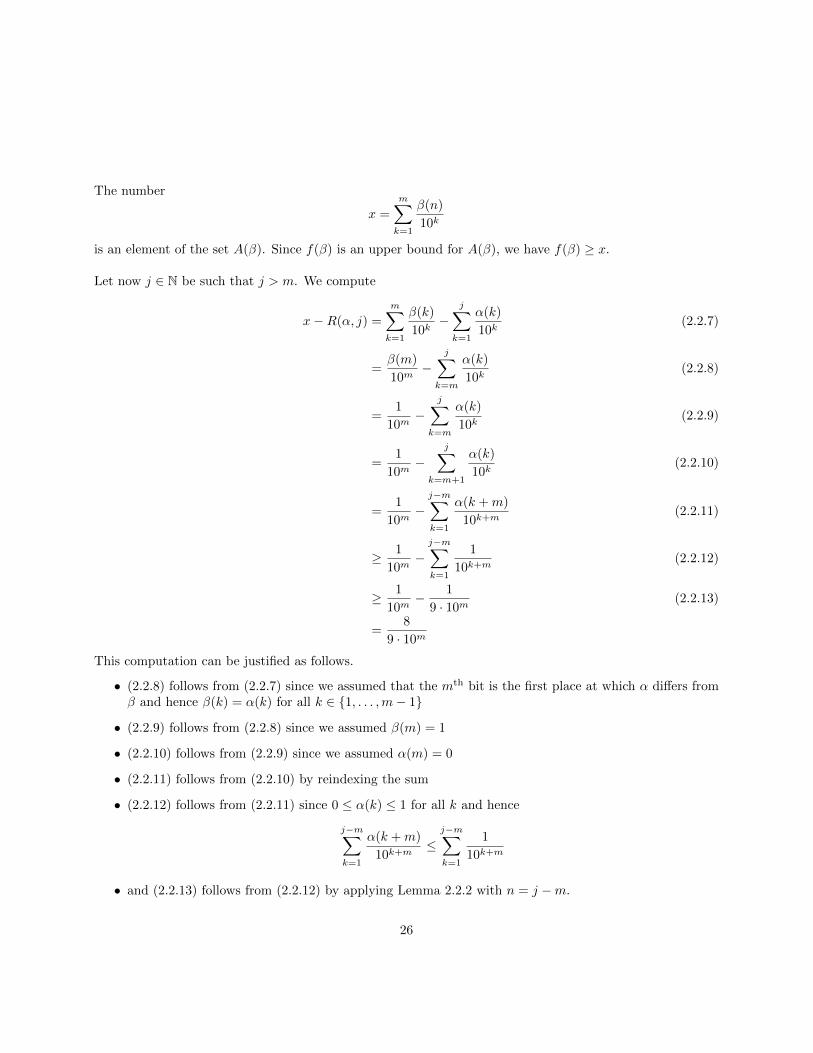
Let now j ∈ N be such that j > m. We compute

x−R(α, j) =

m∑k=1

β(k)

10k−

j∑k=1

α(k)

10k(2.2.7)

=β(m)

10m−

j∑k=m

α(k)

10k(2.2.8)

=1

10m−

j∑k=m

α(k)

10k(2.2.9)

=1

10m−

j∑k=m+1

α(k)

10k(2.2.10)

=1

10m−j−m∑k=1

α(k +m)

10k+m(2.2.11)

≥ 1

10m−j−m∑k=1

1

10k+m(2.2.12)

≥ 1

10m− 1

9 · 10m(2.2.13)

=8

9 · 10m

This computation can be justified as follows.

• (2.2.8) follows from (2.2.7) since we assumed that the mth bit is the first place at which α differs fromβ and hence β(k) = α(k) for all k ∈ {1, . . . ,m− 1}

• (2.2.9) follows from (2.2.8) since we assumed β(m) = 1

• (2.2.10) follows from (2.2.9) since we assumed α(m) = 0

• (2.2.11) follows from (2.2.10) by reindexing the sum

• (2.2.12) follows from (2.2.11) since 0 ≤ α(k) ≤ 1 for all k and hence

j−m∑k=1

α(k +m)

10k+m≤j−m∑k=1

1

10k+m

• and (2.2.13) follows from (2.2.12) by applying Lemma 2.2.2 with n = j −m.

26

The above computation shows that

x− 8

9 · 10m≥ R(α, j)

whenever j > m. Since R(α, `) ≤ R(α, j) when ` ≤ j it follows that

x− 8

9 · 10m≥ R(α, j)

for all j ∈ N. Therefore the number x− 89·10m is an upper bound for A(α).

Since f(β) ≥ x, it follows that the number f(β)− 89·10m is an upper bound for A(α). Since f(β)− 8

9·10m < f(β)we see that f(β) cannot be the least upper bound of A(α). By our definition of f , this implies that f(β) isdifferent from f(α). This completes the proof of Theorem 2.2.2

We emphasize that the function f was defined using least upper bounds. Since least upper bounds do notgenerally exist in the rational numbers the proof strategy of Theorem 2.2.2 fails when applied to the rationalnumbers. This is consistent with the countability of the rational numbers.

2.3 Absolute value and distance in the real line

In order to develop calculus we will need the notion of the absolute value of a real number. If x ∈ R, theabsolute value |x| is defined through cases by

|x| =

x if x > 0

0 if x = 0

−x if x < 0

Here are some elementary observations about the notion of absolute value.

• |x| ≥ 0 for all x ∈ R

• |xy| = |x||y|

• |x| = | − x|

• |x| = 0 implies x = 0

• If ε > 0, we have |x| ≤ ε if and only if −ε ≤ x ≤ ε

• More generally, we have |a− x| ≤ ε if and only if

a− ε ≤ x ≤ a+ ε (2.3.1)

The last property can be visualized as saying that the condition |a − x| ≤ ε defines a symmetric inter-val of radius ε centered at x. An interval delimited by ≤ is called an closed interval. The condition|a− x| < ε defines a open interval of radius ε centered at a. If a < b we can also define the closed interval[a, b] = {x ∈ R : a ≤ x ≤ b} and the open interval (a, b) = {x ∈ R : a < x < b}.

The following fact and its generalizations are the most important inequalites in all of mathematics.

27

Theorem 2.3.1 (triangle inequality). For all x, y ∈ R we have |x+ y| ≤ |x|+ |y|.

The triangle inequality gets its name because the two-dimensional version can be seen as asserting that thelength of any side of a triangle is no larger than the sum of the lengths of the two other sides.

Proof of Theorem 2.3.1. First we observe that we have −|x| ≤ x ≤ |x| and −|y| ≤ y ≤ |y|. (In each of thesecases one inequality is in fact an equality.) Adding these inequalities, we obtain

−(|x|+ |y|) ≤ x+ y ≤ |x|+ |y|.

We now consider two cases depending on the sign of x+ y.

Suppose first that x+ y ≥ 0. Then |x+ y| = x+ y ≤ |x|+ |y|.

Suppose now that x+y < 0. Then |x+y| = −(x+y). Since −(|x|+ |y|) ≤ x+y we have |x|+ |y| ≥ −(x+y).Thus we see that the theorem holds in both cases.

We define the distance between two real numbers x and y to be the nonnegative quantity |x− y|. Here arethe essential properties of the notion of distance.

• (distance is symmetric) For all x, y we have |x− y| = |y − x|

• (triangle inequality for distances) For all x, y, z we have

|x− z| ≤ |x− y|+ |y − z|

• (distance detects equality) We have |x− y| = 0 if and only if x = y.

These three properties define a structure called a metric. Metrics are ubiquitous in mathematics, as theyallow one to generalize intuitions about distance in the real line.

The next property is a powerful method for proving equalities between real numbers.

Theorem 2.3.2 (an ε of room again). If |x− y| ≤ ε for every ε > 0 then x = y.

Proof of Theorem 2.3.2. Theorem 2.1.2 asserted that if z, w ∈ R and w ≤ z + ε for every positive number εthen w ≤ z. If x and y are real numbers, we can apply the previous statement to z = 0 and w = |x− y| tosee that if |x − y| ≤ ε for every positive number ε then |x − y| ≤ 0. Since we always have |x − y| ≥ 0 thisimplies |x− y| = 0. Since distance detects equality we obtain x = y.

28

Chapter 3

Sequences and series

3.1 Sequences of real numbers

3.1.1 Basic information

We have now covered the basic theory of the real numbers themselves. The next level of structure we willconsider is the idea of a function from the natural numbers to the real numbers.

A function a : N → R is called a sequence. We will typically write an instead of a(n) and denote thewhole sequence as (an)∞n=1.

Here are some important examples of sequences.

• (constant sequence) Let an = 3 for all n ∈ N

• (sequence of natural numbers) Let an = n for all n ∈ N.

• (sequence of reciprocals of natural numbers) Let an = 1n for all n ∈ N.

The choice of the number 3 in the first example is incidental; we could also consider a constant sequencewith any other fixed value.

Since the natural numbers are infinite, it does not make sense to ask about the last element of a sequence.However, it is often possible to assert that the sequence approaches some final value as n goes to infinity. Ifthis is the case, we say that the sequence converges.

We now present the formal definition of convergence of a sequence. This is the first aspect of our discussionswhich can genuinely be considered calculus.

Definition 3.1.1. We say that a sequence (an)∞n=1 converges to a real number α if for every ε > 0 thereexists N ∈ N such that for all n ≥ N we have |an − α| ≤ ε.

We emphasize that the number N depends on ε.

29

The intuition behind this definition is that for any fixed error width ε, if we wait long enough then theall remaining terms of the sequence will lie within the interval of radius ε around the limiting value α.

If the sequence (an)∞n=1 converges to α, we denote this by writing limn→∞ an = α.

3.1.2 Examples

We now analyze the convergence behavior of our example sequences. The first example is trivial but illus-trative.

Proposition 3.1.1. Let an = 3 for all n. We have limn→∞ an = 3.

Proof of Proposition 3.1.1. Fix ε > 0. Choose N = 1. For all n ≥ 1 we have |an − 3| = 0 ≤ ε.

Notice that this example would be mostly the same if we defined a1 = 7, a2 = 9 and an = 3 for all n ≥ 3. Inthat case we would instead choose N = 3.

The next case is the essential example of a nontrivial convergent sequence.

Proposition 3.1.2. Let an = 1n for all n. We have limn→∞ an = 0.

Proof of Proposition 3.1.2. Fix ε > 0. We can consider the positive real number 1ε .

We claim that there exists a natural number N such that N ≥ 1ε . Suppose toward a contradiction that

the claim failed. Then 1ε would be an upper bound for the set of natural numbers.

By Axiom 14, there must exist a least upper bound x for N. Since x is the least upper bound, x − 1cannot be an upper bound. Therefore there must be a natural number m such that x− 1 < m. This impliesthatm+1 > x. Sincem+1 is a natural number, this contradicts the hypothesis that x is an upper bound for N.

Using the claim, we can choose a natural number N such that N ≥ 1ε . We need to show that for all

n ≥ N we have |an − 0| ≤ ε.

Suppose n ≥ N . Then

|an − 0| = |an| =∣∣∣∣ 1n∣∣∣∣ =

1

n≤ 1

N≤ ε.

This verifies Definition 3.1.1 and completes the proof of Proposition 3.1.2

The next case is the essential example of a sequence which does not converge.

Proposition 3.1.3. Let an = n for all n. This sequence does not converge to any limit.

Proof of Proposition 3.1.3. Suppose toward a contradiction that there exists some real number α such thatlimn→∞ n = α.

Setting ε = 1 in the definition of convergence, this implies that there exists N such that |n − α| ≤ 1for all n ≥ N . In particular, we must have |N − α| ≤ 1 so that the left side of (2.3.1) implies N ≥ α− 1.

30

Let n = N + 3. Then we have n ≥ α − 1 + 3 = α + 2. This implies in particular that n − α is non-negative and so |n− α| = n− α ≥ 2.

This contradicts our assumption that |n − α| ≤ 1 for all n ≥ N . Since α was an arbitrary real number,the sequence (an)∞n=1 does not converge to any limit.

3.1.3 Uniqueness of limits of sequences

An important fact is that if a sequence has a limit, then that limit must be unique.

Theorem 3.1.1. Suppose (an)∞n=1 is a sequence of real numbers such that limn→∞ an = α and limn→∞ an =β. Then α = β.

Proof of Theorem 3.1.1. Let (an)∞n=1 and α, β be as in the statement of Theorem 3.1.1.

Fix ε > 0. Since limn→∞ an = α, we can find N such that for all n ≥ N we have |an − α| ≤ ε2 . Since

limn→∞ an = β, we can find M such that for all n ≥M we have |an − β| ≤ ε2 .

Choose n ≥ max(N,M). Using the triangle inequality we have

|α− β| ≤ |α− an|+ |an − β| = |an − α|+ |an − β| ≤ε

2+ε

2= ε.

Since ε > 0 was arbitrary, Theorem 2.3.2 implies α = β as required.

The proof of Theorem 3.1.1 demonstrates two important analytic techniques. First of all, we see the fun-damental utility of Theorem 2.3.2. Secondly, we used the idea of choosing an initial positive value of ε andthen applying the definition of convergence to a smaller positive quantity, in this case ε

2 .

3.1.4 Arithmetic of sequences

We now state the basic rules that describe how limits of sequences interact with arithmetic.

Theorem 3.1.2. Suppose (an)∞n=1 and (bn)∞n=1 are sequences such that limn→∞ an = α and limn→∞ bn = β.

• We have limn→∞(an + bn) = α+ β.

• We have limn→∞ anbn = αβ.

We will prove the second of these rules. The first can be proved in a similar way.

Proof of second clause in Theorem 3.1.2. Let (an)∞n=1, (bn)∞n=1 and α, β be as in the statement of Theorem3.1.2.

By applying the definition of convergence to ε = 1, we see that there exists N such that |an − α| ≤ 1for all n ≥ N . This implies ||an| − |α|| ≤ 1 so that from the right side of (2.3.1) we obtain |an| ≤ |α|+ 1 forall n ≥ N . Again applying the definition of convergence we can find N ′ such that

|an − α| ≤ε

2(|β|+ 1)

31

for all n ≥ N ′. Similarly, we can find M such that

|bn − β| ≤ε

2(|α|+ 1)

for all n ≥M .

Let K = max(N,N ′,M) and consider n ≥ K. We have

|anbn − αβ| ≤ |anbn − anβ|+ |anβ − αβ| (3.1.1)

= |an| · |bn − β|+ |an − α| · |β| (3.1.2)

≤ (|α|+ 1) · |bn − β|+ |an − α| · |β| (3.1.3)

≤ (|α|+ 1) · ε

2(|α|+ 1)+ |an − α| · |β| (3.1.4)

≤ (|α|+ 1) · ε

2(|α|+ 1)+

ε

2(|β|+ 1)· |β| (3.1.5)

≤ ε

2+ε

2= ε

This computation can be justified as follows.

• The inequality in (3.1.1) follows from the triangle inequality (Theorem 2.3.1)

• (3.1.3) follows from (3.1.2) by our choice of N

• (3.1.4) follows from (3.1.3) by our choice of M

• and (3.1.5) follows from (3.1.4) by our choice of N ′

Thus we have shown limn→∞ anbn = αβ as desired.

In the above proof we used a more sophisticated version of the ‘ ε2 ’ idea by applying the definition of conver-gence to quantities such as ε

2(|β|+1) .

3.1.5 Squeeze theorem

We now state a theorem which is crucial for computing many limits.

Theorem 3.1.3 (Squeeze theorem). Let (an)∞n=1, (bn)∞n=1 and (cn)∞n=1 be sequences. Suppose there existsM ∈ N such that an ≤ bn ≤ cn for all n ≥ M . Then if limn→∞ an = α = limn→∞ cn we also havelimn→∞ bn = α.

Proof of Theorem 3.1.3. Let ε > 0. Since limn→∞ an = α, we can find N ∈ N such that |an − α| ≤ ε for alln ≥ N . In particular, we have an ≥ α− ε. It follows that if n ≥ max(M,N) then we have bn ≥ an ≥ α− ε.

Since limn→∞ cn = α we can find N ′ ∈ N such that |cn − α| ≤ ε for all n ≥ N ′. In particular, wehave cn ≤ α+ ε. It follows that if n ≥ max(M,N ′) then an ≤ cn ≤ α+ ε.

Therefore if n ≥ max(M,N,N ′) then we will have α−ε ≤ an ≤ α+ε. By (2.3.1) this implies |an−α| ≤ ε.

32

We now consider an example of how we can apply the squeeze theorem.

Proposition 3.1.4. Let

bn =(−1)n + (−1)n

2

n

for all n. Then limn→∞ bn = 0.

Proof of Proposition 3.1.4. If we tried to work directly with the sequence (bn)∞n=1, this result would bedifficult to prove due the oscillations of the numerator. Instead, we define sequences an = − 2

n and cn = 2n .

Observe that for all n we have−2 ≤ (−1)n + (−1)n

2

≤ 2

so that an ≤ bn ≤ cn.

From Proposition 3.1.2 we have limn→∞1n = 0. By applying the second clause of Theorem 3.1.2 to the

constant sequences with values −2 and 2 respectively, we see that

limn→∞

an = −2 · 0 = 0 = 2 · 0 = limn→∞

cn

Thus we can apply Theorem 3.1.3 to conclude that limn→∞ bn = 0.

3.1.6 Monotone sequences

A special class of sequences that are particularly tractable are monotone sequences. We say that a sequence(an)∞n=1 is increasing if an ≤ an+1 for all n ∈ N. Similarly, we say that (an)∞n=1 is decreasing if an ≥ an+1

for all n ∈ N. We say a sequence is monotone if it is increasing or decreasing.

Theorem 3.1.4 (Convergence of monotone sequences). Suppose (an)∞n=1 is an increasing sequence whichhas an upper bound for its terms. Then (an)∞n=1 converges to its least upper bound. Similarly, if (an)∞n=1 isa decreasing sequence which has a lower bound, then it converges to its greatest lower bound.

Proof of Theorem 3.1.4. We will prove the increasing case of this theorem. The decreasing case follows byapplying the increasing case to the sequence (−an)∞n=1. Suppose (an)∞n=1 is an increasing sequence with anupper bound. Let α be the least upper bound for the terms of (an)∞n=1.

Let ε > 0. We must find N ∈ N such that |an − α| ≤ ε for all n ≥ N . Notice that since an ≤ α forall n, it suffices to show that an ≥ α− ε for all n ≥ N .

Since α is the least upper bound for the terms of (an)∞n=1, we know that α − ε cannot be an upper bound.Therefore there exists some aN such that aN ≥ α−ε. Since (an)∞n=1 is increasing, this implies that an ≥ α−εfor all n ≥ N as desired.

3.1.7 Subsequences and the Bolzano-Weierstrass theorem

A subsequence of the natural numbers is an infinite list

n1 < n2 < n3 < · · · < nk < nk+1 < · · ·

33

where each nk ∈ N. For example, we could choose nk = 3k or nk = 2k.

If (an)∞n=1 is a sequence of real numbers, a subsequence of (an)∞n=1 is a sequence which has the form (ank)∞k=1

for some subsequence (nk)∞k=1 of the natural numbers. Intuitively, a subsequence of (an)∞n=1 is obtained byforgetting some of the terms of (an)∞n=1.

For example, consider the sequence an = 1/n. The sequence

1,1

3,

1

9,

1

27, · · · , 1

3k, · · ·

is a subsequence of (an)∞n=1. On the other hand, the sequence

1,1

3,

1

2,

1

9,

1

27,

1

81, · · ·

is not a subsequence of (an)∞n=1. Even though each term of this latter sequence is also a term of (an)∞n=1, thefact that 1/3 and 1/2 are in the wrong order prevents this from being a subsequence.

Lemma 3.1.1 (existence of monotone subsequences). Every sequence of real numbers has a monotone sub-sequence.

Proof of Lemma 3.1.1. Let (an)∞n=1 be a sequence of real numbers. We need to find a monotone subsequence.The key idea is the following definition. We say that a term an is a peak of the sequence if an ≥ am for allm ≥ n. In other words, an is at least as big as any term which follows it.

For example, every term of a decreasing sequence is a peak. On the other hand, an increasing sequencehas a peak only if it is eventually constant. We will consider two cases, depending on whether the set ofpeaks is finite or infinite.

Case 1 (finitely many peaks) In this case we assume that the set of peaks of (an)∞n=1 is finite. We willrecursively build an increasing subsequence. Since the set of peaks is finite, we can find N such that if n ≥ Nthen an is not a peak. We choose the first index for our subsequence as n1 = N .

Since n1 > N , we know that an1is not a peak. Therefore there exists n2 > n1 such that an2

> an1.

Since n2 is also greater than N , we know that an2is not a peak. Therefore there exists n3 > n2 such that

an3> an2

. Continuing in this way, we find an increasing subsequence.

Case 2 (infinitely many peaks) In this case we assume that the set of peaks of (an)∞n=1 is infinite. Wewill build a decreasing subsequence.

Let n1 < n2 < n3 < · · · be the sequence of indexes of peaks. We claim that the sequence an1, an2

, an3, . . .

is decreasing. This follows from the definition of a peak: since each ankis a peak, we have ank

≥ am for allm ≥ nk. In particular, this implies ank+1

≤ ank.

In either case, we have found a monotone subsequence. This completes the proof of Lemma 3.1.1

We will say that a sequence is bounded if there is an upper bound for the absolute values of its terms.Equivalently, there is both an upper and lower bound for the terms. The following theorem will be crucialto many later arguments.

34

Theorem 3.1.5 (Bolzano-Weierstrass theorem). Every bounded sequence of real numbers has a convergentsubsequence.

Proof of Theorem 3.1.5. Let (an)∞n=1 be a sequence of real numbers. By Lemma 3.1.1 there exists a monotonesubsequence (ank

)∞k=1. Since (an)∞n=1 is bounded the sequence (ank)∞k=1 is also bounded. Therefore Theorem

3.1.5 follows from Theorem 3.1.4

3.1.8 Cauchy sequences

In order to verify the definition of convergence directly, one needs to know in advance what the limit shouldbe. It would useful to know a criterion for convergence which does not have this requirement. We nowpresent such a criterion

Definition 3.1.2. We say that a sequence (an)∞n=1 is a Cauchy sequence if for every ε > 0 there existsN ∈ N such that for all n,m ≥ N we have |an − am| ≤ ε.The importance of Cauchy sequences is captured by the following theorem.

Theorem 3.1.6. A sequence of real numbers converges if and only if it is a Cauchy sequence

Proof of Theorem 3.1.6. The theorem asserts an equivalence, so we have two implications to prove.

Convergence implies Cauchy Suppose that (an)∞n=1 is a convergent sequence with limn→∞ an = α. Letε > 0. By the definition of convergence, we can find N such that if n ≥ N then |an − α| ≤ ε

2 .

In particular, if n,m ≥ N then we have |an − α| ≤ ε2 and |am − α| ≤ ε

2 so that

|an − am| ≤ |an − α|+ |am − α| ≤ε

2+ε

2= ε.

Thus we have verified the definition of a Cauchy sequence.

Cauchy implies convergence We claim first that every Cauchy sequence is bounded. Let (an)∞n=1 bea Cauchy sequence. By the definition of a Cauchy sequence, we can find N ∈ N such that if n ≥ N then|aN − an| ≤ 1. In particular, if n ≥ N then we have |an| ≤ |aN |+ 1. Define C = max(|a1|, |a2|, . . . , |aN |) + 1.Then |an| ≤ C for all n so (an)∞n=1 is bounded.

We now claim that if a Cauchy sequence has a convergent subsequence, then the original sequence con-verges. Let (an)∞n=1 be a Cauchy sequence and let (ank

)∞k=1 be a subsequence with limk→∞ ank= α.

Let ε > 0. By the definition of a Cauchy sequence, we can find N ∈ N such that if n,m ≥ N then|an − am| ≤ ε

2 . By the definition of convergence, we can find K ∈ N such that if k ≥ K then |ank− α| ≤ ε

2 .

Since (nk)∞k=1 is a subsequence of the natural numbers, we can find k ≥ K such that nk ≥ N . Thenfor any m ≥ N we have

|am − α| ≤ |am − ank|+ |ank

− α| ≤ ε

2+ε

2= ε.

This completes the proof of the second claim.

Now, let (an)∞n=1 be a Cauchy sequence. Since (an)∞n=1 is bounded, Theorem 3.1.5 implies that (an)∞n=1

has a convergent subsequence. Therefore the second claim implies that (an)∞n=1 converges.

35

3.2 Infinite sums

3.2.1 Basic information

The associativity axiom for addition allows us to unambiguously define the sum of any finite list of realnumbers. However, it is important in many contexts to consider infinite sums. We can give a precisedefinition of an infinite sum using our definition of convergence for sequences.

Definition 3.2.1. Let (an)∞n=1 be a sequence of real numbers. We say that the infinite sum

∞∑n=1

an

converges if the sequence of finite partial sums

bk =

k∑n=1

an

converges as k →∞.

Suppose that this is the case, and write α for limk→∞ bk. We think of α as the exact value of the infi-nite sum, and we write

∞∑n=1

an = α

Often an infinite sum is called a series.

3.2.2 Zero test

Proposition 3.2.1. A necessary condition for a series∑∞n=1 an to converge is that limn→∞ an = 0.

Proof of Proposition 3.2.1. Suppose toward a contradiction that Proposition 3.2.1 fails. Let (an)∞n=1 be asequence of real numbers which does not converge to zero. Negating the definition of convergence, we seethat there exists some ε > 0 such that for an infinite set J ⊆ N and all k ∈ J we have |ak| ≥ ε.

This implies that if k ∈ J we have ∣∣∣∣∣k−1∑n=1

an −k∑

n=1

an

∣∣∣∣∣ = |ak| ≥ ε.

Therefore the partial sums∑kn=1 an cannot form a Cauchy sequence and so Theorem 3.1.6 implies the series

does not converge.

3.2.3 Examples

Geometric series

Proposition 3.2.2. Let 0 < b < 1. Then we have

∞∑n=1

bn =b

1− b

36

Proof of Proposition 3.2.2. In order to prove Proposition 3.2.2, we need to examine the finite partial sums.By applying Lemma 2.2.1 we see that

k∑n=1

bk =1− bk+1

1− b− 1 =

b− bk+1

1− b

Since b < 1 we have limk→∞ bk+1 = 0, so

limk→∞

b− bk+1

1− b=

b

1− b

Thus we have shown∞∑n=1

bn =b

1− b

Harmonic series

The following example shows that the condition that limn→∞ an = 0 is not sufficient for the series∑∞n=1 an

to converge.

Proposition 3.2.3. The series∑∞n=1

1n diverges.

Proof of Proposition 3.2.3. We group the terms of the series into blocks whose lengths are powers of two:

∞∑n=1

1

n= 1 +

(1

2+

1

3

)+

(1

4+

1

5+

1

6+

1

7

)+

(1

8+ · · ·+ 1

15

)+ · · ·

Each term in the kth block is at least 12k

. Thus we see that

∞∑n=1

1

n≥ 1 +

(1

4+

1

4

)+

(1

8+

1

8+

1

8+

1

8

)+

(1

16+ · · ·+ 1

16

)+ · · ·

Since there are 2k−1 terms in the kth block, we see that the sum of each block is at least 12 and therefore

∞∑n=1

1

n≥ 1 + 2 · 1

4+ 4 · 1

8+ 8 · 1

16+ · · ·

= 1 +1

2+

1

2+

1

2+ · · · =∞.

Basel series

In the next example we will need to exploit the Cauchy criterion in order to prove convergence.

Proposition 3.2.4. The series∑∞n=1

1n2 converges.

37

For historical reasons, this is called the Basel series.

Proof of Proposition 3.2.4. Let ε > 0 and choose N ∈ N such that 1N ≤ ε. We claim that if k,m ≥ N then∣∣∣∣∣

k∑n=1

1

n2−

m∑n=1

1

n2

∣∣∣∣∣ ≤ ε.This will show that the partial sums of the series form a Cauchy sequence, and therefore we can concludethat the series converges.

Let k,m ≥ N and assume without loss of generality that m > k. We compute:∣∣∣∣∣k∑

n=1

1

n2−

m∑n=1

1

n2

∣∣∣∣∣ =

m∑n=k+1

1

n2

≤m∑

n=k+1

1

n(n− 1)

=

m∑n=k+1

(1

n− 1− 1

n

)

=

m∑n=k+1

1

n− 1−

m∑n=k+1

1

n

=

m−1∑n=k

1

n−

m∑n=k+1

1

n(3.2.1)

=1

k− 1

m(3.2.2)

≤ 1

N≤ ε

Here in passing from (3.2.1) to (3.2.2) we cancelled a telescoping sum.

We have shown that∞∑n=1

1

n2

converges, but we haven’t computed the value of the sum. Determining this value was considered one of themost significant challenges in mathematics during the eighteenth century. The problem was solved by a mannamed Leonhard Euler, who is universally regarded as one of the greatest mathematicians of all time.

38

The solution is∞∑n=1

1

n2=π2

6

3.2.4 Convergence criteria

We now develop some general techniques for analyzing the convergence behavior of infinite series.

Absolute convergence

Theorem 3.2.1. Suppose∑∞n=1 |an| converges. Then

∑∞n=1 an converges.

Proof of Theorem 3.2.1. Assume that∑∞n=1 |an| converges. Then the partial sums

∑kn=1 |an| form a Cauchy

sequence.

Let ε > 0. We can find N such that if k,m ≥ N we have∣∣∣∣∣k∑

n=1

|an| −m∑n=1

|an|

∣∣∣∣∣ ≤ ε.Assume without loss of generality that m > k. Using the triangle inequality we have∣∣∣∣∣

m∑n=1

an −k∑

n=1

an

∣∣∣∣∣ =

∣∣∣∣∣m∑

n=k+1

an

∣∣∣∣∣ ≤m∑

n=k+1

|an|

=

m∑n=1

|am| −k∑

n=1

|am|

=

∣∣∣∣∣m∑n=1

|am| −k∑

n=1

|am|

∣∣∣∣∣ ≤ εTherefore the partial sums of

∑∞n=1 an form a Cauchy sequence and so the series converges.

If∑∞n=1 |an| converges we say that

∑∞n=1 an converges absolutely.

Comparison test

Theorem 3.2.2. Suppose that there exists N ∈ N such that 0 ≤ an ≤ bn for all n ≥ N . If∑∞n=1 bn converges

then∑∞n=1 an converges. If

∑∞n=1 an diverges then

∑∞n=1 bn diverges.

We leave the proof of the validity of this test as an optional exercise.

The comparison test can be used in a similar way to the squeeze theorem to convert more complicatedseries to simpler ones. We now give an example of this.

Proposition 3.2.5. The series∞∑n=1

1

n2 + 2n− 5

converges.

39

Proof of Proposition 3.2.5. If n ≥ 3 then 2n− 5 > 0 so that

1

n2 + 2n− 5≤ 1

n2.

Since∞∑n=1

1

n2

converges, we see that∞∑n=1

1

n2 + 2n− 5

converges.

Ratio test

Theorem 3.2.3. Let (an)∞n=1 be a sequence of nonzero real numbers. Suppose that there exists N ∈ N andr < 1 such that |an+1

an| ≤ r for all n ≥ N . Then

∑∞n=1 an converges. On the other hand, suppose that there

exists N ∈ N such that |an+1

an| ≥ 1 for all n ≥ N . Then

∑∞n=1 an does not converge.

Proof of Theorem 3.2.3. Suppose first that there exists N ∈ N and r < 1 such that |an+1

an| ≤ r for all n ≥ N .

By induction we can see that this implies |an| ≤ rn−N |aN | for all n ≥ N . Therefore we have

∞∑n=1

|an| =N∑n=1

|an|+∞∑

n=N+1

|an|

≤N∑n=1

|an|+∞∑

n=N+1

rn−N |aN |

=

N∑n=1

|an|+ |aN | ·∞∑m=1

rm

Since∑Nn=1 |an| is a finite number, it does not affect the convergence behavior of the series. The series∑∞

n=1 rm is a geometric series and is hence convergent by Proposition 3.2.2. Therefore

∑∞n=1 an converges.

Suppose now that there exists N ∈ N such that |an+1

an| ≥ 1 for all n ≥ N . Equivalently, this means

that |an+1| ≥ |an|. Therefore |an| ≥ |aN | > 0 for all n ≥ N . Since the individual terms of the sequence donot approach zero, we see that

∑∞n=1 an cannot converge.

We now give an example of how to apply Theorem 3.2.3.

Proposition 3.2.6. Let an = n4n+3 . Then the series

∑∞n=1 an converges.

Proof of Proposition 3.2.6. We compute∣∣∣∣an+1

an

∣∣∣∣ =

∣∣∣∣n+ 1

4n+4· 4n+3

n

∣∣∣∣ =n+ 1

n· 1

4=

(1 +

1

n

)· 1

4.

40

Since 1 + 1n ≤ 2, we see that ∣∣∣∣an+1

an

∣∣∣∣ ≤ 1

2

for all n. Therefore Theorem 3.2.3 implies that

∞∑n=1

n

4n+3

converges.

Root test

Theorem 3.2.4. Let (an)∞n=1 be a sequence of real numbers. Suppose that there exists N ∈ N and r < 1such that |an| ≤ rn for all n ≥ N . Then

∑∞n=1 an converges.

Theorem 3.2.4 can be established in a similar way to Theorem 3.2.3, using comparison with a geometric series.

We now consider an example of how to apply Theorem 3.2.4.

Proposition 3.2.7. Let an = 311nn−n. Then the∑∞n=1 an converges.

Proof of Proposition 3.2.7. Suppose n ≥ 311 + 1. Then we have

an =

(311

n

)n≤(

311

311 + 1

)n.

Letting r = 311

311+1 < 1 we can apply the root test to conclude that

∞∑n=1

311n

nn

converges.

41

Chapter 4

Limits and continuity

4.1 Functions of a real variable

We will now begin to discuss the main subject of this text: functions from a subset of the real numbers tothe real numbers.

If A ⊆ R and f is a function from A to R, we refer to A as the domain of the function f . We think ofA as being the set of real numbers for which the function f is defined. In many cases, A will be the wholeset of real numbers. In this case we say that the function is defined everywhere.

4.1.1 Examples

We now give some basic examples of classes of functions.

Polynomials

Polynomials are functions which have the form

f(x) = c0 + c1x+ c2x2 + · · ·+ cn−1x

n−1 + cnxn

where c0, . . . , cn are fixed real numbers. A polynomial is defined everywhere. Below are some explicitexamples of polynomials.

• f(x) = x

• f(x) = 7x5 − 3x− 19

• f(x) =

153∑k=0

(−1)k

k13 + 1x4k

The highest power of the variable which appears in a polynomial is called the degree of the polynomial. Thedegrees of the examples above are 1, 5 and 612 = 153 · 4 respectively.

Constant functions are considered polynomials of degree zero.

42

Rational functions

Rational functions have the form f(x) = p(x)q(x) where p and q are polynomials. Such a rational function is

defined for all x with q(x) 6= 0.

Taking q to be the constant function with value 1, we see that polynomials are a special case of rationalfunctions. Below are some explicit examples of rational functions which are not polynomials.

• f(x) =1

x

• f(x) =7x3 − 11x+ 4

(x− 3)(x+ 8)

• f(x) =−19x4

x2 + 1

The first example is defined for all nonzero x. The second example is defined for all x except 3 and −8. Thethird example is defined everywhere, since the quantity x2 + 1 is always positive.

Absolute value

We can consider the function f(x) = |x|. More generally, if a is a fixed real number, we can consider thefunction f(x) = |x− a|. We think of this function as expressing the distance from x to the point a.

Indicator functions

If B ⊆ R, we can define a function f : R→ R by setting

f(x) =

{1 if x ∈ B0 if x /∈ B

This function is called the indicator of B. As the name suggests, indicator functions give a way of identifyingsubsets of the real numbers.

4.1.2 Operations on functions

There are some basic operations we can perform to make new functions out of old ones.

Arithmetic operations

If f : A → R and g : A → R, we can define the sum f + g by (f + g)(x) = f(x) + g(x). Similarly, we can

define the product fg by (fg)(x) = f(x)g(x). We can also define the quotient fg by

(fg

)(x) = f(x)

g(x) for inputs

x with g(x) 6= 0.

All rational functions can be built from constant functions and the function f(x) = x using these oper-ations.

43

Compositions

Suppose f : A → R and g : B → R are functions such that f(A) ⊆ B. Then we can define the compositiong ◦ f : A→ R by (g ◦ f)(x) = g(f(x)).

For example, let f(x) = x3 − 3 and g(x) = x2 + x+ 7. Then we have

(g ◦ f)(x) = g(f(x))

= g(x3 − 3)

= (x3 − 3)2 + (x3 − 3) + 7

= x6 − 5x3 + 13

Piecewise definitions

Suppose f : A → R and g : B → R are functions such that f(x) = g(x) whenever x ∈ A ∩ B. Then we candefine a piecewise function h : A ∪B → R by letting

h(x) =

{f(x) if x ∈ Ag(x) if x ∈ B

In particular, if A and B are disjoint, then we can make a piecewise definition of a function on A∪B for anypair of functions f : A→ R and g : B → R.

More generally, if A1, . . . , An are pairwise disjoint sets and fk : Ak → R are functions, then we can make apiecewise definition of a function g : A1 ∪ · · · ∪An → R by letting g(x) = fk(x) for x ∈ Ak.

4.2 Limits

4.2.1 Basic information

Definition 4.2.1. Let A ⊆ R. We say that a point a ∈ R is a cluster point of A if for every δ > 0 thereexists x ∈ A with |x− a| ≤ δ.

Intuitively, a point a is a cluster point of a set A if there exist points in A which are arbitrarily close to a.

Definition 4.2.2. Let f : A→ R be a function and let a ∈ R be a cluster point of A. We say that the limitof f as x approaches a is equal to α if the the following condition is satisfied. For every ε > 0 there existsδ > 0 such that if x ∈ A and |x− a| ≤ δ then |f(x)− α| ≤ ε. If this is the case, we write limx→a f(x) = α.

We emphasize that the number δ depends on ε.

The hypothesis that a is a cluster point of A is necessary in order to rule out the possibility that theconditions |x− a| ≤ δ and x ∈ A are incompatible for some positive value of δ. When we discuss limits, wewill always implicitly assume that the limit point is a cluster point of the domain.

44

4.2.2 Uniqueness of limits

Theorem 4.2.1. Let f : A → R be a function and suppose limx→a f(x) = α and limx→a f(x) = β. Thenα = β.

Proof of Theorem 4.2.1. Let ε > 0. Applying the definition of the limit to α, we see that there exists δ > 0such that if x ∈ A and |x− a| ≤ δ then |f(x)− α| ≤ ε

2 .

Applying the definition of the limit to β, we see that there exists δ′ > 0 such that if x ∈ A and |x− a| ≤ δ′

then |f(x)− β| ≤ ε2 .

Let δ′′ = min(δ, δ′) > 0. Since a is a cluster point of A, we can choose x ∈ A such that |x − a| ≤ δ′′.We have

|α− β| ≤ |α− f(x)|+ |f(x)− β| ≤ ε

2+ε

2= ε.

4.2.3 Examples

We now give some examples of limits of functions.

Identity function

The first example is trivial but illustrative.

Proposition 4.2.1. Let f(x) = x. Then for any point a ∈ R we have limx→a f(x) = a.

Proof of Proposition 4.2.1. Let ε > 0 and choose δ = ε. Then |x−a| ≤ δ implies |f(x)−a| = |x−a| ≤ ε.

Cube function

Proposition 4.2.2. Let f(x) = x3. Then limx→2 f(x) = 8.

Proof of Proposition 4.2.2. Let ε > 0. We need to find δ > 0 such that if |x− 2| ≤ δ then |x3 − 8| ≤ ε.

Set δ = min(ε19 , 1

)and suppose |x − 2| ≤ δ. In particular, this implies |x − 2| ≤ 1 so that |x| ≤ 3.

We have

|x3 − 8| = |(x− 2)(x2 + 2x+ 4)|= |x− 2| · |x2 + 2x+ 4|≤ |x− 2| · (|x|2 + 2|x|+ 4)

≤ |x− 2| · (32 + 2 · 3 + 4)

= 19 · |x− 2| ≤ 19δ ≤ ε

45

A rational function

Proposition 4.2.3. Let

f(x) =x3 − 3x2 − 4x+ 12

x− 3

Then limx→3 f(x) = 5.

The domain of the function f in Proposition 4.2.3 is A = {x ∈ R : x 6= 3}. We want to evaluate limx→3 f(x).Since the limit point 3 is a cluster point of A the limit is well-defined.

Proof of Proposition 4.2.3. Let ε > 0. We need to find δ > 0 such that if |x− 3| ≤ δ then∣∣∣∣x3 − 3x2 − 4x+ 12

x− 3− 5

∣∣∣∣ ≤ ε.We set δ = min

(ε7 , 1). This implies in particular that if |x− 3| ≤ δ then |x− 3| ≤ 1 and hence |x| ≤ 4.

Suppose x ∈ A and |x− 3| ≤ δ. We compute∣∣∣∣x3 − 3x2 − 4x+ 12

x− 3− 5

∣∣∣∣ =

∣∣∣∣ (x− 3)(x2 − 4)

x− 3− 5

∣∣∣∣ (4.2.1)

= |x2 − 9| = |x− 3| · |x+ 3| (4.2.2)

≤ |x− 3| · (|x|+ 3)

≤ 7 · |x− 3| ≤ 7δ ≤ ε.

Here our cancellation of the x− 3 factors in passing from (4.2.1) to (4.2.2) is justified since the assumptionthat x ∈ A implies x− 3 6= 0.

Sign function

We now consider an example where a limit does not exist.

Proposition 4.2.4. Define

f(x) =

1 if x > 0

0 if x = 0

−1 if x < 0

Then limx→0 f(x) does not exist.

The function f in Proposition 4.2.4 is sometimes called the sign function.

Proof of Proposition 4.2.4. Suppose toward a contradiction that there were α ∈ R such that limx→0 f(x) = α.Applying the definition of the limit with ε = 1

2 , we see that there exists δ > 0 such that if |x| ≤ δ then|f(x)− α| ≤ 1

2 .In particular, this implies that

|f(δ)− f(−δ)| ≤ |f(δ)− α|+ |α− f(−δ)| ≤ 1

2+

1

2= 1. (4.2.3)

On the other hand, we have |f(δ)− f(−δ)| = |1− (−1)| = 2, which contradicts (4.2.3).

46

Note that the fact f(x) = 0 played no role in the proof of Proposition 4.2.4. We could define f(0) to be anyreal number and the limit would still fail to exist. We could also leave f undefined at 0. This illustrates animportant idea: limits depend on the behavior of the function nearby the limit point, and not on the valueat the limit point itself.

4.2.4 Manipulation of limits

The rules for arithmetically manipulating limits of functions are identical to the rules for manipulating limitsof sequences. The proofs are similar.

Theorem 4.2.2. Suppose f : A→ R and g : A→ R are functions, suppose a is a cluster point of A, supposelimx→a f(x) = α and suppose limx→b g(x) = β.

• We have limx→a(f + g)(x) = α+ β.

• We have limx→a(fg)(x) = αβ.

• If β 6= 0 we have limx→a

(fg

)(x) = α

β .

Proof of Theorem 4.2.2. We prove the second of these rules; the proof of the first and third are similar. Letε > 0. Since limx→a f(x) = α we see there exists δ > 0 such that if |x − a| ≤ δ then |f(x) − α| ≤ 1 and so|f(x)| ≤ |α|+ 1. Again using the hypothesis that limx→a f(x) = α we see that there exists δ′ > 0 such thatif |x− a| ≤ δ′ then

|f(x)− α| ≤ ε

2(|β|+ 1)

Finally, using the hypothesis that limx→a g(x) = β we see that there exists γ > 0 such that |x− a| ≤ γ| then

|g(x)− β| ≤ ε

2(|α|+ 1)

Suppose |x− a| ≤ min(δ, δ′, γ). We compute

|f(x)g(x)− αβ| ≤ |f(x)g(x)− f(x)β|+ |f(x)β − αβ| (4.2.4)

= |f(x)| · |g(x)− β|+ |f(x)− α|β (4.2.5)

≤ (|α|+ 1)|g(x)− β|+ |f(x)− α|β (4.2.6)

≤ (|α|+ 1)ε

2(|α|+ 1)+ |f(x)− α|β (4.2.7)

≤ (|α|+ 1)ε

2(|α|+ 1)+

εβ

2(|β|+ 1)(4.2.8)

≤ ε

2+ε

2= ε

This computation can be justified as follows.

• The inequality in (4.2.4) follows from the triangle inequality (Theorem 2.3.1)

• (4.2.6) follows from (4.2.5) by our choice of δ

• (4.2.7) follows from (4.2.6) by our choice of δ′

• and (4.2.8) follows from (4.2.7) by our choice of γ.

47

4.2.5 Squeeze theorem

We also have an analog of the squeeze theorem.

Theorem 4.2.3. Suppose f : A → R, g : A → R and h : A → R are functions. Further suppose that thereexists γ > 0 such that if |x− a| ≤ γ then f(x) ≤ g(x) ≤ h(x). If limx→a f(x) = α and limx→a h(x) = α thenwe also have limx→a g(x) = α.

Proof of Theorem 4.2.3. Let ε > 0. Since limx→a f(x) = α we see there exists δ > 0 such that if |x− a| ≤ δthen |f(x) − α| ≤ ε. In particular, this implies f(x) ≥ α − ε. Therefore if |x − a| ≤ min(γ, δ) we will haveg(x) ≥ f(x) ≥ α− ε.

Since limx→a h(x) = β we see there exists δ′ > 0 such that if |x − a| ≤ δ′ then |h(x) − α| ≤ ε. In par-ticular, this implies h(x) ≤ α+ ε. Therefore if |x− a| ≤ min(γ, δ′) we will have f(x) ≤ h(x) ≤ α+ ε.

It follows that if |x − a| ≤ min(γ, δ, δ′) we will have α − ε ≤ f(x) ≤ α + ε. By (2.3.1) we see this im-plies |f(x)− α| ≤ ε.

4.2.6 Extended limits

We now discuss some important extensions of the limit concept.

Limits to infinity

Definition 4.2.3. Let f : A → R be a function. We say that limx→a f(x) = ∞ if for every M < ∞ thereexists δ > 0 such that if |x− a| ≤ δ then f(x) ≥M .

Similarly, we say that limx→a f(x) = −∞ if for every M > −∞ there exists δ > 0 such that if |x − a| ≤ δthen f(x) ≤M .

We now consider an example of a limit to infinity.

Proposition 4.2.5. Let f(x) = 1|x| . Then limx→0 f(x) =∞.

Proof of Proposition 4.2.5. Let M <∞. We need to find δ > 0 such that if |x| ≤ δ and x 6= 0 then 1|x| ≥M .

We can choose δ = 1M . Then if |x| ≤ δ and x 6= 0 we have 1

|x| ≥1δ ≥ M . We can show with a paral-

lel argument that limx→0− 1|x| = −∞.

Limits at infinity

If c ∈ R we define the right infinite ray [c,∞) = {x ∈ R : x ≥ c}. We also define the left infinite ray(−∞, c] = {x ∈ R : x ≤ c}.

Definition 4.2.4. Suppose c ∈ R and let f : [c,∞)→ R be a function. We say that limx→∞ f(x) = α if forevery ε > 0 there exists M ≥ c such that if x ≥M then |f(x)− α| ≤ ε.

Similarly, if f : (−∞, c] → R is a function, we say that limx→−∞ f(x) = α if for every ε > 0 there ex-ists M ≤ c such that if x ≤M then |f(x)− α| ≤ ε.

48

We now consider an example of a limit at infinity.

Proposition 4.2.6. Let f(x) : [1,∞)→ R be given by f(x) = 1x . We have limx→∞ f(x) = 0.

Proof of Proposition 4.2.6. Let ε > 0. We need to find M ≥ 1 such that if x ≥ M then | 1x | ≤ ε. Assumewithout loss of generality that ε < 1.

We can choose M = 1ε . Then if x ≥M we have 1

x ≤1M ≤ ε.

We can show with a parallel argument that limx→−∞ f(x) = 0.

Infinite limits at infinity

Definition 4.2.5. Let f : [c,∞) → R be a function. We say that limx→∞ f(x) = ∞ if for every M < ∞there exists K ≥ c such that if x ≥ K then f(x) ≥M . We can make analogous definitions involving negativeinfinity.

We now consider an example of an infinite limit at infinity.

Proposition 4.2.7. Let f(x) = x2 − 10100x. We have limx→∞ f(x) =∞.

Intuitively, Proposition 4.2.7 because once x is sufficiently large the extra power in the x2 term outweighsthe huge negative coefficient in the x term.

Proof of Proposition 4.2.7. Let M <∞. We need to find K ∈ R such that it x ≥ K then f(x) ≥M . ChooseK = max(M, 10100 + 1) and suppose x ≥ K. We have

f(x) = x(x− 10100) ≥M(10100 + 1− 10100) = M

4.2.7 One-sided limits

Definition 4.2.6. Let f : A→ R be a function. We say that the limit of f as x approaches a from aboveis equal to α if for every ε > 0 there exists δ > 0 so that if a ≤ x ≤ a+ δ then |f(x)− α| ≤ ε. If this is thecase we write limx↓a f(x) = α.

We say that the limit of f as x approaches a from below is equal to α if for every ε > 0 there existsδ > 0 so that if a− δ ≤ x ≤ a then |f(x)− α| ≤ ε. If this is the case we write limx↑a f(x) = α.

Proposition 4.2.8. Let f be the sign function defined in Proposition 4.2.4. Then limx↓0 f(x) = 1 andlimx↑0 f(x) = −1.

Proof of Proposition 4.2.8. Let ε > 0 and choose δ = 1. Then if 0 ≤ x ≤ δ we have |f(x)−1| = |1−1| = 0 ≤ ε.The proof of the second claim is similar.

49

4.3 Continuity

4.3.1 Basic information

In general, functions of a real variable can exhibit extremely strange behavior and it is nearly impossible toprove nontrivial theorems about arbitrary functions. In order to avoid these pathological cases and have achance to say interesting things, we will need to restrict our attention to special classes of ‘nice’ functions.

The most fundamental of these is the class of continuous functions.

Definition 4.3.1. Let f : A → R be a function and let a be a cluster point of A such that a ∈ A. We willsay that f is continuous at a if limx→a f(x) = f(a).

Writing this out in terms of the definition of a limit, we see that f is continuous at a if for every ε > 0 thereexists δ > 0 such that if x ∈ A and |x− a| ≤ δ then |f(x)− f(a)| ≤ ε.

If B ⊆ A, we will say that f is continuous on B if f is continuous at every point of B. If we assertthat f is continuous without further qualification, we mean that f is continuous on its entire domain. Intu-itively, a function is continuous on a set B if making a small change to an input which lies in B results in asmall change in the corresponding output.

Proposition 4.3.1. Assume that f and g are continuous at a. Then f + g and fg are continuous at a. Ifg(a) 6= 0 then f

g is continuous at a.

Proof of Proposition 4.3.1. By Theorem 4.2.2 we have

limx→a

(f + g)(x) = f(a) + g(a) = (f + g)(a)

andlimx→a

(fg)(x) = f(a)g(a) = (fg)(a)

and if g(a) 6= 0 then

limx→a

(f

g

)(x) =

f(a)

g(a)=

(f

g

)(a)

4.3.2 Examples

Polynomials

Proposition 4.3.2. Every polynomial is continuous everywhere. Every rational function is continuous onits domain.

Proof of Proposition 4.3.2. By Proposition 4.2.1 we see that if f(x) = x then limx→a f(x) = a for everya ∈ R. Since f(a) = a, we can interpret this as saying that f is a continuous function. It is straightforwardto see that constant functions are also continuous.

Since every polynomial can be built up from constant functions and the function f(x) = x using sumsand products, the first two clauses of Proposition 4.3.1 imply that every polynomial is continuous. The thirdclause in Proposition 4.3.1 implies that rational functions are continuous wherever they are defined.

50

In particular, we see from Proposition 4.3.2 that limx→2 x3 = 23 = 8. We proved this already using the

definition of a limit, but that proof involved some algebraic tricks. This illustrates how developing sometheory can make mathematics much more efficient.

Piecewise definition

Proposition 4.3.3. Let f : [0, 1]→ R be given by

f(x) =

{5x if 0 ≤ x ≤ 1

2

5− 5x if 12 < x ≤ 1

Then f is continuous on its whole domain.

Proof of Proposition 4.3.3. If a 6= 12 , then f is equal to a polynomial near the point a and is therefore con-

tinuous at a. Therefore we only need to check for continuity at the point 12 .

Let ε > 0. We have f( 12 ) = 5

2 . Thus we need to find δ > 0 such that if |x− 12 | ≤ δ then |f(x)− 5

2 | ≤ ε. Letδ = ε

5 and suppose |x− 12 | ≤ δ. Because f has a piecewise definition, we will need to consider two cases.

First suppose that x ≤ 12 . Then∣∣∣∣f(x)− 5

2

∣∣∣∣ =

∣∣∣∣5x− 5

2

∣∣∣∣ = 5 ·∣∣∣∣x− 1

2

∣∣∣∣ ≤ 5δ = ε.

Now suppose x > 12 . Then∣∣∣∣f(x)− 5

2

∣∣∣∣ =

∣∣∣∣5− 5x− 5

2

∣∣∣∣ =

∣∣∣∣52 − 5x

∣∣∣∣ = 5 ·∣∣∣∣12 − x

∣∣∣∣ ≤ 5δ = ε.

Since both cases have been verified, we see that f is continuous at the point 12 and is therefore continuous

on its whole domain.

Single discontinuity

Proposition 4.3.4. Define

f(x) =

{1 if x = 0

0 if x 6= 0

Then f is not continuous at the point 0.

Proof of Proposition 4.3.4. Suppose toward a contradiction that f were continuous at 0. Letting ε = 12 , we

see that there must exist δ > 0 such that if |x| ≤ δ then |f(0)− f(x)| = |1− f(x)| ≤ 12 .

On the other hand, we have |f(0)− f(δ)| = |1− 0| = 1, which is the desired contradiction.

This behavior of this function at 0 is representative of typical points of discontinuity: if a function is discon-tinuous at a point a then its graph will have some sort of jump at a.

51

Discontinuity everywhere

Proposition 4.3.5. Define

f(x) =

{1 if x is rational

0 if x is irrational

Then f is nowhere continuous.

Proof of Proposition 4.3.5. Let a be an arbitrary real number and suppose toward a contradiction that fwere continuous at a. Letting ε = 1

2 , we see that there must exist δ > 0 such that if |x − a| ≤ δ then|f(a)− f(x)| ≤ 1

2 .

We consider two cases, depending on whether or not a is rational. Suppose first that a is irrational. Recallthat for any real numbers c and d with c < d there exists a rational number x such that c ≤ x ≤ d. Inparticular, we can find a rational number x such that |a− x| ≤ δ. Then we have |f(a)− f(x)| = |0− 1| = 1and thus we have obtained a contradiction.

Suppose now that a is rational. We claim that for any real numbers c and d with c < d there exists anirrational number x such that c ≤ x ≤ d. To see this, choose a nonzero rational number q such thatc√2≤ q ≤ d√

2. Then c ≤

√2q ≤ d. Since an irrational number multiplied by an nonzero rational number

must be irrational, we have verified the claim.

In particular we can choose an irrational number x such that |x − a| ≤ δ. Then we have |f(a) − f(x)| =|1− 0| = 1 and so we again have a contradiction.

4.3.3 Continuity and composition

Theorem 4.3.1. Suppose f : A → R and g : B → R are functions with f(A) ⊆ B. If f is continuous at apoint a and g is continuous at f(a) then g ◦ f is continuous at a.

In particular, if both functions are continuous on their whole domains then the composition is continuous onits whole domain.

Proof of Theorem 4.3.1. Suppose that f is continuous at a and that g is continuous at f(a). Let ε > 0. Weneed to find δ > 0 such that if |x− a| ≤ δ then |(g ◦ f)(x)− (g ◦ f)(a)| ≤ ε.

Applying the definition of continuity to g at the point f(a), we see that there exists δ > 0 such that if|y − f(a)| ≤ δ′ then |g(y) − g(f(a))| ≤ ε. Applying the definition of continuity to f at the point a, we seethat there exists δ′ > 0 such that if |x− a| ≤ δ′ then |f(x)− f(a)| ≤ δ.

Suppose that |x − a| ≤ δ′ Then |f(x) − f(a)| ≤ δ, so that f(x) qualifies as a point y with |y − f(a)| ≤ δ′.Therefore |g(f(x))− g(f(a))| ≤ ε as desired.

4.3.4 Continuity and sequences

We can reformulate the notion of continuity in terms of compatibility with taking limits of sequences.

52

Theorem 4.3.2. Let f : A→ R be a function. Then f is continuous at a if and only if limn→∞ f(an) = f(a)for any sequence (an)∞n=1 in A such that limn→∞ an = a.

Proof of Theorem 4.3.2. As usual, when proving an equivalence we treat each implication separately.

Continuity implies compatibility with sequences Suppose that f is continuous at a point a and let(an)∞n=1 be a sequence in the domain of f such that limn→∞ an = a. Let ε > 0. We need to find N ∈ N suchthat if n ≥ N then |f(an)− f(a)| ≤ ε.

Since f is continuous at a, we can find δ > 0 such that if |x − a| ≤ δ then |f(x) − f(a)| ≤ ε. Sincelimn→∞ an = a, we can find N ∈ N such that if n ≥ N then |an − a| ≤ δ. Putting these two conditionstogether, we see that if n ≥ N then |f(an)− f(a)| ≤ ε as desired.

Compatibility with sequences implies continuity We prove this implication by establishing the con-trapositive. Suppose that f is not continuous at a. We will exhibit a sequence (an)∞n=1 which converges to asuch that the sequence (f(an))∞n=1 does not converge to f(a).

Negating the definition of continuity, we see that there exists some ε > 0 such that for every δ > 0 thereexists x ∈ A such that |x − a| ≤ δ but |f(a) − f(x)| > ε. Fix n ∈ N. Applying the previous criterion withδ = 1

n we obtain a number x such that |x− a| ≤ 1n but |f(a)− f(x)| > ε.

Making explicit the dependence of x on n, we write x = an. Thus we have constructed a sequence (an)∞n=1.Since |an − a| ≤ 1

n we have limn→∞ |an − a| ≤ limn→∞1n = 0. It is clear that limn→∞ |an − a| = 0 if and

only limn→∞ an = a.

On the other hand, by hypothesis |f(an) − f(a)| > ε for all n. Therefore (f(an))∞n=1 does not convergeto f(a).

4.3.5 Intermediate value theorem

The following theorem that illustrates the power of assuming continuity.

Theorem 4.3.3 (Intermediate value theorem). Suppose f : A→ R is a continuous function and [c, d] is aninterval contained in A such that f(c) ≤ f(d). Then for any α with f(c) ≤ α ≤ f(d) there exists t ∈ [c, d]such that f(t) = α. If f(c) ≥ f(d) then we have the same statement for any α such that f(c) ≥ α ≥ f(d).

This theorem gives precise meaning to the intuition that a continuous function cannot make ‘jumps’.

Proof of Theorem 4.3.3. We claim that it suffices to prove the theorem in the case that α = 0. Indeed, thecase of the general theorem when f(c) ≤ f(d) follows by applying the special case to the function f − α.Then the case of the general theorem when f(c) ≥ f(d) follows by applying the previous case to −f . Thuswe focus on proving the theorem in the case α = 0.

Let f and [c, d] be as in the hypotheses of Theorem 4.3.3 and assume f(c) ≤ 0 ≤ f(d). Let S = {x ∈[c, d] : f(x) ≤ 0}. Since we have assumed that f(c) ≤ 0, we know that S is nonempty. Let t = supS. Weclaim that f(t) = 0.

53

Let ε > 0. Since f is continuous, there exists δ > 0 such that if |x − t| ≤ δ then |f(x) − f(t)| ≤ ε.Since t = supS we see that t − δ cannot be an upper bound for S and so there exists x ∈ S so x > t − δ.Since t is an upper bound for S we have t ≥ x and so |x− t| ≤ δ.

This implies that |f(x) − f(t)| ≤ ε and since f(x) ≤ 0 we see that f(t) ≤ ε. Thus in order to provethe theorem it suffices to show that f(t) ≥ −ε.

Since S ⊆ [c, d] we see that d is an upper bound for S and therefore t ≤ d. We now consider two cases,depending on whether or not t = d. Suppose first that t = d. Then f(t) = f(d) ≥ 0 and so certainly we havef(t) ≥ −ε.

Now, suppose that t < d. Then there exists x ∈ [c, d] such that t < x ≤ t + δ. Since t is an upperbound for S, we must have x /∈ S. Since |t−x| ≤ δ we see that |f(x)−f(t)| ≤ ε. The fact that x /∈ S impliesf(x) > 0 and so we see that f(t) ≥ −ε as desired.

We emphasize that the proof of Theorem 4.3.3 involved taking the supremum of S and hence ultimately relieson Axiom 14. The analog of Theorem 4.3.3 fails for the rational numbers. The validity of Theorem 4.3.3for real numbers is one of the primary motivations for passing from the rational numbers to the real numbers.

The intermediate value theorem has numerous interesting consequences. We will give two examples.

Theorem 4.3.4. Every polynomial of odd degree is surjective.

Proof of Theorem 4.3.4. Let

p(x) = c0 + c1x+ c2x2 + · · ·+ cn−1xn−1 + cnx

n

be a polynomial and assume that n is odd. Since p is surjective if and only if −p is surjective, we may assumewithout loss of generality that cn > 0.

We claim that limx→∞ p(x) = ∞. Since this statement only depends on large positive values of x, wecan ignore the case x = 0. Thus we can rewrite

p(x) = xn( c0xn

+c1xn−1

+c2xn−2

+ · · ·+ cn−1x

+ cn

).

Then we have

limx→∞

p(x) =(

limx→∞

xn)· limx→∞

( c0xn

+c1xn−1

+c2xn−2

+ · · ·+ cn−1x

+ cn

)= cn · lim

x→∞xn =∞

Similarly, we can see that

limx→−∞

p(x) =

(lim

x→−∞xn)· limx→−∞

( c0xn

+c1xn−1

+c2xn−2

+ · · ·+ cn−1x

+ cn

)= cn · lim

x→−∞xn = −∞

54

Now, let α be an arbitrary real number. Since limx→∞ p(x) =∞, we can find d > 0 such that p(d) ≥ α. Onthe other hand, since limx→−∞ p(x) = −∞, we can find c < 0 such that p(c) ≤ α.

Applying Theorem 4.3.3 we see that there must exist t ∈ [c, d] such that p(t) = α.

The next example is not mathematical and should not be taken too seriously.

Statement 4.3.1. At any time there exist two antipodal locations on the earth’s equator which have thesame temperature.

It is reasonable to assume that the temperature at a fixed instant in time is a continuous function of location.Let T (`) be the temperature at a location `.

Given a location ` on the equator, let ˜̀ be its antipode. Fix any location `0 on the equator. If x ≥ 0,define `x to be the location obtained by traveling x miles west along the equator from `0.

Define a continuous function f on the real numbers by letting f(x) = T (`x) − T ( ˜̀x). If c is half the

circumference of the earth, then ˜̀c = `0 and similarly ˜̀0 = `c. Therefore

f(c) = T (`c)− T ( ˜̀c) = T (`c)− T (`0)

= −(T (`0)− T (`c)) = −(T (`0)− T ( ˜̀0)) = −f(0).

By the intermediate value theorem there must exist x ∈ [0, c] such that f(x) = 0. For such an x, the location

`x has the same temperature as ˜̀x.

4.3.6 Continuity and compactness

We now discuss two more important theorems about continuous functions. In addition to continuity, thesetheorems crucially exploit the properties of closed intervals of finite length. A closed interval of finite lengthis referred to as a compact interval.

Boundedness theorem

We say that a function f : A→ R is bounded if there exists a positive constant M <∞ such that |f(x)| ≤Mfor all x ∈ A.

Theorem 4.3.5. Let f : [c, d]→ R be a continuous function. Then f is bounded.

Before we prove this theorem, let us examine the necessity of its hypotheses.

• (Closure is necessary) The function f(x) = 1x is continuous on the open interval (0, 1) but is not

bounded.

• (Finite length is necessary) The function f(x) = x is continuous on the right infinite ray [0,∞) but isnot bounded.

• (Continuity is necessary) The discontinuous function

f(x) =

1

xif 0 < x ≤ 1

0 if x = 0

55

is defined on the closed interval [0, 1] but is not bounded.

In order to prove Theorem 4.3.5, we will need the following lemma.

Lemma 4.3.1. Suppose [c, d] is a closed interval and (an)∞n=1 is a sequence in [c, d] such that limn→∞ an = α.Then α ∈ [c, d].

Proof of Lemma 4.3.1. Suppose toward a contradiction that the lemma failed, so that α /∈ [c, d].

Assume that α > d. Applying the definition of convergence with ε = α−d2 , we see that there must exist

N ∈ N such that for all n ≥ N we have |an − α| ≤ α−d2 . In particular, if n ≥ N we have

an ≥ α−α− d

2=α+ d

2> d,

contradicting the hypothesis that an ∈ [c, d].

If α < c we can obtain a contradiction by a parallel argument with ε = c−α2 . Thus we have established

the lemma.

Proof of Theorem 4.3.5. Suppose toward a contradiction that f : [c, d]→ R were continuous and unbounded.Then for every n ∈ N there must exist a point x ∈ [c, d] such that |f(x)| ≥ n.

Making explicit the dependence of x on n, write an for this x. Since an ∈ [c, d] for every n, the sequence(an)∞n=1 is bounded. Therefore we can apply the Bolzano-Weierstrass theorem (Theorem 3.1.5) to find a sub-sequence (ank

)∞k=1 and a number α ∈ R such that limk→∞ ank= α. By Lemma 4.3.1, we must have α ∈ [c, d].

By Theorem 4.3.2 we must have limk→∞ f(ank) = f(α). Applying the definition of convergence with ε = 1,

we see that there must exist K ∈ N such that for all k ≥ K we have |f(ank) − f(α)| ≤ 1 and therefore

|f(ank)| ≤ |f(α)|+ 1.

Since (nk)∞k=1 is a subsequence of the natural numbers, we can find k ≥ K such that nk ≥ |f(α)| + 2.By construction, |f(ank

)| ≥ nk, so we see that |f(ank)| ≥ |f(α)|+ 2 and have obtained a contradiction.

Extreme value theorem

Definition 4.3.2. Let f : A→ R be a function. We say that f attains its maximum value at a point a iff(a) = supx∈A f(x). We say that f attains its minimum value at a point a if f(a) = infx∈A f(x).

Theorem 4.3.6 (Extreme value theorem). Let f : [c, d] → R be a continuous function. Then f attains itsmaximum and minimum values at points in [c, d].

Before we prove Theorem 4.3.6, we examine the necessity of its hypotheses.

• (Closure is necessary) The function f(x) = x is continuous on the open interval (0, 1). We havesup0<x<1 f(x) = 1 and inf0<x<1 f(x) = 0, but these values are not attained by f .

• (Finite length is necessary) The function f(x) = x1+|x| is continuous on the whole real line. We have

supx∈R f(x) = 1 and infx∈R f(x) = −1 but f never attains these values.

56

• (Continuity is necessary) The discontinuous function f : [0, 1]→ R given by

f(x) =

{x if 0 < x < 112 if x = 0 or x = 1

satisfies sup0≤x≤1 f(x) = 1 and inf0≤x≤1 f(x) = 0 but f never attains these values.

Proof of Theorem 4.3.6. Let f : [c, d]→ R be a continuous function. We will prove that f attains its maxi-mum. Assuming we have done this, we can see that f attains its minimum by applying the maximum caseto −f .

Let S = {f(x) : c ≤ x ≤ d} be the range of f . We need to find α ∈ [c, d] such that f(α) = supS. Ifn ∈ N then − 1

n + supS cannot be an upper bound for S and hence there exists x ∈ S with supS − 1n ≤ x.

By the definition of S, we see that there exists y ∈ [c, d] such that − 1n + supS ≤ f(y). Making explicit the

dependence of this y on n, write y = an.

Thus we have defined a sequence (an)∞n=1 in [c, d]. By the Bolzano-Weierstrass theorem (Theorem 3.1.5)we can find a subsequence (ank

)∞k=1 and a number α such that limk→∞ ank= α. By Lemma 4.3.1, we see

that α ∈ [c, d]. We claim that f(α) = supS.

By Theorem 4.3.2 we see that limk→∞ f(ank) = f(α). By construction, we have

f(ank) ≥ supS − 1

nk

Since f(ank) ∈ S, automatically we have f(ank

) ≤ supS. Applying the squeeze theorem we see that

supS ≥ limk→∞

f(ank) ≥ supS − lim

k→∞

1

nk= supS.

Here we have used the fact that (nk)∞k=1 is a subsequence of the natural numbers to conclude that limk→∞1nk

=

0. So we see f(α) = supS as desired.

4.3.7 Uniform continuity

Basic information

We now introduce a stronger notion of continuity.

Definition 4.3.3. A function f : A → R is uniformly continuous if for every ε > 0 there exists δ > 0such that for every a ∈ A we have that |x− a| ≤ δ implies |f(x)− f(a)| ≤ ε.

In order to make a comparison, we write out our original definition of continuity.

Definition 4.3.4. A function f : A → R is continuous if for every a ∈ A and every ε > 0 there existsδ > 0 such that if |x− a| ≤ δ then |f(x)− f(a)| ≤ ε.

The difference between these definitions is that for the usual notion of continuity, the number δ is allowed todepend on both ε and a. In the definition of uniform continuity, we require that for every ε we can choose a

57

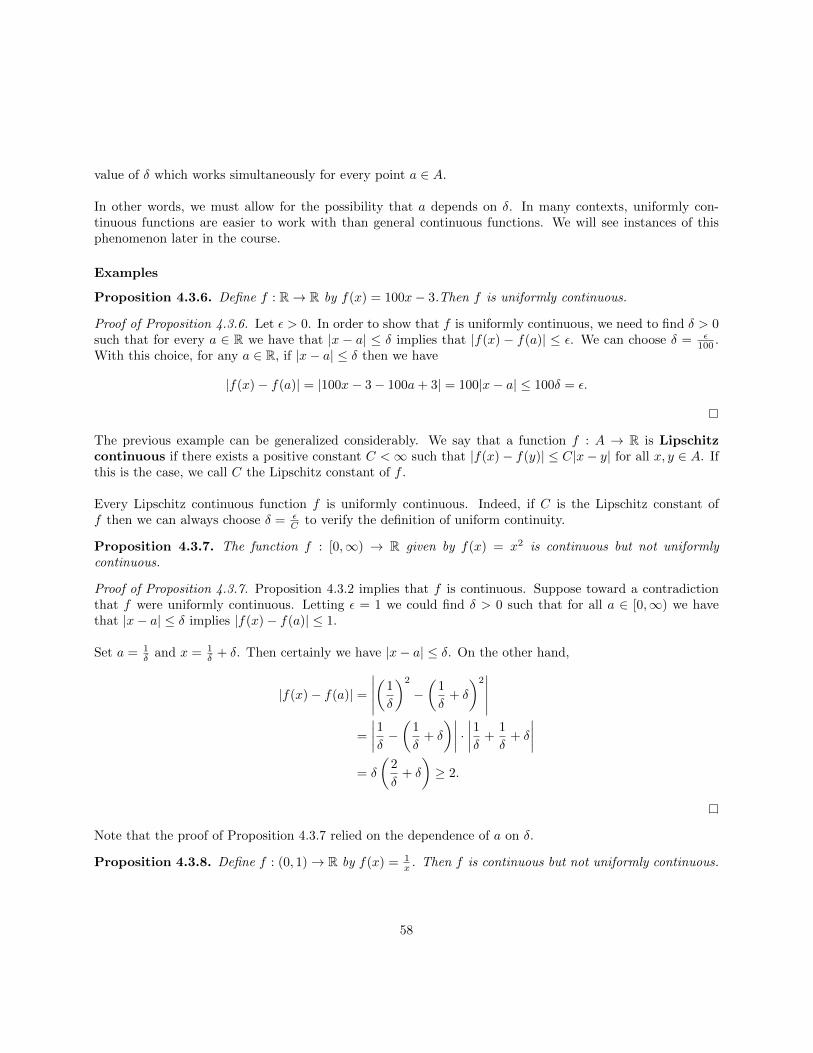
value of δ which works simultaneously for every point a ∈ A.

In other words, we must allow for the possibility that a depends on δ. In many contexts, uniformly con-tinuous functions are easier to work with than general continuous functions. We will see instances of thisphenomenon later in the course.

Examples

Proposition 4.3.6. Define f : R→ R by f(x) = 100x− 3.Then f is uniformly continuous.

Proof of Proposition 4.3.6. Let ε > 0. In order to show that f is uniformly continuous, we need to find δ > 0such that for every a ∈ R we have that |x − a| ≤ δ implies that |f(x) − f(a)| ≤ ε. We can choose δ = ε

100 .With this choice, for any a ∈ R, if |x− a| ≤ δ then we have

|f(x)− f(a)| = |100x− 3− 100a+ 3| = 100|x− a| ≤ 100δ = ε.

The previous example can be generalized considerably. We say that a function f : A → R is Lipschitzcontinuous if there exists a positive constant C <∞ such that |f(x)− f(y)| ≤ C|x− y| for all x, y ∈ A. Ifthis is the case, we call C the Lipschitz constant of f .

Every Lipschitz continuous function f is uniformly continuous. Indeed, if C is the Lipschitz constant off then we can always choose δ = ε

C to verify the definition of uniform continuity.

Proposition 4.3.7. The function f : [0,∞) → R given by f(x) = x2 is continuous but not uniformlycontinuous.

Proof of Proposition 4.3.7. Proposition 4.3.2 implies that f is continuous. Suppose toward a contradictionthat f were uniformly continuous. Letting ε = 1 we could find δ > 0 such that for all a ∈ [0,∞) we havethat |x− a| ≤ δ implies |f(x)− f(a)| ≤ 1.

Set a = 1δ and x = 1

δ + δ. Then certainly we have |x− a| ≤ δ. On the other hand,

|f(x)− f(a)| =

∣∣∣∣∣(

1

δ

)2

−(

1

δ+ δ

)2∣∣∣∣∣

=

∣∣∣∣1δ −(

1

δ+ δ

)∣∣∣∣ · ∣∣∣∣1δ +1

δ+ δ

∣∣∣∣= δ

(2

δ+ δ

)≥ 2.

Note that the proof of Proposition 4.3.7 relied on the dependence of a on δ.

Proposition 4.3.8. Define f : (0, 1)→ R by f(x) = 1x . Then f is continuous but not uniformly continuous.

58

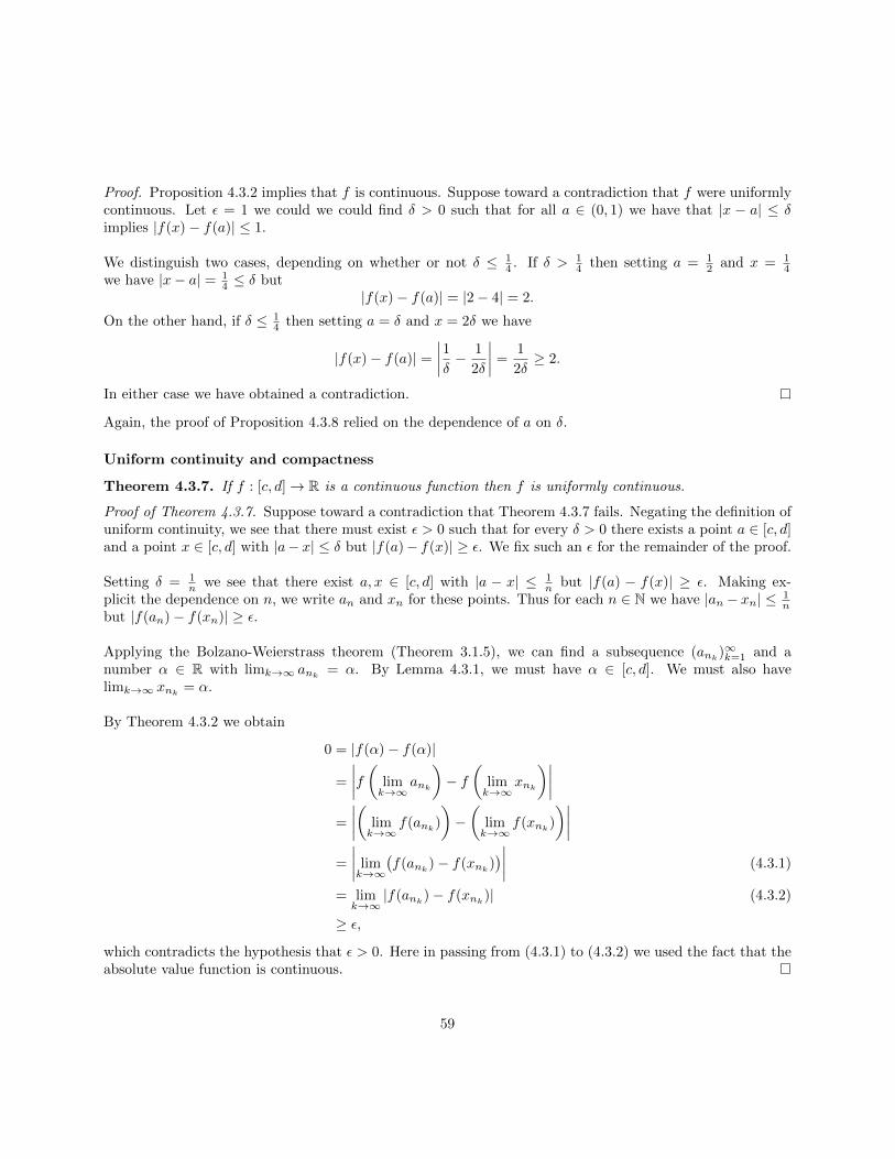
Proof. Proposition 4.3.2 implies that f is continuous. Suppose toward a contradiction that f were uniformlycontinuous. Let ε = 1 we could we could find δ > 0 such that for all a ∈ (0, 1) we have that |x − a| ≤ δimplies |f(x)− f(a)| ≤ 1.

We distinguish two cases, depending on whether or not δ ≤ 14 . If δ > 1

4 then setting a = 12 and x = 1

4we have |x− a| = 1

4 ≤ δ but|f(x)− f(a)| = |2− 4| = 2.

On the other hand, if δ ≤ 14 then setting a = δ and x = 2δ we have

|f(x)− f(a)| =∣∣∣∣1δ − 1

2δ

∣∣∣∣ =1

2δ≥ 2.

In either case we have obtained a contradiction.

Again, the proof of Proposition 4.3.8 relied on the dependence of a on δ.

Uniform continuity and compactness

Theorem 4.3.7. If f : [c, d]→ R is a continuous function then f is uniformly continuous.

Proof of Theorem 4.3.7. Suppose toward a contradiction that Theorem 4.3.7 fails. Negating the definition ofuniform continuity, we see that there must exist ε > 0 such that for every δ > 0 there exists a point a ∈ [c, d]and a point x ∈ [c, d] with |a− x| ≤ δ but |f(a)− f(x)| ≥ ε. We fix such an ε for the remainder of the proof.

Setting δ = 1n we see that there exist a, x ∈ [c, d] with |a − x| ≤ 1

n but |f(a) − f(x)| ≥ ε. Making ex-plicit the dependence on n, we write an and xn for these points. Thus for each n ∈ N we have |an − xn| ≤ 1

nbut |f(an)− f(xn)| ≥ ε.

Applying the Bolzano-Weierstrass theorem (Theorem 3.1.5), we can find a subsequence (ank)∞k=1 and a

number α ∈ R with limk→∞ ank= α. By Lemma 4.3.1, we must have α ∈ [c, d]. We must also have

limk→∞ xnk= α.

By Theorem 4.3.2 we obtain

0 = |f(α)− f(α)|

=

∣∣∣∣f ( limk→∞

ank

)− f

(limk→∞

xnk

)∣∣∣∣=

∣∣∣∣( limk→∞

f(ank)

)−(

limk→∞

f(xnk)

)∣∣∣∣=

∣∣∣∣ limk→∞

(f(ank

)− f(xnk))∣∣∣∣ (4.3.1)

= limk→∞

|f(ank)− f(xnk

)| (4.3.2)

≥ ε,

which contradicts the hypothesis that ε > 0. Here in passing from (4.3.1) to (4.3.2) we used the fact that theabsolute value function is continuous.

59

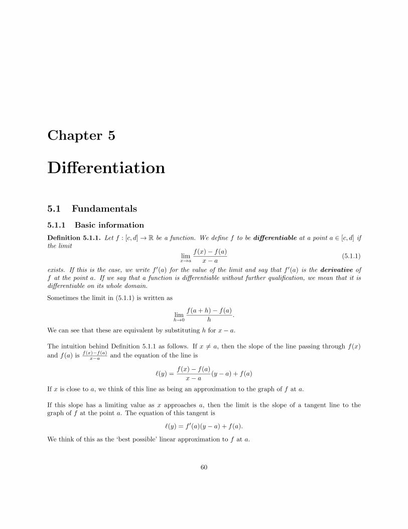
Chapter 5

Differentiation

5.1 Fundamentals

5.1.1 Basic information

Definition 5.1.1. Let f : [c, d]→ R be a function. We define f to be differentiable at a point a ∈ [c, d] ifthe limit

limx→a

f(x)− f(a)

x− a(5.1.1)

exists. If this is the case, we write f ′(a) for the value of the limit and say that f ′(a) is the derivative off at the point a. If we say that a function is differentiable without further qualification, we mean that it isdifferentiable on its whole domain.

Sometimes the limit in (5.1.1) is written as

limh→0

f(a+ h)− f(a)

h.

We can see that these are equivalent by substituting h for x− a.

The intuition behind Definition 5.1.1 as follows. If x 6= a, then the slope of the line passing through f(x)

and f(a) is f(x)−f(a)x−a and the equation of the line is

`(y) =f(x)− f(a)

x− a(y − a) + f(a)

If x is close to a, we think of this line as being an approximation to the graph of f at a.

If this slope has a limiting value as x approaches a, then the limit is the slope of a tangent line to thegraph of f at the point a. The equation of this tangent is

`(y) = f ′(a)(y − a) + f(a).

We think of this as the ‘best possible’ linear approximation to f at a.

60

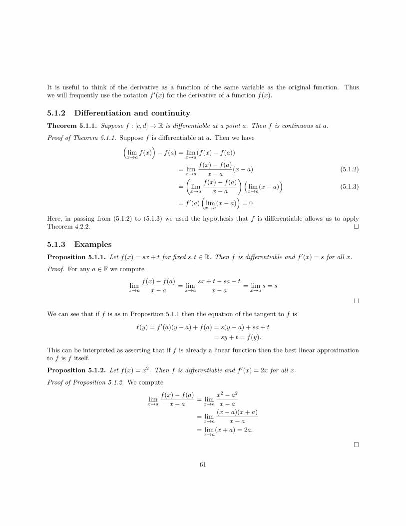
It is useful to think of the derivative as a function of the same variable as the original function. Thuswe will frequently use the notation f ′(x) for the derivative of a function f(x).

5.1.2 Differentiation and continuity

Theorem 5.1.1. Suppose f : [c, d]→ R is differentiable at a point a. Then f is continuous at a.

Proof of Theorem 5.1.1. Suppose f is differentiable at a. Then we have(limx→a

f(x))− f(a) = lim

x→a(f(x)− f(a))

= limx→a

f(x)− f(a)

x− a(x− a) (5.1.2)

=

(limx→a

f(x)− f(a)

x− a

)(limx→a

(x− a))

(5.1.3)

= f ′(a)(

limx→a

(x− a))

= 0

Here, in passing from (5.1.2) to (5.1.3) we used the hypothesis that f is differentiable allows us to applyTheorem 4.2.2.

5.1.3 Examples

Proposition 5.1.1. Let f(x) = sx+ t for fixed s, t ∈ R. Then f is differentiable and f ′(x) = s for all x.

Proof. For any a ∈ F we compute

limx→a

f(x)− f(a)

x− a= limx→a

sx+ t− sa− tx− a

= limx→a

s = s

We can see that if f is as in Proposition 5.1.1 then the equation of the tangent to f is

`(y) = f ′(a)(y − a) + f(a) = s(y − a) + sa+ t

= sy + t = f(y).

This can be interpreted as asserting that if f is already a linear function then the best linear approximationto f is f itself.

Proposition 5.1.2. Let f(x) = x2. Then f is differentiable and f ′(x) = 2x for all x.

Proof of Proposition 5.1.2. We compute

limx→a

f(x)− f(a)

x− a= limx→a

x2 − a2

x− a

= limx→a

(x− a)(x+ a)

x− a= limx→a

(x+ a) = 2a.

61

Theorem 5.1.1 implies that any discontinuous function is not differentiable. However, the following exampleshows that are continuous functions which are not differentiable.

Proposition 5.1.3. Let f(x) = |x|. Then f is not differentiable at 0.

Proof of Proposition 5.1.3. For x 6= 0 we have

f(x)− f(0)

x− 0=|x|x

=

{1 if x > 0

−1 if x < 0

Proposition 4.2.4 shows this limit does not exist as x→ 0.

5.1.4 Rules for taking derivatives

Arithmetic rules

Theorem 5.1.2. Suppose f and g are functions which are differentiable at a point a.

• (constant rule) If α ∈ R then (αf)′(a) = αf ′(a).

• (sum rule) We have (f + g)′(a) = f ′(a) + g′(a).

• (product rule) We have (fg)′(a) = f ′(a)g(a) + f(a)g′(a).

• (quotient rule) If g(a) 6= 0 then (f

g

)′(a) =

f ′(a)g(a)− f(a)g′(a)

g(a)2.

Implicit in these statements in Theorem 5.1.2 is that the assumptions imply all of the functions above aredifferentiable at a.

Proof of Theorem 5.1.2. We will prove the product rule and the quotient rule, as the proofs of the first tworules are straightforward.

Proof of product rule Write h = fg. We compute

limx→a

h(x)− h(a)

x− a= limx→a

f(x)g(x)− f(a)g(a)

x− a

= limx→a

f(x)g(x)− f(a)g(x) + f(a)g(x)− f(a)g(a)

x− a

=

(limx→a

f(x)g(x)− f(a)g(x)

x− a

)+

(limx→a

f(a)g(x)− f(a)g(a)

x− a

)=

(limx→a

f(x)− f(a)

x− ag(x)

)+ f(a)

(limx→a

g(x)− g(a)

x− a

)=

(limx→a

f(x)− f(a)

x− a

)(limx→a

g(x))

+ f(a)g′(a) (5.1.4)

= f ′(a)g(a) + f(a)g′(a) (5.1.5)

Here in passing from (5.1.4) to (5.1.5) we used the fact that since g is differentiable at a it must be continuousat a and therefore limx→a g(x) = g(a).

62

Proof of quotient rule Now, suppose h = fg and assume that g(a) 6= 0. Since g is continuous at a, this

implies that for x sufficiently close to a we have g(x) 6= 0. Therefore we are to free to divide by g(x) in ourcalculation of limits at a. We have

limx→a

h(x)− h(a)

x− a= limx→a

1

x− a

(f(x)

g(x)− f(a)

g(a)

)= limx→a

f(x)g(a)− f(a)g(x)

g(x)g(a)(x− a)

= limx→a

f(x)g(a)− f(a)g(a) + f(a)g(a)− f(a)g(x)

g(x)g(a)(x− a)

= limx→a

1

g(x)g(a)

(g(a)

f(x)− f(a)

x− a+ f(a)

g(a)− g(x)

x− a

)=

(limx→a

1

g(x)g(a)

)(g(a) lim

x→a

f(x)− f(a)

x− a− f(a) lim

x→a

g(x)− g(a)

x− a

)(5.1.6)

=f ′(a)g(a)− f(a)g′(a)

g(a)2(5.1.7)

Here in passing from (5.1.6) to (5.1.7) we used the fact that g is continuous at a to conclude that

limx→a

1

g(x)g(a)=

1

g(a)2

Derivatives of polynomials

Using the product rule, we can compute the derivative of any polynomial. We first compute the derivativesof monomials.

Proposition 5.1.4. Let n ∈ N and let mn(x) = xn. Then m′n(x) = nxn−1.

Proof of Proposition 5.1.4. We establish Proposition 5.1.4 by induction on n. Let P (n) be the statementthat m′n(x) = nxn−1. We have seen in Proposition 5.1.1 that P (1) is true.

Suppose we know that P (n) is true. We compute

m′n+1(x) = (mnm1)′(x) = m′n(x)m1(x) +m′1(x)mn(x)

= nxn−1 · x+ xn = (n+ 1)xn.

Therefore P (n+ 1) holds and by induction we see that P (n) holds for all n.

Combining Proposition 5.1.4 with the sum and constant rules we see that if p(x) =∑kn=0 cnx

n then

p′(x) =

k∑n=0

ncnxn−1 =

k−1∑n=0

(n+ 1)cn+1xn.

63

Chain rule

We now state the rule for how differentiation interacts with composition of functions.

Theorem 5.1.3 (Chain rule). Let f : [c, d] → R and g : [s, t] → R be functions such that f(x) ∈ [s, t] forall x ∈ [c, d]. Suppose that f is differentiable at a ∈ [c, d] and g is differentiable at f(a). Then g ◦ f isdifferentiable at a and (g ◦ f)′(a) = g′(f(a))f ′(a).

The proof of Theorem 5.1.3 will rely on the following lemma.

Lemma 5.1.1. A function f : [c, d] → R is differentiable at a ∈ [c, d] if and only if there exists a functionφ : [c, d]→ R which is continuous at a such that f(x)− f(a) = φ(x)(x− a) for all x ∈ [c, d]. In this case, wehave f ′(a) = φ(a).

Proof of Lemma 5.1.1. Suppose first that f is differentiable at a. Then we can define

φ(x) =

{f(x)−f(a)

x−a if x 6= a

f ′(a) if x = a.

The continuity of φ at a follows from the differentiability of f .

Suppose now that there exists a function φ as in the statement of the lemma. For x 6= a we can divideby x− a to obtain

limx→a

f(x)− f(a)

x− a= limx→a

φ(x) = φ(a)

since φ is continuous at a.

We now establish Theorem 5.1.3.

Proof of Theorem 5.1.3. Since f is differentiable at a, there exists a function φ : [c, d] → R which is con-tinuous at a with φ(a) = f ′(a) and such that f(x) − f(a) = φ(x)(x − a). Since g is differentiable at f(a),there exists a function ψ : [s, t] → R which is continuous at f(a) with ψ(f(a)) = g′(a) and such thatg(x)− g(a) = ψ(x)(x− a).

We computeg(f(x))− g(f(a)) = ψ(f(x))(f(x)− f(a)) = ψ(f(x))φ(x)(x− a).

If x 6= a we can divide by x− a to obtain

limx→a

g(f(x))− g(f(a))

x− a= limx→a

ψ(f(x))φ(x)

= ψ(f(a))φ(a) = g′(f(a))f ′(a).

5.2 Essential theorems about derivatives

In Section 5.2 we establish three essential theorems about derivatives. Each of these theorems will build onthe previous one.

64

5.2.1 Interior extremum theorem

Definition 5.2.1. If f : [c, d]→ R is a function, we say that f has a relative maximum at a point a ∈ [c, d]if there exists ε > 0 such that |x− a| ≤ ε implies f(a) ≥ f(x). We say that f has a relative minimum at aif the previous statement holds with the final inequality reversed. We say that f has a relative extremumat a if it has a relative maximum or a relative minimum at a.

Theorem 5.2.1. Suppose f : [c, d] → R is differentiable and that f has a relative extremum at a point asuch that c < a < d. Then f ′(a) = 0.

Proof of Theorem 5.2.1. We prove the case when f has a relative maximum at a. The case when f has arelative minumum at a can be established by applying the maximum case to −f .

Assume f has a relative maximum at a ∈ (c, d) and let ε > 0 be such that |x − a| ≤ ε implies f(a) ≥ f(x).Suppose toward a contradiction that f ′(a) > 0. Then there exists δ > 0 such that |x− a| ≤ δ implies∣∣∣∣f(x)− f(a)

x− a− f ′(a)

∣∣∣∣ ≤ f ′(a)

2.

In particular, we havef(x)− f(a)

x− a≥ f ′(a)

2.

Since a ∈ (c, d) there exists x ∈ (c, d) with

a < x < min(d, a+ ε, a+ δ).

Then

f(x)− f(a) ≥ f ′(a)(x− a)

2> 0,

contradicting the hypothesis that f has a relative maximum at a.

The possibility that f ′(a) < 0 can be excluded using a parallel argument.

5.2.2 Rolle’s theorem

Theorem 5.2.2 (Rolle’s theorem). Suppose c < d and suppose that f : [c, d] → R is differentiable withf(c) = f(d). Then there exists a ∈ (c, d) such that f ′(a) = 0.

Proof of Theorem 5.2.2. By replacing f with f − f(c), we may assume without loss of generality thatf(c) = f(d) = 0. If f is identically 0, then f ′ is also identically 0 so the theorem is true in this case.Thus we may assume that f is not identically 0.

By replacing f with −f , we may assume that f(b) > 0 for some b ∈ (c, d). Since f is continuous, theextreme value theorem implies that there exists a ∈ [c, d] such that f(a) = supc≤x≤d f(x). We havef(a) ≥ f(b) > 0 = f(c) = f(d), so that a ∈ (c, d). Then the interior extemum theorem implies thatf ′(a) = 0.

65

5.2.3 Mean value theorem

Theorem 5.2.3 (Mean value theorem). Suppose c < d and suppose that f : [c, d] → R is differentiable.Then there exists a ∈ [c, d] such that

f ′(a) =f(d)− f(c)

c− dProof of Theorem 5.2.3. Define

g(x) = f(x)− f(c)− f(d)− f(c)

d− c(x− c).

We can compute that g(c) = g(d) = 0. By Rolle’s theorem (Theorem 5.2.2), there exists a point a ∈ [c.d]such that g′(a) = 0. We have

g′(a) = f ′(a)− f(d)− f(c)

d− cwhich establishes Theorem 5.2.3.

66

Chapter 6

Integration

6.1 Fundamental definitions

Definition 6.1.1. Let [a, b] be a closed interval of finite length. A partition of [a, b] is a strictly increasingfinite list of points x0 < x1 < · · · < xn−1 < xn in [a, b] such that x0 = a and xn = b. The norm of apartition is the positive number

max(x1 − x0, x2 − x1, . . . , xn − xn−1)

We denote the norm of a partition P by ||P||.

Definition 6.1.2. Given a partition P = {x0, . . . , xn} of [a, b], a set of tags for P is a list t1, . . . , tn ofreal numbers such that xk−1 ≤ tk ≤ xk for all k ∈ {1, . . . , n}. A tagged partition is a partition with adistinguished set of tags.

Definition 6.1.3. If P is a tagged partition of [a, b] and a function f : [a, b]→ R, the Riemann sum of fover P is denoted S(P, f) and is defined by

S(P, f) =

n∑k=1

f(tk)(xk − xk−1)

Definition 6.1.4. A function f : [a, b]→ R is integrable if there exists a real number α such that for everyε > 0 there exists δ > 0 such that if P is a partition of ]a, b] such that ||P|| ≤ δ then |S(P, f) − α| ≤ ε. Ifthis is the case we say that α is the integral of f and write

α =

∫ b

a

f(x) dx

6.2 Uniqueness of the integral

Theorem 6.2.1. The integral of an integrable function is unique.

67

Proof of Theorem 6.2.1. Let f : [a, b] → R be an integrable function and assume that α and β satisfy thecondition in Definition 6.1.4. Let ε > 0. We can find δ > 0 such that if P is a partition of [a, b] with ||P|| ≤ δthen |S(P, f)−α| ≤ ε

2 . Similarly, we can find δ′ > 0 such that if P is a partition of [a, b] with ||P|| ≤ δ′ then|S(P, f)− β| ≤ δ.

Let n ∈ N be such that b−an ≤ min(δ, δ′) and consider the partition

P =

{a, a+

b− an

, a+2(b− a)

n, . . . , a+

(n− 1)(b− a)

b, b

}We have ||P|| ≤ min(δ, δ′). Thus we can use the triangle inequality to obtain

|α− β| ≤ |α− S(P, f)|+ |S(P, f)− β| ≤ ε

2+ε

2= ε

6.3 Criteria for integrability

Theorem 6.3.1 (Cauchy criterion). A function f : [a, b] → R is integrable if and only if the followingcondition holds. For every ε > 0 there exists δ > 0 such that if P and Q are partitions of [a, b] withmax(||P||, ||Q||) ≤ δ then |S(P, f)− S(Q, f)| ≤ ε.

Proof of Theorem 6.3.1. We treat each implication separately.

Integrability implies Cauchy Assume that f is integrable and let ε > 0. Writing α for the integral off , we can find δ > 0 such that if P is a partition with ||P|| ≤ δ then we have |S(P, f)− α| ≤ ε

2 . Then if Qis another partition with ||Q|| ≤ δ we also have |S(Q, f)− α| ≤ δ. Using the triangle inequality we obtain

|S(P, f)− S(Q, f)| ≤ |S(P, f)− α|+ |α− S(Q, f)| ≤ ε

2+ε

2= ε

Cauchy implies integrability Assume that f satisfies the Cauchy criterion. For each n ∈ N we can findδn such that if P and Q are partitions with max(||P||, ||Q||) ≤ δn then |S(P, f) − S(Q, f)| ≤ 1

n . We mayassume without loss of generality that δn+1 ≤ δn.

For each n, let Pn be a partition with ||Pn|| ≤ δn. If m > n then since ||Pm|| ≤ δm ≤ δn we have|S(Pm, f) − S(Pn, f)| ≤ 1

n . This implies that (S(Pn, f))∞n=1 is a Cauchy sequence of real numbers. ByTheorem 3.1.6 this sequence is convergent. Let α = limn→∞ S(Pn, f).

Now, let ε > 0. We can find N ∈ N such that n ≥ N implies |S(Pn, f) − α| ≤ ε2 . We may assume

that 1N ≤

ε2 . Let Q be a partition with ||Q|| ≤ δn, so that

|S(Q, f)− S(Pn, f)| ≤ 1

n≤ 1

N≤ ε

2

Using the triangle inequality we have

|S(Q, f)− α| ≤ |S(Q, f)− S(Pn, f)|+ |S(Pn, f)− α| ≤ ε

2+ε

2= ε

68

Definition 6.3.1. Let f : [a, b]→ R be an integrable function and let P = {x0, . . . , xn} be a partition of [a, b].For each k ∈ {1, . . . , n} define uk = supxk−1≤x≤xk

f(x) and lk = infxk−1≤x≤xkf(x). The upper Riemann

sum of f over P is denoted U(P, f) and is defined by

U(P, f) =

n∑k=1

uk(xk − xk−1)

The lower Riemann sum of f over P is denoted L(P, f) and is defined by

L(P, f) =

n∑k=1

lk(xk − xk−1)

Theorem 6.3.2 (Max-min criterion). A function f : [a, b] → R is integrable if and only if for every ε > 0there exists δ > 0 such that if P is a partition of [a, b] with ||P|| ≤ δ then U(P, f)− L(P, f) ≤ ε.

Proof of Theorem 6.3.2. It is immediate that the Cauchy criterion in Theorem 6.3.1 implies the criterion inTheorem 6.3.2. We now show that the criterion in Theorem 6.3.2 implies the Cauchy criterion in Theorem6.3.1. Let ε > 0 and let δ > 0 be such that if P is a partition with ||P|| ≤ δ then U(P, f) − L(P, f) ≤ ε

2 .Let Q be another partition with ||Q|| ≤ δ. It follows directly from the definition that if S(P, f) is a Rie-mann sum with an arbitrary set of tags then U(P, f) ≥ S(P, f) ≥ L(P, f) and U(Q, f) ≥ S(Q, f) ≥ L(Q, f).

Now, letR be the common refinement of P andQ. This means thatR is the partition whose set of subintervalendpoints is the union of the set of P endpoints and Q endpoints. We have U(R, f) ≤ min(U(P, f), U(Q, f))and L(R, f) ≥ max(L(P, f), L(Q, f)). Therefore the intervals [L(P, f), U(P, f)] and [L(Q, f), U(Q, f)] mustoverlap. Since these intervals have length at most ε

2 we see that |S(P, f)− S(Q, f)| ≤ ε as required.

6.4 Integrability of continuous functions

Theorem 6.4.1. Let f : [a, b]→ R be a continuous function. Then f is integrable.

Proof of Theorem 6.4.1. Let ε > 0. By Theorem 4.3.7 there exists δ > 0 such that if |x − y| ≤ δ then|f(x) − f(y)| ≤ ε

b−a . Let P = {x0, . . . , xn} be a partition with ||P|| ≤ δ and for each k ∈ {1, . . . , n} let ukand lk be as Definition 6.3.1.

By the extreme value theorem (Theorem 4.3.6) there exist sk ∈ [xk−1, xk] and vk ∈ [xk−1, xk] such thatf(sk) = uk and f(vk) = lk. Since xk − xk−1 ≤ δ we have |sk − vk| ≤ δ and therefore uk − lk ≤ ε

b−a . Thus wecan estimate

U(P, f)− L(P, f) =

n∑k=1

uk(xk − xk−1)−n∑k=1

lk(xk − xk−1)

=

n∑k=1

(uk − lk)(xk − xk−1)

≤n∑k=1

ε

b− a(xk − xk−1)

69

=ε

b− a

n∑k=1

(xk − xk−1)

=ε

b− a(b− a)

= ε

Thus Theorem 6.3.2 implies that f is integrable.

6.5 First fundamental theorem

Theorem 6.5.1 (First fundamental theorem of calculus). Let f : [a, b]→ R be a continuous function. Definea function g : [a, b]→ R by

g(y) =

∫ y

a

f(x) dx

Then g′(y) = f(y) for all y ∈ [a, b]

Proof of Theorem 6.5.1. We have

g(y + h)− g(y)

h=

1

h

(∫ y+h

a

f(x) dx−∫ y

a

f(x) dx

)

=1

h

∫ y+h

y

f(x) dx

Let ε > 0. Since f is continuous, we can find δ > 0 such that if |y − x| ≤ δ then |f(x)− f(y)| ≤ ε. We have∣∣∣∣∣ 1h∫ y+h

y

f(x) dx− f(y)

∣∣∣∣∣ =

∣∣∣∣∣ 1h∫ y+h

y

f(x) dx− 1

h

∫ y+h

y

f(y) dy

∣∣∣∣∣=

∣∣∣∣∣ 1h∫ y+h

y

f(x)− f(y) dx

∣∣∣∣∣≤ 1

h

∫ y+h

y

|f(x)− f(y)| dx

≤ 1

h

∫ y+h

y

ε dx

= ε

6.6 Second fundamental theorem

Theorem 6.6.1 (Second fundamental theorem of calculus). Let f : [a, b]→ R be a continuous function. LetF : [a, b]→ R satisfy F ′(x) = f(x) for all x ∈ [a, b]. Then we have∫ b

a

f(x) dx = F (b)− F (a)

70

Proof of Theorem 6.6.1. Let ε > 0. By Theorem 4.3.7 there exists δ > 0 such that if |x − y| ≤ δ then|f(x)− f(y)| ≤ ε

b−a . Let P = {x0, . . . , xn} be a partition of [a, b] with ||P|| ≤ δ and let t1, . . . , tn be a set oftags for P.

By the mean value theorem (Theorem 5.2.3) for every k ∈ {1, . . . , n} there exists sk ∈ [xk−1, xk] suchthat

F (xk)− F (xk−1)

xk − xk−1= f(sk)

or equivalentlyF (xk)− F (xk−1) = f(sk)(xk − xk−1)

We have ∣∣∣∣∣n∑k=1

f(tk)(xk − xk−1)−n∑k=1

f(sk)(xk − xk−1)

∣∣∣∣∣ =

∣∣∣∣∣n∑k=1

(f(tk)− f(sk)(xk − xk−1)

∣∣∣∣∣≤

n∑k=1

|f(tk)− f(sk)|(xk − xk−1)

≤ ε

b− a

n∑k=1

(xk − xk−1)

= ε

On the other handn∑k=1

f(sk)(xk − xk−1) =

n∑k=1

(F (xk)− F (xk−1)) = F (b)− F (a)

Therefore |S(P, f)− (F (b)− F (b)| ≤ ε.

71

Department of MathematicsThe University of Texas at Austinpjburton@math.utexas.edu

72