Read: Chapter CONTENTS - Texas A&M Universitymechanics.tamu.edu/wp-content/uploads/2016/09/05_Egnval-Trans.pdf · Read: Chapter 6 1D Eigenvalue and Time-Dependent Problems • Eigenvalue

JN Reddy

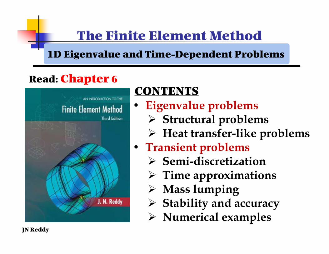
The Finite Element Method

Read: Chapter 6

1D Eigenvalue and Time-Dependent Problems

• Eigenvalue problems Structural problems Heat transfer-like problems

• Transient problems Semi-discretization Time approximations Mass lumping Stability and accuracy Numerical examples

CONTENTS

JN Reddy

INTRODUCTION

Equations of motion

Static problem (set all derivatives with respect to time

t to zero)

Construct FE model

Construct weak form

Semidiscretization(construct weak form in spatial

coordinates and semi-discrete FEM)

Full discretization (use time

approximations)

Eigenvalue problem (replace the solution with periodic or decaytype solution with respect to time t)

Construct FE model

Construct weak form

JN Reddy

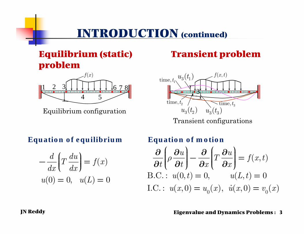
INTRODUCTION (continued)

( )f x

Equilibrium configuration

• • • • • • • •1 2 3

4 56 7 8

3u

( , )f x t

Transient configurations

3 1( )u t

• • • • • • • •

2time,t

1time,t

3time,t

3

3 2( )u t 3 3( )u t

r

0 0

( , )

B.C. : (0, ) 0, ( , ) 0

I.C. : ( , 0) ( ), ( , 0) ( )

u uT f x t

t t x xu t u L t

u x u x u x v x

æ ö æ ö¶ ¶ ¶ ¶ç ÷ ç ÷- =ç ÷ ç ÷ç ÷ ç ÷ç ÷ ç ÷¶ ¶ ¶ ¶è ø è ø= == =

( )

(0) 0, ( ) 0

d duT f x

dx dxu u L

æ öç ÷- =ç ÷ç ÷è ø= =

Eigenvalue and Dynamics Problems : 3

Equilibrium (static) problem

Transient problem

Equation of equilibrium Equation of motion

JN Reddy Eigenvalue and Dynamics Problems : 4

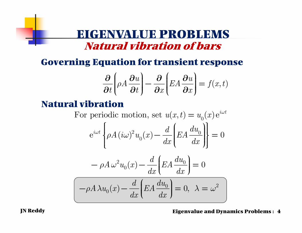
EIGENVALUE PROBLEMS

w

w

r

r w

0

2 00

( , )

For periodic motion, set ( , ) ( )e

e ( ) ( ) 0

i t

i t

u uA EA f x t

t t x x

u x t u x

dudA i u x EA

dx dx

æ ö æ ö¶ ¶ ¶ ¶ç ÷ ç ÷- =ç ÷ ç ÷ç ÷ ç ÷ç ÷ ç ÷¶ ¶ ¶ ¶è ø è ø

=ì üæ öï ïç ÷ï ïç ÷- =í ýç ÷ï ïç ÷è øï ïî þ

2 00

200

( ) 0

( ) 0,

dudA u x EA

dx dxdud

A u x EAdx dx

r w

r l l w

æ öç ÷- - =ç ÷ç ÷è øæ öç ÷- - = =ç ÷ç ÷è ø

Natural vibration of barsGoverning Equation for transient response

Natural vibration

JN Reddy Eigenvalue and Dynamics Problems : 5

t

t

g T x t T x

T TA kAt x x

dTdA T x kA

dx dx

0

00

0, ( , ) ( )e

0

e ( ) ( ) 0

l

l

r

r l

-

-

= =

æ ö¶ ¶ ¶ç ÷- =ç ÷ç ÷è ø¶ ¶ ¶ì üæ öï ïï ïç ÷- - =í ýç ÷ç ÷è øï ïï ïî þ

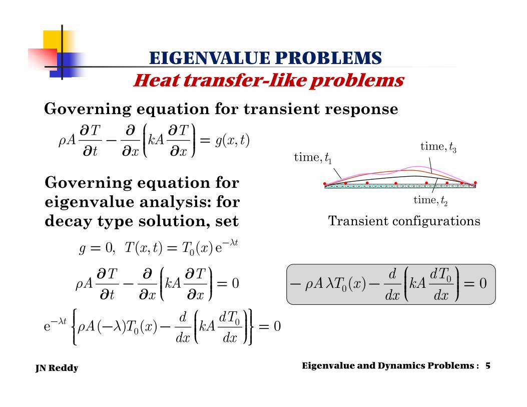
T TA kA g x tt x x

( , )ræ ö¶ ¶ ¶ç ÷- =ç ÷ç ÷è ø¶ ¶ ¶

Governing equation for transient response

00( ) 0

dTdA T x kA

dx dxr l

æ öç ÷- - =ç ÷ç ÷è ø

Governing equation for eigenvalue analysis: for decay type solution, set

EIGENVALUE PROBLEMS Heat transfer-like problems

Transient configurations

• • • • • • • •

t2time,

t1time,t3time,

JN Reddy

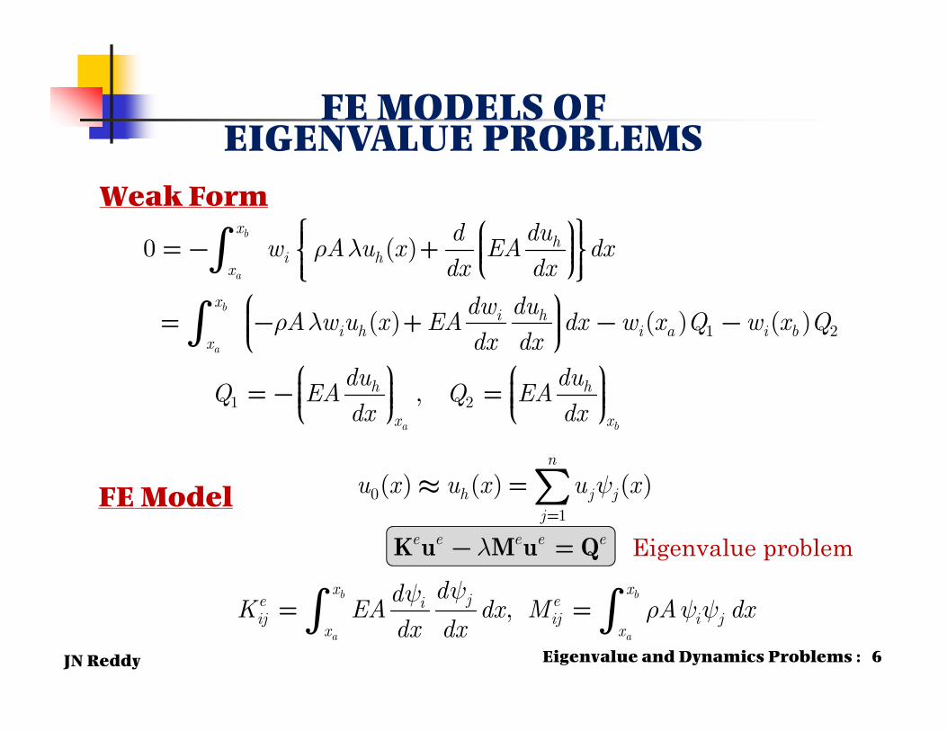
FE MODELS OF EIGENVALUE PROBLEMS

01

( ) ( ) ( )

,b b

a a

n

h j jj

e e e e e

x xje ei

ij ij i jx x

u x u x u x

ddK EA dx M A dx

dx dx

y

l

yyr y y

=

» =

- =

= =

å

ò ò

K u M u Q

FE Model

Weak Form

1 2

1 2

0 ( )

( ) ( ) ( )

,

b

a

b

a

a b

xh

i hx

xi h

i h i a i bx

h h

x x

dudw A u x EA dx

dx dx

dw duA w u x EA dx w x Q w x Q

dx dxdu du

Q EA Q EAdx dx

r l

r l

ì üæ öï ïï ïç ÷=- +í ýç ÷ç ÷è øï ïï ïî þæ öç ÷= - + - -ç ÷ç ÷è ø

æ ö æ öç ÷ ç ÷=- =ç ÷ ç ÷ç ÷ ç ÷è ø è ø

ò

ò


Eigenvalue problem

JN Reddy

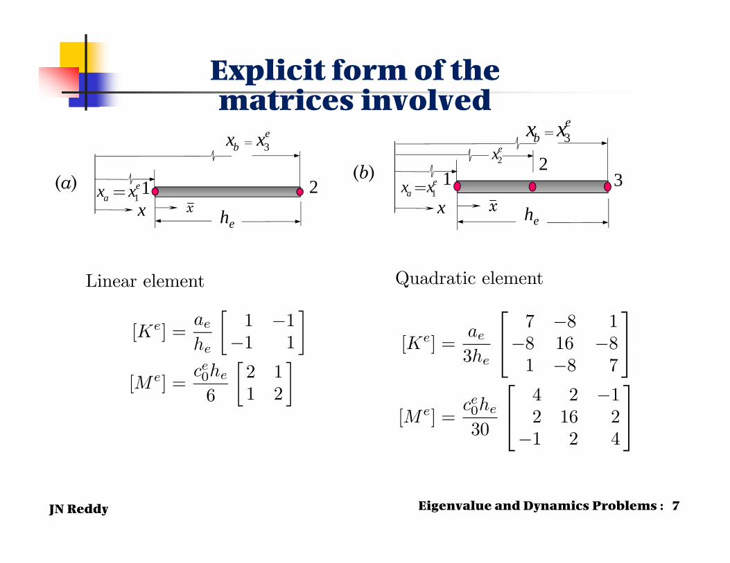
Linear element

[Ke] =aehe

1 −1−1 1

[Me] =ce0he6

2 11 2

Quadratic element

[Ke] =ae3he

⎡⎣ 7 −8 1−8 16 −81 −8 7

⎤⎦+[Me] =

ce0he30

⎡⎣ 4 2 −12 16 2−1 2 4

⎤⎦

Explicit form of the matrices involved

12

3x he

(b)

3e

bx x=ex2

1e

ax x=x

1 2x he

(a)

3e

bx x=

1e

ax x=x


JN Reddy

EXAMPLES: Axial vibrations of a bar (fundamental frequency)

Deformable bar

Problem 1

x

E, A k

L Deformable bar

Linear springProblem 2

1 1

2 2

1

2

21 1 2 161 1 1 2

u uEA ALu uL

QQ

wrì ü ì üé ù é ù- ï ï ï ïï ï ï ïê ú ê ú-í ý í ýê ú ê úï ï ï ï-ë û ë ûï ï ï ïî þ î þ

ì üï ïï ï= í ýï ïï ïî þ

0 0

0

22 2

2 306

orEA AL EuL L

rw w

ræ ö÷ç - = =÷ç ÷çè ø

1 1

2 2

1

2

21 1 2 161 1 1 2

u uEA ALu uL

QQ

wrì ü ì üé ù é ù- ï ï ï ïï ï ï ïê ú ê ú-í ý í ýê ú ê úï ï ï ï-ë û ë ûï ï ï ïî þ î þ

ì üï ïï ï= í ýï ïï ïî þ

0 0

2ku-

22

2

03

3( / A)or

EA ALk uL

E kLL

rw

wr

æ ö÷ç + - =÷ç ÷çè ø

+=


JN Reddy

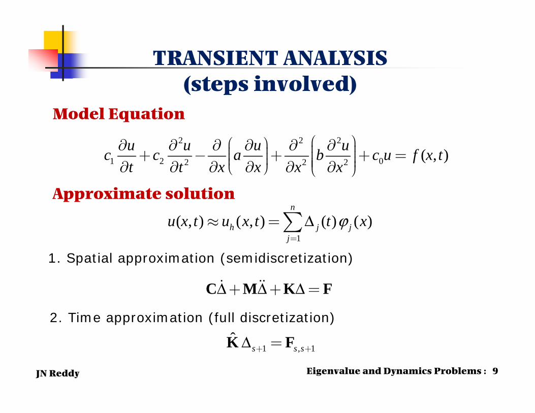
TRANSIENT ANALYSIS(steps involved)

2 2 2

1 2 02 2 2 ( , )u u u uc c a b c u f x tt t x x x x

æ öæ ö¶ ¶ ¶ ¶ ¶ ¶ ÷ç÷ç ÷+ - + + =÷ çç ÷÷ç ç ÷çè ø¶ ¶ ¶ ¶ ¶ ¶è ø

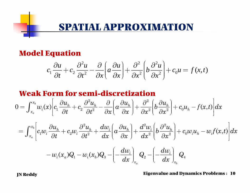
Model Equation

Approximate solution

1

( , ) ( , ) ( ) ( )n

h j jj

u x t u x t t xϕΔ=

» =å1. Spatial approximation (semidiscretization)

2. Time approximation (full discretization)

Δ Δ Δ+ + =C M K F

1 , 1K̂ Fs s sΔ + +=


JN Reddy

SPATIAL APPROXIMATION

2 2 2

1 2 02 2 2 ( , )u u u uc c a b c u f x tt t x x x x

æ öæ ö¶ ¶ ¶ ¶ ¶ ¶ ÷ç÷ç ÷+ - + + =÷ çç ÷÷ç ç ÷çè ø¶ ¶ ¶ ¶ ¶ ¶è ø

2 2

1 2 02 2 2

2 2 2

1 2 02 2 2

0 ( ) ( , )

( , )

b

a

b

a

xh h h h

i hx

xh h i h i h

i i i h ix

i

u u u uw x c c a b c u f x t dxt t x x x x

u u dw u d w uc w c w a b c w u w f x t dxt t dx x dx x

w

é ùæ ö æ ö¶ ¶ ¶ ¶¶ ¶÷ ÷ç çê ú= + - + + -÷ ÷ç ç÷ ÷ç çê úè ø è ø¶ ¶ ¶ ¶ ¶ ¶ë û

é ùæ öæ ö¶ ¶ ¶ ¶ ÷ç÷ê úç ÷= + + + + -÷ çç ÷÷ê úçç ÷çè ø¶ ¶ ¶ ¶è øë û

-

ò

ò

1 3 2 4( ) ( )a b

i ia i b

x x

dw dwx Q w x Q Q Qdx dx

æ ö æ ö÷ ÷ç ç- - - - -÷ ÷ç ç÷ ÷ç çè ø è ø

Model Equation

Weak Form for semi-discretization


JN Reddy

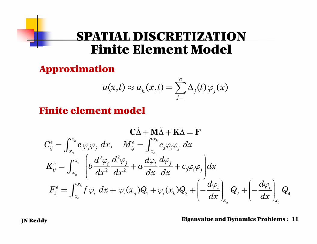
Approximation

Finite element model

1 2

22

02 2

1 3 2 4

,

( ) ( )

b b

a a

b

a

b

aa b

x xe eij i j ij i jx x

x j je i iij i jx

xe i ii i i a i bx

x x

C c dx M c dx

d dd dK b a c dxdx dx dx dx

d dF f dx x Q x Q Q Qdx dx

jj jj

j jj jjj

j jj j j

Δ Δ Δ+ + == =

æ ö÷ç ÷ç= + + ÷ç ÷ç ÷çè øæ ö æ ö÷ ÷ç ç÷ ÷= + + + - + -ç ç÷ ÷ç ç÷ ÷ç çè ø è ø

ò ò

ò

ò

C M K F

SPATIAL DISCRETIZATIONFinite Element Model

1

( , ) ( , ) ( ) ( )n

h j jj

u x t u x t t xjΔ=

» =å


JN Reddy

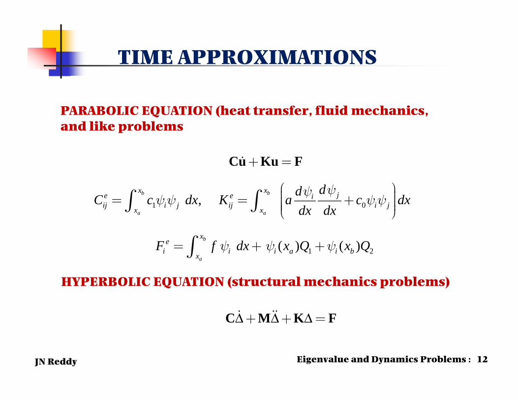
PARABOLIC EQUATION (heat transfer, fluid mechanics, and like problems

1 0

1 2

,

( ) ( )

yyyy yy

y y y

+ =

æ ö÷ç ÷= = +ç ÷ç ÷çè ø

= + +

ò ò

ò

Cu Ku F

b b

a a

b

a

x x je e iij i j ij i jx x

xe

i i i a i bx

ddC c dx K a c dxdx dx

F f dx x Q x Q

TIME APPROXIMATIONS

HYPERBOLIC EQUATION (structural mechanics problems)

C M K FΔ Δ Δ+ + =


JN Reddy

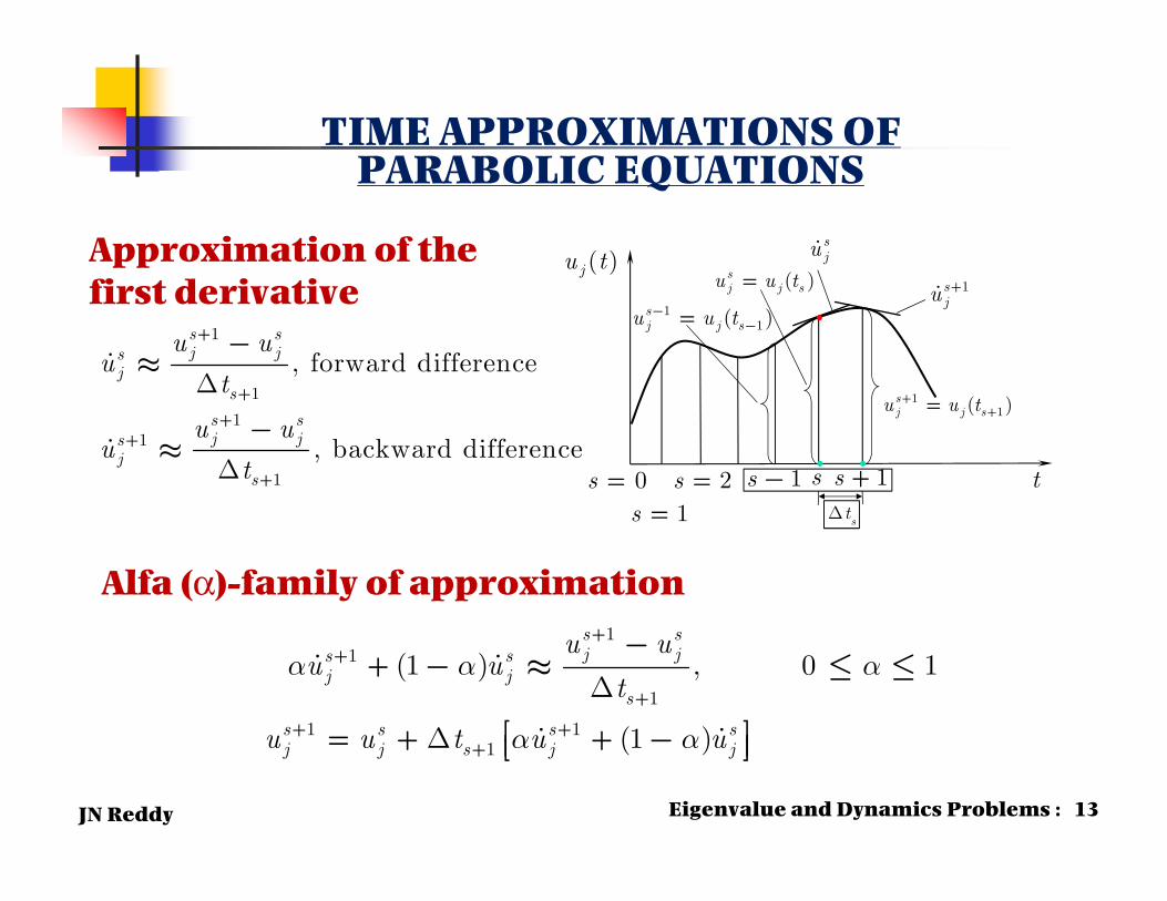
TIME APPROXIMATIONS OF PARABOLIC EQUATIONS

D

D

1

1

11

1

, forward difference

, backward difference

s sj js

js

s sj js

js

u uu

t

u uu

t

+

++

+

+

-»

-»

Approximation of thefirst derivative

a a a

a a

D

D

11

1

1 11

(1 ) , 0 1

(1 )

s sj js s

j js

s s s sj j s j j

u uu u

t

u u t u u

++

+

+ ++

-+ - » £ £

é ù= + + -ê úë û

Alfa (α)-family of approximation


11( )s

j j su u t--=

( )sj j su u t=

11( )s

j j su u t++=

stD

1sju+

0s =1s =

2s = 1s - s 1s +

( )ju t

t

•

• •

sju

JN Reddy

TIME APPROXIMATIONS (Parabolic)

Cu Ku F Cu K u F Cu K u F

u u u u

Cu Cu Cu Cu

s s s ss s s s

s s s ss

s s s ss

t T

t

t

a a

a a

D

D

1 11 1

1 11

1 11

, 0 ,

(1 )

(1 )

+ ++ +

+ ++

+ ++

+ = < < + = + =

é ù= + + -ê úë ûé ù= + + -ê úë û

Alfa-family of approximation (Parabolic equation)

Cu F K us s ss

1 1 11 + + +

+= -

( ) ( ) C K u C K u

F F

s ss s s s

s ss

t t

t

a a

a a

D D

D

11 1

11

(1 )

(1 )

++ +

++

+ = - -

é ù+ + -ê úë û1 1

1

1 1 1

1 11 1 1

ˆ ˆ

ˆ ,

ˆ (1 ) (1 )

s ss

s s s

s s s ss s s

where

t

t t

a

a a a

D

D D

+ ++

+ + +

+ ++ + +

=

= +

é ù é ù= - + + + -ê ú ê úë û ë û

K u F

K K C

F K C u F F

Cu F K us s ss = -


JN Reddy

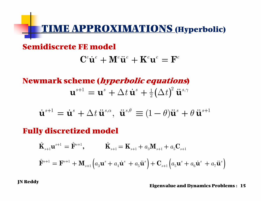
C u M u K u Fe e e e e e e+ + =

( )u u u u

u u u u u u

s s s s

s s s s s s

t t

t

g

a q q q

D D

D

21 ,12

1 , , 1, (1 )

+

+ +

= + +

= + º - +

Semidiscrete FE model

Newmark scheme (hyperbolic equations)

( ) ( )

K u F , K K M C

F F M u u u C u u u

s ss s s s s

s s s s s s s ss s

a a

a a a a a a

1 11 1 1 3 1 5 1

1 11 3 4 5 1 5 6 7

ˆ ˆ ˆ

ˆ

+ ++ + + + +

+ ++ +

= = + +

= + + + + + +

Fully discretized model

TIME APPROXIMATIONS (Hyperbolic)


JN Reddy

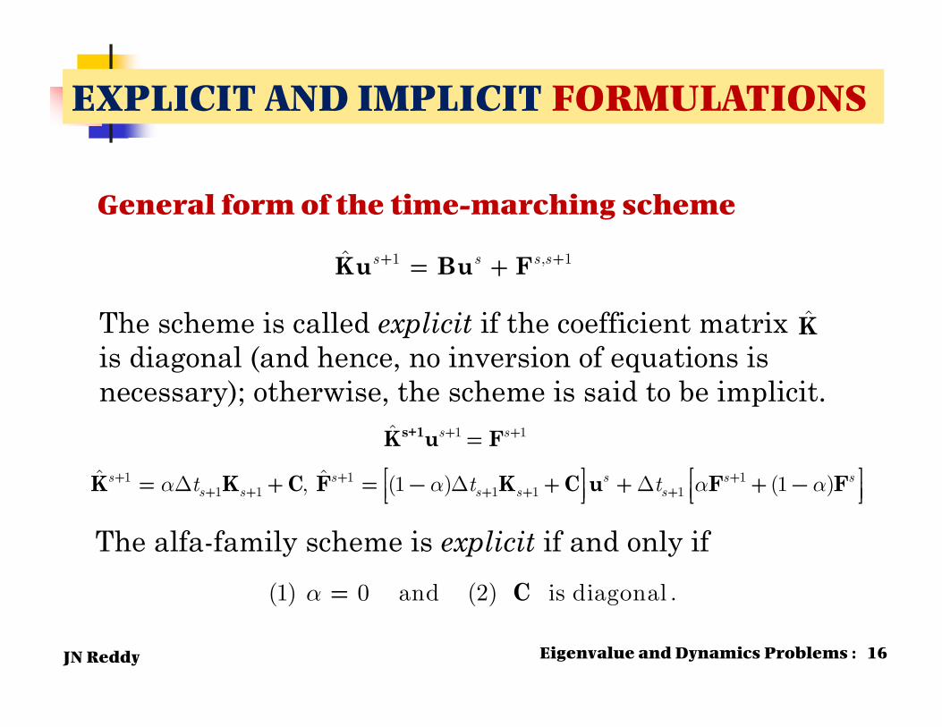
General form of the time-marching scheme

The scheme is called explicit if the coefficient matrix is diagonal (and hence, no inversion of equations is necessary); otherwise, the scheme is said to be implicit.

s+1K u F

K K C F K C u F FD D D

1 1

1 1 11 1 1 1 1

ˆ

ˆ ˆ, (1 ) (1 )

s s

s s s s ss s s s st t ta a a a

+ +

+ + ++ + + + +

=

é ù é ù= + = - + + + -ê ú ê úë û ë û

The alfa-family scheme is explicit if and only ifC(1) 0 and (2) is diagonal .a =

Ku Bu F1 , 1ˆ s s s s+ += +


K̂

EXPLICIT AND IMPLICIT FORMULATIONS

JN Reddy

ROW-SUM MASS LUMPING


For the Lagrange linear and quadratic elements we have

[Me]C =ρhe6

2 11 2

, [Me]C =ρhe30

⎡⎣ 4 2 −12 16 2−1 2 4

⎤⎦

[Me]L =ρhe2

1 00 1

, [Me]L =ρhe6

⎡⎣ 1 0 00 4 00 0 1

⎤⎦

6e eA hr

2e eA hr

6e eA hr

30e eA hr

JN Reddy

STABILITY OF APPROXIMATIONS

K u Ku F

u Au B

1 1 , 1

1 , 1

ˆ s s s s s

s s s s

+ + +

+ +

= +

= +

The scheme is called stable if the repeated solution of the above equation does not result in unbounded solution us+1. The necessary and sufficient condition for the above scheme to be stable is that the maximum eigenvalue of the coefficient matrix A is less than unity:

max 1Al £


JN Reddy

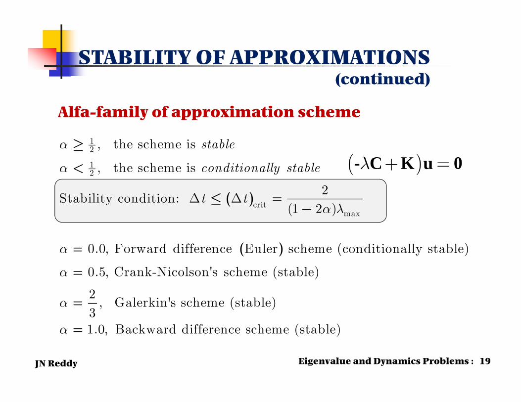
STABILITY OF APPROXIMATIONS (continued)

( )

( )

D D

12

12

critmax

, the scheme is

, the scheme is

2Stability condition:

(1 2 )

0.0, Forward difference Euler scheme (conditionally stable)

0.5, Crank-Nicolson's scheme (stabl

stable

conditionally stable

t t

a

a

a l

a

a

³

<

£ =-

=

= e)

2, Galerkin's scheme (stable)

31.0, Backward difference scheme (stable)

a

a

=

=

Alfa-family of approximation scheme


( )- C K u 0+ =l

JN Reddy

STABILITY OF APPROXIMATIONS (continued)

( )D Dcrit

max

13

2Stability condition:

( )

0.5, 2 0.5, Constant-average acceleration scheme (stable)

0.5, 2 , Linear acceleration scheme (conditionally stable)

1.5, 2 1.6, Galerkin's scheme (stab

t ta g l

a g b

a g b

a g b

£ =-

= = =

= = =

= = = le)

1.5, 2 2.0, Backward difference scheme (stable)a g b= = =

Newmark’s scheme for Structural Dynamics

gets smaller as the mesh is refined.( )crittD


( )- M K u 0+ =l

JN Reddy

0.0 1.0 2.0 3.0 4.0 5.0 6.0

Time, t

-2.50

-2.00

-1.50

-1.00

-0.50

0.00

0.50

1.00

1.50

2.00

Tem

pera

ture

,u(

1,t)

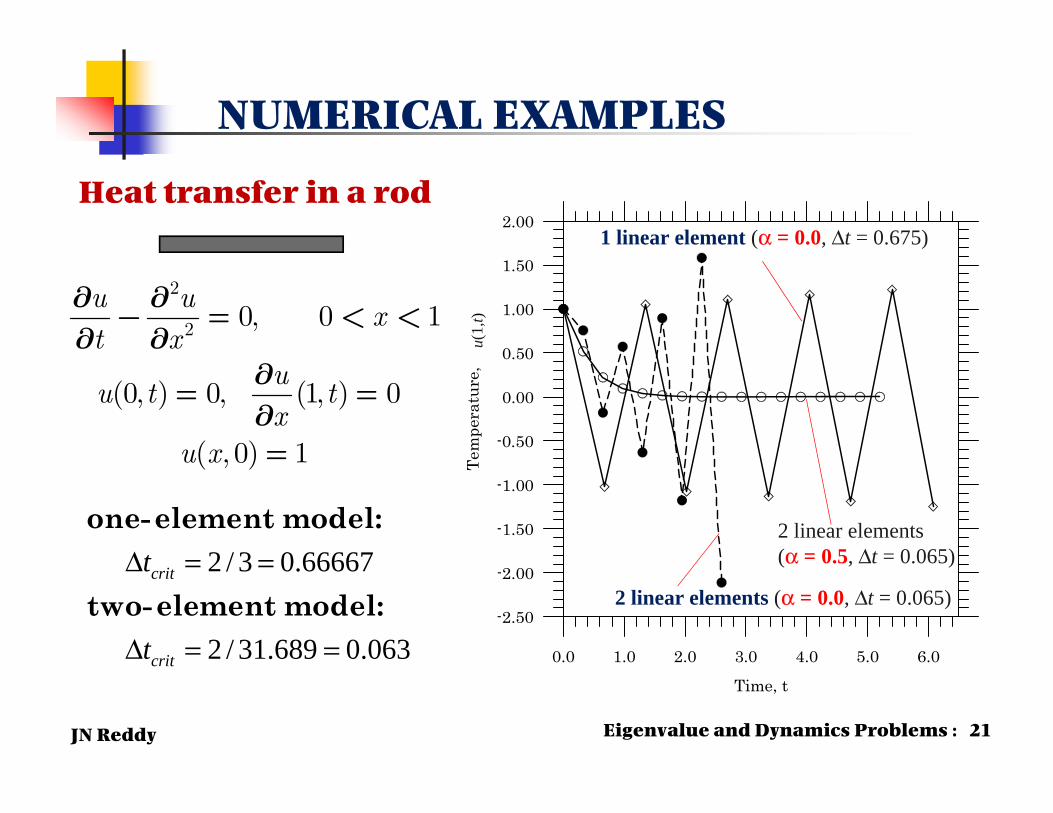
1 linear element (α = 0.0, Δt = 0.675)

2 linear elements (α = 0.0, Δt = 0.065)

2 linear elements (α = 0.5, Δt = 0.065)

NUMERICAL EXAMPLES

Heat transfer in a rod

2

2 0, 0 1

(0, ) 0, (1, ) 0

( , 0) 1

u ux

t xu

u t tx

u x

¶ ¶- = < <¶ ¶

¶= =¶=

2 / 3 0.66667

2 / 31.689 0.063

one-element model:

two-element model: crit

crit

t

t

Δ = =

Δ = =


JN Reddy

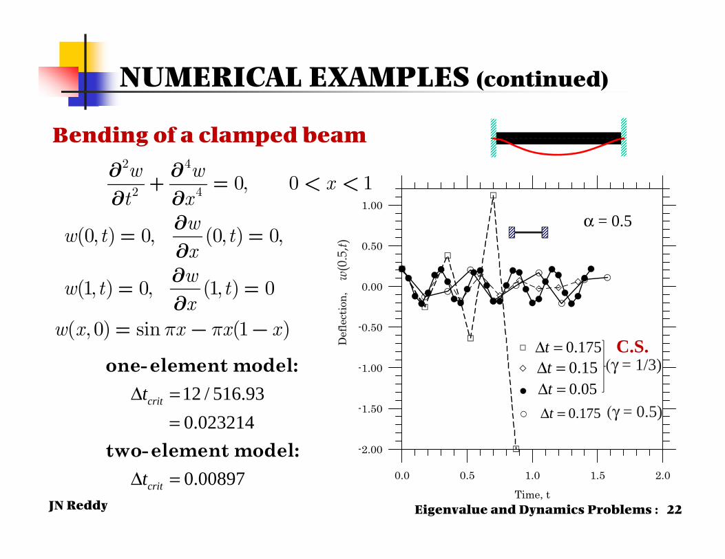
NUMERICAL EXAMPLES (continued)

Bending of a clamped beam

p p

2 4

2 4 0, 0 1

(0, ) 0, (0, ) 0,

(1, ) 0, (1, ) 0

( , 0) sin (1 )

w wx

t xw

w t txw

w t tx

w x x x x

¶ ¶+ = < <

¶ ¶¶= =¶¶= =¶

= - -

12 / 516.930.023214

0.00897

one-element model:

two-element model:

Δ ==

Δ =

crit

crit

t

tEigenvalue and Dynamics Problems : 22

w(0

.5,t)

0.0 0.5 1.0 1.5 2.0

Time, t

-2.00

-1.50

-1.00

-0.50

0.00

0.50

1.00

Def

lect

ion,

175.0=Δt15.0=Δt

175.0=Δt

α = 0.5

(γ = 0.5)

(γ = 1/3)05.0=Δt

C.S.

JN Reddy

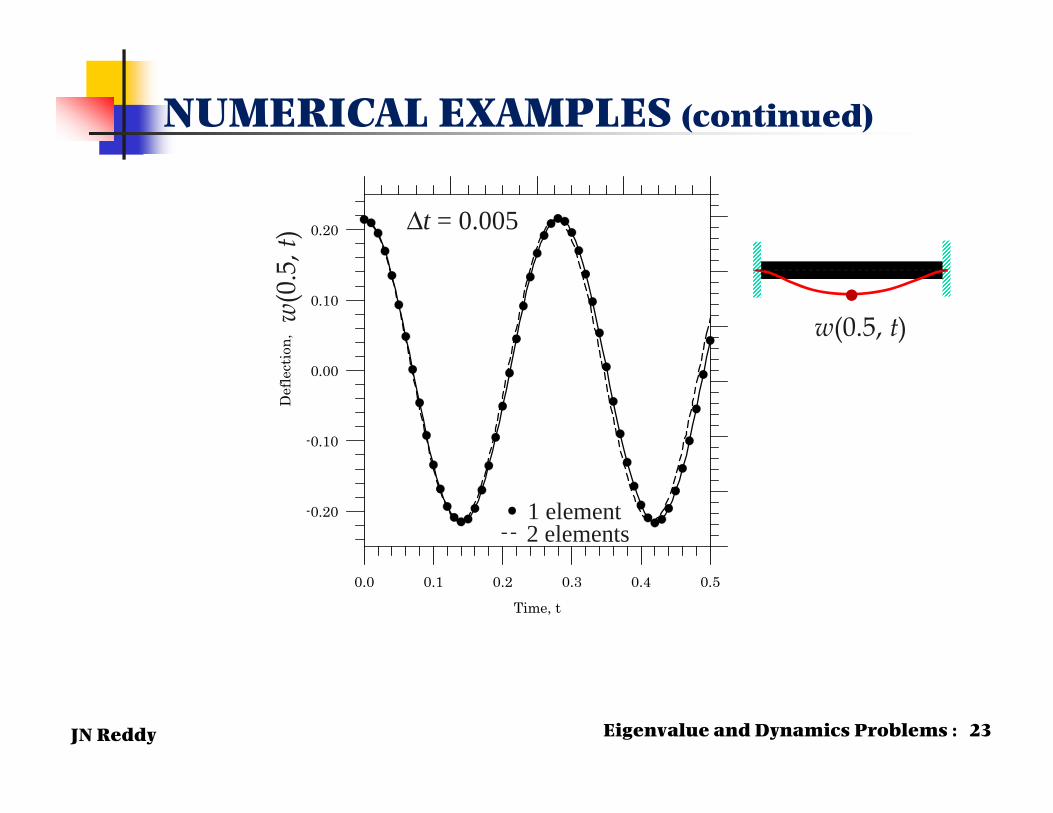
NUMERICAL EXAMPLES (continued)


0.0 0.1 0.2 0.3 0.4 0.5

Time, t

-0.20

-0.10

0.00

0.10

0.20

Def

lect

ion,

2 elements1 element

Δt = 0.005

w(0

.5, t

)w(0.5, t)●

JN Reddy 24

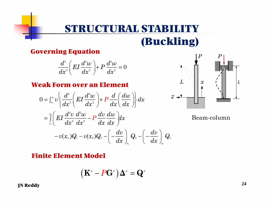
STRUCTURAL STABILITY (Buckling)

L x

P

z

Beam-column

P

L

Governing Equation2 2

2 2

2

20d d w d wEI P

dx dx dx

+ =

Weak Form over an Element2 2

2 2

2 2

2 2

1 3 2 4

0

( ) ( )

b

a

b

a

a b

x

x

x

x

a b

x x

d d d dwv EI dxdx dx dx dxd v d dv

P

dwEI dxdx dx dx dx

dv dvv x Q v x Q Q Qdx dx

w

w P

= +

= −

− − − − − −

Finite Element Model

( )e e e eP− =K G Δ Q

JN Reddy 2-D Problems: 25

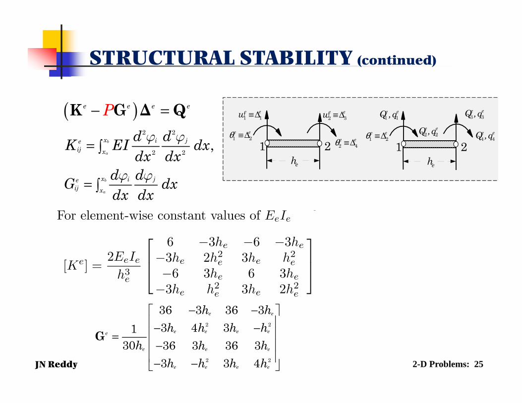
STRUCTURAL STABILITY (continued)

( )e e e eP− =K G Δ Q2 2

2 2,b

a

b

a

x i jeij x

x i jeij x

d dK EI dxdx dx

d dG dxdx dx

j j

j j

=

=

1 2ee21 Δ≡θ ee

42 Δ≡θ

eew 11 Δ≡ eew 32 Δ≡

eh

ee q,Q 22 ee q,Q 44

ee q,Q 11ee q,Q 33

1 2ee21 Δ≡θ

eh

For element-wise constant values of EeIe and qe:

[Ke] =2EeIeh3e

⎡⎢⎣6 −3he −6 −3he−3he 2h2e 3he h2e−6 3he 6 3he−3he h2e 3he 2h2e

⎤⎥⎦2 2

2 2

36 3 36 33 4 336 3 36 303 3 4

13

e e

e e e e

e

e e

e

e

e e e

h hh h h h

h hh h h h

h

− − − −

− −

=

−

G

JN Reddy 26

EXAMPLE: Buckling of a clamped-clamped beam

2 2 2 2

2 2 2

3

2

6 3 6 3 36 3 36 33 2 3 3 4 326 3 6 3 36 3 36 3

3 4 33

3 40

3

e e e e

e e e e e e e e

e e e e

e e e e e e e e

e e

h h h hh h h h h h h hEI

h h h hh h h h h h

hh

P

hh

− − − − − − − − − − − − − −

1

2

3

4

UUUU

(1)1

(1)2

(1)3

(1)4

QQQQ

=

1

2

3 3

4

00

0

UUU UU

=

(1) (1)1 1

(1) (1)2 2

(1)3

(1) (1)4 4

0

Q QQ QQQ Q

=

33 3 2

12 36 12 300 1030 36

EI EI L EIU PL L L L

P =

− = =

One-element (EBT) in half beam

Boundary conditions

Solution x

z

P

●

●

1

2

JN Reddy

SUMMARY

In this lecture the following topics were covered:

Transient and eigenvalue problems and their finite element formulations

Time-approximations of first-order andsecond-order equations

Explicit and implicit schemes, mass lumping, as well as stability of the schemes

Numerical examples to illustrate tostability and accuracy.

Buckling of beams


Documents

Read: Chapter CONTENTS - Texas A&M Universitymechanics.tamu.edu/wp-content/uploads/2016/09/05_Egnval-Trans.pdf · Read: Chapter 6 1D Eigenvalue and Time-Dependent Problems • Eigenvalue