Reactor Design

Andrew Rosen

May 11, 2014

Contents1 Mole Balances 3

1.1 The Mole Balance . . . . . . . . . . . . . . . . . . . . . . . . . . . . . . . . . . . . . . . . . . 31.2 Batch Reactor . . . . . . . . . . . . . . . . . . . . . . . . . . . . . . . . . . . . . . . . . . . . . 31.3 Continuous-Flow Reactors . . . . . . . . . . . . . . . . . . . . . . . . . . . . . . . . . . . . . . 4

1.3.1 Continuous-Stirred Tank Reactor (CSTR) . . . . . . . . . . . . . . . . . . . . . . . . . 41.3.2 Packed-Flow Reactor (Tubular) . . . . . . . . . . . . . . . . . . . . . . . . . . . . . . . 41.3.3 Packed-Bed Reactor (Tubular) . . . . . . . . . . . . . . . . . . . . . . . . . . . . . . . 4

2 Conversion and Reactor Sizing 52.1 Batch Reactor Design Equations . . . . . . . . . . . . . . . . . . . . . . . . . . . . . . . . . . 52.2 Design Equations for Flow Reactors . . . . . . . . . . . . . . . . . . . . . . . . . . . . . . . . 5

2.2.1 The Molar Flow Rate . . . . . . . . . . . . . . . . . . . . . . . . . . . . . . . . . . . . 52.2.2 CSTR Design Equation . . . . . . . . . . . . . . . . . . . . . . . . . . . . . . . . . . . 52.2.3 PFR Design Equation . . . . . . . . . . . . . . . . . . . . . . . . . . . . . . . . . . . . 6

2.3 Sizing CSTRs and PFRs . . . . . . . . . . . . . . . . . . . . . . . . . . . . . . . . . . . . . . . 62.4 Reactors in Series . . . . . . . . . . . . . . . . . . . . . . . . . . . . . . . . . . . . . . . . . . . 72.5 Space Time and Space Velocity . . . . . . . . . . . . . . . . . . . . . . . . . . . . . . . . . . . 7

3 Rate Laws and Stoichiometry 73.1 Rate Laws . . . . . . . . . . . . . . . . . . . . . . . . . . . . . . . . . . . . . . . . . . . . . . . 73.2 The Reaction Order and the Rate Law . . . . . . . . . . . . . . . . . . . . . . . . . . . . . . . 83.3 The Reaction Rate Constant . . . . . . . . . . . . . . . . . . . . . . . . . . . . . . . . . . . . 83.4 Batch Systems . . . . . . . . . . . . . . . . . . . . . . . . . . . . . . . . . . . . . . . . . . . . 93.5 Flow Systems . . . . . . . . . . . . . . . . . . . . . . . . . . . . . . . . . . . . . . . . . . . . . 9

4 Isothermal Reactor Design 124.1 Design Structure for Isothermal Reactors . . . . . . . . . . . . . . . . . . . . . . . . . . . . . 124.2 Scale-Up of Liquid-Phase Batch Reactor Data to the Design of a CSTR . . . . . . . . . . . . 134.3 Design of Continuous Stirred Tank Reactors . . . . . . . . . . . . . . . . . . . . . . . . . . . . 13

4.3.1 A Single, First-Order CSTR . . . . . . . . . . . . . . . . . . . . . . . . . . . . . . . . 134.3.2 CSTRs in Series (First-Order) . . . . . . . . . . . . . . . . . . . . . . . . . . . . . . . 134.3.3 CSTRs in Parallel . . . . . . . . . . . . . . . . . . . . . . . . . . . . . . . . . . . . . . 144.3.4 A Second-Order Reaction in a CSTR . . . . . . . . . . . . . . . . . . . . . . . . . . . . 15

4.4 Tubular Reactors . . . . . . . . . . . . . . . . . . . . . . . . . . . . . . . . . . . . . . . . . . . 154.5 Pressure Drop in Reactors . . . . . . . . . . . . . . . . . . . . . . . . . . . . . . . . . . . . . . 15

4.5.1 Ergun Equation . . . . . . . . . . . . . . . . . . . . . . . . . . . . . . . . . . . . . . . 154.5.2 PBR . . . . . . . . . . . . . . . . . . . . . . . . . . . . . . . . . . . . . . . . . . . . . . 154.5.3 PFR . . . . . . . . . . . . . . . . . . . . . . . . . . . . . . . . . . . . . . . . . . . . . . 16

4.6 Unsteady-State Operation of Stirred Reactors . . . . . . . . . . . . . . . . . . . . . . . . . . . 164.7 Mole Balances on CSTRs, PFRs, PBRs, and Batch Reactors . . . . . . . . . . . . . . . . . . 17

4.7.1 Liquid Phase . . . . . . . . . . . . . . . . . . . . . . . . . . . . . . . . . . . . . . . . . 174.7.2 Gas Phase . . . . . . . . . . . . . . . . . . . . . . . . . . . . . . . . . . . . . . . . . . . 17

1

5 Collection and Analysis of Rate Data 185.1 Batch Reactor Data . . . . . . . . . . . . . . . . . . . . . . . . . . . . . . . . . . . . . . . . . 18

5.1.1 Differential Method . . . . . . . . . . . . . . . . . . . . . . . . . . . . . . . . . . . . . 185.1.2 Integral Method . . . . . . . . . . . . . . . . . . . . . . . . . . . . . . . . . . . . . . . 18

5.2 CSTR Reaction Data . . . . . . . . . . . . . . . . . . . . . . . . . . . . . . . . . . . . . . . . . 185.3 PFR Reaction Data . . . . . . . . . . . . . . . . . . . . . . . . . . . . . . . . . . . . . . . . . 195.4 Method of Initial Rates . . . . . . . . . . . . . . . . . . . . . . . . . . . . . . . . . . . . . . . 195.5 Method of Half-Lives . . . . . . . . . . . . . . . . . . . . . . . . . . . . . . . . . . . . . . . . . 195.6 Differential Reactors . . . . . . . . . . . . . . . . . . . . . . . . . . . . . . . . . . . . . . . . . 19

6 Multiple Reactions 206.1 Definitions . . . . . . . . . . . . . . . . . . . . . . . . . . . . . . . . . . . . . . . . . . . . . . . 206.2 Parallel Reactions . . . . . . . . . . . . . . . . . . . . . . . . . . . . . . . . . . . . . . . . . . 21

6.2.1 Maximizing the Desired Product of One Reactant . . . . . . . . . . . . . . . . . . . . 216.2.2 Reactor Selection and Operating Conditions . . . . . . . . . . . . . . . . . . . . . . . . 21

6.3 Maximizing the Desired Product in Series Reactions . . . . . . . . . . . . . . . . . . . . . . . 226.4 Algorithm for Solution of Complex Reactions . . . . . . . . . . . . . . . . . . . . . . . . . . . 23

7 Reaction Mechanisms, Pathways, Bioreactions, and Bioreactors 247.1 Active Intermediates and Nonelementary Rate Laws . . . . . . . . . . . . . . . . . . . . . . . 247.2 Enzymatic Reaction Fundamentals . . . . . . . . . . . . . . . . . . . . . . . . . . . . . . . . . 247.3 Inhibition of Enzyme Reactions . . . . . . . . . . . . . . . . . . . . . . . . . . . . . . . . . . . 25

7.3.1 Competitive Inhibition . . . . . . . . . . . . . . . . . . . . . . . . . . . . . . . . . . . . 257.3.2 Uncompetitive Inhibition . . . . . . . . . . . . . . . . . . . . . . . . . . . . . . . . . . 257.3.3 Noncompetitive Inhibition . . . . . . . . . . . . . . . . . . . . . . . . . . . . . . . . . . 25

8 Appendix 268.1 Integral Table . . . . . . . . . . . . . . . . . . . . . . . . . . . . . . . . . . . . . . . . . . . . . 268.2 Rate Equations . . . . . . . . . . . . . . . . . . . . . . . . . . . . . . . . . . . . . . . . . . . . 27

2

1 Mole Balances

1.1 The Mole Balance• The variable rj shall represent the rate of formation of species j per unit volume

– Alternatively phrased, rj has units of moles per unit volume per unit time (i.e. concentration pertime)

• The rate of reaction is defined as −rj such that it is a positive number for a reactant being consumed

• The rate equation is a function of the properties of the reacting materials and reaction conditions (notthe type of reactor)

• The general mole balance is given as the following for species A:

FA0 − FA +GA =dNAdt

where FA0 is the input molar flow rate, FA is the output molar flow rate, GA is the generation, andthe differential term is the accumulation (all units are moles/time)

• If the system variables are uniform throughout the system volume, then

GA = rAV

where V is the system volume

• More generally, if rA changes with position in the system volume,

FA0 − FA +

ˆrA dV =

dNAdt

1.2 Batch Reactor• A batch reactor has no input or output when the reaction is occurring (FA0 = FA = 0), so

dNAdt

=

ˆrA dV

and if the reaction mixture is perfectly mixed so that rA is independent of position,

dNAdt

= rAV

• The time, t, needed to reduce the number of moles from NA0 to NA1 is given as

t =

ˆ NA0

NA1

dNA−rAV

• SinceNA = CAV

it can also be stated that (for a constant-volume batch reactor)

dCAdt

= rA

3

1.3 Continuous-Flow Reactors1.3.1 Continuous-Stirred Tank Reactor (CSTR)

• CSTRs are operated at steady state (accumulation = 0) and are assumed to be perfectly mixed. Thismakes the temperature, concentration, and reaction rate independent of position in the reactor

• Since CSTRs are operated at steady state, there is no accumulation, and since rA is independent ofposition,

V =FA0 − FA−rA

• If v is the volumetric flow rate (volume/time) and CA is the concentration (moles/volume) of speciesA, then1

FA = CAv

such thatV =

v0CA0 − vCA−rA

1.3.2 Packed-Flow Reactor (Tubular)

• The tubular reactor is operated at steady state. The concentration varies continuously down the tube,and, therefore, so does the reaction rate (except for zero order reactions)

• The phrase “plug flow profile” indicates that there is uniform velocity with no radial variation (butthere is axial variation) in reaction rate. A reactor of this type is called a plug-flow reactor (PFR) andis homogeneous as well as in steady-state

• For a PFR,dFAdV

= rA

and is not dependent on the shape of the reactor (only on its total volume)

• The necessary volume, V , needed to reduce the entering molar flow rate, FA0, to some specific valueof FA1 is given as

V =

ˆ FA0

FA1

dFA−rA

1.3.3 Packed-Bed Reactor (Tubular)

• For a heterogeneous reaction (e.g. fluid-solid interactions), the mass of solid catalyst, W , is whatmatters instead of the system volume

– Therefore, the reaction rate has units of moles of A per unit mass of catalyst per unit time

• For a heterogeneous reactor,GA = rAW

• The packed-bed reactor (PBR), a type of catalytic reactor operated at steady state, can have a reactionrate described by

dFAdW

= rA

1This is a general statement true for all reactors

4

• If the pressure drop and catalyst decay are neglected,

W =

ˆ FA0

FA1

dFA−rA

where W is the catalyst weight needed to reduce the entering molar flow rate of A, FA0, to some FA1

2 Conversion and Reactor Sizing

2.1 Batch Reactor Design Equations• Conversion (of substance A) is defined as

X =moles of A reactedmoles of A fed

– This can be rephrased mathematically as

Xi =Ni0 −NiNi0

= 1− CiV

CA0V0

• The number of moles of A in the reactor after a conversion X has been achieved is

NA = NA0 (1−X)

• By differentiating the above expression with respect to t and plugging it into the expression for the

batch reactor,dNAdt

= rAV , we get

NA0dX

dt= −rAV

and

t = NA0

ˆ X

0

dX

−rAV

2.2 Design Equations for Flow Reactors2.2.1 The Molar Flow Rate

• The molar flow rate of substance A, FA, is given as the following for a flow reactor

FA = FA0 (1−X)

– Note that this is not multiplying flow rate by concentration, but, rather, by conversion– For a gas, the concentration can be calculated using the ideal gas law (or other gas law if required)

• It can also be stated thatCA = CA0 (1−X)

• For batch reactors, conversion is a function of time whereas for flow reactors at steady state it is afunction of volume

2.2.2 CSTR Design Equation

• Using the expression for the volume of a given CSTR derived earlier, we can eliminate FA by usingthe conversion of FA0 such that the design equation is

V =FA0X

−rA

5

2.2.3 PFR Design Equation

• Similarly, the design equation for a PFR is

FA0dX

dV= −rA

• Therefore,

V = FA0

ˆ X

0

dX

−rA– For PBRs, simply swap V for W

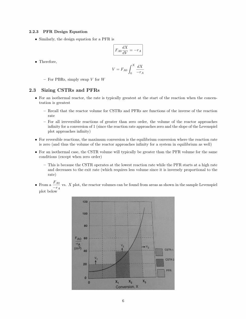
2.3 Sizing CSTRs and PFRs• For an isothermal reactor, the rate is typically greatest at the start of the reaction when the concen-

tration is greatest

– Recall that the reactor volume for CSTRs and PFRs are functions of the inverse of the reactionrate

– For all irreversible reactions of greater than zero order, the volume of the reactor approachesinfinity for a conversion of 1 (since the reaction rate approaches zero and the slope of the Levenspielplot approaches infinity)

• For reversible reactions, the maximum conversion is the equilibrium conversion where the reaction rateis zero (and thus the volume of the reactor approaches infinity for a system in equilibrium as well)

• For an isothermal case, the CSTR volume will typically be greater than the PFR volume for the sameconditions (except when zero order)

– This is because the CSTR operates at the lowest reaction rate while the PFR starts at a high rateand decreases to the exit rate (which requires less volume since it is inversely proportional to therate)

• From aFA0

−rAvs. X plot, the reactor volumes can be found from areas as shown in the sample Levenspiel

plot below

6

2.4 Reactors in Series• If we consider two CSTRs in series, we can state the following for the volume of one of the CSTRs

(where the f subscript stands for final and the i subscript stands for initial)

V = FA0

(1

−rA

)(Xf −Xi)

– If it is the first reactor in the series, then Xi = 0

• To achieve the same overall conversion, the total volume for two CSTRs in series is less than thatrequires for one CSTR (this is not true for PFRs)

• The volume for a PFR where PFRs are in series

V =

ˆ Xf

Xi

FA0dX

−rA

– PFRs in series have the same total volume for the same conversion as one PFR, as shown below:

Vtotal =

ˆ X2

0

FA0dX

−rA=

ˆ X1

0

FA0dX

−rA+

ˆ X2

X1

FA0dX

−rA

– A PFR can be modeled as infinitely many CSTRs in series

2.5 Space Time and Space Velocity• Space time is defined as

τ ≡ V

v0

– The velocity is measured at the entrance condition

– For a PBR,

τ ′ =W

v0= ρbτ

• Space velocity is defined asSV ≡ v0

V

– For a liquid-hourly space velocity (LHSV), the velocity is the liquid feed rate at 60 F or 75 F

– For a gas-hourly space velocity (GHSV), the velocity is measured at STP

3 Rate Laws and Stoichiometry

3.1 Rate Laws• The molecularity is the number of atoms, ions, or molecules colliding in a reaction step

• For a reaction aA+bB→cC+dD,−rAa

=−rBb

=rCc

=rDd

7

3.2 The Reaction Order and the Rate Law• A reaction rate is described as (using the reaction defined earlier),

−rA = kACαAC

βB

where the order with respect to A is α, the order with respect to B is β, and the total order is α+ β

• For a zero-order reaction, the units of k are mol/L·s

• For a first-order reaction, the units of k are 1/s

• For a second-order reaction, the units of k are L/mol·s

• For an elementary reaction, the rate law order is identical to the stoichiometric coefficients

• For heterogeneous reactions, partial pressures are used instead of concentrations

– To convert between partial pressure and concentration, one can use the ideal gas law– The reaction rate per unit volume is related to the rate of reaction per unit weight of catalyst via

−rA = ρ (−r′A)

• The equilibrium constant is defined (for the general reaction) as

KC =kforward

kreverse=CcC,eqC

dD,eq

CaA,eqCbB,eq

– The units of KC are (mol/L)d+c−b−a

• The net rate of formation of substance A is the sum of the rates of formation from the forward reactionand reverse reaction for a system at equilibrium

– For instance, if we have the elementary, reversible reaction of 2A B + C, we can state that−rA,forward = kAC

2A and rA,reverse = k−ACBCC . Therefore, −rA = − (rA,forward + rA,reverse) =

kAC2A − k−ACBCC = kA

(C2A −

k−AkA

CBCC

). Using KC =

CBCCC2A

, the previous expression can

be redefined as −rA = kA

(C2A −

CBCCKC

)• The temperature dependence of the concentration equilibrium constant is the following when there is

no change in the total number of moles and the heat capacity does not change

KC(T ) = KC(T1) exp

[∆H◦rxn

R

(1

T1− 1

T

)]3.3 The Reaction Rate Constant• The Arrhenius equation states that

kA(T ) = A exp

(− E

RT

)

• Plotting ln kA vs.1

Tyields a line with slope −E

Rand y-intercept is lnA

• Equivalently,

k(T ) = k(T0) exp

[E

R

(1

T0− 1

T

)]

8

3.4 Batch Systems• Let us define the following variables:

δ =d

a+c

a− b

a− 1

ΘB =NB0

NA0=CB0

CA0=yB0

yA0

• With these definitions, we can state that the total moles is described by

NT = NT0 + δNA0X

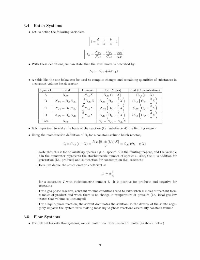
• A table like the one below can be used to compute changes and remaining quantities of substances ina constant volume batch reactor

Symbol Initial Change End (Moles) End (Concentration)A NA0 −NA0X NA0 (1−X) CA0 (1−X)

B NB0 = ΘBNA0 − baNA0X NA0

(ΘB −

b

aX

)CA0

(ΘB −

b

aX

)C NC0 = ΘCNA0

c

aNA0X NA0

(ΘC +

c

aX)

CA0

(ΘC +

c

aX)

D ND0 = ΘDNA0d

aNA0X NA0

(ΘD +

d

aX

)CA0

(ΘD +

d

aX

)Total NT0 NT = NT0 −NA0X

• It is important to make the basis of the reaction (i.e. substance A) the limiting reagent

• Using the mole-fraction definition of Θ, for a constant-volume batch reactor,

Ci = CA0 (1−X) =NA0 [Θi ± (i/a)X]

V= CA0 (Θi + νiX)

– Note that this is for an arbitrary species i 6= A, species A is the limiting reagent, and the variablei in the numerator represents the stoichiometric number of species i. Also, the ± is addition forgeneration (i.e. product) and subtraction for consumption (i.e. reactant)

– Here, we define the stoichiometric coefficient as

νI = ± ia

for a substance I with stoichiometric number i. It is positive for products and negative forreactants

– For a gas-phase reaction, constant-volume conditions tend to exist when n moles of reactant formn moles of product and when there is no change in temperature or pressure (i.e. ideal gas lawstates that volume is unchanged)

– For a liquid-phase reaction, the solvent dominates the solution, so the density of the solute negli-gibly impacts the system thus making most liquid-phase reactions essentially constant-volume

3.5 Flow Systems• For ICE tables with flow systems, we use molar flow rates instead of moles (as shown below)

9

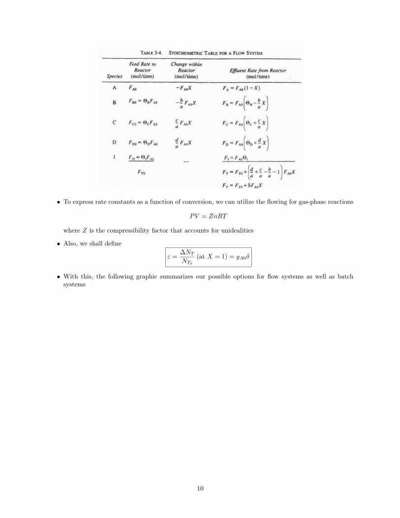
• To express rate constants as a function of conversion, we can utilize the flowing for gas-phase reactions

PV = ZnRT

where Z is the compressibility factor that accounts for unidealities

• Also, we shall define

ε =∆NTNT0

(at X = 1) = yA0δ

• With this, the following graphic summarizes our possible options for flow systems as well as batchsystems

10

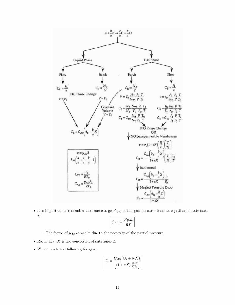
• It is important to remember that one can get CA0 in the gaseous state from an equation of state suchas

CA0 =PyA0

RT

– The factor of yA0 comes in due to the necessity of the partial pressure

• Recall that X is the conversion of substance A

• We can state the following for gases

Ci =CA0 (Θi + νiX)[(1 + εX) P0T

PT0

]

11

4 Isothermal Reactor Design

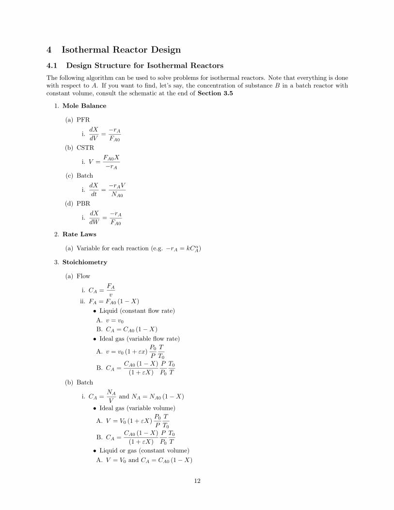
4.1 Design Structure for Isothermal ReactorsThe following algorithm can be used to solve problems for isothermal reactors. Note that everything is donewith respect to A. If you want to find, let’s say, the concentration of substance B in a batch reactor withconstant volume, consult the schematic at the end of Section 3.5

1. Mole Balance

(a) PFR

i.dX

dV=−rAFA0

(b) CSTR

i. V =FA0X

−rA(c) Batch

i.dX

dt=−rAVNA0

(d) PBR

i.dX

dW=−rAFA0

2. Rate Laws

(a) Variable for each reaction (e.g. −rA = kCαA)

3. Stoichiometry

(a) Flow

i. CA =FAv

ii. FA = FA0 (1−X)

• Liquid (constant flow rate)A. v = v0B. CA = CA0 (1−X)

• Ideal gas (variable flow rate)

A. v = v0 (1 + εx)P0

P

T

T0

B. CA =CA0 (1−X)

(1 + εX)

P

P0

T0T

(b) Batch

i. CA =NAV

and NA = NA0 (1−X)

• Ideal gas (variable volume)

A. V = V0 (1 + εX)P0

P

T

T0

B. CA =CA0 (1−X)

(1 + εX)

P

P0

T0T

• Liquid or gas (constant volume)A. V = V0 and CA = CA0 (1−X)

12

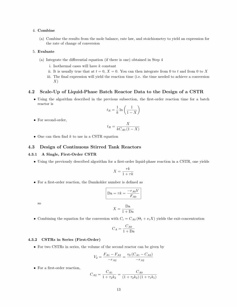
4. Combine

(a) Combine the results from the mole balance, rate law, and stoichiometry to yield an expression forthe rate of change of conversion

5. Evaluate

(a) Integrate the differential equation (if there is one) obtained in Step 4

i. Isothermal cases will have k constantii. It is usually true that at t = 0, X = 0. You can then integrate from 0 to t and from 0 to Xiii. The final expression will yield the reaction time (i.e. the time needed to achieve a conversion

X)

4.2 Scale-Up of Liquid-Phase Batch Reactor Data to the Design of a CSTR• Using the algorithm described in the previous subsection, the first-order reaction time for a batch

reactor istR =

1

kln

(1

1−X

)• For second-order,

tR =X

kCA0 (1−X)

• One can then find k to use in a CSTR equation

4.3 Design of Continuous Stirred Tank Reactors4.3.1 A Single, First-Order CSTR

• Using the previously described algorithm for a first-order liquid-phase reaction in a CSTR, one yields

X =τk

1 + τk

• For a first-order reaction, the Damkohler number is defined as

Da = τk =−rA0V

FA0

soX =

Da1 + Da

• Combining the equation for the conversion with Ci = CA0 (Θi + νiX) yields the exit-concentration

CA =CA0

1 + Da

4.3.2 CSTRs in Series (First-Order)

• For two CSTRs in series, the volume of the second reactor can be given by

V2 =FA1 − FA2

−rA2=v0 (CA1 − CA2)

−rA2

• For a first-order reaction,

CA2 =CA1

1 + τ2k2=

CA0

(1 + τ2k2) (1 + τ1k1)

13

• For a series of n CSTRs in series operating at the same temperature (constant k) and the same size(constant τ), the concentration leaving the final reactor is

CAn =CA0

(1 + τk)n =

CA0

(1 + Da)n

• Using CAn = CA0 (1−X),

X = 1− 1

(1 + Da)n

• The rate of disappearance of A for n CSTRs with first-order reactions is

−rAn = kCAn = kCA0

(1 + τk)n

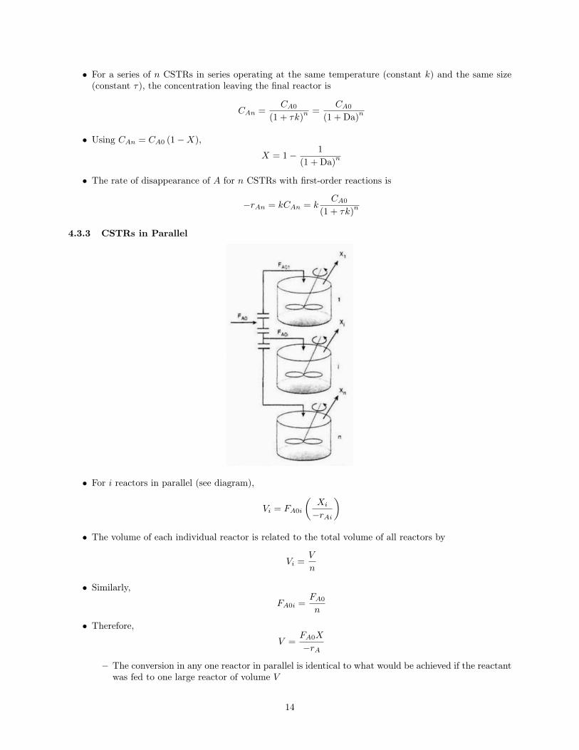
4.3.3 CSTRs in Parallel

• For i reactors in parallel (see diagram),

Vi = FA0i

(Xi

−rAi

)• The volume of each individual reactor is related to the total volume of all reactors by

Vi =V

n

• Similarly,

FA0i =FA0

n

• Therefore,

V =FA0X

−rA

– The conversion in any one reactor in parallel is identical to what would be achieved if the reactantwas fed to one large reactor of volume V

14

4.3.4 A Second-Order Reaction in a CSTR

• Using the algorithm discussed earlier in this section a second-order liquid-phase reaction in a CSTRhas

τ =CA0X

kC2A0 (1−X)

2

• When solved, this yields,

X =(1 + 2Da)−

√1 + 4Da

2Da

4.4 Tubular Reactors• Using the algorithm discussed earlier in this section, a second-order reaction in a PFR in the liquid-

phase yields

X =τkCA0

1 + τkCA0=

Da21 + Da2

whereDa2 = τkCA0

• For a second-order reaction in a PFR in the gas-phase at constant pressure and temperature2,

V =v0

kCA0

[2ε (1 + ε) ln (1−X) + ε2X +

(1 + ε)2X

1−X

]

– This equation states that when δ = 0, v = v0. When δ < 0, the volumetric flow rate decreases asthe conversion increases. When δ > 0, the volumetric flow increases as the conversion increases.This comes from the equation v = v0 (1 + εX) in this scenario

4.5 Pressure Drop in Reactors4.5.1 Ergun Equation

• The Ergun equation states that

dP

dz= − G

ρgcDp

(1− φφ3

)[150 (1− φ)µ

Dp+ 1.75G

]where φ is porosity (volume of void divided by total bed volume, or you can say that 1 − φ is thevolume of solid divided by total bed volume), gc is the gravitational constant, Dp is the diameter ofthe particle in the bed, µ is the viscosity of gas passing through the bed, z is the length down thepacked bed of pipe, ρ is the gas density, and G = ρu where u is the superficial velocity (volumetricflow divided by cross-sectional area of pipe)

4.5.2 PBR

• For a pressure drop through a packed bed,

dP

dz= −β0

P0TFTPT0FT0

where β0 is a constant composing the right hand side of the Ergun equation (without the negativesign)

2These expressions are quite specific for the reaction conditions but are easily derivable using the algorithm described at thebeginning of this section. Although the derivations are not shown in detail (see Fogler), you can check your work with theseresults. The general procedure does not vary.

15

• In terms of catalyst weightdP

dW=

−β0Ac (1− φ) ρc

P0TFTPT0FT0

• This can be expressed further asdy

dW= − α

2y

T

T0

FTFT0

where

α =2β0

Acρc (1− φ)P0

andy =

P

P0

– This equation should be used for membrane reactors or multiple reactors

• Some more manipulation yields the important equation,

dy

dW= − α

2y(1 + εX)

T

T0

– This equation should be coupled with

dX

dW= − rA

FA0

where you plug in the rate law and terms for the concentration

4.5.3 PFR

• For pressure drops in pipes (without packing) can be approximated by

P

P0= (1− αpV )

1/2

where

αp =4fG2

Acρ0P0D

and f is the fanning factor and u is the average velocity of the gas

4.6 Unsteady-State Operation of Stirred Reactors• The time to reach steady-state for an isothermal CSTR is given by

ts = 4.6τ

1 + τk

• For a semi-batch reactor, the volume as a function of time is

V = V0 + v0t

• The mole balance for a batch reactor is

dCAdt

= rA −v0VCA

• A mole balance on B for a batch reactor (if B is the fed substance) is

dCBdt

= rB +v0 (CB0 − CB)

V

16

4.7 Mole Balances on CSTRs, PFRs, PBRs, and Batch Reactors4.7.1 Liquid Phase

The mole balance for liquid-phase reactions of the type A+b

aB → c

aC +

d

aD is as follows:

1. Batch

(a)dCAdt

= rA

(b)dCBdt

=b

arA

2. CSTR

(a) V =v0 (CA0 − CA)

−rA

(b) V =v0 (CB0 − CB)

− (b/a) rA

3. PFR

(a) v0dCAdt

= rA

(b) v0dCBdV

=b

arA

4. PBR

(a) v0dCAdW

= rA

(b) v0dCBdW

=b

arA

4.7.2 Gas Phase

The mole balance for a gas-phase reaction is as follows:

FT =

n∑i=1

Fi

1. Batch

(a)dNidt

= riV

2. CSTR

(a) V =Fi0 − Fi−ri

3. PFR

(a)dFidV

= ri

The concentrations for a gas-phase reaction is as follows:

Ci = CT0FiT0FTT

y

17

5 Collection and Analysis of Rate Data

5.1 Batch Reactor Data5.1.1 Differential Method

• The following differential applies for constant-volume batch reactors,

ln

(−dCA

dt

)= α ln (CA) + ln (kA)

– Of course, this can be plotted as y = mx+ b to find the order, α

5.1.2 Integral Method

• In the integral method, we guess a reaction order and see if a plot gets a straight line

• For a zero-order reaction,CA = CA0 − kt

• For a first-order reaction,

ln

(CA0

CA

)= kt

• For a second-order reaction,1

CA= kt+

1

CA0

5.2 CSTR Reaction Data• Write down the stoichiometry equation relating CA and XA and solve for XA. For a gaseous system,

XA =1− CA/CA0

1 + εACA/2CA0

• Given v0 and CA, solve for XA. Then use the design equation of

−rA =v0CA0XA

V

to find the rate

• From here, plot ln (−rA) vs. ln (CA) to utilize

ln (−rA) = ln (k) + α ln (CA)

• If ε = 0, a plot of CA vs. τ will be linear for zeroth order with slope k

• If ε = 0, a plot ofCA0

CAvs. τ will be linear for first order with slope k

• If ε = 0, a plot ofCA0

CAvs. τCA will be linear for second order with slope k

18

5.3 PFR Reaction Data

• For any ε, a plot of XA vs.V

FA0can be made such that the tangent at any point has the value of −rA

• For zero order, a plot ofCA0 − CACA0 + εACA

vs.τ

CA0will have a slope of k

• For first order, a plot of (1 + εA) ln

(1

1−XA

)− εAXA vs. τ will have a slope of k

• For second order, a plot of 2εA (1 + εA) ln (1−XA) + ε2AXA + (εA + 1)2 XA

1−XAvs. τCA0 will have a

slope of k

5.4 Method of Initial Rates• Plot the logorithm of the initial rate (which can be obtained by the derivative at t = 0 of a series CA

vs. t plots) as a function of the logarithm of the initial concentration of A. The slope of the line is thereaction order with respect to A since −rA = kAC

αA

5.5 Method of Half-Lives• The equation for the half-life is

ln(t1/2

)= (1− α) ln (CA0) + ln

(2α−1 − 1

(α− 1) k

)– Therefore, by plotting ln

(t1/2

)against ln (CA0) , the order can be found as α = 1− slope

5.6 Differential Reactors• A series of experiments is carried out at different initial concentrations, and initial rate of reaction is

determined for each step

– The value of −rA0 can be found by differentiating the data and extrapolating to zero time

• The slope of ln (−rA0) vs. ln (CA0) will be α for a rate-law that follows a power-law with respect to A

• The design equations for the differential reactor are

−r′A =v0CA0 − CAexitv

∆W

and−r′A =

FA0X

∆W=Fproduct

∆W

19

6 Multiple Reactions

6.1 Definitions• The parallel reaction occurs when the reactant is consumed by two different reaction pathways to form

different prouncts (e.g. A breaks down to both B and C)

• The series reaction is when the reactant forms an intermediate product, which reacts further to formanother product (e.g.. A→ B → C)

• Complex reactions are multiple reactions that involve a combination of both series and parallel reactions

• Independent reactions occur are reactions that occur at the same time but neither the products norreactants react with themselves or one another (e.g. A→ B + C and D → E + F )

• The selectivity is defined as

S =rate of formation of desired product

rate of formation of undesired product

• The overall selectivity is defined as

S =exit molar flow rate of desired product

exit molar flow rate of undesired product

– For a CSTR, the overall selectivity and selectivity are identical

• The reaction yield is defined as the following if we A decomposes to a desired (D) and undesired (U)product

YD =rD−rA

• The overall yield for a batch system is

YD =ND

NA0 −NA

• The overall yield for a flow system is

YD =FD

FA0 − FA

– For a CSTR, the overall yield and instantaneous yield are identical

• For a CSTR, the highest overall yield (i.e. most product formed) occurs when the rectangle under theY vs. CA curve has the largest area

• For a PFR, the highest overall yield (i.e. most product formed) occurs when the area under the Y vs,CA curve is maximized

• If unreacted reagent can be separated from the exit stream and recycled, the highest overall yield (i.e.most product formed) is at the maximu of the Y vs. CA curve

20

6.2 Parallel Reactions6.2.1 Maximizing the Desired Product of One Reactant

Let α1 be the order of the desired reaction A + B → D and α2 be the order of the undesired reactionA + B → U . Let ED be the activation energy of the desired reaction and EU be the activation of theundesired reaction. We want to maximize selectivity.

• If α1 > α2:

– We want the concentration of the reactant to be as high as possible since Cα1−α2

A has a positiveexponent

– If in the gas phase, the reaction should be run without inerts and at high pressure

– If in the liquid phase, the reaction should be run without dilutents

– A batch or PFR should be used since CA starts at a high value and drops over the course of thereaction whereas it is always at the lowest concentration in a CSTR (i.e. the outlet concentration)

• If α2 > α1:

– We want the concentration of the reactant to be as low as possible since Cα1−α2

A has a negativeexponent

– If in the gas phase, the reaction should be run with inerts and at low pressure

– If in the liquid phase, the reaction should be run without dilutents

– A CSTR or recycle reactor should be used

• If ED > EU :

– High temperature should

• If EU > ED

– Low temperature should be used (but not so low that the desired reaction never proceeds)

• For analyzing the effect of activatoin energies on selectivity, one can state the following if the reactionis A→ D and A→ U

SD/U ∼kDkU

=ADAU

e−[(ED−EU )/(RT )]

– For a system of 3 reactions with a total of 2 undesired products, see Example 6-2 in Fogler forhow to analyze the temperature

6.2.2 Reactor Selection and Operating Conditions

Let α1 and β1 be the order of the desired reaction A + B → D and α2 and β2 be the order of the desiredreaction A + B → D if the reaction rates can be described by r = kCαAC

βB . We want to maximize the

selectivity of the desired product:

• If α1 > α2 and β1 > β2:

– Since Cα1−α2

A and Cβ1−β2

B both have poisitve exponents, the concentration of both A and B shouldbe maximized. Therefore, a tubular reactor or batch reactor should be used

– High pressure for a gas phase reaction and a minimization of inerts should be considered

• If α1 > α2 but β2 > β1:

21

– Since Cα1−α2

A has a positive exponent but Cβ1−β2

B has a negative exponent, the concentration ofA should be maximized, but the concentration of B should be minimized. Therfore, a semibatchreactor in which B is fed slowly into a large amount of A should be used.

– A membrane reactor or a tubular reactor with a side stream of B continuously fed into the reactorwould also work

– Another option is a series of small CSTRs with A fed only to the first reactor and small amountsof B fed to each reactor so thatB is mostly consumed before the CSTR exit stream flows into thenext reactor

• If α2 > α1 and β2 > β1:

– The concentration of both A and B should be minimized. Therefore, a CSTR should be used. Atubular reactor with a large recycle ratio can also be used

– The feed can be diluted with inerts and should be at low pressure if in the gas phase

• If α1 < α2 but β2 > β1:

– The concentration of A should be small but B should maximized. Therefore, a semibatch reactorwith A slowly fed to a large amount of B can be used

– A membrane reactor or a tubular reactor with side streams of A would also work– A series of small CSTRs with fres A fed to the reactor would be suitable as well

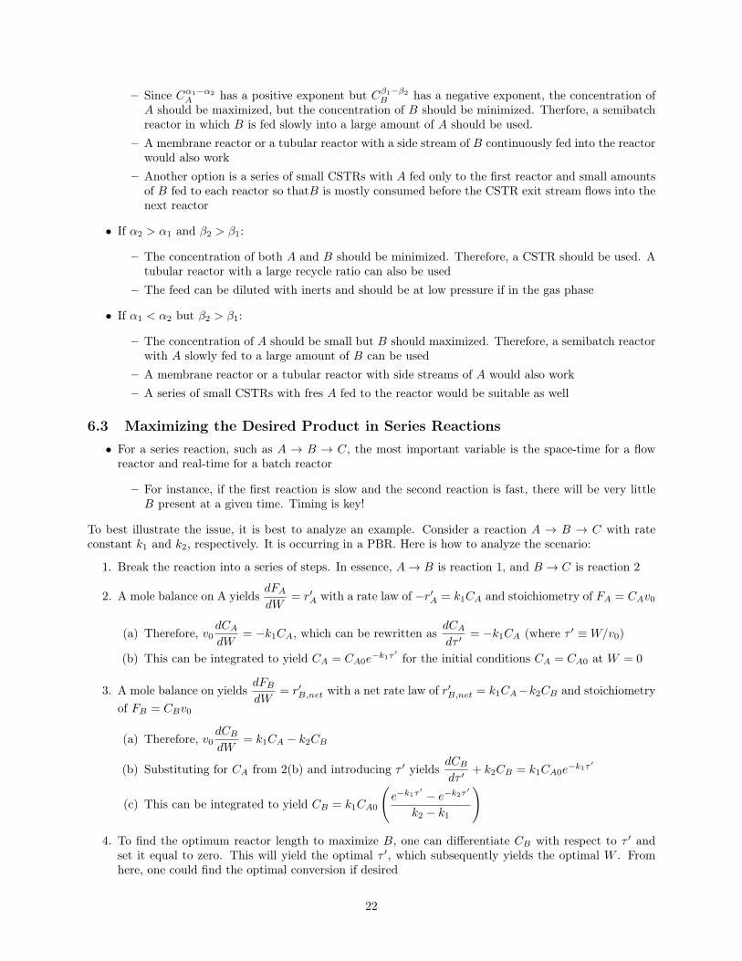
6.3 Maximizing the Desired Product in Series Reactions• For a series reaction, such as A → B → C, the most important variable is the space-time for a flow

reactor and real-time for a batch reactor

– For instance, if the first reaction is slow and the second reaction is fast, there will be very littleB present at a given time. Timing is key!

To best illustrate the issue, it is best to analyze an example. Consider a reaction A → B → C with rateconstant k1 and k2, respectively. It is occurring in a PBR. Here is how to analyze the scenario:

1. Break the reaction into a series of steps. In essence, A→ B is reaction 1, and B → C is reaction 2

2. A mole balance on A yieldsdFAdW

= r′A with a rate law of −r′A = k1CA and stoichiometry of FA = CAv0

(a) Therefore, v0dCAdW

= −k1CA, which can be rewritten asdCAdτ ′

= −k1CA (where τ ′ ≡W/v0)

(b) This can be integrated to yield CA = CA0e−k1τ ′ for the initial conditions CA = CA0 at W = 0

3. A mole balance on yieldsdFBdW

= r′B,net with a net rate law of r′B,net = k1CA−k2CB and stoichiometryof FB = CBv0

(a) Therefore, v0dCBdW

= k1CA − k2CB

(b) Substituting for CA from 2(b) and introducing τ ′ yieldsdCBdτ ′

+ k2CB = k1CA0e−k1τ ′

(c) This can be integrated to yield CB = k1CA0

(e−k1τ

′ − e−k2τ ′

k2 − k1

)

4. To find the optimum reactor length to maximize B, one can differentiate CB with respect to τ ′ andset it equal to zero. This will yield the optimal τ ′, which subsequently yields the optimal W . Fromhere, one could find the optimal conversion if desired

22

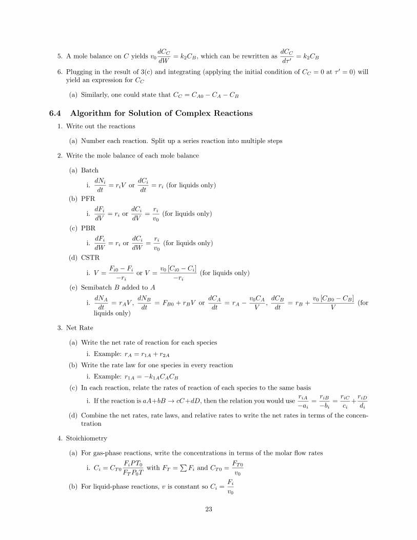
5. A mole balance on C yields v0dCCdW

= k2CB , which can be rewritten asdCCdτ ′

= k2CB

6. Plugging in the result of 3(c) and integrating (applying the initial condition of CC = 0 at τ ′ = 0) willyield an expression for CC

(a) Similarly, one could state that CC = CA0 − CA − CB

6.4 Algorithm for Solution of Complex Reactions1. Write out the reactions

(a) Number each reaction. Split up a series reaction into multiple steps

2. Write the mole balance of each mole balance

(a) Batch

i.dNidt

= riV ordCidt

= ri (for liquids only)

(b) PFR

i.dFidV

= ri ordCidV

=riv0

(for liquids only)

(c) PBR

i.dFidW

= ri ordCidW

=riv0

(for liquids only)

(d) CSTR

i. V =Fi0 − Fi−ri

or V =v0 [Ci0 − Ci]−ri

(for liquids only)

(e) Semibatch B added to A

i.dNAdt

= rAV ,dNBdt

= FB0 + rBV ordCAdt

= rA −v0CAV

,dCBdt

= rB +v0 [CB0 − CB ]

V(for

liquids only)

3. Net Rate

(a) Write the net rate of reaction for each species

i. Example: rA = r1A + r2A

(b) Write the rate law for one species in every reaction

i. Example: r1A = −k1ACACB(c) In each reaction, relate the rates of reaction of each species to the same basis

i. If the reaction is aA+bB → cC+dD, then the relation you would useriA−ai

=riB−bi

=riCci

+riDdi

(d) Combine the net rates, rate laws, and relative rates to write the net rates in terms of the concen-tration

4. Stoichiometry

(a) For gas-phase reactions, write the concentrations in terms of the molar flow rates

i. Ci = CT0FiPT0FTP0T

with FT =∑Fi and CT0 =

FT0

v0

(b) For liquid-phase reactions, v is constant so Ci =Fiv0

23

5. Pressure Drop

(a) Write the gas-phase pressure drop term in terms of molar flow rates

i.dy

dW= − α

2y

FTFT0

T

T0where y =

P

P0

6. Solve the system of ODEs

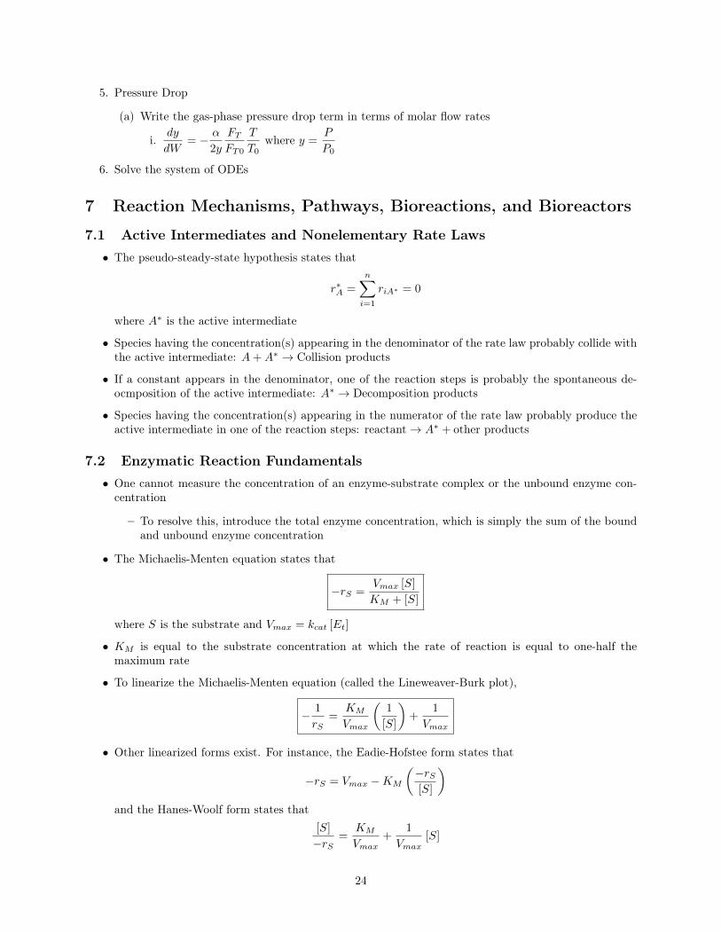
7 Reaction Mechanisms, Pathways, Bioreactions, and Bioreactors

7.1 Active Intermediates and Nonelementary Rate Laws• The pseudo-steady-state hypothesis states that

r∗A =

n∑i=1

riA∗ = 0

where A∗ is the active intermediate

• Species having the concentration(s) appearing in the denominator of the rate law probably collide withthe active intermediate: A+A∗ → Collision products

• If a constant appears in the denominator, one of the reaction steps is probably the spontaneous de-ocmposition of the active intermediate: A∗ → Decomposition products

• Species having the concentration(s) appearing in the numerator of the rate law probably produce theactive intermediate in one of the reaction steps: reactant→ A∗ + other products

7.2 Enzymatic Reaction Fundamentals• One cannot measure the concentration of an enzyme-substrate complex or the unbound enzyme con-

centration

– To resolve this, introduce the total enzyme concentration, which is simply the sum of the boundand unbound enzyme concentration

• The Michaelis-Menten equation states that

−rS =Vmax [S]

KM + [S]

where S is the substrate and Vmax = kcat [Et]

• KM is equal to the substrate concentration at which the rate of reaction is equal to one-half themaximum rate

• To linearize the Michaelis-Menten equation (called the Lineweaver-Burk plot),

− 1

rS=

KM

Vmax

(1

[S]

)+

1

Vmax

• Other linearized forms exist. For instance, the Eadie-Hofstee form states that

−rS = Vmax −KM

(−rS[S]

)and the Hanes-Woolf form states that

[S]

−rS=

KM

Vmax+

1

Vmax[S]

24

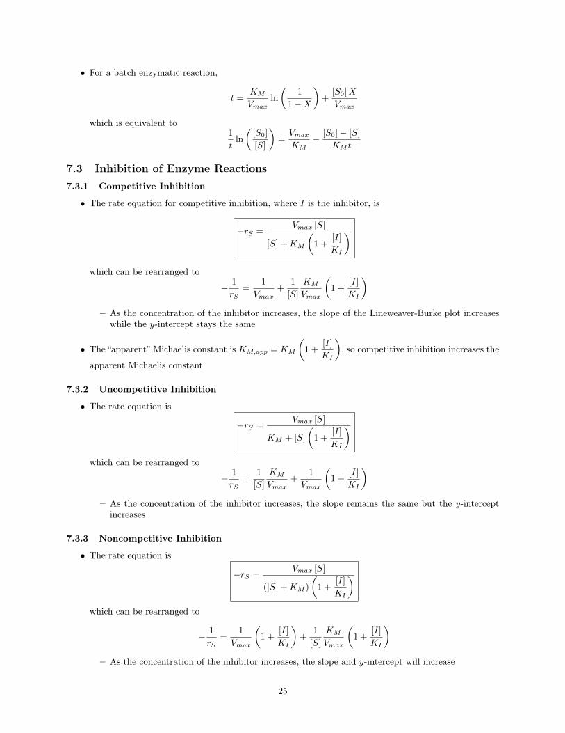
• For a batch enzymatic reaction,

t =KM

Vmaxln

(1

1−X

)+

[S0]X

Vmax

which is equivalent to1

tln

([S0]

[S]

)=VmaxKM

− [S0]− [S]

KM t

7.3 Inhibition of Enzyme Reactions7.3.1 Competitive Inhibition

• The rate equation for competitive inhibition, where I is the inhibitor, is

−rS =Vmax [S]

[S] +KM

(1 +

[I]

KI

)which can be rearranged to

− 1

rS=

1

Vmax+

1

[S]

KM

Vmax

(1 +

[I]

KI

)– As the concentration of the inhibitor increases, the slope of the Lineweaver-Burke plot increases

while the y-intercept stays the same

• The “apparent” Michaelis constant is KM,app = KM

(1 +

[I]

KI

), so competitive inhibition increases the

apparent Michaelis constant

7.3.2 Uncompetitive Inhibition

• The rate equation is

−rS =Vmax [S]

KM + [S]

(1 +

[I]

KI

)which can be rearranged to

− 1

rS=

1

[S]

KM

Vmax+

1

Vmax

(1 +

[I]

KI

)– As the concentration of the inhibitor increases, the slope remains the same but the y-intercept

increases

7.3.3 Noncompetitive Inhibition

• The rate equation is

−rS =Vmax [S]

([S] +KM )

(1 +

[I]

KI

)which can be rearranged to

− 1

rS=

1

Vmax

(1 +

[I]

KI

)+

1

[S]

KM

Vmax

(1 +

[I]

KI

)– As the concentration of the inhibitor increases, the slope and y-intercept will increase

25

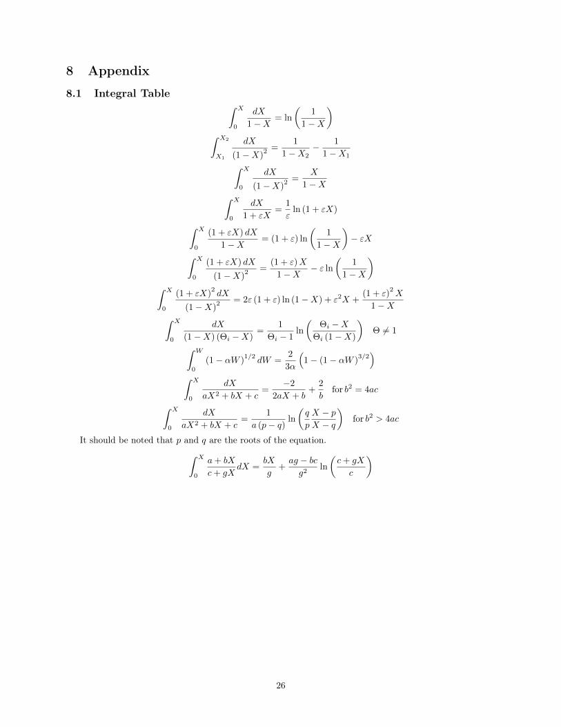
8 Appendix

8.1 Integral Tableˆ X

0

dX

1−X= ln

(1

1−X

)ˆ X2

X1

dX

(1−X)2 =

1

1−X2− 1

1−X1

ˆ X

0

dX

(1−X)2 =

X

1−Xˆ X

0

dX

1 + εX=

1

εln (1 + εX)

ˆ X

0

(1 + εX) dX

1−X= (1 + ε) ln

(1

1−X

)− εX

ˆ X

0

(1 + εX) dX

(1−X)2 =

(1 + ε)X

1−X− ε ln

(1

1−X

)ˆ X

0

(1 + εX)2dX

(1−X)2 = 2ε (1 + ε) ln (1−X) + ε2X +

(1 + ε)2X

1−Xˆ X

0

dX

(1−X) (Θi −X)=

1

Θi − 1ln

(Θi −X

Θi (1−X)

)Θ 6= 1

ˆ W

0

(1− αW )1/2

dW =2

3α

(1− (1− αW )

3/2)

ˆ X

0

dX

aX2 + bX + c=

−2

2aX + b+

2

bfor b2 = 4ac

ˆ X

0

dX

aX2 + bX + c=

1

a (p− q)ln

(q

p

X − pX − q

)for b2 > 4ac

It should be noted that p and q are the roots of the equation.ˆ X

0

a+ bX

c+ gXdX =

bX

g+ag − bcg2

ln

(c+ gX

c

)

26

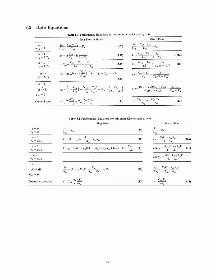
8.2 Rate Equations

27