Reactive point processes: A new approach to predicting ...web.mit.edu/rudin/www/docs/ErtekinRuMc15.pdf · 21,216 miles of underground cable, which is almost enough cable to wrap once

The Annals of Applied Statistics2015, Vol. 9, No. 1, 122–144DOI: 10.1214/14-AOAS789© Institute of Mathematical Statistics, 2015

REACTIVE POINT PROCESSES: A NEW APPROACH TOPREDICTING POWER FAILURES IN UNDERGROUND

ELECTRICAL SYSTEMS1

BY SEYDA ERTEKIN∗, CYNTHIA RUDIN∗ AND TYLER H. MCCORMICK†

Massachusetts Institute of Technology∗ and University of Washington†

Reactive point processes (RPPs) are a new statistical model designed forpredicting discrete events in time based on past history. RPPs were devel-oped to handle an important problem within the domain of electrical grid re-liability: short-term prediction of electrical grid failures (“manhole events”),including outages, fires, explosions and smoking manholes, which can causethreats to public safety and reliability of electrical service in cities. RPPs in-corporate self-exciting, self-regulating and saturating components. The self-excitement occurs as a result of a past event, which causes a temporaryrise in vulner ability to future events. The self-regulation occurs as a resultof an external inspection which temporarily lowers vulnerability to futureevents. RPPs can saturate when too many events or inspections occur closetogether, which ensures that the probability of an event stays within a realisticrange. Two of the operational challenges for power companies are (i) makingcontinuous-time failure predictions, and (ii) cost/benefit analysis for decisionmaking and proactive maintenance. RPPs are naturally suited for handlingboth of these challenges. We use the model to predict power-grid failures inManhattan over a short-term horizon, and to provide a cost/benefit analysisof different proactive maintenance programs.

1. Introduction. We present a new statistical model for predicting discreteevents over time, called Reactive Point Processes (RPPs). RPPs are a natural fitfor many different domains, and their development was motivated by the problemof predicting serious events (fires, explosions, power failures) in the undergroundelectrical grid of New York City (NYC). In New York City and in other majorurban centers, power-grid reliability is a major source of concern, as demand forelectrical power is expected to soon exceed the amount we are able to deliver withour current infrastructure [DOE (2008), NYBC (2010), Rhodes (2013)]. ManyAmerican electrical grids are massive and have been built gradually since the timeof Thomas Edison in the 1880s. For instance, in Manhattan alone, there are over21,216 miles of underground cable, which is almost enough cable to wrap oncearound the earth. Manhattan’s power distribution system is the oldest in the world,

Received July 2014; revised September 2014.1Supported in part by Con Edison, the MIT Energy Initiative Seed Fund and NSF CAREER Grant

IIS-1053407 to C. Rudin.Key words and phrases. Point processes, self-exciting processes, energy grid reliability, Bayesian

analysis, time-series.

122

http://www.imstat.org/aoas/

http://dx.doi.org/10.1214/14-AOAS789

http://www.imstat.org

REACTIVE POINT PROCESSES 123

and NYC’s power utility company, Con Edison, has cable databases that started inthe 1880s. Within the last decade, in order to handle increasing demands on NYC’spower-grid and increasing threats to public safety, Con Edison has developed anddeployed various proactive programs and policies [So (2004)]. In Manhattan, thereare approximately 53,000 access points to the underground electrical grid, whichare called electrical service structures or manholes. Problems in the undergrounddistribution network are manifested as problems within manholes, such as under-ground burnouts or serious events. A multi-year, ongoing collaboration to predictthese events in advance was started in 2007 [Rudin et al. (2010, 2012, 2014)],where diverse historical data were used to predict manhole events over a long-term horizon, as the data were not originally processed enough to predict events inthe short term. Being able to predict manhole events accurately in the short termcould immediately lead to reduced risks to public safety and increased reliabilityof electrical service. The data from this collaboration have sufficiently matureddue to iterations of the knowledge discovery process and maturation of the ConEdison inspections program, and, in this paper, we show that it is indeed possibleto predict manhole events to some extent within the short term.

The fact that RPPs are a generative model allows them to be used for cost-benefit analysis, and thus for policy decisions. In particular, since we can use RPPsto simulate power failures into the future, we can also simulate various inspectionpolicies that the power company might implement. This way we can create a robustsimulation setup for evaluating the relative costs of different inspection policiesfor NYC. This type of cost-benefit analysis can quantify the cost of the inspectionsprogram as it relates to the forecasted number of manhole events.

RPPs capture several important properties of power failures on the grid:

• There is an instantaneous rise in vulnerability to future serious events imme-diately following an occurrence of a past serious event, and the vulnerabilitygradually fades back to the baseline level. This is a type of self-exciting prop-erty.

• There is an instantaneous decrease in vulnerability due to an inspection, repairor other action taken. The effect of this inspection fades gradually over time.This is a self-regulating property.

• The cumulative effect of events or inspections can saturate, ensuring that vul-nerability levels never stray too far beyond their baseline level. This capturesdiminishing returns of many events or inspections in a row.

• The baseline level can be altered if there is at least one past event.• Vulnerability between similar entities should be similar. RPPs can be incorpo-

rated into a Bayesian framework that shares information across observably sim-ilar entities.

RPPs extend self-exciting point processes (SEPPs), which have only the self-exciting property mentioned above. Self-exciting processes date back at least tothe 1960s [Bartlett (1963), Kerstan (1964)]. The applicability of self-exciting

124 S. ERTEKIN, C. RUDIN AND T. H. MCCORMICK

point processes for modeling and analyzing time-series data has stimulated inter-est in diverse disciplines, including seismology [Ogata (1988, 1998)], criminology[Egesdal et al. (2010), Lewis et al. (2010), Louie, Masaki and Allenby (2010),Mohler et al. (2011), Porter and White (2012)], finance [Aït-Sahalia, Cacho-Diazand Laeven (2010), Bacry et al. (2013), Chehrazi and Weber (2011), Embrechts,Liniger and Lin (2011), Filimonov and Sornette (2012), Hardiman, Bercot andBouchaud (2013)], computational neuroscience [Johnson (1996), Krumin, Reutskyand Shoham (2010)], genome sequencing [Reynaud-Bouret and Schbath (2010)]and social networks [Crane and Sornette (2008), Du et al. (2013), Masuda et al.(2012), Mitchell and Cates (2010), Simma and Jordan (2010)]. These models ap-pear in so many different domains because they are a natural fit for time-seriesdata where one would like to predict discrete events in time, and where the oc-currence of a past event gives a temporary boost to the probability of an event inthe future. A recent work on Bayesian modeling for dependent point processesis that of Guttorp and Thorarinsdottir (2012). Paralleling the development of fre-quentist literature, many Bayesian approaches are motivated by data on naturalevents. Peruggia and Santner (1996), for example, develop a Bayesian frame-work for the Epidemic-Type-Aftershock-Sequences (ETAS) model. Nonparamet-ric Bayesian approaches for modeling data from nonhomogeneous point patterndata have also been developed [see Taddy and Kottas (2012), e.g.]. Blundell, Beckand Heller (2012) present a nonparametric Bayesian approach that uses Hawkesmodels for relational data. An expanded related work section appears in the sup-plementary material [Ertekin, Rudin and McCormick (2015)].

The self-regulating property can be thought of as the effect of an inspection.Inspections are made according to a predetermined policy of an external source,which may be deterministic or random. In the application that self-exciting pointprocesses are the most well known for, namely, earthquake modeling, it is not pos-sible to take an action to preemptively reduce the risk of an earthquake; however,in other applications it is clearly possible to do so. In our power failure applica-tion, power companies can perform preemptive inspections and repairs in orderto decrease electrical grid vulnerability. In neuroscience, it is possible to take anaction to temporarily reduce the firing rate of a neuron. There are many actionsthat police can take to temporarily reduce crime in an area (e.g., temporary in-creased patrolling or monitoring). In medical applications, doses of medicine canbe preemptively applied to reduce the probability of a cardiac arrest or other event.Alternatively, for instance, the self-regulation can come as a result of the patient’slab tests or visits to a physician.

Another way that RPPs expand upon SEPPs is that they allow deviations fromthe baseline vulnerability level to saturate. Even if there are repeated events orinspections in a short period of time, the vulnerability level still stays within arealistic range. In the original self-exciting point process model, it is possible forthe self-excitation to escalate to the point where the probability of an event getsvery close to one, which is generally unrealistic. In RPPs, the saturation function


prevents this from happening. Also, if many inspections are done in a row, thevulnerability level does not drop to zero, and there are diminishing returns for thelater ones because of the saturation function.

Outline of paper. We motivate RPPs using the power-grid application in Sec-tion 2. We first introduce the general form of the RPP model in Section 3. Wediscuss a Bayesian framework for fitting RPPs in Section 4. The Bayesian formu-lation, which we implement using Approximate Bayesian Computation (ABC),allows us to share information across observably similar entities (manholes in ourcase). For both methods we fit the model to NYC data and performed simulationstudies. Section 5 contains a prediction experiment, demonstrating the RPPs’ abil-ity to predict future events in NYC. Once the RPP model is fit to data from thepast, it can be used for simulation. In particular, we can simulate various inspec-tion policies for the Manhattan grid and examine the costs associated with eachof them in order to choose the best inspection policy. Section 6 shows this type ofsimulation using the RPP, illustrating how it is able to help choose between differ-ent inspection policies, and thus assist with broader policy decisions for the NYCinspections program. The paper’s supplementary material [Ertekin, Rudin and Mc-Cormick (2015)] includes a related work section, conditional frequency estimator(CF estimator) for the RPP, experiments with a maximum likelihood approach,a description of the inspection policy used in Section 6 and simulation studies forvalidating the fitting techniques for the models in the paper. It also includes a de-scription and link for a publicly available simulated data set that we generated,based on statistical properties of the Manhattan data set.

A short version of this paper appeared in the late-breaking developments trackof AAAI-13 [Ertekin, Rudin and McCormick (2013)].

2. Description of data. The data used for the project includes records fromthe Emergency Control Systems (ECS) trouble ticket system of Con Edison, whichincludes records of responses to past events (total 213,504 records for 53,525 man-holes from 1995 until 2010). Part of the trouble ticket for a manhole fire is inFigure 1.

Events can include serious problems such as manhole fires or explosions, ornonserious events such as wire burnouts. These tickets are heavily processed into astructured table, where each record indicates the time, manhole type (“service box”or “manhole,” and we refer to both types as manholes colloquially), the uniqueidentifier of the manhole and details about the event. The trouble tickets are clas-sified automatically as to whether they represent events (the kind we would liketo predict and prevent) or not (in which case the ticket is irrelevant and removed).The processing of tickets is based on a study where Con Edison engineers manu-ally labeled tickets, and is discussed further by Passonneau et al. (2011).


FDNY/250 REPORTS F/O 45536 E.51 ST & BEEKMAN PL...MANHOLE FIREMALDONADO REPORTS F/O 45536 E.51 ST FOUND SB-9960012 SMOKINGHEAVY...ACTIVE...SOLID...ROUND...NO STRAY VOLTAGE...29-L...SNOW...FLUSH REQUESTED...ORDERED #100103.12/22/09 08:10 MALDONADO REPORTS 3 2WAY-2WAY CRABS COPPEREDCUT OUT & REPLACED SAME. ALSO STATES 5 WIRE CROSSING COMES UP DEAD WILL INVESTIGATE IN SB-9960013.FLUSH # 100116 ORDERED FOR SAME12/22/09 14:00 REMARKS BELOW WERE ADDED BY 6235512/22/09 01:45 MASON REPORTS F/O 4553 E.51ST CLEARED ALLB/O-S IN SB9960013 ALSO FOUND A MAIN MISSING FROM THE WEST IN12/22/09 14:08 REMARKS BELOW WERE ADDED BY 62355SB9960011 F/O 1440 BEEKMAN................................JMC

FIG. 1. Part of the ECS remarks from a manhole fire ticket in 2009. The ticket implies that the man-hole was actively smoking upon the worker’s arrival. The worker located a crab connector that hadmelted (“coppered”) and a cable that was not carrying current (“dead”). Addresses and manholenumbers were changed for the purpose of anonymity.

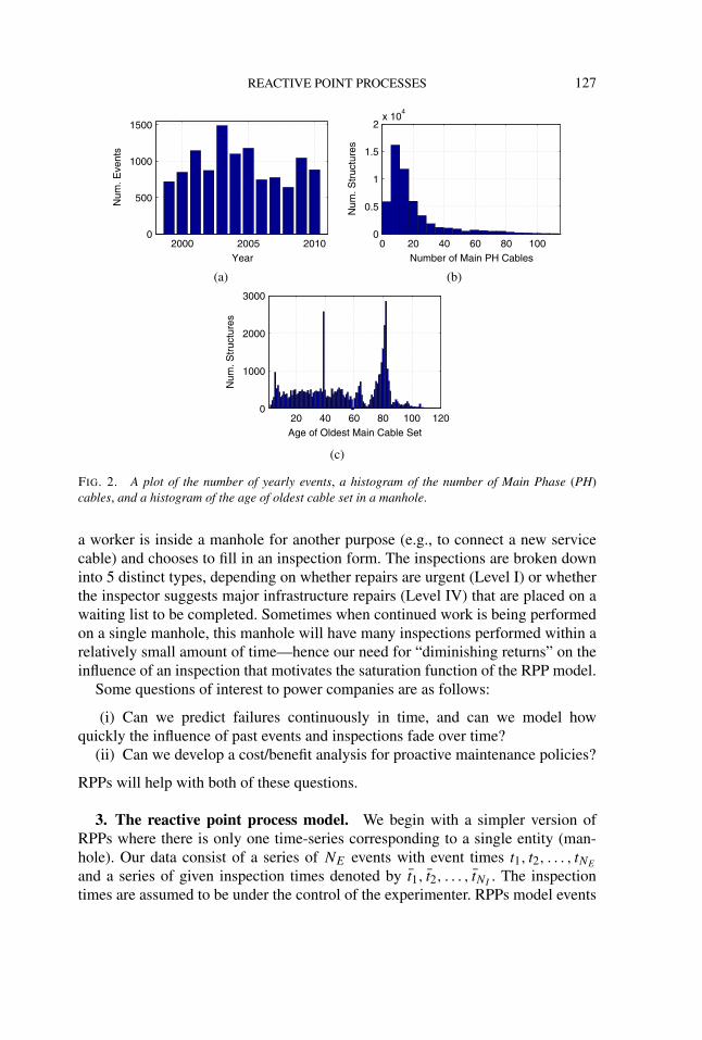
We have more or less complete event data from 1999 until the present, and in-complete event data between 1995 and 1999. A plot of the total number of eventsper year (using our definition of what constitutes an event) is provided in Fig-ure 2(a).

We also have manhole location and cable record information, which containsinformation about the underground electrical infrastructure. These two large tablesare joined together to determine which cables enter into which manholes. Theinferential join between the two tables required substantial processing in order tocorrectly match cables with manholes. Main cables are cables that connect twomanholes, as opposed to service or streetlight cables which connect to buildingsor streetlights. In our studies on long-term prediction of power failures, we havefound that the number of main phase cables in a manhole is a relatively usefulindicator of whether a manhole is likely to have an event. Figure 2(b) contains ahistogram of the number of main phase cables in a manhole.

The electrical grid was built gradually over the last ∼130 years, and, as a result,manholes often contain cables with a range of different ages. Figure 2(c) containsa histogram of the age of the oldest main cables in each manhole, as recorded inthe database. Cable age is also used as a feature for our RPP model. Cable agesrange from less than a year old to over 100 years old; Con Edison started keepingrecords back in the 1880s during the time of Thomas Edison. We remark that it isnot necessarily true that the oldest cables are the ones most in need of replacement.Many cables have been functioning for a century and are still functioning reliably.

We also have data from Con Edison’s new inspections program. Inspections canbe scheduled in advance, according to a schedule determined by a state mandate.This mandate currently requires an inspection for each structure at least once ev-ery 5 years. Con Edison also performs “ad hoc” inspections. These occur when


(a) (b)

(c)

FIG. 2. A plot of the number of yearly events, a histogram of the number of Main Phase (PH)cables, and a histogram of the age of oldest cable set in a manhole.

a worker is inside a manhole for another purpose (e.g., to connect a new servicecable) and chooses to fill in an inspection form. The inspections are broken downinto 5 distinct types, depending on whether repairs are urgent (Level I) or whetherthe inspector suggests major infrastructure repairs (Level IV) that are placed on awaiting list to be completed. Sometimes when continued work is being performedon a single manhole, this manhole will have many inspections performed within arelatively small amount of time—hence our need for “diminishing returns” on theinfluence of an inspection that motivates the saturation function of the RPP model.

Some questions of interest to power companies are as follows:

(i) Can we predict failures continuously in time, and can we model howquickly the influence of past events and inspections fade over time?

(ii) Can we develop a cost/benefit analysis for proactive maintenance policies?

RPPs will help with both of these questions.

3. The reactive point process model. We begin with a simpler version ofRPPs where there is only one time-series corresponding to a single entity (man-hole). Our data consist of a series of NE events with event times t1, t2, . . . , tNE

and a series of given inspection times denoted by t1, t2, . . . , tNI. The inspection

times are assumed to be under the control of the experimenter. RPPs model events


as being generated from a nonhomogeneous Poisson process with intensity λ(t)

where

λ(t) = λ0

[1 + g1

( ∑∀te<t

g2(t − te)

)− g3

( ∑∀ti<t

g4(t − ti )

)+ C11[NE≥1]

],(1)

where te are event times and ti are inspection times. The vulnerability level perma-nently goes up by C1 if there is at least one past event, where C1 is a constant thatcan be fitted. The C11[NE≥1] term is present to deal with “zero inflation,” where thecase of zero events needs to be handled separately than one or more past events.Functions g2 and g4 are the self-excitation and self-regulation functions, whichhave initially large amplitudes and decay over time. Self-exciting point processeshave only g2, and not the other functions, which are novel to RPPs. Functionsg1 and g3 are the saturation functions, which start out as the identity functionand then flatten farther from the origin. If the total sum of the excitation terms islarge, g1 will prevent the vulnerability level from increasing too much. Similarly,g4 controls the total possible amount of self-regulation and encodes “diminishingreturns” for having several inspections in a row.

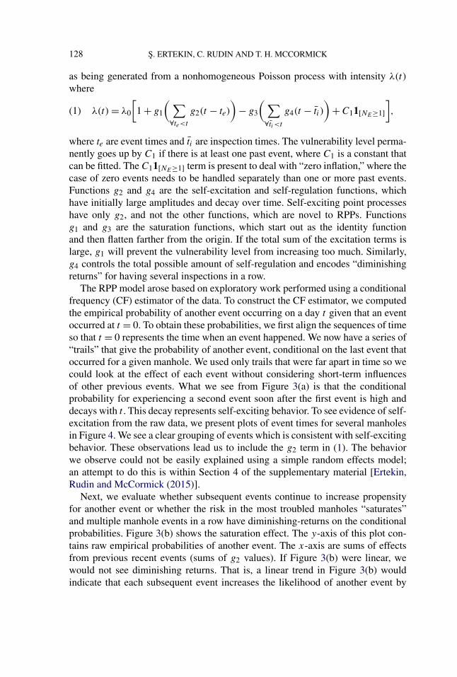
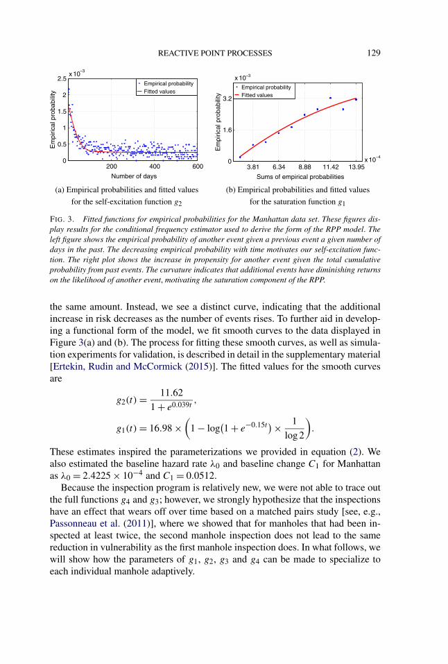
The RPP model arose based on exploratory work performed using a conditionalfrequency (CF) estimator of the data. To construct the CF estimator, we computedthe empirical probability of another event occurring on a day t given that an eventoccurred at t = 0. To obtain these probabilities, we first align the sequences of timeso that t = 0 represents the time when an event happened. We now have a series of“trails” that give the probability of another event, conditional on the last event thatoccurred for a given manhole. We used only trails that were far apart in time so wecould look at the effect of each event without considering short-term influencesof other previous events. What we see from Figure 3(a) is that the conditionalprobability for experiencing a second event soon after the first event is high anddecays with t . This decay represents self-exciting behavior. To see evidence of self-excitation from the raw data, we present plots of event times for several manholesin Figure 4. We see a clear grouping of events which is consistent with self-excitingbehavior. These observations lead us to include the g2 term in (1). The behaviorwe observe could not be easily explained using a simple random effects model;an attempt to do this is within Section 4 of the supplementary material [Ertekin,Rudin and McCormick (2015)].

Next, we evaluate whether subsequent events continue to increase propensityfor another event or whether the risk in the most troubled manholes “saturates”and multiple manhole events in a row have diminishing-returns on the conditionalprobabilities. Figure 3(b) shows the saturation effect. The y-axis of this plot con-tains raw empirical probabilities of another event. The x-axis are sums of effectsfrom previous recent events (sums of g2 values). If Figure 3(b) were linear, wewould not see diminishing returns. That is, a linear trend in Figure 3(b) wouldindicate that each subsequent event increases the likelihood of another event by


(a) Empirical probabilities and fitted values (b) Empirical probabilities and fitted values

for the self-excitation function g2 for the saturation function g1

FIG. 3. Fitted functions for empirical probabilities for the Manhattan data set. These figures dis-play results for the conditional frequency estimator used to derive the form of the RPP model. Theleft figure shows the empirical probability of another event given a previous event a given number ofdays in the past. The decreasing empirical probability with time motivates our self-excitation func-tion. The right plot shows the increase in propensity for another event given the total cumulativeprobability from past events. The curvature indicates that additional events have diminishing returnson the likelihood of another event, motivating the saturation component of the RPP.

the same amount. Instead, we see a distinct curve, indicating that the additionalincrease in risk decreases as the number of events rises. To further aid in develop-ing a functional form of the model, we fit smooth curves to the data displayed inFigure 3(a) and (b). The process for fitting these smooth curves, as well as simula-tion experiments for validation, is described in detail in the supplementary material[Ertekin, Rudin and McCormick (2015)]. The fitted values for the smooth curvesare

g2(t) = 11.62

1 + e0.039t,

g1(t) = 16.98 ×(

1 − log(1 + e−0.15t ) × 1

log 2

).

These estimates inspired the parameterizations we provided in equation (2). Wealso estimated the baseline hazard rate λ0 and baseline change C1 for Manhattanas λ0 = 2.4225 × 10−4 and C1 = 0.0512.

Because the inspection program is relatively new, we were not able to trace outthe full functions g4 and g3; however, we strongly hypothesize that the inspectionshave an effect that wears off over time based on a matched pairs study [see, e.g.,Passonneau et al. (2011)], where we showed that for manholes that had been in-spected at least twice, the second manhole inspection does not lead to the samereduction in vulnerability as the first manhole inspection does. In what follows, wewill show how the parameters of g1, g2, g3 and g4 can be made to specialize toeach individual manhole adaptively.


FIG. 4. Time of events in distinct manholes in the Manhattan data that demonstrate the self-exci-tating behavior. The x-axis is the number of days elapsed since the day of first record in the data setand the markers indicate the actual time of events.

Inspired by the CF estimator, we use the family of functions below for fittingpower-grid data, where a1, b1, a3, b3, β and γ are parameters that can be eithermodeled or fitted:

g1(ω) = a1 ×(

1 − 1

log 2log

(1 + e−b1ω

)), g2(t) = 1

1 + eβt,

(2)

g3(ω) = a3 ×(

1 − 1

log 2log

(1 + eb3ω

)), g4(t) = −1

1 + eγ t.

The factors of log 2 ensure that the vulnerability level is not negative.We need some notation in order to encode the possibility of multiple manholes.

In the case that there are multiple entities, there are P time-series, each corre-sponding to a unique entity p. For medical applications, each p is a patient, andfor the electrical grid reliability application, p is a manhole. Our data consist ofevents {t(p)e}p,e, inspections {t (p)i}p,i and, additionally, we may have covariateinformation Mp,j about every entity p, with covariates indexed by j . Covariatesfor the medical application might include a patient’s gender, age at the initial time,race, etc. For the manhole events application, covariates include the number ofmain phase cables in the manhole (number of current carrying cables between twomanholes), the total number of cable sets (total number of bundles of cables) in-cluding main, service and streetlight cables, and the age of the oldest cable setwithin the manhole. All covariates were normalized to be between −0.5 and 0.5.

Within the Bayesian framework, we can naturally incorporate the covariates tomodel functions λp for each p adaptively. Consider β in the expression for the self-excitation function g2 above. The β terms depend on individual-level covariates.In notation,

g(p)2 (t) = 1

1 + eβ(p)t, g

(p)4 (t) = −1

1 + eγ (p)t.(3)

The β(p)’s are assumed to be generated via a hierarchical model of the form

β = log(1 + e−Mυ)

where υ ∼ N(0, σ 2

υ

)


are the regression coefficients and M is the matrix of observed covariates. Theγ (p)’s are modeled hierarchically in the same manner,

γ = log(1 + e−Mω)

with ω ∼ N(0, σ 2

ω

).

This permits slower or faster decay of the self-exciting and self-regulating com-ponents based on the characteristics of the individual. For the electrical reliabilityapplication, we have noticed that manholes with more cables and older cables tendto have faster decay of the self-exciting terms, for instance.

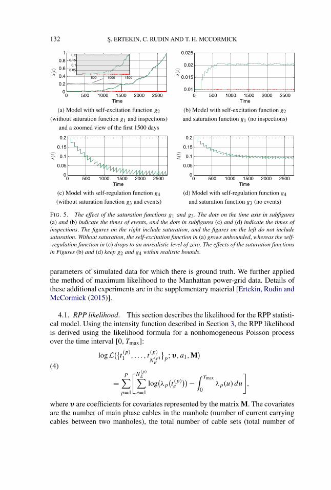
Demonstrating the need for the saturation function in the RPP model. In theprevious section we used exploratory tools on the Manhattan data to demonstratediminishing returns in risk for multiple subsequent events. In what follows, we linkthe exploratory work in the last section with our modeling framework, demonstrat-ing how the standard linear self-exciting process can produce unrealistic resultsunder ordinary conditions.

First we show that the self-excitation term can cause the rate of events λ(t) toincrease without bound. To show this, we considered a baseline vulnerability ofλ0 = 0.01, setting C1 = 0.1, used g2(t) = 1

1+e0.005t , and omitted the other compo-nents of the model (no inspections, no saturation g1). The self-excitation eventu-ally causes the rate of events to escalate unrealistically as shown in Figure 5 (upperleft). The embedded subfigure is a zoomed-in version of the first 1500 time steps.

When we include the saturation function g1, the excitation is controlled, andthe probability of an event no longer increases to unreasonable levels. We usedg1(ω) = 1 − 1

log 2 log(1 + e−ω), so that the vulnerability λ(t) can reach to a maxi-mum value of 0.021. The result is in Figure 5 (upper right).

Now we show the effect of the saturation function g3 in the presence of repeatedinspections. If no manhole events occur and the manhole is repeatedly inspected,then using the linear SEPP model, its vulnerability levels can become arbitrarilyclose to 0. This is not difficult to show, and we do this in Figure 5 (lower left). Herewe used λ0 = 0.2, g4(t) = −0.25

1+e0.002t , and omitted g3. We ran the same experiment

but with saturation, specifically, with g3(ω) = 1 − 1log 2 log(1 + eω). The results in

Figure 5 (lower right) show that the saturation function never lets the vulnerabilitydrop unrealistically far below the baseline level.

4. Fitting RPP statistical models. In this section we describe our Bayesianframework for inference using RPP models. The RPP intensity in equation (1)provides structure to capture self-excitation, self-regulation and saturation. First,in Section 4.1 we describe the likelihood for the RPP statistical model. We thendescribe prior distributions and our computational strategy for sampling from theposterior in Section 4.2. Section 4.3 then details the values we use in making pre-dictions. Along with the results presented here, we extensively evaluated our infer-ence strategy using a series of simulation experiments, where the goal is to recover


(a) Model with self-excitation function g2 (b) Model with self-excitation function g2

(without saturation function g1 and inspections) and saturation function g1 (no inspections)

and a zoomed view of the first 1500 days

(c) Model with self-regulation function g4 (d) Model with self-regulation function g4

(without saturation function g3 and events) and saturation function g3 (no events)

FIG. 5. The effect of the saturation functions g1 and g3. The dots on the time axis in subfigures(a) and (b) indicate the times of events, and the dots in subfigures (c) and (d) indicate the times ofinspections. The figures on the right include saturation, and the figures on the left do not includesaturation. Without saturation, the self-excitation function in (a) grows unbounded, whereas the self--regulation function in (c) drops to an unrealistic level of zero. The effects of the saturation functionsin Figures (b) and (d) keep g2 and g4 within realistic bounds.

parameters of simulated data for which there is ground truth. We further appliedthe method of maximum likelihood to the Manhattan power-grid data. Details ofthese additional experiments are in the supplementary material [Ertekin, Rudin andMcCormick (2015)].

4.1. RPP likelihood. This section describes the likelihood for the RPP statisti-cal model. Using the intensity function described in Section 3, the RPP likelihoodis derived using the likelihood formula for a nonhomogeneous Poisson processover the time interval [0, Tmax]:

logL({

t(p)1 , . . . , t

(p)

N(p)E

}p;υ, a1,M

)(4)

=P∑

p=1

[N(p)E∑

e=1

log(λp

(t (p)e

)) −∫ Tmax

0λp(u)du

],

where υ are coefficients for covariates represented by the matrix M. The covariatesare the number of main phase cables in the manhole (number of current carryingcables between two manholes), the total number of cable sets (total number of


bundles of cables) including main, service and streetlight cables, and the age of theoldest cable set within the manhole. All covariates were normalized to be between−0.5 and 0.5.

4.2. Bayesian RPP. Developing a Bayesian framework facilitates sharing ofinformation between observably similar manholes, thus making more efficient useof available covariate information. The RPP model encodes much of our prior in-formation into the shape of the rate function given in equation (1). As discussed inSection 3, we opted for a simple, parsimonious model that imposes mild regular-ization and information sharing without adding substantial additional information;specifically, we use diffuse Gaussian priors on the log scale for each regressioncoefficient.

We fit the model using Approximate Bayesian Computation [Diggle and Grat-ton (1984)]. The principle of Approximate Bayesian Computation (ABC) is torandomly choose proposed parameter values, use those values to generate data,and then compare the generated data to the observed data. If the difference is suf-ficiently small, then we accept the proposed parameters as draws from the ap-proximate posterior. To do ABC, we need two things: (i) to be able to simulatefrom the model and (ii) a summary statistic. To compare the generated and ob-served data, the summary statistic from the observed data, S({t (p)

1 , . . . , t(p)

N(p)E

}p),

is compared to that of the data simulated from the proposed parameter values,S({t (p),sim

1 , . . . , t(p),sim

N(p),simE

}p). If the values are similar, it indicates that the proposed

parameter values may yield a useful model for the data.A critical difference between updating a parameter value in an ABC iteration

versus, for example, a Metropolis–Hastings step is that ABC requires simulatingfrom the likelihood, whereas Metropolis–Hastings requires evaluating the likeli-hood. In our context, we are able to both evaluate and simulate from the likelihoodwith approximately the same computational complexity. ABC has some advan-tages, namely, that we have meaningful summary statistics, discussed below. Fur-ther, in our case it is not particularly computationally challenging, as we alreadyextensively simulate from the model as a means of evaluating hypothetical inspec-tion policies. We evaluated the adequacy of this method extensively in simulationstudies presented in the supplementary material [Ertekin, Rudin and McCormick(2015)].

A key conceptual aspect of ABC is that one can choose the summary statistic tobest match the problem. The sufficient statistic for the RPP is the vector of eventtimes, and thus gives no data reduction—so we choose other statistics. One impor-tant insight in constructing our summary statistic is that changing the parametersin the RPP model alters the distribution of times between events. The histogram oftime differences for a homogenous Poisson Process, for example, has an exponen-tial decay. The self-exciting process, on the other hand, has a distribution resem-bling a lognormal because of the positive association between intensities after an


event occurs. Altering the parameters of the RPP model changes the intensity ofself-excitation and self-regulation, thus altering the distribution of times betweenevents. We construct our first statistic, therefore, by examining the KL divergencebetween the distribution of times between events in the data and the distributionbetween event times in the simulated data. We do this for each of our proposed pa-rameters. Examining the distribution of times between events, though not the truesufficient statistic, captures a concise and low-dimensional summary of a key fea-ture of the process. This statistic does not, however, capture the overall prevalenceof events in the process. Since we focus only on the distribution of times betweenevents, various processes with different overall intensity could produce distribu-tions with similar KL divergence to the data distribution. We therefore introducea second statistic that counts the total number of events. We contend that togetherthese statistics represent both the spacing and the overall scale (or frequency) ofevents. Thus, the two summary measures we use are as follows:

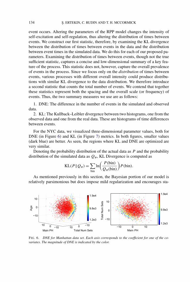
1. DNE: The difference in the number of events in the simulated and observeddata.

2. KL: The Kullback–Leibler divergence between two histograms, one from theobserved data and one from the real data. These are histograms of time differencesbetween events.

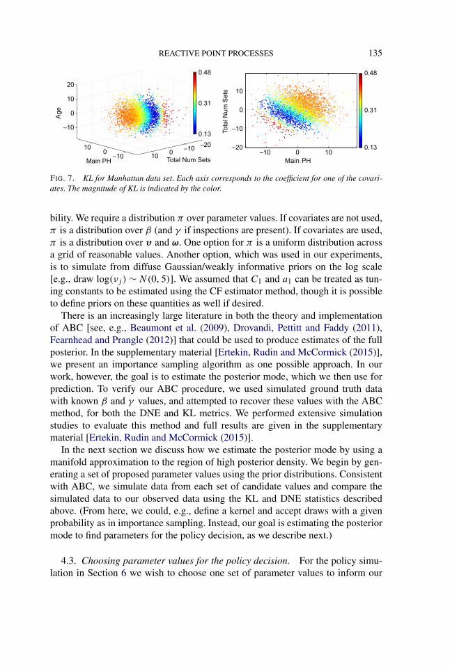
For the NYC data, we visualized three-dimensional parameter values, both forDNE (in Figure 6) and KL (in Figure 7) metrics. In both figures, smaller values(dark blue) are better. As seen, the regions where KL and DNE are optimized arevery similar.

Denoting the probability distribution of the actual data as P and the probabilitydistribution of the simulated data as Qυ , KL Divergence is computed as

KL(P‖Qυ) = ∑bin

ln(

P(bin)

Qυ(bin)

)P(bin).

As mentioned previously in this section, the Bayesian portion of our model isrelatively parsimonious but does impose mild regularization and encourages sta-

FIG. 6. DNE for Manhattan data set. Each axis corresponds to the coefficient for one of the co-variates. The magnitude of DNE is indicated by the color.


FIG. 7. KL for Manhattan data set. Each axis corresponds to the coefficient for one of the covari-ates. The magnitude of KL is indicated by the color.

bility. We require a distribution π over parameter values. If covariates are not used,π is a distribution over β (and γ if inspections are present). If covariates are used,π is a distribution over υ and ω. One option for π is a uniform distribution acrossa grid of reasonable values. Another option, which was used in our experiments,is to simulate from diffuse Gaussian/weakly informative priors on the log scale[e.g., draw log(νj ) ∼ N(0,5)]. We assumed that C1 and a1 can be treated as tun-ing constants to be estimated using the CF estimator method, though it is possibleto define priors on these quantities as well if desired.

There is an increasingly large literature in both the theory and implementationof ABC [see, e.g., Beaumont et al. (2009), Drovandi, Pettitt and Faddy (2011),Fearnhead and Prangle (2012)] that could be used to produce estimates of the fullposterior. In the supplementary material [Ertekin, Rudin and McCormick (2015)],we present an importance sampling algorithm as one possible approach. In ourwork, however, the goal is to estimate the posterior mode, which we then use forprediction. To verify our ABC procedure, we used simulated ground truth datawith known β and γ values, and attempted to recover these values with the ABCmethod, for both the DNE and KL metrics. We performed extensive simulationstudies to evaluate this method and full results are given in the supplementarymaterial [Ertekin, Rudin and McCormick (2015)].

In the next section we discuss how we estimate the posterior mode by using amanifold approximation to the region of high posterior density. We begin by gen-erating a set of proposed parameter values using the prior distributions. Consistentwith ABC, we simulate data from each set of candidate values and compare thesimulated data to our observed data using the KL and DNE statistics describedabove. (From here, we could, e.g., define a kernel and accept draws with a givenprobability as in importance sampling. Instead, our goal is estimating the posteriormode to find parameters for the policy decision, as we describe next.)

4.3. Choosing parameter values for the policy decision. For the policy simu-lation in Section 6 we wish to choose one set of parameter values to inform our


FIG. 8. Fitted manifold of υ values with smallest KL divergence and smallest DNE.

decision. In order to choose a single best value of the parameters, we fit a polyno-mial manifold to the intersection of the bottom 10% of KL values and the bottom10% of DNE values. Defining υ1, υ2 and υ3 as the coefficients for number of mainphase cables, age of oldest main cable set and total number of sets features, theformula for the manifold is

υ3 = −9.6 − 0.98υ1 − 0.13υ2 − 1.1 × 10−3(υ1)2 − 3.6 × 10−3υ1υ2

+ 4.67 × 10−2(υ2)2,

which is determined by a least squares fit to the data. The fitted manifold is shownin Figure 8 along with the data.

We then optimized for the point on the manifold closest to the origin. Thisimplicitly adds regularization, as it chooses the parameter values closest to theorigin. This point is υ1 = −4.6554, υ2 = −0.5716, and υ3 = −4.8028.

Note that cable age (corresponding to the second coefficient) is not the mostimportant feature defining the manifold. As previous studies have shown [Rudinet al. (2010)], even though there are very old cables in the city, the age of cableswithin a manhole is not alone the best predictor of vulnerability. Now we alsoknow that it is not the best predictor of the rate of decay of vulnerability back tobaseline levels. This supports Con Edison’s goal to prioritize the most vulnerablecomponents of the power-grid, rather than simply replacing the oldest components.The features that mainly determine decay of the self-excitation function g2 are thenumber of main phase cables and the number of cable sets. As either or both ofthese numbers increase, decay rate β increases, meaning that manholes with morecables tend to return to baseline levels faster than manholes with fewer cables.

5. Predicting events on the NYC power-grid. Our first experiment aims toevaluate whether the CF estimator or the feature-based strategy introduced aboveis better in terms of identifying the most vulnerable manholes. To do this, we se-lected 5000 manholes (rank 1001–6000 from the project’s current long-term pre-diction model). These manholes have similar vulnerability levels, which allows usto isolate the self-exciting effect without modeling the baseline level. Using both


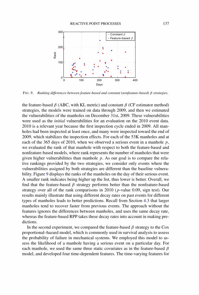
FIG. 9. Ranking differences between feature-based and constant (nonfeature-based) β strategies.

the feature-based β (ABC, with KL metric) and constant β (CF estimator method)strategies, the models were trained on data through 2009, and then we estimatedthe vulnerabilities of the manholes on December 31st, 2009. These vulnerabilitieswere used as the initial vulnerabilities for an evaluation on the 2010 event data.2010 is a relevant year because the first inspection cycle ended in 2009. All man-holes had been inspected at least once, and many were inspected toward the end of2009, which stabilizes the inspection effects. For each of the 53K manholes and ateach of the 365 days of 2010, when we observed a serious event in a manhole p,we evaluated the rank of that manhole with respect to both the feature-based andnonfeature-based models, where rank represents the number of manholes that weregiven higher vulnerabilities than manhole p. As our goal is to compare the rela-tive rankings provided by the two strategies, we consider only events where thevulnerabilities assigned by both strategies are different than the baseline vulnera-bility. Figure 9 displays the ranks of the manholes on the day of their serious event.A smaller rank indicates being higher up the list, thus lower is better. Overall, wefind that the feature-based β strategy performs better than the nonfeature-basedstrategy over all of the rank comparisons in 2010 (p-value 0.09, sign test). Ourresults mainly illustrate that using different decay rates on past events for differenttypes of manholes leads to better predictions. Recall from Section 4.3 that largermanholes tend to recover faster from previous events. The approach without thefeatures ignores the differences between manholes, and uses the same decay rate,whereas the feature-based RPP takes these decay rates into account in making pre-dictions.

In the second experiment, we compared the feature-based β strategy to the Coxproportional–hazard model, which is commonly used in survival analysis to assessthe probability of failure in mechanical systems. We employed this model to as-sess the likelihood of a manhole having a serious event on a particular day. Foreach manhole, we used the same three static covariates as in the feature-based β

model, and developed four time-dependent features. The time-varying features for


day t are (1) the number of times the manhole was a trouble hole (source of theproblem) for a serious event until t , (2) the number of times the manhole was atrouble hole for a serious event in the last year, (3) the number of times the man-hole was a trouble hole for a precursor event (less serious event) until t , and (4)the number of times the manhole was a trouble hole for a precursor event in thelast year. The feature-based β model currently does not differentiate serious andprecursor events, though it is a direct extension to do this if desired. The modelwas trained using the coxph function in the R survival package using data priorto 2009, and then predictions were made on the test set of 5000 manholes in the2010 data set. These predictions were transformed into ranked lists of manholesfor each day. We then compared the ranks achieved by the Cox model with theranks of manholes at the time of events. The difference of aggregate ranks was infavor of the feature-based β approach (p-value 7e–06, sign test), indicating that thefeature-based β strategy provides a substantial advantage in its ability to prioritizevulnerable manholes.

The Cox model we compared with represents a “long-term” model similar towhat we were using previously for manhole event prediction on Con Edison data[Rudin et al. (2010)]. The Cox model considers different information, namely,counts of past events. These counts are time-varying, but the past events do notsmoothly wear off in time as they do for the RPP. The fact that the RPP model iscompetitive with the Cox model indicates that the effects of past manhole eventsdo wear off with time (in agreement with Figure 3 where we traced the decaydirectly using data). The saturating elements of the model ensure that the modelis physically plausible, since we showed in Section 3 that the results could beunphysical (with rates going to 0 or above 1) without the saturation.

6. Making broader policy decisions using RPPs. Because the RPP modelis a generative model, it can be used to simulate the future, and thus assist withbroader policy decisions regarding how often inspections should be performed.This can be used to justify allocation of spending. Con Edison’s existing inspectionpolicy is a combination of targeted periodic inspections and ad hoc inspections.The targeted inspections are planned in advance, whereas the ad hoc inspectionsare unscheduled. An ad hoc inspection could be performed while a utility worker isin the process of, for instance, installing a new service cable to a building or repair-ing an outage. Either source of inspection can result in an urgent repair (Type I), animportant but not urgent repair (Type II), a suggested structural repair (Types IIIand IV), or no repair, or any combination of repairs. Urgent repairs need to becompleted before the inspector leaves the manhole, whereas Type IV repairs areplaced on a waiting list. According to the current inspections policy, each manholeundergoes a targeted inspection every 5 years. The choice of inspection policy tosimulate can be determined very flexibly, and any inspection policy and hypothe-sized effect of inspections can be examined through simulation.


As a demonstration, we conducted a simulation over a 20 year future time hori-zon that permits a cost-benefit analysis of the inspection program, when targetedinspections are performed at a given frequency. To do this simulation, we requirethe following:

• A characterization of manhole vulnerability. For Manhattan, this is learned fromthe past using the ABC RPP feature-based β training strategy for the saturationfunction g1 and the self-excitation function g2 discussed above. Saturation andself-regulation functions g3 and g4 for the inspection program cannot yet belearned due to the newness of the inspection program and are discussed below.

• An inspection policy. The policy can include targeted, ad hoc or history-basedinspections. We chose to evaluate “bright line” inspection policies, where eachmanhole is inspected once in each Y year period, where Y is varied (discussedbelow). We also included an ad hoc inspection policy that visits 3 manholes perday on average.

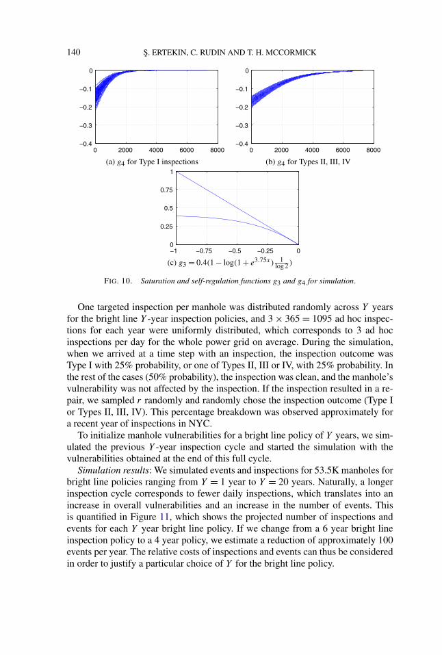
Effect of inspections: The effect of inspections on the overall vulnerability ofmanholes were designed in consultation with domain experts. The choices aresomewhat conservative, so as to give a lower bound for costs. The effect of anurgent repair (Type I) is different from the effect of less urgent repairs (Types II,III and IV). For all inspection types, after 1 year beyond the time of the inspec-tion, the effect of the inspection decays to, on average, 85% of its initial effect, inagreement with a short-term empirical study on inspections. (There is some un-certainty in this initial effect, and the initial drop in vulnerability is chosen froma normal distribution so that after one year the effect decays to a mean of 85%.)For Type I inspections, the effect of the inspection decays to baseline levels afterapproximately 3000 days, and for Types II, III and IV, which are more extensiverepairs, the effect fully decays after 7000 days. In particular, we use the followingg4 functions:

gType I4 (t) = −83.7989 × (

r × 5 × 10−4 + 3.5 × 10−3) × 1

1 + e0.0018t,(5)

gTypes II,III,IV4 (t) = −49.014 × (

r × 5 × 10−4 + 7 × 10−3) × 1

1 + e0.00068t,(6)

where r is randomly sampled from a standard normal distribution. For all inspec-tion types, we used the following g3 saturation function:

g3(t) = 0.4 ×(

1 − log(1 + e−3.75t ) × 1

log 2

),

which ensures that subsequent inspections do not lower the vulnerability to morethan 60% of the baseline vulnerability. Sampled g4 functions for Type I andTypes II, II, IV, along with g3 are shown in Figure 10.


(a) g4 for Type I inspections (b) g4 for Types II, III, IV

(c) g3 = 0.4(1 − log(1 + e3.75x) 1log 2 )

FIG. 10. Saturation and self-regulation functions g3 and g4 for simulation.

One targeted inspection per manhole was distributed randomly across Y yearsfor the bright line Y -year inspection policies, and 3 × 365 = 1095 ad hoc inspec-tions for each year were uniformly distributed, which corresponds to 3 ad hocinspections per day for the whole power grid on average. During the simulation,when we arrived at a time step with an inspection, the inspection outcome wasType I with 25% probability, or one of Types II, III or IV, with 25% probability. Inthe rest of the cases (50% probability), the inspection was clean, and the manhole’svulnerability was not affected by the inspection. If the inspection resulted in a re-pair, we sampled r randomly and randomly chose the inspection outcome (Type Ior Types II, III, IV). This percentage breakdown was observed approximately fora recent year of inspections in NYC.

To initialize manhole vulnerabilities for a bright line policy of Y years, we sim-ulated the previous Y -year inspection cycle and started the simulation with thevulnerabilities obtained at the end of this full cycle.

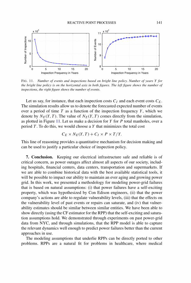
Simulation results: We simulated events and inspections for 53.5K manholes forbright line policies ranging from Y = 1 year to Y = 20 years. Naturally, a longerinspection cycle corresponds to fewer daily inspections, which translates into anincrease in overall vulnerabilities and an increase in the number of events. Thisis quantified in Figure 11, which shows the projected number of inspections andevents for each Y year bright line policy. If we change from a 6 year bright lineinspection policy to a 4 year policy, we estimate a reduction of approximately 100events per year. The relative costs of inspections and events can thus be consideredin order to justify a particular choice of Y for the bright line policy.


FIG. 11. Number of events and inspections based on bright line policy. Number of years Y forthe bright line policy is on the horizontal axis in both figures. The left figure shows the number ofinspections, the right figure shows the number of events.

Let us say, for instance, that each inspection costs CI and each event costs CE .The simulation results allow us to denote the forecasted expected number of eventsover a period of time T as a function of the inspection frequency Y , which wedenote by NE(Y,T ). The value of NE(Y,T ) comes directly from the simulation,as plotted in Figure 11. Let us make a decision for Y for P total manholes, over aperiod T . To do this, we would choose a Y that minimizes the total cost

CE × NE(Y,T ) + CI × P × T/Y.

This line of reasoning provides a quantitative mechanism for decision making andcan be used to justify a particular choice of inspection policy.

7. Conclusion. Keeping our electrical infrastructure safe and reliable is ofcritical concern, as power outages affect almost all aspects of our society, includ-ing hospitals, financial centers, data centers, transportation and supermarkets. Ifwe are able to combine historical data with the best available statistical tools, itwill be possible to impact our ability to maintain an ever aging and growing powergrid. In this work, we presented a methodology for modeling power-grid failuresthat is based on natural assumptions: (i) that power failures have a self-excitingproperty, which was hypothesized by Con Edison engineers, (ii) that the powercompany’s actions are able to regulate vulnerability levels, (iii) that the effects onthe vulnerability level of past events or repairs can saturate, and (iv) that vulner-ability estimates should be similar between similar entities. We have been able toshow directly (using the CF estimator for the RPP) that the self-exciting and satura-tion assumptions hold. We demonstrated through experiments on past power-griddata from NYC, and through simulations, that the RPP model is able to capturethe relevant dynamics well enough to predict power failures better than the currentapproaches in use.

The modeling assumptions that underlie RPPs can be directly ported to otherproblems. RPPs are a natural fit for problems in healthcare, where medical


conditions cause self-excitation and treatments provide regulation. Through theBayesian framework we introduced, RPPs extend to a broad range of problemswhere predictive power can be pooled among multiple related entities, whethermanholes or medical patients.

The results presented in this work show for the first time that manhole eventscan be predicted in the short term, which was previously thought not to be possi-ble. Knowing how one might do this permits us to take preventive action to keepvulnerability levels low, and can help make broader policy decisions for power-grid maintenance through simulation of many uncertain futures, simulated overany desired policy.

SUPPLEMENTARY MATERIAL

Supplementary material for “Reactive point processes: A new approach topredicting power failures in underground electrical systems” (DOI: 10.1214/14-AOAS789SUPP; .pdf). The supplementary material includes an expanded re-lated work section, conditional frequency estimator (CF estimator) for the RPP,experiments with a maximum likelihood approach, a description of the inspec-tion policy used in Section 6, an analysis of Manhattan data using random effectsmodel and simulation studies for validating the fitting techniques for the models inthe paper. It also includes a description and link for a publicly available simulateddata set that we generated, based on statistical properties of the Manhattan dataset.

REFERENCES

AÏT-SAHALIA, Y., CACHO-DIAZ, J. and LAEVEN, R. J. (2010). Modeling financial contagion us-ing mutually exciting jump processes. Technical report, National Bureau of Economic Research,Cambridge, MA.

BACRY, E., DELATTRE, S., HOFFMANN, M. and MUZY, J. F. (2013). Modelling microstructurenoise with mutually exciting point processes. Quant. Finance 13 65–77. MR3005350

BARTLETT, M. S. (1963). The spectral analysis of point processes. J. R. Stat. Soc. Ser. B Stat.Methodol. 25 264–296. MR0171334

BEAUMONT, M. A., CORNUET, J.-M., MARIN, J.-M. and ROBERT, C. P. (2009). Adaptive ap-proximate Bayesian computation. Biometrika 96 983–990. MR2767283

BLUNDELL, C., BECK, J. and HELLER, K. A. (2012). Modelling reciprocating relationships withHawkes processes. In Advances in Neural Information Processing Systems 25. Curran Associates,Red Hook, NY.

CHEHRAZI, N. and WEBER, T. A. (2011). Dynamic valuation of delinquent credit-card accounts.Working paper.

CRANE, R. and SORNETTE, D. (2008). Robust dynamic classes revealed by measuring the responsefunction of a social system. Proc. Natl. Acad. Sci. USA 105 15649–15653.

DIGGLE, P. J. and GRATTON, R. J. (1984). Monte Carlo methods of inference for implicit statisticalmodels. J. R. Stat. Soc. Ser. B Stat. Methodol. 46 193–227. MR0781880

DOE (2008). The Smart Grid, An Introduction. Technical report. Prepared by Litos Strategic Com-munication. US Dept. Energy, Office of Electricity Delivery & Energy Reliability.

http://dx.doi.org/10.1214/14-AOAS789SUPP

http://www.ams.org/mathscinet-getitem?mr=3005350






DROVANDI, C. C., PETTITT, A. N. and FADDY, M. J. (2011). Approximate Bayesian computationusing indirect inference. J. R. Stat. Soc. Ser. C. Appl. Stat. 60 317–337. MR2767849

DU, N., SONG, L., WOO, H. and ZHA, H. (2013). Uncover topic-sensitive information diffusionnetworks. In Proceedings of the Sixteenth International Conference on Artificial Intelligence andStatistics 229–237.

EGESDAL, M., FATHAUER, C., LOUIE, K., NEUMAN, J., MOHLER, G. and LEWIS, E. (2010). Sta-tistical and stochastic modeling of gang rivalries in Los Angeles. SIAM Undergraduate ResearchOnline 3 72–94.

EMBRECHTS, P., LINIGER, T. and LIN, L. (2011). Multivariate Hawkes processes: An applicationto financial data. J. Appl. Probab. 48A 367–378. MR2865638

ERTEKIN, S., RUDIN, C. and MCCORMICK, T. (2013). Predicting Power Failures with ReactivePoint Processes. In AAAI Workshop on Late-Breaking Developments. AAAI Press, Menlo Park,CA.

ERTEKIN, S., RUDIN, C. and MCCORMICK, T. H. (2015). Supplement to “Reactive point processes:A new approach to predicting power failures in underground electrical systems.” DOI:10.1214/14-AOAS789SUPP.

FEARNHEAD, P. and PRANGLE, D. (2012). Constructing summary statistics for approximateBayesian computation: Semi-automatic approximate Bayesian computation. J. R. Stat. Soc. Ser. BStat. Methodol. 74 419–474. MR2925370

FILIMONOV, V. and SORNETTE, D. (2012). Quantifying reflexivity in financial markets: Toward aprediction of flash crashes. Phys. Rev. E (3) 85 056108.

GUTTORP, P. and THORARINSDOTTIR, T. L. (2012). Bayesian inference for non-Markovian pointprocesses. In Advances and Challenges in Space–Time Modeling of Natural Events (E. Porcu,J.-M. Montero and M. Schlather, eds.) 79–102. Springer, Berlin.

HARDIMAN, S. J., BERCOT, N. and BOUCHAUD, J.-P. (2013). Critical reflexivity in financial mar-kets: A Hawkes process analysis. Eur. Phys. J. B 86 1–9.

JOHNSON, D. H. (1996). Point process models of single-neuron discharges. J. Comput. Neurosci. 3275–299.

KERSTAN, J. (1964). Teilprozesse Poissonscher Prozesse. In Trans. Third Prague Conf. InformationTheory, Statist. Decision Functions, Random Processes (Liblice, 1962) 377–403. Publ. HouseCzech. Acad. Sci., Prague. MR0166826

KRUMIN, M., REUTSKY, I. and SHOHAM, S. (2010). Correlation-based analysis and generation ofmultiple spike trains using hawkes models with an exogenous input. Front. Comput. Neurosci. 4147.

LEWIS, E., MOHLER, G., BRANTINGHAM, P. J. and BERTOZZI, A. (2010). Self-exciting pointprocess models of insurgency in Iraq. UCLA CAM Reports 10-38.

LOUIE, K., MASAKI, M. and ALLENBY, M. (2010). A point process model for simulating gang-on-gang violence. Technical report, UCLA.

MASUDA, N., TAKAGUCHI, T., SATO, N. and YANO, K. (2012). Self-exciting point process mod-eling of conversation event sequences. Preprint. Available at arXiv:1205.5109.

MITCHELL, L. and CATES, M. E. (2010). Hawkes process as a model of social interactions: A viewon video dynamics. J. Phys. A 43 045101, 11. MR2578723

MOHLER, G. O., SHORT, M. B., BRANTINGHAM, P. J., SCHOENBERG, F. P. and TITA, G. E.(2011). Self-exciting point process modeling of crime. J. Amer. Statist. Assoc. 106 100–108.MR2816705

NYBC (2010). Electricity OUTLOOK: Powering New York City’s economic future. Technical re-port. New York Building Congress Reports: Energy Outlook 2010–2025.

OGATA, Y. (1988). Statistical models for earthquake occurrences and residual analysis for pointprocesses. J. Amer. Statist. Assoc. 83 9–27.

OGATA, Y. (1998). Space–time point-process models for earthquake occurrences. Ann. Inst. Statist.Math. 50 379–402.






http://arxiv.org/abs/arXiv:1205.5109





PASSONNEAU, R., RUDIN, C., RADEVA, A., TOMAR, A. and XIE, B. (2011). Treatment effect ofrepairs to an electrical grid: Leveraging a machine learned model of structure vulnerability. InProceedings of the KDD Workshop on Data Mining Applications in Sustainability (SustKDD),17th Annual ACM SIGKDD Conference on Knowledge Discovery and Data Mining. ACM, NewYork.

PERUGGIA, M. and SANTNER, T. (1996). Bayesian analysis of time evolution of earthquakes.J. Amer. Statist. Assoc. 91 1209–1218.

PORTER, M. D. and WHITE, G. (2012). Self-exciting hurdle models for terrorist activity. Ann. Appl.Stat. 6 106–124. MR2951531

REYNAUD-BOURET, P. and SCHBATH, S. (2010). Adaptive estimation for Hawkes processes; ap-plication to genome analysis. Ann. Statist. 38 2781–2822. MR2722456

RHODES, L. (2013). US power grid has issues with reliability. Data Center Knowledge(www.datacenterknowledge.com): Industry Perspectives.

RUDIN, C., PASSONNEAU, R. J., RADEVA, A., DUTTA, H., IEROME, S. and ISAAC, D. (2010).A process for predicting manhole events in Manhattan. Mach. Learn. 80 1–31. MR3108158

RUDIN, C., WALTZ, D., ANDERSON, R. N., BOULANGER, A., SALLEB-AOUISSI, A., CHOW, M.,DUTTA, H., GROSS, P. N., HUANG, B., IEROME, S., ISAAC, D. F., KRESSNER, A., PASSON-NEAU, R. J., RADEVA, A. and WU, L. (2012). Machine learning for the New York City powergrid. IEEE Trans. Pattern. Anal. Mach. Intell. 34 328–345.

RUDIN, C., ERTEKIN, S., PASSONNEAU, R., RADEVA, A., TOMAR, A., XIE, B., LEWIS, S., RID-DLE, M., PANGSRIVINIJ, D. and MCCORMICK, T. (2014). Analytics for power grid distributionreliability in New York City. Interfaces 44 364–383.

SIMMA, A. and JORDAN, M. I. (2010). Modeling Events with Cascades of Poisson Processes. InProc. of the 26th Conference on Uncertainty in Artificial Intelligence (UAI2010). AUAI Press.

SO, H. (2004). Council approves bill on Con Ed annual inspections. The Villager 74 23.TADDY, M. A. and KOTTAS, A. (2012). Mixture modeling for marked Poisson processes. Bayesian

Anal. 7 335–361. MR2934954

S. ERTEKIN

C. RUDIN

MIT COMPUTER SCIENCE

AND ARTIFICIAL INTELLIGENCE LABORATORY

AND

MIT SLOAN SCHOOL OF MANAGEMENT

MASSACHUSETTS INSTITUTE OF TECHNOLOGY

CAMBRIDGE, MASSACHUSETTS 02139USAE-MAIL: [email protected]

[email protected]

T. H. MCCORMICK

DEPARTMENT OF STATISTICS

UNIVERSITY OF WASHINGTON

SEATTLE, WASHINGTON 98195USAE-MAIL: [email protected]



http://www.datacenterknowledge.com



mailto:[email protected]



Documents

Reactive point processes: A new approach to predicting ...web.mit.edu/rudin/www/docs/ErtekinRuMc15.pdf · 21,216 miles of underground cable, which is almost enough cable to wrap once