Embed Size (px)
Citation preview
Research Division Federal Reserve Bank of St. Louis Working Paper Series
Reaction Functions in a Small Open Economy:
What Role for Non-traded Inflation?
Ana Maria Santacreu
Working Paper 2014-044A
http://research.stlouisfed.org/wp/2014/2014-044.pdf
November 2014
FEDERAL RESERVE BANK OF ST. LOUIS
Research Division P.O. Box 442
St. Louis, MO 63166
______________________________________________________________________________________
The views expressed are those of the individual authors and do not necessarily reflect official positions of the Federal Reserve Bank of St. Louis, the Federal Reserve System, or the Board of Governors.
Federal Reserve Bank of St. Louis Working Papers are preliminary materials circulated to stimulate discussion and critical comment. References in publications to Federal Reserve Bank of St. Louis Working Papers (other than an acknowledgment that the writer has had access to unpublished material) should be cleared with the author or authors.
Reaction functions in a small open economy:
What role for non-traded in�ation?∗
Ana Maria Santacreu†
June 2005
Abstract
I develop a structural general equilibrium model and estimate it for
New Zealand using Bayesian techniques. The estimated model considers
a monetary policy regime where the central bank targets overall in�a-
tion but is also concerned about output, exchange rate movements, and
interest rate smoothing. Taking the posterior mean of the estimated pa-
rameters as representing the characteristics of the New Zealand economy,
I compare the consequences that two alternative reaction functions have
on the central bank's loss, for di�erent speci�cations of its preferences. I
obtain conditions under which the monetary authority should respond di-
rectly to non-tradable in�ation instead of overall in�ation. In particular,
if preferences are relatively biased towards in�ation stabilization, respond-
ing directly to overall in�ation results in better macroeconomic outcomes.
If instead the central bank places relatively more weight on output stabi-
lization, responding directly to non-traded in�ation is a better strategy.
JEL Classi�cation: C51, E52, F41
Key Words: monetary policy, non-traded in�ation, reaction functions,
small open economy
∗This paper was prepared while visiting the Reserve Bank of New Zealand. The author
thanks Aaron Drew, Kirdan Lees, Thomas Lubik, Christie Smith, Shaun Vahey and John
Williams for useful comments, and the Reserve Bank of New Zealand for its hospitality during
the visit.†INSEAD
1
1
1 Introduction
In this paper I apply Bayesian techniques to estimate a model of asmall open economy with traded and non-traded sectors. Althoughthere are a number of papers that explore this kind of setting, noconsensus has yet been reached about the type of monetary policy thatshould be followed in a multisectoral economy. I examine this issue byestablishing whether the central bank’s reaction function should bedriven by overall inflation (headline inflation in the consumer priceindex) or by a measure of ‘domestic’ inflation.
My analysis focuses on the New Zealand (NZ) economy. As the firsteconomy to introduce inflation targeting, the available data sample islonger than for any of the economies that subsequently adopted thistype of monetary policy regime. This fact makes it appealing to studythe New Zealand economy.
Adopting a multisectoral perspective is likely to be important for NewZealand for a number of reasons. New Zealand is a commodity-focusedeconomy and thus produces different products to those it consumes.In small open economies a significant proportion of total consumptioncomes from imports. Because New Zealand is small and geographi-cally isolated, there exists a large non-tradables sector. Historically,the aggregate and non-tradable sectors have had differing levels of pricechange (refer to figures 3 and 3 in appendix A).1 Although CPI inflationremained inside the Reserve Bank of New Zealand’s target range dur-ing 2004 and the first half of 2005, non-tradable inflation was above 4percent during the same period. Non-tradable inflation has been offsetin the CPI by relatively low tradable inflation, reflecting the appreci-ation of the exchange rate.2 These features mean that developing amultisectoral model is likely to be particularly valuable.
A major area of research activity in recent years is the so called ‘new
1This characteristic has been noted not only in New Zealand, but also in other economies likeAustralia and Canada, Bharucha and Kent (1998) and Ortega and Rebei (2005).
2For further details see RBNZ (2005).
2
open economy macroeconomics’.3 I develop a model within that frame-work and estimate it for the New Zealand economy using the Bayesianmethodology developed by Schorfheide (2000). This type of modelhas been applied to countries like the United States (US) and the Eu-ropean Union. In this paper, however, the focus is on a small andvery open economy with features different than those found in large,almost-closed economies.
According to the 2002 Policy Target Agreements, the Reserve Bankof New Zealand’s (RBNZ) primary price stability objective is aug-mented with secondary considerations for output variability, exchangerate movements, and interest rate smoothing. This suggests the impor-tance of considering the industrial structure of the economy – the splitbetween tradable and non-tradable sectors – when targeting inflation.4
In contrast to other authors that have analyzed monetary policy inthe framework of ‘new open macroeconomic models’, I consider thedistinction between traded and non-traded goods, similar to Lubik(2003). There are both empirical and theoretical reasons for the centralbank of a small open economy to consider the industrial structure ofthe economy. Empirically, traded and non-traded inflation appear tohave different stochastic characteristics. From an empirical point ofview, the data suggest that the variability of the economic variablesat the disaggregate level is higher than at the aggregate level. As wecan see in tables 4 and 5, this is the case for small open economies likeNew Zealand, Canada, and Australia.
One reason for these sectoral differences is that the two sectors areinfluenced by monetary policy in different ways. The traded sector isaffected by both the exchange rate and interest rate channels of mone-tary policy, while the non-traded sector is only exposed to the latter. If
3See Obstfeld and Rogoff (2000).4The Reserve Bank of New Zealand Act 1989 specifies that the primary function of the Reserve
Bank shall be to deliver ‘stability in the general level of prices.’ Section 9 of the Act then saysthat the Minister of Finance and the Governor of the Reserve Bank shall together have a separateagreement setting out specific targets for achieving and maintaining price stability. This is known asthe Policy Targets Agreement (PTA). For more information, visit www.rbnz.govt.nz/monpol/pta.
3
the central bank does not take into account the different transmissionmechanisms, and instead simply aggregates both sectors, it could mis-step in setting policy. Furthermore, since different sectors are drivenby different shock processes, a separate treatment of the sectors im-proves the central bank’s understanding of the inflation process andtherefore its ability to meet its inflation targeting objective.
The rest of the paper is as follows. The theoretical model is presentedin section 2. It builds on the model by Gali and Monacelli (2005),but differentiates between traded and non-traded sectors. In section3, I estimate the model following the Bayesian methodology developedby Schorfheide (2000) and used in Lubik and Schorfheide (2005). Aprocedure to test if the model fits the data, based on the comparisonbetween the empirical and the model cross-covariances, is also brieflydiscussed. Section 4 presents the analysis of alternative monetary pol-icy reaction functions: in one case the central bank responds directlyto overall inflation, and in the other the central bank responds directlyto non-traded inflation. Section 4 identifies conditions under whichresponding directly to non-traded-inflation is the best alternative. Fi-nally, section 5 concludes.
2 The model
I consider a small open economy that is characterized by the existenceof two domestic sectors: a home traded goods sector and a non-tradedgoods sector.5 In both sectors prices are sticky according to a Calvo-staggered setting, modified to allow some backward-looking behaviourby firms.6 Each sector is subject to a specific productivity shock.
I assume complete financial markets: households have access to a com-plete set of contingent claims that are traded in international markets.
5 According to the RBNZ definition, the tradable goods sector comprises all those goods andservices that are imported or that are in competition with foreign goods, either in domestic or foreignmarkets. The non-tradable sector comprises all those goods that do not face foreign competition.
6I consider a hybrid Phillips curve in the same sense as Gali and Gertler (1999).
4
This eliminates one potential source of distortion. The only distortionsin the economy are due to sticky prices and firms’ monopoly power.
The model is closed with alternative Taylor-type policy rules where thecentral bank responds not only to inflation but also to output growth,interest rates and changes in the nominal exchange rate. This allowsme to model and compare different monetary regimes.
There are seven structural shocks in this economy: two productivityshocks, corresponding to each domestic sector, a government shock, amonetary policy shock, and three shocks related to the foreign econ-omy. Apart from these shocks I consider two measurement errors thatcorrespond to deviations from uncovered interest parity (UIP) andterms of trade.
2.1 The consumer’s problem
There is a representative household which maximizes the intertemporalutility function
E0
∞∑t=0
βt
(C1−σ
t
1 − σ− N 1+ψ
t
1 + ψ
)(1)
subject to the intertemporal budget constraint. σ is the inverse of theelasticity of substitution between consumption and labour and ψ is theinverse labour elasticity. In equation (1)
Ct = Ct − hCt−1 (2)
where h is the parameter of habit persistence, which is an importantfeature of the model. Recent empirical analysis of aggregate data hasobtained substantial evidence of habit persistence.7 Ct is a consump-tion index consisting of differentiated goods and Nt is total labour
7The idea of habit formation dates back to Duesenberry (1949). Deaton and Muellbauer (1980)provide a survey and early references. These preferences have been used in a rich variety of contexts.Some applications in the real business cycle literature include Boldrin, Christiano and Fisher (2001),Fuhrer (2000), and Lettau and Uhlig (2000).
5
effort. Labour is supplied to both traded and non-traded sector in thefollowing way,
Nt = NH,t + NN,t (3)
where the subscript H refers to ‘home-produced’ tradables, and thesubscript N refers to the non-tradable sector. Labour is completelymobile across sectors, which implies that wages in the traded and non-traded sectors are identical.
In aggregate, and assuming complete asset markets, the household’sbudget constraint is
PtCt + Et(Qt+1Dt+1) ≤ Dt + WtNt + Tt (4)
Pt is the price index, Dt+1 is the nominal payoff in period t + 1 of theportfolio held at the end of period t, Qt,t+1 is the stochastic discountfactor, Wt is the nominal wage, and Tt are lump-sum taxes.8
The consumption bundle, Ct is a constant elasticity of substitution(CES) index composed of both tradable, CT,t and non-tradable goods,CN,t,
Ct =((1 − λ)1/νC
ν−1ν
T,t + λ1/νCν−1
ν
N,t
) νν−1
(5)
where λ is the share of non-tradable goods in the economy and ν isthe intratemporal elasticity of substitution between tradable and non-tradable goods at Home. I assume ν > 0.
Households allocate aggregate expenditure based on the following de-mand functions:
CT,t = (1 − λ)
(PT,t
Pt
)−ν
Ct (6)
CN,t = λ
(PN,t
Pt
)−ν
Ct (7)
8Note that money is not modelled in the utility function or in the budget constraint. I assumea cashless economy where the coefficient of the real money balances in the utility function can beapproximated to zero.
6
Tradable goods consumption is determined as a CES index composedof the tradable goods that home consumers buy from the home sectorand the goods bought from the foreign sector,
CT,t =
((1 − α)1/ηC
η−1η
H,t + α1/ηCη−1
η
F,t
) ηη−1
(8)
where α is the share of the foreign consumption component in thetradable consumption index and η is the intratemporal elasticity ofsubstitution between home and foreign goods.
The demand for domestic goods and imports is given by,
CH,t = (1 − α)
(PH,t
PT,t
)−η
CT,t (9)
CF,t = α
(PF,t
PT,t
)−η
CT,t (10)
and the price indexes are
PT,t =((1 − α)P 1−η
H,t + αP 1−ηF,t
) 11−η
(11)
Pt =((1 − λ)P 1−ν
T,t + λP 1−νN,t
) 11−ν (12)
The demand for home tradable goods is
Y dH,t =
(PH,t
PT,t
)−η(
(1 − α)CT,t + α
(1
Q
)−η
C∗t
)+ GH,t (13)
and for non-tradable goods
Y dN,t = Cd
N,t + GN,t (14)
I assume that the government only demands domestically producedgoods, Gt such that
Gt = GH,t + GN,t (15)
7
where GH,t is government spending in home traded goods and GN,t isgovernment spending in non-traded goods.
Government spending is exogenously determined and exhibits persis-tent variations. In particular, it follows an AR(1) process in loglin-earized terms,
gt = ρggt−1 + εg,t (16)
where gt is the amount spent by the government and εg,t is distributednormally with mean 0 and variace σ2
g . Lowercase letters are used todenote the logs of their uppercase counterparts.
The first order conditions of the household’s optimization problem aregiven by
Cσt Nψ
t =Wt
Pt(17)
β
(Ct+1
Ct
)−σ (Pt
Pt+1
)= Qt,t+1 (18)
βRtEt
((Ct+1
Ct
)−σ (Pt
Pt+1
))= 1 (19)
where R−1t = Et{Qt,t+1} is the price of a riskless one-period bond. Rt
is then the gross interest rate of that bond.
In loglinearized terms
σct + ψnt = ωt − pt (20)
ct = Etct+1 − 1
σ(rt − πt+1) (21)
ct =ct − hct−1
1 − h(22)
8
Then, combining equations (21) and (22) results in a process for con-sumption,
ct =h
1 + hct−1 +
1
1 + hEtct+1 − 1 − h
σ(1 + h)(rt − Etπt+1) (23)
2.2 Tradable-sector firms
There exists a continuum of identically monopolistic competitive firmsin the tradable sector. Firms operate the linear technology
YH,t = AH,tNH,t (24)
which in loglinearized terms is
yH,t = aH,t + nH,t (25)
Producers solve the cost minimization problem
minWt
PH,tNH,t (26)
subject to the production function in equation (24).
The log-linearized first order conditions around the steady state aregiven by
ωt − pH,t = mcH,t + aH,t (27)
The productivity variable, aH,t, is assumed to follow in logarithms anAR(1) process9
aH,t = ρHaH,t−1 + εH,t (28)
where εH,t is distributed normally with mean 0 and variance σεH.
I assume that firms set prices in a staggered fashion, according to theCalvo setting. With probability θH a firm keeps its price fixed and with
9The process followed by the level of the productivity variable is then, AH,t = AρH
H,t−1e(εH,t).
9
probability (1 − θH) it sets its price P 0H,t optimally. However, I depart
from Calvo by following the formulation of Gali and Gertler (1999).(I alter their notation slightly, omitting the * that they use to denoteprices that have been optimally re-set.) A fraction 1−ωH of the firmsbehave as in Calvo’s model; these are the ‘forward-looking firms’. Theremaining ωH firms use a rule of thumb based on the recent history ofaggregate price behaviour.
The aggregate price level of domestically-produced traded goods evolvesaccording to
pH,t = θHpH,t−1 + (1 − θH)pH,t (29)
where pH,t is an index for the prices set in period t.
pH,t = (1 − ωH)pfH,t + ωHpb
H,t (30)
where pfH,t is the price set by a ‘forward-looking firm’ and pb
t is theprice set by a ‘backward-looking firm’.
Forward looking firms behave as in the Calvo model,
pfH,t = (1 − βθH)
∞∑k=0
(βθH)kEt{mcnH,t+k} (31)
The ‘backward-looking firms’ set prices according to the rule
pbH,t = pH,t−1 + πH,t−1 (32)
The notation pH,t−1 refers to the prices that were re-set at time t − 1.
The following hybrid Phillips curve is obtained by combining equa-tions (29) to (32):
πH,t = λHmcH,t + γf,HEt{πH,t+1} + γb,HπH,t−1 (33)
whereλH = (1 − ωH)(1 − θH)(1 − βθH)φ−1
H
γf,H = βθHφ−1H
γb,H = ωHφ−1H
with φH = θH + ωH(1 − θH(1 − β)).
10
2.3 Non-tradable-sector firms
Similar to the traded sector, firms in the non-tradable sector are mo-nopolistic competitors and operate the linear technology
YN,t = AN,tNN,t (34)
Producers solve the cost minimization problem
minWt
PN,tNN,t (35)
subject to the production function in equation (34).
The loglinearized first order conditions are given by
ωt − pN,t = mcN,t + aN,t (36)
where I assume that the productivity variable, aN,t, follows the AR(1)process
aN,t = ρNaN,t−1 + εN,t (37)
where εN,t is distributed normally with mean 0 and variance σεN.
Similar to the approach followed in the traded sector, the hybrid Phillipscurve for the non-traded sector is
πN,t = λNmcN,t + γf,NEt{πN,t+1} + γb,NπN,t−1 (38)
whereλN = (1 − ωN)(1 − θN)(1 − βθN)φ−1
N
γf,N = βθNφ−1N
γb,N = ωNφ−1N
with φN = θN + ωN(1 − θN(1 − β)).
11
2.4 Inflation, terms of trade and the real exchange
rate
CPI inflation and domestic inflation
In an open economy, there exists a distinction between CPI inflationand domestic inflation, due to the influence that the prices of importedgoods have on the domestic economy.
The loglinearized expression for CPI inflation is given by,
πt = (1 − λ)πT,t + λπN,t (39)
and tradable inflation is
πT,t = (1 − α)πH,t + απF,t (40)
where πH,t is the domestic tradable inflation and πF,t is the inflation ofimported goods expressed in home currency. Note that since the for-eign economy behaves as a closed economy, the foreign price coincideswith the foreign currency price of foreign goods, ie P ∗
F,t = P ∗t . In the
above equation α is the share of domestic consumption allocated toimported goods (α is an index of openness).
Domestic inflation is a weighted average of domestic tradable and non-tradable inflation,
πdt = (1 − λ)πH,t + λπN,t (41)
The terms of trade
The terms of trade are treated as exogenous to the small open economy.I define the terms of trade as the relative price of exports in terms ofimports,
St =PH,t
PF,t(42)
12
Loglinearizing around the steady state,
st = pH,t − pF,t (43)
The evolution of the terms of trade is captured by the following ex-pression
Δst = πH,t − πF,t (44)
Note that changes in the terms of trade represent changes in the econ-omy’s competitiveness.
The real exchange rate
Define the real exchange rate as the ratio of foreign prices in domesticcurrency to the domestic prices, ie,
Qt =EtP
∗t
Pt(45)
where Et is the nominal exchange rate. The superscript * here denotes‘foreign’.
In loglinearized terms, with lowercase letters being the log of theiruppercase counterparts, equation (45) becomes
qt = et + p∗t − pt (46)
The evolution of the real exchange rate is given by
Δqt = Δet + π∗t − πt (47)
I assume that there is complete pass-through of the exchange rate.That is, the law of one price for imported goods holds:
pF,t = et + p∗F,t (48)
Substracting the lag of equation (48) from equation (48) and usingp∗F,t = p∗t , I obtain an expression for foreign inflation
π∗F,t = π∗
t = πF,t − Δet (49)
13
CPI inflation and the terms of trade
Equation (40) can be rewritten in terms of Δst
πT,t = πH,t − α(πH,t − πF,t)
= πH,t − αΔst (50)
CPI inflation is, then
πt = (1 − λ)(πH,t − αΔst) + λπN,t (51)
The terms of trade and the real exchange rate
Using the definition of the real exchange rate, I obtain the followingrelationship
qt = pF,t − pt
= pF,t − (1 − λ)(pH,t − αst) − λpN,t
= −(1 − α(1 − λ))st − λ(pN,t − pH,t) (52)
Note that even though the law of one price holds for any individualgood, the real exchange rate may still fluctuate. This is a result ofvariations in the relative price of domestic traded goods with respectto non-traded goods and variations in the relative price of domestictradable goods and foreign-produced tradables.
Nominal exchange rate and terms of trade dynamics
From the definition of real exchange rate, I obtain an expression forthe evolution of the nominal exchange rate
Δet = πt − π∗t + Δqt (53)
14
Similarly, from the definition of the terms of trade
Δst = et + πH,t − π∗t + εs,t (54)
For the empirical analysis I add a shock to this equation, εs,t, to capturemeasurement errors.
Uncovered interest parity
Under the assumption of complete international financial markets, thefollowing pricing equation holds,
Et{Qt,t+1(Rt − R∗t (Et+1/Et))} = 0 (55)
As before, Qt,t+1 is the stochastic discount factor, Rt is the gross inter-est rate, and Et is the level of the exchange rate. Linearization aroundthe steady state implies,
rt − r∗t = EtΔet+1 + εuip,t (56)
where εuip,t is the uncovered interest parity shock. This shock is in-troduced to capture deviations from UIP, such as a time varying riskpremium.
2.5 Risk sharing and the rest of the world
Under complete markets and taking into account the inclusion of anon-traded sector,10 it can be shown that the following condition holds
ct = hct−1 + c∗t − hc∗t−1 +(1 − h)(2(1 − α) − 1)
2α1−η − 1
qt (57)
10For a reference see Corsetti, Dedola and Leduc (2005).
15
Aggregate demand in the small open economy is driven by the realexchange rate through equation (57).
Because the foreign economy is exogenous to the domestic economy,there is some flexibility in specifying the behaviour of foreign variables,y∗t , r∗t and π∗
t . I assume they are AR(1) processes:
y∗t = ρy∗y∗t−1 + εy∗,t (58)
π∗t = ρπ∗π∗
t−1 + επ∗,t (59)
r∗t = ρr∗r∗t−1 + εr∗,t (60)
where εi,t is normally distributed with mean zero and variance σ2i,t , for
i = y∗, r∗, and π∗ respectively.
2.6 Goods market clearing condition
The market clearing condition in the domestic tradable sector is givenby the loglinearized version of the following equation,
YH,t = CH,t + C∗H,t + GH,t (61)
where, CH,t is obtained by combining equation (6) and equation (9)and C∗
H,t is, after some transformations, given by
C∗H,t =
(PH,t
Pt
)−η (1
Qt
)−η
C∗t (62)
In loglinearised terms,
cH,t = −η(pH,t − pT,t) − ν(pT,t − pt) + ct
= α(νλ − η)st + νλpN,t + ct (63)
16
and
c∗H,t = ηλpN,t − η(1 − λ)αst + c∗t + ηqt (64)
The loglinearized version of the domestic market clearing condition is
yH,t = α((1 − α)(νλ − η) − η(1 − λ)α)st
+((1 − α)νλ + αηλ)pN,t + (1 − α)ct + αc∗t + ηαqt (65)
The market clearing condition in the non-tradable sector is given bythe following expression,
yN,t = cN,t + gN,t (66)
where
cN,t = −ν(pN,t − pt) + ct
= −ν(1 − λ)αst − ν(1 − λ)pN,t + ct (67)
from which I obtain the following expression,
yN,t = −ν(1 − λ)αst − ν(1 − λ)pN,t + ct + gN,t (68)
Then, the market clearing condition in the home economy is a weightedaverage of domestic tradable and domestic non-tradable output,11
yt = (1 − λ)yH,t + λyN,t (69)
2.7 Marginal cost
I obtain an expression for the loglinearized marginal cost in the tradedand non-traded sectors by combining equations (20), (27), and theaggregate production function yt = at + nt.
mcH,t = σ(ct − hct−1) + ψ(yt − at) − aH,t − (pH,t − pt) (70)
11This requires some assumptions. In particular, in steady state there must not be net accumu-lation of foreign assets. It is also useful that the price of traded and non-traded goods in the steadystate are equal, given perfect labour mobility between sectors.
17
Similarly, I obtain an expression for the non-traded sector marginalcost
mcN,t = σ(ct − hct−1) + ψ(yt − at) − aN,t − (pN,t − pt) (71)
where I have used the fact that
nt = (1 − λ)nH,t + λnN,t (72)
andat = (1 − λ)aH,t + λaN,t (73)
2.8 Monetary policy rules
The model is closed after specifying the monetary policy reaction func-tion. I analyze optimal monetary policy within a family of generalisedTaylor rules, where the central bank responds to inflation, outputgrowth and movements in the nominal exchange rate.
The general reaction function is given by
rt = ρrrt−1 + (1− ρr)(ψ1yt + ψ2πt + ψ2NπN,t + ψ2HπH,t + ψ3Δet) (74)
This paper then discusses two variants of this monetary reaction func-tion:
• An overall-inflation rule: ψ2N = ψ2H = 0 and ψ2 �= 0.
• A sectoral-inflation rule: ψ2 = 0, ψ2N = κ, ψ2H = 1 − κ. Inthis case the monetary authority explicitly takes into accountthe multisectoral features of the economy.
According to Bharucha and Kent (1998), there is a fundamental dis-tinction in a small open economy between aggregate inflation and non-traded inflation. These two inflations behave differently as we can
18
observe for the New Zealand economy in Figure 3 and Figure 4. Con-cretely, CPI inflation is a weighted average between tradable inflationand non-tradable inflation
πt = (1 − λ)πT,t + λπN,t (75)
Tradable inflation depends on foreign inflation, domestic tradable in-flation and nominal exchange rate changes according to
πT,t = (1 − λ)(1 − α)πH,t + (1 − λ)απ∗t + (1 − λ)αΔet (76)
Then, tradable inflation, other things being equal, is influenced bythree factors in the following way:
• Domestic tradable inflation: an increase in πH,t causes an increasein πT,t.
• Foreign inflation: an increase in π∗t causes an increase in πT,t.
• Nominal exchange rate changes: an appreciation in the nominalexchange rate (a decrease in et) causes a decrease in πT,t.
Hence, CPI inflation is given by the following expression:
πt = (1 − λ)(1 − α)πH,t + (1 − λ)απ∗t + (1 − λ)αΔet + λπN,t (77)
Tradable inflation depends on the world price and the exchange rate,which plays a significant role in the determination of aggregate infla-tion. Non-traded inflation, however, is determined by domestic condi-tions.
I analyze the performance of both monetary policy rules, by comparingthe value of the loss of the central bank under both specifications ofthe monetary policy rule and for different preferences.
19
3 Estimation
3.1 Estimation methodology
According to Geweke (1999) there are several ways to estimate a DSGEmodel. We can talk about a weak and a strong econometric interpre-tation. In the former, the parameters are estimated in such a way thatselected theoretical moments given by the model match, as closely aspossible, those observed in the data. This is normally done by minimis-ing some distance function between the theoretical and the empiricalmoments of interest. The strong econometrics method, however, at-tempts to provide a full characterization of the observed data series.
One approach, within the strong econometric interpretation, is themethodology that uses classical maximum likelihood estimation. Thismethod consists of four steps: first, solve the linear rational expecta-tions model for the reduced form state equation in its predeterminedvariables. Secondly, the model is written in state-space form (it isaugmented by adding a measurement equation). In a third step, theKalman Filter is used to obtain the likelihood function. Finally, theparameters are estimated using maximum likelihood.
As alternative to this approach, I use the Bayesian estimation method-ology for Dynamic Stochastic General Equilibrium models (DSGE) de-veloped by Schorfheide (2000). The advantage is that it is a systembased estimation method that allows me to incorporate additional in-formation on parameters through the use of priors. Furthermore, theuse of priors over the structural parameters makes the non-linear op-timization algorithm more stable. This is very important in situationswhere only small samples of data are available.
The Bayesian estimation methodology consists of five steps.12 In stepone the linear rational expectations model is solved. In a second step,the model is written in state space form by adding a measurement
12For a detailed explanation, see Smets and Wouters (2003) and Smets and Wouters (2002).

20
equation. This links the observable variables to the vector of statevariables. In step three the Kalman Filter is used to derive the likeli-hood function. This likelihood function is combined in step four withthe prior distribution of the parameters to obtain the posterior den-sity function. A numerical optimization routine is used to computethe mode of the posterior density and the inverse Hessian is obtained.Finally, the posterior distribution of the parameters is derived numer-ically using a Monte Carlo Markov chain (MCMC) algorithm. Thespecific MCMC algorithm that I use is the Metropolis-Hastings algo-rithm.13 The proposal distribution is a multivariate Normal densitywith covariance matrix proportional to the inverse Hessian at the pos-terior mode. Posterior draws of impulse response functions and vari-ance decompositions can be obtained by transforming the parameterdraws accordingly.
I estimate the model for New Zealand, taking into account the fea-tures of this economy and the fact that the RBNZ is concerned abouttargeting headline inflation. The model is first estimated using a reac-tion function where the central bank responds directly to overall CPIinflation.
3.2 The choice of the prior distribution
I adopt the priors used by Lubik and Schorfheide (2003) for the NewZealand economy. The priors are presented in table 4. I choose a betadistribution for parameters that are constrained on the unit intervaland a gamma distribution for parameters in R+. For the variances ofthe shocks I use an inverse gamma distribution. The discount factor,β, is considered fixed at the beginning of the simulation. This is calleda very strict prior. It is calibrated to be 0.99, which implies an annualsteady state interest rate of 4 percent. Other parameters that are fixed
13Draws from the posterior distribution of the DSGE model can only be generated numericallybecause the posterior does not belong to a well-known class of distributions. A random walkMetropolis algorithm is used to generate draws from the posterior.
21
are the proportion of non-traded goods in the economy (λ), the importshare (α) and the elasticities, η and ν. The variances of the shocks areassumed to follow an inverse gamma distribution. This distributionguarantees a positive variance.
3.3 The data
I estimate the model for the New Zealand economy as the small openeconomy. The rest of the world is composed of the 12 main tradingpartners of New Zealand.
The small open economy model is fitted to data on output, tradableand non-tradable inflation, nominal interest rates, terms of trade andnominal exchange rate changes. The data are quarterly, seasonally-adjusted series that cover the period 1992:Q1 to 2004:Q4.14 For infla-tion I use the consumer price index (CPI) and series for tradable andnon-tradable prices. The output series is per capita real gross domesticproduct (GDP) and the nominal interest rate is a short term rate. Forthe nominal exchange rate I use a nominal trade weighted exchangerate index. Foreign output is a summary measure of the economicactivity of 12 of New Zealand’s major export destinations, GDP-12.15
For foreign inflation, I use CPI-12 growth, which is calculated identi-cally to GDP-12. Finally, for the interest rate I use a weighted 80:20measure of US/Australia 90 day interest rates. The inflation and in-terest rate series are annualized. Data are detrended by eliminating alinear trend.
14 The series were obtained from the ‘Reserve Bank of New Zealand Aremos database’. The choiceof the period 1992 to 2004 as my sample period is based on the adoption of inflation targeting inNew Zealand (1990), but eliminating the first 2 years of transition (1990 to 1991), during whichthe economy moved from a period of high to stable inflation.
15GDP components are obtained from Datastream (they are seasonally adjusted, quarterly data).

22
3.4 Estimation results
In this section, I discuss the estimation results of the model.
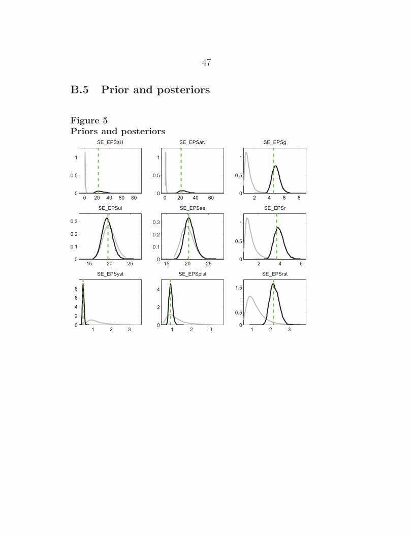
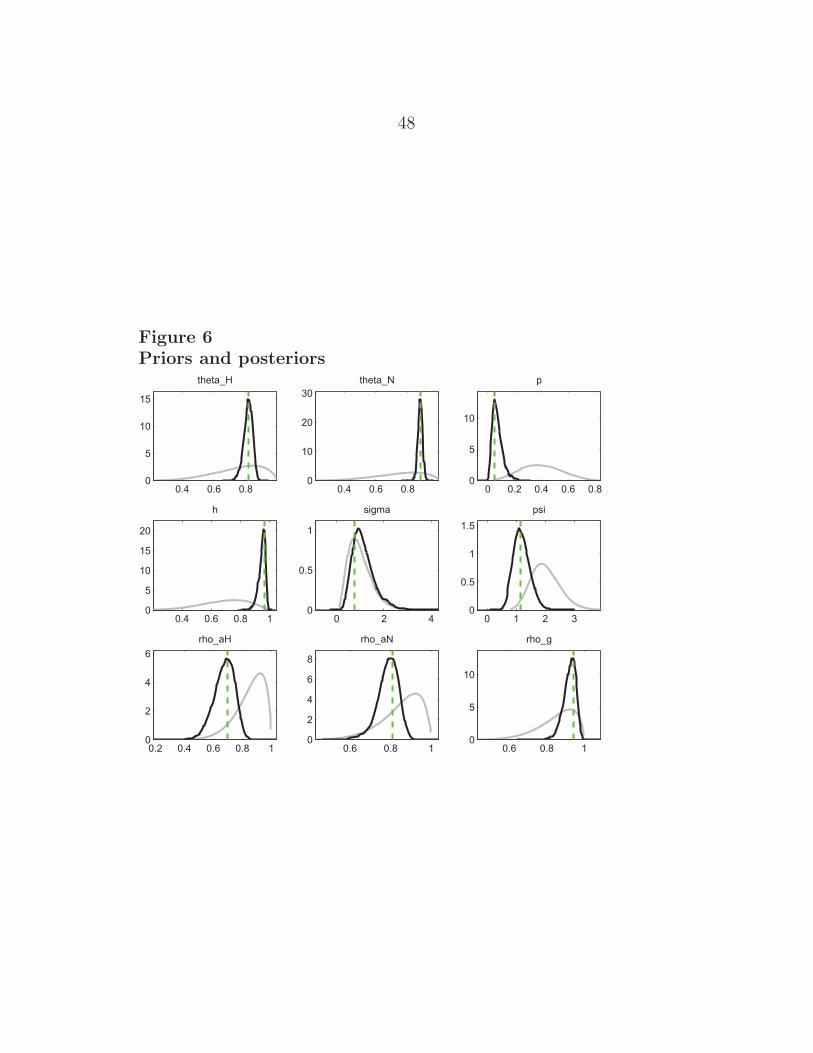
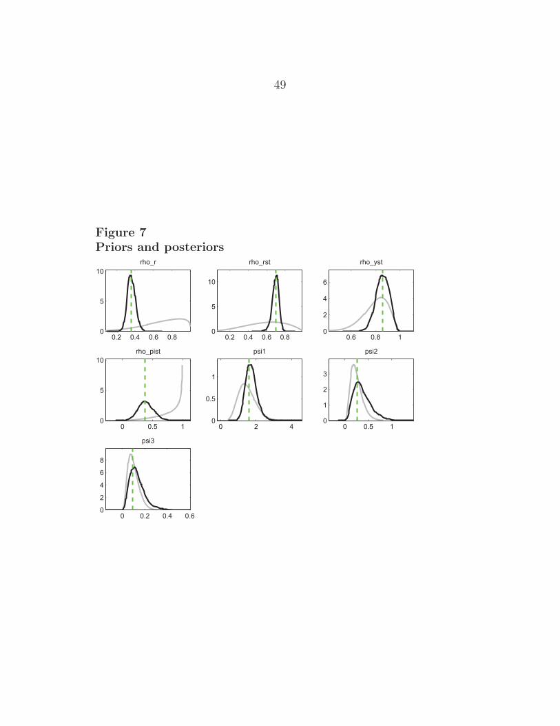
Priors and posteriors
Figures 5 to 7 represent the prior and posterior distributions of theparameters. The grey solid lines represent the prior distributions; thesolid black and dashed grey lines are the posterior distributions andtheir modes respectively. As can be seen, there are discrepancies be-tween the priors motivated by micro data and the posteriors that areinfluenced by macro data; see for example the habit persistence para-meter, the parameter indicating the proportion of firms that exhibitbackward-looking behaviour, and the degree of interest rate smoothing.In the rest of the cases, with some exceptions, the data are not veryinformative and the prior mode coincides with the posterior mode.In cases where the posterior distribution of the parameters is muchsharper (narrower) than the prior distribution, the data are very in-formative.
Parameter estimates
When I combine the joint prior distribution with the likelihood func-tion, I get a posterior density that cannot be evaluated analytically.In order to sample from the posterior, I employ a random walk chainMetropolis-Hasting algorithm where the proposal density is a multi-variate normal. I generate 150, 000 draws from the posterior distribu-tion, which is obtained using the Kalman filter.
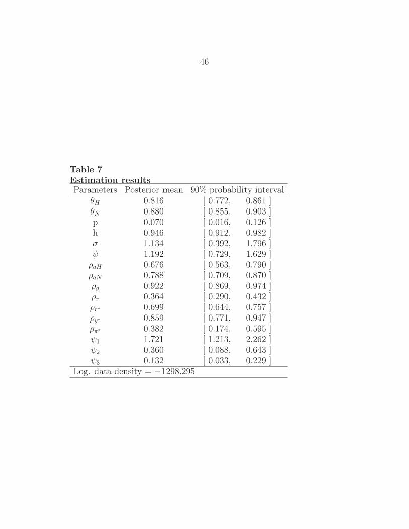
The parameter estimates are presented in table 7 in appendix B. As wecan see, there is a very high degree of price stickiness in both sectors,being higher in the home traded sector than in the non-traded sector.These results suggest that the degree of price rigidity is more importantin New Zealand than in the standard closed and large economies.

23
The autoregresive coefficients of the shocks are high, suggesting animportant degree of persistence driving the economy.
With respect to the parameters in the consumer’s utility function, theposterior estimates for the inverse of the elasticity of substitution, σ,and the inverse of the labour elasticity, ψ, are both lower than thosetypically found for large economies. The parameter representing habitpersistence is around 0.94, from which we can infer that consumers aremore concerned about consumption growth in the utility function thanabout the level.
The results do not suggest significant backward-looking behaviour inthe Phillips curve of both sectors. The relevant parameter, ω, is notsignificant, being around 0.07 (this suggests that the proportion offirms who behave in a backward-looking fashion is about 7 percent).16
If we analyze the value of the parameters in the reaction function, theresponse coefficient on inflation is 1.724. This implies that if inflationincreases by 1 percent, ceteris paribus, the Reserve Bank increases itsinterest rate by approximately 1.7 percent. The coefficient in front ofthe nominal exchange rate appreciation or depreciation is very small,around 0.10. This suggests that the RBNZ does not react strongly toexchange rate movements. The estimated coefficient for the reaction tooutput growth is 0.36, coherent with estimates in the literature. Lastly,the coefficient indicating interest rate smoothing is around 0.364, lowerthan the prior mean.
I perform a posterior odds test, which shows that the model with adirect response to overall inflation is better. I compare a model wherethe RBNZ responds to overall inflation with one where the RBNZresponds to non-tradable inflation. The posterior odds ratio is theratio of the posterior model probabilities.17 The log data density fromthe estimation is 1298.3.
16Note that I have assumed in the estimation procedure that the proportion of backward-lookingfirms is the same in both sectors, ie ωH=ωN=ω.
17More detail can be found in Koop (2003).
24
Consider the two models: Mi for i =‘o’, ‘n’, where ‘o’ refers to the nullof responding to overall inflation and ‘n’ refers to the reaction functionthat embodies a response to non-traded inflation. In this case,
POo,n =p(Mo|y)
p(Mn|y)=
p(y|Mo)p(Mo)
p(y|Mn)p(Mn)(78)
where p(y|Mi) is the marginal likelihood and p(Mi) is the prior modelprobability. If we assign the same prior probability to both models,the odds ratio is the ratio of the marginal likelihoods and is known asthe Bayes factor
BFo,n =p(y|Mo)
p(y|Mn)(79)
The greater the Bayes factor, the higher the support for Mo. In thepaper, BFo,n > 1. This means that the reaction function that respondsto overall inflation is supported by the evidence.
Impulse response analysis
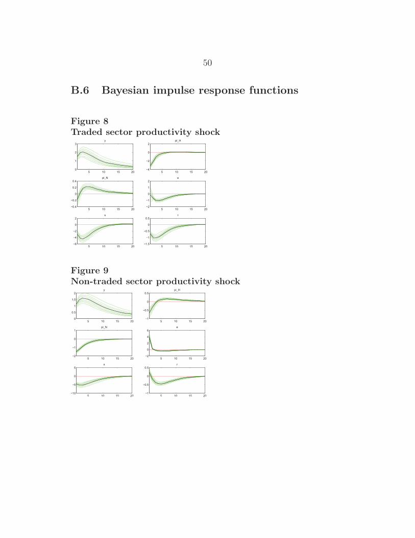
The impulse responses are generated from the reduced form represen-tation of the model. They represent the responses of the endogenousvariables to one-standard deviation shocks. Parameter uncertainty isincorporated in impulse-response analysis by constructing confidenceintervals for the model’s response to a shock. A full Bayesian impulseresponse function (IRF) analysis is presented.
In section B.6, I present the Bayesian impulse response functions cor-responding to the shocks of the economy. The confidence intervalsspan 95 percent of the probability mass. Figure 8 depicts a shock tothe traded goods sector. As we should expect, output increases andinflation in both sectors decreases (note that the reduction in inflationis higher in the sector that experiences the productivity improvement,the traded sector). The RBNZ reacts with an expansionary monetarypolicy and the nominal exchange rate depreciates. The terms of trade
25
fall, given the improvement in domestic productivity. Note the per-sistence of output, and that it returns to the steady state level, as weshould expect.
Figure 9 represents a productivity improvement in the non-tradedgoods sector. Again, output increases and inflation falls in both sec-tors. In contrast to the previous case, non-traded inflation declinesmore than in the traded sector, consistent with higher productivity inthe non-traded sector. The nominal exchange rate depreciates, giventhat the response of output is larger. The central bank is reacting moreto output growth than to deviations of inflation from the target.
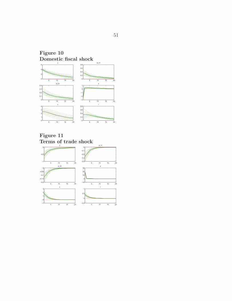
Figure 10 describes a domestic fiscal shock. This shock increases out-put and inflation in both sectors. The monetary authority contractsthe economy and the terms of trade increase, reflecting lower domesticproductivity. The higher interest rate appreciates the nominal ex-change rate.
A shock to the terms of trade is described in figure 11. This shockcauses an initial depreciation of the nominal exchange rate that de-creases output and inflation in both sectors. In contrast to what wewould expect, the monetary authority reacts by tightening the econ-omy, increasing the interest rate.
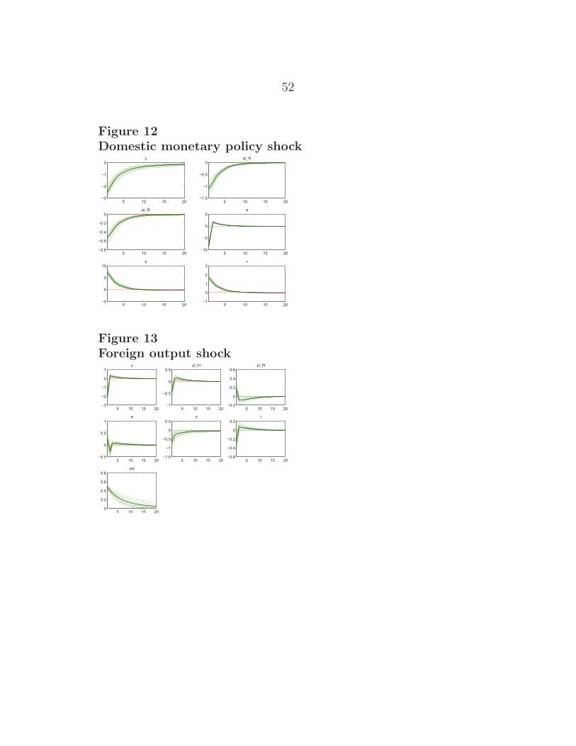
Figure 12 presents a contractionary domestic monetary policy shock.Output and inflation fall and the nominal exchange rate appreciates,as we should expect. The terms of trade increase initially, representinga worsening in domestic competitiveness.
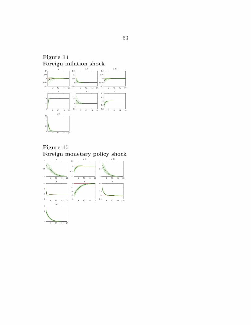
A negative foreign economy shock represented by a shock to foreignoutput (figure 13) or foreign inflation (figure 14) reduces domestic out-put. The negative foreign shock reduces the demand of domesticallyproduced goods and this reduces domestic output. In both cases, thecentral bank reacts by expanding the economy. In contrast, a con-tractionary foreign monetary policy shock increases domestic outputinitially and induces contractionary domestic monetary policy.
26
3.5 Comparison of empirical and model-based cross-
covariances
Following the procedure used in Smets and Wouters (2003), I vali-date the model by comparing the model-based variances and cross-covariances with those in the data. I calculate the cross-covariancesbetween the six observed data series implied by the model and comparethem with empirical cross-covariances. The empirical cross-covariancesare based on a VAR(2) estimated on the data sample covering the pe-riod 1992:Q1 to 2004:Q4. The model cross-covariances are also calcu-lated by estimating a VAR(2) on 10, 000 random samples of the obser-vations generated by the DSGE model. Generally the data covariances,for most of the 6 lags considered, fall within the error bands, suggest-ing that the model is able to mimic the cross-covariances of the data.The errors bands are very large: this suggests that there exists a largeamount of uncertainty surrounding the model-based cross-covariances.More detailed results and figures are available from the author uponrequest.
4 Alternative monetary policies
In the previous section, I estimated the model for the monetary pol-icy regime followed by New Zealand, where the central bank respondsdirectly to overall CPI inflation. In this section, I simulate the modelunder two alternative monetary policy regimes, and for different pref-erences of the central bank, and identify which reaction function min-imises the central bank’s loss function. The parameters are calibratedat the posterior mean of the estimated parameters in the previous sec-tion. The alternative reaction functions are:
rot = γo
1πt + γo2Δyt + γo
3rt−1 (80)
rNTt = γNT
1 πN,t + γNT2 Δyt + γNT
3 rt−1 (81)
27
The former invokes a direct response to overall inflation, whereas thelatter responds to non-tradables inflation.
To analyze the performance of the different monetary regimes, I followtwo procedures. First, I compare the volatility implied by the differentmonetary policy regimes on the variables that enter in the reactionfunction. Second, I simulate the model under both monetary policyregimes for different preferences of the central bank.
4.1 Volatility analysis
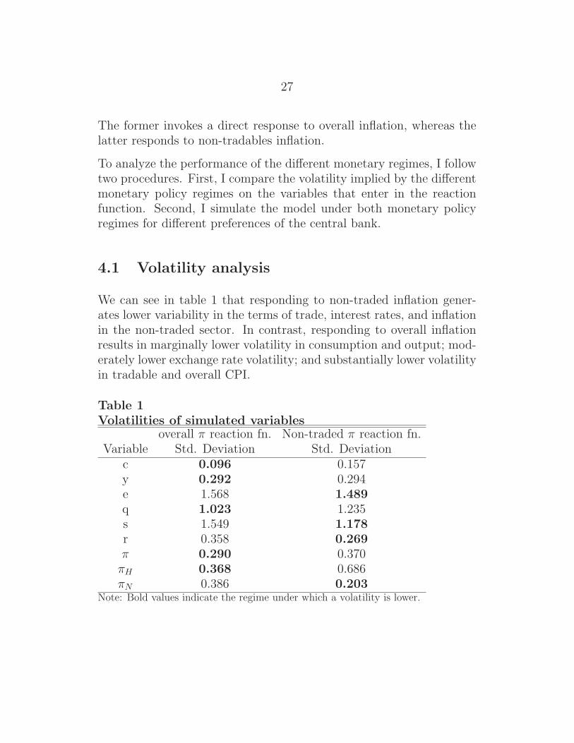
We can see in table 1 that responding to non-traded inflation gener-ates lower variability in the terms of trade, interest rates, and inflationin the non-traded sector. In contrast, responding to overall inflationresults in marginally lower volatility in consumption and output; mod-erately lower exchange rate volatility; and substantially lower volatilityin tradable and overall CPI.
Table 1Volatilities of simulated variables
overall π reaction fn. Non-traded π reaction fn.Variable Std. Deviation Std. Deviation
c 0.096 0.157y 0.292 0.294e 1.568 1.489q 1.023 1.235s 1.549 1.178r 0.358 0.269π 0.290 0.370πH 0.368 0.686πN 0.386 0.203
Note: Bold values indicate the regime under which a volatility is lower.
28
4.2 Should the RBNZ respond to non-traded in-
flation?
The volatility comparison above assumed that the central bank’s pref-erences were of a particular form. It is apparent from the volatilitycomparisons that the overall losses associated with the two reactionfunctions will depend on the weights applied to the various volatilities.
This subsection examines how the performance of the two reactionfunctions vary depending on the central bank’s preferences across in-flation, output, and interest rates. This experiment is a little differentto the direct comparison of volatilities because the reaction coefficientsare optimised for the central bank’s preferences. Given that the coeffi-cient on the exchange rate is small in the estimated reaction function,I set this coefficient to zero in the simulation.
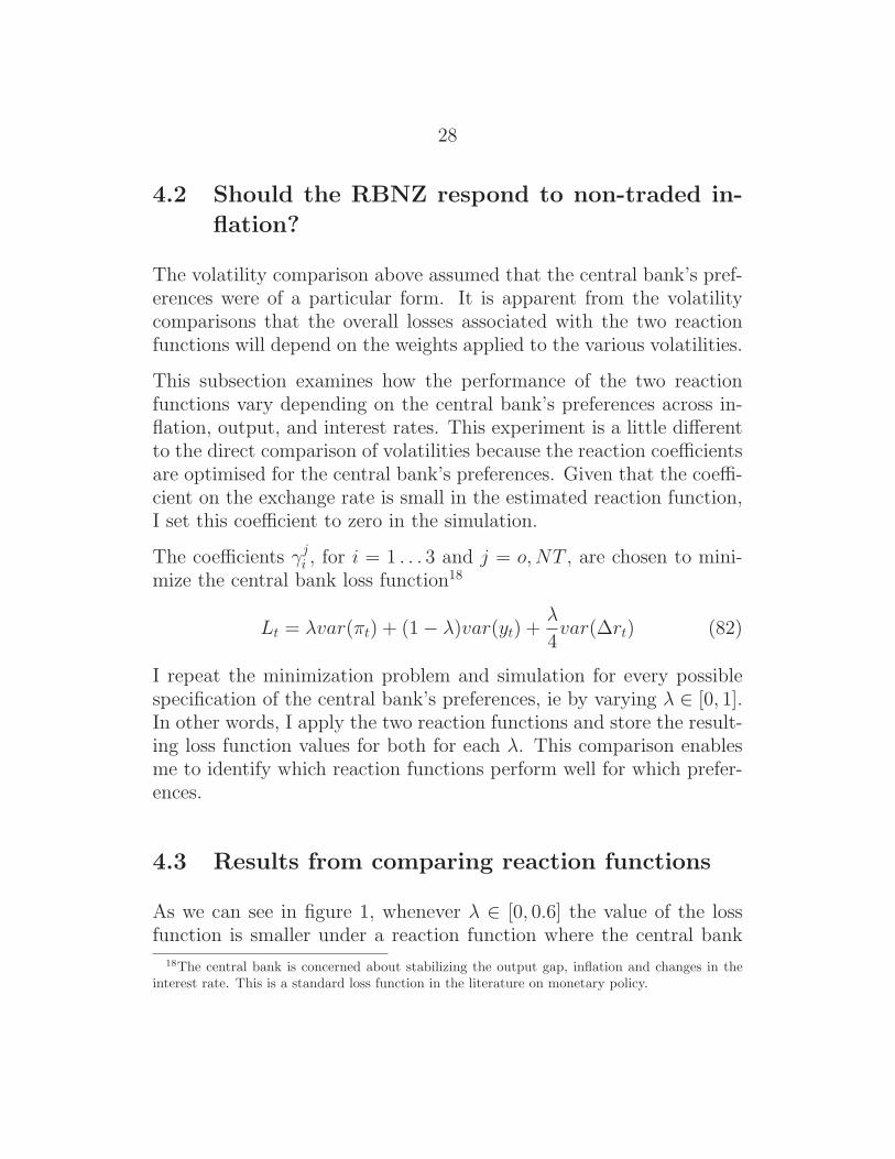
The coefficients γji , for i = 1 . . . 3 and j = o,NT , are chosen to mini-
mize the central bank loss function18
Lt = λvar(πt) + (1 − λ)var(yt) +λ
4var(Δrt) (82)
I repeat the minimization problem and simulation for every possiblespecification of the central bank’s preferences, ie by varying λ ∈ [0, 1].In other words, I apply the two reaction functions and store the result-ing loss function values for both for each λ. This comparison enablesme to identify which reaction functions perform well for which prefer-ences.
4.3 Results from comparing reaction functions
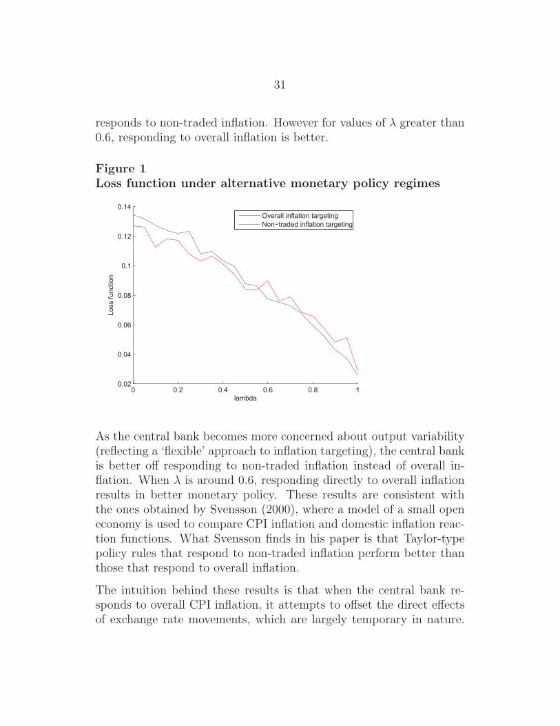
As we can see in figure 1, whenever λ ∈ [0, 0.6] the value of the lossfunction is smaller under a reaction function where the central bank
18The central bank is concerned about stabilizing the output gap, inflation and changes in theinterest rate. This is a standard loss function in the literature on monetary policy.
29
Table 2overall inflation reaction function lossesλ Loss Value γ1 γ2 γ3
0 0.134 1.56 0.86 0.600.05 0.132 1.23 0.86 0.600.10 0.127 1.12 0.95 10.15 0.124 1.01 0.95 0.530.20 0.122 1.56 0.76 0.670.25 0.124 1.23 0.86 0.670.30 0.108 1.12 0.86 10.35 0.110 1.23 0.86 0.930.40 0.103 1.12 0.95 10.45 0.100 1.12 0.57 0.800.50 0.088 1.67 0.76 10.55 0.086 1.56 0.95 0.870.60 0.078 1.01 0.57 0.730.65 0.075 1.56 0.95 0.930.70 0.073 1.23 0.48 0.870.75 0.068 1.12 0.76 10.80 0.060 1.01 0.38 10.85 0.052 1.12 0.48 10.90 0.043 1.23 0.38 10.95 0.037 1.23 0.29 11 0.026 1.23 0.10 0.93
30
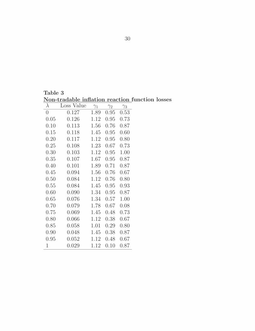
Table 3Non-tradable inflation reaction function lossesλ Loss Value γ1 γ2 γ3
0 0.127 1.89 0.95 0.530.05 0.126 1.12 0.95 0.730.10 0.113 1.56 0.76 0.870.15 0.118 1.45 0.95 0.600.20 0.117 1.12 0.95 0.800.25 0.108 1.23 0.67 0.730.30 0.103 1.12 0.95 1.000.35 0.107 1.67 0.95 0.870.40 0.101 1.89 0.71 0.870.45 0.094 1.56 0.76 0.670.50 0.084 1.12 0.76 0.800.55 0.084 1.45 0.95 0.930.60 0.090 1.34 0.95 0.870.65 0.076 1.34 0.57 1.000.70 0.079 1.78 0.67 0.080.75 0.069 1.45 0.48 0.730.80 0.066 1.12 0.38 0.670.85 0.058 1.01 0.29 0.800.90 0.048 1.45 0.38 0.870.95 0.052 1.12 0.48 0.671 0.029 1.12 0.10 0.87
31
responds to non-traded inflation. However for values of λ greater than0.6, responding to overall inflation is better.
Figure 1Loss function under alternative monetary policy regimes
0 0.2 0.4 0.6 0.8 10.02
0.04
0.06
0.08
0.1
0.12
0.14
lambda
Loss
func
tion
Overall inflation targetingNon−traded inflation targeting
As the central bank becomes more concerned about output variability(reflecting a ‘flexible’ approach to inflation targeting), the central bankis better off responding to non-traded inflation instead of overall in-flation. When λ is around 0.6, responding directly to overall inflationresults in better monetary policy. These results are consistent withthe ones obtained by Svensson (2000), where a model of a small openeconomy is used to compare CPI inflation and domestic inflation reac-tion functions. What Svensson finds in his paper is that Taylor-typepolicy rules that respond to non-traded inflation perform better thanthose that respond to overall inflation.
The intuition behind these results is that when the central bank re-sponds to overall CPI inflation, it attempts to offset the direct effectsof exchange rate movements, which are largely temporary in nature.
32
When the exchange rate depreciates, the perfect pass-through causesCPI inflation to rise over the very short-term. In response, monetarypolicy increases interest rates, which causes the exchange rate to appre-ciate and a fall in CPI inflation. Monetary policy then has to contendwith the indirect exchange rate impact via the exchange rate effect onthe output gap. In contrast, when the central bank responds directlyto non-traded inflation, it ignores the direct exchange rate impact onCPI and instead focuses on the direct effect via the output gap.19
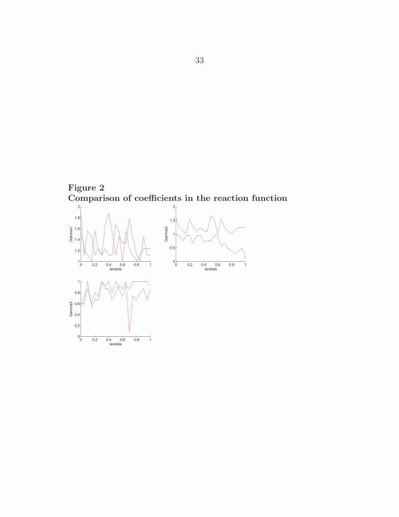
All these results are reinforced in figure 2. As we can see in the rightupper graph, representing the coefficients of the reaction functions,the central bank reacts more strongly to deviations of overall inflationfrom its desired level than when the central bank is responding tonon-traded inflation. The opposite happens with the output gap (leftupper graph). In the case of interest rate smoothing, neither reactionfunction dominates when λ ≤ 0.6. Nevertheless, for values of λ ≥ 0.6,the loss is lower when the central bank responds directly to non-tradedinflation rather than overall inflation.
19These results were found by Conway, Drew, Hunt and Scott (1998) who address the samequestion with a less structural model.
33
Figure 2Comparison of coefficients in the reaction function
0 0.2 0.4 0.6 0.8 11
1.2
1.4
1.6
1.8
2
Gam
ma1
lambda0 0.2 0.4 0.6 0.8 1
0
0.5
1
1.5
2
lambda
Gam
ma2
0 0.2 0.4 0.6 0.8 10
0.2
0.4
0.6
0.8
1
lambda
Gam
ma3
34
5 Conclusions
Should the central bank of a small open economy respond to overallCPI inflation? Or should it take into account the multisectoral struc-ture of the economy? To respond to those questions, I have analysed astructural general equilibrium model of a small open economy with twosectors: a traded sector and a non-traded sector. The model sharesthe characteristics of the new open economy models, adapted to repre-sent the features of the New Zealand economy. In particular, I assumea loss function where the central bank is concerned about inflation,output growth and exchange rate movements.
From the estimation of the model, I obtain the characteristics of theNew Zealand economy, given by the posterior means of the parameters.New Zealand is an economy characterized by a high degree of pricestickiness, low inverse elasticities of intertemporal and intratemporalsubstitution in the utility function, and a very high degree of habitpersistence. The evidence suggests that the central bank respondsdirectly to overall CPI inflation (cf non-tradable inflation) and thatthe direct reaction to exchange rate movements is not very important.
Taking into account these characteristics, I have obtained conditionsunder which the central bank would minimize losses by following a re-action function with a direct response to non-traded inflation, insteadof the actual policy rule of responding to overall CPI inflation. Theresults in the paper show that the choice of reaction function dependson the central bank’s preferences. In particular, if preferences are rel-atively biased towards inflation stabilization, responding directly tooverall inflation is better. If instead the central bank places relativelymore weight on output stabilization, responding directly to non-tradedinflation is a better strategy. These results, however, do not take intoaccount uncertainty in the parameters. This uncertainty should betaken into account in future research, by introducing Bayesian calibra-tion in the simulation of the different monetary policy regimes.
35
References
Bharucha, N and C Kent (1998), “Inflation targeting in a small openeconomy,” Reserve Bank of Australia Research Discussion Paper,RDP9802.
Boldrin, M, L J Christiano, and J D M Fisher (2001), “Habit pre-sistence, asset returns and the business cycle,” American Eco-nomic Review, 91(1), 149–66.
Conway, P, A Drew, B Hunt, and A Scott (1998), “Exchange rate ef-fects and inflation targeting in a small open economy: A stochas-tic analysis using FPS,” Reserve Bank of New Zealand Discussionpaper, G99/4.
Corsetti, G, L Dedola, and S Leduc (2005), “International risk-sharingand the transmission of productivity shocks,” Board of Gover-nors of the Federal Reserve System (U.S.), International FinanceDiscussion Papers, 826.
Deaton, A and J Muellbauer (1980), “An almost ideal demand sys-tem,” American Economic Review, 70(3), 312–26.
Duesenberry, J S (1949), Income, Saving and Theory of ConsumerBehaviour, Harvard University Press, Cambridge, MA.
Fuhrer, J (2000), “Habit formation in consumption and its implicationsfor monetary-policy models,” American Economic Review, 90(3),367–90.
Gali, J and M Gertler (1999), “Inflation dynamics: A structural econo-metric analysis,” Journal of Monetary Economics, 44(2), 195–222.
Gali, J and T Monacelli (2005), “Optimal monetary policy and ex-change rate volatility in a small open economy,” Review of Eco-nomic Studies, forthcoming.
36
Geweke, J (1999), “Using simulation methods for Bayesian econometricmodels: Inference, development and communication,” Economet-ric Reviews, 18(1), 1–73.
Koop, G (2003), Bayesian Econometrics, John Wiley and Sons, Ltd,Chichester, England.
Lettau, M and H Uhlig (2000), “Can habit formation be reconciledwith business cycle facts?” Review of Economic Dynamics, 3(1),79–99.
Lubik, T (2003), “Industrial structure and monetary policy in a smallopen economy,” The Johns Hopkins University, Department ofEconomics Working Paper, 493.
Lubik, T and F Schorfheide (2003), “Do central banks respond toexchange rate movements? A structural investigation,” The JohnsHopkins University, Department of Economics Working Paper,505.
Lubik, T and F Schorfheide (2005), “A Bayesian look at newopen economy macroeconomics,” The Johns Hopkins Univer-sity,Department of Economics Working Paper, 521.
Obstfeld, M and K Rogoff (2000), “New directions for stochastic openeconomy models,” Journal of International Economics, 50(1),117–53.
Ortega, E and N Rebei (2005), “The welfare implications of inflationversus price-level targeting in a two-sector, small open economy,”Bank of Canada Mimeo, presented at “Issues in Inflation Target-ing” Conference, Bank of Canada, 28–29 April 2005.
RBNZ (2005), Reserve Bank of New Zealand Monetary Policy State-ment, http://www.rbnz.govt.nz/monpol/statements/index.html.
Schorfheide, F (2000), “Loss function-based evaluation of DSGE mod-els,” Journal of Applied Econometrics, 15(6), 645–70.
37
Smets, F and R Wouters (2002), “An estimated stochastic dynamicgeneral equilibrium model of the euro area,” European CentralBank Working Paper, 171.
Smets, F and R Wouters (2003), “An estimated stochastic dynamicgeneral equilibrium model of the euro area,” Journal of the Euro-pean Economic Association, 1(5), 1123–1175.
Svensson, L (2000), “Open-economy inflation targeting,” Journal ofInternational Economics, 50(1), 155–83.

38
Appendices
A Motivation
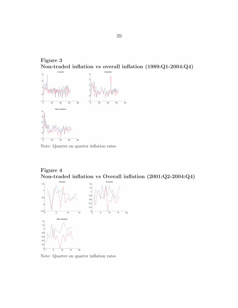
The following table presents variance, covariance and correlation coef-ficients of non-traded inflation and overall inflation for Canada, Aus-tralia and New Zealand (period 1989:Q1 to 2004:Q4).
Table 4Moments of inflation series (part A)
Country Canada Australia New ZealandVariance Non-tradable CPI 0.306 0.252 0.351Variance CPI 0.1410 0.509 0.330Covariance 0.136 0.172 0.259Correlation Coefficient 0.654 0.500 0.760
The following table presents variance, covariance and correlation coef-ficients of non-traded inflation and overall inflation for Canada, Aus-tralia and New Zealand (period 2001:Q2 to 2004:Q4).
Table 5Moments of inflation series (part B)
Country Canada Australia New ZealandVariance Non-tradable CPI 0.173 0.092 0.074Variance CPI 0.250 0.086 0.061Covariance 0.115 0.016 -0.016Correlation Coefficient 0.556 0.178 -0.237
39
Figure 3Non-traded inflation vs overall inflation (1989:Q1-2004:Q4)
0 20 40 60 80−1
0
1
2
3Canada
0 20 40 60 80−1
0
1
2
3
4Australia
0 20 40 60 80−1
0
1
2
3
4New Zealand
Note: Quarter on quarter inflation rates
Figure 4Non-traded inflation vs Overall inflation (2001:Q2-2004:Q4)
0 5 10 15−0.5
0
0.5
1
1.5Canada
0 5 10 15 200
0.2
0.4
0.6
0.8
1
1.2
1.4Australia
0 5 10 15 200
0.2
0.4
0.6
0.8
1
1.2
1.4New Zealand
Note: Quarter on quarter inflation rates
40
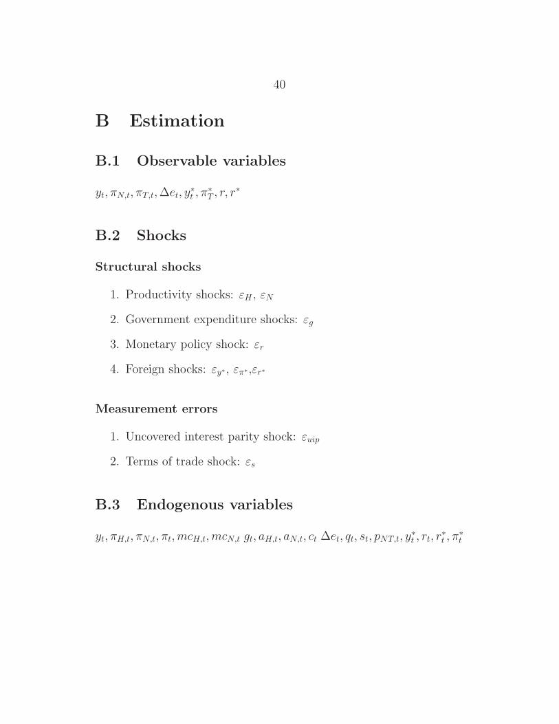
B Estimation
B.1 Observable variables
yt, πN,t, πT,t, Δet, y∗t , π
∗T , r, r∗
B.2 Shocks
Structural shocks
1. Productivity shocks: εH , εN
2. Government expenditure shocks: εg
3. Monetary policy shock: εr
4. Foreign shocks: εy∗, επ∗,εr∗
Measurement errors
1. Uncovered interest parity shock: εuip
2. Terms of trade shock: εs
B.3 Endogenous variables
yt, πH,t, πN,t, πt,mcH,t,mcN,t gt, aH,t, aN,t, ct Δet, qt, st, pNT,t, y∗t , rt, r
∗t , π
∗t
41
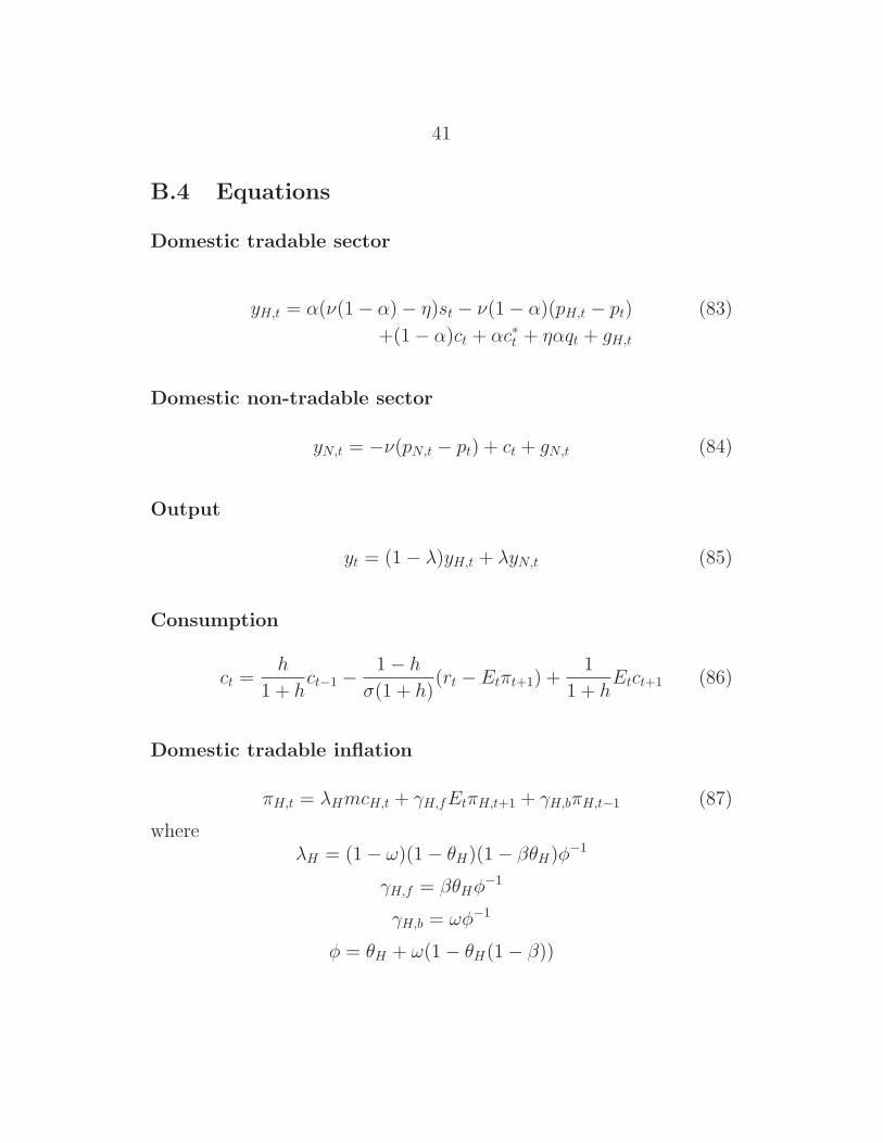
B.4 Equations
Domestic tradable sector
yH,t = α(ν(1 − α) − η)st − ν(1 − α)(pH,t − pt) (83)
+(1 − α)ct + αc∗t + ηαqt + gH,t
Domestic non-tradable sector
yN,t = −ν(pN,t − pt) + ct + gN,t (84)
Output
yt = (1 − λ)yH,t + λyN,t (85)
Consumption
ct =h
1 + hct−1 − 1 − h
σ(1 + h)(rt − Etπt+1) +
1
1 + hEtct+1 (86)
Domestic tradable inflation
πH,t = λHmcH,t + γH,fEtπH,t+1 + γH,bπH,t−1 (87)
whereλH = (1 − ω)(1 − θH)(1 − βθH)φ−1
γH,f = βθHφ−1
γH,b = ωφ−1
φ = θH + ω(1 − θH(1 − β))
42
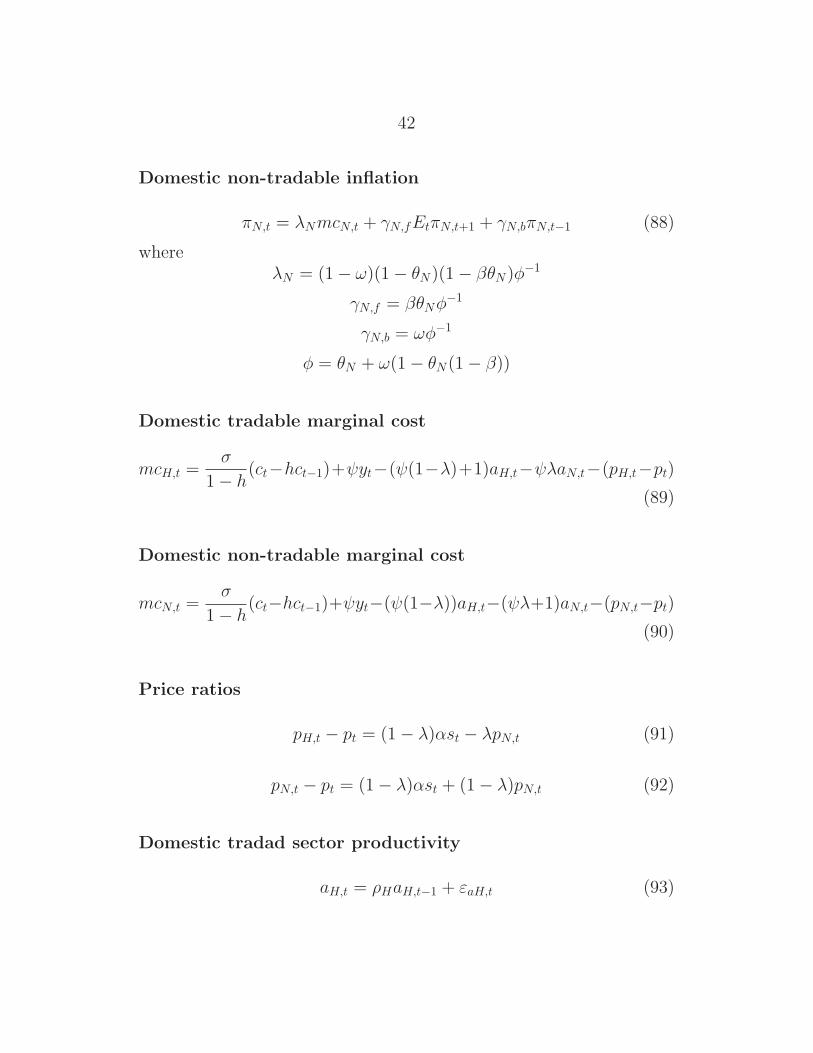
Domestic non-tradable inflation
πN,t = λNmcN,t + γN,fEtπN,t+1 + γN,bπN,t−1 (88)
whereλN = (1 − ω)(1 − θN)(1 − βθN)φ−1
γN,f = βθNφ−1
γN,b = ωφ−1
φ = θN + ω(1 − θN(1 − β))
Domestic tradable marginal cost
mcH,t =σ
1 − h(ct−hct−1)+ψyt−(ψ(1−λ)+1)aH,t−ψλaN,t−(pH,t−pt)
(89)
Domestic non-tradable marginal cost
mcN,t =σ
1 − h(ct−hct−1)+ψyt−(ψ(1−λ))aH,t−(ψλ+1)aN,t−(pN,t−pt)
(90)
Price ratios
pH,t − pt = (1 − λ)αst − λpN,t (91)
pN,t − pt = (1 − λ)αst + (1 − λ)pN,t (92)
Domestic tradad sector productivity
aH,t = ρHaH,t−1 + εaH,t (93)
43
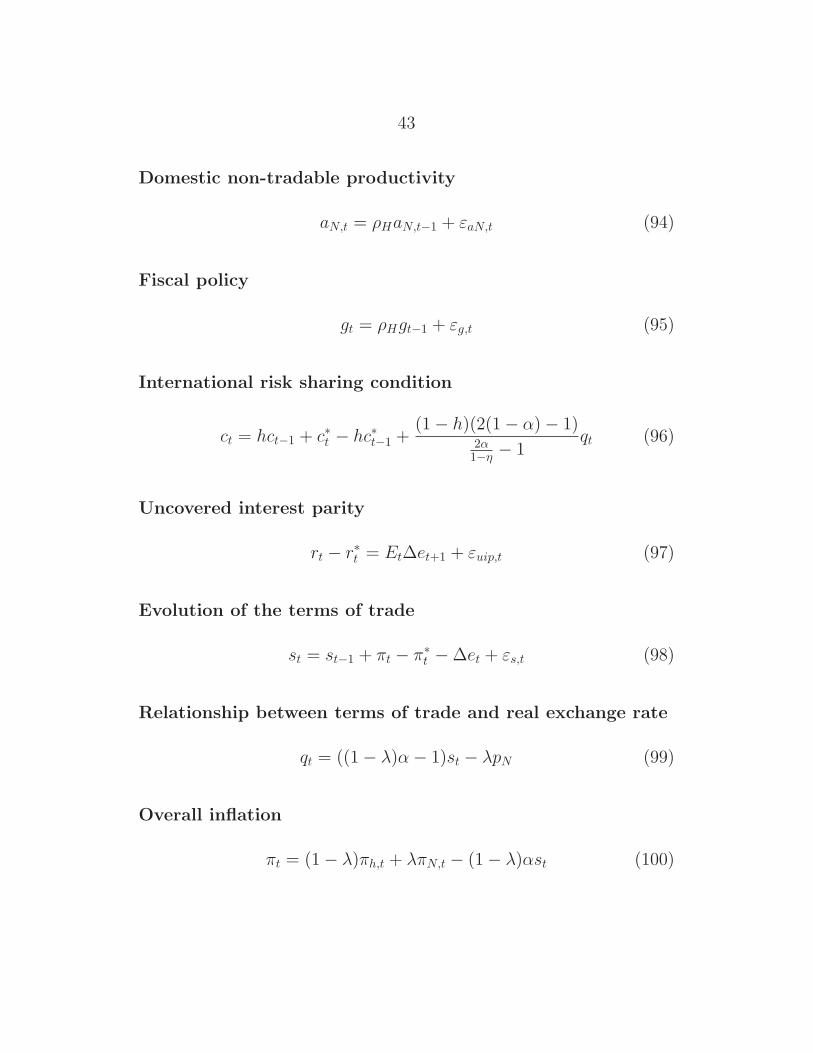
Domestic non-tradable productivity
aN,t = ρHaN,t−1 + εaN,t (94)
Fiscal policy
gt = ρHgt−1 + εg,t (95)
International risk sharing condition
ct = hct−1 + c∗t − hc∗t−1 +(1 − h)(2(1 − α) − 1)
2α1−η − 1
qt (96)
Uncovered interest parity
rt − r∗t = EtΔet+1 + εuip,t (97)
Evolution of the terms of trade
st = st−1 + πt − π∗t − Δet + εs,t (98)
Relationship between terms of trade and real exchange rate
qt = ((1 − λ)α − 1)st − λpN (99)
Overall inflation
πt = (1 − λ)πh,t + λπN,t − (1 − λ)αst (100)
44
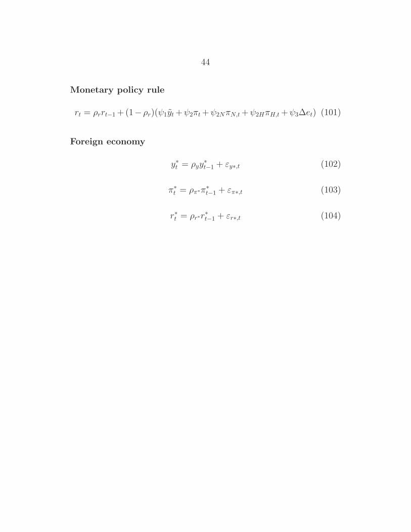
Monetary policy rule
rt = ρrrt−1 +(1− ρr)(ψ1yt +ψ2πt +ψ2NπN,t +ψ2HπH,t +ψ3Δet) (101)
Foreign economy
y∗t = ρyy∗t−1 + εy∗,t (102)
π∗t = ρπ∗π∗
t−1 + επ∗,t (103)
r∗t = ρr∗r∗t−1 + εr∗,t (104)
45
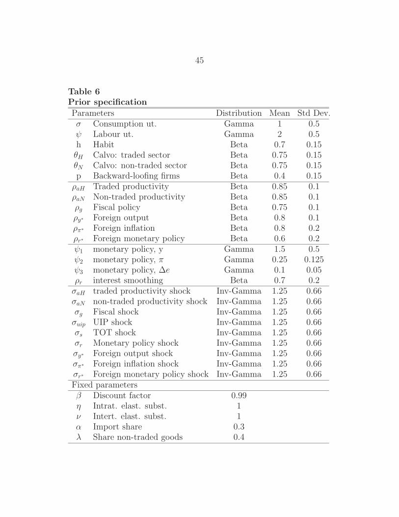
Table 6Prior specification
Parameters Distribution Mean Std Dev.σ Consumption ut. Gamma 1 0.5ψ Labour ut. Gamma 2 0.5h Habit Beta 0.7 0.15θH Calvo: traded sector Beta 0.75 0.15θN Calvo: non-traded sector Beta 0.75 0.15p Backward-loofing firms Beta 0.4 0.15
ρaH Traded productivity Beta 0.85 0.1ρaN Non-traded productivity Beta 0.85 0.1ρg Fiscal policy Beta 0.75 0.1ρy∗ Foreign output Beta 0.8 0.1ρπ∗ Foreign inflation Beta 0.8 0.2ρr∗ Foreign monetary policy Beta 0.6 0.2ψ1 monetary policy, y Gamma 1.5 0.5ψ2 monetary policy, π Gamma 0.25 0.125ψ3 monetary policy, Δe Gamma 0.1 0.05ρr interest smoothing Beta 0.7 0.2
σaH traded productivity shock Inv-Gamma 1.25 0.66σaN non-traded productivity shock Inv-Gamma 1.25 0.66σg Fiscal shock Inv-Gamma 1.25 0.66σuip UIP shock Inv-Gamma 1.25 0.66σs TOT shock Inv-Gamma 1.25 0.66σr Monetary policy shock Inv-Gamma 1.25 0.66σy∗ Foreign output shock Inv-Gamma 1.25 0.66σπ∗ Foreign inflation shock Inv-Gamma 1.25 0.66σr∗ Foreign monetary policy shock Inv-Gamma 1.25 0.66Fixed parametersβ Discount factor 0.99η Intrat. elast. subst. 1ν Intert. elast. subst. 1α Import share 0.3λ Share non-traded goods 0.4
46
Table 7Estimation resultsParameters Posterior mean 90% probability interval
θH 0.816 [ 0.772, 0.861 ]θN 0.880 [ 0.855, 0.903 ]p 0.070 [ 0.016, 0.126 ]h 0.946 [ 0.912, 0.982 ]σ 1.134 [ 0.392, 1.796 ]ψ 1.192 [ 0.729, 1.629 ]
ρaH 0.676 [ 0.563, 0.790 ]ρaN 0.788 [ 0.709, 0.870 ]ρg 0.922 [ 0.869, 0.974 ]ρr 0.364 [ 0.290, 0.432 ]ρr∗ 0.699 [ 0.644, 0.757 ]ρy∗ 0.859 [ 0.771, 0.947 ]ρπ∗ 0.382 [ 0.174, 0.595 ]ψ1 1.721 [ 1.213, 2.262 ]ψ2 0.360 [ 0.088, 0.643 ]ψ3 0.132 [ 0.033, 0.229 ]
Log. data density = −1298.295
47
B.5 Prior and posteriors
Figure 5Priors and posteriors
0 20 40 60 800
0.5
1
SE_EPSaH
0 20 40 600
0.5
1
SE_EPSaN
2 4 6 80
0.5
1
SE_EPSg
15 20 250
0.1
0.2
0.3
SE_EPSui
15 20 250
0.1
0.2
0.3
SE_EPSee
2 4 60
0.5
1
SE_EPSr
1 2 30
2
4
6
8
SE_EPSyst
1 2 30
2
4
SE_EPSpist
1 2 30
0.5
1
1.5
SE_EPSrst
48
Figure 6Priors and posteriors
0.4 0.6 0.80
5
10
15
theta_H
0.4 0.6 0.80
10
20
30theta_N
0 0.2 0.4 0.6 0.80
5
10
p
0.4 0.6 0.8 10
5
10
15
20
h
0 2 40
0.5
1
sigma
0 1 2 30
0.5
1
1.5psi
0.2 0.4 0.6 0.8 10
2
4
6rho_aH
0.6 0.8 10
2
4
6
8
rho_aN
0.6 0.8 10
5
10
rho_g
49
Figure 7Priors and posteriors
0.2 0.4 0.6 0.80
5
10rho_r
0.2 0.4 0.6 0.80
5
10
rho_rst
0.6 0.8 10
2
4
6
rho_yst
0 0.5 10
5
10rho_pist
0 2 40
0.5
1
psi1
0 0.5 10
1
2
3
psi2
0 0.2 0.4 0.60
2
4
6
8
psi3
50
B.6 Bayesian impulse response functions
Figure 8Traded sector productivity shock
5 10 15 200
1
2
3y
5 10 15 20−4
−2
0
2pi_H
5 10 15 20−0.4
−0.2
0
0.2
0.4pi_N
5 10 15 20−2
−1
0
1
2e
5 10 15 20−6
−4
−2
0
2s
5 10 15 20−1.5
−1
−0.5
0
0.5r
Figure 9Non-traded sector productivity shock
5 10 15 200
0.5
1
1.5
2y
5 10 15 20−1
−0.5
0
0.5pi_H
5 10 15 20−2
−1
0
1pi_N
5 10 15 20−2
0
2
4
6e
5 10 15 20−10
−5
0
5s
5 10 15 20−1
−0.5
0
0.5r
51
Figure 10Domestic fiscal shock
5 10 15 200
2
4
6y
5 10 15 200
0.2
0.4
0.6
0.8pi_H
5 10 15 200
0.1
0.2
0.3
0.4pi_N
5 10 15 20−3
−2
−1
0
1e
5 10 15 200
1
2
3
4s
5 10 15 200
0.2
0.4
0.6
0.8r
Figure 11Terms of trade shock
5 10 15 20−1
−0.5
0y
5 10 15 20−0.4
−0.3
−0.2
−0.1
0pi_H
5 10 15 20−0.2
−0.15
−0.1
−0.05
0pi_N
5 10 15 20−10
0
10
20
30e
5 10 15 20−1
0
1
2
3s
5 10 15 20−0.5
0
0.5
1r
52
Figure 12Domestic monetary policy shock
5 10 15 20−3
−2
−1
0y
5 10 15 20−1.5
−1
−0.5
0pi_H
5 10 15 20−0.8
−0.6
−0.4
−0.2
0pi_N
5 10 15 20−10
−5
0
5e
5 10 15 20−5
0
5
10s
5 10 15 20−1
0
1
2
3r
Figure 13Foreign output shock
5 10 15 20−3
−2
−1
0
1y
5 10 15 20−1
−0.5
0
0.5pi_H
5 10 15 20−0.2
0
0.2
0.4
0.6pi_N
5 10 15 20−0.5
0
0.5
1e
5 10 15 20−1.5
−1
−0.5
0
0.5s
5 10 15 20−0.6
−0.4
−0.2
0
0.2r
5 10 15 200
0.2
0.4
0.6
0.8yst
53
Figure 14Foreign inflation shock
5 10 15 20−0.1
−0.05
0
0.05
0.1y
5 10 15 20−0.05
0
0.05
0.1
0.15pi_H
5 10 15 20−0.1
−0.05
0
0.05
0.1pi_N
5 10 15 20−2
−1
0
1e
5 10 15 20−0.5
0
0.5
1s
5 10 15 20−0.2
−0.1
0
0.1
0.2r
5 10 15 200
0.5
1
1.5pist
Figure 15Foreign monetary policy shock
5 10 15 200
0.5
1y
5 10 15 20−1
−0.5
0
0.5pi_H
5 10 15 200
0.5
1pi_N
5 10 15 20−5
0
5
10e
5 10 15 20−8
−6
−4
−2
0s
5 10 15 20−0.5
0
0.5
1
1.5r
5 10 15 200
1
2
3rst