Embed Size (px)
Citation preview
REACHABLE SET CONTROLFOR
PREFERRED AXIS HOMING MISSILES
By
DONALD J. CAUGHLIN, JR.
A DISSERTATION PRESENTED TO THE GRADUATE SCHOOLOF THE UNIVERSITY OF FLORIDA IN
PARTIAL FULFILLMENT OF THE REQUIREMENTSFOR THE DEGREE OF DOCTOR OF PHILOSOPHY
UNIVERSITY OF FLORIDA
1988
Copyright 1988
By
DONALD J. CAUGHLIN JR.
To Barbara
Amy
Jon
ACKNOWLEDGMENTS
The author wishes to express his gratitude to his committee chairman, Dr.
T.E Bullock, for his instruction, helpful suggestions, and encouragement.
Appreciation is also expressed for the support and many helpful comments from
the other committee members, Dr. Basile, Dr. Couch, Dr. Smith, and Dr. Svoronos.
iv
TABLE OF CONTENTS
ACKNOWLEDGMENTS iv
LIST OF FIGURES vii
KEY TO SyMBOLS ix
ABSTRACT xiv
CHAPTER
I INTRODUCTION 1
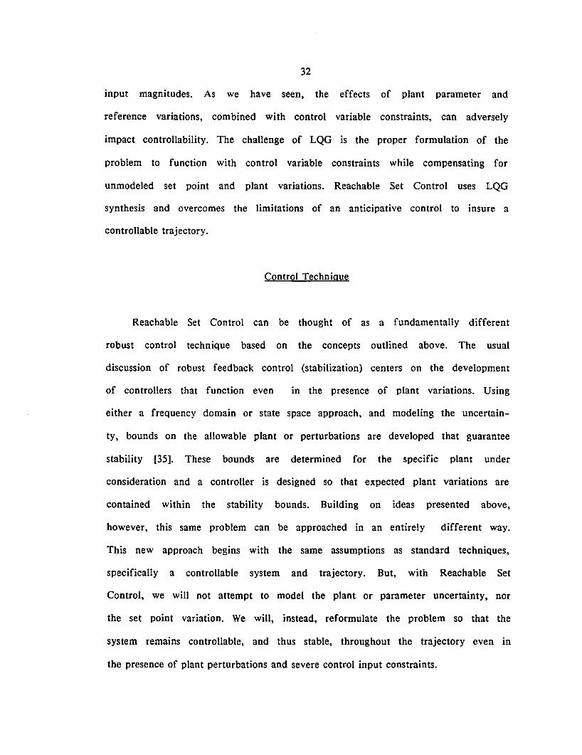
II BACKGROUND 4Missile Dynamics 5
Linear Accelerations 6Moment Equations (i
Linear Quadratic Gaussian Control Law 7
III CONSTRAINED CONTROL 13
IV CONSTRAINED CONTROL WITH UNMODELED SETPOINTAND PLANT VARIATIONS 25
Linear Optimal Control with Uncertainty and Constraints 31Control Technique 32Discussion 36Procedure .37
V REACHABLE SET CONTROL EXAMPLE .41Performance Comparison - Reachable Set and LQG Control... .41Summary .54
VI REACHABLE SET CONTROL FOR PREFERRED AXISHOMING MISSILES 55
Acceleration Control. 56System Model. 56Disturbance Model 58Reference Model. 60
Roll Control. 62Definition 62Controller 66
Kalman FiIter 67Reachable Set Controller 68
Structure 68Application 72
v
VII RESULTS AND DISCUSSION 76Simulation 77
Trajectory Parameters 78Results 78
Deterministic Results 78Stochastic Results 81
Conclusions 87Reachable Set Control. 87Singer Model. 87
APPENDIX
A SIMULATION RESULTS 88
B SAMPLED-DATA CONVERSION 94System Model 94Sampled Data Equations 96
System 96Target Disturbance 98Minimum Control Reference 99
Summary 100
C SAMPLED DATA COST FUNCTIONS 101
D LQG CONTROLLER DECOMPOSITION .1 07
E CONTROLLER PARAMETERS 111Control Law 111Filter 112
LIST OF REFERENCES 113
BIOGRAPHICAL SKETCH 117
vi
LIST OF FIGURES
Figure Page
2.1 Missile Reference System 4
4.1 Feedback System and Notation 28
4.2 Reachable Set Control Objective 33
4.3 Intersection of Missile Reachable Sets Based onUncertain Target Motion and Symmetric Constraints .38
4.4 Intersection of Missile Reachable Sets Based onUncertain Target Motion andUnsymmetric Constraints 38
5.1 Terminal Performance of Linear Optimal Control.. .43
5.2 Initial Acceleration of Linear Optimal Control. 43
5.3 Linear Optimal Acceleration vs Time 45
5.4 Linear Optimal Velocity vs Time 45
5.5 Linear Optimal Position vs Time lt6
5.6 Unconstrained and Constrained Acceleration .47
5.7 Unconstrained and Constrained Velocity vs Time .48
5.8 Unconstrained and Constrained Position vs Time .48
5.9 Acceleration ProfileWith and Without Target Set Uncertainty 50
5.10 Velocity vs TimeWith and Without Target Set Uncertainty 50
5.11 Position vs TimeWith and Without Target Set Uncertainty 51
5.12 Acceleration vs TimeLQG and Reachable Set Control. 52
vii
5.13 Velocity vs TimeLQG and Reachable Set Control. 53
5.14 Position vs TimeLQG and Reachable Set Control. 53
6.1 Reachable Set Control Disturbance processes 60
6.2. Roll Angle Error Definition from Seeker Angles 63
6.3. Roll Control Zones 65
6.4 Target Missile System 74
6.5 Command Generator/Tracker 75
7.1 RMS Missile Acceleration 76
7.2 Engagement Geometry 77
7.3 Deterministic Results 80
7.4 Stochastic Results 81
7.5 Measured vs Actual Z Axis Velocity 84
7.6 Performance Using Position Estimatesand Actual Velocities 86
A.I XY Missile & Target PositionsReachable Set Control. 89
A.2 XY Missile & Target PositionsBaseline Control Law 89
A.3 XZ Missile & Target PositionsReachable Set Control. 90
AA XZ Missile & Target PositionsBaseline Control Law 90
A.5 Missile Acceleration - Reachable Set Control... 91
A.6 Missile Acceleration - Baseline Control Law 91
A.7 Missile Roll Commands & Rate -Reachable Set Control. 92
A.8 Missile Roll Commands & Rate -Baseline Control Law 92
A.9 Missile Roll Angle Error 93
viii
a(·)
B(·)
q.)
D(·)
DO
DOwt
Doc
Doc
Dq
DO
E(·)
F(·)
G(·)
KEY TO SYMBOLS
Reference control input vector.
Missile inertial x axis acceleration.
Target inertial x axis acceleration.
Specific force (drag) along X body axis.
Desired linear acceleration about Z and Y body axes.
Reference control input matrix.
Reference state output matrix.
Feedforward state output matrix.
Stability parameter - Equilibrium drag coefficient.
Stability parameter - Change in drag due to weight.
Stability parameter - Change in drag due to velocity.
Stability parameter - Change in drag due to angle of attack.
Stability parameter - Change in drag due to angle of attack rate.
Stability parameter - Change in drag due to pitch rate.
Stability parameter - Change in drag due to pitch angle.
Stability parameter - Change in drag due to pitch canard deflectionangle.
Feedforward reference output matrix.
Roll angle error.
System matrix describing the dynamic interaction between statevariables.
System control input matrix.
Optimal control feedback gain matrix.
ix
G l(ti) Optimal system state feedback gain matrix.
G2(ti) Optimal target state feedback gain matrix.
G3(ti) Optimal reference state feedback gain matrix.
g Acceleration due to gravity.
H(.) System state output matrix.
Ixx,Iyy,Izz Moment of inertial with respect to the given axis.
J Cost to go function for the mathematical optimization.
L(·) System noise input matrix.
LO Stability parameter - Equilibrium change in Z axis velocity.
LOwt Stability parameter - Change in Z axis velocity due to weight.
Lu Stability parameter - Change in Z axis velocity due to forwardvelocity.
Lex
Lex
Stability parameter - Change in Z axis velocity due to angle ofattack.
Stability parameter - Change in Z axis velocity due to angle ofattack rate.
Stability parameter - Change in Z axis velocity due to pitch rate.
Stability parameter - Change in Z axis velocity due to pitch angle.
Stability parameter - Change in Z axis velocity due to pitch canarddeflection angle.
Stability parameter - Equilibrium change in roll rate.
Stability parameter - Change in roll rate due to sideslip angle.
Stability parameter - Change in roll rate due to sideslip angle rate.
Stability parameter - Change in roll rate due to roll rate.
Stability parameter - Change in roll rate due to yaw rate.
Stability parameter - Change in roll rate due to roll canarddeflection angle.
Stability parameter - Change in roll rate due to yaw canarddeflection angle.
x
M Mass of the missile.
MO Stability parameter - Equilibrium pitch rate.
Mu Stability parameter - Change in pitch rate due to forward velocity.
Mcx Stability parameter - Change in pitch rate due to angle of attack.
Mcx Stability parameter - Change in pitch rate due to angle of attackrate.
Mq Stability parameter - Change in pitch rate due to pitch rate.
MOe Stability parameter - Change in pitch rate due to pitch canarddeflection angle.
NO Stability parameter - Equilibrium yaw rate.
NB Stability parameter - Change in yaw rate due to sideslip angle.
NB Stability parameter - Change in yaw rate due to sideslip angle rate.
Np Stability parameter - Change in yaw rate due to roll rate.
Nr Stability parameter - Change in yaw rate due to yaw rate.
NOa Stability parameter - Change in yaw rate due to roll canarddeflection angle.
NOr Stability parameter - Change in yaw rate due to yaw canarddeflection angle.
Nx,Ny,Nz Components of applied acceleration on respective missile body axis.
P Solution to the Riccati equation.
P,Q,R Angular rates about the X,Y, and Z body axis respectively.
Q(.) State weighting matrix.
R(.) Control weighting matrix.
R(.) Reference state vector.
S(·) State-Control cross weighting matrix.
T(.) Target disturbance state vector.
Tgo Time-to-go.
U System input vector.
xi
V,V,W Linear velocities with respect to the X,Y, and Z body axisrespectively.
vs System noise process.
.Zero mean white Gaussian noise modeling uncorrelated statedisturbances.
Zero mean white Gaussian noise driving first order Markov processmodeling correlated state disturbances.
IVtotl
X(.)
X,Y,Z
Yo
YOwt
ex
B
~n
~r
~T
Total missile velocity.
System state vector.
Body stabilized axis.
Stability parameter - Equilibrium change in Y axis velocity.
Stability parameter - Change in Y axis velocity due to weight.
Stability parameter - Change in Y axis rate due to sideslip angle.
Stability parameter - Change in Y axis velocity due to sideslipangle rate.
Stability parameter - Change in Y axis velocity due to roll rate.
Stability parameter - Change in Y axis velocity due to yaw rate.
Stability parameter - Change in Y axis velocity due to roll angle.
Stability parameter - Change in Y axis velocity due to roll canarddeflection angle.
Stability parameter - Change in Y axis velocity due to yaw canarddeflection angle.
Angle of attack.
Angle of Sideslip.
System noise transition matrix.
Reference state transition matrix.
Target disturbance state transition matrix.
System state transition matrix.
xii
Target model correlation time.
Target elevation aspect angle.
Seeker elevation gimbal angle.
Target azimuth aspect angle.
Seeker azimuth gimbal angle.
xiii
Abstract of Dissertation Presented to the Graduate Schoolof the University of Florida in Partial Fulfillment of the
Requirements for the Degree of Doctor of Philosophy
REACHABLE SET CONTROLFOR
PREFERRED AXIS HOMING MISSILES
By
Donald J. Caughlin, Jr.
April 1988
Chairman: T.E. BullockMajor Department: Electrical Engineering
The application of modern control methods to the guidance and control of
preferred axis terminal homing missiles is non-trivial in that it requires
controlling a coupled, non-linear plant with severe control variable constraints,
to intercept an evading target. In addition, the range of initial conditions is
quite large and is limited only by the seeker geometry and aerodynamic
performance of the missile. This is the problem: Linearization will cause plant
parameter errors that modify the linear trajectory. In non-trivial trajectories,
both Ny and Nz acceleration commands will, at some time, exceed the maximum
value. The two point boundary problem is too complex to complete in real time
and other formulations are not capable of handling plant parameter variations
and control variable constraints.
xiv
Reachable Set Control directly adapts Linear Quadratic Gaussian (LQG)
synthesis to the Preferred Axis missile, as well as a large class of nonlinear
problems where plant uncertainty and control constraints prohibit effective
fixed-final-time linear control. It is a robust control technique that controls a
continuous system with sampled data and minimizes the effects of modeling
errors. As a stochastic command generator/tracker, it specifies and maintains a
minimum control trajectory to minimize the terminal impact of errors generated
by plant parameter (transfer function) or target set uncertainty while rejecting
system noise and target set disturbances. Also, Reachable Set Control satisfies
the Optimality Principle by insuring that saturated control, if required, will
occur during the initial portion of the trajectory. With large scale dynamics
determined by a dual reference in the command generator, the tracker gains can
be optimized to the response time of the system. This separation results in an
"adaptable" controller because gains are based on plant dynamics and cost while
the overall system is smoothly driven from some large displacement to a region
where the relatively high gain controller remains linear.
xv
CHAPTER IINTRODUCTION
The application of modern control methods to the guidance and control of
preferred axis terminal homing missiles has had only limited success [l,2,3]. This
guidance problem is non-trivial in that it requires controlling a coupled,
non-linear plant with severe control variable constraints, to intercept an
evading target. In addition, the range of initial conditions is quite large and
limited only by the seeker geometry and aerodynamic performance of the
missile.
There are three major control issues that must be addressed: the coupled
non-linear plant of the Preferred Axis Missile; the severe control variable
constraints; and implementation in the missile where the solution is required to
control trajectories lasting one (I) to two (2) seconds real time.
There have been a number of recent advances in non-linear control but
these techniques have not reached the point where real time implementation in
an autonomous missile controller is practical [4,5,6]. Investigation of non-linear
techniques during this research did not improve the situation. Consequently,
primarily due to limitations imposed by real time implementation, linear
suboptimal control schemes were emphasized.
Bryson & Ho introduced a number of techniques for optimal control with
inequality constraints on the control variables [7]. Each of these use variational
techniques to generate constrained and unconstrained arcs that must be pieced
together to construct the optimal trajectory.
2
In general, real time solution of optimal control problems with bounded
control is not possible [8]. In fact, with the exception of space applications, the
optimal control solution has not been applied [9,10]. When Linear Quadratic
Gaussian (LQG) techniques are used, the problem is normally handled via
saturated linear control, where the control is calculated as if no constraints
existed and then simply limited. This technique has been shown to be seriously
deficient. In this case, neither stability nor controllability can be assured. Also,
this technique can cause an otherwise initially controllable trajectory to become
uncontrollable [11].
Consequently, a considerable amount of time is spent adjusting the gains
of the controller so that control input will remain below its maximum value.
This adjustment, however, will force the controller to operate below its
maximum capability [12]. Also, in the case of the terminal homing missile, the
application of LQG controllers that do not violate an input constraint lead to
an increasing acceleration profile and (terminally) low gain systems [13]. As a
result, the performance of these controllers is not desirable.
While it is always possible to tune a regulator to control the system to a
given trajectory, the variance of the initial conditions, the time to intercept
the target (normally a few seconds for a short range high performance missile),
and the lack of a globally optimal trajectory due to the nonlinear nature, the
best policy is to develop a suboptimal real time controller.
The problem of designing a globally stable and controllable high
performance guidance system for the preferred axis terminal homing missile is
treated in this dissertation. Chapter 2 provides adequate background information
on the missile guidance problem. Chapter 3 covers recent work on constrained
3
control techniques. Chapters 4 and 5 discuss Robust Control and introduce
"Reachable Set" Control, while Chapter 6 applies the technique to control of a
preferred axis homing missile. The performance of "Reachable Set" control is
presented in Chapter 7.
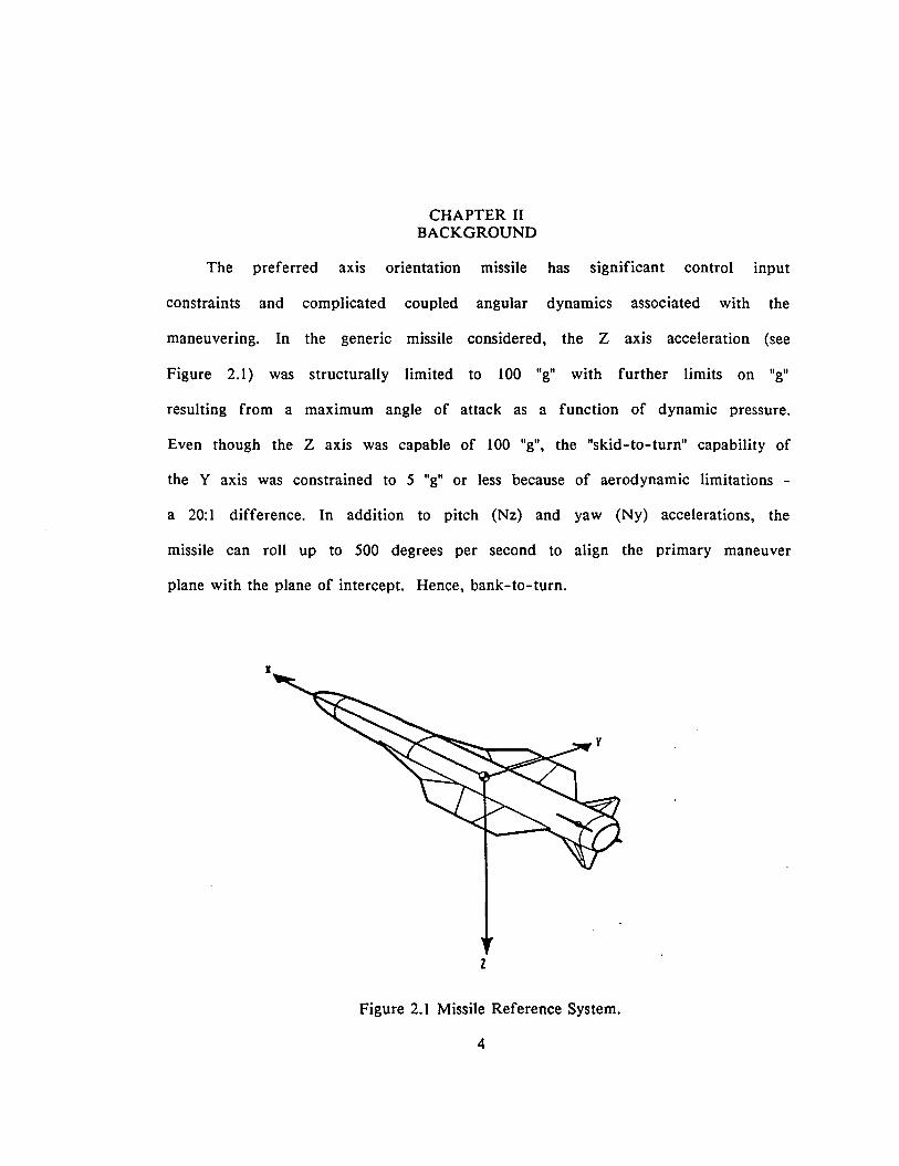
CHAPTER IIBACKGROUND
The preferred axis orientation missile has significant control input
constraints and complicated coupled angular dynamics associated with the
maneuvering. In the generic missile considered, the Z axis acceleration (see
Figure 2.1) was structurally limited to 100 "g" with further limits on "g"
resulting from a maximum angle of attack as a function of dynamic pressure.
Even though the Z axis was capable of 100 "g", the "skid-to-turn" capability of
the Y axis was constrained to 5 "g" or less because of aerodynamic limitations -
a 20:1 difference. In addition to pitch (Nz) and yaw (Ny) accelerations, the
missile can roll up to 500 degrees per second to align the primary maneuver
plane with the plane of intercept. Hence, bank-to-turn.
x
z
Figure 2.1 Missile Reference System.
4
5
The classical technique for homing missile guidance is proportional
navigation (pro nav). This technique controls the seeker gimbal angle rate to
zero which (given constant velocity) causes the missile to fly a straight line
trajectory toward the target [14,15]. In the late 70's an effort was made to use
modern control theory to improve guidance laws for air-to-air missiles. For
recent research on this problem see, for example, [11]. As stated in the
introduction, these efforts have not significantly improved the performance of
the preferred axis homing missile.
Of the modern techniques, two basic methodologies have emerged: one
was a body-axis oriented control law that used singular perturbation techniques
to uncouple the pitch & roll axis [16,17]. This technique assumed that roll rate
is the fast variable, an assumption that may not be true during the terminal
phase of an intercept. The second technique was an inertial point mass
formulation that controls inertial accelerations [18]. The acceleration commands
are fixed with respect to the missile body; but, since these commands can be
related to the inertial reference via the Euler Angles, the solution is straight
forward. Both of these methods have usually assumed unlimited control available
and the inertial technique has relied on the autopilot to control the missile roll
angle, and therefore attitude, to derotate from the inertial to body axis.
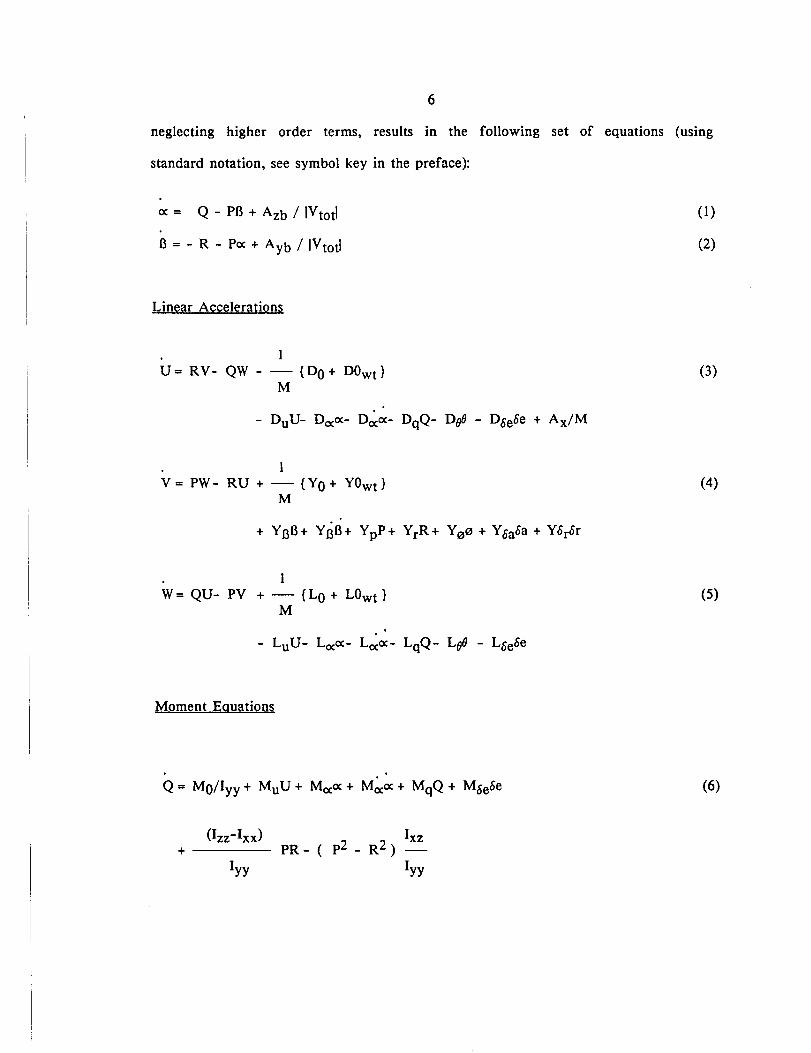
Missile Dynamics
The actual missile dynamics are a coupled set of nonlinear forces and
moments resolved along the (rotating) body axes of the missile [19].
Linearization of the equations about a "steady state" or trim condition,
6
neglecting higher order terms, results in the following set of equations (using
standard notation, see symbol key in the preface):
ex = Q - PB + Azb / IVtotl
B = - R - Pex + Ayb / IVtotl
Linear Accelerations
IU= RV- QW - - {DO+ DOwt }
M
IV = PW - RU + - {yo + YOwtl
M
+ Yf3B+ YaB+ YpP+ YrR+ Y0 0 + Yoaoa + Yoror
IW= QU- PV + - {LO + LOwt }
M
Moment Equations
Q = MO/Iyy + MuU + Mexex + Mexex + MqQ + Moeoe
(1)
(2)
(3)
(4)
(5)
(6)
+ -----I yy Iyy
7
(7)
+
(8)
+
Linear Quadratic Gaussian Control Law
For all of the modern development models, a variation of a
fixed-final-time LQG controller was used to shape the trajectory. Also, it was
expected that the autopilot would realize the commanded acceleration. First,
consider the effect of the unequal body axis constraints. Assume that 100 "g"
was commanded in each axis resulting in an acceleration vector 45 degrees from
Nz. If Ny is only capable of 5 "g", the resultant vector will be 42 degrees in
error, an error that will have to be corrected by succeeding guidance
commands. Even if the missile has the time or capability to complete a
successful intercept, the trajectory can not be considered optimal.
Now consider the nonlinear nature of the dynamics. The inertial linear
system is accurately modeled as a double integrator of the acceleration to
determine position. However, the acceleration command is a function of the
missile state, equation (1), and therefore, it is not possible to arbitrarily assign
the input acceleration. And, given a body axis linear acceleration, the inertial
8
component will be severely modified by the rotation (especially roll) of the
reference frame. All of these effects are neglected in the linearization.
This then is the problem: In the intercept trajectories worth discussing,
Ny, Nz, and roll acceleration commands will, at some time, saturate. High order,
linear approximations do not adequately model the effects of nonlinear
dynamics, and the complete two point boundary value problem with control
input dynamics and constraints is too difficult to complete in real time.
Although stochastic models are discussed in Bryson and Ho [7], and a
specific technique is introduced by Fiske [18], the general procedure has been
to use filtered estimates and a dynamic-programming-like definition of
optimality (using the Principle of Optimality) with Assumed Certainty
Equivalence to find control policies [20,21,22]. Therefore, all of the controllers
actually designed for the preferred axis missiles are deterministic laws cascaded
with a Kalman Filter. The baseline for our analysis is an advanced control law
proposed by Fiske [18]. Given the finite dimensional linear system:
where
and
x
x(t) = Fx(t) + Gu(t)
xyzVxVyVz
(9)
9
with the cost functional:
Jtf
l=xfPfxf + 1 uTRudrto
R = I
(10)
Application of the Maximum principle results in a linear optimal control law:
=-----3(Tgo)
31 +(Tgo)3+
3(Tgo)2
31 +(Tgo)3
(11 )
Coordinates used for this system are "relative inertial." The orientation of the
inertial system is established at the launch point. The distances and velocities
are the relative measures between the missile and the target. Consequently, the
set point is zero, with the reference frame moving with the missile similar to a
"moving earth" reference used in navigation.
Since Fisk's control law was based on a point mass model, the control law
did not explicitly control the roll angle PHI (0). The roll angle was controlled
by a bank-to-turn autopilot [23]. Therefore, the guidance problem was
decomposed into two components, trajectory formation and control. The
autopilot attempted to control the roll so that the preferred axis (the -Z axis)
was directed toward the plane of intercept. The autopilot used to control the
missile was designed to use proportional navigation and is a classical
combination of single loop systems.
Recently, Williams and Friedland have developed a new bank-to-turn
autopilot based on modern state space methods [24]. In order to accurately
control the banking maneuver, the missile dynamics are augmented to include
the kinematic relations describing the change in the commanded specific force
10
vector with bank angle. To determine the actual angle through which the
vehicle must roll, define the roll angle error:
Aybe", = tan- l{-- }
Azb(12)
Using the standard relations for the derivative of a vector in a rotating
reference frame, the following relationships follow from the assumption that
A 11« AlB:
Azb = - P(Ayb)
Ayb = + P(Azb)
(13)
(14)
The angle e", represents the error between the actual and desired roll angle of
the missile. Differentiating e", yields:
(Azb)(Ayb) - (Ayb)(Azb)e", =
(Azb)2 + (AYb)2
which, after substituting components of Ax w, shows that
(15)
(16)
Simplifying the nonlinear dynamics of (1) - (8), the following model was
used:
oe = Q - PJ3 + Azb / IVtotl
13 = - R - Poe + Ayb / IVtotl
(Izz - Ixx)Q = Moeoe + MqQ + MSeSe + -----
IyyPR
(17)
(18)
(19)
where
PQ (20)
(21 )
(22)
(23)
Using this model directly, the autopilot would be designed as an
eighth-order system with time-varying coefficients. However, even though these
equations contain bilinear terms involving the roll rate P as well as pitch/yaw
cross-coupling terms, the roll dynamics alone, represent a second order system
that is independent of pitch and yaw. Therefore, using an "Adiabatic
Approximation" where the optimal solution of the time-varying system is
approximated by a sequence of solutions of the time-invariant algebraic Riccati
equation for the optimum control law at each instant of time, the model was
separated into roll and pitch/yaw subsystems [25]. Now, similar to a singular
perturbations technique, the function of the roll channel is to provide the
necessary orientation of the missile so that the specific force acceleration lies
on the Z (preferred) axis of the missile. Using this approximation, the system is
assumed to be in steady state, and all coefficients--including roll rate--are
assumed to be constant. Linear Quadratic Gaussian (LQG) synthesis is used, with
an algebraic Riccati equation, on a second and sixth order system. And, when
necessary, the gains are scheduled as a function of the flight condition.
12
While still simplified, this formulation differs significantly from previous
controllers in two respects. First, the autopilot explicitly controls the roll
angle; and second, the pitch and yaw dynamics are coupled.
Even though preliminary work with this controller demonstrated improved
tracking performance by the autopilot, overall missile performance, measured by
miss distance and time to intercept, did not improve. However, the autopilot
still relies on a trajectory generated by the baseline controller ( e.g. Azb in
17). Consequently, the missile performance problem is not in the autopilot, the
error source is in the linear optimal control law which forms the trajectory.
"Reachable Set Control" is a LQG formulation that can minimize these errors.
CHAPTER IIICONSTRAINED CONTROL
In Chapters I and II, we covered the non-linear plant, the dynamics
neglected in the linearization, the impact of control variable constraints, and
the inability of improved autopilots to reduce the terminal error. To solve this
problem, we must consider the optimal control of systems subject to input
constraints. Although a search of the constrained control literature did not
provide any suitable technique for real time implementation, some of the
underlying concepts were used in the formulation of "Reachable Set Control."
This Chapter reviews some of these results to focus on the constrained control
problem and illustrate the concepts.
Much of the early work was based on research reported by Tufts and
Shnidman [26] which justified the use of saturated linear control. However, as
stated in the introduction, with saturated linear control, controllability is not
assured. If the system, boundary values and final time are such that there is no
solution with any allowable control (If the trajectory is not controllable), then
the boundary condition will not be met by either a zero terminal error or
penalty function controller. While constrained control can be studied in a clas-
sical way by searching for the effect of the constraint on the value of the
performance function, this procedure is not suitable for real time control of a
system with a wide range of initial conditions [27]. Some of the techniques that
could be implemented in real time are outlined below.
13
14
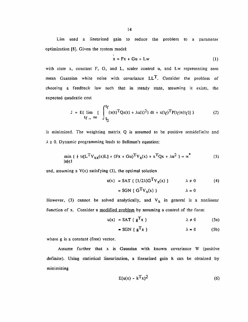
Lim used a linearized gain to reduce the problem to a parameter
optimization [8]. Given the system model:
x = Fx + Gu + Lw (1)
with state x, constant F, G, and L, scaler control u, and Lw representing zero
mean Gaussian white noise with covariance LLT. Consider the problem of
choosing a feedback law such that in steady state, assuming it exists, the
expected quadratic cost
Itf
J = E{ lim [ (x(t)TQx(t) + >.u(t)2) dt + X(tf)Tp(tf)X(tf)] }tf - 00 to
(2)
is minimized. The weighting matrix Q is assumed to be positive semidefinite and
>. ~ O. Dynamic programming leads to Bellman's equation:
min { t tr[LTYxx(x)L) + (Fx + Gu)Tyx(x) + xTQx + >.u2 } = 0:.*lul~l
and, assuming a Y(x) satisfying (3), the optimal solution
u(x) = SAT {(1/2>')GTy x(x) }
= SGN { GTyx(x) }
(3)
(4)
However, (3) cannot be solved analytically, and Yx in general is a nonlinear
function of x. Consider a modified problem by assuming a control of the form:
u(x) = SAT { gTx }
= SGN {gTx }
where g is a constant (free) vector.
>'=0
(5a)
(5b)
Assume further that x is Gaussian with known covariance W (positive
definite). Using statistical linearization, a linearized gain k can be obtained by
minimizing
E{u(x) - kTx}2 (6)
15
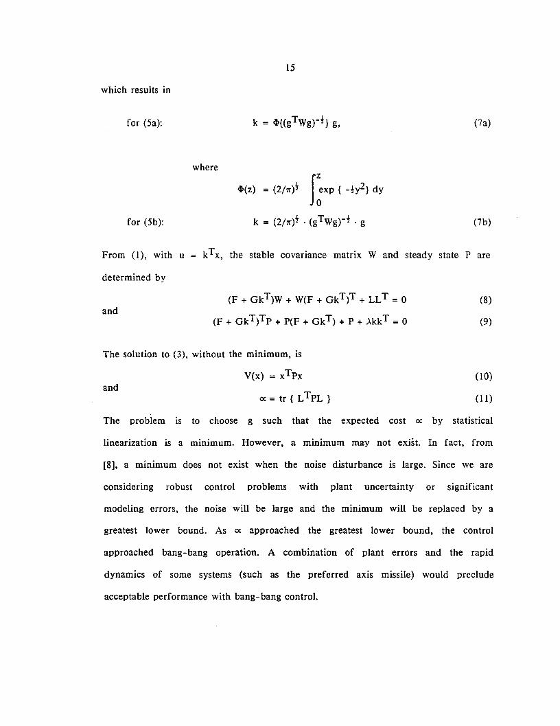
which results in
for (Sa):
for (Sb):
where
4>(z) = (2Mt J;xp ( -ty2) dy
k = (2/7l")t . (gTWg)-t . g
(7a)
(7b)
From (1), with u
determined by
kTx, the stable covariance matrix Wand steady state Pare
and(F + GkT)W + W(F + GkT)T + LLT = 0
(F + GkT)Tp + P(F + GkT) + P + >.kkT = 0
(8)
(9)
and
The solution to (3), without the minimum, is
v(x) = xTpx
ex = tr { LTPL }
(10)
(11 )
The problem is to choose g such that the expected cost ex by statistical
linearization is a minimum. However, a minimum may not exist. In fact, from
[8], a minimum does not exist when the noise disturbance is large. Since we are
considering robust control problems with plant uncertainty or significant
modeling errors, the noise will be large and the minimum will be replaced by a
greatest lower bound. As ex approached the greatest lower bound, the control
approached bang-bang operation. A combination of plant errors and the rapid
dynamics of some systems (such as the preferred axis missile) would preclude
acceptable performance with bang-bang control.
16
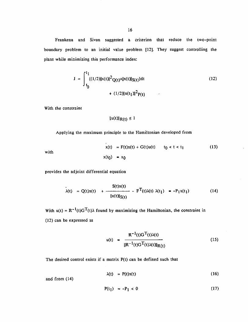
Frankena and Sivan suggested a criterion that reduce the two-point
boundary problem to an initial value problem [12]. They suggest controlling the
plant while minimizing this performance index:
With the constraint
lIu(t)IIR(t) ~ 1
Applying the maximum principle to the Hamiltonian developed from
(12)
x(t) = F(t)x(t) + G(t)u(t)with
x(to) = xO
provides the adjoint differential equation
to<t<tl (13)
).(t) = Q(t)x(t) +S(t)x(t)
II x(t)IIS(t)(14)
With u(t) = R-I(t)GT(t»). found by maximizing the Hamiltonian, the constraint in
(12) can be expressed as
R-1(t)GT(t»).(t)u(t) =
IIR-1(t)GT(t»).(t)IIR(t)
The desired control exists if a matrix P(t) can be defined such that
).(t) = P(t)x(t)and from (14)
P(tl) = -PI < 0
(15)
(16)
(17)
17
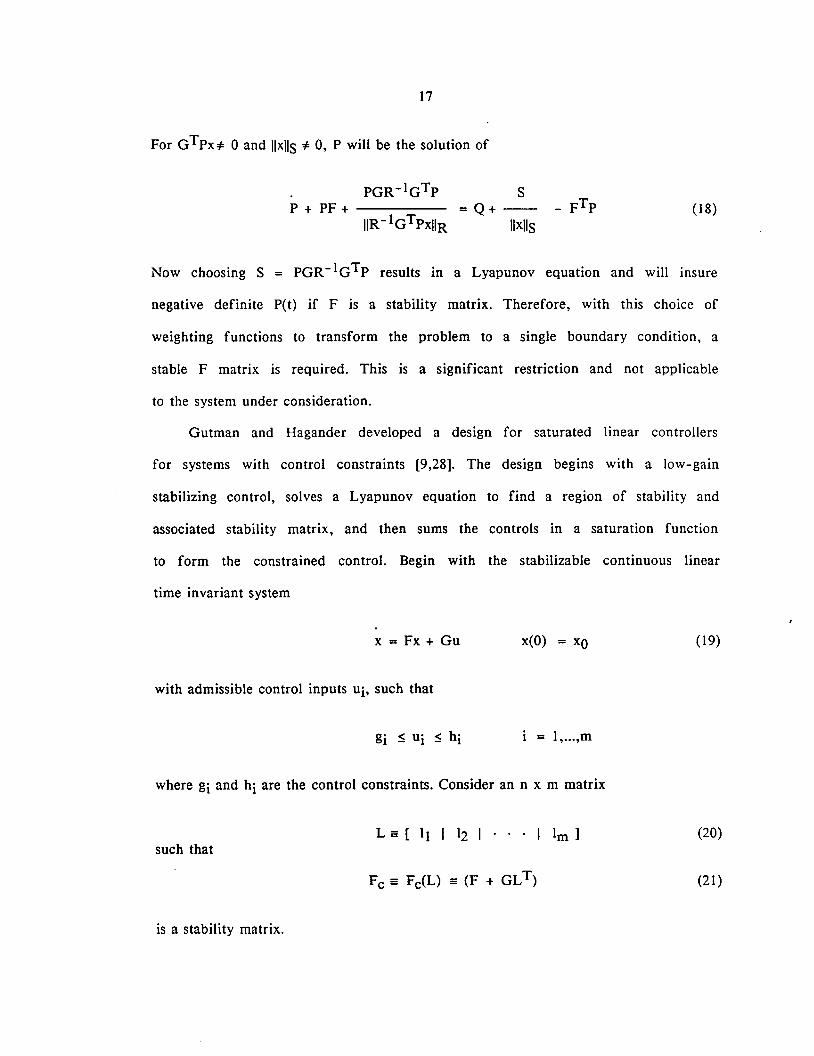
For GTPx:;: 0 and IIxliS :;: 0, P will be the solution of
PGR-IGTp SP + PF + = Q+ -- - FTP
IIR - IGTpxIlR II xliS(18)
Now choosing S = PGR-IGTp results in a Lyapunov equation and will insure
negative definite P(t) if F is a stability matrix. Therefore, with this choice of
weighting functions to transform the problem to a single boundary condition, a
stable F matrix is required. This is a significant restriction and not applicable
to the system under consideration.
Gutman and Hagander developed a design for saturated linear controllers
for systems with control constraints [9,28]. The design begins with a low-gain
stabilizing control, solves a Lyapunov equation to find a region of stability and
associated stability matrix, and then sums the controls in a saturation function
to form the constrained control. Begin with the stabilizable continuous linear
time invariant system
x = Fx + Gu
with admissible control inputs ui, such that
x(O) = xO
= l,... ,m
(19)
where gi and hi are the control constraints. Consider an n x m matrix
L == [ 11 I 12 I . . . I 1m ]such that
is a stability matrix.
(20)
(21 )
18
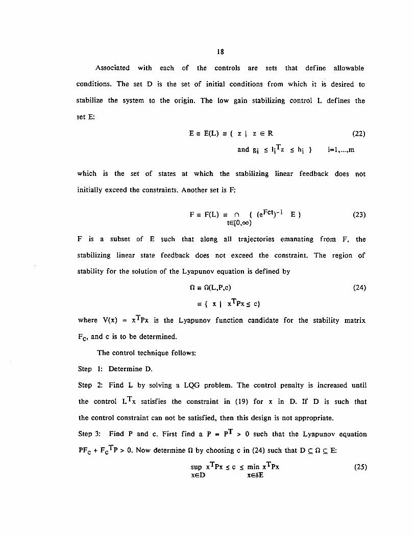
Associated with each of the controls are sets that define allowable
conditions. The set D is the set of initial conditions from which it is desired to
stabilize the system to the origin. The low gain stabilizing control L defines the
set E:
E == E(L) == ( z I z E R (22)
i=I,... ,m
which is the set of states at which the stabilizing linear feedback does not
initially exceed the constraints. Another set is F:
F == F(L) == n {(eFct)-1 E}tE[O,oo)
(23)
(24)
F is a subset of E such that along all trajectories emanating from F, the
stabilizing linear state feedback does not exceed the constraint. The region of
stability for the solution of the Lyapunov equation is defined by
0== O(L,P,c)
== { x I xTPx ~ c}
where V(x) = xTpx is the Lyapunov function candidate for the stability matrix
Fc, and c is to be determined.
The control technique follows:
Step 1: Determine D.
Step 2: Find L by solving a LQG problem. The control penalty is increased until
the control LTx satisfies the constraint in (19) for x in D. If D is such that
the control constraint can not be satisfied, then this design is not appropriate.
Step 3: Find P and c. First find a P = PT > 0 such that the Lyapunov equation
PFc + FcTp > O. Now determine 0 by choosing c in (24) such that D ~ 0 ~ E:
sup xTPx ~ c ~ min xTPxxED xE&E
(25)
19
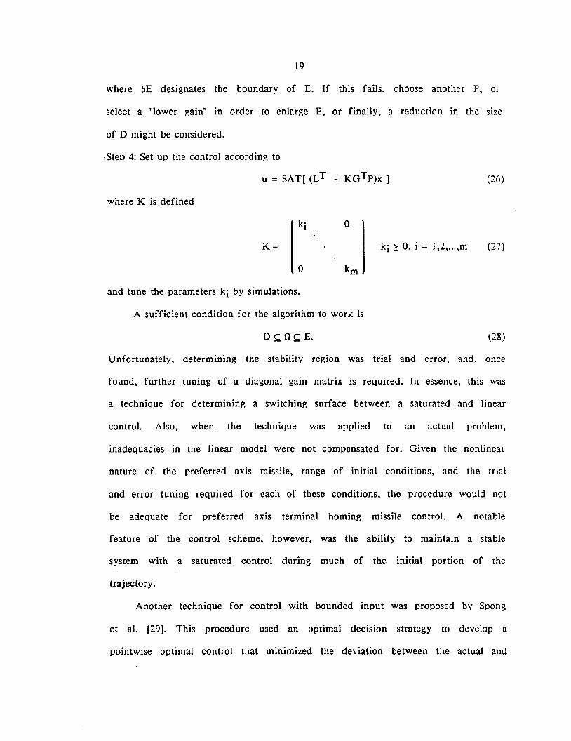
where 6E designates the boundary of E. If this fails, choose another P, or
select a "lower gain" in order to enlarge E, or finally, a reduction in the size
of D might be considered.
Step 4: Set up the control according to
u = SAT[ (LT - KGTp)x]
where K is defined
(26)
K= [k
i
0] ki ~ 0, i = 1,2,... ,m (27)
o km
and tune the parameters ki by simulations.
A sufficient condition for the algorithm to work is
D ~ O~ E. (28)
Unfortunately, determining the stability region was trial and error; and, once
found, further tuning of a diagonal gain matrix is required. In essence, this was
a technique for determining a switching surface between a saturated and linear
control. Also, when the technique was applied to an actual problem,
inadequacies in the linear model were not compensated for. Given the nonlinear
nature of the preferred axis missile, range of initial conditions, and the trial
and error tuning required for each of these conditions, the procedure would not
be adequate for preferred axis terminal homing missile control. A notable
feature of the control scheme, however, was the ability to maintain a stable
system with a saturated control during much of the initial portion of the
trajectory.
Another technique for control with bounded input was proposed by Spong
et al. [29]. This procedure used an optimal decision strategy to develop a
pointwise optimal control that minimized the deviation between the actual and
20
desired vector of joint accelerations, subject to input constraints. The
computation of the control law is reduced to the solution of a weighted
quadratic programming problem. Key to this solution is the availability of a
desired trajectory in state space. Suppose that a dynamical system can be
described by
with
which can be written as
x(t) = f(x(t» + G(x(t»u(t)
Nu~ c
(29)
Fix time t ~ 0, let s(t,xo,to,u(t» (or s(t) for short), denote the solution to (29)
corresponding to the given input function u(t). At time t, ds/dt is the velocity
vector of the system, and is given explicitly by the right hand side of (29).
Define the set Ct = C(s(t»
with
C(s(t» = ( ex(t,w) E RN I ex
= f(s(t» + G(s(t»w, w E {} }
{} = { w I NW:5 C }
(30)
Therefore, for each t and any allowable u(t), ds/dt lies in the set Ct. In other
words, the set Ct contains the allowable velocities of the solution s(t). Assume
that there exists a desired trajectory yd, and an associated vector field v(t) =
v(s(t),yd(t),t», which is the desired (state) velocity of s(t) to attain yd.
Consider the following "optimal decision strategy" for a given positive
definite matrix Q: Choose the input u(t) so that the corresponding solution s(t)
satisfies (d/dt)s(t,u(t» = s*(t), where s*(t) is chosen at each t to minimize
min {(ex - v(s(t),yd(t),t»TQ( ex - v(s(t),yd(t),t» }exECt
(31)
21
This is equivalent to the minimization
min { !UTGTQGu - (GTQ(v-f»Tu } subject to, Nu(t) ~ cu
(32)
We may now solve the quadratic programming problem to yield a pointwise
optimal control law for (29).
At each time t, the optimal decision strategy attempts to "align" the
closed loop system with the desired velocity v(t) as nearly as possible in a least
squares sense. In this way the authors retain the desirable properties of v(t)
within the constraints imposed by the control. Reachable Set Control builds on
this technique: it will determine the desired trajectory and optimally track it.
Finally, minimum-time control to the origin using a constrained
acceleration has also been solved by a transformation to a two-dimensional un-
constrained control problem [30]. By using a trigonometric transformation, the
control is defined by an angular variable, u(t) f{cos(I3),sin(I3)}, and the control
problem was modified to the control of this angle. The constrained linear
problem is converted to an unconstrained nonlinear problem that forces a
numerical solution. This approach removes the effect of the constraints at the
expense of the continuous application of the maximum control. Given the
aerodynamic performance (range and velocity) penalty of maximum control and
the impact on attainable roll rates due to reduced stability at high angle of
attack, this concept did not fit preferred axis homing missiles.
An important assumption in the previous techniques was that the
constrained system was controllable. In fact, unlike (unconstrained) linear
systems, controllability becomes a function of the set admissible controls, the
initial state, the time-to-go, and the target state. To illustrate this, some of
the relevant points from [31,32] will be presented. An admissible control is one
22
that satisfies the condition u(·) : [0,00) - 0 E Rm where 0 is the control
restraint set. The collection of all admissible controls will be denoted by M(O).
The target set X is a specified subset in Rn. A system is defined to be
O-controllable from an initial state x(tO) = xo to the target set X at T if there
exists U(·) E M(O) such that x(T,u(·),xO) E X. A system would be globally
O-controllable to X if it is O-controllable to X from every x(tO) ERn.
In order to present the necessary and sufficient conditions for
O-controllability, consider the following system:
x(t) = F(t)x(t) + G(t,u(t»
and the adjoint defined by:
~(t) = - F(t)Tz(t)
with the state transition matrix q>(t,r) and solution
x(to) = xO
Z(to) = zO
(33)
t f [0,00) (34)
(35)
The interior B and surface S of the unit ball in Rn are defined as
B ={ZO f Rn
S={zOfRn
llzoll ~ I }
IIzoll = I }
(36)
(37)
The scaler function J(.): Rn x R x Rn x Rn - R is defined by
J(xo,t,x,zo) = XOTZO + Jt max [ GT(r,w)z(r) ]dr - x(t)Tz(t)o WfO
(38)
Given the relatively mild assumptions of [32], a necessary condition for
(33) to be O-controllable to X from x(tO) is
max min J(xO,T,x,ZO) = 0XfX zOfB
while a sufficient condition is
sup min J(xO,T,x,zO) > 0XfX ZOfS
(39)
(40)
23
The principle behind the conditions arises from the definition of the
adjoint system -- Z(t). Using reciprocity, the adjoint is formed by reversing the
role of the input and output, and running the system in reverse time [33].
Consider
x(t) = F(t)x(t) + G(t)u(t)
y(t) = H(t)x(t)and:
z(t) = - F(t)Tz(t) + HT(t)~(t)
o(t) = GT(t)z(t)
Therefore
x(to) = xO
z(to) = zO
(41)
(42)
andzT(t)x(t) = zT(F(t)x(t) + G(t)u(t»
(d/dt)(zT(t)x(t» = ~T(t)x(t) + zT(t)x'(t)
= ~T(t)H(t)x(t) + zT(t)G(t)u(t)
(43)
(44)
Integrating both sides from to to tf yields the adjoint lemma:
(45)
The adjoint defined in (31) does not have an input. Consequently, the
integral in (35) is a measure of the effect of the control applied to the original
system. By searching for the maximum GT(r,w)z(r), it provides the boundary of
the effect of allowable control on the system (33). Restricting the search over
the target set to the min ( J(xo,t,x,zO) : t f [O,T], zo f S } or min (
J(xo,t,x,zo) : t f [O,T], zo f B } minimizes the effect of the specific selection
of Z() on the reachable set and insures that the search is over a function that
is jointly continuous in (t,x). Consequently, (35) compares the autonomous
growth of the system, the reachable boundary of the allowable input, and the
desired target set and time. Therefore, if J = 0, the adjoint lemma is be
24
identically satisfied at the boundary of the control constraint set (necessary);
J > 0 guarantees that a control can be found to satisfy the lemma. If the lemma
is satisfied, then the initial and final conditions are connected by an allowable
trajectory. The authors [32] go on to develop a zero terminal error steering
control for conditions where the target set is closed and
max min J(xO,T,x,zO) ~ 0x€X ZO€S
(46)
But their control technique has two shortcomings: First; it requires the
selection of z00 The initial condition zo is not specified but limited to IIz01l =
1. A particular zo must be selected to meet the prescribed conditions and the
equality in (43) for a given boundary condition, and is therefore not suitable
for real time applications. And second; the steering control searched M(O) for
the supremum of J, making the control laws bang-bang in nature, again not
suitable for homing missile control.
While a direct search of Ox is not appropriate for a preferred axis missile
steering control, a "dual" system, similar to the adjoint system used in the
formulation of the controllability function J, can be used to determine the
amount of control required to maintain controllability. Once controllability is
assured, then a cost function that penalizes the state deviation (as opposed to a
zero terminal error controller) can be used to control the system to an
arbitrarily small distance from the reference.
CHAPTER IVCONSTRAINED CONTROL
WITHUNMODELED SETPOINT AND PLANT VARIAnONS
Chapter III reviewed a number of techniques to control systems subject to
control variable constraints. While none of the techniques were judged adequate
for real time implementation of a preferred-axis homing missile controller, some
of the underlying concepts can be used to develop a technique that can
function in the presence of control constraints: (l) Use of a "dual system" that
can be used to maintain a controllable system (trajectory); (2) an "optimal
decision strategy" to minimize the deviation between the actual and desired
trajectory generated by the "dual system;" and (3) initially saturated control and
optimal (real time) selection of the switching surface to linear control with zero
terminal error.
However, in addition to, and compounding the limitations imposed by
control constraints, we must also consider the sensitivity of the control to
unmodeled disturbances and robustness under plant variations. In the stochastic
problem, there are three major sources of plant variations. First, there will be
modeling errors (linearization/reductions) that will cause the dynamics of the
system to evolve in a different or "perturbed" fashion. Second, there may be
the unmodeled uncertainty in the system state due to Gaussian assumptions. And
finally, in the fixed final time problem, there may be errors in the final time,
especially if it is a function of the uncertain state or impacted by the modeling
reductions. Since the primary objective of this research is the zero error
control of a dynamical system in fixed time, most of the more recent
25
26
optimization techniques (eg. LQG/LTR,WXl) did not apply. At this time, these
techniques seemed to be more attuned to loop shaping or robust stabilization
questions.
A fundamental proposition that forms the basis of Reachable Set Control is
that excessive terminal errors encountered when using an optimal feedback
control for an initially controllable trajectory (a controllable system that can
meet the boundary conditions with allowable control values) are caused by the
combination of control constraints and uncertainty (errors) in the target set
stemming from unmodeled plant perturbations (modeling errors) or set point
dynamics.
First, a distinction must be made between a feedback and closed-loop
controller. Feedback control is defined as a control system with real-time
measurement data fed back from the actual system but no knowledge of the
form, precision, or even the existence of future measurements. Closed-loop
control exploits the knowledge that the loop will remain closed throughout the
future interval to the final time. It adds to the information provided to a
feedback controller, anticipates that measurements will be taken in the future,
and allows prior assessment of the impact of future measurements. If Certainty
Equivalence applies, the feedback law is a closed-loop law. Under the Linear
Quadratic Gaussian (LQG) assumptions, there is nothing to be gained by
anticipating future measurements. In the mathematical optimization, external
disturbances can be rejected, and the mean value of the terminal error can be
made arbitrarily close to zero by a suitable choice of control cost.
For the following discussion, the "system" consists of a controllable plant
and an uncontrollable reference or target. The system state is the relative
difference between the plant state and reference. Since changes in the system
27
boundary condition can be caused by either a change in the reference point or
plant output perturbations similar to those discussed in Chapter II, some
definitions are necessary. The set of boundary conditions for the combined plant
and target system, allowing for unmodeled plant and reference perturbations,
will be referred to as the target set. Changes, or potential for change, in the
target set caused only by target (reference) dynamics will be referred to as
variations in the set point. The magnitude of these changes is assumed to be
bounded. Admissible plant controls are restricted to a control restraint set that
limits the input vector. Since there are bounds on the input control, the system
becomes non-linear in nature, and each trajectory must be evaluated for
controllability. Assume that the system (trajectory) is pointwise controllable
from the initial to the boundary condition.
Before characterizing the effects of plant and set point variations, we
must consider the form of the plant and it's perturbations. If we assume that
the plant is nonlinear and time-varying, there is not much that can be deduced
about the target set perturbations. However, if have a reduced order linear
model of a combined linear and nonlinear process, or a reasonable linearization
of a nonlinear model, then the plant can be considered as linear and
time-varying. For example, in the case of a Euclidean trajectory. the system
model (a double integrator) is exact and linear. Usually, neglected higher order
or nonlinear dynamics or constraints modify the accelerations and lead to
trajectory (plant) perturbations. Consequently, in this case, the plant can be
accurately represented as a Linear Time Invariant System with (possibly) time
varying perturbations.
28
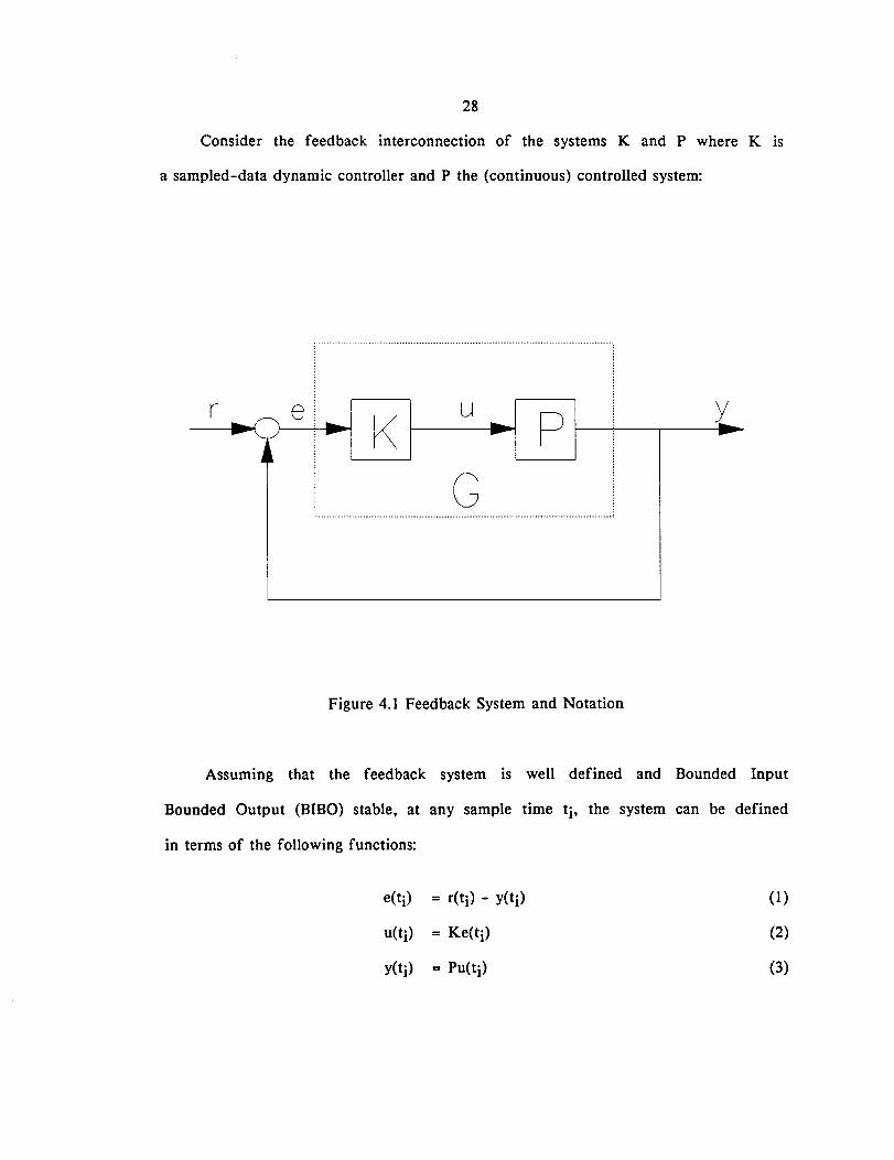
Consider the feedback interconnection of the systems K and P where K is
a sampled-data dynamic controller and P the (continuous) controlled system:
r -- Ku
G
-- p -
~ _ .:
Figure 4.1 Feedback System and Notation
Assuming that the feedback system is well defined and Bounded Input
Bounded Output (BIBO) stable, at any sample time ti, the system can be defined
in terms of the following functions:
e(ti) = r(ti) - y(ti)
u(ti) = Ke(ti)
y(ti) = Pu(ti)
(1)
(2)
(3)
with the operator G
29
G[K,P] as the operator that maps the input e(ti) to the
output y(ti) [34].
At any time, the effect of a plant perturbation DoP can also be
characterized as a perturbation in the target set.
or
then
If P = Po + DoP
P = P(I+DoP)
y(ti) = YO(tj) + Doy(ti)
(4a)
(4b)
(5)
where Doy(ti) represents the deviation from the "nominal" output caused by
either the additive or multiplicative plant perturbation. Therefore,
e(ti) = r(ti) - (YO(ti) + Doy(ti»
= (r(tj) + Doy(ti» - YO(ti)
= Dor(ti) - YO(ti)
(6)
(7)
(8)
with Dor(ti) representing a change in the target set that was unknown to the
controller. These changes are then fed back to the controller but could be
handled a priori in a closed loop controller design as target set uncertainty.
Now consider the effect of constraints. If the control is not constrained,
and target set errors are generated by plant variations or target maneuvers, the
feedback controller can recover from these intermediate target set errors by
using large (impulsive) terminal controls. The modeled problem remains linear.
While the trajectory is not the optimal closed-loop trajectory, the trajectory is
optimal based on the model and information set available.
Even with unmodeled control variable constraints, and a significant dis
placement of the initial condition, an exact plant model allows the linear
stochastic optimal controller to generate an optimal trajectory. The switching
time from saturated to linear control is properly (automatically) determined and,
30
as in the linear case, the resulting linear control will drive the state to within
an arbitrarily small distance from the estimate of the boundary condition.
If the control constraint set covers the range of inputs required by the
control law, the law will always be able to accommodate target set errors in
the remaining time-to-go. This is, in effect, the unconstrained case. If,
however, the cost-to-go is higher and/or the deviation from the boundary
condition is of sufficient magnitude relative to the time remaining to require
inputs outside the boundary of the control constraint set, the system will not
follow the trajectory assumed by the system model. If this is the case as
time-to-go approaches zero, the boundary condition will not be met, the system
is not controllable (to the boundary condition). As time-to-go decreases, the
effects of the constraints become more important.
With control input constraints, and intermediate target set errors caused
by unmodeled target maneuvers or plant variations, it may not be possible for
the linear control law to recover from the midcourse errors by relying on large
terminal control. In this case, an optimal trajectory is not generated by the
feedback controller, and, at the final time, the system is left with large
terminal errors.
Consequently, if external disturbances are adequately modeled, terminal
errors that are orders of magnitude larger than predicted by the open loop
optimal control are caused by the combination of control constraints and target
set uncertainty.
31
Linear Optimal Control with Uncertainty and Constraints
An optimal solution must meet the boundary conditions. To accomplish
this, plant perturbations and constraints must be considered a priori. They
should be included as a priori information in the system model, they must be
physically realizable, and they must be deterministic functions of a priori
information, past controls, current measurements, and the accuracy of future
measurements.
From the control point of view, we have seen that the effect of plant
parameter errors and set point dynamics can be grouped as target set
uncertainty. This uncertainty can cause a terminally increasing acceleration
profile even when an optimal feedback control calls for a decreasing input (see
Chapter 5). With the increasing acceleration caused by midcourse target set
uncertainty, the most significant terminal limitation becomes the control input
constraints. (These constraints not only affect controllability, they also limit
how quickly the system can recover from errors.) If the initial control is
saturated while the terminal portion linear, the control is still optimal. If the
final control is going to be saturated, however, the controller must account for
this saturation.
The controller could anticipate the saturation and correct the linear
portion of the trajectory to meet the final boundary condition. This control,
however, requires a closed form solution for x(t), carries an increased cost for
an unrealized constraint, and is known to be valid for monotonic ( single
switching time) trajectories only [11].
Another technique available is LQG synthesis. However, LQG assumes
controllability in minimizing a quadratic cost to balance the control error and
32
input magnitudes. As we have seen, the effects of plant parameter and
reference variations, combined with control variable constraints, can adversely
impact controllability. The challenge of LQG is the proper formulation of the
problem to function with control variable constraints while compensating for
unmodeled set point and plant variations. Reachable Set Control uses LQG
synthesis and overcomes the limitations of an anticipative control to insure a
controllable trajectory.
Control Technique
Reachable Set Control can be thought of as a fundamentally different
robust control technique based on the concepts outlined above. The usual
discussion of robust feedback control (stabilization) centers on the development
of controllers that function even in the presence of plant variations. Using
either a frequency domain or state space approach, and modeling the uncertain
ty, bounds on the allowable plant or perturbations are developed that guarantee
stability [35]. These bounds are determined for the specific plant under
consideration and a controller is designed so that expected plant variations are
contained within the stability bounds. Building on ideas presented above,
however, this same problem can be approached in an entirely different way.
This new approach begins with the same assumptions as standard techniques,
specifically a controllable system and trajectory. But, with Reachable Set
Control, we will not attempt to model the plant or parameter uncertainty, nor
the set point variation. We will, instead, reformulate the problem so that the
system remains controllable, and thus stable, throughout the trajectory even in
the presence of plant perturbations and severe control input constraints.
33
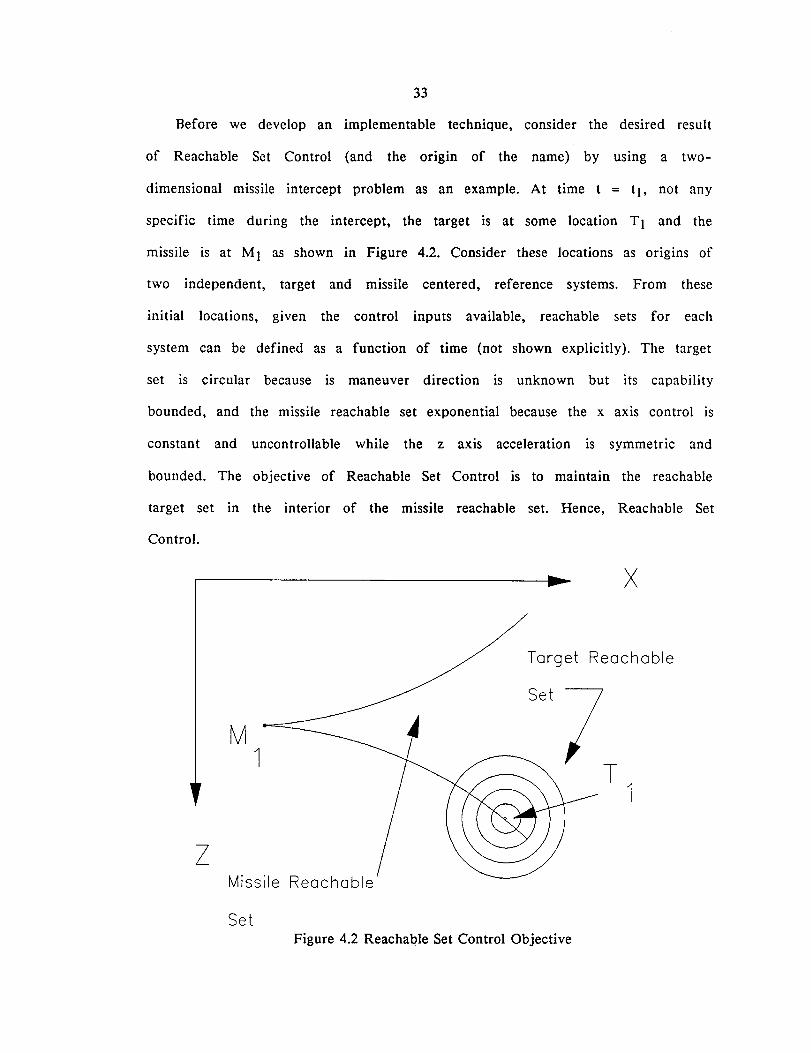
Before we develop an implementable technique, consider the desired result
of Reachable Set Control (and the origin of the name) by using a two-
dimensional missile intercept problem as an example. At time t = t}. not any
specific time during the intercept, the target is at some location T 1 and the
missile is at M I as shown in Figure 4.2. Consider these locations as origins of
two independent, target and missile centered, reference systems. From these
initial locations, given the control inputs available, reachable sets for each
system can be defined as a function of time (not shown explicitly). The target
set is circular because is maneuver direction is unknown but its capability
bounded, and the missile reachable set exponential because the x axis control is
constant and uncontrollable while the z axis acceleration is symmetric and
bounded. The objective of Reachable Set Control is to maintain the reachable
target set in the interior of the missile reachable set. Hence, Reachable Set
Control.
x
Target Reachable
M1
zMissile Reachable
SetFigure 4.2 Reachable Set Control Objective
34
As stated, Reachable Set Control would be difficult to implement as a
control strategy. Fortunately, however, further analysis leads to a simple,
direct, and optimal technique that is void of complicated algorithms or ad-hoc
procedures.
First, consider the process. The problem addressed is the control of fixed
-terminal-time systems. The true cost is the displacement of the state at the
final time and only at the final time. In the terminal homing missile problem,
this is the closest approach, or miss distance. In another problem, it may be
fuel remaining at the final time, or possibly a combination of the two. In
essence, with respect to the direct application of this technique, there is no
preference for one trajectory over another or no intermediate cost based on the
displacement of the state from the boundary condition. The term "direct
application" was used because constrained path trajectories, such as those
required by robotics, or the infinite horizon problem, like the control of the
depth of a submarine can be addressed by separating the problem into several
distinct intervals--each with a fixed terminal time--or a switching surface when
the initial objective is met [36].
Given a plant with dynamics
x(t) = f(x,t) + g(u(w),t)
y(t) = h(x(t),t)
modeled by
x(t) = F(t)x(t) + G(t)u(t)
yx(t) = H(t)x(t)
x(to) = xo (9)
(10)
35
with final condition x(tf) and a compact control restraint set Ox. Let Ox denote
the set of controls u(t) for which u(t) E Ox for t E [0,00). The reachable set
X(tO,tf,xO'Ox) == ( x: x(tf) = solution to (10)with xo for some u(·) E M(Ox) }
is the set of all states reachable from xo in time tf.
In addition to the plant and model in (9 & 10), we define the reference
(11)
r(t) = a(x,t) + b(a(w),t)
y(t) = c(x(t),t)
modeled by
r(t) = A(t)r(t) + B(t)a(t)
Yr(t) = C(t)r(t)
and similarly defined set R(to,tf,ro,Or),
r(to) = rO (12)
(13)
R(to,tf,ro,Or) == ( r: r(tf) = solution to (13)with rO for some a(·) E M(Or) }
as the set of all reference states reachable from rO in time tf.
(14)
Associated with the plant and reference, at every time t, is the following
system:
e(t) = yx(t) - Yr(t) (15)
;;m (10 & 13), we see that yx(t) and Yr(t) are output functions that
incorporate the significant characteristics of the plant and reference that will
be controlled.
The design objective is
e(tf) = 0 (16)
and we want to maximize the probability of success and minimize the effect of
errors generated by the deviation of the reference and plant from their
associated models. To accomplish this with a sampled-data feedback control law,
36
we will select the control u(ti) such that, at the next sample time (ti+l), the
target reachable set will be covered by the plant reachable set and, in steady
state, if e(tf) = 0, the control will not change.
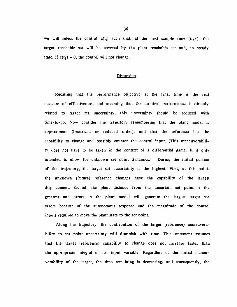
Discussion
Recalling that the performance objective at the final time is the real
measure of effectiveness, and assuming that the terminal performance is directly
related to target set uncertainty, this uncertainty should be reduced with
time-to-go. Now consider the trajectory remembering that the plant model is
approximate (linearized or reduced order), and that the reference has the
capability to change and possibly counter the control input. (This maneuverabili
ty does not have to be taken in the context of a differential game. It is only
intended to allow for unknown set point dynamics.) During the initial portion
of the trajectory, the target set uncertainty is the highest. First, at this point,
the unknown (future) reference changes have the capability of the largest
displacement. Second, the plant distance from the uncertain set point is the
greatest and errors in the plant model will generate the largest target set
errors because of the autonomous response and the magnitude of the control
inputs required to move the plant state to the set point.
Along the trajectory, the contribution of the target (reference) maneuvera
bility to set point uncertainty will diminish with time. This statement assumes
that the target (reference) capability to change does not increase faster than
the appropriate integral of its' input variable. Regardless of the initial maneu
verability of the target, the time remaining is decreasing, and consequently, the
37
ability to move the set point decreases. Target motion is smaller and it's
position is more and more certain.
Selection of the control inputs in the initial stages of the trajectory that
will result in a steady state control (that contains the target reachable set
within the plant reachable set) reduces target set uncertainty by establishing
the plant operating point and defining the effective plant transfer function.
At this point, we do not have a control procedure, only the motivation to
keep the target set within the reachable set of the plant along with a desire to
attain steady state performance during the initial stages of the trajectory. The
specific objectives are to minimize target set uncertainty, and most importantly,
to maintain a controllable trajectory. The overall objective is better
performance in terms of terminal errors.
Procedure
A workable control law that meets the objectives can be deduced from
Figure 4.3. Here we have the same reachable set for the uncertain target, but
this time, several missile origins are placed at the extremes of target motion.
From these origins, the system is run backward from the final time to the
current time using control values from the boundary of the control constraint
set to provide a unique set of states that are controllable to the specific origin.
If the intersection of these sets is non-empty, any potential target location is
reachable from this intersection. Figure 4.4 is similar, but this time the missile
control restraint set is not symmetric. Figure 4.4 shows a case where the
missile acceleration control is constrained to the set
A = [Amin,Amax] where 0 ~ Amin~ Amax (17)
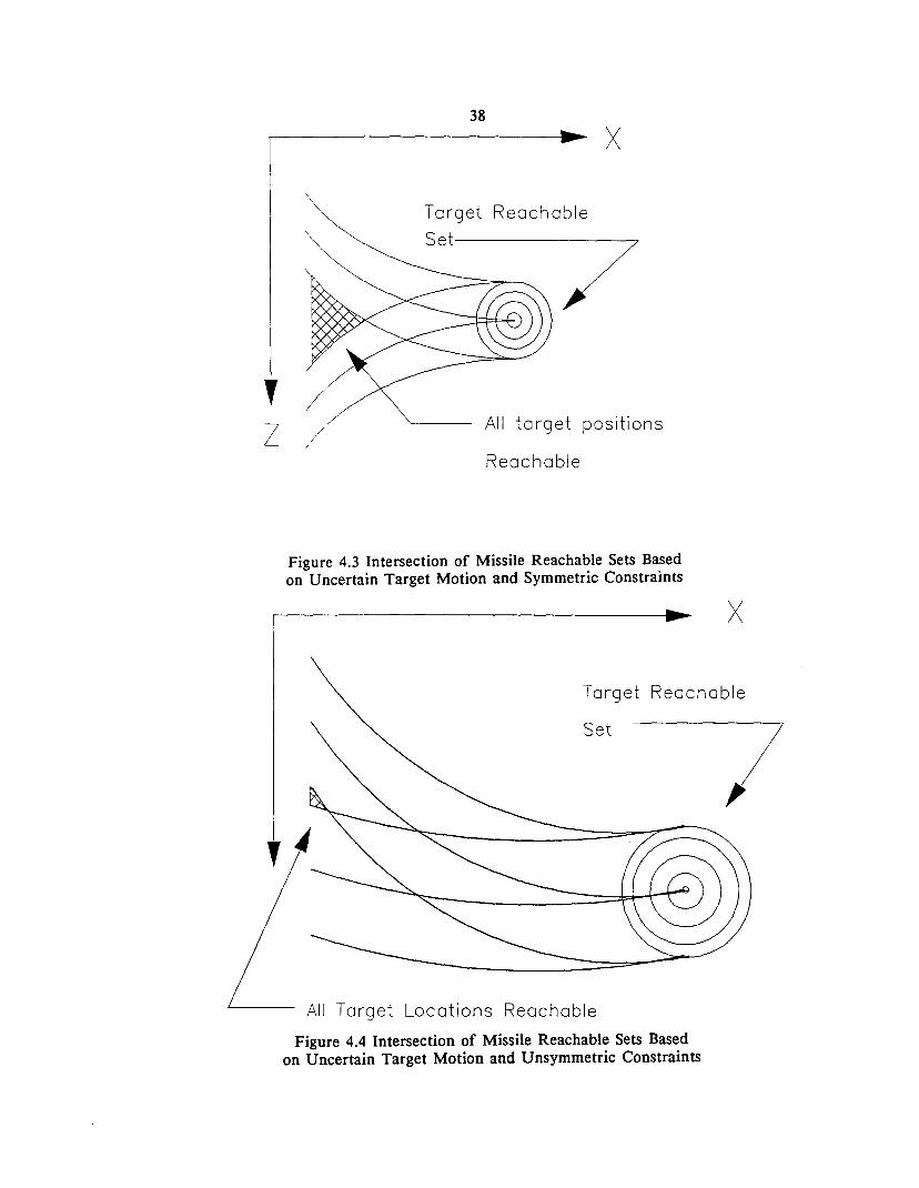
z
38
x
Target ReachableSet-------~
~~7
All target positions
Reachable
Figure 4.3 Intersection of Missile Reachable Sets Basedon Uncertain Target Motion and Symmetric Constraints
x
Target Reachable
Set
All Target Locations Reachable
Figure 4.4 Intersection of Missile Reachable Sets Basedon Uncertain Target Motion and Unsymmetric Constraints
39
Since controllability is assumed, which for constrained control includes the
control bounds and the time interval, the extreme left and right (near and far)
points of the set point are included in the set drawn from the origin.
To implement the technique, construct a dual system that incorporates
functional constraints, uncontrollable modes, and uses a suitable control value
from the control constraint set as the input. From the highest probability target
position at the final time, run the dual system backward in time from the final
boundary condition. Regulate the plant (system) to the trajectory defined by
the dual system. In this way, the fixed-final-time zero terminal error control is
accomplished by re-formulating the problem as optimal regulation to the dual
trajectory.
In general, potential structures of the constraint set preclude a specific
point (origin, center, etc.) from always being the proper input to the dual
system.
Regulation to a "dual" trajectory from the current target position will
insure that the origin of the target reachable set remains within the reachable
set of the plant. Selection of a suitable interior point from the control restraint
set as input to the dual system will insure that the plant has sufficient control
power to prevent the target reachable set from escaping from the interior of
the plant reachable set.
Based on unmodeled set point uncertainty, symmetric control constraints,
and a double integrator for the plant, a locus exists that will keep the target
in the center of the missile reachable set. If the set point is not changed, this
trajectory can be maintained without additional inputs. For a symmetric control
restraint set, especially as the time-to-go approaches zero, Reachable Set
Control is control to a "coasting" (null control) trajectory.
40
If the control constraints are not symmetric, such as Figure 4.4, a locus of
points that maintains the target in the center of the reachable set is the
trajectory based on the system run backward from the final time target location
with the acceleration command equal to the midpoint of the set A. Pictured in
Figures 4.2 to 4.4 were trajectories that are representative of the double
integrator. Other plant models would have different trajectories.
Reachable Set Control is a simple technique for minimizing the effects of
target set uncertainty and improving terminal the performance of a large class
of systems. We can minimize the effects of modeling errors (or target set un
certainty) by a linear optimal regulator that controls the system to a steady
state control. Given the well known and desirable characteristics of LQG
synthesis, this technique can be used as the basis for control to the desired
"steady state control" trajectory. The technique handles constraints by insuring
an initially constrained trajectory. Also, since the large scale dynamics are
controlled by the "dual" reference trajectory, the tracking problem be optimized
to the response time of the system under consideration. This results in an
"adaptable" controller because gains are based on plant dynamics and cost while
the overall system is smoothly driven from some large displacement to a region
where the relatively high gain LQG controller will remain linear.
CHAPTER VREACHABLE SET CONTROL EXAMPLE
Performance Comparison - Reachable Set and LOG Control
In order to demonstrate the performance of "Reachable Set Control" we
will contrast its performance with the performance of a linear optimal
controller when there is target set uncertainty combined with input constraints.
Consider, for example, the finite dimensional linear system:
with the quadratic cost
x(to) = xo (1)
where
J1
= - XfTpfXf2
(2)
and
tf E [0,00)
'1 ~ 0
Application of maximum principle yields the following linear optimal control
law:
where
1u = + - x(tf)(t-tf)
'1
xo + xo • tfx(tf) =
1 +
41
(3)
(4)
42
Appropriately defining t, to, and tf, the control law can be equivalently
expressed in an open loop or feedback form with the latter incorporating the
usual disturbance rejection properties. The optimal control will tradeoff the cost
of the integrated square input with the final error penalty. Consequently, even
in the absence of constraints, the terminal performance of the control is a
function of the initial displacement, time allowed to drive the state to zero, and
the weighting factor ,. To illustrate this, Figure 5.1 presents the terminal
states (miss distance and velocity) of the linear optimal controller. This plot is
a composite of trajectories with different run times ranging from 0 to 3.0
seconds. The figure presents the values of position and velocity at the final
time t = tf that result from an initial position of 1000 feet and with velocity of
1000 feet/sec with , = 10-4. Figure 5.2 depicts, as a function of the run time,
the initial acceleration (at t = 0.) associated with each of the trajectories
shown in Figure 5.1. From these two plots, the impact of short run times is
evident: the miss distance will be higher, and the initial acceleration command
will be greater. Since future set point (target) motion is unknown, the
suboptimal feedback controller is reset at each sample time to accommodate this
motion. The word reset is significant. The optimal control is a function of the
initial condition at time t = to, time, and the final time. A feedback realization
becomes a function of the initial condition and time to go only. In this case,
set point motion (target set uncertainty) can place the controller in a position
where the time-to-go is small but the state deviation is large.
Velocity2000
o-2000
-4000
-6000
-8000
-10000
-12000
-14000 o 200
43
400 600 800Position
1000 1200
Figure 5.1 Terminal Performance of Linear Optimal Control
Accelerationo
-100000 -
-200000
-300000
v-400000
o 0.5 1
Final Time1.5 2
Figure 5.2 Initial Acceleration of Linear Optimal Control
44
While short control times will result in poorer performance and higher
accelerations, it does not take a long run time to drive the terminal error to
near zero. Also, from (4) we see that the terminal error can be driven to an
arbitrarily small value by selection of the control weighting. Figure 5.1
presented the final values of trajectories running from 0 to 3 seconds. Figures
5.3 through 5.5 are plots of the trajectory parameters for the two second
trajectory (with the same initial conditions) along with the zero control
trajectory values. These values are determined by starting at the boundary
conditions of the optimal control trajectory and running the system backward
with zero acceleration. For example, if we start at the final velocity and run
backwards in time along the optimal trajectory, for each point in time, there is
a velocity (the null control velocity) that will take the corresponding position
of the optimal control trajectory to the boundary without additional input. The
null control position begins at the origin at the final time, and moving
backward in time, is the position that will take the system to the boundary
condition at the current velocity. Therefore, these are the positions and
velocities (respectively) that will result in the boundary condition without
additional input. As t => tf the optimal trajectory acceleration approaches zero.
Therefore, the zero control trajectory converges to the linear optimal
trajectory. If the system has a symmetric control constraint set, Reachable Set
Control will control the system position to the zero control (constant velocity)
trajectory.
Acceleration
o
-500
-1000
-1500
-2000
-2500 00.5
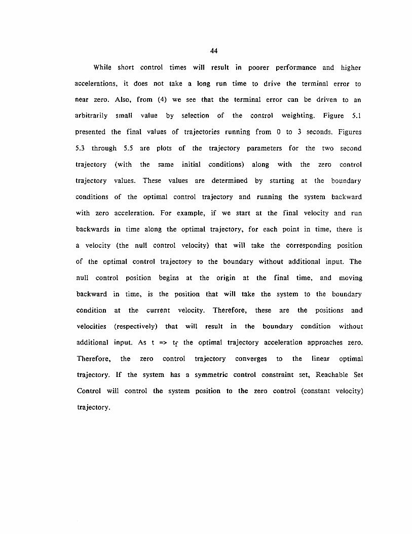
45
1Time
1.5 2
Figure 5.3 Linear Optimal Acceleration vs Time
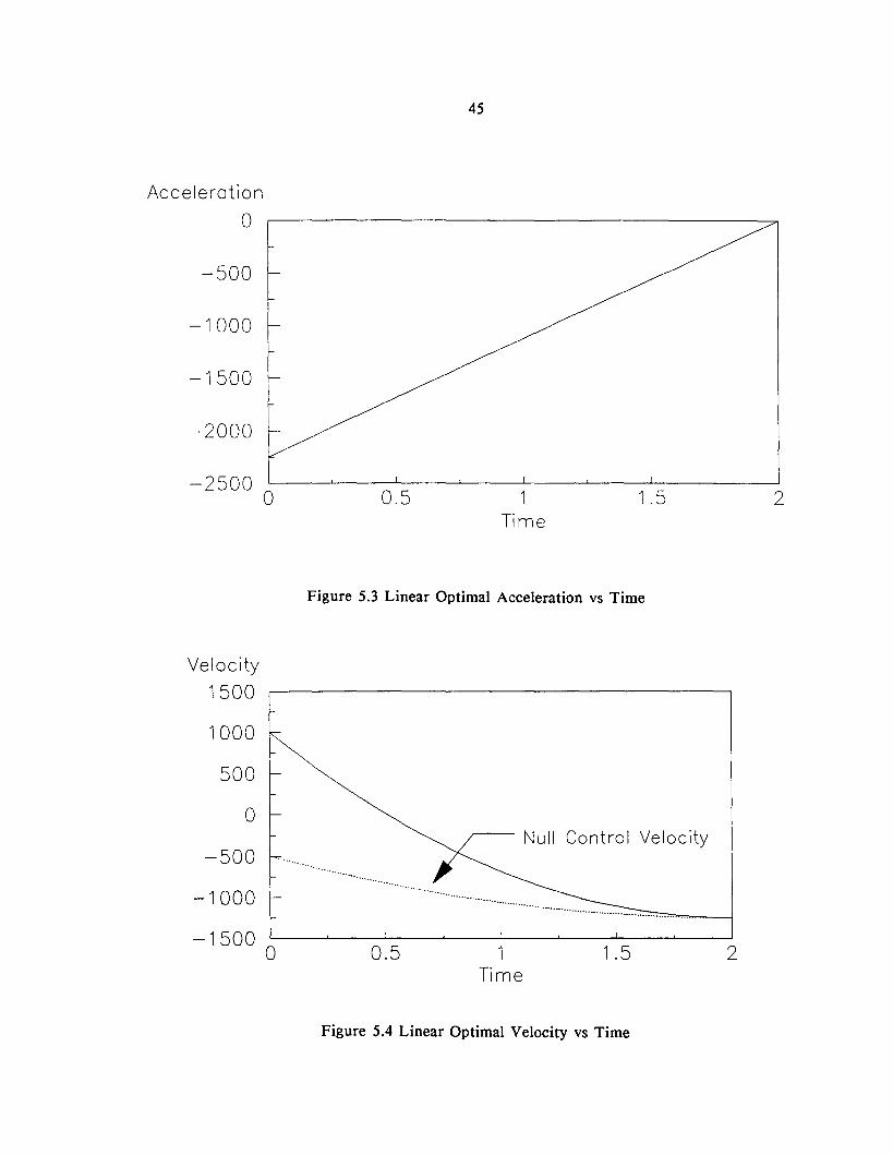
r--- Null Control Velocity
Velocity
1500
1000
500
0
-500 ........
-1000
-15000.50
..............
1Time
1.5 2
Figure 5.4 Linear Optimal Velocity vs Time
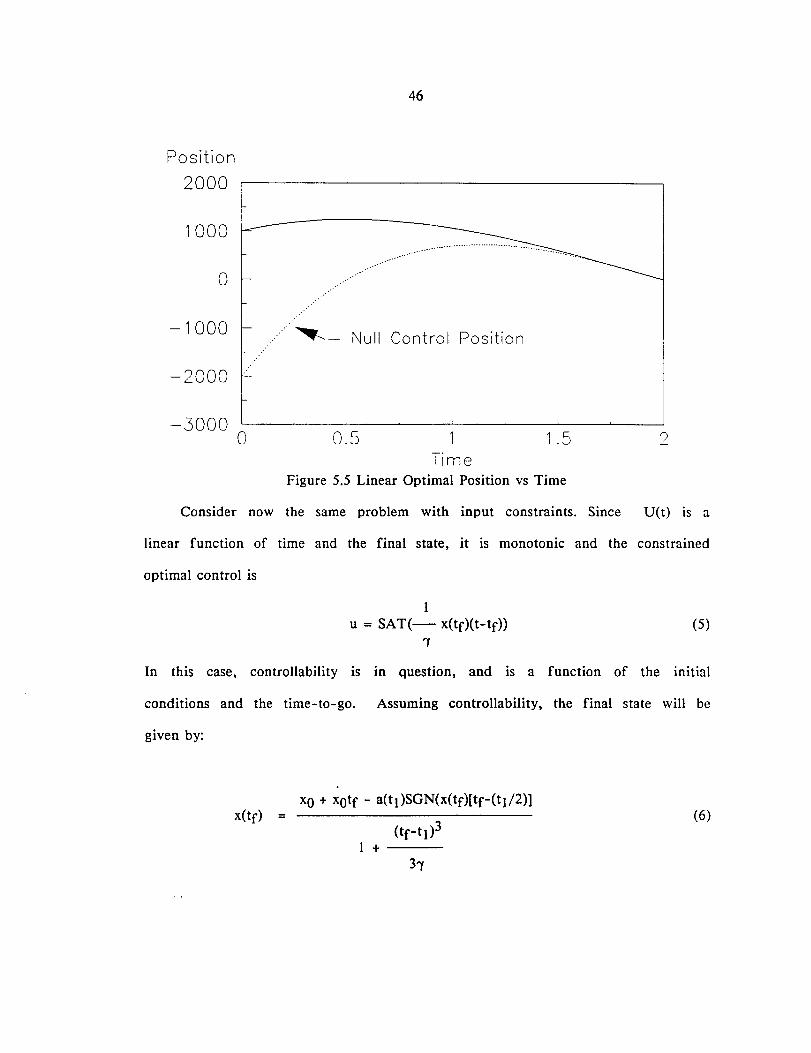
46
Position
2000
1000......
o
-1000
-2000
-3000 o
~- Null Control Position
0.5 1 1.5Time
Figure 5.5 Linear Optimal Position vs Time
2
Consider now the same problem with input constraints. Since Vet) is a
linear function of time and the final state, it is monotonic and the constrained
optimal control is
Iu = SAT(- x(tf)(t-tf» (5)
"I
In this case, controllability is in question, and is a function of the initial
conditions and the time-to-go. Assuming controllability, the final state will be
given by:
x(tf) =xQ + xQtf - a(tl)SGN(x(tf)[tf-(tl/2)]
(tf-t1)31+---
(6)
47
where tl is the switching time from saturated to linear control. The open loop
switch time can be shown to be
(7)
or the closed loop control can be used directly. In either case, the optimal
control will correctly control the system to a final state X(tf) near zero.
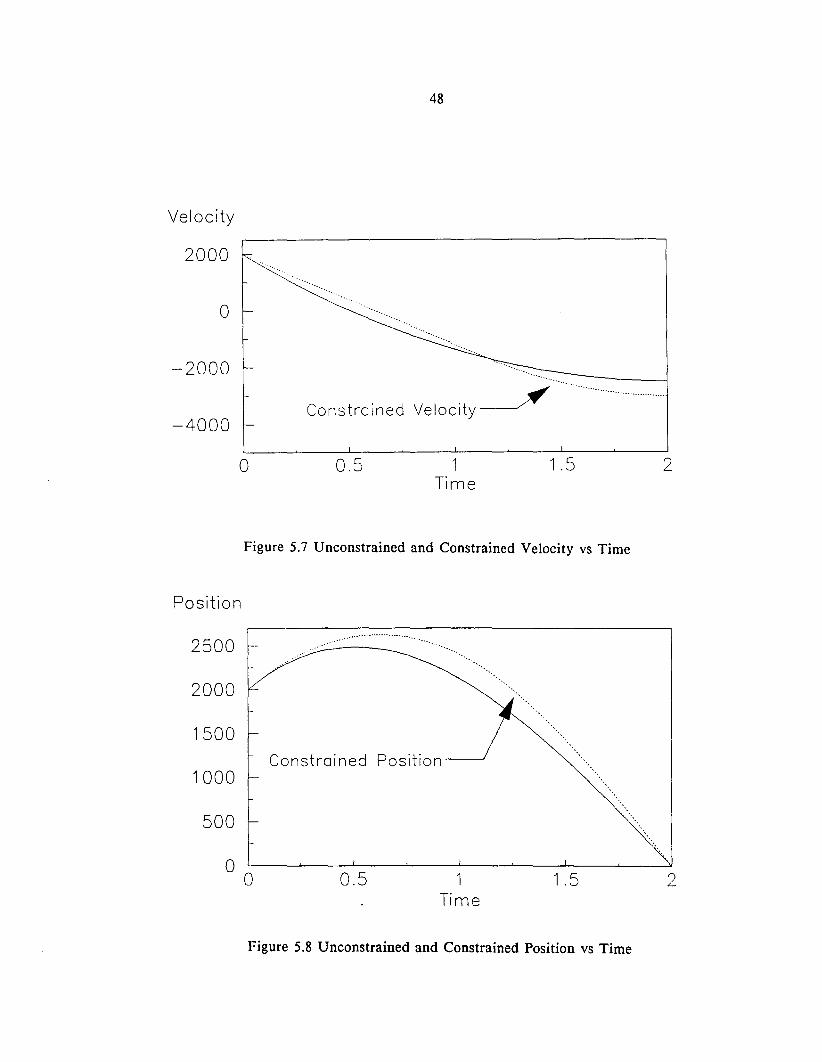
Figures 5.6 through 5.8 illustrate the impact of the constraint on the closed
loop optimal control. In each plot, the optimal constrained and unconstrained
trajectory is shown.
Acceleration
1000
o
-1000
-2000
-3000
-4000
....
.........
-5000 0 0.5 1Time
1.5 2
Figure 5.6 Unconstrained and Constrained Acceleration
48
Velocity
2000
o
-2000
-4000Constrained velocity~
o 0.5 1Time
1.5 2
Figure 5.7 Unconstrained and Constrained Velocity vs Time
......~--- .....
......
21.51Time
0.5
Constrained Position------l
Position
2500
2000
1500
1000
500
00
Figure 5.8 Unconstrained and Constrained Position vs Time
49
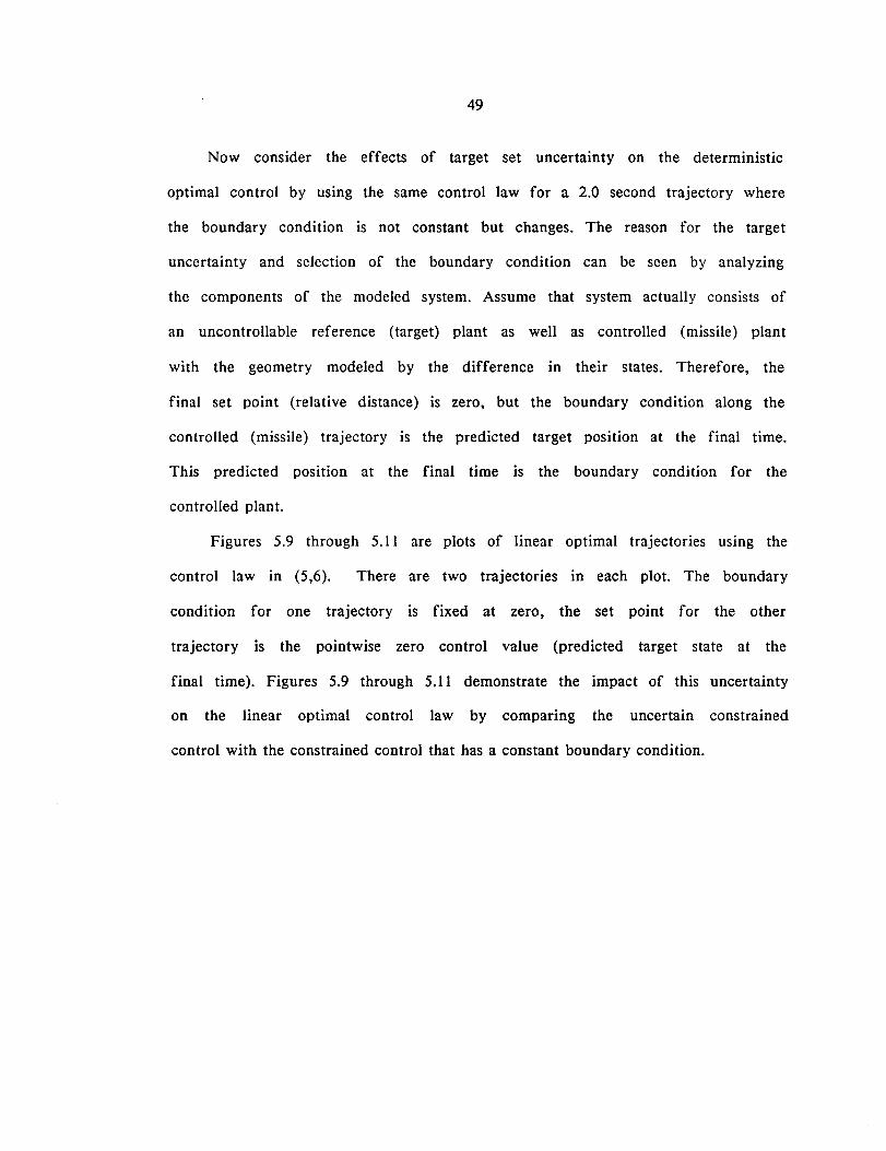
Now consider the effects of target set uncertainty on the deterministic
optimal control by using the same control law for a 2.0 second trajectory where
the boundary condition is not constant but changes. The reason for the target
uncertainty and selection of the boundary condition can be seen by analyzing
the components of the modeled system. Assume that system actually consists of
an uncontrollable reference (target) plant as well as controlled (missile) plant
with the geometry modeled by the difference in their states. Therefore, the
final set point (relative distance) is zero, but the boundary condition along the
controlled (missile) trajectory is the predicted target position at the final time.
This predicted position at the final time is the boundary condition for the
controlled plant.
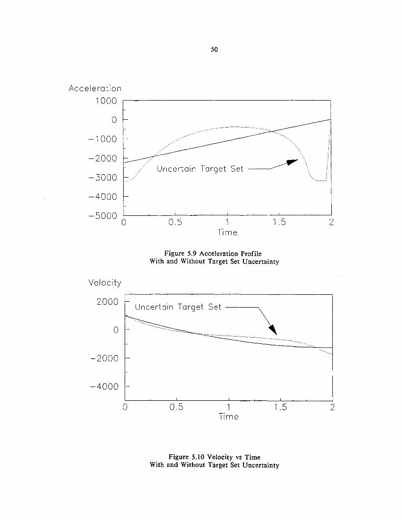
Figures 5.9 through 5.11 are plots of linear optimal trajectories using the
control law in (5,6). There are two trajectories in each plot. The boundary
condition for one trajectory is fixed at zero, the set point for the other
trajectory is the pointwise zero control value (predicted target state at the
final time). Figures 5.9 through 5.11 demonstrate the impact of this uncertainty
on the linear optimal control law by comparing the uncertain constrained
control with the constrained control that has a constant boundary condition.
Acceleration
1000
o
-1000
-2000
-3000
-4000
50
......
Uncertain Target Set~
-5000 0 0.5 1Time
1.5 2
Velocity
2000
o
-2000
-4000
Figure 5.9 Acceleration ProfileWith and Without Target Set Uncertainty
un~~r:ain Target Set \
.......................
o 0.5 1Time
1.5 2
Figure 5.10 Velocity vs TimeWith and Without Target Set Uncertainty
51
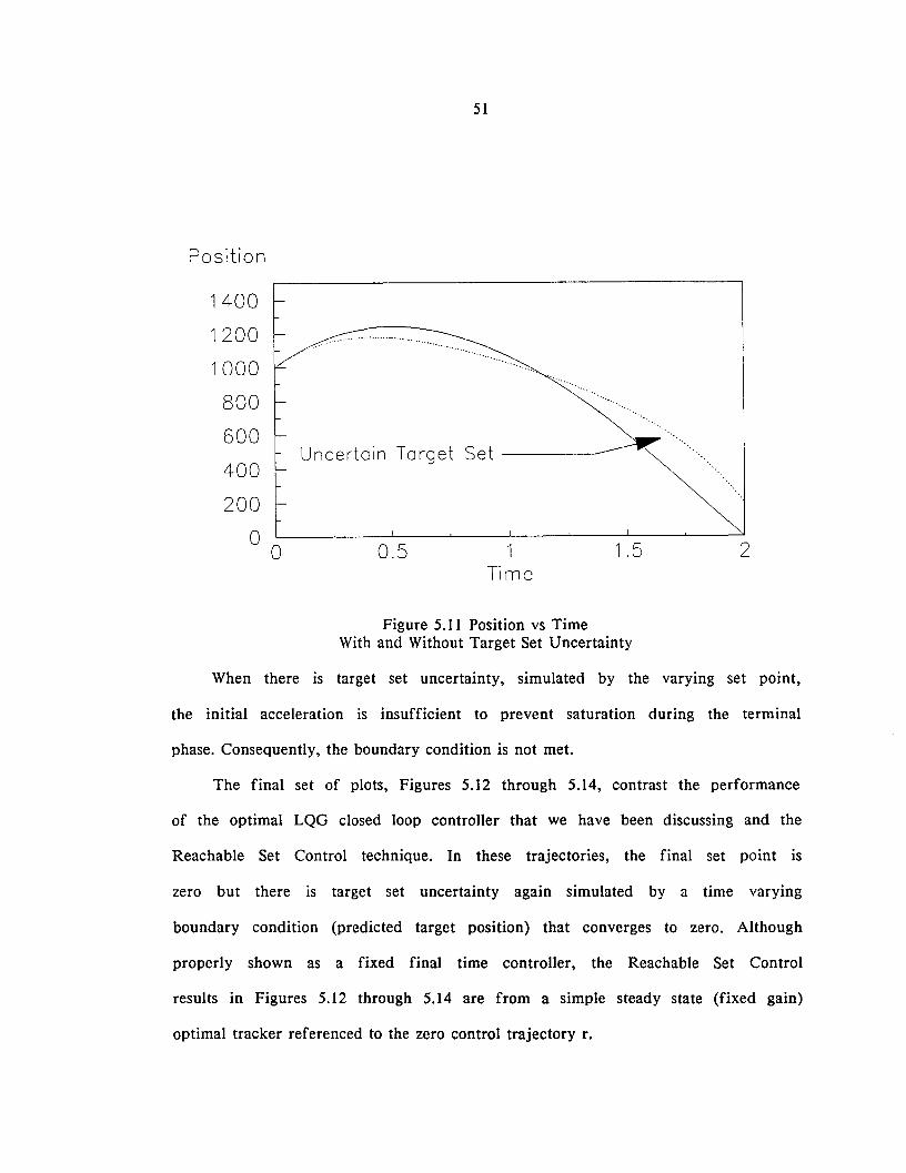
Position
Uncertain Target Set ----------
1400
1200
1000
800
600
400
200
o 0 0.5 1Time
1.5 2
Figure 5.11 Position vs TimeWith and Without Target Set Uncertainty
When there is target set uncertainty, simulated by the varying set point,
the initial acceleration is insufficient to prevent saturation during the terminal
phase. Consequently, the boundary condition is not met.
The final set of plots, Figures 5.12 through 5.14, contrast the performance
of the optimal LQG closed loop controller that we have been discussing and the
Reachable Set Control technique. In these trajectories, the final set point is
zero but there is target set uncertainty again simulated by a time varying
boundary condition (predicted target position) that converges to zero. Although
properly shown as a fixed final time controller, the Reachable Set Control
results in Figures 5.12 through 5.14 are from a simple steady state (fixed gain)
optimal tracker referenced to the zero control trajectory r.
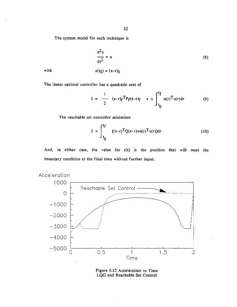
52
The system model for each technique is
(8)
with x(to) = (x-r)o
The linear optimal controller has a quadratic cost of
J =2
The reachable set controller minimizes
(9)
J = J:1) [(x-r)TQ(x-r)+u(r)Tu(r)]dr (10)
And, in either case, the value for r(t) is the position that will meet the
boundary condition at the final time without further input.
Acceleration
1000
o
-1000
-2000
-3000
-4000
Reachable Set Control~
-5000 00.5 1
Time1.5 2
Figure 5.12 Acceleration vs TimeLQG and Reachable Set Control
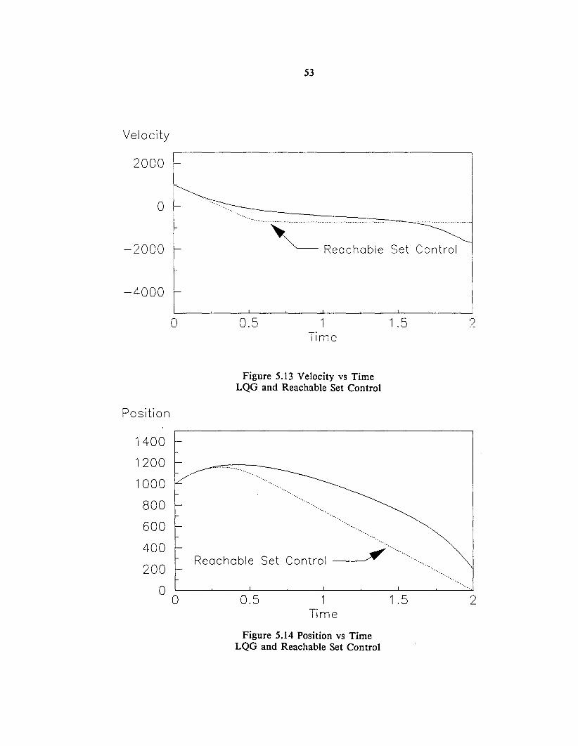
Velocity
2000
o
-2000
-4000
53
....................................................... - __ -_ .
"'-- Reachable Set Control
o 0.5 1Time
1.5 2
".
'.
Reachable Set Control~
Position
1400
1200
1000
800
600
400
200
o 0
Figure 5.13 Velocity vs TimeLQG and Reachable Set Control
" . .........
....
0.5 1Time
Figure 5.14 Position vs TimeLQG and Reachable Set Control
1.5
'"
2
54
Summary
The improved performance of Reachable Set Control is obvious from Figure
5.14. While demonstrated for a specific plant, and symmetric control constraint
set, Reachable Set Control is capable of improving the terminal performance of
a large class of systems. It minimized the effects of modeling errors (or target
set uncertainty) by regulating the system to the zero control state. The
technique handled constraints and insured an initially constrained trajectory.
The tracking problem could be optimized to the response time of the system
under consideration by smoothly driving the system from some large
displacement to a region where the relatively high gain LQG controller remained
linear.
CHAPTER VIREACHABLE SET CONTROL FOR PREFERRED AXIS HOMING MISSILES
As stated in Chapter II, the most promising techniques that can extend the
inertial point mass formulation are based on singular perturbations [37,38,39].
When applied to the preferred axis missile, each of these techniques leads to a
controller that is optimal in some sense. However, a discussion of "optimality"
notwithstanding, the best homing missile intercept trajectory is the one that
arrives at the final "control point" with the highest probability of hitting the
target. This probability can be broken down into autonomous and forced
events. If nothing is changed, what is the probability of a hit or what is the
miss distance? If the target does not maneuver, can additional control inputs
result in a hit? And, in the worse case, if the target maneuvers (or an
estimation error .is corrected) will the missile have adequate maneuverability to
correct the trajectory? None of the nonlinear techniques based on singular
perturbations attempt to control uncertainty or address the terminally
constrained trajectories caused by increasing acceleration profile.
Unfortunately, an increasing acceleration profile has been observed in all
of the preferred axis homing missile controllers. In many cases, the generic
bank-to-turn missile of [11,18] was on all three constraints (Ny,Nz,P) during the
latter portion of the trajectory. If the evading target is able to put the missile
in this position without approaching it's own maneuver limits, it will not be
possible for the missile to counter the final evasive maneuver. The missile is no
longer controllable to the target set. The "standard" solution to the increasing
acceleration profile is a varying control cost.
55
However, without additional
56
additional modifications, this type of solution results in a trajectory dependent
control. As we have seen, Reachable Set Control is an LQG control implementa
tion that moves the system to the point where further inputs are not required.
A Reachable Set Controller that will reject target and system disturbances, can
satisfy both the mathematical and heuristic optimality requirements by
minimizing the cost yet maintaining a controllable system.
Since the roll control has different characteristics, the discussion of the
preferred axis homing missile controller using the Reachable Set Control
technique will be separated into translational and roll subsystems. The
translational subsystem has a suitable null control trajectory defined by the
initial velocity and uncontrollable acceleration provided by the rocket motor.
The roll subsystem, however, is significantly different. In order for the
preferred axis missile to function, the preferred axis must be properly aligned.
Consequently, both roll angle error and roll rate should be zero at all times. In
this case, the null control trajectory collapses to the origin.
Acceleration Control
System Model
Since we want to control the relative target-missile inertial system to the
zero state, the controller will be defined in this reference frame. Each of the
individual system states are defined (in relative coordinates) as target state
minus missile state.
Begin with the deterministic system:
x(t) = Fx(t) + Gu(t) (I)
57
where
and
xyz
x = VxVyVz
u = [~~]
Since the autopilot model is a linear approximation and the inertial model
assumes instantaneous response, modeling errors will randomly affect the
trajectory. Atmospheric and other external influences will disturb the system.
Also, the determination of the state will require the use of noisy measurements.
Consequently, the missile intercept problem should be approached via a
stochastic optimal control law. Because the Reachable Set Control technique will
minimize the effect of plant parameter variations (modeling errors) and
unmodeled target maneuvers to maintain controllability, we can use an LQG
controller. Assuming Certainty Equivalence, this controller consists of an
optimal linear (Kalman) filter cascaded with the optimal feedback gain matrix of
the corresponding deterministic optimal control problem. Disturbances and
modeling errors can be accounted for by suitably extending the system
description [40]:
x(t) = F(t)x(t) + G(t)u(t) + Vs(t)
by adding a noise process Vs(·") to the dynamics equations with
(2)
(3)
58
Therefore, let the continuous time state description be formally given by the
linear stochastic differential equation
x(t) = ct>(t, to)x(to)
dx(t) = F(t)x(t)dt + G(t)u(t)dt + L(t)df3(t)
(with 13(·,.) a Wiener process) that has the solution:
ct>( t,r)G(r)u(r)dr
+ J~ <I?(I.T)L(T)dB(T)
characterized by a covariance and mean whose trajectory can be adequately
represented as:
x(t) = F(t)x(t) + G(t)u(t) + Lws(t)
where ws(''') is a zero mean white Gaussian noise of strength Ws(t) for all 1.
Disturbance Model
(4)
(5)
(6)
(7)
In the process of the intercept, it is expected that the target will attempt
to counter the missile threat. While it is theoretically possible to have an
adequate truth model and sufficiently sophisticated algorithms to adapt system
parameters or detect the maneuvers, the short time of flight and maneuver
detection delays make this approach unrealistic at this time. Even though the
actual evasive maneuvers will be discretely initiated and carried out in finite
time, the effect of these maneuvers, combined with unmodeled missile states,
appear as continuous, correlated and uninterrupted disturbances on the system.
Therefore, even though a minimum square error, unbiased estimate can be made
of the system state it would be very unusual for the estimates of the target
state to converge with zero error.
59
Since the optimal solution to the linear
stochastic differential equation is a Gauss-Markov process, time correlated
processes can be included by augmenting the system state to include the
disturbance process.
Let the time-correlated target (position) disturbance be modeled by the
following:
T(t) = N(t)T(t) + Wt(t) (8)
with
[ Tx(t)
IT(t) = Ty(t)
Tz(t)
and~{Wt(t)wt(t)T} = Wt(t)
While the target disturbance resulting from an unknown acceleration is localized
to a single plane with respect to the body axis of the target, the target
orientation is unknown to the inertial model. Consequently, following the
methodology of the Singer Model, each axis will be treated equally [41]. Since
the disturbance is first order Markov, it's components will be:
andN(t) = - (I/Tc)[I]
Wt(t) = (20't2/ Tc)[I]
(9)
(10)
where Tc is the correlation time, and O'r is the RMS value of the disturbance
process. The Power Spectral Density of the disturbance is:
Wtt(W) =20't2/ Tc
w2 + O/Tc)2(11)
Figure 6.1 summarizes the noise interactions with the system.
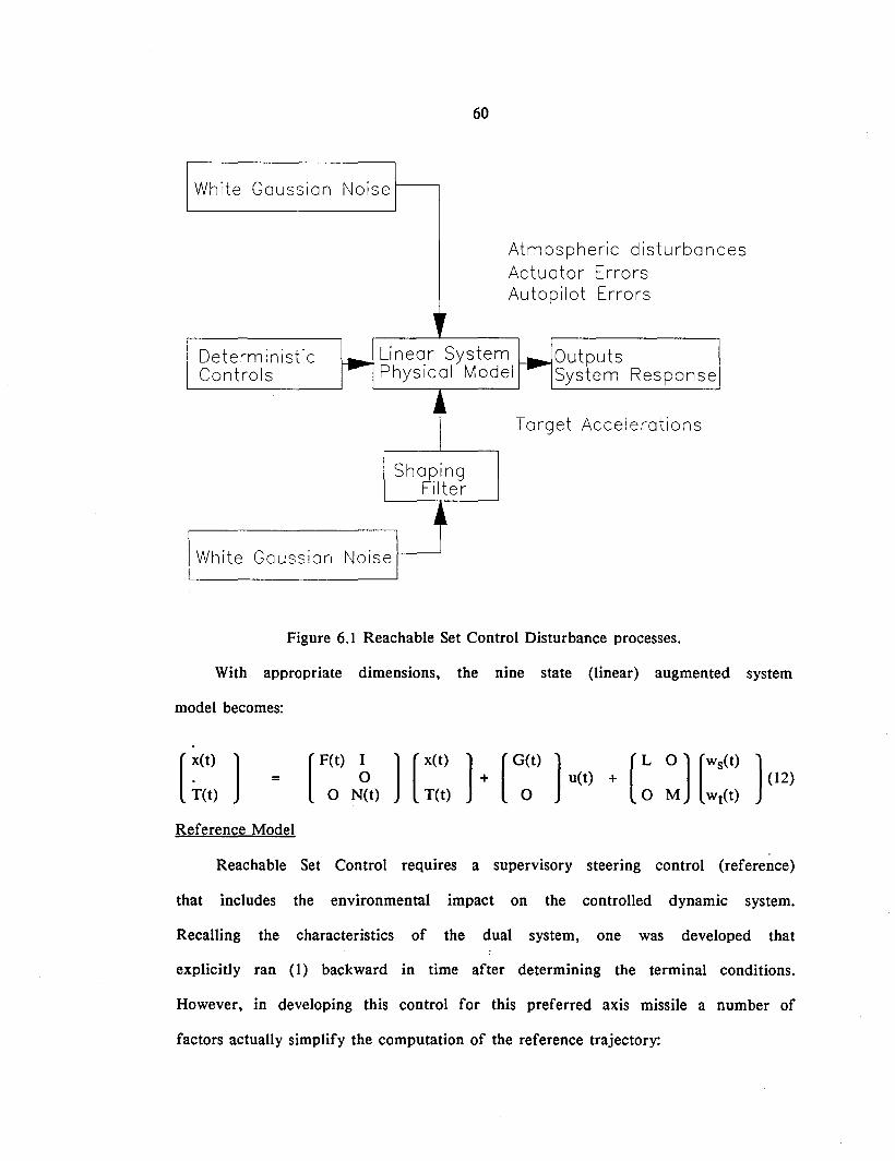
60
White Gaussian NoiseJ-------'
Atmospheric disturbancesActuator ErrorsAutopilot Errors
"DeterministicControls
~ Linear System ~ OutputsPhysical Model System Response
JlTarget Accelerations
ShapingFilter
White Gaussian Noise
Figure 6.1 Reachable Set Control Disturbance processes.
With appropriate dimensions, the nine state (linear) augmented system
model becomes:
[~(t) ]
T(t)=
Reference Model
Reachable Set Control requires a supervisory steering control (reference)
that includes the environmental impact on the controlled dynamic system.
Recalling the characteristics of the dual system, one was developed that
explicitly ran (I) backward in time after determining the terminal conditions.
However, in developing this control for this preferred axis missile a number of
factors actually simplify the computation of the reference trajectory:
61
(I) The control constraint set for this preferred axis missile is symmetric.
Consequently. the reference trajectory for an intercept condition. is a null
control (coasting) trajectory.
(2) The body axis X acceleration is provided by the missile motor, and is
not controllable but known. This uncontrollable acceleration will contribute to
the total inertial acceleration vector. must be considered by the controller. and
is the only acceleration present on an intercept (coasting) trajectory.
(3) The termination of the intercept is the closest approach. which now
becomes the fixed-final-time (tf). The time-to-go (tgo) is defined with respect
to the current time (t) by:
t = tf - tgo (13)
(4) The final boundary condition for the system state (target minus
missile) is zero.
In summary, the intercept positions are zero. the initial velocity is given.
and the average acceleration is a constant. Therefore. it is sufficient to reverse
the direction of the initial velocity and average acceleration then run the
system forward in time for tgo seconds from the origin to determine the
current position of the coasting trajectory. Let:
with
and
r(t) = A(t)r(t) + B(t)a(t)
r(O) = rO = 0
A(t) = F(t) and B(t) = G(t)
(14)
then r(t) is the point from which the autonomous system dynamics will take the
system to desired boundary condition.
Because of the disturbances. target motion, and modeling errors, future
control inputs are random vectors. Therefore, the best policy is not to
62
determine the input over the control period [to,tfl a priori but to reconsider
the situation at each instant t on the basis of all available information. At each
update, if the system is controllable, the reference (and system state) will
approach zero as tgo approaches zero.
Since the objective of the controller is to drive the system state to zero,
we do not require a tracker that will maintain the control variable at a desired
non-zero value with zero steady state error in the presence of unmodeled
constant disturbances. There are disturbances, but the final set point is zero,
and therefore, a PI controller is not required.
Roll Control
Definition
The roll mode is most significant source of modeling errors in the
preferred axis homing missile. While non-linear and high order dynamics
associated with the equations of motion, autopilot, and control actuators are
neglected, the double integrator is an exact model for determining inertial
position from inertial accelerations. The linear system, however, is referenced
with respect to the body axis. Consequently, to analyze the complete dynamics,
the angular relationship between the body axis and inertial references must be
considered. Recall Friedland's linearized (simplified) equations. The angular
relationships determine the orientation of the body axis reference and the roll
rate appeared in the dynamics of all angular relationships. Yet, to solve the
system using linear techniques, the system must be uncoupled via a steady state
(Adiabatic) assumption. Also, the roll angle is inertially defined and the effect
of the linear accelerations on the error is totally neglected.
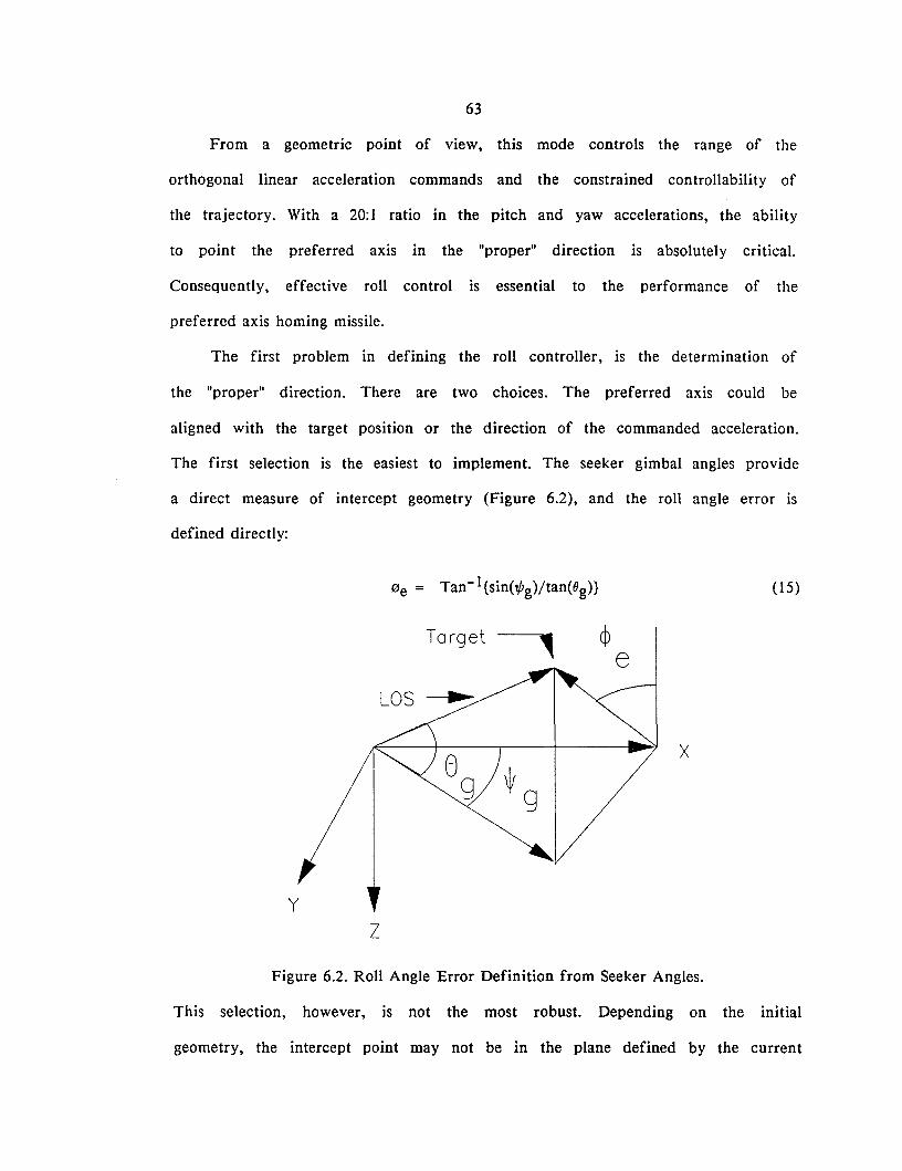
63
From a geometric point of view, this mode controls the range of the
orthogonal linear acceleration commands and the constrained controllability of
the trajectory. With a 20: I ratio in the pitch and yaw accelerations, the ability
to point the preferred axis in the "proper" direction is absolutely critical.
Consequently, effective roll control is essential to the performance of the
preferred axis homing missile.
The first problem in defining the roll controller, is the determination of
the "proper" direction. There are two choices. The preferred axis could be
aligned with the target position or the direction of the commanded acceleration.
The first selection is the easiest to implement. The seeker gimbal angles provide
a direct measure of intercept geometry (Figure 6.2), and the roll angle error is
defined directly:
(15)
Target
LOS ~
~e
y
z
x
Figure 6.2. Roll Angle Error Definition from Seeker Angles.
This selection, however, is not the most robust. Depending on the initial
geometry, the intercept point may not be in the plane defined by the current
64
line of sight (LOS) and longitudinal axis of the missile. In this case, the missile
must continually adjust its orientation (roll) to maintain the target in the
preferred plane. As range decreases the angular rates increase, with the very
real possibility of saturation and poor terminal performance.
Consequently, the second definition of roll angle error should be used.
Considering the dynamics of the intercept, however, aligning the preferred axis
with the commanded acceleration vector is not as straightforward as it seems.
Defining the roll angle error as
0 e = Tan-I{Ay/ Az} (16)
leads to significant difficulties. From the previous discussion, it is obvious that
roll angle errors must be minimized so that the preferred axis acceleration can
be used to control the intercept. The roll controller must have a high gain.
Assume, for example, the missile is on the intercept trajectory. Therefore, both
Ay and Az will be zero. Now, if the target moves slightly in the Yb direction
and the missile maneuvers to correct the deviation, the roll angle error instan
taneously becomes 90 degrees. High gain roll control inputs to correct this
situation are counter productive. The small Ay may be adequate to completely
correct the situation before the roll mode can respond. Now, the combination of
linear and roll control leads to instability as the unnecessary roll rate generates
errors in future linear accelerations.
The problems resulting from the definition of equation 16 can be overcome
be re-examining the roll angle error. First, Ay and Az combine to generate a
resultant vector at an angle from the preferred axis. In the process of applying
constraints, the acceleration angle that results from the linear accelerations can
be increased or decreased by the presence of the constraint. If the angle is
decreased, the additional roll is needed to line up the preferred axis and the
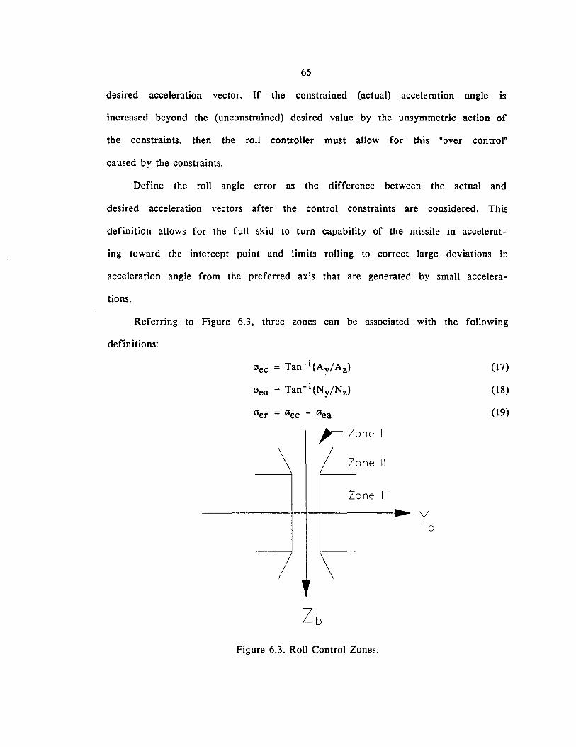
65
desired acceleration vector. If the constrained (actual) acceleration angle is
increased beyond the (unconstrained) desired value by the unsymmetric action of
the constraints, then the roll controller must allow for this "over control"
caused by the constraints.
Define the roll angle error as the difference between the actual and
desired acceleration vectors after the control constraints are considered. This
definition allows for the full skid to turn capability of the missile in accelerat
ing toward the intercept point and limits rolling to correct large deviations in
acceleration angle from the preferred axis that are generated by small accelera
tions.
Referring to Figure 6.3, three zones can be associated with the following
definitions:
"ec = Tan-I(Ay/Az}
'lea = Tan-I(Ny/Nz}
"er = "ec - 'lea
;- Zone I
Zone II
Zone III
Figure 6.3. Roll Control Zones.
(17)
(18)
(19)
66
Here Ny and Nz are the constrained acceleration values. In Zone I, "er = O.
The linear acceleration can complete the intercept without further roll angle
change. This is the desired locus for the roll controller. Both Ay and Az are
limited in Zone II. This is the typical situation for the initial position of a
demanding intercept. The objective of the roll controller is to keep the
intercept acceleration out of Zone III where only Ay is limited. In this case,
the Ay acceleration is insufficient to complete the intercept yet significant roll
angle change may be required to make the trajectory controllable.
Controller
A dual mode roll controller was developed to accommodate the range of
situations and minimize roll angle error. Zone I requires a lower gain controller
that will stabilize the roll rate and maintain "er small. Zones II and III require
high gain controllers. To keep Zone II trajectories from entering Zone III, the
"ec will be controlled to zero rather than the roll angle error. Since the linear
control value is also a function of the roll angle error, roll angle errors are
determined by comparing the desired and actual angles of a fixed high gain
reachable set controller. If the actual linear commands are used and a linear
acceleration is small because of large roll angle errors, the actual amount of
roll needed to line up the preferred axis and the intercept point, beyond the
capability of the linear accelerations, will not be available because they have
been limited by the existing roll angle error that must be corrected.
Unlike the inertial motions, the linear model for the roll controller
accounts for the (roll) damping and recognizes that the input is a roll rate
change command:
" = -w" + wP (20)
67
Therefore, the roll mode elements (that will be incorporated into the model are)
are:
(21)
Also, the dual mode controller will require an output function and weighting
matrix that includes both roll angle and roll rate.
Kalman Filter
The augmented system model (13) is not block diagonal. Consequently, the
augmented system filter will not decouple into two independent system and
reference filters. Rather, a single, higher order filter was required to generate
the state and disturbance estimates.
A target model (the Singer model) was selected and modified to track ma-
neuvering targets from a Bank-To-Turn missile [41,42]. Using this model, a
continuous-discrete Extended Kalman Filter was developed. The filter used a 9
state target model for the relative motion (target - missile):
(22)
with u(t) the known missile acceleration, N the correlation coefficient, and
Wt(t) an assumed Gaussian white noise input with zero mean.
Azimuth, elevation, range, and range rate measurements were available
from passive JR, semi-active, analog radar, and digitally processed radar sensors.
The four measurements are seeker azimuth (,p), seeker elevation (0), range (r),
and range rate (dr/dt):
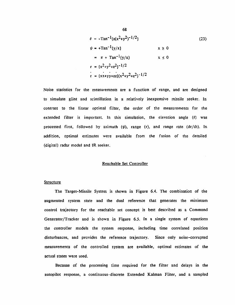
68
6 = - Tan- l{z(x2+y2)-1/2}
t/J = +Tan-l{y/x}
= 1r + Tan-l{y/x}
r = {x2+y2+z2}-1/2
r = {x~+y~+z~}{x2+y2+z2}-1/2
x ~ 0
x ~ 0
(23)
Noise statistics for the measurements are a function of range, and are designed
to simulate glint and scintillation in a relatively inexpensive missile seeker. In
contrast to the linear optimal filter, the order of the measurements for the
extended filter is important. In this simulation, the elevation angle (6) was
processed first, followed by azimuth (t/J), range (r), and range rate (dr/dt). In
addition, optimal estimates were available from the fusion of the detailed
(digital) radar model and IR seeker.
Reachable Set Controller
Structure
The Target-Missile System is shown in Figure 6.4. The combination of the
augmented system state and the dual reference that generates the minimum
control trajectory for the reachable set concept is best described as a Command
Generator/Tracker and is shown in Figure 6.5. In a single system of equations
the controller models the system response, including time correlated position
disturbances, and provides the reference trajectory. Since only noise-corrupted
measurements of the controlled system are available, optimal estimates of the
actual states were used.
Because of the processing time required for the filter and delays in the
autopilot response, a continuous-discrete Extended Kalman Filter, and a sampled
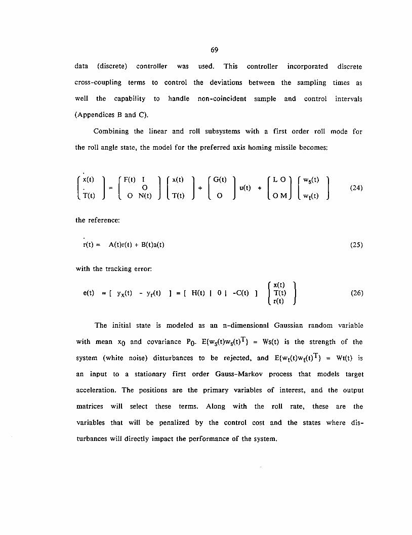
69
data (discrete) controller was used. This controller incorporated discrete
cross-coupling terms to control the deviations between the sampling times as
well the capability to handle non-coincident sample and control intervals
(Appendices B and C).
Combining the linear and roll subsystems with a first order roll mode for
the roll angle state, the model for the preferred axis homing missile becomes:
the reference:
r(t) = A(t)r(t) + B(t)a(t)
with the tracking error:
e(t) = [ yx(t) - Yr(t) ] = [ H(t) I 0 I -C(t)] [~W»)r(t)
(25)
(26)
The initial state is modeled as an n-dimensional Gaussian random variable
with mean xO and covariance PO. E{ws(t)ws(t)T} = Ws(t) is the strength of the
system (white noise) disturbances to be rejected, and E{wt(t)Wt(t)T} = Wt(t) is
an input to a stationary first order Gauss-Markov process that models target
acceleration. The positions are the primary variables of interest, and the output
matrices will select these terms. Along with the roll rate, these are the
variables that will be penalized by the control cost and the states where dis-
turbances will directly impact the performance of the system.
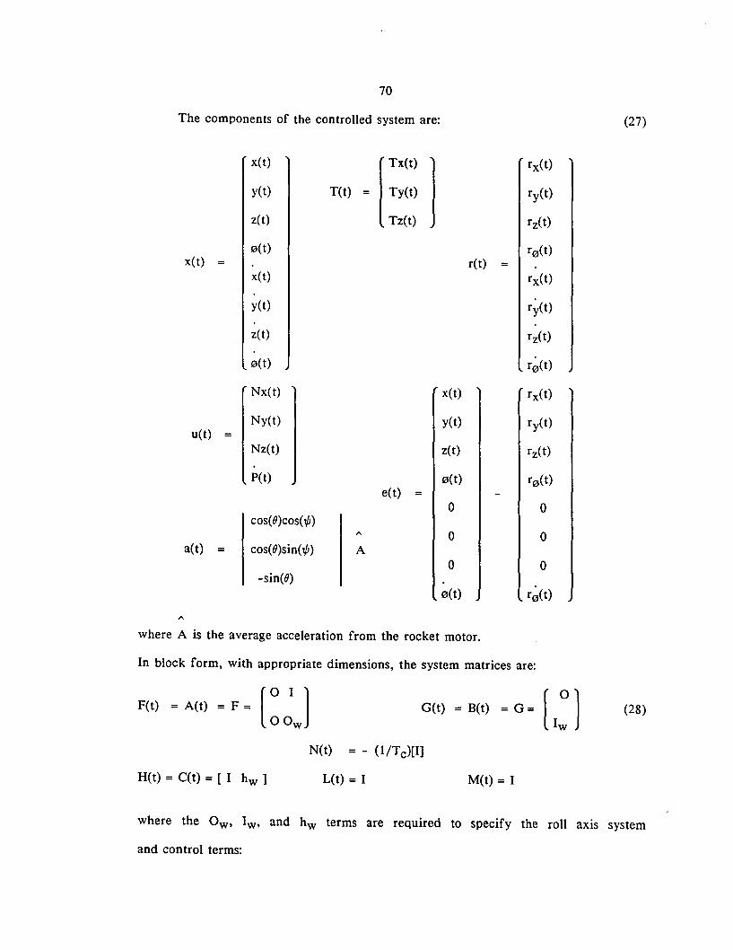
In block form, with appropriate dimensions, the system matrices are:
F(t) = A(t) = F = [0 I ]OOw
G(t) = B(t) = G = [ 0]I w
(28)
H(t) = C(t) = [I hw ]
N(t) = - (ljTc)[I]
L(t) = I M(t) = I
where the Ow, Iw, and hw terms are required to specify the roll axis system
and control terms:
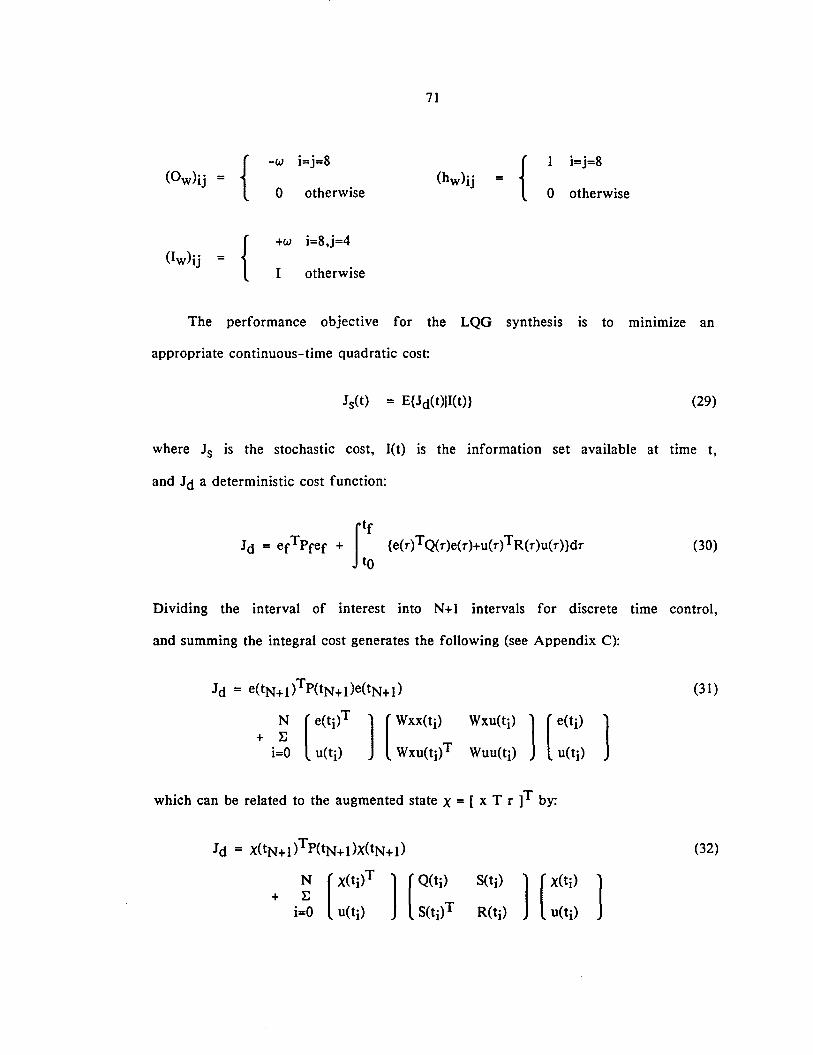
71
{ -w i=j=8 { 1 i=j=8(Ow>ij = (hw>ij =
0 otherwise 0 otherwise
{ +w i=8,j=4(Iw)ij =
I otherwise
The performance objective for the LQG synthesis is to minimize an
appropriate continuous-time quadratic cost:
Js(t) = E{Jd(t)II(t)} (29)
where Js is the stochastic cost, I(t) is the information set available at time t,
and Jd a deterministic cost function:
(30)
Dividing the interval of interest into N+I intervals for discrete time control,
and summing the integral cost generates the following (see Appendix C):
(31 )
which can be related to the augmented state X = [ x T r ]T by:
] [
X(tj)
u(ti) ](32)
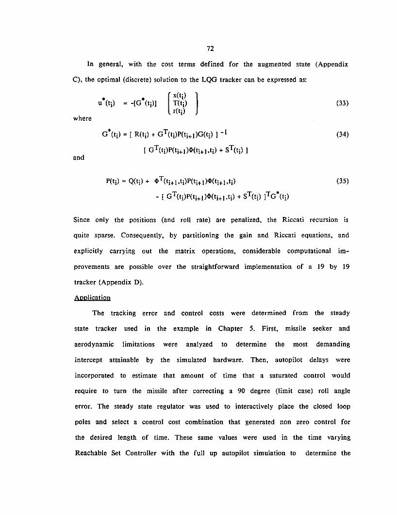
72
In general, with the cost terms defined for the augmented state (Appendix
C), the optimal (discrete) solution to the LQG tracker can be expressed as:
where
*= -[G (ti)][
x(ti)T(ti)r(ti) ] (33)
and
G*(ti) = [ R(ti) + GT(ti)P(ti+l)G(ti) ] -1
[ GT(ti)P(ti+l)~(ti+J,ti) + ST(tj) ]
P(ti) = Q(ti) + ~T(ti+l,ti)P(ti+l)~(ti+J,ti)
- [ GT(ti)P(ti+I)~(ti+l,ti) + ST(ti) ]TG*(ti)
(34)
(35)
Since only the positions (and roll rate) are penalized, the Riccati recursion is
quite sparse. Consequently, by partitioning the gain and Riccati equations, and
explicitly carrying out the matrix operations, considerable computational im-
provements are possible over the straightforward implementation of a 19 by 19
tracker (Appendix D).
Application
The tracking error and control costs were determined from the steady
state tracker used in the example in Chapter 5. First, missile seeker and
aerodynamic limitations were analyzed to determine the most demanding
intercept attainable by the simulated hardware. Then, autopilot delays were
incorporated to estimate that amount of time that a saturated control would
require to turn the missile after correcting a 90 degree (limit case) roll angle
error. The steady state regulator was used to interactively place the closed loop
poles and select a control cost combination that generated non zero control for
the desired length of time. These same values were used in the time varying
Reachable Set Controller with the full up autopilot simulation to determine the
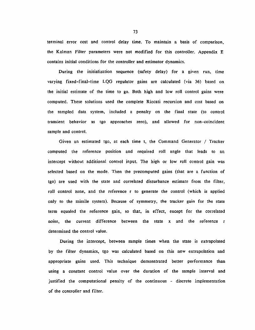
73
terminal error cost and control delay time. To maintain a basis of comparison,
the Kalman Filter parameters were not modified for this controller. Appendix E
contains initial conditions for the controller and estimator dynamics.
During the initialization sequence (safety delay) for a given run, time
varying fixed-final-time LQG regulator gains are calculated (via 36) based on
the initial estimate of the time to go. Both high and low roll control gains were
computed. These solutions used the complete Riccati recursion and cost based on
the sampled data system, included a penalty on the final state (to control
transient behavior as tgo approaches zero), and allowed for non-coincident
sample and control.
Given an estimated tgo, at each time t, the Command Generator I Tracker
computed the reference position and required roll angle that leads to an
intercept without additional control input. The high or low roll control gain was
selected based on the mode. Then the precomputed gains (that are a function of
tgo) are used with the state and correlated disturbance estimate from the filter,
roll control zone, and the reference r to generate the control (which is applied
only to the missile system). Because of symmetry, the tracker gain for the state
term equaled the reference gain, so that, in effect, except for the correlated
noise, the current difference between the state x and the reference r
determined the control value.
During the intercept, between sample times when the state is extrapolated
by the filter dynamics, tgo was calculated based on this new extrapolation and
appropriate gains used. This technique demonstrated better performance than
using a constant control value over the duration of the sample interval and
justified the computational penalty of the continuous - discrete implementation
of the controller and filter.
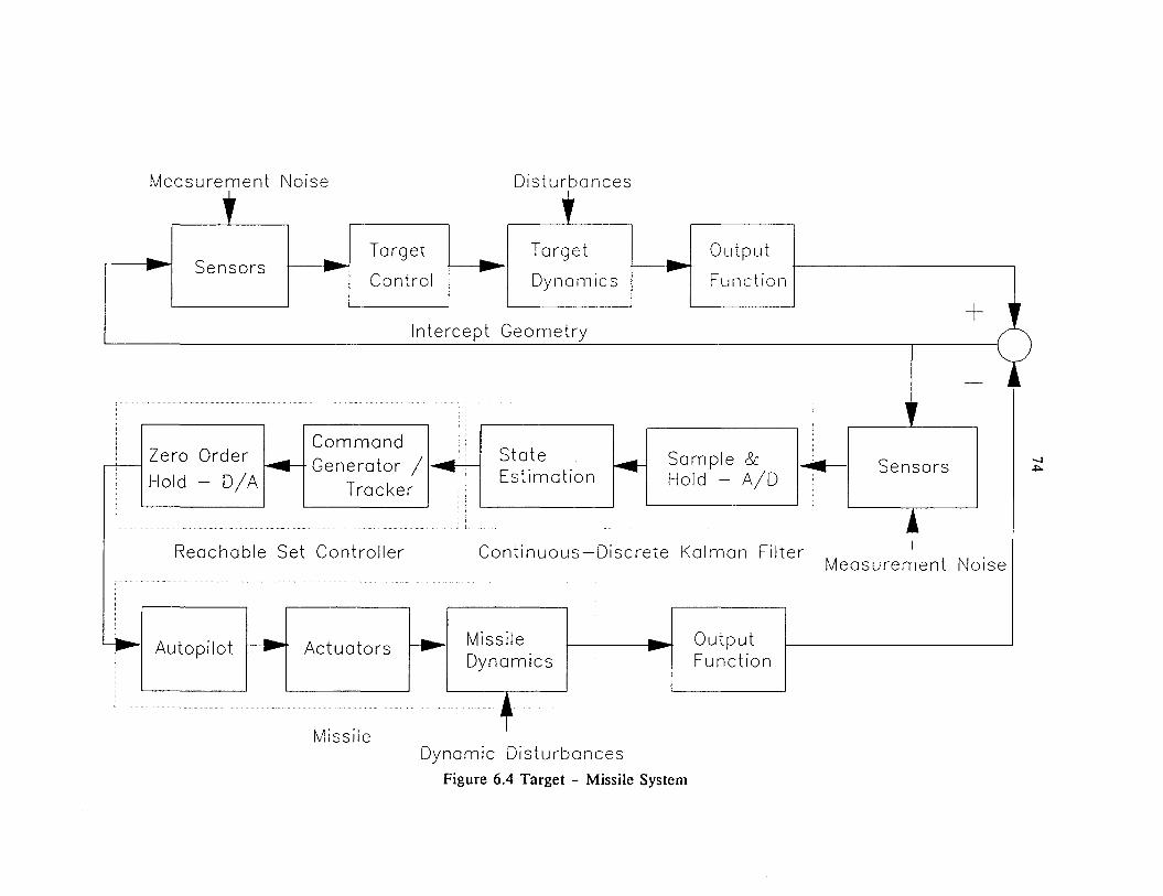
Measurement Noise,Intercept Geometry
-- Sensors -- Target
Control--
Disturbances,Target
Dynamics-- Output
Function
+ "
l'Command
-- Zero Order ~ Generator I ..Hold - DI A Tracker
StateEstimation
Sample &Hold - AID
Sensors
Reachable Set Controller Continuous-Discrete Kalman FilterMeasurement Noise
'-~ Autopilot -- Actuators ~
Missile
MissileDynamics
-- OutputFunction
Dynamic DisturbancesFigure 6.4 Target - Missile System
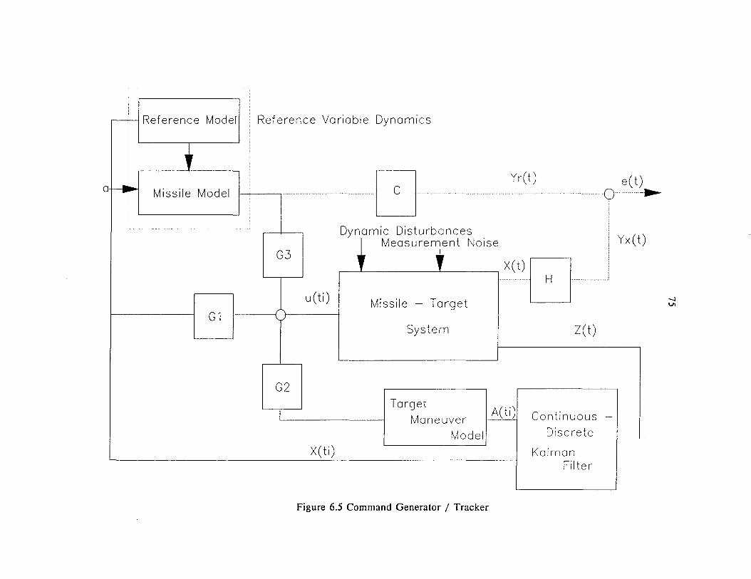
r-- Reference Model Reference Variable Dynamics
a .... Missile Model~ Yr(t) e(t),----,···························LJ ·····················0--
Dynamic DisturbancesMeasurement Noise
" ,G1
G3
u(ti)I---{ "')-------1
G2
Missile - Target
System
X(t)Q !················LJ i
Z( t)
Yx(t)
X( ti)
TargetManeuver
Model
A( ti) Continuous Discrete
KalmanFilter
-
Figure 6.5 Command Generator / Tracker
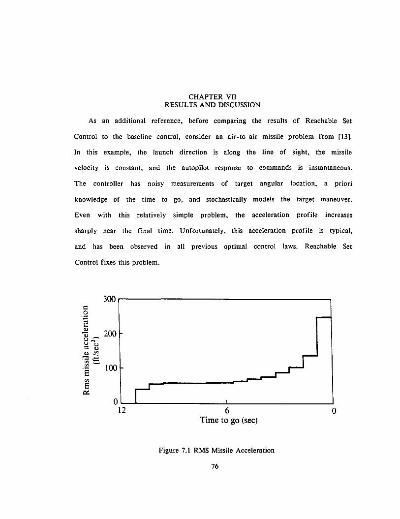
CHAPTER VIIRESULTS AND DISCUSSION
As an additional reference, before comparing the results of Reachable Set
Control to the baseline control, consider an air-to-air missile problem from [13].
In this example, the launch direction is along the line of sight, the missile
velocity is constant, and the autopilot response to commands is instantaneous.
The controller has noisy measurements of target angular location, a priori
knowledge of the time to go, and stochastically models the target maneuver.
Even with this relatively simple problem, the acceleration profile increases
sharply near the final time. Unfortunately, this acceleration profile is typical,
and has been observed in all previous optimal control laws. Reachable Set
Control fixes this problem.
c.9-~...oa:)_u '"u u~ 0o en--.... t=~-.-EenE
0=:
300r-------------------~
200
100
o6Time to go (sec)
O'--....L----- -l-. ---l
12
Figure 7.1 RMS Missile Acceleration
76
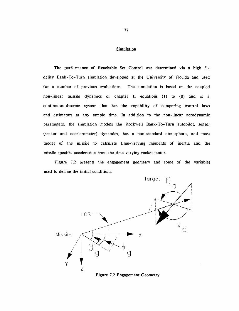
77
Simulation
The performance of Reachable Set Control was determined via a high fi-
delity Bank-To-Turn simulation developed at the University of Florida and used
for a number of previous evaluations. The simulation is based on the coupled
non-linear missile dynamics of chapter II equations (1) to (8) and is a
continuous-discrete system that has the capability of comparing control laws
and estimators at any sample time. In addition to the non-linear aerodynamic
parameters, the simulation models the Rockwell Bank-To-Turn autopilot, sensor
(seeker and accelerometer) dynamics, has a non-standard atmosphere, and mass
model of the missile to calculate time-varying moments of inertia and the
missile specific acceleration from the time varying rocket motor.
Figure 7.2 presents the engagement geometry and some of the variables
used to define the initial conditions.
Missile
y,Z
Target Ga
xD .....~\IfU 9 ;./ \j! 9
Figure 7.2 Engagement Geometry
78
The simulated target is a three (3) dimensional, nine (9) "g" maneuvering
target. Initially, the target trajectory is a straight line. Once the range from
the missile to target is less than 6000 feet, the target initiates an instantaneous
9 "g" evasive maneuver in a plane determined by the target roll angle, an input
parameter. If the launch range is within 6000 feet, the evasive maneuver begins
immediately. There is a .4 second "safety" delay between missile launch and
autopilot control authority.
Trajectory Parameters
The performance of the control laws was measured with and without sensor
noise using continuous and sampled data measurements. The integration step was
.005 seconds and the measurement step for the Extended Kalman Filter was .05
seconds. The trajectory presented for comparison has an initial offset angle of
40 degrees (tPg) and 180 degree aspect (tPa), and a target roll of 90 degrees away
from the missile. This angle off and target maneuver is one of the most
demanding intercept for a preferred axis missile since it must roll through 90
degrees before the preferred axis is aligned with the target. Other intercepts
were run with different conditions and target maneuvers to verify the
robustness of Reachable Set Control and the miss distances were similar or less
that this trajectory.
Results
Deterministic Results
These results are the best comparison of control concepts since both
Linear Optimal Control and Reachable Set Control are based on assumed Cer
tainty Equivalence.
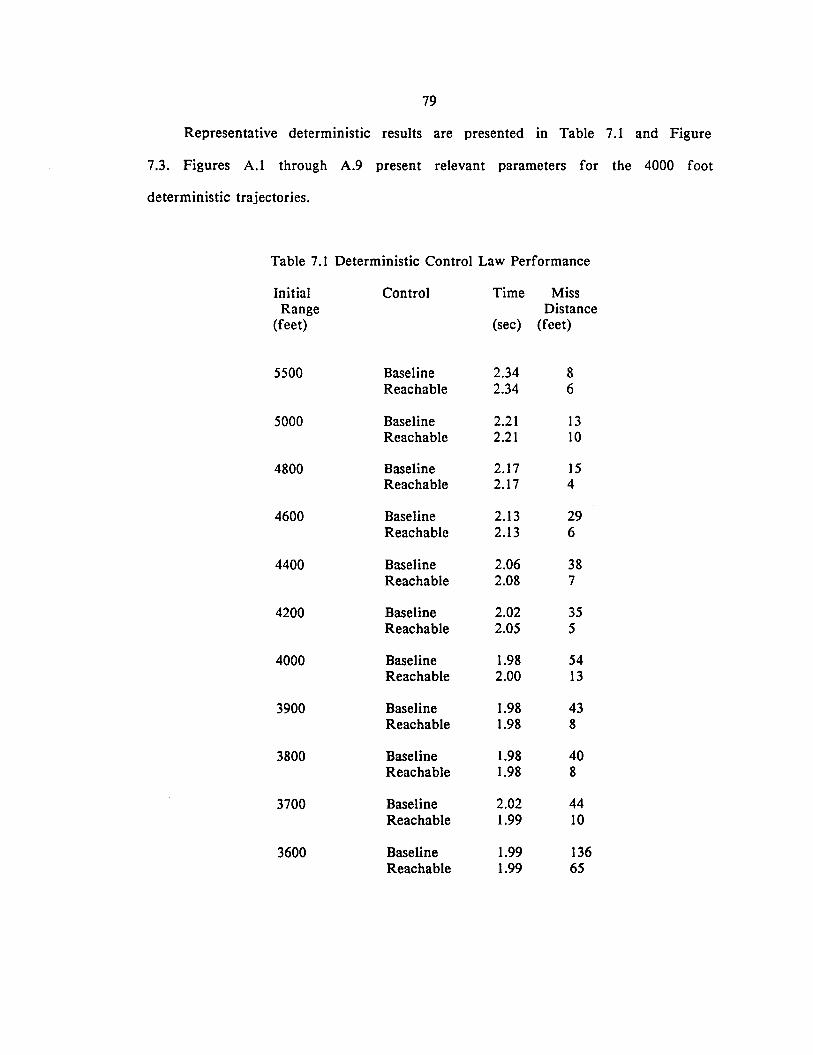
79
Representative deterministic results are presented in Table 7.1 and Figure
7.3. Figures A.l through A.9 present relevant parameters for the 4000 foot
deterministic trajectories.
Table 7.1 Deterministic Control Law Performance
Initial Control Time MissRange Distance
(feet) (sec) (feet)
5500 Baseline 2.34 8Reachable 2.34 6
5000 Baseline 2.21 13Reachable 2.21 10
4800 Baseline 2.17 15Reachable 2.17 4
4600 Baseline 2.13 29Reachable 2.13 6
4400 Baseline 2.06 38Reachable 2.08 7
4200 Baseline 2.02 35Reachable 2.05 5
4000 Baseline 1.98 54Reachable 2.00 13
3900 Baseline 1.98 43Reachable 1.98 8
3800 Baseline 1.98 40Reachable 1.98 8
3700 Baseline 2.02 44Reachable 1.99 10
3600 Baseline 1.99 136Reachable 1.99 65
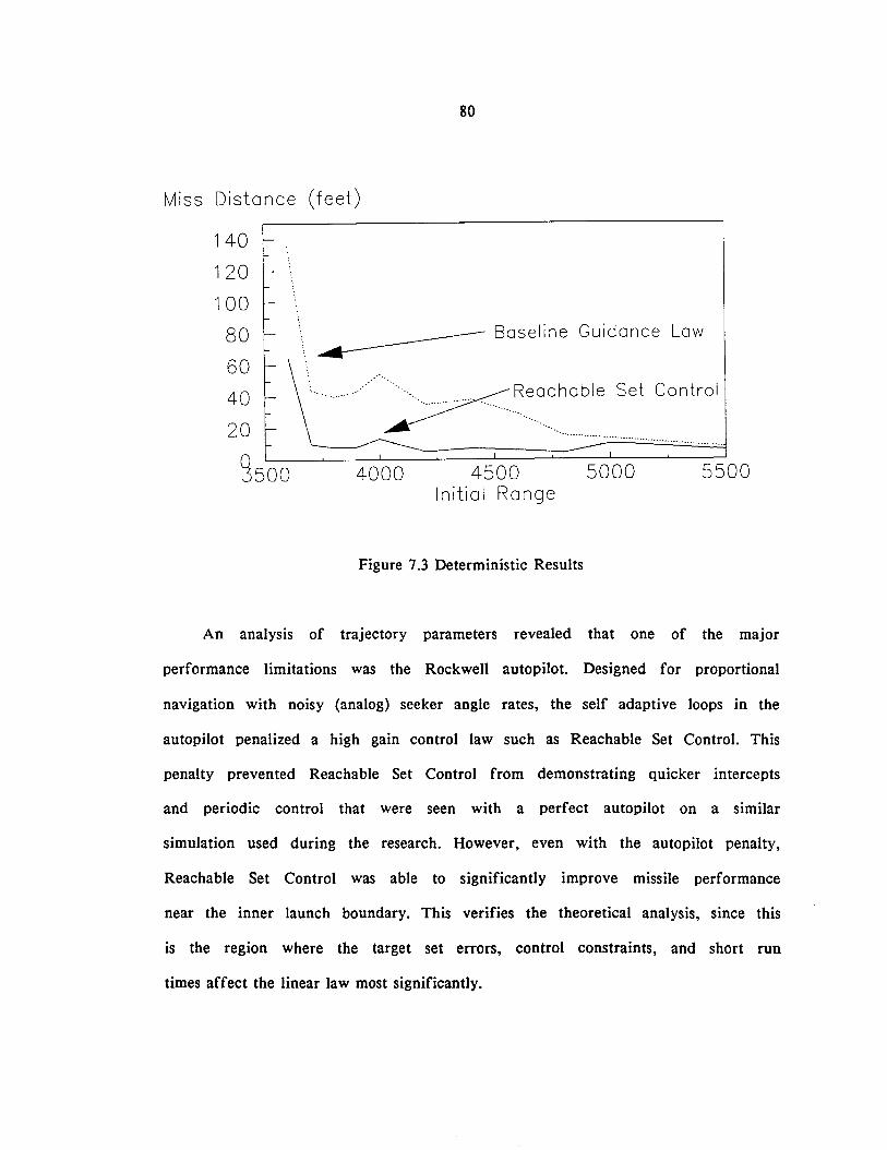
80
Miss Distance (feet)
~ Baseline Guidance Law
............. / ~~eO~hOble Set Control
140 f--
120 -
100 -
80 f--
60 -
40 -
20 e-
j500 4000 4500Initial Range
5000 5500
Figure 7.3 Deterministic Results
An analysis of trajectory parameters revealed that one of the major
performance limitations was the Rockwell autopilot. Designed for proportional
navigation with noisy (analog) seeker angle rates, the self adaptive loops in the
autopilot penalized a high gain control law such as Reachable Set Control. This
penalty prevented Reachable Set Control from demonstrating quicker intercepts
and periodic control that were seen with a perfect autopilot on a similar
simulation used during the research. However, even with the autopilot penalty,
Reachable Set Control was able to significantly improve missile performance
near the inner launch boundary. This verifies the theoretical analysis, since this
is the region where the target set errors, control constraints, and short run
times affect the linear law most significantly.
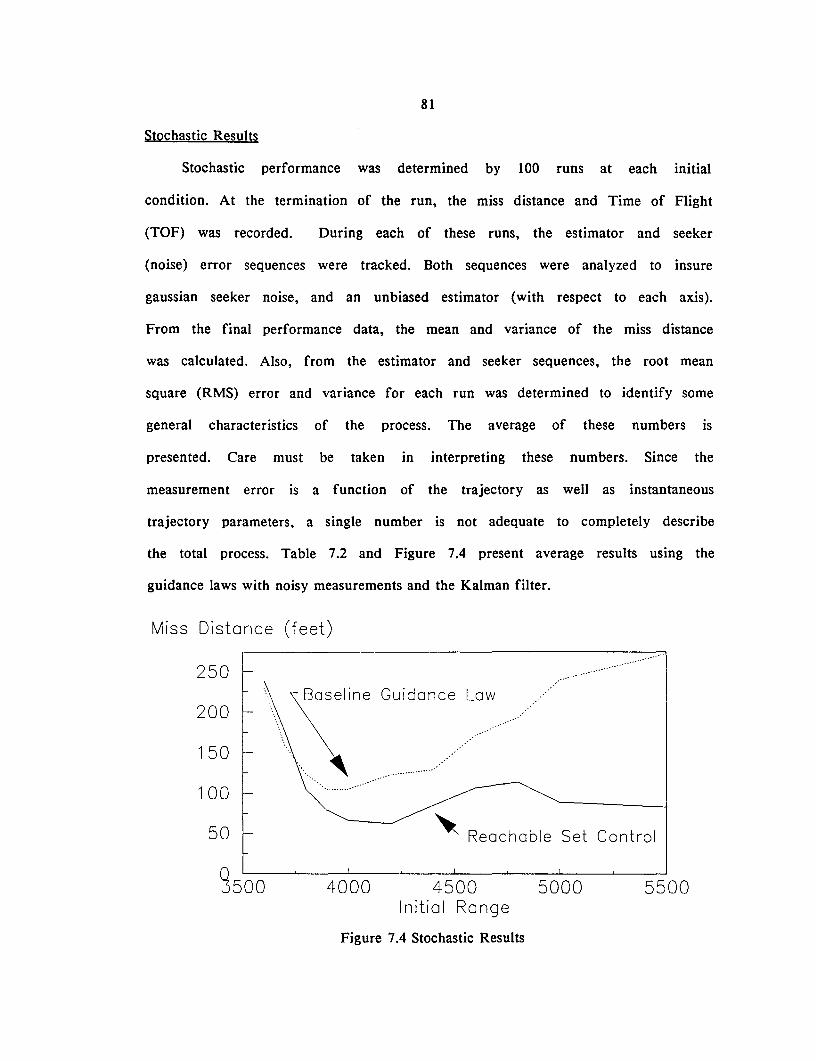
81
Stochastic Results
Stochastic performance was determined by 100 runs at each initial
condition. At the termination of the run, the miss distance and Time of Flight
(TOF) was recorded. During each of these runs, the estimator and seeker
(noise) error sequences were tracked. Both sequences were analyzed to insure
gaussian seeker noise, and an unbiased estimator (with respect to each axis).
From the final performance data, the mean and variance of the miss distance
was calculated. Also, from the estimator and seeker sequences, the root mean
square (RMS) error and variance for each run was determined to identify some
general characteristics of the process. The average of these numbers is
presented. Care must be taken in interpreting these numbers. Since the
measurement error is a function of the trajectory as well as instantaneous
trajectory parameters, a single number is not adequate to completely describe
the total process. Table 7.2 and Figure 7.4 present average results using the
guidance laws with noisy measurements and the Kalman filter.
Miss Distance (feet)
250
200
150
100
Baseline Guidance Law
.. , ..'
.,.....
50 " Reachable Set Control
S500 4000 4500Initial Range
5000 5500
Figure 7.4 Stochastic Results
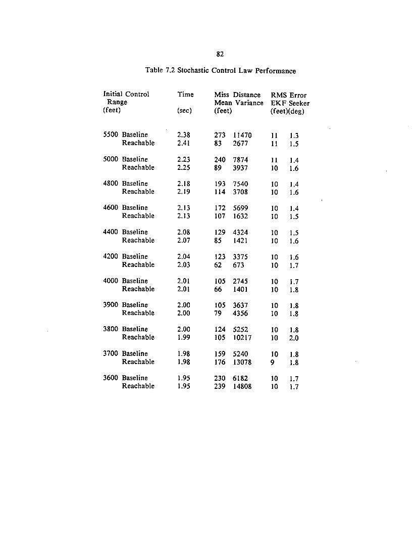
82
Table 7.2 Stochastic Control Law Performance
Initial Control Time Miss Distance RMS ErrorRange Mean Variance EKF Seeker
(feet) (sec) (feet) (feet)(deg)
5500 Baseline 2.38 273 11470 11 1.3Reachable 2.41 83 2677 11 1.5
5000 Baseline 2.23 240 7874 11 1.4Reachable 2.25 89 3937 10 1.6
4800 Baseline 2.18 193 7540 10 1.4Reachable 2.19 114 3708 10 1.6
4600 Baseline 2.13 172 5699 10 1.4Reachable 2.13 107 1632 10 1.5
4400 Baseline 2.08 129 4324 10 1.5Reachable 2.07 85 1421 10 1.6
4200 Baseline 2.04 123 3375 10 1.6Reachable 2.03 62 673 10 1.7
4000 Baseline 2.01 105 2745 10 1.7Reachable 2.01 66 1401 10 1.8
3900 Baseline 2.00 105 3637 10 1.8Reachable 2.00 79 4356 10 1.8
3800 Baseline 2.00 124 5252 10 1.8Reachable 1.99 105 10217 10 2.0
3700 Baseline 1.98 159 5240 10 1.8Reachable 1.98 176 13078 9 1.8
3600 Baseline 1.95 230 6182 10 1.7Reachable 1.95 239 14808 10 1.7
83
The first runs made with Reachable Set Control were not as good as the
results presented. Reachable Set Control was only slightly (10 to 20 feet)
superior to the baseline guidance law and was well below expectations. Yet, the
performance of the filter with respect to position error was reasonable, many of
the individual runs had miss distances near 20 feet, and most of the errors
were in the Z axis. Analyzing several trajectories from various initial conditions
led to two main conclusions. First, the initial and terminal seeker errors were
quite large, especially compared to the constant 5 mrad tracking accuracy
assumed by many studies [2,3,18]. Second, the non-linear coupled nature of the
preferred axis missile, combined with range dependent seeker errors, and the
system (target) model, makes the terminal performance a strong function of the
particular sequence of seeker errors. For example, Figure 7.5 compares the
actual and estimated Z axis velocity (Target - Missile) from a single 4000 foot
run. The very first elevation measurement generated a 14 foot Z axis position
error. A reasonable number considering the range. The Z axis velocity error,
however, was quite large, 409 feet per second, and never completely eliminated
by the filter. Recalling that the target velocity is 969 feet per second, is
approximately co-altitude with the missile and maneuvers primarily in the XY
plane, this error is significant when compared to the actual Z axis velocity (2
feet per second). Also, this is the axis that defines the roll angle error and,
consequently, roll rate of the missile. Errors of this magnitude cause the
primary maneuver plane of the missile to roll away from the target limiting (via
the constraints) the ability of the missile to maneuver.
Further investigation confirmed that the filter was working properly.
Although the time varying noise prevents a direct comparison for an entire
trajectory, these large velocity errors are consistent with the covariance ratios
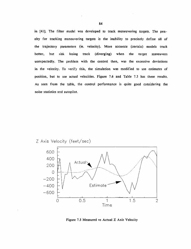
84
in [41]. The filter model was developed to track maneuvering targets. The pen-
alty for tracking maneuvering targets is the inability to precisely define all of
the trajectory parameters (ie. velocity). More accurate (certain) models track
better, but risk losing track (diverging) when the target maneuvers
unexpectedly. The problem with the control then, was the excessive deviations
in the velocity. To verify this, the simulation was modified to use estimates of
position, but to use actual velocities. Figure 7.6 and Table 7.3 has these results.
As seen from the table, the control performance is quite good considering the
noise statistics and autopilot.
Z Axis Velocity (feet/sec)
600
400
200Actual,
0
-200
-400
-600
0 0.5 1 1.5 2Time
Figure 7.5 Measured vs Actual Z Axis Velocity
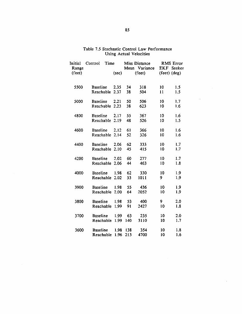
85
Table 7.5 Stochastic Control Law PerformanceUsing Actual Velocities
Initial Control Time Miss Distance RMS ErrorRange Mean Variance EKF Seeker(feet) (sec) (feet) (feet) (deg)
5500 Baseline 2.35 34 318 10 1.5Reachable 2.37 38 504 II 1.5
5000 Baseline 2.21 50 506 10 1.7Reachable 2.23 38 623 10 1.6
4800 Baseline 2.17 55 367 10 1.6Reachable 2.19 48 526 10 1.5
4600 Baseline 2.12 61 366 10 1.6Reachable 2.14 52 326 10 1.6
4400 Baseline 2.06 62 333 10 1.7Reachable 2.10 45 415 10 1.7
4200 Baseline 2.02 60 277 10 1.7Reachable 2.06 44 463 10 1.8
4000 Baseline 1.98 62 330 10 1.9Reachable 2.02 53 lOll 9 1.9
3900 Baseline 1.98 55 436 10 1.9Reachable 2.00 64 2052 10 1.9
3800 Baseline 1.98 53 400 9 2.0Reachable 1.99 91 2427 10 1.8
3700 Baseline 1.99 63 235 10 2.0Reachable 1.99 140 3110 10 1.7
3600 Baseline 1.98 138 354 10 1.8Reachable 1.96 213 4700 10 1.6
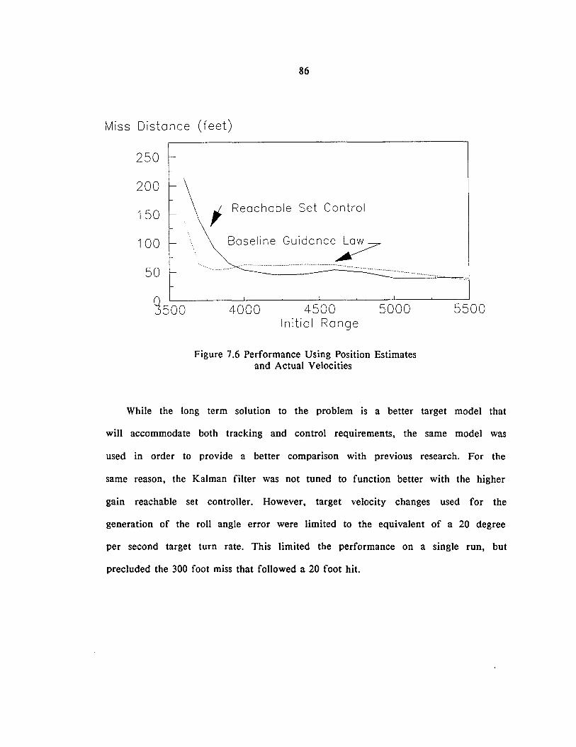
86
Miss Distance (feet)
250
200
150
100
50
,. Reachable Set Control
Baseline GUidance/
...................................................-------_ ... ------
9500 4000 4500Initial Range
5000 5500
Figure 7.6 Performance Using Position Estimatesand Actual Velocities
While the long term solution to the problem is a better target model that
will accommodate both tracking and control requirements, the same model was
used in order to provide a better comparison with previous research. For the
same reason, the Kalman filter was not tuned to function better with the higher
gain reachable set controller. However, target velocity changes used for the
generation of the roll angle error were limited to the equivalent of a 20 degree
per second target turn rate. This limited the performance on a single run, but
precluded the 300 foot miss that followed a 20 foot hit.
87
Conclusions
Reachable Set Control
As seen from the Tables 7.1 and 7.2, Reachable Set Control was inherently
more accurate than the baseline linear law, especially in the more realistic case
where noise is added and sampled data measurements are used.
In addition, Reachable set control did insure an initially constrained
trajectory for controllable trajectories, and required minimal accelerations
during the terminal phase of the intercept.
Unlike previous constrained control schemes, Reachable Set Control was
better able to accommodate tinmodeled non-linearities and provide adequate
performance with a suboptimal sampled data controller.
While demonstrated with a Preferred Axis Missile, Reachable Set Control is
a general technique that could be used on most trajectory control problems.
Singer Model
Unmodified, the Singer model provides an excellent basis for a maneuver
ing target tracker, but it is not a good model to use for linear control. Neither
control law penalized velocity errors. In fact, the baseline control law did not
define a velocity error. Yet the requirements of linearity, and the integration
from velocity to position, require better velocities estimates than are provided
by this model (for this quality seeker).

APPENDIX ASIMULAnON RESULTS
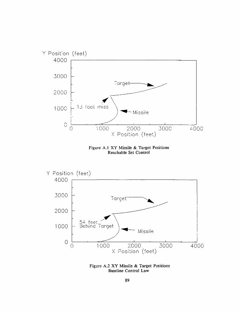
Y Position (feet)4000
3000Targe~
2000
1000
o 0
~13 foot miss
~Missile
1000 2000 3000X Position (feet)
Figure A.l XY Missile & Target PositionsReachable Set Control
4000
Y Position (feet)4000
3000Target~
2000
54 feet ~1000 Behind Target
o 0 1000 2000 3000X Position (feet)
Figure A.2 XY Missile & Target PositionsBaseline Control Law
89
4000
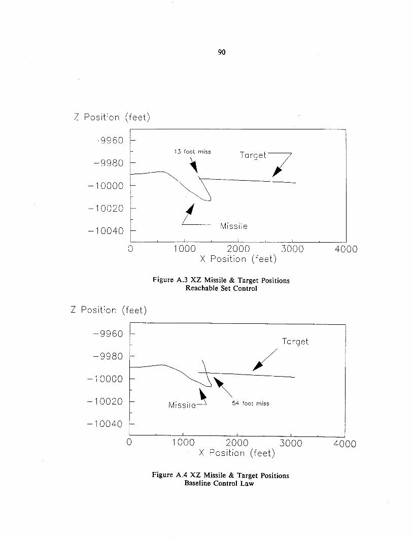
90
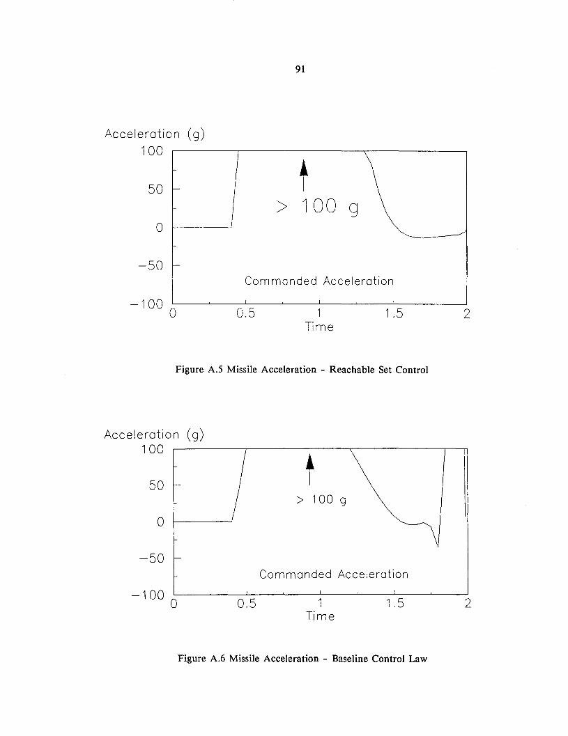
91
Acceleration (g)100
50 -
o
-50 f-
t> 100 9
Commanded Acceleration
-100 o 0.5 1Time
1.5 2
Figure A.S Missile Acceleration - Reachable Set Control
Acceleration (g)100
50
o
-50
,I
> 100 9
Commanded Acceleration
-100 o 0.5 1Time
1.5 2
Figure A.6 Missile Acceleration - Baseline Control Law
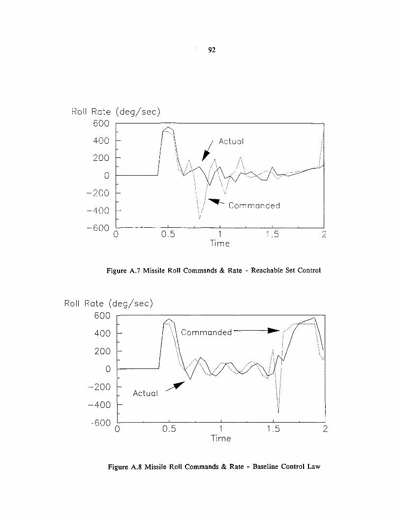
92
Roll Rate (deg/sec)600
400
200
0
-200
-400
-6000 0.5 1
Time
...
1.5 2
Figure A.7 Missile Roll Commands & Rate - Reachable Set Control
Actual
Ro II Rate (deg/sec)
600
400
200
o-200
-400
Commanded-----~
'.:
-600 o 0.5 1Time
1.5 2
Figure A.8 Missile Roll Commands & Rate - Baseline Control Law
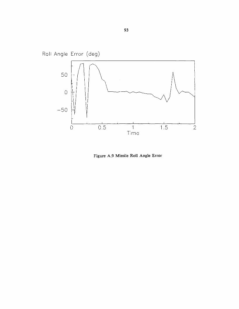
93
Roll Angle Error (deg)
50
o
-50
o 0.5 1Time
1.5 2
Figure A.9 Missile Roll Angle Error
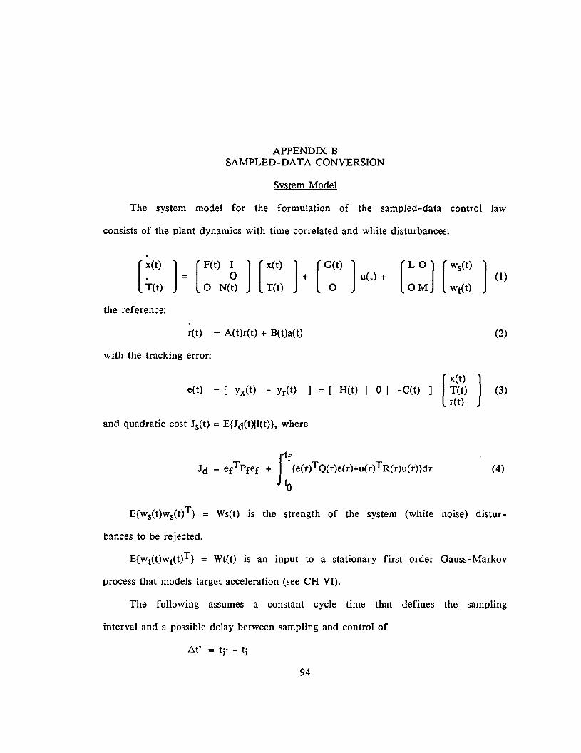
APPENDIX BSAMPLED-DATA CONVERSION
System Model
The system model for the formulation of the sampled-data control law
consists of the plant dynamics with time correlated and white disturbances:
[~(t) ] = [F(t) ~ ] [X(t) ] + [GO(t) ] u(t) +T(t) 0 N(t) T(t)
the reference:
r(t) = A(t)r(t) + B(t)a(t)
with the tracking error:
[L0] [WS(t) ] (1)
OM Wt(t)
(2)
e(t) = [ yx(t) - Yr(t) ] = [ H(t) I 0 I -C(t) ] [~W) ) (3)r(t)
and quadratic cost Js(t) = E{Jd(t)II(t)}, where
(4)
E{ws(t)ws(t)T} = Ws(t) is the strength of the system (white noise) distur-
bances to be rejected.
E{wt(t)Wt(t)T} = Wt(t) is an input to a stationary first order Gauss-Markov
process that models target acceleration (see CH VI).
The following assumes a constant cycle time that defines the sampling
interval and a possible delay between sampling and control of
~t' = ti' - ti
94
9S
The components of the controlled system are
x(t) =
x(t)
y(t)
Z(t)
0(t)
x(t)
T(t) = [::::: ]
Tz(t)
r(t)
(5)
o 0
u(t)
y(t)
z(t)
0(t)
Nx(t)
Ny(t)
Nz(t)
P(t)e(t)
x(t)
y(t)
z(t)
0(t)
ry(t)
rz(t)
r0 (t)
rx(t)
ry(t)
rz(t)
r0 (t)
o 0
o 0
In block form, with appropriate dimensions, the system matrices are
F(t) = A(t) = F = [0 I ]
° OwG(t) = B(t) = G = [~w] (6)
H(t) = C(t) = [I hw ]
i=j=8
otherwise
{
+w i=8,j=4(Iw)ij =
I otherwise
L(t) = I
(hw)jj = { ~
M(t) = I
i=j=8
otherwise
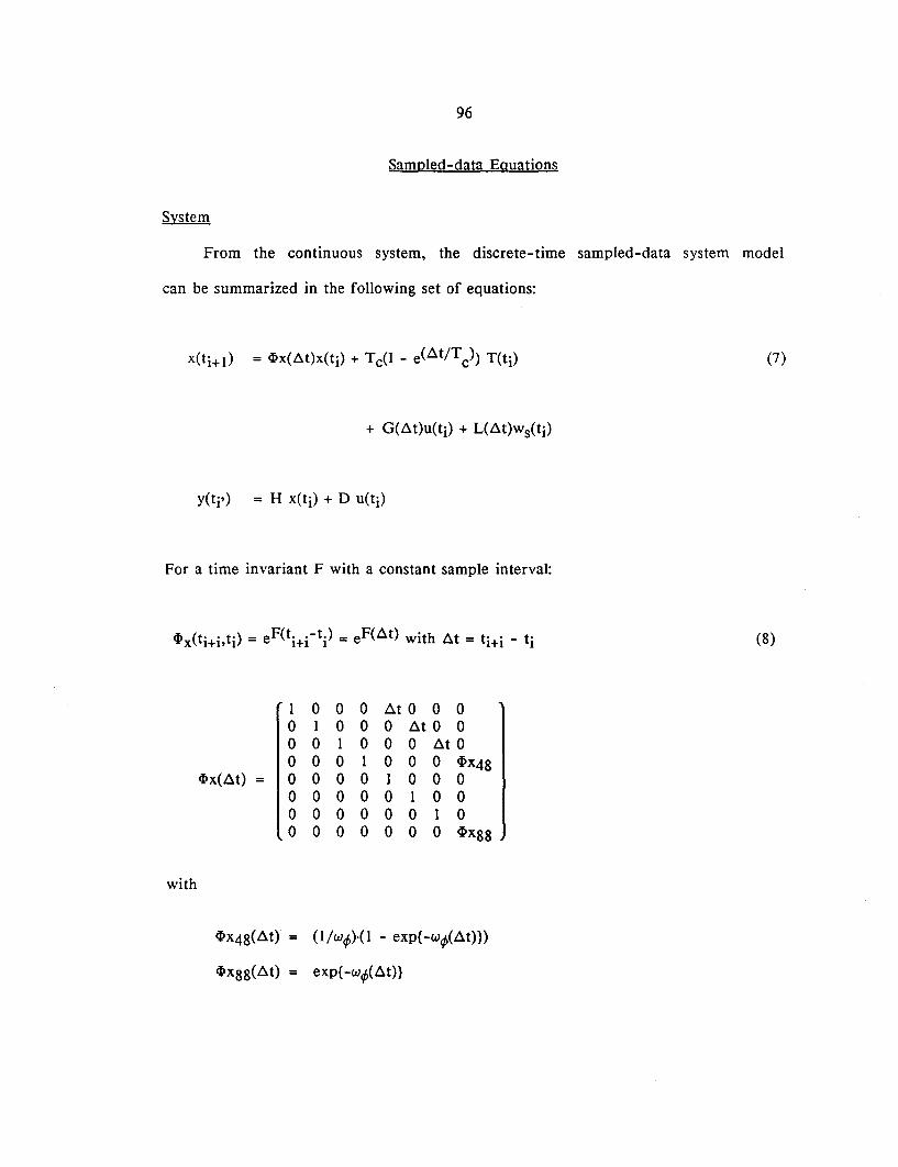
96
Sampled-data Equations
System
From the continuous system, the discrete-time sampled-data system model
can be summarized in the following set of equations:
y(ti') = H x(ti) + D u(ti)
For a time invariant F with a constant sample interval:
<I> (t· . t·) - eF(t..-1.) - eF(.£lt) with .£lt - t·· t·x HI' 1 - HI 1 - - HI - 1
I 0 0 0 .£lt 0 0 00 I 0 0 0 .£ltO 00 0 I 0 0 0 .£ltO0 0 0 I 0 0 0 <I>x48
<I>x(.£lt) = 0 0 0 0 I 0 0 00 0 0 0 0 I 0 00 0 0 0 0 0 I 00 0 0 0 0 0 0 <I>x88
with
<I>x48(.£lt) = (l!w</».(l - exp{-w</>(.£lt)})
<I>x88(.£lt) = exp{ -w</>(.£lt)}
(7)
(8)
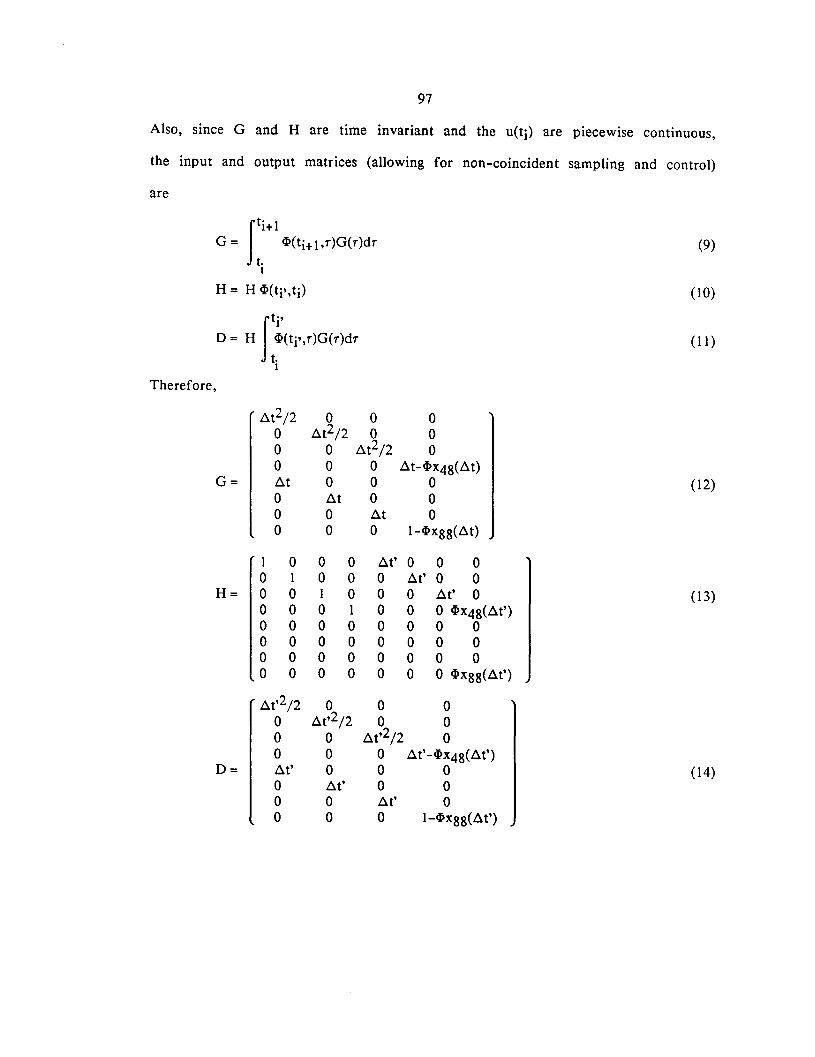
97
Also, since G and H are time invariant and the u(ti) are piecewise continuous,
the input and output matrices (allowing for non-coincident sampling and control)
are
fi+lG= cP(ti+l,r)G(r)dr (9)t.1
H = H cP(ti',ti) (10)
rD = H ~(tj"r)G(r)dr (11 )t.1
Therefore,
At2j2 0 0 00 At2j2 0 00 0 At2j2 00 0 0 At-cPx4S(At)
G= At 0 0 0 (12)0 At 0 00 0 At 00 0 0 l-cPxSS(At)
I 0 0 0 At' 0 0 00 I 0 0 0 At' 0 0
H= 0 0 I 0 0 0 At' 0 (13)0 0 0 I 0 0 o cPX4S(At')0 0 0 0 0 0 0 00 0 0 0 0 0 0 00 0 0 0 0 0 0 00 0 0 0 0 0 o cPXSS(At')
At,2 j2 0 0 00 At,2j 2 0 00 0 At,2j2 00 0 0 At' -cPX4S(At')
D= At' 0 0 0 (14)0 At' 0 00 0 At' 00 0 0 l-cPxSS(At')
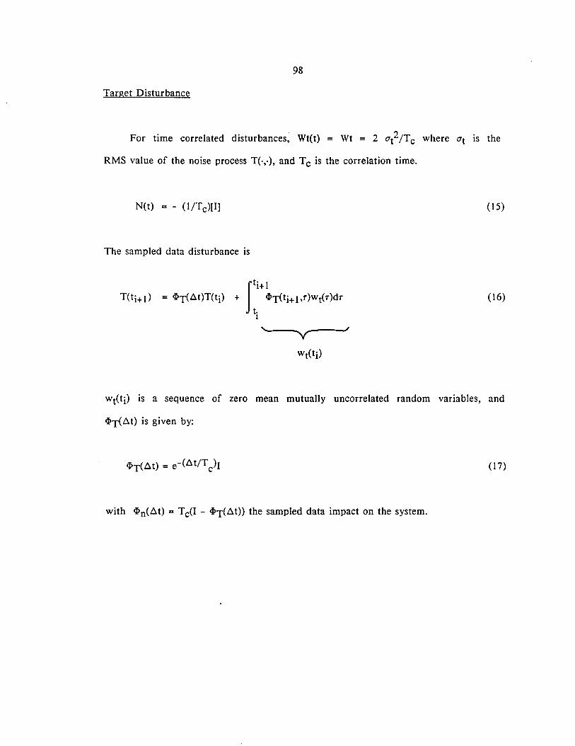
98
Target Disturbance
For time correlated disturbances, Wt(t) = Wt = 2 at2ITc where at is the
RMS value of the noise process T(·,.), and Tc is the correlation time.
N(t) = - (1/Tc)[I]
The sampled data disturbance is
(15)
(16)
Wt(ti) is a sequence of zero mean mutually uncorrelated random variables, and
<PT(~t) is given by:
with <pn(~t) = Tc(l - <PT(~t» the sampled data impact on the system.
(17)
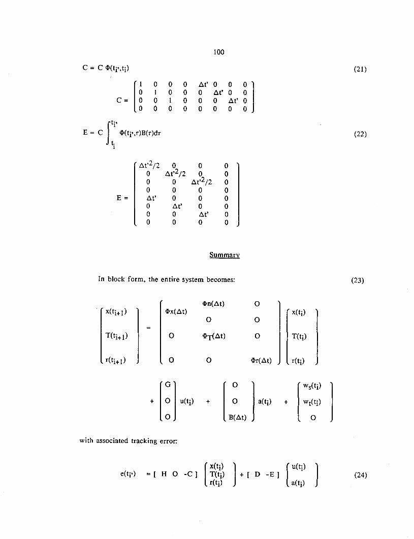
100
C = C <P(ti',ti) (21 )
C = [~0 0 0 ~t' 0 0
~ ]I 0 0 0 ~t' 00 I 0 0 0 ~t'
0 0 0 0 0 0
rE = C 1 <p(ti',r)B(r)dr (22)t.1
~t'2/2 0 0 00 ~t,2/2 0 00 0 ~t'2/2 00 0 0 0
E= ~t' 0 0 00 ~t' 0 00 0 ~t' 00 0 0 0
Summary
In block form, the entire system becomes:
<pn(~t) 0x(ti+l) <px(~t) x(ti)
0 0=
T(ti+l) 0 <PT(~t) 0 T(ti)
r(ti+l) 0 0 <pr(~t) r(ti)
(23)
with associated tracking error:
[B~al) ).(Ii) [
ws(ti) )
+ Wt(ti)
o
[
x(ti) ] [ u(tj)= [ H 0 -C] T(ti) + [ D - E ]
r(ti) a(ti) ] (24)
APPENDIX CSAMPLED DATA COST FUNCTIONS
Assume that the performance objective is to minimize an appropriate
continuous-time quadratic cost.
(1)
where Js is the stochastic cost, Jd a deterministic cost, and I(t) is the
information set available at time t.
Let
Jd(t) = erTPrer + rr(e(t)TQ(t)e(')+u(t)TR(t)u(t»dT
to(2)
Dividing the interval of interest into N+l control intervals for discrete time
control,
Jd(t) = e(tn+l)TPfe(tn+l)
N Jti+1+ i~ [ t {e(t)TQ(t)e(t) + u(t)TR(t)u(t)}dr]
1
where for all t E [tj,ti+l)' u(t) = u(ti).
Substituting the following for e(t):
(3)
e(t) = ~(t,ti)e(ti) + Jt~(t,r)G(r)U(r)drt.1
+ Jt ~(t,r)L(r)dJ3(r)ti
101
(4)
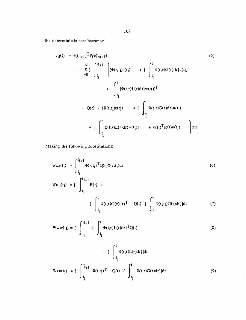
102
the deterministic cost becomes:
(5)
+NE [
i=O Jti+1 [
[4>(t, ti)e(ti)
t·I
+ { Jt 4>(t,r)G(r)dr}u(ti)
t.1
+ Jt {4>(t,r)L(r)dr}w(ti)]T
t.1
+ { It 4>(t,r)G(r)dr}u(ti)
t.I
+ { It 4>(t,r)L(r)dr}w(ti)]
t.1
Making the following substitutions:
(6)
{ It 4>(t,r)G(r)dr}T
t.1
Q(t) { Jr 4>(r,ti)G(r)dr}]dt
.t1
(7)
J'i+l r'l;(t,T)L(T)dT}TQ(t)Www(ti) = [ {
t. t.I 1
. { r'l;(t,T)L(T)dT}]dt
t.1
f+l 4>(t,ti)T 1:Wxu(ti) = [ Q(t) { 4>(t,r)G(r)dr}]dt
t.1 1
(8)
(9)
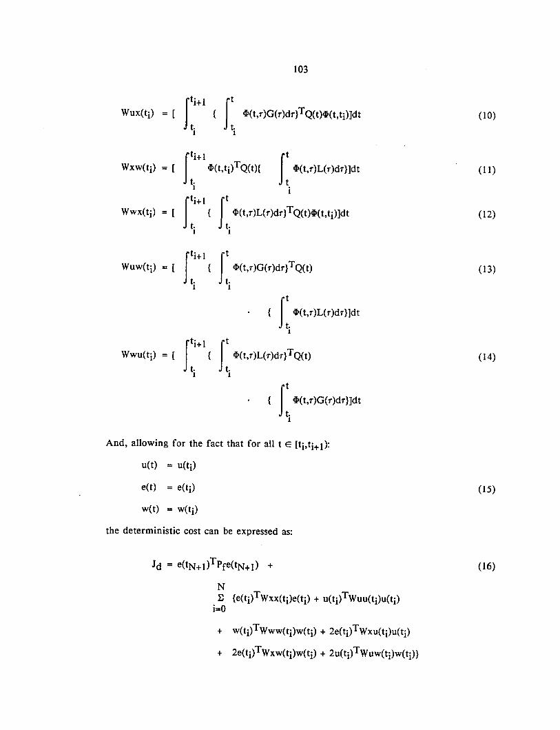
103
fi+1 J: ~(t,T)L(T)dT)]dtWxw(ti) = [ ~(t,ti)1r~(t){
t.1 i
WWX(ti) = [ f+' ( f ~(t,T)L(T)dT)TQ(t)~(t,ti)ldtt. t.1 1
WUW(ti) = [ fi+1 ( f ~(t,T)G(T)dT)TQ(t)t. t.1 1
( f ~(t,T}L(T}dT)]dtt.1
WWU(ti) = [ fi+' ( f ~(t,T)L(T)dT)TQ(t)t. t.1 1
( f ~(t,T}G(T}dT)]dtt.1
And, allowing for the fact that for all t E [ti,ti+l):
u(t) = u(ti)
e(t) = e(ti)
w(t) = w(ti)
the deterministic cost can be expressed as:
Jd = e(tN+1)1rPfe(tN+l) +
NE (e(ti)1rWxx(ti)e(ti) + u(ti)1rWuu(ti)u(ti)
i=O
+ W(ti)1rWWW(ti)W(ti) + 2e(ti)1rWXU(ti)U(ti)
+ 2e(ti)1rWXW(ti)W(ti) + 2u(ti)1rWUW(ti)W(ti)}
(10)
(11)
(12)
(13)
(14)
(15)
(16)
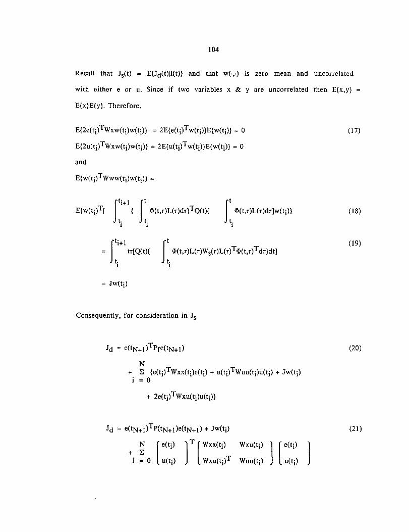
104
Recall that Js(t) = E{Jd(t)II(t)} and that w(.,.) is zero mean and uncorrelated
with either e or u. Since if two variables x & yare uncorrelated then E{x,y} =
E{x}E{y}. Therefore,
E{2e(ti)TWxw(ti)W(ti)} = 2E{e(ti)Tw(ti)}E{w(ti)} = 0
E{2u(ti)TWxw(ti)W(ti)} = 2E{u(ti)Tw(ti)}E{w(ti)} = 0
and
(17)
Jt ~(t,r)L(r)dr)w(ti)}t.1
(18)
Jt i+1
= tr[Q(t){
t.1
Jt ~(t,r)L(r)Ws(r)L(r)T~(t,r)Tdr}dt)
t.1
(19)
Consequently, for consideration in Js
Jd = e(tN+l)TPfe(tN+l)
N+ E (e(ti)TWxx(ti)e(ti) + U(ti)TWuu(ti)U(ti) + Jw(ti)
1 = 0
(20)
Wxu(ti)
Wuu(ti)
(21)
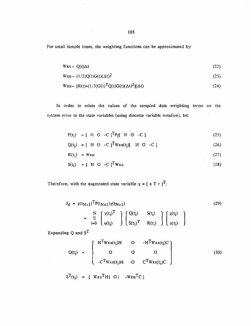
105
For small sample times, the weighting functions can be approximated by:
Wxx- Q(t).M
Wxu- (I/2)Q(t)G(t)(.6.t)2
Wuu- [R(t)+( I13 )G( t)TQ(t)G(t)(.6.t)2](.6.t)
(22)
(23)
(24)
In order to relate the values of the sampled data weighting terms on the
system error to the state variables (using discrete variable notation), let:
P(ti) = [ H 0 -C]Tpr[ H 0 -C] (25)
Q(ti) = [ H 0 -C ]TWxx(ti)[ H 0 -C] (26)
R(ti) = Wuu (27)
S(ti) =[ H 0 -C ]TWxu (28)
Therefore, with the augmented state variable X = [ x T r ]T:
Expanding Q and ST
](29)
[
HTWX~(ti)H
-CTWXX(ti)H
o
o
o
-HTW~X(ti)C ]
CTWXX(ti)C
(30)
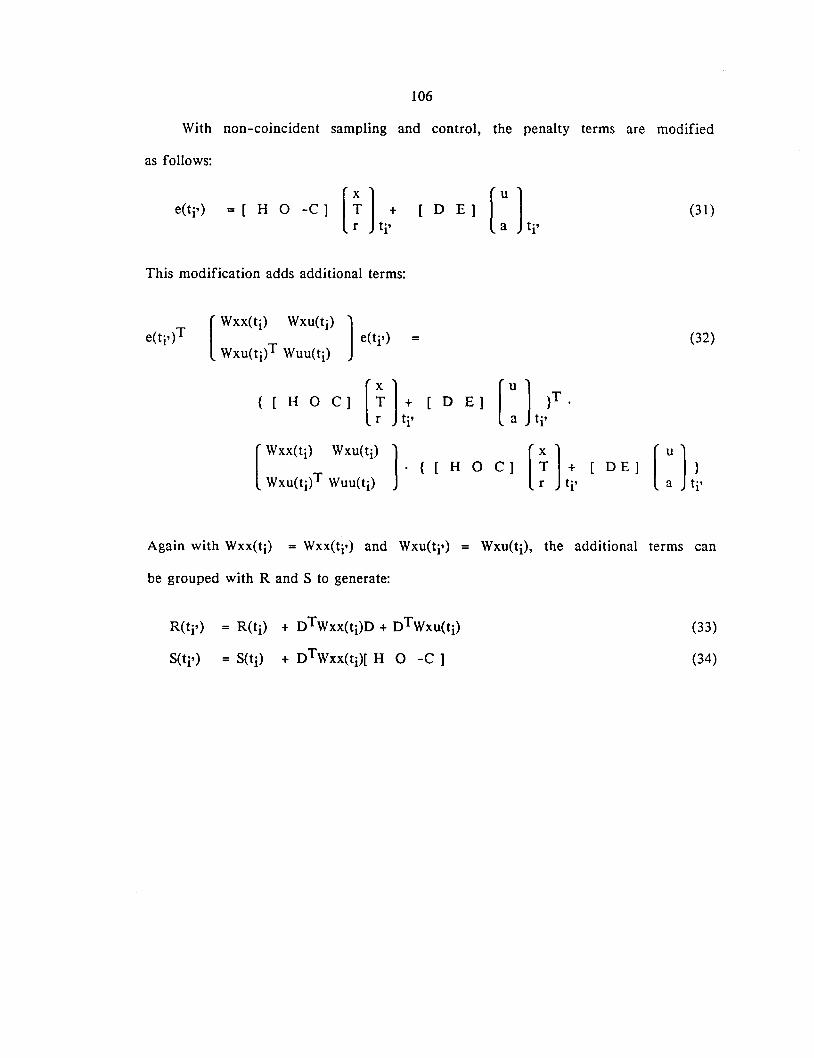
106
With non-coincident sampling and control, the penalty terms are modified
as follows:
e(ti') = [ H 0 -C] [~] +r ti'
This modification adds additional terms:
[D E] [U]a ti'
(31 )
(32)
{ [ HOC] [~] + [ DE] [U] }T.r ti' a ti'
C] [~]+ [DE] [U]}r ti' a ti'
Again with Wxx(ti) = Wxx(ti') and Wxu(ti') = Wxu(ti), the additional terms can
be grouped with Rand S to generate:
R(ti') = R(ti) + DTWxx(ti)D + DTWxu(ti)
S(ti') = S(ti) + DTWxx(ti)[ H 0 -C]
(33)
(34)
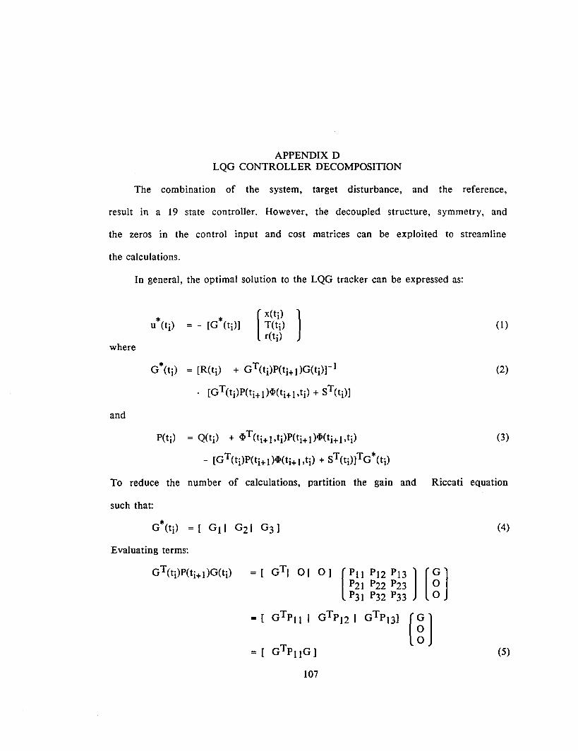
APPENDIX DLQG CONTROLLER DECOMPOSITION
The combination of the system, target disturbance, and the reference,
result in a 19 state controller. However, the decoupled structure, symmetry, and
the zeros in the control input and cost matrices can be exploited to streamline
the calculations.
In general, the optimal solution to the LQG tracker can be expressed as:
where
and
G*(ti) = [R(ti) + GT(ti)P(ti+l)G(ti)r l
. [GT(ti)P(ti+l)cI>(ti+l,ti) + ST(ti)]
P(ti) = Q(ti) + cI>T(ti+}.ti)P(ti+l)cI>(ti+l,ti)
- [GT(ti)P(ti+l)cI>(ti+}.ti) + ST(ti)]TG*(ti)
(I)
(2)
(3)
To reduce the number of calculations, partition the gain and Riccati equation
such that:
Evaluating terms:
(4)
GT(ti)P(ti+ 1)G(til = [
= [
= [
GT1 0 I 0] [PI I Pl2 P13 ] [G]P21 P22 P23 0P31 P32 P33 0
GTPII I GTPI2 I GTP13J [g]GTPIIG]
107
(5)
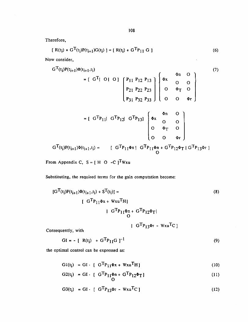
108
Therefore,
Now consider,
GT(ti)P(ti+ 1)~(ti+ I,ti)~n 0
= [ GT1 01 0] [PII P12 P13j ~x0 0
P21 P22 P23 0 ~T 0
P31 P32 P33 0 0 ~r
~n 0= [ GTPIII GTPl21 GTP13] ~x
0 0
0 ~T 0
0 0 ~r
(6)
(7)
[ GTP11~X I GTP11~n + GTPI2~T I GTP13~r]o
From Appendix C, S = [H 0 -C ]TWxu
Substituting, the required terms for the gain computation become:
[GT(ti)P(ti+I)~(ti+1 ,ti) + ST(ti)) =
GTP11~X + WxuTHI
GTPII~n + GTPI2~TIo
(8)
Consequently, with
(9)
the optimal control can be expressed as:
G1(ti) = GI· GTP11~X + WxuTH]
G2(tj) = GI· GTP11~n+ GTPI2~T]0
G3(ti) = GI· GTP13~r - WxuTC]
(10)
(11)
(12)
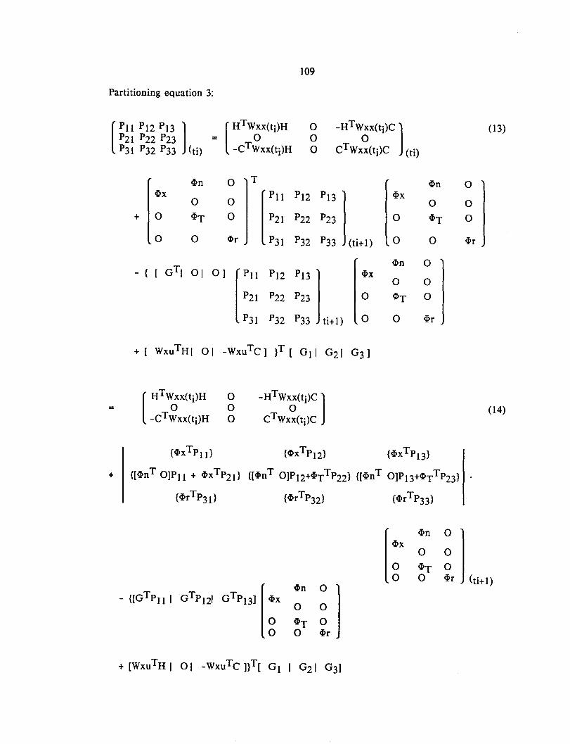
109
Partitioning equation 3:
[PH PI2 Pl3 ] [ HTW~X('i)H 0 -HTWXX('i)C] (13)P21 P22 P23 = 0
CTWX~(ti)C (ti)P31 P32 P33 (ti) -CTWXX(ti)H 0
4>n 0 T 4>n 04>x
[ PI I P12 Pl314>x
0 0 0 0+ 0 4>T 0 P21 P22 P23 0 4>T 0
0 0 4>r P31 P32 P33 (ti+1) 0 0 4>r
4>n 0- ( [ GTI 01
01 [PI I PI2 Pl3 ]4>x
0 0
P2I P22 P23 0 4>T 0
P3I P32 P33 ti+I) 0 0 4>r
+ [ WxuTHI 01 -WxuTC] }T [ GIl G21 G3 ]
=[
HT~X(ti)H
-CTWxXCti)H
ooo
-HTW~(ti)C ]
CTWXX(ti)C(14)
+
{4>xTP ll}
{[4>nT OJPll + 4>xTP2t>
{4>rTP3t>
{4>xTPI2} {4>xT PI3}
{[4>nT OJPI2+4>TTP22} {[4>nT 0]P13+4>TT P23}
{4>rTP32} {4>rTP33}
[;X
4>n
~r ) ('i+l)
0
4>T0
GTPI2I GTPl31 [;x 4>n
il- {[GTPII I
0
4>T0
+ [WxuTH I 0 I -WxuTC nT [ GI I G21 G3]
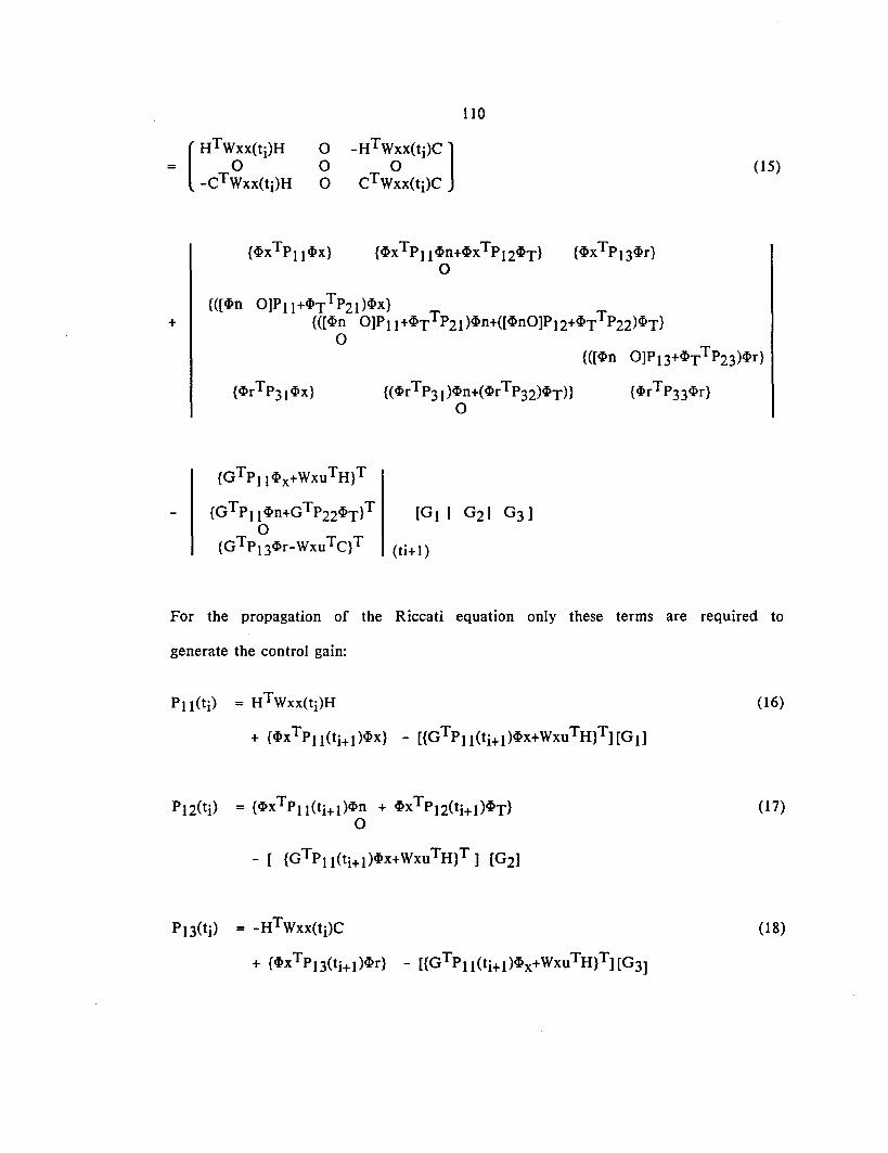
= [HTW~X(ti)H
-cT Wxx(ti)H
110
g -HTW~X(ti)C]
o CTWXX(ti)C(15)
{~xTPll~n+~xTP12~T}o
{([~n O]Pll+~TTP21)~X}+ {([~n O]Pll+~TTP21)~n+{[~nO]P12+~TTP22)~T}
o{([~n O]P13+~TTP23)~r}
{~rTP31~x} {(~rTP31)~n+(~rTP32)~T)} {~rTP33~r}o
{GTPII~x+WXUTH}T
{GTPll~n+GTP22~T}T [GI I G21 G3]o
{GTP13~r-WxuTC}T (ti+l)
For the propagation of the Riccati equation only these terms are required to
generate the control gain:
Pll(ti) = HTWxx(tj)H
+ {~xTPll(ti+I)~X} - [(GTPll(ti+I)~X+WxuTH}T][GIl
PI2(ti) = {~xTPll(ti+I)~n + ~xTP12(ti+l)~T}o
- [ {GTPll(ti+l)~X+WxuTH}T] [G2]
P13(ti) = -HTWxx(ti)C
+ {~xTP13(ti+I)~r} - [{GTPll(ti+l)~x+WxuTH}T][G3]
(16)
(17)
(18)
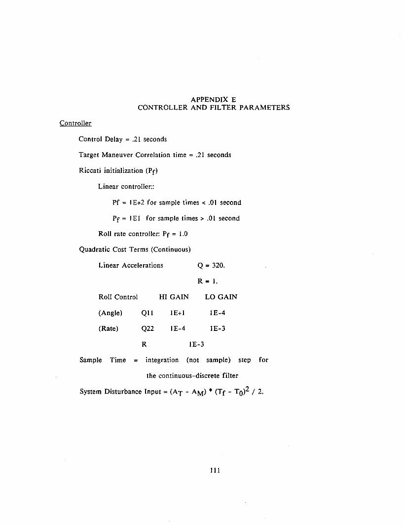
APPENDIX ECONTROLLER AND FILTER PARAMETERS
Controller
Control Delay = .21 seconds
Target Maneuver Correlation time = .21 seconds
Riccati initialization (Pf)
Linear controller::
Pf = IE+2 for sample times < .01 second
Pf = lEI for sample times> .01 second
Roll rate controller: Pf = 1.0
Quadratic Cost Terms (Continuous)
Linear Accelerations Q = 320.
R=l.
Roll Control
(Angle)
(Rate)
QIl
Q22
R
HI GAIN
IE+l
IE-4
lE-3
LO GAIN
lE-4
lE-3
Sample Time = integration (not sample) step for
the continuous-discrete filter
System Disturbance Input = (AT - AM) * (Tf - TO)2 / 2.
III
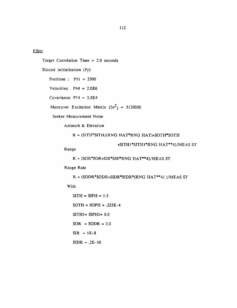
112
Filter
Target Correlation Time = 2.0 seconds
Riccati initialization (Pf)
Positions: PII = 2500
Velocities: P44 = 2.0E6
Covariance: Pl4 = 5.0E4
Maneuver Excitation Matrix (2a2) = 5120000
Seeker Measurement Noise
Azimuth & Elevation
R = (SITH*SITH/(RNG HAT*RNG HAT)+SOTH*SOTH
+SITHI*SITHI*RNG HAT**4)/MEAS STRange
R = (SOR*SOR+SIR*SIR*RNG HAT**4)/MEAS ST
Range Rate
R = (SODR*SODR+SIDR*SIDR*(RNG HAT**4) )/MEAS ST
With
SITH = SIPH = 1.5
SOTH = SOPH = .225E-4
SITHI= SIPHI= 0.0
SOR = SODR = 3.0
SIR = IE-8
SIDR = .2E-IO
LIST OF REFERENCES
[1] A. Arrow, "Status and Concerns for Bank-To-Turn Control of TacticalMissiles," GACIAC PR-85-0 1, "Proceedings of the Workshop on Bank-To-TurnControlled Terminal Homing Missiles," Vol 1, Joint Service Guidance and ControlCommittee, January 1985.
[2] J.R. McClendon and P.L. Verges, "Applications of Modern Control andEstimation Theory to the Guidance and Control of Tactical Air-to-Air Missiles,"Technical Report RG-81-20, "Research on Furure Army Modular Missile," USArmy Missile Command, Redstone Arsenal, Alabama, March 1981.
[3] N.K. Gupta, J.W. Fuller, and T.L. Riggs, "Modern Control Theory Methodsfor Advanced Missile Guidance," Technical Report RG-81-20, "Research onFurure Army Modular Missile," US Army Missile Command, Redstone Arsenal,Alabama, March 1981.
[4] N.B. Nedeljkovic, "New Algorithms for Unconstrained Nonlinear OptimalControl Problems," IEEE Transactions on Automatic Control, Vol. AC-26, No.4,pp 868-884, August 1981.
[5] W.T. Baumann and W.J. Rugh, "Feedback Control of Nonlinear Systems byExtended Linearization," IEEE Transactions on Automatic Control, Vol. AC-31,No.1, pp. 40-46, January 1986.
[6] E.D. Sontag, "Controllability and Linearized Regulation," Department ofMathematics, Rutgers University, New Brunswick, NJ (unpublished), 14 February1097.
[7] A.E. Bryson and Y.C. Ho, Applied Optimal Control, Blaisdell PublishingCompany, Waltham, Massachusetts, 1969.
[8] Y.-S. Lim, "Linearization and Optimization of Stochastic Systems withBounded Control," IEEE Transactions on Automatic Control, Vol. AC-15, No.1,pp 49-52, February 1970.
[9] P.-O. Gutman and P. Hagander, "A New Design of Constrained Controllersfor Linear Systems," IEEE Transactions on Automatic Control, Vol. AC-30, No.1, pp 22-33, January 1985.
[10] R.L. Kousut, "Suboptimal Control of Linear Time-Invariant Systems Subjectto Control Structure Constraints," IEEE Transactions on Automatic Control, Vol.AC-15, No.5, pp 557-562, October 1970.
113
114
[11] D.J. Caughlin, "Bank-To-Turn Control," Master's Thesis, University ofFlorida, 1983.
[12] J.F. Frankena and R. Sivan, "A non-linear optimal control law for linearsystems," INT. J. CONTROL, Vol 30, No I, pp 159-178, 1979.
[13] P.S. Maybeck, Stochastic Models. Estimation. and Control, Volume 3,Academic Press, New York, 1982.
[14] S.A. Murtaugh and H.E. Criel, "Fundamentals of Proportional Navigation,"IEEE Spectrum, pp.75-85, December 1966.
[15] L.A. Stockum, and I.C. Weimer, "Optimal and Suboptimal Guidance for aShort Range Homing Missile," IEEE Trans. on Aerospace and Electronic Systems,Vol. AES-12, No.3, pp 355-361, May 1976.
[16] B. Stridhar, and N.K. Gupta, "Missile Guidance Laws Based on SingularPerturbation Methodology," AIAA Journal of Guidance and Control, Vol 3, No.2,1980.
[17] R.K. Aggarwal and C.R. Moore, "Near-Optimal Guidance Law foraBank-To-Turn Missile," Proceedings 1984 American Control Conference, Volume3, pp. 1408-1415, June 1984.
[18] P.H. Fiske, "Advanced Digital Guidance and Control Concepts forAir-To-Air Tactical Missiles," AFATL-TR-77-130, Air Force ArmamentLaboratory, United States Air Force, Eglin Air Force Base, Florida, January1980.
[19] USAF Test Pilot School, "Stability and Control Flight Test Theory,"AFFTC-77-I, revised February 1977.
[20] L.C. Kramer and M. Athans, "On the Application of DeterministicOptimization Methods to Stochastic Control Problems," IEEE Transactions onAutomatic Control, Vol. AC- 19, No. I, pp 22-30, February 1974.
[21] Y. Bar-Shalom and E. Tse, "Dual Effect, Certainty Equivalence, andSeparation in Stochastic Control," IEEE Transactions on Automatic Control, Vol.AC-19, No.5, pp 494-500, October 1974.
[22] H. Van DE Water and J.C. Willems, "The Certainty Equivalence Property inStochastic Control Theory," IEEE Transactions on Automatic Control, Vol.AC-26, No.5, pp 1080-1086, October 1981.
[23] "Bank-To-Turn Configuration Aerodynamic Analysis Report" RockwellInternational Report No. C77-142Ij034C, date unknown.
115
[24] D.E Williams and B. Friedland, "Design of An Autopilot for Bank-To-TurnHoming Missile Using Modern Control and Estimation Theory," Proc FifthMeeting of the Coordinating Group on Modern Control Theory, 15-27 October1983, (Picatinny) Dover, New Jersey, October 1983, pp. 397-419.
[25] B. Friedland, et aI., "On the "Adiabatic Approximation for Design ofControl Laws for Linear, Time-Varying Systems," IEEE Transactions onAutomatic Control, Vol. AC- 32, No.1, pp. 62-63, January 1987.
[26] D.W. Tufts and D.A. Shnidman, "Optimum Waveforms Subject to BothEnergy and Peak-Value Constraints," Proceedings of the IEEE, September 1964.
[27] M. Pontier and J. Szpirglas, "Linear Stochastic Control with Constraints,IEEE Transactions on Automatic Control, Vol. AC-29, No. 12, pp 1100-1103,December 1984.
[28] P.-O. Gutman and S. Gutman, "A Note on the Control of Uncertain LinearDynamical Systems with Constrained Control Input," IEEE Transactions onAutomatic Control, Vol. AC-30, No.5, pp 484-486, May 1985.
[29] M.W. Spong, J.S. Thorp, and J.M. Kleinwaks, "The Control of RobotManipulators with Bounded Input," IEEE Transactions on Automatic Control, Vol.AC-31, No.6, pp 483-489, June 1986.
[30] D. Feng and B.H. Krogh, "Acceleration-Constrained Time Optimal Controlin n Dimensions," IEEE Transactions on Automatic Control, Vol. AC-31, No. 10,pp 955-958, October 1986.
[31] B.R. Barmish and W.E. Schmitendorf, "New Results on Controllability ofSystems of the Form x(t) = A(t)x(t) + F(t,u(t»," IEEE Transactions onAutomatic Control, Vol. AC-25, No.3, pp 540-547, June 1980.
[32] W.-G. Hwang and W.E. Schmitendorf, "Controllability Results for Systemswith a Nonconvex Target," IEEE Transactions on Automatic Control, Vol. AC-29,No.9, pp 794-802, September 1984.
[33] T. Kaliath, Linear Systems, Prentice-Hall, Inc., Englewood Cliffs, NewJersey, 1980.
[34] M. Vidyasager, Nonlinear Systems Analysis, Prentice-Hall, Englewood Cliffs,New Jersey, 1978.
[35] K. Zhou, and P. Khargonekar, "Stability Robustness Bounds for LinearState-Space Models with Structured Uncertainity," Transactions on AutomaticControl, Vol. AC- 32, No.7, pp 621-623, July 1987.
[36] K.G. Shin and N.D. McKay, "Minimum Time Control of Robotic Manipulatorswith Geometric Path Constraints," IEEE Transactions on Automatic Control, Vol.AC-30, No.6, pp 531-541, June 1985.
116
[37] A. Sabari and H. Khalil. "Stabilization and Regulation of NonlinearSingularly Perturbed Systems Composite Control," IEEE Transactions onAutomatic Control, Vol. AC- 30, No.8, pp. 739-747, August 1985.
[38] M. Sampei and K. Furuta, "On Time Scaling for Nonlinear Systems:Application to Linearization." IEEE Transactions on Automatic Control, Vol.AC-31. No.5, pp 459-462, May 1986.
[39] I.J. Ha and E.G. Gilbert. "A Complete Characterization of DecouplingControl Laws for a General Class of Nonlinear Systems," IEEE Transactions onAutomatic Control, Vol. AC- 31, No.9, pp. 823-830. September 1986.
[40] H. K wakernaak and R. Sivan, Linear Optimal Control Systems,Wiley-Interscience. New York, 1972.
[41] R.A. Singer. "Estimating Optimal Tracking Filter Performance for MannedManeuvering Targets," IEEE Transactions on Aerospace and Electronic Systems,Vol. AES- 6, No.4, pp 473-483, July 1970.
[42] M.E Warren and T.E. Bullock, "Development and Comparison of OptimalFilter Techniques with Application to Air-to-Air Missiles," Electrical EngineeringDepartment. University of Florida, Prepared for the Air Force ArmamentLaboratory, Eglin Air Force Base, Florida, March 1980.
BIOGRAPHICAL SKETCH
Donald J. Caughlin, Jr., was born in San Pedro, California on 17 Dec. 1946.
He graduated from the United States Air Force Academy, earning a B.S. in
physics, and chose pilot training instead of an Atomic Energy Commission
Fellowship. Since then he has flown over 3100 hours in over 60 different
aircraft and completed one tour in Southeast Asia flying the A-I Skyraider. A
Distinguished Graduate of the United States Air Force Test Pilot School, Don
has spent much of his career in research, development, and test at both major
test facilities--Eglin AFB in Florida, and Edwards AFB in California.
Don Caughlin is a Lieutenant Colonel in the United States Air Force cur
rently assigned as the Assistant for Senior Officer Management at Headquarters
Air Force Systems Command.
In addition to the B.S. in physics, Lt. Colonel Caughlin has an M.B.A. from
the University of Utah, and a masters degree in electrical engineering from the
University of Florida. He is a member of the Society of Experimental Test
Pilots and IEEE.
Lt. Colonel Caughlin is married to the former Barbara Schultz of
Montgomery, Alabama. They have two children, a daughter, Amy Marie, age
eight, and Jon Andrew, age four.
117
AUTHOR:TITLE:
Internet Distribution Consent AgreementIn reference to the following dissertation:
Caughlin, DonaldReachable Set Control for Preferred Axis Homing Missles (recordnumber: 1102747)
PUBLICATION DATE: 1988
I, fiJ oJ ~/,{t as copyright holder for theaforementioned dissertation, hereby grant specific and limited archive and distribution rights tothe Board of Trustees of the University of Florida and its agents. I authorize the University ofFlorida to digitize and distribute the dissertation described above for nonprofit, educationalpurposes via the Internet or successive technologies.
This is a non-exclusive grant of permissions for specific off-line and on-line uses for anindefinite term. Off-line uses shall be limited to those specifically allowed by "Fair Use" asprescribed by the terms of United States copyright legislation (cf, Title 17, U.S. Code) as well asto the maintenance and preservation of a digital archive copy. DigbiMliM allows the Universityof Florida to generate image- and text-based versions as appropriate.and.to,provide and enhanceaccess using search software.
rohibits use of the digitim4 versivns w~ommelcial use or profit.
personal information blurred
Date of Signature
Please print, sign and return to:Cathleen Martyniak
UF Dissertation ProjectPreservation Department
University of Florida LibrariesP.O. Box 117007
Gainesville, FL 32611-7007
512812008