2 Published by the IEEE CS and AIP 1521-9615/03/$17.00 © 2003 IEEE COMPUTING IN SCIENCE & ENGINEERING

Editors: Isabel Beichl, isabel.beichl@nist.gov

Julian V. Noble, jvn@virginia.edu

PRESCRIPTIONSC O M P U T I N G P R E S C R I P T I O N S

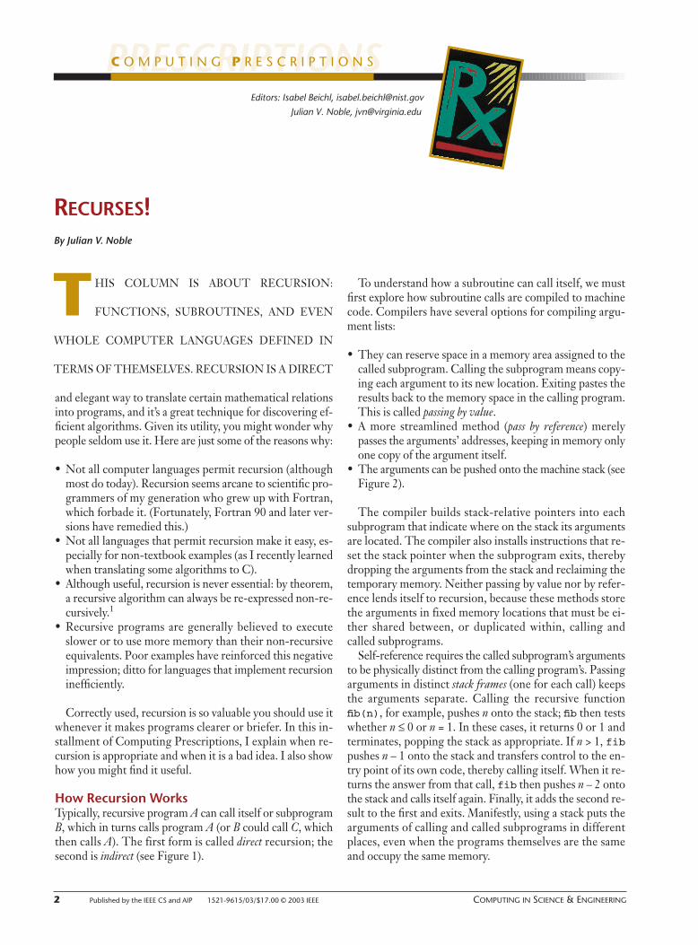
and elegant way to translate certain mathematical relationsinto programs, and it’s a great technique for discovering ef-ficient algorithms. Given its utility, you might wonder whypeople seldom use it. Here are just some of the reasons why:

• Not all computer languages permit recursion (althoughmost do today). Recursion seems arcane to scientific pro-grammers of my generation who grew up with Fortran,which forbade it. (Fortunately, Fortran 90 and later ver-sions have remedied this.)

• Not all languages that permit recursion make it easy, es-pecially for non-textbook examples (as I recently learnedwhen translating some algorithms to C).

• Although useful, recursion is never essential: by theorem,a recursive algorithm can always be re-expressed non-re-cursively.1

• Recursive programs are generally believed to executeslower or to use more memory than their non-recursiveequivalents. Poor examples have reinforced this negativeimpression; ditto for languages that implement recursioninefficiently.

Correctly used, recursion is so valuable you should use itwhenever it makes programs clearer or briefer. In this in-stallment of Computing Prescriptions, I explain when re-cursion is appropriate and when it is a bad idea. I also showhow you might find it useful.

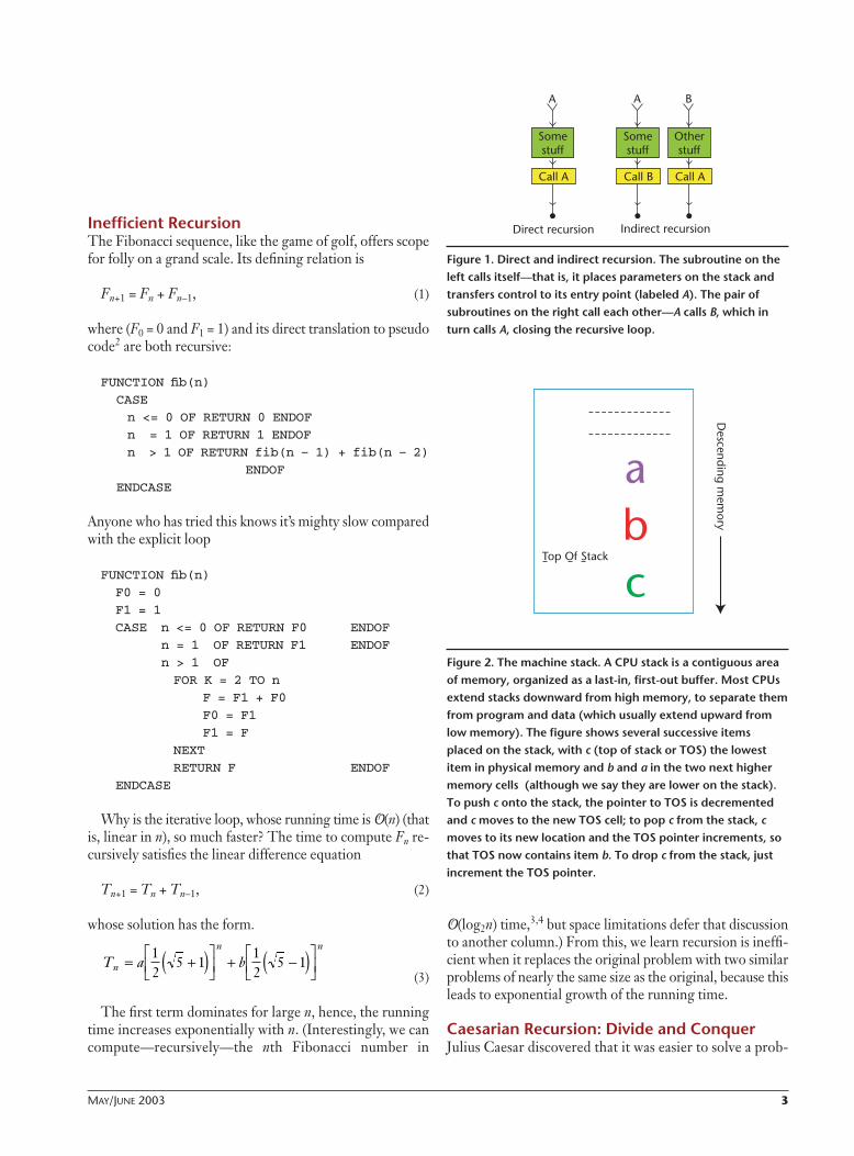
How Recursion WorksTypically, recursive program A can call itself or subprogramB, which in turns calls program A (or B could call C, whichthen calls A). The first form is called direct recursion; thesecond is indirect (see Figure 1).

To understand how a subroutine can call itself, we mustfirst explore how subroutine calls are compiled to machinecode. Compilers have several options for compiling argu-ment lists:

• They can reserve space in a memory area assigned to thecalled subprogram. Calling the subprogram means copy-ing each argument to its new location. Exiting pastes theresults back to the memory space in the calling program.This is called passing by value.

• A more streamlined method (pass by reference) merelypasses the arguments’ addresses, keeping in memory onlyone copy of the argument itself.

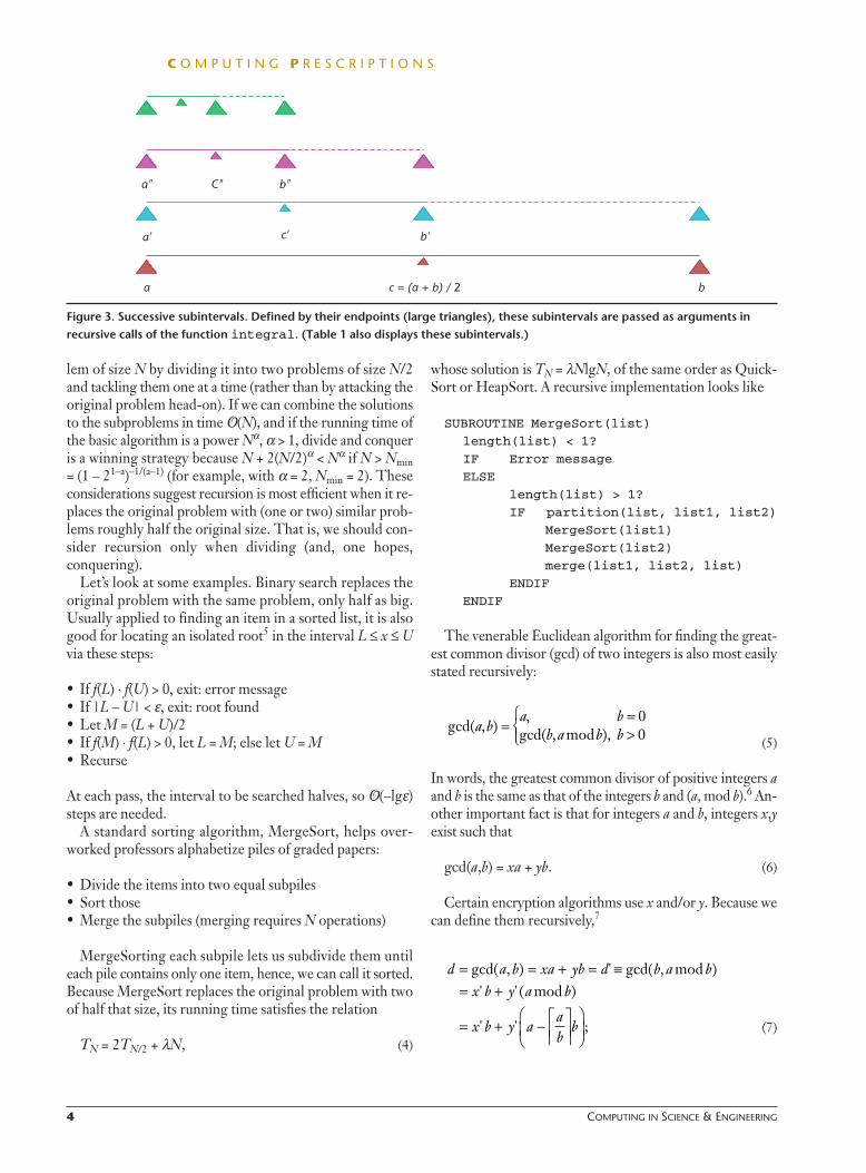
• The arguments can be pushed onto the machine stack (seeFigure 2).

The compiler builds stack-relative pointers into eachsubprogram that indicate where on the stack its argumentsare located. The compiler also installs instructions that re-set the stack pointer when the subprogram exits, therebydropping the arguments from the stack and reclaiming thetemporary memory. Neither passing by value nor by refer-ence lends itself to recursion, because these methods storethe arguments in fixed memory locations that must be ei-ther shared between, or duplicated within, calling andcalled subprograms.

Self-reference requires the called subprogram’s argumentsto be physically distinct from the calling program’s. Passingarguments in distinct stack frames (one for each call) keepsthe arguments separate. Calling the recursive functionfib(n), for example, pushes n onto the stack; fib then testswhether n ≤ 0 or n = 1. In these cases, it returns 0 or 1 andterminates, popping the stack as appropriate. If n > 1, fibpushes n – 1 onto the stack and transfers control to the en-try point of its own code, thereby calling itself. When it re-turns the answer from that call, fib then pushes n – 2 ontothe stack and calls itself again. Finally, it adds the second re-sult to the first and exits. Manifestly, using a stack puts thearguments of calling and called subprograms in differentplaces, even when the programs themselves are the sameand occupy the same memory.

RECURSES!By Julian V. Noble

T HIS COLUMN IS ABOUT RECURSION:

FUNCTIONS, SUBROUTINES, AND EVEN

WHOLE COMPUTER LANGUAGES DEFINED IN

TERMS OF THEMSELVES. RECURSION IS A DIRECT

MAY/JUNE 2003 3

Inefficient RecursionThe Fibonacci sequence, like the game of golf, offers scopefor folly on a grand scale. Its defining relation is

Fn+1 = Fn + Fn–1, (1)

where (F0 = 0 and F1 = 1) and its direct translation to pseudocode2 are both recursive:

FUNCTION fib(n)

CASE

n <= 0 OF RETURN 0 ENDOF

n = 1 OF RETURN 1 ENDOF

n > 1 OF RETURN fib(n – 1) + fib(n – 2)

ENDOF

ENDCASE

Anyone who has tried this knows it’s mighty slow comparedwith the explicit loop

FUNCTION fib(n)

F0 = 0

F1 = 1

CASE n <= 0 OF RETURN F0 ENDOF

n = 1 OF RETURN F1 ENDOF

n > 1 OF

FOR K = 2 TO n

F = F1 + F0

F0 = F1

F1 = F

NEXT

RETURN F ENDOF

ENDCASE

Why is the iterative loop, whose running time is O(n) (thatis, linear in n), so much faster? The time to compute Fn re-cursively satisfies the linear difference equation

Tn+1 = Tn + Tn–1, (2)

whose solution has the form.

(3)

The first term dominates for large n, hence, the runningtime increases exponentially with n. (Interestingly, we cancompute—recursively—the nth Fibonacci number in

O(log2n) time,3,4 but space limitations defer that discussionto another column.) From this, we learn recursion is ineffi-cient when it replaces the original problem with two similarproblems of nearly the same size as the original, because thisleads to exponential growth of the running time.

Caesarian Recursion: Divide and ConquerJulius Caesar discovered that it was easier to solve a prob-

T a bn

n n

= +( )

+ −( )

12

5 112

5 1

Direct recursion

Somestuff

Call A

A

Somestuff

Call B

A

Otherstuff

Call A

B

Indirect recursion

Figure 1. Direct and indirect recursion. The subroutine on theleft calls itself—that is, it places parameters on the stack andtransfers control to its entry point (labeled A). The pair ofsubroutines on the right call each other—A calls B, which inturn calls A, closing the recursive loop.

Descending m

emory

Top Of Stack

Figure 2. The machine stack. A CPU stack is a contiguous areaof memory, organized as a last-in, first-out buffer. Most CPUsextend stacks downward from high memory, to separate themfrom program and data (which usually extend upward fromlow memory). The figure shows several successive itemsplaced on the stack, with c (top of stack or TOS) the lowestitem in physical memory and b and a in the two next highermemory cells (although we say they are lower on the stack).To push c onto the stack, the pointer to TOS is decrementedand c moves to the new TOS cell; to pop c from the stack, cmoves to its new location and the TOS pointer increments, sothat TOS now contains item b. To drop c from the stack, justincrement the TOS pointer.

4 COMPUTING IN SCIENCE & ENGINEERING

lem of size N by dividing it into two problems of size N/2and tackling them one at a time (rather than by attacking theoriginal problem head-on). If we can combine the solutionsto the subproblems in time O(N), and if the running time ofthe basic algorithm is a power Nα, α > 1, divide and conqueris a winning strategy because N + 2(N/2)α < Nα if N > Nmin= (1 – 21–a)–1/(a–1) (for example, with α = 2, Nmin = 2). Theseconsiderations suggest recursion is most efficient when it re-places the original problem with (one or two) similar prob-lems roughly half the original size. That is, we should con-sider recursion only when dividing (and, one hopes,conquering).

Let’s look at some examples. Binary search replaces theoriginal problem with the same problem, only half as big.Usually applied to finding an item in a sorted list, it is alsogood for locating an isolated root5 in the interval L ≤ x ≤ Uvia these steps:

• If f(L) ⋅ f(U) > 0, exit: error message• If |L – U| < ε, exit: root found• Let M = (L + U)/2• If f(M) ⋅ f(L) > 0, let L = M; else let U = M• Recurse

At each pass, the interval to be searched halves, so O(–lgε)steps are needed.

A standard sorting algorithm, MergeSort, helps over-worked professors alphabetize piles of graded papers:

• Divide the items into two equal subpiles• Sort those• Merge the subpiles (merging requires N operations)

MergeSorting each subpile lets us subdivide them untileach pile contains only one item, hence, we can call it sorted.Because MergeSort replaces the original problem with twoof half that size, its running time satisfies the relation

TN = 2TN/2 + λN, (4)

whose solution is TN = λNlgN, of the same order as Quick-Sort or HeapSort. A recursive implementation looks like

SUBROUTINE MergeSort(list)

length(list) < 1?

IF Error message

ELSE

length(list) > 1?

IF partition(list, list1, list2)

MergeSort(list1)

MergeSort(list2)

merge(list1, list2, list)

ENDIF

ENDIF

The venerable Euclidean algorithm for finding the great-est common divisor (gcd) of two integers is also most easilystated recursively:

(5)

In words, the greatest common divisor of positive integers aand b is the same as that of the integers b and (a, mod b).6 An-other important fact is that for integers a and b, integers x,yexist such that

gcd(a,b) = xa + yb. (6)

Certain encryption algorithms use x and/or y. Because wecan define them recursively,7

(7)

d a b xa yb d b a bx b y a b

x b y aab

b

= = + = ≡= +

= + −

gcd( , ) ' gcd( , mod )' '( mod )

' ' ;

gcd( , )

,gcd( , mod ),a ba b

b a b b==>

00

C O M P U T I N G P R E S C R I P T I O N S

a" C" b"

a' c' b'

a c = (a + b) / 2 b

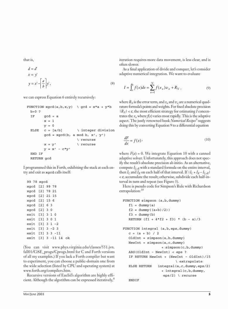
Figure 3. Successive subintervals. Defined by their endpoints (large triangles), these subintervals are passed as arguments inrecursive calls of the function integral. (Table 1 also displays these subintervals.)

MAY/JUNE 2003 5

that is,

(8)

we can express Equation 6 entirely recursively:

FUNCTION xgcd(a,b,x,y) \ gcd = x*a + y*b

b=0 ?

IF gcd = a

x = 1

y = 0

ELSE c = [a/b] \ integer division

gcd = xgcd(b, a mod b, x’, y’)

\ recurse

x = y’ \ recurse

y = x’ - c*y’

END IF

RETURN gcd

I programmed this in Forth, exhibiting the stack at each en-try and exit as xgcd calls itself:

99 78 xgcd

xgcd [2] 99 78

xgcd [2] 78 21

xgcd [2] 21 15

xgcd [2] 15 6

xgcd [2] 6 3

xgcd [2] 3 0

exit [3] 3 1 0

exit [3] 3 0 1

exit [3] 3 1 -2

exit [3] 3 -2 3

exit [3] 3 3 -11

exit [3] 3 -11 14 ok

(You can visit www.phys.virginia.edu/classes/551.jvn.fall01/CiSE_progs/Cprogs.html for C and Forth versionsof all my examples.) If you lack a Forth compiler but wantto experiment, you can choose a public-domain one fromthe wide selection (listed by CPU and operating system) atwww.forth.org/compilers.htm.

Recursive versions of Euclid’s algorithm are highly effi-cient. Although the algorithm can be expressed iteratively,8

iteration requires more data movement, is less clear, and isoften slower.

As a final application of divide and conquer, let’s consideradaptive numerical integration. We want to evaluate

, (9)

where RN is the error term, and xn and wn are a numerical quad-rature formula’s points and weights. For fixed absolute precision|RN| < ε, the most efficient strategy for estimating I concen-trates the xn where f(x) varies most rapidly. This is the adaptiveaspect. The justly renowned book Numerical Recipes9 suggestsdoing this by converting Equation 9 to a differential equation

, (10)

where F(a) = 0. We integrate Equation 10 with a cannedadaptive solver. Unfortunately, this approach does not spec-ify the result’s absolute precision ab initio. As an alternative,compute IL+R with a standard formula on the entire interval,then IL and IR on each half of that interval. If |IL + IR – IL+R|< ε, accumulate the result; otherwise, subdivide each half-in-terval in turn and repeat (see Figure 3).

Here is pseudo code for Simpson’s Rule with Richardsonextrapolation:10

FUNCTION simpson (a,b,dummy)

f1 = dummy(a)

f2 = dummy((a+b)/2))

f3 = dummy(b)

RETURN (f1 + 4*f2 + f3) * (b - a)/3

FUNCTION integral (a,b,eps,dummy)

c = (a + b) / 2

OldInt = simpson(a,b,dummy)

NewInt = simpson(a,c,dummy)

+ simpson(c,b,dummy)

ABS(OldInt - NewInt) < eps ?

IF RETURN NewInt + (NewInt - OldInt)/15

\ extrapolate

ELSE RETURN integral(a,c,dummy,eps/2)

+ integral(c,b,dummy,

eps/2) \ recurse

ENDIF

dFdx

f x= ( )

I f x dx f x w Rn n N

n

N

a

b= = +

=∑∫ ( ) ( )

1

d dx y

y xab

y

==

= −

''

' ' ,

6 COMPUTING IN SCIENCE & ENGINEERING

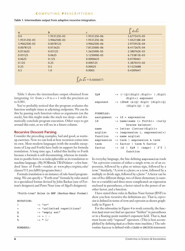
Table 1 shows the intermediate output obtained fromintegrating from x = 0 to x = 1 with the precision setto 0.001.

You’ve probably noticed that the program evaluates thefunction multiple times at adjoining endpoints. We can fixthis by passing such function values as arguments (on thestack), but this might make the stack too deep—and dra-matically conclude program execution. Other ways to getaround this exist, as we will see in a future column.

Recursive Descent ParsingConsider the preceding examples, bad and good, as warm-up exercises. Now we can look at how recursion comes intoits own. Most modern languages (with the notable excep-tions of Lisp and Forth) have built-in support for formulatranslation. A long time ago, I added this facility to Forthbecause a formula is self-documenting, whereas its transla-tion to postfix form is as indecipherable as its translation tomachine language. (My FORmula TRANslator—a few hun-dred lines of Forth—resides at www.phys.virginia.edu/classes/551.jvn.fall01/programs.htm.)

Formula translation is an instance of rule-based program-ming. We can specify a “Forth-tran” formula by rules statedin a specialized format devised by John Backus (one of For-tran’s designers) and Peter Naur (one of Algol’s designers):

“Forth-tran” Rules in BNF (Backus-Naur Format)

NOTATION:

| -> “or”

+ -> “unlimited repetitions”

Q -> “empty set”

& -> + | -

% -> * 1/

NUMBERS:

fp# -> {-|Q}{digit.digit+ |.digit

digit+} exponent

exponent -> {dDeE {&|Q} digit {digit|Q}

{digit|Q} | Q}

FORMULAS:

assignment -> id = expression

id -> name|name {+ Forth}+ –curly

braces balance!

name -> letter {letter|digit}+

arglist -> (expression {, expression}+)

function -> name arglist

expression -> term | expression & term

term -> factor | term % factor

factor -> id | fp# | (expr) | f∧f |

function

In everyday language, the line defining expression reads“An expression consists of either a single term; or of an ex-pression, followed by a plus or minus sign, followed by aterm.” Similarly, “A term is a factor; or a term, followed by amultiply or divide sign, followed by a factor.” A factor can beone of five different things, two of them elementary (a num-ber or a variable) and three more complicated: an expressionenclosed in parentheses, a factor raised to the power of an-other factor, and a function.

I have stated these rules in Backus-Naur format (BNF) toshow you how recursive the definitions are. That is, expres-sion is defined in terms of term and expression as shown graph-ically in Figure 4.

For the subroutine in Figure 4 to work correctly, the func-tion find must not find an operator “hidden” in parenthesesor in a floating-point number’s exponent field. That is, findmust locate only “exposed” operators. (This is best accom-plished by defining find as a finite-state machine.) The sub-routine factor is defined with a CASE or SWITCH statement:

x

C O M P U T I N G P R E S C R I P T I O N S

Table 1. Intermediate output from adaptive recursive integration.

a b ε0.0 1.953125E–03 1.953125E–06 5.677541E–051.953125E–03 3.906250E–03 1.953125E–06 1.052158E–043.906250E–03 0.0078125 3.906250E–06 2.975953E–040.0078125 0.015625 7.812500E–06 8.417267E–040.015625 0.03125 1.562500E–05 2.380762E–030.03125 0.0625 3.125000E–05 6.733813E–030.0625 0.125 0.0000625 0.01904610.125 0.25 0.000125 5.387051E–020.25 0.5 0.00025 0.15236880.5 1.0 0.0005 0.4309641

dx x = 0.66666530

1∫

dx xa

b∫

MAY/JUNE 2003 7

SUBROUTINE factor(beg, end)

CASE

id OF do_id(beg, end) ENDOF

fp# OF do_fp(beg, end) ENDOF

f∧f OF do_power(beg, end) ENDOF

(expr) OF expression(beg+1, end-1)

ENDOF

function OF do_funct(beg, end) ENDOF

END CASE

We can write the entire program recursively like this so thatit generates the appropriate output from the input text. Noteespecially that because term calls factor, which then callsexpression, the recursion is indirect but mirrors the rulesprecisely.

Symbolic manipulationBecause I plan to discuss computer algebra in a future col-umn, I won’t dwell on it here. An algebra program uses thesame principles as a compiler: it translates statements in onelanguage to another, perhaps performing manipulations dur-ing the process. The key again is to work out the rules andimplement them. For example, the rules for differentiatinga function are

diff [αf(x) + βg(x)] = α diff [f(x)] + β diff [g(x)]diff [f(x) ⋅ g(x)] = g(x) diff f(x) + f(x) diff g(x)diff f(g(x)) = diff g(x) diff f(g), (11)

to which we add a library of derivatives of known functions.Many algebraic operations (such as differentiation) are innatelyrecursive, hence, we can translate them directly to a recursiveprogram. I’ll also defer those details to a future column.

I hope these illustrations have shown you some of thepower and elegance of recursion. To see the difference

between recursive and iterative versions of several codes,please check my Web site. Expect lots more recursive appli-cations in future articles.

References1. R.L. Kruse, Data Structures and Program Design, 2nd ed., Prentice-Hall,

1987.

2. B. Einarsson and Y. Shokin, Fortran 90 for the Fortran 77 Programmer,version 2.3, 1996, www.nsc.liu.se/~boein/f77to90.

3. E.B. Escott, “Procédé Expéditif pour Calculer un Terme très Éloigné dansla Série de Fibonacci” (“Fast Algorithm for Calculating Remote Terms in

the Fibonacci Series”), L’Intermédiaire des Mathématiciens (Mathemati-cian’s J.), vol. 7, 1900, pp. 172–175.

4. J.C.P. Miller and D.J. Spencer Brown, “An Algorithm for Evaluation ofRemote Terms in a Linear Recurrence Sequence,” Computer J., vol. 9,1966, pp. 188–190.

5. F.S. Acton, Numerical Methods that Work, Mathematical Assoc. America,1990, p. 179.

6. G. Birkhoff and S. MacLane, A Survey of Modern Algebra, 5th ed., A.K.Peters Ltd., 1996.

7. T.H. Cormen, C.E. Leiserson, and R.L. Rivest, Introduction to Algorithms,MIT Press, 1990.

8. D.E. Knuth, The Art of Computer Programming, 3rd ed., Addison WesleyLongman, 1997, p. 13ff.

9. W.H. Press et al., Numerical Recipes: The Art of Scientific Computing, Cam-bridge Univ. Press, 1986.

10. A. Ralston, A First Course in Numerical Analysis, McGraw-Hill, 1965, p.118ff.

Julian Noble is a physics professor at the University of Virginia. His in-

terests are eclectic, both in and out of physics. His teaching philosophy

is “no black boxes.” Contact him at the Dept. of Physics, Univ. of Vir-

ginia, PO Box 400714, Charlottesville, VA 22904-4714; jvn@virginia.edu.

Expression

Find + or -

Found?

No

Term Expression

Term

Yes

Figure 4. A graphic representation of pseudo code for thesubroutine expression. Starting from the right end of thestring, expression looks for an exposed + or – sign. If itfinds one, it breaks the string there and treats it as anexpression plus a term; if it finds no exposed sign, it treats thewhole string as a term. Thus it embodies both direct recursion(when expression calls itself), and indirect recursion (whenexpression calls term).