Embed Size (px)
Citation preview
RDFMatView: Indexing RDF Data for SPARQLQueries
Roger Castillo, Christian Rothe, and Ulf Leser
Humboldt Universtiy of Berlin{castillo,rothe,leser}@informatik.hu-berlin.de
http://www.hu-berlin.de/
Abstract. The Semantic Web as an evolution of the World Wide Web aims tocreate a universal medium for the exchange of semantically described data. Theidea of representing this information by means of directed labelled graphs, RDF,has been widely accepted by the scientific community. However querying RDFdata sets to find the desired information often is highly time consuming due tothe number of comparisons that are needed. In this article we propose indexeson RDF to reduce the search space and the SPARQL query processing time. Ourapproach is based on materialized queries, i.e., precomputed query patterns andtheir occurrences in the data sets. We provide a formal definition of RDFMatViewindexes for SPARQL queries, a cost model to evaluate their potential impact onquery performance, and a rewriting algorithm to use indexes in SPARQL queries.We also develop and compare different approaches to integrate such indexes intoan existing SPARQL query engine. Our preliminary results show that our ap-proach can drastically decrease the query processing time in comparison to con-ventional query processing.
Key words: SPARQL, Indexing, RDF, Materialized views
2 Roger Castillo, Christian Rothe, and Ulf Leser
1 Introduction
The Semantic Web as an evolution of the World Wide Web is an important initiativewhich has recently gained momentum. It aims to create a universal medium for the ex-change of data where data can be shared and processed by automated tools as well as bypeople. The basis for this proposal is a logical data model called Resource DescriptionFramework (RDF) [1]. An RDF data set is a collection of statements called triples, ofthe form (s,p,o) where s is a subject, p is a predicate and o is an object. Each triplestates the relation between subject and object. A set of triples can be represented asa directed graph where subjects and objects represent nodes and predicates representedges connecting these nodes. The SPARQL query language is the official standard forsearching over RDF repositories [2]. It supports operations of triple patterns, similarto select-project-join queries in relational databases. For instance, using the SPARQLquery in Listing 1 we can retrieve articles written by Albert Einstein from a local RDFdata store.
SELECT ? t i t l e WHERE {? a r t i c l e <h a s T i t l e > ? t i t l e .? a r t i c l e <hasAuthor > ? a u t h o r .? a u t h o r <hasName> ” A l b e r t E i n s t e i n ” .}
Listing 1. SPARQL query to retrieve all articles written by Albert Einstein
Listing 1 illustrates a simple SPARQL query where each join is denoted by a dot. Thewhole query pattern can be seen as a graph pattern that needs to be matched in the RDFdata set. Predicates may also contain, which increases the complexity of query evalua-tion.
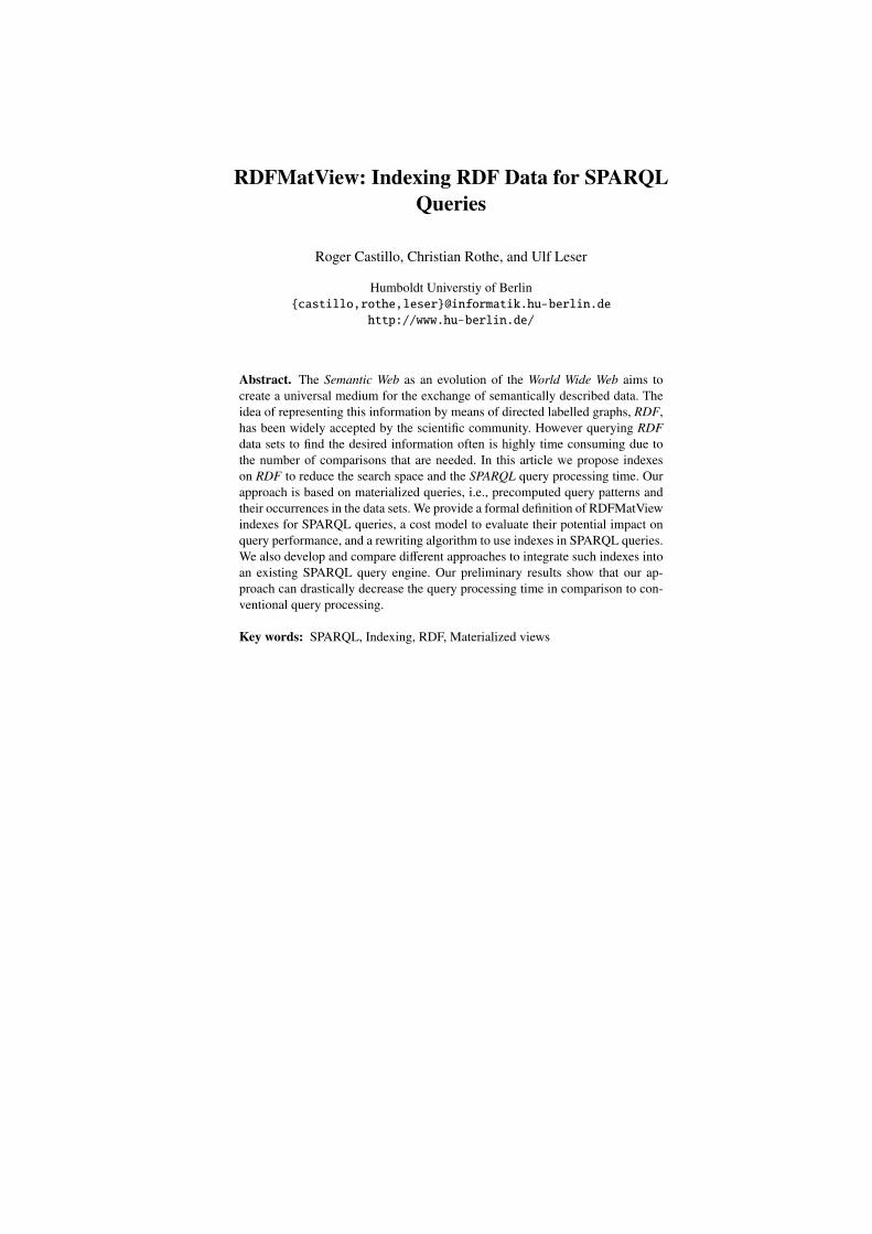
The increasing amount of RDF data on the Web requires the development of ap-proaches for efficient RDF data management. Almost all recent implementations ofSPARQL are build upon relational databases (e.g. Jena [3], 3Store [4, 5], or Sesame[6]). In these systems, a SPARQL query is translated into one or more SQL queriesover a relational representation of the underlying RDF data set. This relational repre-sentation usually stores RDF triples in one or a few tables. Consequently, answering aSPARQL query consisting of more than one pattern requires the computation of roughlyas many joins as the query has patterns. Optimizing these joins is one of the critical is-sues to obtain scalable SPARQL systems.The typical architecture used by these approaches is shown in Figure 1. This architec-ture is based on a 3-Layer schema which consists of the SPARQL query interface, theRDF data representation and the underlying database.
In this work, we propose the use of materialized SPARQL queries to speed-upqueries. We target large data sets and SPARQL queries consisting of many basic graphpatterns. Examples of huge data sets are, for instance, the UniProt database containingmore than 600 million triples [7] or the W3C SWEO Linking Open Data Communitywith more than 4 billion triples [8]. With such datasets, executing a query with manygraph patterns becomes a problem.
RDFMatView: Indexing RDF Data for SPARQL Queries 3
Fig. 1. SPARQL Query Processing using a typical RDBMS - Backend Architecture.
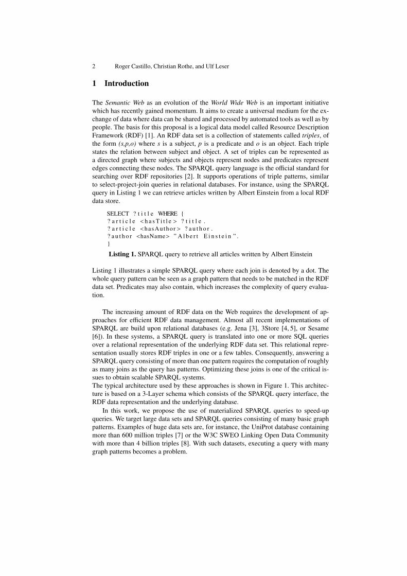
SELECT ∗ WHERE {? s1 ? p1 ? o1 .? o1 b i f : c o n t a i n s ” h e x o k i n a s e ” .? s1 < type > ? t y p e 1 .? s1 <comment> ? comment1 .? s1 < l a b e l > ? l a b e l 1 .? s1 <isA> ? s2 .? s2 <comment> ? comment2 .? s2 < l a b e l > ? l a b e l 2 . }
Listing 2. Example SPARQL query. Information about Hexokinase enzyme [9]
Consider the query given in Listing 2, which a real-life query taken from [9] gath-ering information about a certain enzyme from a database. Executing this query on aconventional SPARQL processor will result in the computation of seven-way self-joinof the triple table. However, one can safely assume that the types, labels, and commentsof an object are used together very often. Therefore, we suggest to materialize this in-formation by executing a query off-line and storing the results inside the system. Giventhis materialized query, the query could be computed with only four joins.
In contrary to previous approaches which focus on indexing the relational represen-tation of an RDF storage scheme, we fully exploit the RDF graph-structure for indexing.We are not indexing single attributes or triples, but fractions of queries that occur fre-quently in an expected workload. Therefore, our approach is a native RDF/SPARQLindexing method whose concepts are viable for all possible implementations of RDFstores. Such an approach requires solutions to a whole series of problems. First, querieshave to be materialized. Second, the query must be analyzed to identify all material-ized queries that could be used, and especially to identify the best such query or bestcombination of such queries that should be used. This requires complex query planningalgorithms and a cost model. Third, the query processing itself must be modified to be
4 Roger Castillo, Christian Rothe, and Ulf Leser
able to retrieve materialized results and to combine them with those parts of the originalquery that are not covered by the indexes.
More formally, this paper presents solutions to the following problems.
– Generation of execution plans to cover a query. Given a query Q for a data graph Gand the set I of all indexes on G, the first step is to define which indexes are usablefor speeding up Q. To this end, we need to generate all possible mappings betweenthe index pattern and the query.
– Definition of a cost model to assess different query execution plans. Each plan dif-fers from the others according to the parts of the query that are covered by indexes,which in turn leads to different sizes of intermediate results and different parts ofthe query that need to be executed and combined with the materialized parts. Theobjective of the cost model is to assess all possible plans and to find those withminimal estimated cost.
– Rewriting of a SPARQL query to substitute covered query patterns by RDFMatViewindexes. When a combination of RDFMatView indexes is selected, its materializedresults must combined to occurrences of the covered query pattern. There are twodifferent cases how this may happen:1. The combination of indexes completely cover the query pattern. Thus, the so-
lution to the query can be generated completely by joining the indexes.2. The combination of indexes only partially cover the query pattern. Then, the
query solution needs to be generated by joining the results of the chosen in-dexes with the residual parts of the query pattern.
In this report, we present solutions to all of these problems. We first discuss relatedwork in Section 2. Section 3 introduces basic concepts of RDF and SPARQL. Section4 presents the fundamental principles of RDFMatViews and a strategy to use them forSPARQL query processing. Section 5 introduces the cost model used to evaluate dif-ferent query plans. We describe different ways to introduce materialized queries intoan existing SPARQL processor in 6. Finally, we give an evaluation of our method inSection 7 and conclude in Section 8.
We presented a theoretical framework for using materialized SPARQL queries asindexes in [10]. In the present work, we show the practical applicability of this frame-work by describing and comparing several ways to integrate materialized views into anexisting SPARQL query processor and by providing an evaluation on the speed-ups thatcan be achieved using our methods.
Clearly, in a setting such as ours it is also important to provide algorithms to keepmaterialized queries up-to-date, and to give a user hints on which queries should bematerialized to best (best in terms of space/cost-efficiency) support a given workload.However, these questions are out-of-scope of our current research.
RDFMatView: Indexing RDF Data for SPARQL Queries 5
2 Related work
In this section, we discuss published techniques for indexing SPARQL queries andcontrast them to our work.
Most works focus on optimizing a single join. In [11] Abadi et al. propose a verticalpartition approach for Semantic Web data management. An enhancement of this ap-proach is proposed by Weiss et al. in [12]. Therein, RDF data is indexed in six possibleways, i.e., an index for each possible ordering of the three RDF elements. Each instanceof an RDF element is associated with two vectors; each such vector gathers elements ofone of the other types, along with lists of the third-type resources attached to each vectorelement. This scheme is capable of speeding up single joins tremendously, but storagerequirements are very high, which becomes a serious issue when using huge data sets.Neumann and Weikum developed RDF-3X, a SPARQL engine implementation pursu-ing a RISC-style architecture – a streamlined architecture – with specific-designed datastructures and operations [13]. The authors overcome the “giant-triples-table” [11] bot-tleneck by creating a set of indexes and a fast way pf processing merge joins. Similar to[12], RDF-3X maintains all six possible permutations of subject, predicate and objectin six separate indexes. The authors also present a compression algorithm to alleviatethe problem of space consumption.
All these approaches have in common that they focus on single joins. When facedwith queries consisting of multiple basic graph patterns, they still have to computemultiple joins (although every single join is faster). In contrast, our work specificallytargets the speed-up of complex queries consisting of many basic graph patterns.
There is also some other work that considers groups of patterns. In [14] the authorspresent GRIN, a lightweight indexing mechanism for RDF data. The main idea is todraw circles around selected center vertices in the graph where the circle would com-prise those vertices in the graph that are within a given distance of the “center” vertex.Basically, GRIN is a binary tree where the set of leaf nodes form a partition of the setof triples in the RDF graph. An interior node implicitly represents the set of all verticesin the RDF graph that are within a specific unit of distance. To evaluate a query, GRINderives a set of inequality constraints from the query. These constraints are evaluatedagainst the nodes of the GRIN index. A similar indexing approach is presented in [15].This work proposes to create a set of indexes of precomputed joins using all possiblejoin combinations between triple patterns. As [14], this approach aims to create a gen-eral purpose set of indexes based on joined triple patterns, but the number of indexes tomanage is not practical when the number of joined triples is >= 3.
The two systems just described index groups of and not just single triples. How-ever, they propose to apply their techniques to all RDF triples, while we only builduser-chosen indexes. Our work fundamentally is based on the assumption that somepatterns are used together in queries more frequently than others, and that indexingthose combinations suffices to gain large speed-ups at manageable space and mainte-nance cost.
One can best describe the differences between our ideas and that of other RDFindexing schemes by drawing a parallel to B*-indexes in relational databases [16]. No-body would sensibly suggest to speed up queries by indexing every attribute; instead,systems assume that developers have a rough idea about the types of queries that need

6 Roger Castillo, Christian Rothe, and Ulf Leser
to be answered and therefore index only the relevant attributes. Furthermore, optimalspeed-up can only be achieved when also combinations of attributes can be indexed,and not only single attributes. In this sense, the former approaches index every singleattribute, the latter indexes every possible combination of attributes, and we suggest toindex only selected combinations of attributes.
RDFMatView: Indexing RDF Data for SPARQL Queries 7
3 Preliminaries: RDF and SparQL
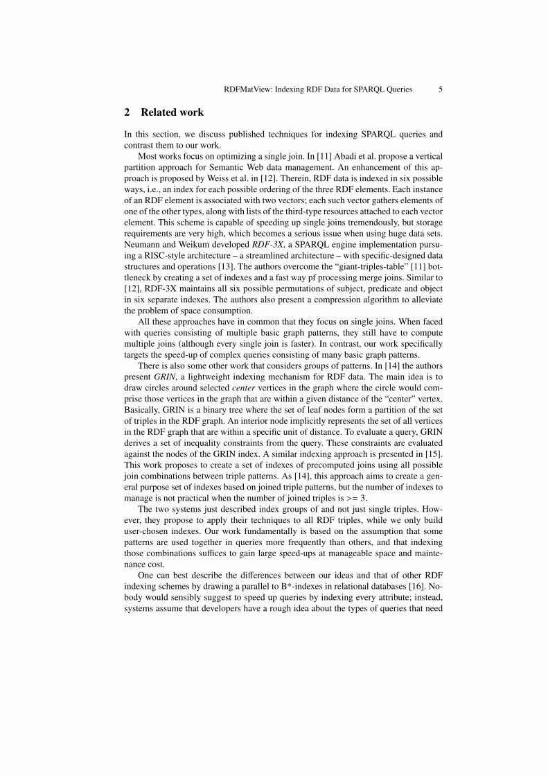
The SparQL query language has increased its popularity since it recently reached acandidate recommendation of the W3C [2] for retrieving information from RDF [1]graphs stored in semantic storage systems. We make the assumption that our audienceis familiar with RDF and SparQL. Thus, we only describe the most important termsfrom this specification which are required for our project. For formal definition of theseconcepts we refer the reader to the RDF specification [1].An RDF graph is a set of RDF Triples, which in turn consist of RDF Terms. An RDFTerm consists of an IRI,1 blank node or an RDF Literal. The set of all RDF terms isdenoted in this article as RDF-T. The building blocks of a SparQL query are triplepatterns. Triple patterns are basically RDF triples that can contain variables. A basicgraph pattern is made of a set of triple patterns. In the rest of this paper we will refer tobasic graph pattern as pattern.
Fig. 2. RDF data graph to process the SparQL query provided in Listing 1.
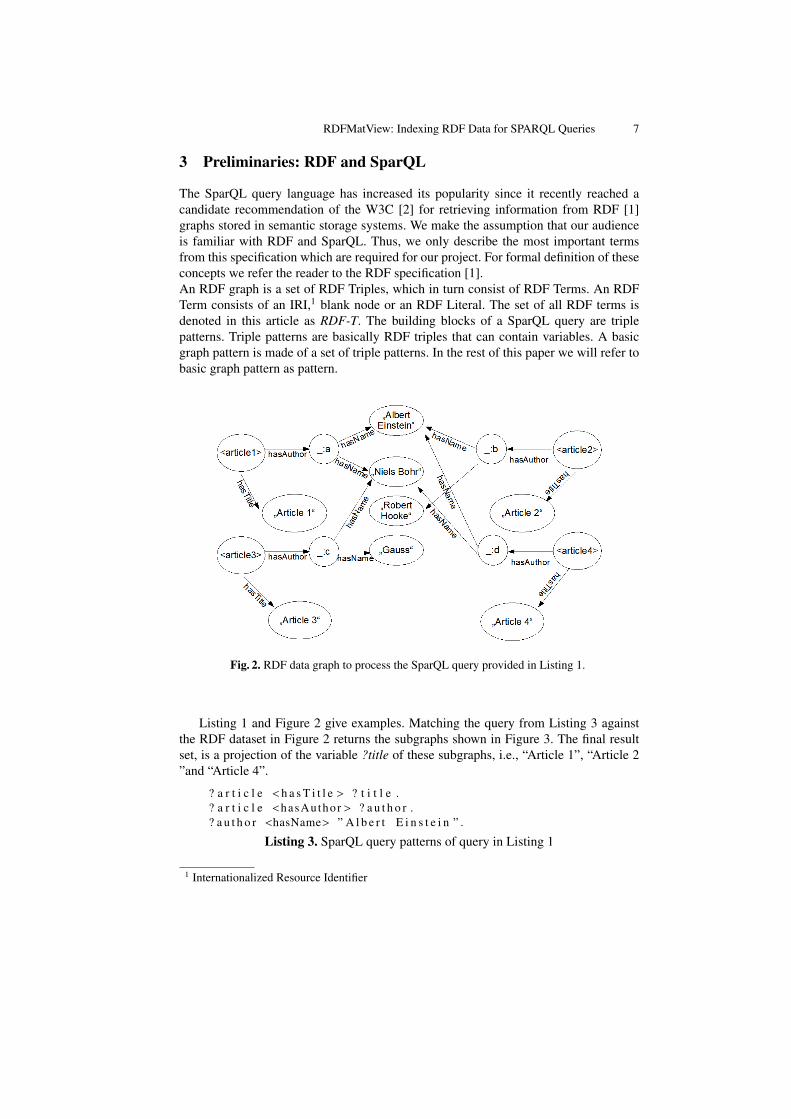
Listing 1 and Figure 2 give examples. Matching the query from Listing 3 againstthe RDF dataset in Figure 2 returns the subgraphs shown in Figure 3. The final resultset, is a projection of the variable ?title of these subgraphs, i.e., “Article 1”, “Article 2”and “Article 4”.
? a r t i c l e <h a s T i t l e > ? t i t l e .? a r t i c l e <hasAuthor > ? a u t h o r .? a u t h o r <hasName> ” A l b e r t E i n s t e i n ” .
Listing 3. SparQL query patterns of query in Listing 1
1 Internationalized Resource Identifier
8 Roger Castillo, Christian Rothe, and Ulf Leser
Fig. 3. Matching subgraphs of query patterns in Listing 3 over data graph in Figure 2.
RDFMatView: Indexing RDF Data for SPARQL Queries 9
4 The RDFMatView Approach
We propose the evaluation of SPARQL queries using other queries that were materi-alized offline. We call those queries materialized queries. In this chapter, we formallyintroduce all necessary concepts for this idea. Section 4.1 defines materialized queriesas indexes and shows how one can decide which of the existing indexes is suitable for agiven query. Those indexes are called eligible, and a set of eligible indexes can be com-bined to cover a query completely or partly. Section 4.2 describes the algorithm whichproduces all possible covers for a query given a set of indexes. An extensive exampleto better explain our ideas is presented in Section 4.3.
4.1 Patterns, Mappings, Occurrences, Indices and Covers
Before we can define an index over RDF graphs we need to explain the concepts ofquery pattern, mapping and occurrence of a pattern. Definitions 1, 2 and 3 introducethese concepts respectively.
Definition 1 (Query Pattern). Let Q be a simple SPARQL query. Then, P(Q) denotesits query pattern, which is the set of triple patterns in the body of Q.
Definition 2 (Mapping, total Mapping). Let P be a query pattern and VP the set ofvariables in P. A mapping is a function defined as follows:
S : VP → RDF-T ∪ V
If S (v) < V for all v ∈ VP, then S is a total mapping.
Our notions of mappings and total mappings is based on the SPARQL-Standard [2]and its definition of pattern solutions. However, while in the SPARQL standard suchsolutions are only searched in the data graph, we also need to permit that variablesare mapped to other variables. This generalization allows us to search occurrences ofpatterns in other patterns, in particular, occurrences of indexes in a query.
Definition 3 (Occurrences of a pattern). Let P1 and P2 be two query patterns. P1 oc-curs in P2, denoted by P1 v P2, iff there is a mapping S such that S (P1) ⊆ P2. Such Sare called embeddings of P1 in P2.
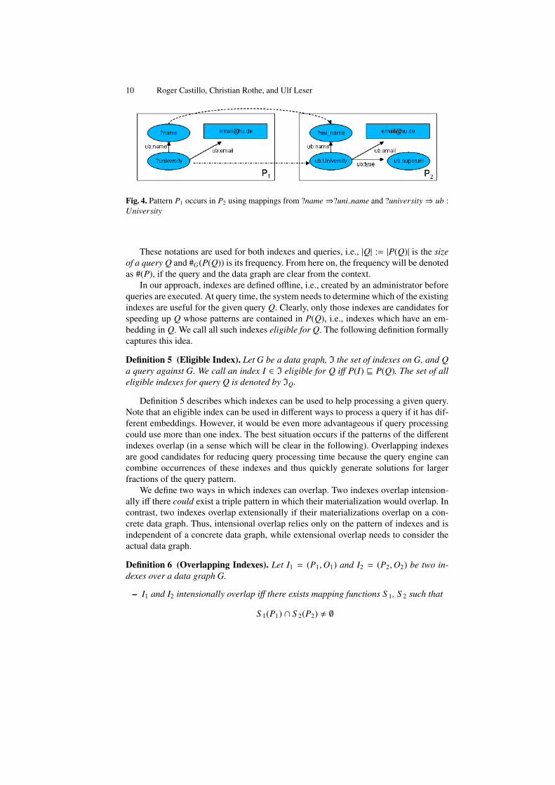
When we speak about a concrete occurrence of an index pattern in a query pattern,we will refer it to as an embedding (to contrast from the term occurrences, which wefrom now on only use for matches of a pattern in the data graph). Figure 4 illustrates anembedding of a pattern P1 in a pattern P2.
Using the previously introduced concepts, we can now define an index over an RDFdata graph.
Definition 4 (Indexes). An index I over a RDF data graph G is a pair I = (P,O),where P represents a query pattern and O represents the set of all occurrences of P inG. P is called the index pattern of I. For an index I = (P,O), the size of I, written as|P|, is the number of triple patterns in P. The frequency of I in G, written as #G(P), isthe number of occurrences of P in G.
10 Roger Castillo, Christian Rothe, and Ulf Leser
Fig. 4. Pattern P1 occurs in P2 using mappings from ?name⇒?uni name and ?university⇒ ub :University
These notations are used for both indexes and queries, i.e., |Q| := |P(Q)| is the sizeof a query Q and #G(P(Q)) is its frequency. From here on, the frequency will be denotedas #(P), if the query and the data graph are clear from the context.
In our approach, indexes are defined offline, i.e., created by an administrator beforequeries are executed. At query time, the system needs to determine which of the existingindexes are useful for the given query Q. Clearly, only those indexes are candidates forspeeding up Q whose patterns are contained in P(Q), i.e., indexes which have an em-bedding in Q. We call all such indexes eligible for Q. The following definition formallycaptures this idea.
Definition 5 (Eligible Index). Let G be a data graph, I the set of indexes on G, and Qa query against G. We call an index I ∈ I eligible for Q iff P(I) v P(Q). The set of alleligible indexes for query Q is denoted by IQ.
Definition 5 describes which indexes can be used to help processing a given query.Note that an eligible index can be used in different ways to process a query if it has dif-ferent embeddings. However, it would be even more advantageous if query processingcould use more than one index. The best situation occurs if the patterns of the differentindexes overlap (in a sense which will be clear in the following). Overlapping indexesare good candidates for reducing query processing time because the query engine cancombine occurrences of these indexes and thus quickly generate solutions for largerfractions of the query pattern.
We define two ways in which indexes can overlap. Two indexes overlap intension-ally iff there could exist a triple pattern in which their materialization would overlap. Incontrast, two indexes overlap extensionally if their materializations overlap on a con-crete data graph. Thus, intensional overlap relies only on the pattern of indexes and isindependent of a concrete data graph, while extensional overlap needs to consider theactual data graph.
Definition 6 (Overlapping Indexes). Let I1 = (P1,O1) and I2 = (P2,O2) be two in-dexes over a data graph G.
– I1 and I2 intensionally overlap iff there exists mapping functions S 1, S 2 such that
S 1(P1) ∩ S 2(P2) , ∅
RDFMatView: Indexing RDF Data for SPARQL Queries 11
– I1 and I2 extensionally overlap in G iff
∃o1 ∈ O1, o2 ∈ O2 : o1 = o2
However, when we want to use overlapping indexes for processing of a query Q,we need to refine our definitions as the query strongly restricts the mappings we needto consider.
Definition 7 (Overlapping Embeddings). Let I1 = (P1,O1) and I2 = (P2,O2) be twoindexes over a data graph G. Let Q be a query over G with P1 ⊆ Q and P2 ⊆ Q, andlet m1 be an embedding of P1 in Q and m2 an embedding of P2 in Q.
– m1 and m2 intentionally overlap in Q iff
m1(P1) ∩ m2(P2) , ∅
– m1 and m2 extensionally overlap in Q and G iff
m1(O1) ∩ m2(O2) , ∅
2
Computing intensional overlaps can be implemented efficiently as this property isindependent from the actual data graph (and updates to it). In contrast, computing ex-tensional overlaps is costly as it requires execution of index queries and comparison oftheir results on a given data graph. On the other hand, at query execution time informa-tion about extensional overlaps would be more important than those about intensionaloverlaps, as the latter is only a necessary yet not sufficient condition for the existence ofa concrete overlap given the query. Actually, if two embeddings intensionally overlapin the query but do not extensionally overlap in the data graph, one can immediatelyconclude that the query has no answer. However, for the rest of this work we onlyconsider intensional overlaps to avoid the costly pre-computation and maintenance ofextensional overlaps.
Using the notion of overlaps, we can finally define the cover of a query.
Definition 8 (Cover). Let Q be a query and EQ the set of all embeddings of eligibleindexes for Q in Q. Let C ⊆ EQ. Build a graph GC for C as follows: Each embeddingin C is represented as a node. Whenever two embeddings from C intensionally overlapin Q, we add an edge to GC between the nodes representing the embeddings. Any C forwhich GC has only one connected component is called a cover for Q.
We focus on covers with overlapping embeddings since they allow better estima-tions of the cost savings that can be achieved with them (see next Section). Furthermore,we are only interested in maximal covers, i.e., those covers which cannot be extendedfurther by adding new embeddings.
2 With slight abuse of notation. By m1(O1) we mean the projection of all occurrences in O1 usingm1.
12 Roger Castillo, Christian Rothe, and Ulf Leser
Definition 9 (Maximal Covers). Let Q be a query and C1 , C2 be two covers for Q.C1 is subsumed by C2 if C1 ⊆ C2. Any cover which is not subsumed by another cover iscalled maximal.
In the following, we only consider maximal covers. We classify those into two dif-ferent groups:
– A cover is complete if it covers all patterns of a query.– A cover is partial if it is not complete.
Usually it is not possible to find a complete cover of a query. According to this, werefer in the rest of this article to a partial cover as a cover.
4.2 Finding covers
Definition 8 is purely conceptual. We now show how we actually compute the set ofindexes and how we combine their embeddings to find all covers.
The first task is performed by a adaption of the classical algorithms for query con-tainment of relational queries [17]. Essentially, we find all mappings between any indexpattern and the query pattern by enumerating all possible cases. If an mapping existsthen we can conclude that an index is eligible for that query and we store mapping asan embedding. Note that, for a given index, there are potentially many different waysto be eligible, i.e., different mappings between index and query patterns and therefore,multiple embeddings. Algorithm 1 illustrates this process.
Algorithm 1 Pseudo code for SPARQL query containment. The algorithm computesall embeddings of indexes in a given query.Given: Query Q, set of indexes IReturns: Set EQ of all embeddings1: P(I), P(Q) {index and query patterns}2: O := ∅ {Set of embeddings of P(I) in P(Q)}3: EQ := ∅ {Set of all embeddings}4: for all Index I in I do5: O := S |S (P(I)) = P(Q)6: if O <> ∅ then7: EQ = EQ ∪O8: end if9: end for
The core of algorithm 1 is line 5 which computes all embeddings of an index inthe query pattern. The implementation of this step is shown in in Algorithm 2 whichtraverses a tree representing the search space of all possible mappings from the indexinto the query. Each level in the tree contains all mappings for a specific triple pattern.All mappings of a level in the tree are children of each mapping of the previous level.In Line 12 we generate this tree and traverse it using backtracking in Line 13. Duringthe traversal, the mappings for the different triples are combined (if compatible) to
RDFMatView: Indexing RDF Data for SPARQL Queries 13
increasingly larger mappings. Whenever all triples of the index have been mapped tothe query pattern by one mapping, this mapping is added to the set of embeddings.
Algorithm 2 Pseudo code for searching all embeddings of an index in a query patterns.It maps variables from the index to the queryGiven: Query pattern P(Q), index pattern P(I)Returns: O, set of embeddings of P(I) in P(Q)1: Lt := ∅ {Temporal list of occurrences of each index triple pattern in P(Q)}2: L := ∅ {Total list of ti occurrences in P(Q)}3: for all Triple Pattern ti in P(I) do4: for all Triple Pattern tq in P(Q) do5: if ti occurs in tq with mapping S then6: Lt := Lt ∪ S7: end if8: end for9: L := L ∪ Lt
10: Lt := ∅11: end for12: occTree := createTree(L)13: return O := traverseTree(occTree)
Once we have all embeddings, we proceed to generate covers. To this end, we firstcompute all mutual intensional overlaps between indexes and store them in a matrix. Wethen incrementally build maximal covers by finding all maximal connected componentsin this matrix.
4.3 Example
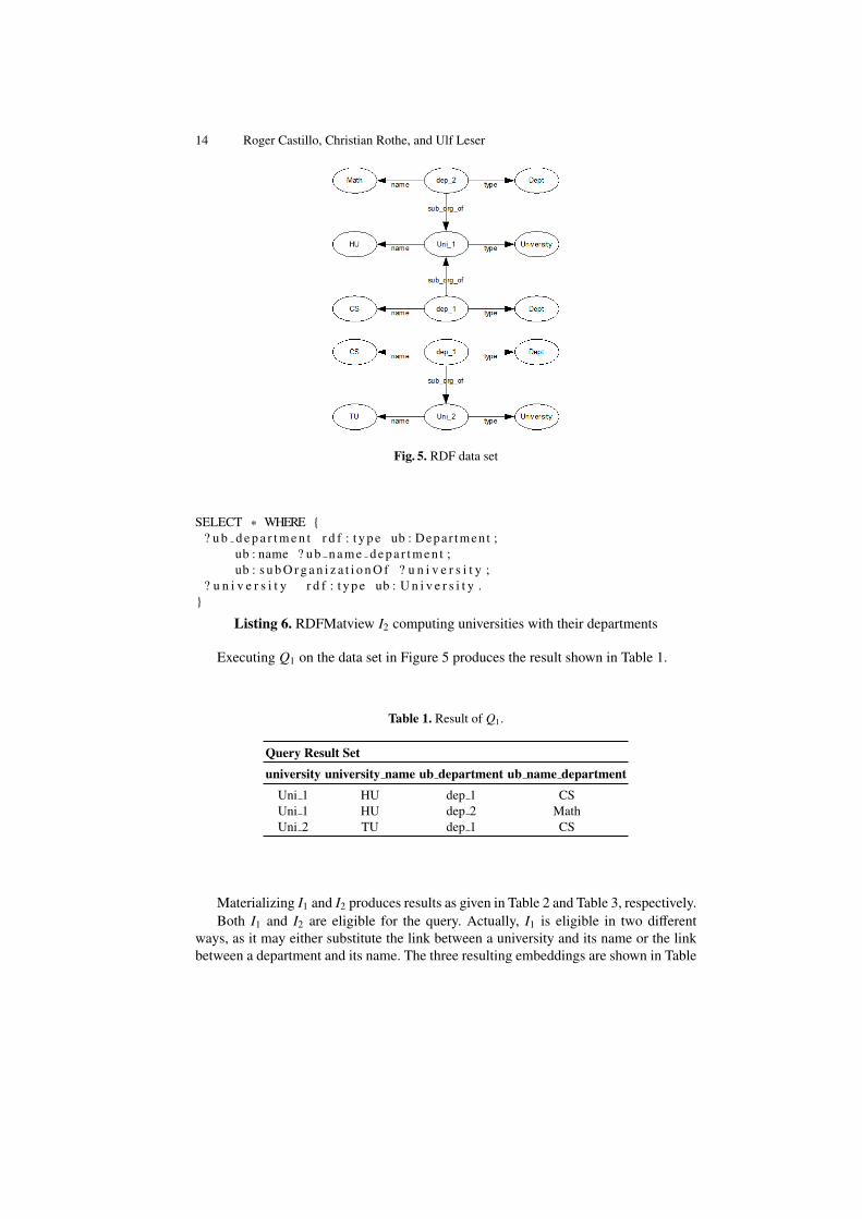
We illustrate all previously introduced concepts using a comprehensive example. Con-sider the RDF data listed in Figure 5, the SPARQL query Q1 shown in Listing 4, andthe two RDFMatView indexes I1, I2 from Listing 5 and 6, respectively.
SELECT ∗ WHERE {? u n i v e r s i t y r d f : t y p e ub : U n i v e r s i t y ;
ub : name ? u n i v e r s i t y n a m e .? u b d e p a r t m e n t r d f : t y p e ub : Depar tment ;
ub : name ? u b n a m e d e p a r t m e n t ;ub : s u b O r g a n i z a t i o n O f ? u n i v e r s i t y .
}
Listing 4. SPARQL query Q1 computing universities and their departments
SELECT ∗ WHERE {? p l a c e r d f : t y p e ? p l a c e t y p e ;
ub : name ? p lace name .}
Listing 5. RDFMatview I1 computing places and their names
14 Roger Castillo, Christian Rothe, and Ulf Leser
Fig. 5. RDF data set
SELECT ∗ WHERE {? u b d e p a r t m e n t r d f : t y p e ub : Depar tment ;
ub : name ? u b n a m e d e p a r t m e n t ;ub : s u b O r g a n i z a t i o n O f ? u n i v e r s i t y ;
? u n i v e r s i t y r d f : t y p e ub : U n i v e r s i t y .}
Listing 6. RDFMatview I2 computing universities with their departments
Executing Q1 on the data set in Figure 5 produces the result shown in Table 1.
Table 1. Result of Q1.
Query Result Setuniversity university name ub department ub name department
Uni 1 HU dep 1 CSUni 1 HU dep 2 MathUni 2 TU dep 1 CS
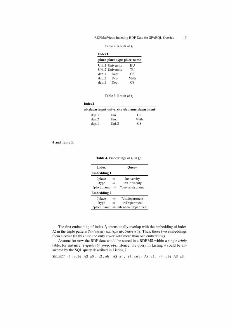
Materializing I1 and I2 produces results as given in Table 2 and Table 3, respectively.Both I1 and I2 are eligible for the query. Actually, I1 is eligible in two different
ways, as it may either substitute the link between a university and its name or the linkbetween a department and its name. The three resulting embeddings are shown in Table
RDFMatView: Indexing RDF Data for SPARQL Queries 15
Table 2. Result of I1.
Index1place place type place nameUni 1 University HUUni 2 University TUdep 1 Dept CSdep 2 Dept Mathdep 1 Dept CS
Table 3. Result of I2.
Index2ub department university ub name department
dep 1 Uni 1 CSdep 2 Uni 1 Mathdep 1 Uni 2 CS
4 and Table 5.
Table 4. Embeddings of I1 in Q1.
Index QueryEmbedding 1
?place ⇒ ?university?type ⇒ ub:University
?place name ⇒ ?university name
Embedding 2?place ⇒ ?ub department?type ⇒ ub:Department
?place name ⇒ ?ub name department
The first embedding of index I1 intensionally overlap with the embedding of indexI2 in the triple pattern ?university rdf:type ub:University. Thus, these two embeddingsform a cover (in this case the only cover with more than one embedding).
Assume for now the RDF data would be stored in a RDBMS within a single tripletable, for instance, Triple(subj, prop, obj). Hence, the query in Listing 4 could be an-swered by the SQL query described in Listing 7.
SELECT t 1 . s u b j AS a0 , t 2 . o b j AS a1 , t 3 . s u b j AS a2 , t 4 . o b j AS a3
16 Roger Castillo, Christian Rothe, and Ulf Leser
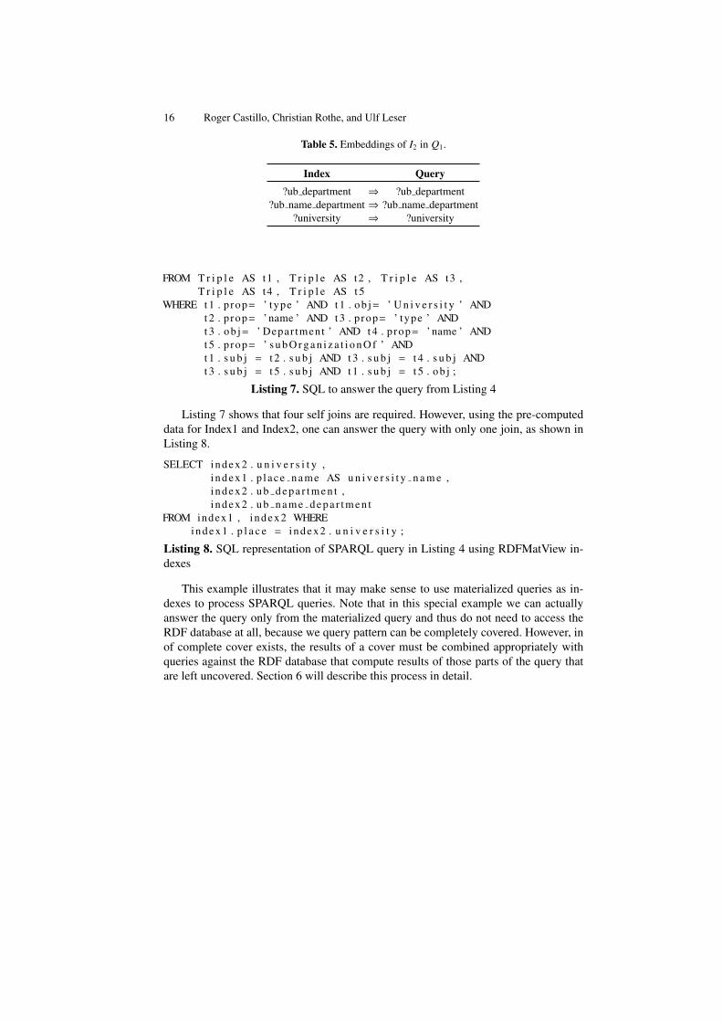
Table 5. Embeddings of I2 in Q1.
Index Query?ub department ⇒ ?ub department
?ub name department ⇒ ?ub name department?university ⇒ ?university
FROM T r i p l e AS t1 , T r i p l e AS t2 , T r i p l e AS t3 ,T r i p l e AS t4 , T r i p l e AS t 5
WHERE t 1 . prop= ’ type ’ AND t 1 . o b j= ’ U n i v e r s i t y ’ ANDt 2 . prop= ’ name ’ AND t 3 . prop= ’ type ’ ANDt 3 . o b j= ’ Depar tment ’ AND t 4 . prop= ’ name ’ ANDt 5 . prop= ’ s u b O r g a n i z a t i o n O f ’ ANDt 1 . s u b j = t 2 . s u b j AND t 3 . s u b j = t 4 . s u b j ANDt 3 . s u b j = t 5 . s u b j AND t 1 . s u b j = t 5 . o b j ;
Listing 7. SQL to answer the query from Listing 4
Listing 7 shows that four self joins are required. However, using the pre-computeddata for Index1 and Index2, one can answer the query with only one join, as shown inListing 8.
SELECT in de x2 . u n i v e r s i t y ,i n de x1 . p l ace name AS u n i v e r s i t y n a m e ,in de x2 . u b d e p a r t m e n t ,i n de x2 . u b n a m e d e p a r t m e n t
FROM index1 , i nd ex 2 WHEREin de x1 . p l a c e = i n de x2 . u n i v e r s i t y ;
Listing 8. SQL representation of SPARQL query in Listing 4 using RDFMatView in-dexes
This example illustrates that it may make sense to use materialized queries as in-dexes to process SPARQL queries. Note that in this special example we can actuallyanswer the query only from the materialized query and thus do not need to access theRDF database at all, because we query pattern can be completely covered. However, inof complete cover exists, the results of a cover must be combined appropriately withqueries against the RDF database that compute results of those parts of the query thatare left uncovered. Section 6 will describe this process in detail.
RDFMatView: Indexing RDF Data for SPARQL Queries 17
5 Cost Model
In the previous sections we defined which indexes and which sets of indexes, i.e., cov-ers, are eligible for a given query. At run time, the optimizer must choose between thesedifferent options, or decide to execute the query without using indexes. This decisionshould be taken based on the expected savings in time that the usage of one or moreindexes brings to query execution. In the following, we define a simple model for es-timating these savings. This model implicitly makes a number of assumptions on thedata graph. For instance, we treat all triples of a pattern equally with respect to their ex-pected numbers of matches, independent of whether or not the triple contains variables,and independent of the real frequency of constants. These assumptions make the modelvery simple and also allow us to estimate query costs without any detailed knowledgeof the underlying database. Clearly, finding more detailed cost models is an importantfuture work.
Our model estimates the cost of executing a query with zero, one, or more indexes.Note that it is not the purpose of the model to directly estimate the necessary executiontime, as it depends on a multitude of factors which are extremely difficult to model (suchas processing strategy, size of data sets, hardware etc.). In contrast, our model onlyaims at discerning good plans from bad plans; to this end, the estimated cost only mustcorrelate with the real time. We shall evaluate the quality of our cost model empiricallyin Section 7.
Our model is based on the following fundamental observations. For each index Ithat occurs in the query pattern, each occurrence of the query pattern in the data graphmust contain an occurrence of I. This leads to following facts:
1. It makes sense to prefer those indexes which have few occurrences because everyoccurrence of an index must be validated to verify the possibility to extend it to anoccurrence of the query.
2. It is reasonable to cover as much as possible from the query patterns. This processreduces the number of query patterns that need to be evaluated against the datagraph. According to this, large index patterns are specially interesting.
We formally capture these observations in the definition of the selectivity of anindex. It defines the relation of the number of occurrences of an index in a given graphto the possible total number of index occurrences in the graph. To calculate selectivity,we need the size and the frequency of the index pattern as well as the size of the datagraph.
Definition 10 (Selectivity of an index). Let I be an index over a data graph G. Theselectivity s(I) of I is defined as:
s(I) =#(I)
|G||I|.
We derive our formula for estimating the selectivity of a set I of indexes from theprevious definition. To this end, we view I as the union of the patterns of the indexesin I (similar to the union of RDF graphs, see [18]). Without further knowledge, the
18 Roger Castillo, Christian Rothe, and Ulf Leser
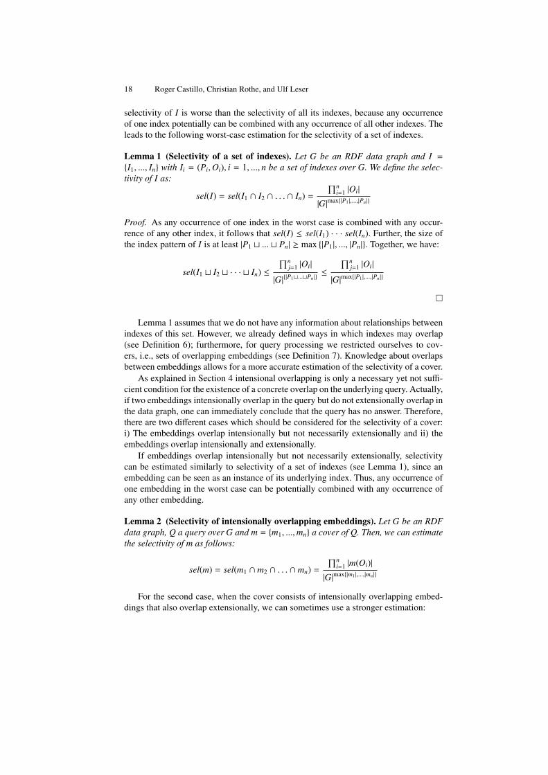
selectivity of I is worse than the selectivity of all its indexes, because any occurrenceof one index potentially can be combined with any occurrence of all other indexes. Theleads to the following worst-case estimation for the selectivity of a set of indexes.
Lemma 1 (Selectivity of a set of indexes). Let G be an RDF data graph and I =
{I1, ..., In} with Ii = (Pi,Oi), i = 1, ..., n be a set of indexes over G. We define the selec-tivity of I as:
sel(I) = sel(I1 ∩ I2 ∩ . . . ∩ In) =
∏ni=1 |Oi|
|G|max{|P1 |,...,|Pn |}
Proof. As any occurrence of one index in the worst case is combined with any occur-rence of any other index, it follows that sel(I) ≤ sel(I1) · · · sel(In). Further, the size ofthe index pattern of I is at least |P1 t ... t Pn| ≥ max {|P1|, ..., |Pn|}. Together, we have:
sel(I1 t I2 t · · · t In) ≤
∏nj=1 |Oi|
|G|{|P1t...tPn |}≤
∏nj=1 |Oi|
|G|max{|P1 |,...,|Pn |}
�
Lemma 1 assumes that we do not have any information about relationships betweenindexes of this set. However, we already defined ways in which indexes may overlap(see Definition 6); furthermore, for query processing we restricted ourselves to cov-ers, i.e., sets of overlapping embeddings (see Definition 7). Knowledge about overlapsbetween embeddings allows for a more accurate estimation of the selectivity of a cover.
As explained in Section 4 intensional overlapping is only a necessary yet not suffi-cient condition for the existence of a concrete overlap on the underlying query. Actually,if two embeddings intensionally overlap in the query but do not extensionally overlap inthe data graph, one can immediately conclude that the query has no answer. Therefore,there are two different cases which should be considered for the selectivity of a cover:i) The embeddings overlap intensionally but not necessarily extensionally and ii) theembeddings overlap intensionally and extensionally.
If embeddings overlap intensionally but not necessarily extensionally, selectivitycan be estimated similarly to selectivity of a set of indexes (see Lemma 1), since anembedding can be seen as an instance of its underlying index. Thus, any occurrence ofone embedding in the worst case can be potentially combined with any occurrence ofany other embedding.
Lemma 2 (Selectivity of intensionally overlapping embeddings). Let G be an RDFdata graph, Q a query over G and m = {m1, ...,mn} a cover of Q. Then, we can estimatethe selectivity of m as follows:
sel(m) = sel(m1 ∩ m2 ∩ . . . ∩ mn) =
∏ni=1 |m(Oi)|
|G|max{|m1 |,...,|mn |}
For the second case, when the cover consists of intensionally overlapping embed-dings that also overlap extensionally, we can sometimes use a stronger estimation:
RDFMatView: Indexing RDF Data for SPARQL Queries 19
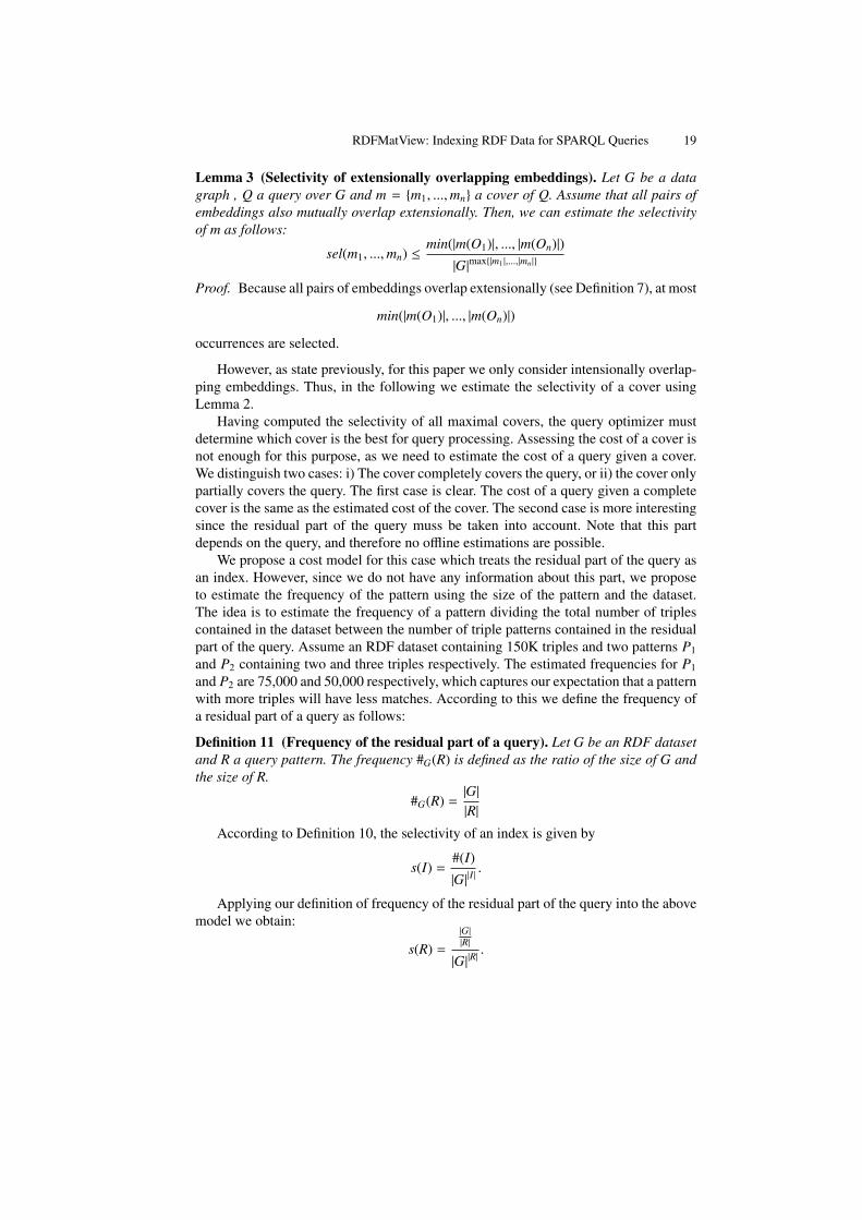
Lemma 3 (Selectivity of extensionally overlapping embeddings). Let G be a datagraph , Q a query over G and m = {m1, ...,mn} a cover of Q. Assume that all pairs ofembeddings also mutually overlap extensionally. Then, we can estimate the selectivityof m as follows:
sel(m1, ...,mn) ≤min(|m(O1)|, ..., |m(On)|)
|G|max{|m1 |,...,|mn |}
Proof. Because all pairs of embeddings overlap extensionally (see Definition 7), at most
min(|m(O1)|, ..., |m(On)|)
occurrences are selected.
However, as state previously, for this paper we only consider intensionally overlap-ping embeddings. Thus, in the following we estimate the selectivity of a cover usingLemma 2.
Having computed the selectivity of all maximal covers, the query optimizer mustdetermine which cover is the best for query processing. Assessing the cost of a cover isnot enough for this purpose, as we need to estimate the cost of a query given a cover.We distinguish two cases: i) The cover completely covers the query, or ii) the cover onlypartially covers the query. The first case is clear. The cost of a query given a completecover is the same as the estimated cost of the cover. The second case is more interestingsince the residual part of the query muss be taken into account. Note that this partdepends on the query, and therefore no offline estimations are possible.
We propose a cost model for this case which treats the residual part of the query asan index. However, since we do not have any information about this part, we proposeto estimate the frequency of the pattern using the size of the pattern and the dataset.The idea is to estimate the frequency of a pattern dividing the total number of triplescontained in the dataset between the number of triple patterns contained in the residualpart of the query. Assume an RDF dataset containing 150K triples and two patterns P1and P2 containing two and three triples respectively. The estimated frequencies for P1and P2 are 75,000 and 50,000 respectively, which captures our expectation that a patternwith more triples will have less matches. According to this we define the frequency ofa residual part of a query as follows:
Definition 11 (Frequency of the residual part of a query). Let G be an RDF datasetand R a query pattern. The frequency #G(R) is defined as the ratio of the size of G andthe size of R.
#G(R) =|G||R|
According to Definition 10, the selectivity of an index is given by
s(I) =#(I)
|G||I|.
Applying our definition of frequency of the residual part of the query into the abovemodel we obtain:
s(R) =
|G||R|
|G||R|.

20 Roger Castillo, Christian Rothe, and Ulf Leser
simplifying the equation, results in the following model:
Definition 12 (Selectivity of the residual part of a query). Let G be an RDF datasetand R a query pattern. The selectivity of R is defined as:
s(R) =1
|R| · |G||R−1| .
Finally, based on Lemma 2 and Definition 12 we define the estimated cost for aSPARQL query given a cover as follows.
Definition 13 (Estimated cost for a query given a cover). Let Q be a SPARQL query,C a cover of Q and R the residual patterns of Q, i.e., the triples from P(Q) not coveredby C. Then, we estimate the cost of execution Q using C as
c(Q,C) = sel(C) · sel(R)
RDFMatView: Indexing RDF Data for SPARQL Queries 21
6 Implementation
In this section, we describe how our approach can be integrated into an existing SPARQLquery processor. Such an integration touches upon several components of a system:First, we need to be able to execute index queries and to store their results (plus somemetadata) persistently. To use indexes in query processing, we need to intercept thequery processor to, at the right point in time, search for an optimal cover. Finally, wemust change the way how queries are executed, as we need to divide the query patterninto that part that is covered by the chosen cover - which is answered by retrieval of thematerialized information - and the rest of the query pattern. We present solutions to allthese steps for the ARQ system [19]. However, we want to stress that general processwould be the same for any other SPARQL query processors.
In this chapter, we first give some details on ARQ and Jena, its storage model. Wethen provide a high level description of our approach. Next, we show how an indexis made persistent using a data dictionary for saving space. Finally, we describe threeways in which query processing in ARQ can integrate materialized queries as indexes.Those will be evaluated separately in the next chapter.
6.1 ARQ and the Jena Persistent Storage Schema
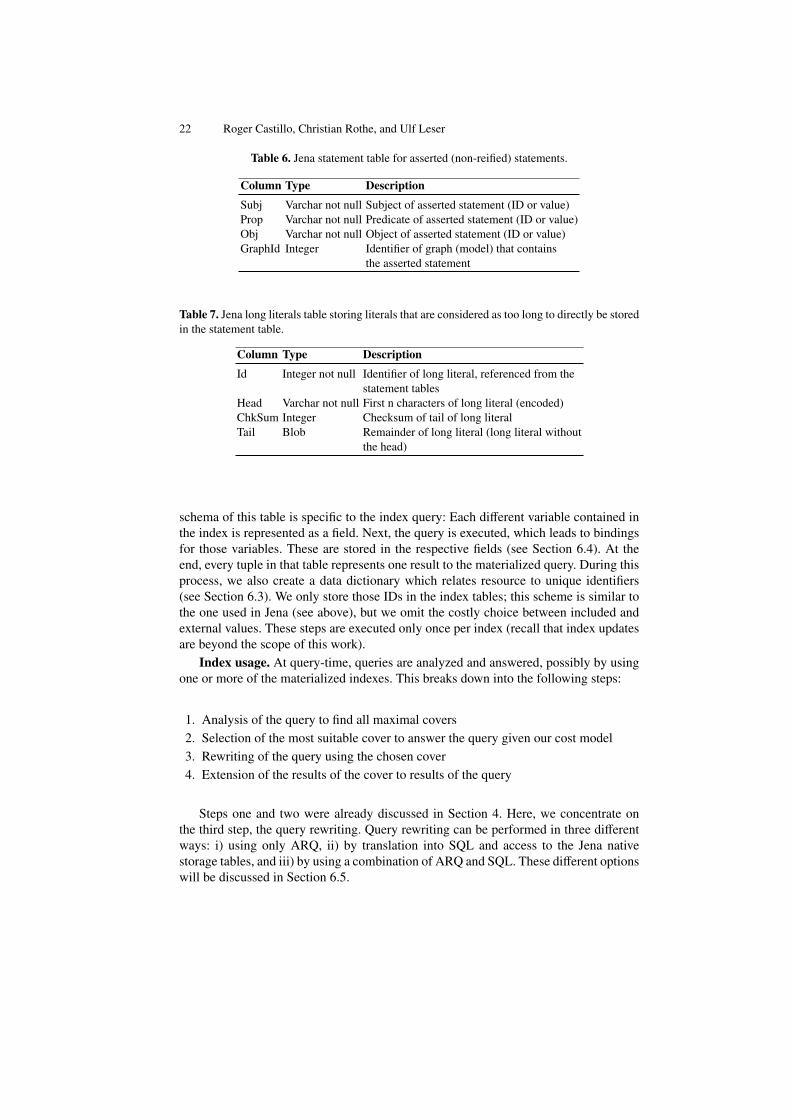
For our integration with ARQ we use the Jena persistence subsystem. This subsystemimplements the Jena Model interface using a back-end relational database engine. Thedefault Jena database layout uses a denormalized schema centered around a statementtable which essentially stores every RDF tripel as tuple. However, the values in the triplecan either be included as value, or they are stored in other tables. Specifically, shortliterals are stored directly in the statement table, while long literals are stored in a literaltable. Similarly, short URIs are stored in the statement table and long URIs are storedin a resources table. Table 6 and Table 7 describe the layout for those tables. Thoughthis scheme helps to reduce space requirements especially in the presence of long andfrequently used URIs or labels, it makes query processing more complicated as, for eachrow in the statement table, one must decide at runtime whether the respective value canbe obtained directly or if a a join to another table is necessary. that it stores reifiedstatements in an optimized form. Recall that a reified statement is expressed in RDF asfour individual RDF statements. Storing this would require four rows in the standardrepresentation, while the reified statement table stores each statement in a single row.For applications that use a large number of reified statements, the space savings canbe substantial. Additionally, Jena defines system tables to store meta data. For furtherinformation we refer the reader to [3].
6.2 Implementation overview
We differentiate two phases. At offline-time, indexes are created, analyzed, and theirresults are materialized. At query-time, queries are answered with the help of indexes.We divide our description of our implementation according to these phases.
Index creation. Indexes are created offline. Upon creation of an index, the followingthings happen. First, a new table is created which will store the materialized query. The
22 Roger Castillo, Christian Rothe, and Ulf Leser
Table 6. Jena statement table for asserted (non-reified) statements.
Column Type DescriptionSubj Varchar not null Subject of asserted statement (ID or value)Prop Varchar not null Predicate of asserted statement (ID or value)Obj Varchar not null Object of asserted statement (ID or value)GraphId Integer Identifier of graph (model) that contains
the asserted statement
Table 7. Jena long literals table storing literals that are considered as too long to directly be storedin the statement table.
Column Type DescriptionId Integer not null Identifier of long literal, referenced from the
statement tablesHead Varchar not null First n characters of long literal (encoded)ChkSum Integer Checksum of tail of long literalTail Blob Remainder of long literal (long literal without
the head)
schema of this table is specific to the index query: Each different variable contained inthe index is represented as a field. Next, the query is executed, which leads to bindingsfor those variables. These are stored in the respective fields (see Section 6.4). At theend, every tuple in that table represents one result to the materialized query. During thisprocess, we also create a data dictionary which relates resource to unique identifiers(see Section 6.3). We only store those IDs in the index tables; this scheme is similar tothe one used in Jena (see above), but we omit the costly choice between included andexternal values. These steps are executed only once per index (recall that index updatesare beyond the scope of this work).
Index usage. At query-time, queries are analyzed and answered, possibly by usingone or more of the materialized indexes. This breaks down into the following steps:
1. Analysis of the query to find all maximal covers2. Selection of the most suitable cover to answer the query given our cost model3. Rewriting of the query using the chosen cover4. Extension of the results of the cover to results of the query
Steps one and two were already discussed in Section 4. Here, we concentrate onthe third step, the query rewriting. Query rewriting can be performed in three differentways: i) using only ARQ, ii) by translation into SQL and access to the Jena nativestorage tables, and iii) by using a combination of ARQ and SQL. These different optionswill be discussed in Section 6.5.
RDFMatView: Indexing RDF Data for SPARQL Queries 23
6.3 RDF Data Dictionary
As triples may contain long string literals, we generate a data dictionary that maps alldifferent RDF terms to a unique ID. This has two main benefits: 1) It decreases thespace requirements of indexes, and 2) it is a simplification for the query processor sinceit will have to deal only with numerical values instead of string values. This makes adifference as, depending upon the specific strategy for query processing chosen, valuesmight have to go back-and-forth between the database and the query processor. Thecost for this gains is that at the end of query evaluation, all IDs need to be translatedinto the original values.
Listing 8 illustrates the schema of our RDF data dictionary.
Table 8. RDF Data Dictionary
Column Type DescriptionIDResource bigint not null Resource identifier (encoded)Resource Varchar not null Original resource value
6.4 RDFMatView Index processing
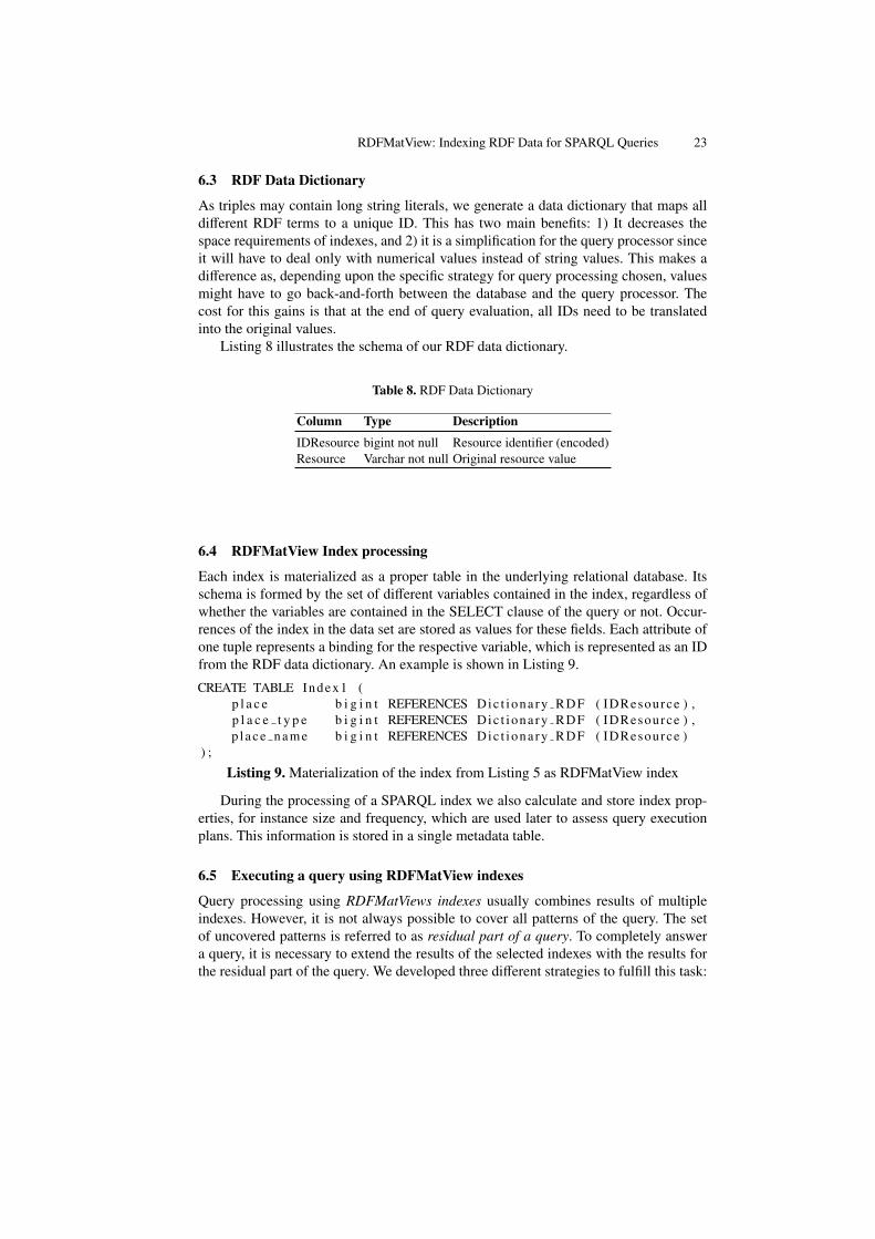
Each index is materialized as a proper table in the underlying relational database. Itsschema is formed by the set of different variables contained in the index, regardless ofwhether the variables are contained in the SELECT clause of the query or not. Occur-rences of the index in the data set are stored as values for these fields. Each attribute ofone tuple represents a binding for the respective variable, which is represented as an IDfrom the RDF data dictionary. An example is shown in Listing 9.
CREATE TABLE Index1 (p l a c e b i g i n t REFERENCES Dic t iona ry RDF ( IDResource ) ,p l a c e t y p e b i g i n t REFERENCES Dic t iona ry RDF ( IDResource ) ,p l ace name b i g i n t REFERENCES Dic t iona ry RDF ( IDResource )
) ;
Listing 9. Materialization of the index from Listing 5 as RDFMatView index
During the processing of a SPARQL index we also calculate and store index prop-erties, for instance size and frequency, which are used later to assess query executionplans. This information is stored in a single metadata table.
6.5 Executing a query using RDFMatView indexes
Query processing using RDFMatViews indexes usually combines results of multipleindexes. However, it is not always possible to cover all patterns of the query. The setof uncovered patterns is referred to as residual part of a query. To completely answera query, it is necessary to extend the results of the selected indexes with the results forthe residual part of the query. We developed three different strategies to fulfill this task:
24 Roger Castillo, Christian Rothe, and Ulf Leser
– Our first strategy uses ARQ to process the residual part of the query. RDFMatViewextends the results of the chosen cover by joining the partial solutions with thesolutions of the residual patterns.
– The second strategy is based on a SPARQL-to-SQL algorithm. The idea is to di-rectly access the native Jena storage tables and to combine those results with theindex tables to generate the final result set.
– The last strategy is a combination of the previous two strategies, i.e. ARQ queryengine and database execution engine.
These strategies are explained in detail in the next sections.
Method 1: MatView-and-ARQ Engine
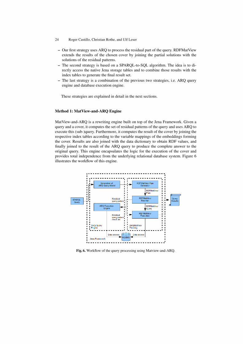
MatView-and-ARQ is a rewriting engine built on top of the Jena Framework. Given aquery and a cover, it computes the set of residual patterns of the query and uses ARQ toexecute this (sub-)query. Furthermore, it computes the result of the cover by joining therespective index tables according to the variable mappings of the embeddings formingthe cover. Results are also joined with the data dictionary to obtain RDF values, andfinally joined to the result of the ARQ query to produce the complete answer to theoriginal query. This engine encapsulates the logic for the execution of the cover andprovides total independence from the underlying relational database system. Figure 6illustrates the workflow of this engine.
Fig. 6. Workflow of the query processing using Matview-and-ARQ.
RDFMatView: Indexing RDF Data for SPARQL Queries 25
Method 2: MatView-to-SQL Engine
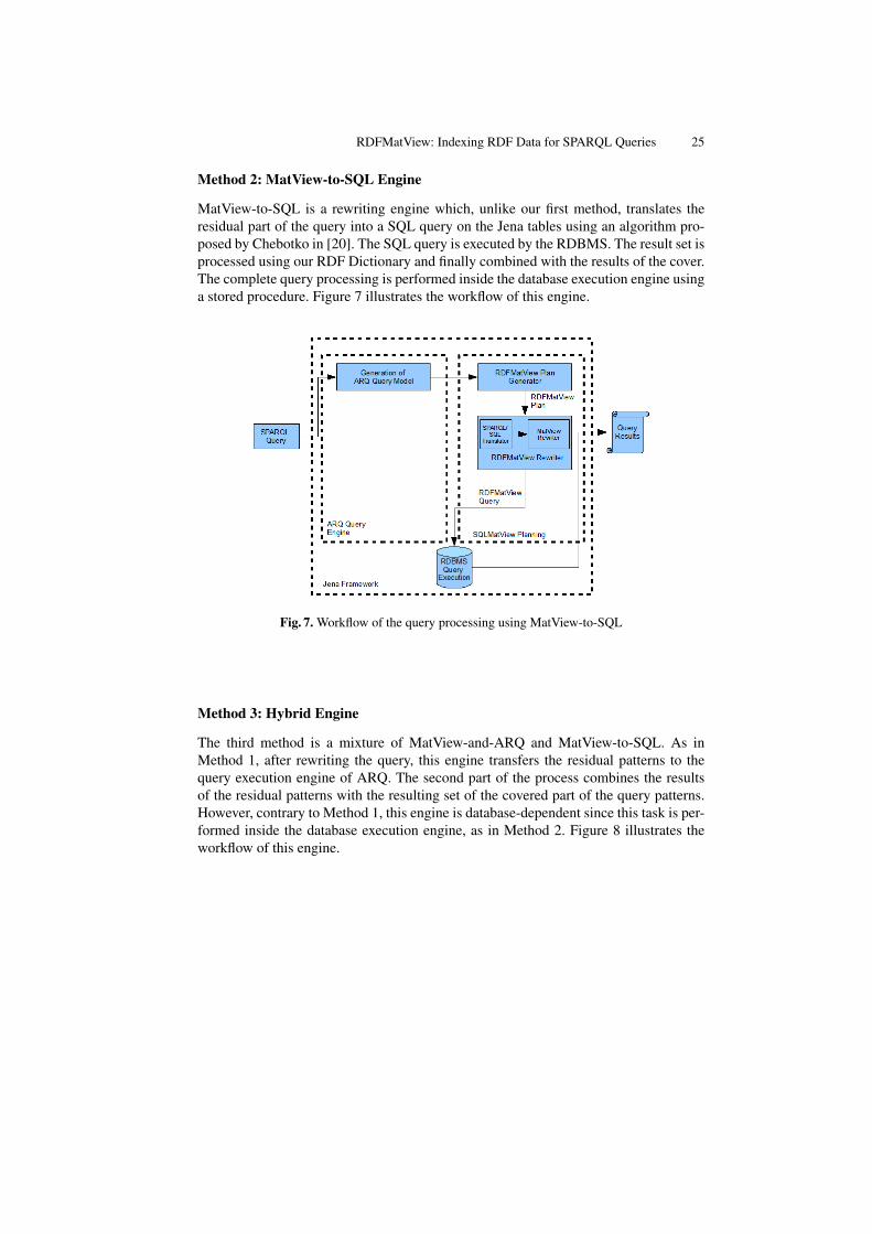
MatView-to-SQL is a rewriting engine which, unlike our first method, translates theresidual part of the query into a SQL query on the Jena tables using an algorithm pro-posed by Chebotko in [20]. The SQL query is executed by the RDBMS. The result set isprocessed using our RDF Dictionary and finally combined with the results of the cover.The complete query processing is performed inside the database execution engine usinga stored procedure. Figure 7 illustrates the workflow of this engine.
Fig. 7. Workflow of the query processing using MatView-to-SQL
Method 3: Hybrid Engine
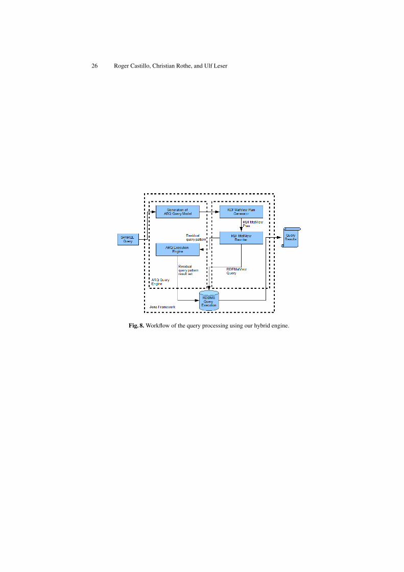
The third method is a mixture of MatView-and-ARQ and MatView-to-SQL. As inMethod 1, after rewriting the query, this engine transfers the residual patterns to thequery execution engine of ARQ. The second part of the process combines the resultsof the residual patterns with the resulting set of the covered part of the query patterns.However, contrary to Method 1, this engine is database-dependent since this task is per-formed inside the database execution engine, as in Method 2. Figure 8 illustrates theworkflow of this engine.
26 Roger Castillo, Christian Rothe, and Ulf Leser
Fig. 8. Workflow of the query processing using our hybrid engine.
RDFMatView: Indexing RDF Data for SPARQL Queries 27
7 Evaluation
In this section, we describe a preliminary evaluation of our approach using the BerlinSPARQL Benchmark. This benchmark allows the creation of data sets with config-urable sizes [21]. We generated five RDF datasets with sizes ranging from 250K to25M triples and tested the respective impact of indexes using three queries from thebenchmark set. For each of these queries, we created a range of different indexes, lead-ing to covers composed of one to three embeddings. Note that it is not our intention tofind the best set of indexes given a workload (which is generally called index selection,see, e.g., [22–24]); instead, we want to study to which degree different indexes usingdifferent processing schemes speed up the execution of queries. As SPARQL processor,we use the ARQ/Jena RDF Storage System (version 2.5.7) on Postgres 8.2.
In the following, we first briefly introduce the Berlin SPARQL Benchmark. We thendescribe the datasets and test queries as well as the indexes we used. Finally, we presentand discuss the results of our evaluation.
7.1 Berlin SPARQL Benchmark
The Berlin SPARQL benchmark is built on an e-commerce use case in which a setof products is offered by different vendors and where consumers have posted reviewsabout products [21]. The main classes of its schema are:
– Product Captures products with different sets of properties and features.– ProductType Classifies products into a hierarchy.– ProductFeature Represents product features for a specific product depending on
the product type. Each product type in the hierarchy has a set of associated productfeatures, which leads to some features being very generic and others being morespecific.
– Producer Represents the producer of products.– Vendor Represents the supplier of products.– Offer Describes an offer to a product.– Person Captures all person-related information.– Review Provides ratings of a product.
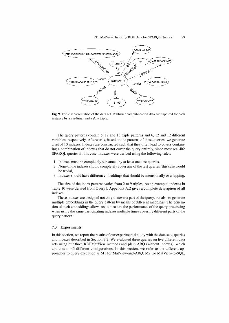
The benchmark provides a data generator which supports the creation of arbitrarilylarge datasets using the number of products as scale factor. Table 9 provides a detaileddescription of the datasets using three different scale factors, and Figure 9 illustrates atriple representation of the generated data.
The benchmark also defines a set of SPARQL queries to simulate a use-case drivenworkload. This set emulates the search and navigation pattern of a consumer lookingfor a product. Basically, the sequence of queries performs the following operations:
1. A consumer searches for products that have a set of general features.2. From the returning set of products, the consumer has a better idea of what he wants
and restricts his search with more specific features.3. The consumer starts to look at specific products and recent reviews for these.
28 Roger Castillo, Christian Rothe, and Ulf Leser
4. To check the trustworthiness of the reviews, the consumer retrieves backgroundinformation about the reviewers.
5. The consumer decides which product to buy and starts to search for the best pricefor this product offered by a vendor that is located in his country and is able todeliver within three days.
6. After choosing a specific offer, the consumer retrieves all information about theoffer and then transforms the information into another schema in order to save itlocally for future reference.
These use cases are reflected by a total of 12 different queries.
Table 9. Berlin SPARQL benchmark. Scaling and dataset population. The number of products isused as scale factor.
Number of Products 666 2,785 70,812Number of RDF Triples 250,000 1,000,000 25,000,000Number of Producers 14 60 1,422Number of Product Features 2,860 4,745 23,833Number of Product Types 55 151 731Number of Vendors 8 34 722Number of Offers 13,320 55,700 1,416,240Number of Reviewers 339 1,432 36,249Number of Reviews 6,660 27,850 708,120Number of Instances 23,922 92,757 2,258,129File size Turtle (unzipped) 22 Mb 86 Mb 2.1 Gb
7.2 Dataset and queries
The performance of our solution is evaluated over five data sets containing 250K, 500K,1M, 10M and 25M triples. As these data sets have identical value distributions butdifferent sizes, evaluation can fully concentrate on the scalability of our methods. Basedon their number of triple patterns, we chose three of the queries from the benchmarks setfor experimentation. We transformed the query patterns into simple graph patterns (theonly form of patterns our current implementation can cope with) and removed bindingsto variables. Bounded variables incur extremely high selectivity resulting in the retrievalof only a handful of triples. Such queries are well supported by existing index structuresin RDBMS and do not require the type of join-optimization that is achieved with ouroptimization technique; therefore, performance gains would be only marginal.
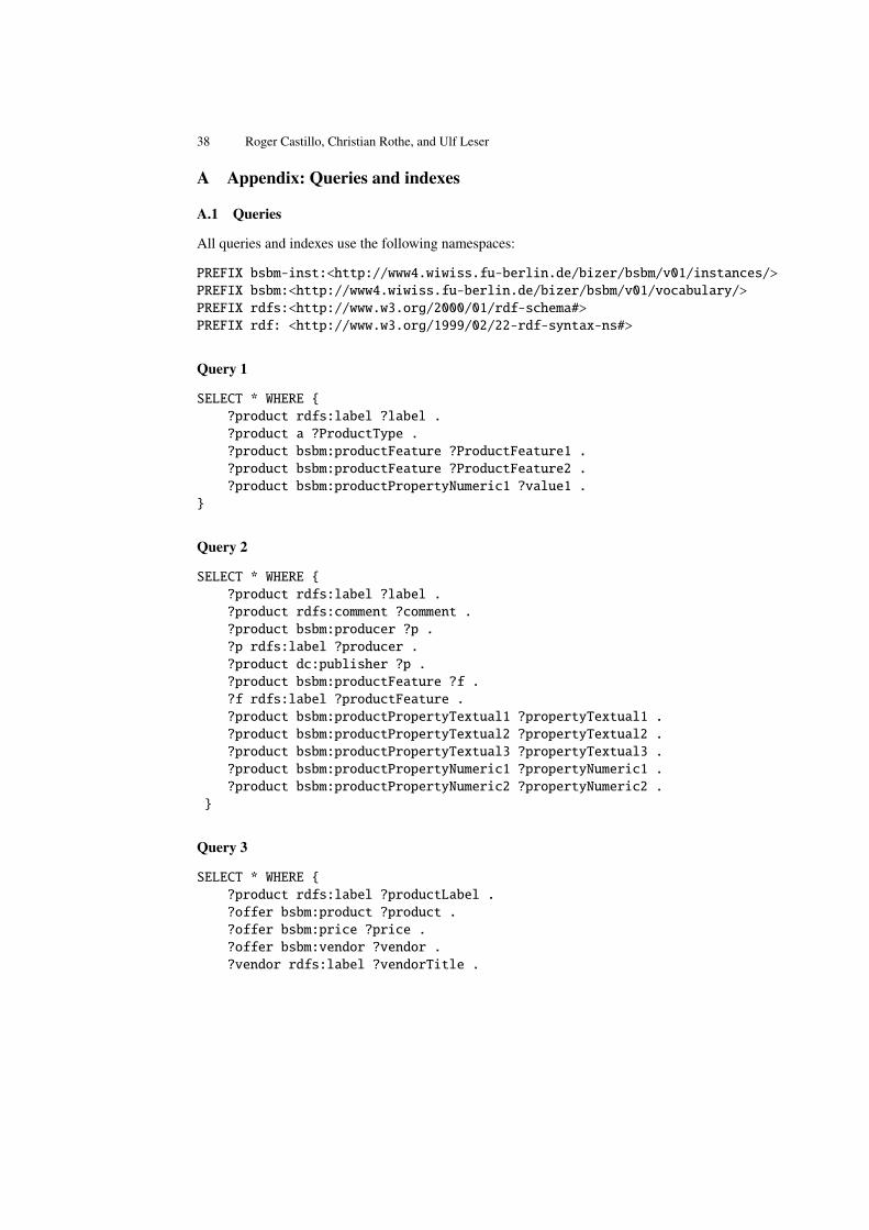
Our test queries are the following (see Appendix A.1 for full details):
– Query1: Finds a complete list of products with a set of generic features.– Query2: Retrieve all basic information related to the list of products.– Query3: Retrieve in-depth information about products including offers and reviews.
RDFMatView: Indexing RDF Data for SPARQL Queries 29
Fig. 9. Triple representation of the data set. Publisher and publication data are captured for eachinstance by a publisher and a date triple.
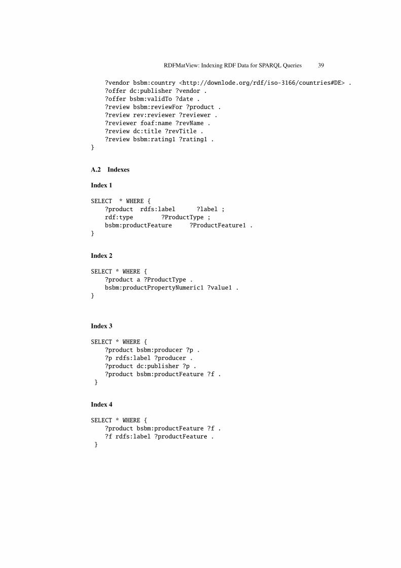
The query patterns contain 5, 12 and 13 triple patterns and 6, 12 and 12 differentvariables, respectively. Afterwards, based on the patterns of these queries, we generatea set of 10 indexes. Indexes are constructed such that they often lead to covers contain-ing a combination of indexes that do not cover the query entirely, since most real-lifeSPARQL queries fit this case. Indexes were derived using the following rules:
1. Indexes must be completely subsumed by at least one test queries.2. None of the indexes should completely cover any of the test queries (this case would
be trivial).3. Indexes should have different embeddings that should be intensionally overlapping.
The size of the index patterns varies from 2 to 9 triples. As an example, indexes inTable 10 were derived from Query1. Appendix A.2 gives a complete description of allindexes.
These indexes are designed not only to cover a part of the query, but also to generatemultiple embeddings in the query pattern by means of different mappings. The genera-tion of such embeddings allows us to measure the performance of the query processingwhen using the same participating indexes multiple times covering different parts of thequery pattern.
7.3 Experiments
In this section, we report the results of our experimental study with the data sets, queriesand indexes described in Section 7.2. We evaluated three queries on five different datasets using our three RDFMatView methods and plain ARQ (without indexes), whichamounts to 45 different configurations. In this section, we refer to the different ap-proaches to query execution as M1 for MatView-and-ARQ, M2 for MatView-to-SQL,
30 Roger Castillo, Christian Rothe, and Ulf Leser
Table 10. RDFMatView indexes derived from Query1.
Index1 : SELECT ∗ WHERE {? p r o d u c t r d f s : l a b e l ? l a b e l ;r d f : t y p e ? Produc tType ;bsbm : p r o d u c t F e a t u r e ? P r o d u c t F e a t u r e 1 . }
Index2 : SELECT ∗ WHERE {? p r o d u c t r d f : t y p e ? Produc tType ;bsbm : p r o d u c t P r o p e r t y N u m e r i c 1 ? v a l u e 1 . }
M3 for the hybrid approach, and ARQ for plain ARQ. We performed experiments usingthe optimal cover and also evaluated the real and estimated costs of different covers forthe same query. Optimal covers were selected according to Lemma 2 (see Section 5).All queries were executed 5 times and average execution times are reported.
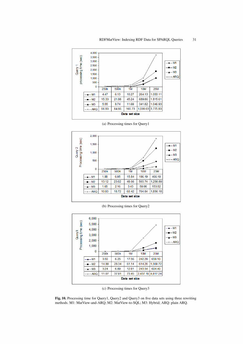
Figure 10 illustrates the average processing times for each of the 45 configurations.Clearly, processing time significantly improves when using MatView-and-ARQ (M1)and Hybrid (M3). The improvements are the higher, the larger the database. Processingtime does not improve significantly when using MatView-to-SQL (M2). The reason forthis is the Jena native storage schema (see Section 6.1). Since the values are encodedfollowing the Jena layout, our process needs to parse the stored values and extract therequired information. This process must be performed for each value associated to anexported variable of the query.
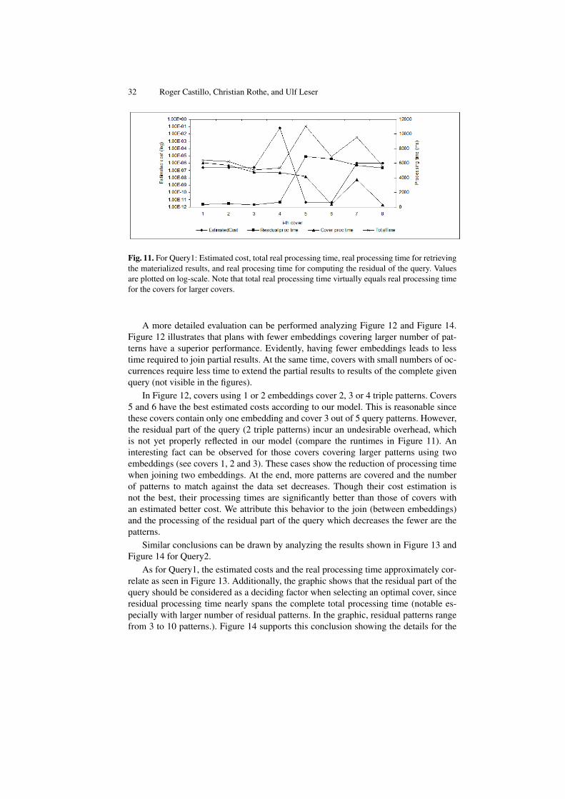
A comparison of real and estimated costs for different covers for Query1 and Query2are shown in Figure 11 and Figure 13, respectively. Additionally, we analyze in Figure12 and Figure 14 the relation between the estimated costs of a cover, the number of em-beddings it contains and the number of covered and uncovered query patterns. In thesefigures, covers are sorted descending order first by number of covered patterns, secondby number of participating embeddings and third by number of residual patterns. Thisordering allow us to verify the correlation between the estimated costs and the numberof covered patterns. It also evidences the influence of the number of participating em-beddings and residual patterns in the query processing time. Note that Cover 6 in Figure11 (for Query1) and cover 3 in Figure 13 (for Query2) are those that our system selectsas optimal.
Figure 11 and Figure 13 show that the costs estimated by our cost model roughlycorrelate with the real processing time. However, they also show that there is ampleroom for improvements. For instance, our model does not yet reflect that using less in-dexes is advantageous as this requires less joins at runtime; this fact is captured onlyindirectly by our model as we concentrate on the number of covered patterns. Neverthe-less, the results give evidence that our model helps in avoiding the usage of bad plans.Actually all plans improve the total execution times when compared to those withoutusing indexes.
RDFMatView: Indexing RDF Data for SPARQL Queries 31
(a) Processing times for Query1
(b) Processing times for Query2
(c) Processing times for Query3
Fig. 10. Processing time for Query1, Query2 and Query3 on five data sets using three rewritingmethods. M1: MatView-and-ARQ; M2: MatView-to-SQL; M3: Hybrid; ARQ: plain ARQ.
32 Roger Castillo, Christian Rothe, and Ulf Leser
Fig. 11. For Query1: Estimated cost, total real processing time, real processing time for retrievingthe materialized results, and real procesing time for computing the residual of the query. Valuesare plotted on log-scale. Note that total real processing time virtually equals real processing timefor the covers for larger covers.
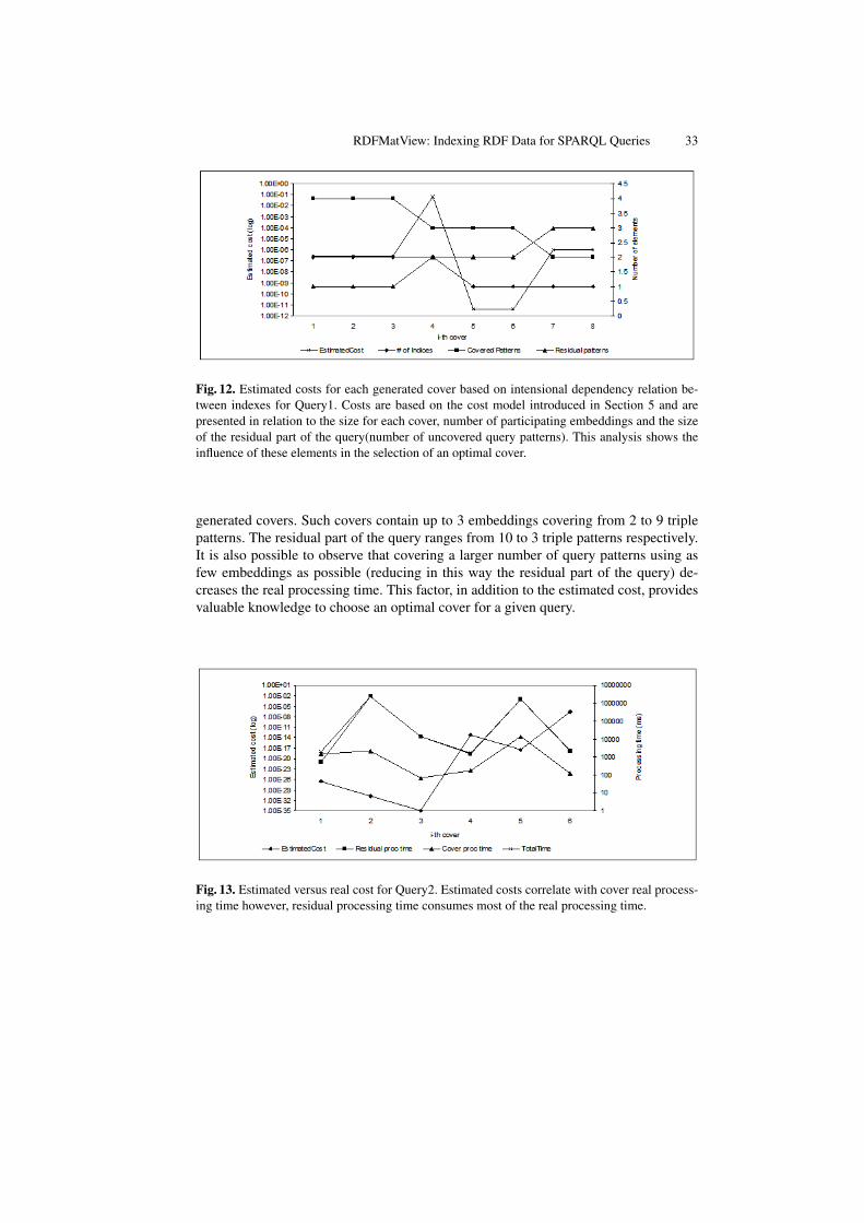
A more detailed evaluation can be performed analyzing Figure 12 and Figure 14.Figure 12 illustrates that plans with fewer embeddings covering larger number of pat-terns have a superior performance. Evidently, having fewer embeddings leads to lesstime required to join partial results. At the same time, covers with small numbers of oc-currences require less time to extend the partial results to results of the complete givenquery (not visible in the figures).
In Figure 12, covers using 1 or 2 embeddings cover 2, 3 or 4 triple patterns. Covers5 and 6 have the best estimated costs according to our model. This is reasonable sincethese covers contain only one embedding and cover 3 out of 5 query patterns. However,the residual part of the query (2 triple patterns) incur an undesirable overhead, whichis not yet properly reflected in our model (compare the runtimes in Figure 11). Aninteresting fact can be observed for those covers covering larger patterns using twoembeddings (see covers 1, 2 and 3). These cases show the reduction of processing timewhen joining two embeddings. At the end, more patterns are covered and the numberof patterns to match against the data set decreases. Though their cost estimation isnot the best, their processing times are significantly better than those of covers withan estimated better cost. We attribute this behavior to the join (between embeddings)and the processing of the residual part of the query which decreases the fewer are thepatterns.
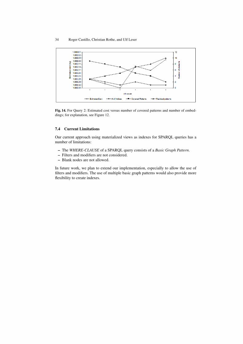
Similar conclusions can be drawn by analyzing the results shown in Figure 13 andFigure 14 for Query2.
As for Query1, the estimated costs and the real processing time approximately cor-relate as seen in Figure 13. Additionally, the graphic shows that the residual part of thequery should be considered as a deciding factor when selecting an optimal cover, sinceresidual processing time nearly spans the complete total processing time (notable es-pecially with larger number of residual patterns. In the graphic, residual patterns rangefrom 3 to 10 patterns.). Figure 14 supports this conclusion showing the details for the
RDFMatView: Indexing RDF Data for SPARQL Queries 33
Fig. 12. Estimated costs for each generated cover based on intensional dependency relation be-tween indexes for Query1. Costs are based on the cost model introduced in Section 5 and arepresented in relation to the size for each cover, number of participating embeddings and the sizeof the residual part of the query(number of uncovered query patterns). This analysis shows theinfluence of these elements in the selection of an optimal cover.
generated covers. Such covers contain up to 3 embeddings covering from 2 to 9 triplepatterns. The residual part of the query ranges from 10 to 3 triple patterns respectively.It is also possible to observe that covering a larger number of query patterns using asfew embeddings as possible (reducing in this way the residual part of the query) de-creases the real processing time. This factor, in addition to the estimated cost, providesvaluable knowledge to choose an optimal cover for a given query.
Fig. 13. Estimated versus real cost for Query2. Estimated costs correlate with cover real process-ing time however, residual processing time consumes most of the real processing time.
34 Roger Castillo, Christian Rothe, and Ulf Leser
Fig. 14. For Query 2: Estimated cost versus number of covered patterns and number of embed-dings; for explanation, see Figure 12.
7.4 Current Limitations
Our current approach using materialized views as indexes for SPARQL queries has anumber of limitations:
– The WHERE-CLAUSE of a SPARQL query consists of a Basic Graph Pattern.– Filters and modifiers are not considered.– Blank nodes are not allowed.
In future work, we plan to extend our implementation, especially to allow the use offilters and modifiers. The use of multiple basic graph patterns would also provide moreflexibility to create indexes.
RDFMatView: Indexing RDF Data for SPARQL Queries 35
8 Conclusions and future work
In this article we have proposed a novel method to speed-up the execution of SPARQLqueries. We introduced a logical and physical framework to answer a SPARQL queryusing materialized views as indexes. At runtime, queries are analyzed to see whetherthey can be executed by using one or more of those precomputed views. Experimentshave shown that the achievable performance gains are considerable. However, a closerlook also revealed that our cost model still can be improved. This, and the removal ofseveral technical limitations of our approach which restrict the types of queries it canhandle, will be the focus of our future work.
First, we defined an RDF data dictionary to identify all different resources. Second,we preprocessed SPARQL queries materializing the result sets. Our approach indexesnot only RDF data but proposes a native SPARQL index method. The use of RDF-MatView indexes minimizes query pattern comparison against the RDF data set. Weanalyze query and index patterns to generate all covers for a SPARQL query and alsothe rewriting of the latter to use indexes and get the final query result set. Even when theexecution time of our approach is higher than the execution time in ARQ, the processingtime significantly decreases using some strategies of our approach. It is important to no-tice that execution time of our approach remains constant and depends only on the sizeof the query pattern. Additionally, we analyzed and compared all generated covers. Ourresults show that besides the costs, the number of indexes and size of a cover, as well asthe residual query patterns are determining to select an optimal cover. We restrict ourapproach to execute queries containing only a basic graph pattern. In the future we willcontinue working on the optimization of the query processing analyzing other storageschemas as well as on the improvement of our algorithms for an optimal generation ofexecution plans using more complex queries. Another interesting and promising topicto extend our approach is index selection for SPARQL queries, i.e., given a workload ofSPARQL queries, perform a suggestion of which indexes should be built to efficientlyanswer these queries.
36 Roger Castillo, Christian Rothe, and Ulf Leser
References
1. Manola, F., Miller, E.: RDF Primer (February 2004) W3C Recommendation.2. Prud’hommeaux, E., Seaborne, A.: SPARQL Query Language for RDF (April 2008) W3C
Recommendation.3. Wilkinson, K., Sayers, C., Kuno, H., Reynolds, D.: Efficient RDF storage and retrieval in
Jena2. In: Proc. First International Workshop on Semantic Web and Databases. (2003)4. Stephen Harris, N.G.: 3store: Efficient bulk rdf storage. In: 1st International Workshop on
Practical and Scalable Semantic Systems (PSSS’03). (2003)5. Harris, S.: Sparql query processing with conventional relational database systems. In: Inter-
national Workshop on Scalable Semantic Web Knowledge Base System. (2005)6. Broekstra, J., Kampman, A., van Harmelen, F.: Sesame: A generic architecture for storing
and querying rdf and rdf schema. In: International Semantic Web Conference. (2002) 54–687. Dataset, U.R.: http://dev.isb-sib.ch/projects/uniprot-rdf/8. Project, W.S.C.: Linking open data on the semantic web.
http://esw.w3.org/topic/sweoig/taskforces/communityprojects/linkingopendata/
9. Bio2RDF. http://bio2rdf.org/ (2009)10. Heese, R., Leser, U., Quilitz, B., Rothe, C.: Index support for sparql. European Semantic
Web Conference, Innsbruck, Austria (2007)11. Abadi, D.J., Marcus, A., Madden, S.R., Hollenbach, K.: Scalable semantic web data man-
agement using vertical partitioning. In: VLDB ’07: Proceedings of the 33rd internationalconference on Very large data bases, VLDB Endowment (2007) 411–422
12. Weiss, C., Karras, P., Bernstein, A.: Hexastore: sextuple indexing for semantic web datamanagement. Proc. VLDB Endow. 1(1) (2008) 1008–1019
13. Neumann, T., Weikum, G.: Rdf-3x: a risc-style engine for rdf. Proc. VLDB Endow. 1(1)(2008) 647–659
14. Udrea, O., Pugliese, A., Subrahmanian, V.S.: Grin: A graph based rdf index. In: AAAI.(2007) 1465–1470
15. Groppe, S., Groppe, J., Linnemann, V.: Using an Index of Precomputed Joins in order tospeed up SPARQL Processing. In Cardoso, J., Cordeiro, J., Filipe, J., eds.: Proceedings9th International Conference on Enterprise Information Systems (ICEIS 2007 (1), VolumeDISI), Funchal, Madeira, Portugal, INSTICC (June 12 - 16 2007) 13–20
16. Connolly, T.M., Begg, C.E., Strachan, A.D.: Database systems: a practical approach to de-sign, implementation and management. Addison Wesley Longman Publishing Co., Inc.,Redwood City, CA, USA (1996)
17. Halevy, A.Y.: Answering queries using views: A survey. The VLDB Journal 10(4) (2001)270–294
18. Patrick Hayes, B.M.: Rdf semantics (February 2004) W3C Recommendation.19. ARQJena: Arq - a sparql processor for jena. http://jena.sourceforge.net/ARQ/ (2010)20. Chebotko, A., Lu, S., Jamil, H.M., Fotouhi, F.: Semantics preserving sparql-to-sql query
translation for optional graph patterns. Technical report, Department of Computer Science,Wayne State University (2006)
21. Bizer, C., Schultz, A.: The berlin sparql benchmark. International Journal On Semantic Weband Information Systems - Special Issue on Scalability and Performance of Semantic WebSystems, 2009 (2009)
22. Comer, D.: The difficulty of optimum index selection. ACM Trans. Database Syst. 3(4)(1978) 440–445
23. Caprara, A., Fischetti, M., Maio, D.: Exact and approximate algorithms for the index se-lection problem in physical database design. IEEE Transactions on Knowledge and DataEngineering 7(6) (1995) 955–967

RDFMatView: Indexing RDF Data for SPARQL Queries 37
24. Chaudhuri, S., Narasayya, V.R.: An efficient cost-driven index selection tool for microsoftsql server. In: VLDB ’97: Proceedings of the 23rd International Conference on Very LargeData Bases, San Francisco, CA, USA, Morgan Kaufmann Publishers Inc. (1997) 146–155
38 Roger Castillo, Christian Rothe, and Ulf Leser
A Appendix: Queries and indexes
A.1 Queries
All queries and indexes use the following namespaces:
PREFIX bsbm-inst:<http://www4.wiwiss.fu-berlin.de/bizer/bsbm/v01/instances/>
PREFIX bsbm:<http://www4.wiwiss.fu-berlin.de/bizer/bsbm/v01/vocabulary/>
PREFIX rdfs:<http://www.w3.org/2000/01/rdf-schema#>
PREFIX rdf: <http://www.w3.org/1999/02/22-rdf-syntax-ns#>
Query 1
SELECT * WHERE {
?product rdfs:label ?label .
?product a ?ProductType .
?product bsbm:productFeature ?ProductFeature1 .
?product bsbm:productFeature ?ProductFeature2 .
?product bsbm:productPropertyNumeric1 ?value1 .
}
Query 2
SELECT * WHERE {
?product rdfs:label ?label .
?product rdfs:comment ?comment .
?product bsbm:producer ?p .
?p rdfs:label ?producer .
?product dc:publisher ?p .
?product bsbm:productFeature ?f .
?f rdfs:label ?productFeature .
?product bsbm:productPropertyTextual1 ?propertyTextual1 .
?product bsbm:productPropertyTextual2 ?propertyTextual2 .
?product bsbm:productPropertyTextual3 ?propertyTextual3 .
?product bsbm:productPropertyNumeric1 ?propertyNumeric1 .
?product bsbm:productPropertyNumeric2 ?propertyNumeric2 .
}
Query 3
SELECT * WHERE {
?product rdfs:label ?productLabel .
?offer bsbm:product ?product .
?offer bsbm:price ?price .
?offer bsbm:vendor ?vendor .
?vendor rdfs:label ?vendorTitle .
RDFMatView: Indexing RDF Data for SPARQL Queries 39
?vendor bsbm:country <http://downlode.org/rdf/iso-3166/countries#DE> .
?offer dc:publisher ?vendor .
?offer bsbm:validTo ?date .
?review bsbm:reviewFor ?product .
?review rev:reviewer ?reviewer .
?reviewer foaf:name ?revName .
?review dc:title ?revTitle .
?review bsbm:rating1 ?rating1 .
}
A.2 Indexes
Index 1
SELECT * WHERE {
?product rdfs:label ?label ;
rdf:type ?ProductType ;
bsbm:productFeature ?ProductFeature1 .
}
Index 2
SELECT * WHERE {
?product a ?ProductType .
bsbm:productPropertyNumeric1 ?value1 .
}
Index 3
SELECT * WHERE {
?product bsbm:producer ?p .
?p rdfs:label ?producer .
?product dc:publisher ?p .
?product bsbm:productFeature ?f .
}
Index 4
SELECT * WHERE {
?product bsbm:productFeature ?f .
?f rdfs:label ?productFeature .
}
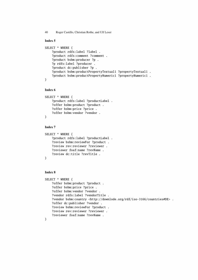
40 Roger Castillo, Christian Rothe, and Ulf Leser
Index 5
SELECT * WHERE {
?product rdfs:label ?label .
?product rdfs:comment ?comment .
?product bsbm:producer ?p .
?p rdfs:label ?producer .
?product dc:publisher ?p .
?product bsbm:productPropertyTextual1 ?propertyTextual1 .
?product bsbm:productPropertyNumeric1 ?propertyNumeric1 .
}
Index 6
SELECT * WHERE {
?product rdfs:label ?productLabel .
?offer bsbm:product ?product .
?offer bsbm:price ?price .
?offer bsbm:vendor ?vendor .
}
Index 7
SELECT * WHERE {
?product rdfs:label ?productLabel .
?review bsbm:reviewFor ?product .
?review rev:reviewer ?reviewer .
?reviewer foaf:name ?revName .
?review dc:title ?revTitle .
}
Index 8
SELECT * WHERE {
?offer bsbm:product ?product .
?offer bsbm:price ?price .
?offer bsbm:vendor ?vendor .
?vendor rdfs:label ?vendorTitle .
?vendor bsbm:country <http://downlode.org/rdf/iso-3166/countries#DE> .
?offer dc:publisher ?vendor .
?review bsbm:reviewFor ?product .
?review rev:reviewer ?reviewer .
?reviewer foaf:name ?revName .
}
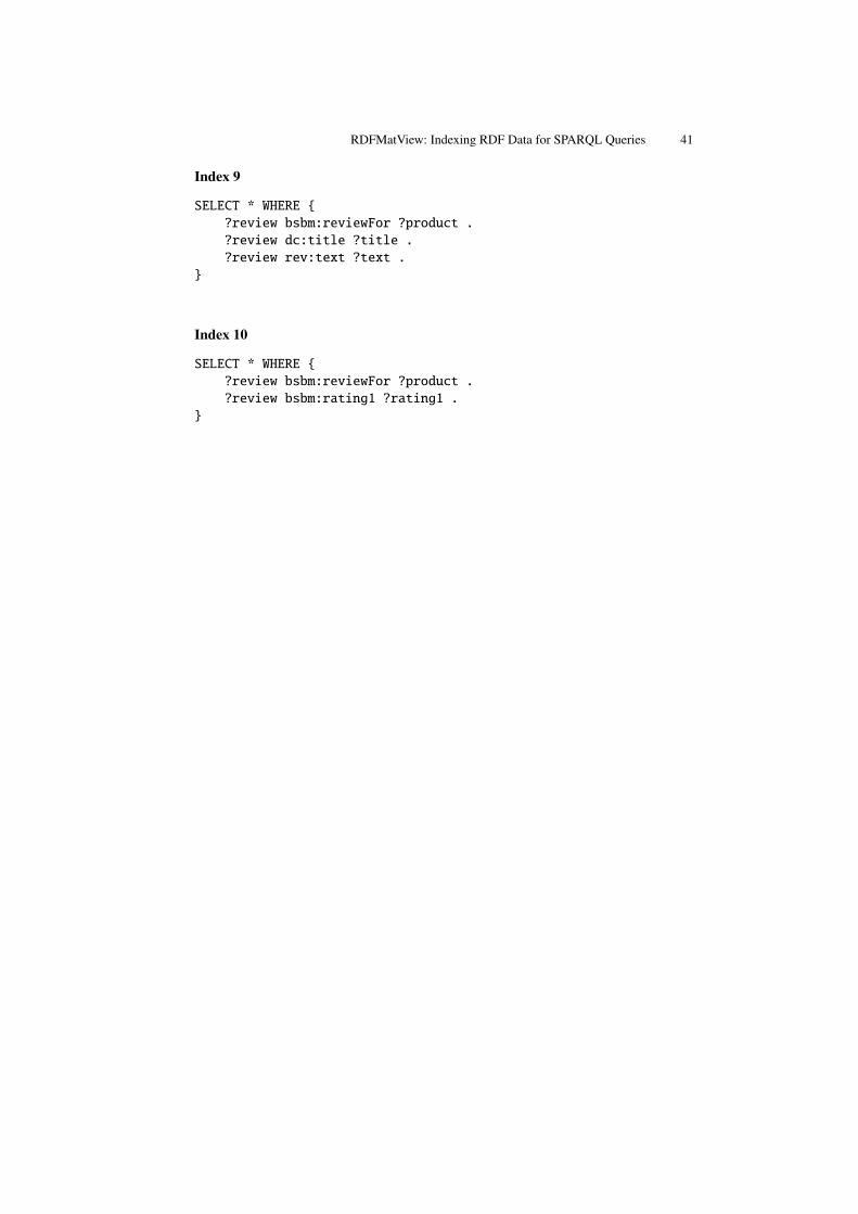
RDFMatView: Indexing RDF Data for SPARQL Queries 41
Index 9
SELECT * WHERE {
?review bsbm:reviewFor ?product .
?review dc:title ?title .
?review rev:text ?text .
}
Index 10
SELECT * WHERE {
?review bsbm:reviewFor ?product .
?review bsbm:rating1 ?rating1 .
}