R&D Report Research - Methods - Development 1998:3

On the Stratification of Highly Skewed Populations (Dan Hedlin)

This thesis was originally published as report No. B:41, 1998, of the Institute of Actuarial Mathematics and Mathematical Statistics and is reprinted here after kind permission by the University of Stockholm. Statistics Sweden 1998

Från trycket Ansvarig utgivare Producent

Maj 1998 Lars Lyberg Statistiska centralbyrån, utvecklingsavdelningen

Förfrågningar Dan Hedlin e-post dhl @ socsci.soton.ac.uk

© 1998, Statistiska centralbyrån

ISSN 0283-8680 Printed in Sweden

R & D Report 1998:3. On the stratification of highly skewed population / Dan Hedlin. Digitaliserad av Statistiska centralbyrån (SCB) 2016. urn:nbn:se:scb-1998-X101OP9803

INLEDNING

TILL

R & D report : research, methods, development / Statistics Sweden. – Stockholm :

Statistiska centralbyrån, 1988-2004. – Nr. 1988:1-2004:2.

Häri ingår Abstracts : sammanfattningar av metodrapporter från SCB med egen

numrering.

Föregångare:

Metodinformation : preliminär rapport från Statistiska centralbyrån. – Stockholm :

Statistiska centralbyrån. – 1984-1986. – Nr 1984:1-1986:8.

U/ADB / Statistics Sweden. – Stockholm : Statistiska centralbyrån, 1986-1987. – Nr E24-

E26

R & D report : research, methods, development, U/STM / Statistics Sweden. – Stockholm :

Statistiska centralbyrån, 1987. – Nr 29-41.

Efterföljare:

Research and development : methodology reports from Statistics Sweden. – Stockholm :

Statistiska centralbyrån. – 2006-. – Nr 2006:1-.

R&D Report Research - Methods - Development 1998:3

On the Stratification of

Highly Skewed Populations

Dan Hedlin

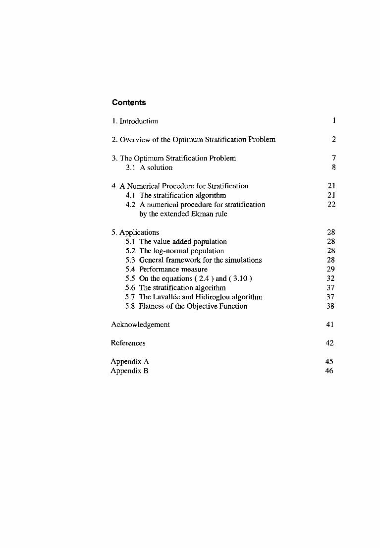
Contents

1. Introduction 1

2. Overview of the Optimum Stratification Problem 2

3. The Optimum Stratification Problem 7 3.1 A solution 8

4. A Numerical Procedure for Stratification 21 4.1 The stratification algorithm 21 4.2 A numerical procedure for stratification

by the extended Ekman rule 22

5. Applications 28 5.1 The value added population 28 5.2 The log-normal population 28 5.3 General framework for the simulations 28 5.4 Performance measure 29 5.5 On the equations (2 .4) and (3.10) 32 5.6 The stratification algorithm 37 5.7 The Lavallée and Hidiroglou algorithm 37 5.8 Flatness of the Objective Function 38

Acknowledgement 41

References 42

Appendix A 45 Appendix B 46

Abstract

This paper discusses the problem of stratifying highly skewed populations, such as those encountered in many business surveys. We give conditions which must be satisfied for stratum boundaries to minimize the variance of the standard estimator of the population total. The paper appears to be the first one that deals with the combined problem of allocation and stratification in order to minimize the variance of the usual unbiased estimator, taking into account that the population is finite. The proof utilizes the Kuhn-Tucker Theorem. An iterative numerical method for practical application of the analytic results is proposed.

1 Introduction

Stratification is a widely used sample survey technique. The sampling frame is divided into strata and independent samples are drawn from the strata. There are a number of reasons for stratification. It is common in business surveys, for example, to use slightly different questionnaires for different subpopulations. Then it is natural to let each subpopulation be a stratum.

For the purpose of bringing estimator variances down there are two main types of beneficial stratifications:

(1) The survey designer forms strata as close to important study domains as possible, which will allow him to control sample sizes in strata and thereby the precision of domain statistics. We refer to these strata as pre-strata.

(2) The survey designer forms homogenized strata, which are obtained if important study variables vary less within strata than in the unstratified population (or in the pre-stratum). Such stratification is typically carried out as follows. Strata are formed by classifying the values of a stratification variable available in the sampling frame. Such a stratification increases the precision of the resulting statistics in cases where the stratification variable and the study variable are fairly strongly correlated. The effect of increasing precision is particularly strong when the study variables have highly skewed distributions, which is usually the case in business surveys. Then, typically, the stratum with the largest businesses is a self-representing stratum (also called "certainty stratum" or "take-all stratum") where all businesses are selected for observation.

In the sequel we will focus on objective (2).

Several problems have to be addressed when designing a stratified sample. The following list is taken from Särndal, Swensson and Wretman (1992) with some modification.

1

Construction of Strata Al. Which stratification variable(s) is (are) to be used? A2. How many strata should there be? A3. How should strata be demarcated?

Choice of Sampling and Estimation Methods within Strata Bl. Sampling design for each stratum B2. An estimator for each stratum B3. The sample size for each stratum

Often the same type of design and estimator are used for all strata.

This paper focuses on questions A3 and B3 jointly, under the assumptions that the stratification variable is equal to the study variable. Section 2 gives an overview of the literature in this field and section 3 states conditions for stratum boundaries minimizing the variance. In section 4 an iterative numerical algorithm for univariate stratification of highly skewed populations is put forward. Applications are presented in section 5.

2 Overview of the Optimum Stratification Problem

There are a number of the problems associated with stratum construction in highly skewed populations. Sigman and Monsour (1995) give an overview.

The main problem to be considered in this report is: How should strata be demarcated? There is a considerable literature on optimal stratification for the usual unbiased estimator. In this section we give an overview of the most important references addressing this question in the context of homogenized strata. First we formulate some assumptions and approaches common in this literature.

This problem is usually treated as a "single-purpose" one in that just one parameter is considered. The following problem may be called the common optimum stratification problem. This is the problem, with slight modifications in some cases, that most of the literature on this subject as well as this report discuss. Consider the standard estimator of the total of a study variable y:

(2.1)

The problem is to find the stratification that minimizes the variance of t,

(2.2)

where Nh and «/, are the number of frame units in stratum h and the sample

2

size in stratum h, respectively, and sjh is the study variable variance in

stratum h,

where yh is the study variable mean in stratum h. Nh, S2yh and yh are

functions of the stratum boundaries. The number of strata, H, is fixed but arbitrary. A simple random sample is drawn from each stratum. The total sample size n = n{ +n2+...+nH is fixed.

It is well known that Neyman allocation gives the optimal sample sizes within strata, in the sense that the variance of f is minimized. If nothing else is stated the articles referred to in this section use Neyman allocation. Some authors, however, prefer other allocation schemes, thus deviating slightly from the optimum solution.

We will refer to a stratum where a frame unit is sampled with a probability less than one as a genuine sampling stratum as opposed to a certainty stratum where all frame units are included in the sample.

Either of the two following assumptions is widely used in connection with the common optimum stratification problem. Both are associated with the choice of stratification variable, problem Al. In this paper, we work under assumption Al.a only.

Assumption Al.a The values of a single auxiliary variable are known and it is, although unrealistically, assumed that the values of study variables equal those of the stratification variable.

Assumption Al.b The values of a single auxiliary variable are known and some stochastic relationship between the study variable and the stratification variable is assumed.

Many articles draw on the following approximation.

Approximation 1 The finite population correction is ignored when minimizing the estimator variance.

Comment: while the finite population correction is negligible in many practical applications, approximation 1 is crude if it used for a certainty stratum as this means replacing a zero variance with a strictly positive one for that stratum. Consequently, approximation 1 is questionable for highly skewed populations.

The approaches used to address the common optimum stratification

3

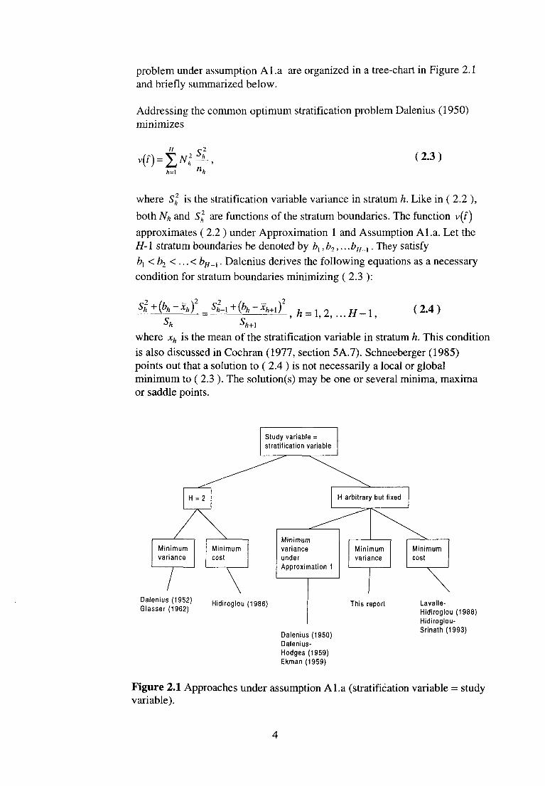
problem under assumption Al.a are organized in a tree-chart in Figure 2.1 and briefly summarized below.

Addressing the common optimum stratification problem Dalenius (1950) minimizes

(2.3)

where 5A2 is the stratification variable variance in stratum h. Like in ( 2.2 ),

both Nh and si are functions of the stratum boundaries. The function v(f)

approximates ( 2.2 ) under Approximation 1 and Assumption A l.a. Let the H-1 stratum boundaries be denoted by b{,b2,...&#_,. They satisfy bx <b2 < ...< bH_{. Dalenius derives the following equations as a necessary condition for stratum boundaries minimizing ( 2.3 ):

(2.4)

where xh is the mean of the stratification variable in stratum h. This condition is also discussed in Cochran (1977, section 5A.7). Schneeberger (1985) points out that a solution to ( 2.4 ) is not necessarily a local or global minimum to ( 2.3 ). The solution(s) may be one or several minima, maxima or saddle points.

Figure 2.1 Approaches under assumption A l.a (stratification variable = study variable).

4

The Dalenius equations ( 2.4 ) are, however, ill adapted to practical computation. Consequently, a large number of approximate methods for constructing genuine sampling strata have been suggested. The most efficient from a precision-increasing point of view are presumably the Dalenius-Hodges rule ("the cum -JJrule") and the Ekman rule (Dalenius, Hodges

(1959); Ekman (1959); Cochran (1961); Hess et al. (1966) and Murthy (1967)). A numerical procedure for the Ekman rule is presented in section 4 of this report. Both the Dalenius-Hodges rule and the Ekman rule give approximate solutions to the Dalenius equations ( 2.4 ). Since no stratum is allowed to be a certainty stratum these boundaries are not optimal for highly skewed populations.

Several authors have addressed the problem of finding the point where the far tail of a skewed distribution should be cut off to form a certainty stratum. All elements in the certainty stratum are included in the sample. None of the papers mentioned below, all of which consider designs that include a certainty stratum, draw on Approximation 1. Several solutions have been proposed to the special case of this problem when the population is divided into two strata only, one certainty stratum and one genuine sampling stratum. In this special case Dalenius (1952) suggests a condition for the certainty stratum. Glasser (1962) derives an exact result, as opposed to Dalenius who approximates the finite population with an infinite population. Nevertheless, the Glasser equation for stratum boundary b\ is essentially equivalent with that of Dalenius:

(2.5)

where index 1 refers to stratum 1, which is the genuine sampling stratum.

Whereas Dalenius and Glasser make estimator precision as good as possible under given total sample size, Hidiroglou (1986) minimizes sample size under prescribed estimator precision. Like Dalenius and Glasser he works under assumption A La. Moreover, he too limits the number of strata to two, thus also limiting the practical usefulness of the results. The approaches of Dalenius, Glasser and Hidiroglou are not easily generalized to a number of strata greater than two.

The approach of this paper differs from the ones mentioned above in that here we address the combined problem of finding the optimal allocation and optimal stratification when there are several genuine sampling strata and one certainty stratum. Condition ( 2.5 ) is a special case of the results of this report, whereas ( 2.4 ) is not. The reason for this is that approximation 1 is not invoked in this report.

Next, we briefly describe an algorithm by Lavallée and Hidiroglou (1988) and Hidiroglou and Srinath (1993), both of which provide stratum boundaries for one certainty stratum and several genuine sample strata. Both papers address the common optimum stratification problem under assumption A La,

5

however, like in Hidiroglou (1986) the sample size is minimized under a precision constraint rather than the other way around. Hidiroglou and Lavallée use a form of power allocation of the sample:

where index h indicates stratum h and n, N and x are sample sizes, frame sizes and the mean of the stratification variable, respectively (a description of power allocation is provided by Särndal, Swensson and Wretman (1992)). Strata 1, 2,... H-1 are genuine sampling strata and stratum H is a certainty stratum with nH - N H. Hidiroglou and Srinath use a general allocation formula comprising several schemes, e g Neyman allocation. The stratum containing the largest units is predetermined to be a certainty stratum, the other strata to be genuine sampling strata. The iterative search algorithm finds the minimum of the objective function, which is the sample size viewed as a function of the stratum boundaries.

Sweet and Sigman (1995 b), Slanta and Krenzke (1996) and Detlefsen and Veum (1991) report on applications of the Lavallée and Hidiroglou algorithm. They found that the resulting boundaries depend on where the initial boundaries are set. Moreover, the convergence may be slow or non­existent. These findings made Detlefsen and Veum abandon the algorithm. Slanta and Krenzke studied the convergence of the algorithm applied to two populations. They propose ways of resolving difficulties with the algorithm, which they applied to one stratification variable of the Annual Capital Expenditures Survey at the US Bureau of the Census.

The approach of this report differs from that of Lavallée, Hidiroglou (1988) and Hidiroglou, Srinath (1993) in that here the estimator variance is treated as a function of the stratum boundaries and sample sizes within strata. The estimator variance is minimized under a fixed size of the total sample. The cited papers, however, solve a slightly different problem: the total sample size is seen as a function of the stratum boundaries. It is minimized under a predetermined estimator variance constraint. When the minimum size of the total sample is found, one part of the sample is allocated to the certainty stratum, and the remaining part is allocated to the genuine sampling strata according to a predetermined scheme, for example power allocation.

6

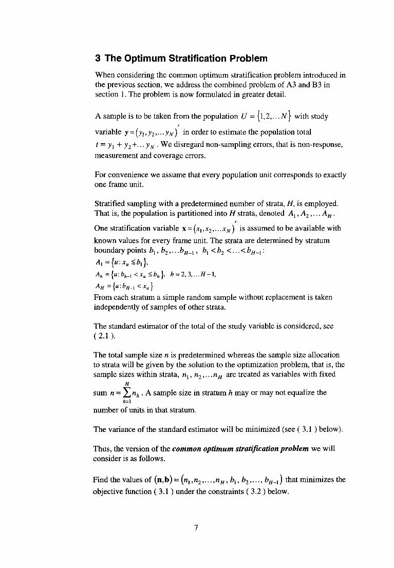
3 The Optimum Stratification Problem

When considering the common optimum stratification problem introduced in the previous section, we address the combined problem of A3 and B3 in section 1. The problem is now formulated in greater detail.

A sample is to be taken from the population U = {l,2,... N\ with study

variable y = (yx, y2,... yN ) in order to estimate the population total

t = y, + y2+... yN . We disregard non-sampling errors, that is non-response, measurement and coverage errors.

For convenience we assume that every population unit corresponds to exactly one frame unit.

Stratified sampling with a predetermined number of strata, H, is employed. That is, the population is partitioned into H strata, denoted Al,A2,...AH.

One stratification variable x = (jtj,x2,.. .xN ) is assumed to be available with

known values for every frame unit. The strata are determined by stratum boundary points bx,b2,...bH_x, bx<b2<...<bH_x :

From each stratum a simple random sample without replacement is taken independently of samples of other strata.

The standard estimator of the total of the study variable is considered, see (2.1).

The total sample size n is predetermined whereas the sample size allocation to strata will be given by the solution to the optimization problem, that is, the sample sizes within strata, nx, n2,...nH are treated as variables with fixed

H

sum n = 2^nh . A sample size in stratum h may or may not equalize the h=\

number of units in that stratum.

The variance of the standard estimator will be minimized (see ( 3.1 ) below).

Thus, the version of the common optimum stratification problem we will consider is as follows.

Find the values of (n,b) = (n,, n2,...,nH, bx, b2,..., bH_x ) that minimizes the

objective function ( 3.1 ) under the constraints ( 3.2 ) below.

7

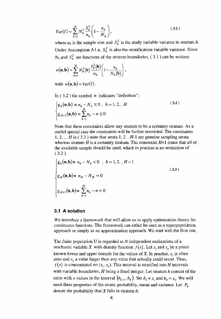
(3 .1)

where nh is the sample size and Si is the study variable variance in stratum h.

Under Assumption Al.a, S% is also the stratification variable variance. Since

Nh and Si are functions of the stratum boundaries, (3.1) can be written:

In ( 3.2 ) the symbol = indicates "definition":

(3.2)

Note that these constraints allow any stratum to be a certainty stratum. As a useful special case the constraints will be further restricted. The constraints 1, 2,... H in ( 3.3 ) state that strata 1, 2 ...H-\ are genuine sampling strata whereas stratum H is a certainty stratum. The constraint H+\ states that all of the available sample should be used, which in practise is no restriction of ( 3.2 ).

(3.3)

3.1 A solution

We introduce a framework that will allow us to apply optimization theory for continuous functions. The framework can either be seen as a superpopulation approach or simply as an approximation approach. We start with the first one.

The finite population U is regarded as N independent realizations of a stochastic variable X with density function f(x). Let JC, and xN be a priori

known lower and upper bounds for the values of X. In practise, x, is often zero and xN a value larger than any value that actually could occur. Thus, /(x) is concentrated on (x,, xN). This interval is stratified into H intervals

with variable boundaries, H being a fixed integer. Let stratum h consist of the

units with x-values in the interval \bh_x ,bhj. Set b0 = JC, and bH = xN. We will

need three properties of the strata: probability, mean and variance. Let Ph

denote the probability that X falls in stratum h:

8

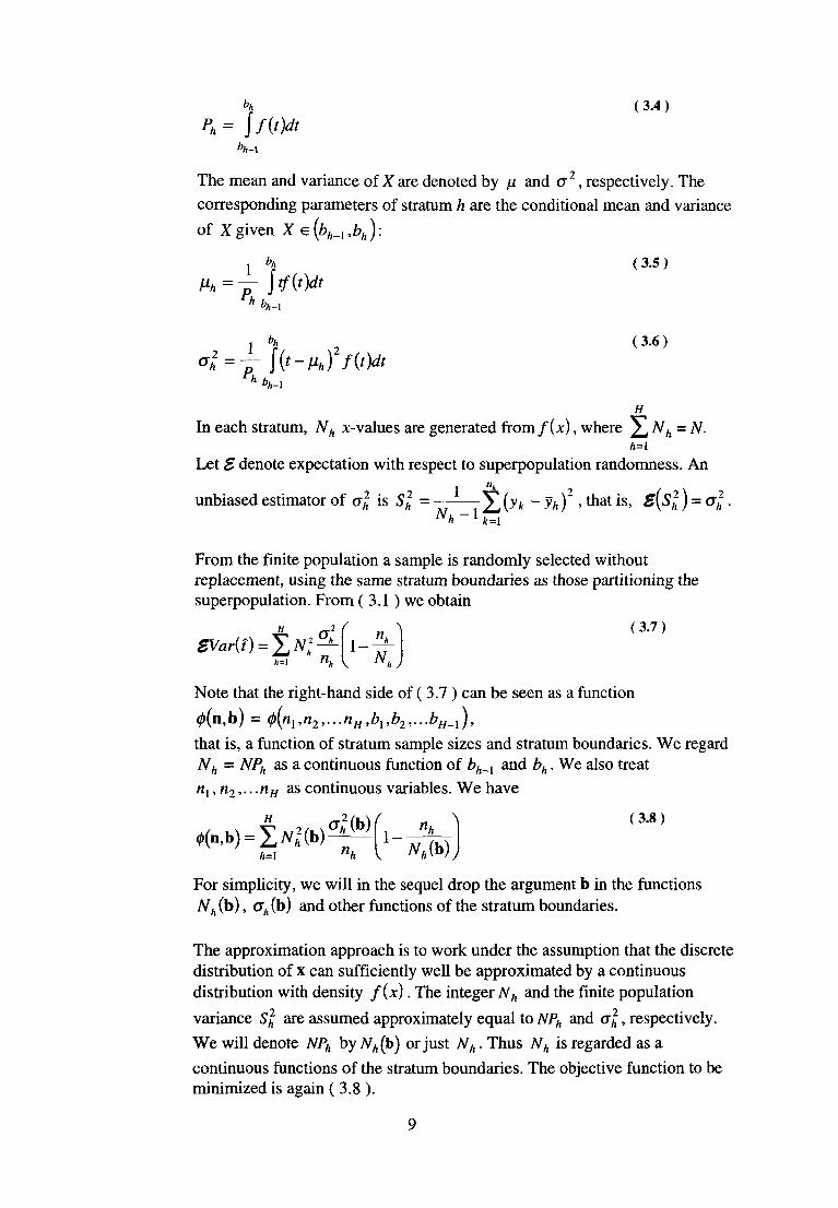
(3.4)

The mean and variance of X are denoted by \i and a1, respectively. The

corresponding parameters of stratum h are the conditional mean and variance

of Xgiven X e (£ A _iA) :

(3.5)

(3.6)

H

In each stratum, Nh jc-values are generated from/(jc), where 2^Nh = N.

Let £ denote expectation with respect to superpopulation randomness. An i "h

unbiased estimator of G\ is S\ = V (yk - yh ) , that is, S\Sl )-G^.

From the finite population a sample is randomly selected without replacement, using the same stratum boundaries as those partitioning the superpopulation. From ( 3.1 ) we obtain

(3.7)

Note that the right-hand side of ( 3.7 ) can be seen as a function

that is, a function of stratum sample sizes and stratum boundaries. We regard Nh = NPh as a continuous function of bh_{ and bh. We also treat nx,n2,...nH as continuous variables. We have

(3.8)

For simplicity, we will in the sequel drop the argument b in the functions Nh (b), ah (b) and other functions of the stratum boundaries.

The approximation approach is to work under the assumption that the discrete distribution of x can sufficiently well be approximated by a continuous distribution with density f(x). The integer Nh and the finite population variance si are assumed approximately equal to NPh and al, respectively.

We will denote NPh by NA(b) or just Nh. Thus Nh is regarded as a

continuous functions of the stratum boundaries. The objective function to be minimized is again ( 3.8 ).

9

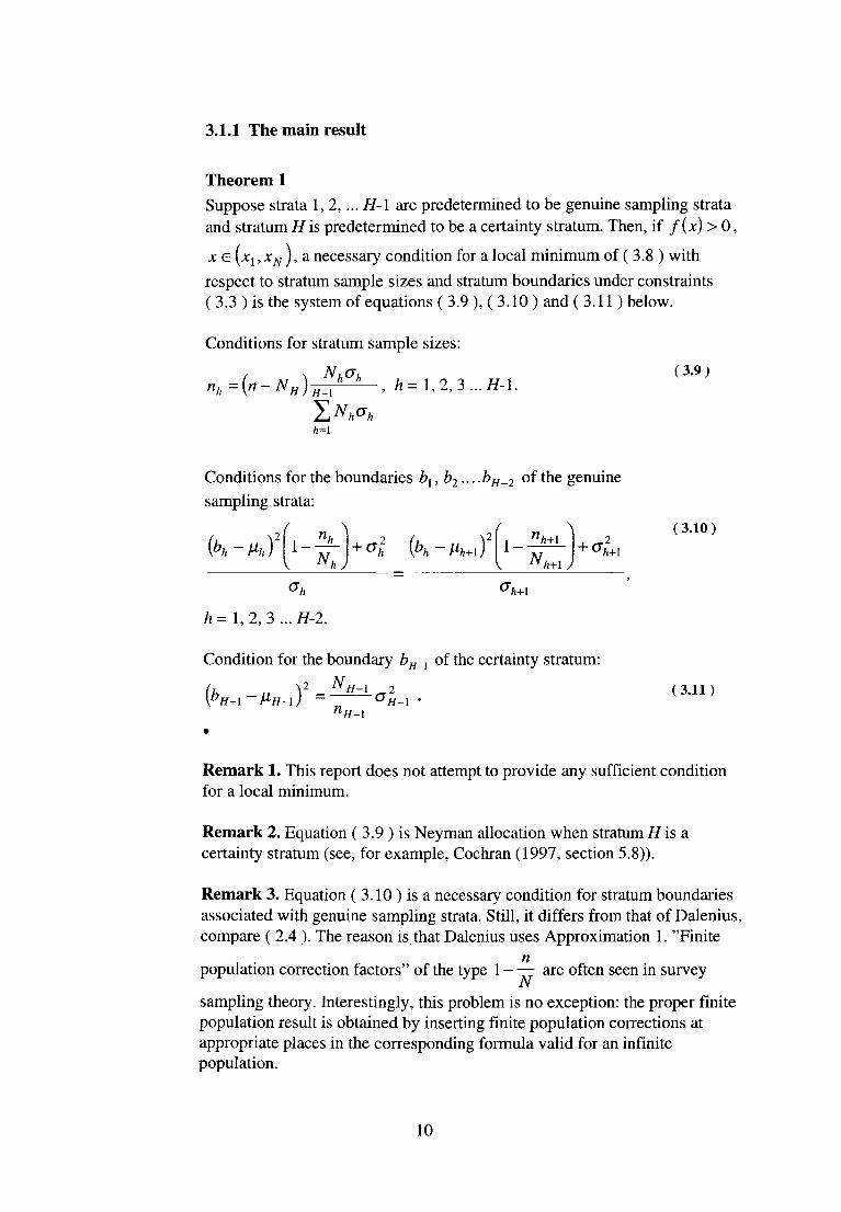
3.1.1 The main result

Theorem 1 Suppose strata 1, 2,... H-\ are predetermined to be genuine sampling strata and stratum H is predetermined to be a certainty stratum. Then, if f(x) > 0,

JC £ {xx ,xN ), a necessary condition for a local minimum of ( 3.8 ) with

respect to stratum sample sizes and stratum boundaries under constraints ( 3.3 ) is the system of equations ( 3.9 ), ( 3.10 ) and (3.11) below.

Conditions for stratum sample sizes:

(3.9)

Conditions for the boundaries b{, b2,...bH_2 of the genuine sampling strata:

(3.10)

Condition for the boundary bH_x of the certainty stratum:

( 3.11 )

Remark 1. This report does not attempt to provide any sufficient condition for a local minimum.

Remark 2. Equation ( 3.9 ) is Neyman allocation when stratum H is a certainty stratum (see, for example, Cochran (1997, section 5.8)).

Remark 3. Equation ( 3.10 ) is a necessary condition for stratum boundaries associated with genuine sampling strata. Still, it differs from that of Dalenius, compare ( 2.4 ). The reason is.that Dalenius uses Approximation 1. "Finite

n population correction factors" of the type 1 - — are often seen in survey

sampling theory. Interestingly, this problem is no exception: the proper finite population result is obtained by inserting finite population corrections at appropriate places in the corresponding formula valid for an infinite population.

10

Remark 4. For H = 2, equation ( 3.11 ) is equivalent to the condition of Glasser, see ( 2.5 ).

Remark 5. When applying Theorem 1 in a practical situation, the unknown superpopulation parameters nh and ol must be estimated or guessed by the corresponding parameters of the finite population. Moreover, in a practical situation the values of nh and Nh have to be rounded to nearest integer.

3.1.2 Auxiliary results

We will use the Kuhn-Tucker Theorem which provides necessary conditions for a local optimum of a function given certain constraints. For convenience the theorem is restated in Proposition 1. Definition 1 introduces the concept of a regular point that will be needed in Proposition 1. See for example Luenberger (1973) for a more detailed account.

Definition 1 Let (n,b) be a point satisfying the constraints

and

and let "H be the set of indices j for which ey (n,b) = 0. Then (n,b) is a

regular point of the constraints, if the gradient vectors

are linearly independent.

Note that the constraints ( 3.2 ) are of the form ei (n, b) < 0, j = 1, 2... H +1

while the two last constraints of ( 3.3 ) can be written di (n,b) = 0,

i = H,H + l.

Proposition 1 Denote the gradient vector of 0(n,b) by

Let (n ,b j be a local minimum for the problem of mimizing 0(n,b) subject

to the constraints

11

and suppose (n ,b j is a regular point of the constraints. Then there is a

vector v e R7 , with / real-valued components, and a vector A e R J with

A > 0 such that

(3.12)

(3.13)

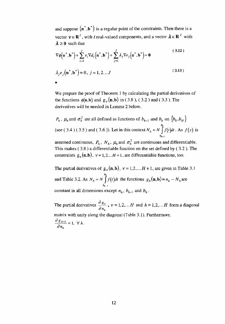
We prepare the proof of Theorem 1 by calculating the partial derivatives of

the functions 0(n,b) and gv(n,b) in ( 3.8 ), ( 3.2 ) and ( 3.3 ). The

derivatives will be needed in Lemma 2 below.

Ph, \ih and ol are all defined as functions of bh_x and bh on \b0,bH}

(see ( 3.4 ) ( 3.5 ) and ( 3.6 )). Let in this context Nh

assumed continuous, Ph, Nh, jihand a\ are continuous and differentiable. This makes ( 3.8 ) a differentiable function on the set defined by ( 3.2 ). The constraints gv (n,b), v = 1,2... H +1, are differentiable functions, too.

The partial derivatives of gv(n,b), v = \,2,...H+ 1, are given in Table 3.1 h

and Table 3.2. As Nh= N l f{t)dt the functions gh (n,b) = nh- Nh are b A - 1

constant in all dimensions except nh, bh_l and bh.

The partial derivatives —— , v = 1,2,...H and h = 1,2,...H form a diagonal dnh

matrix with unity along the diagonal (Table 3.1). Furthermore,

^ ± ^ = 1, VA. dnh

12

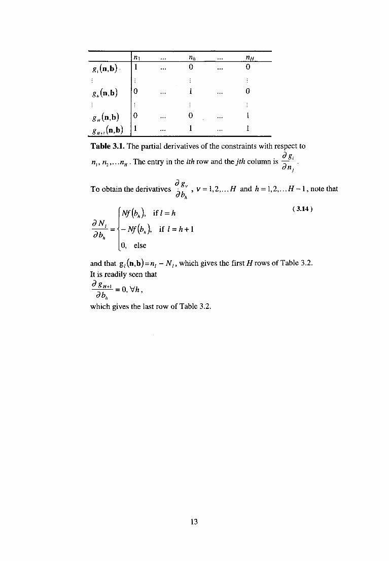
Table 3.1. The partial derivatives of the constraints with respect to

nt,n2,...nH. The entry in the ith row and the jth column is ——.

dg To obtain the derivatives -r—^, v = 1,2,... H and h = l,2,...H-I, note that

dbh

( 3.14 )

and that g, (n,b) -nt - Nt, which gives the first H rows of Table 3.2. It is readily seen that

o 8H+\ n W ; — — = 0, Vh,

dbh

which gives the last row of Table 3.2.

13

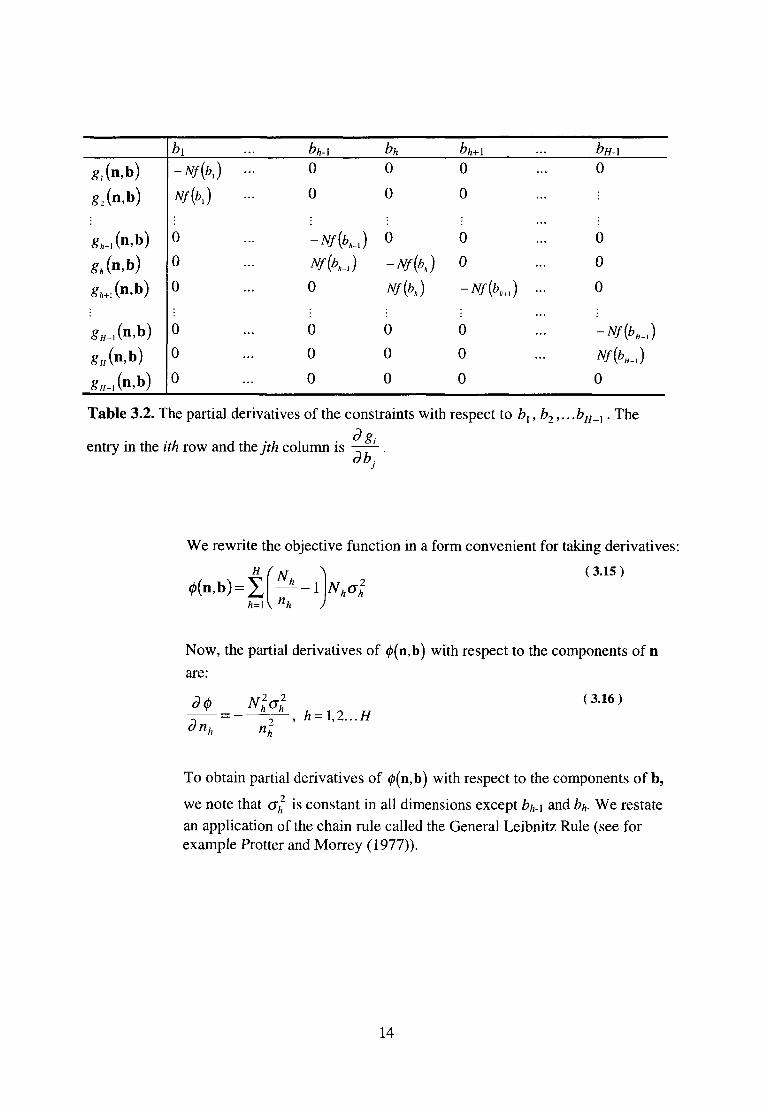
Table 3.2. The partial derivatives of the constraints with respect to b1,b2,.. -bH_1. The

entry in the ith row and the jth column is -r—L . db;

We rewrite the objective function in a form convenient for taking derivatives:

( 3.15 )

Now, the partial derivatives of 0(n,b) with respect to the components of n are:

( 3.16 )

To obtain partial derivatives of 0(n,b) with respect to the components of b,

we note that <7A2 is constant in all dimensions except bh-\ and bh- We restate

an application of the chain rule called the General Leibnitz Rule (see for example Protter and Morrey (1977)).

14

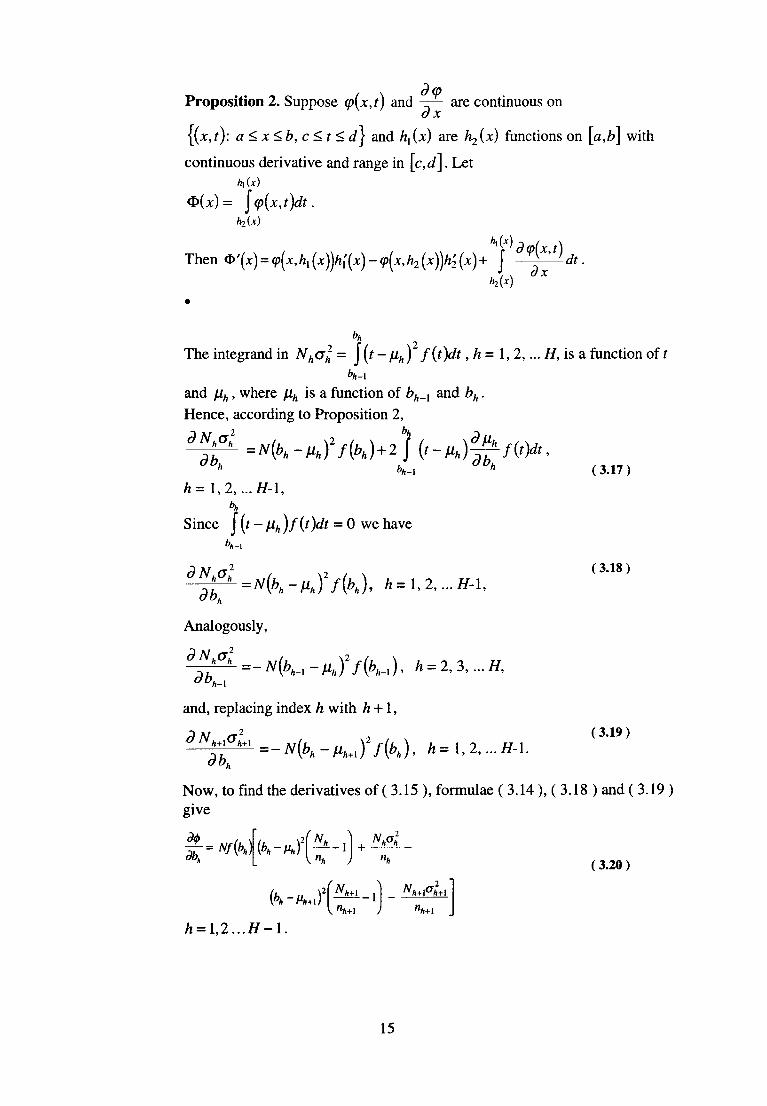
Proposition 2. Suppose <p\x,t) and -r— are continuous on ox

continuous derivative and range in [c,d]. Let

The integrand in . H, is a function of t

and fih, where \Lh is a function of bh_{ and &A. Hence, according to Proposition 2,

(3.17)

Since

( 3.18 )

Analogously,

and, replacing index h with h +1,

(3.19)

Now, to find the derivatives of ( 3.15 ), formulae ( 3.14 ), ( 3.18 ) and ( 3.19 ) give

(3.20)

15

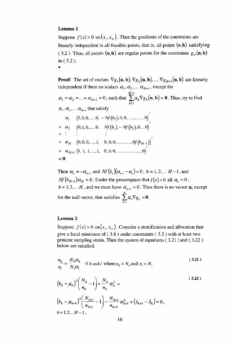
Lemma 1

Suppose f(x) > 0 on (xt ,xN). Then the gradients of the constraints are

linearly independent in all feasible points, that is, all points (n,b) satisfying

( 3.2 ). Thus, all points (n,b) are regular points for the constraints gv (n,b)

in ( 3.2 ). •

Proof: The set of vectors Vg1 (n, b), Vg2 (n, b), . . . Vg#+1 (n, b) are linearly

independent if there no scalars CC1,GC2,... ccH+l, except for H+l

a\ =a2 =•••= ccH+l - 0, such that ^ ^ h ^ S h ( n , b) = 0. Thus, try to find

ax, a2,... aH+i that satisfy

Nf {bH_x )aH = 0. Under the presumption that f(x) > 0 all cch = 0,

h = 1,2,... H, and we must have aH+l - 0. Thus there is no vector a, except H

for the null vector, that satisfies ^cchVgh =0.

Lemma 2

Suppose f(x) > 0 on^ , ,xN ) . Consider a stratification and allocation that

give a local minimum of ( 3.8 ) under constraints ( 3.2 ) with at least two genuine sampling strata. Then the system of equations ( 3.21 ) and ( 3.22 ) below are satisfied.

( 3.21 )

( 3.22 )

16

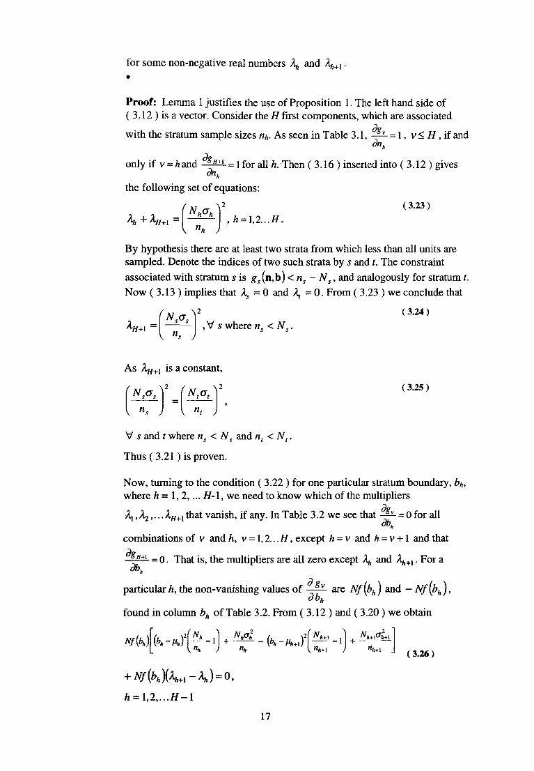
for some non-negative real numbers \ and Xh+l. •

Proof: Lemma 1 justifies the use of Proposition 1. The left hand side of ( 3.12 ) is a vector. Consider the H first components, which are associated

de with the stratum sample sizes nh. As seen in Table 3.1, -^- = 1, v< H, if and

dnh de

only if v = Aand -£z±i- = lfor all h. Then ( 3.16 ) inserted into ( 3.12 ) gives dnh

the following set of equations:

( 3.23 )

By hypothesis there are at least two strata from which less than all units are sampled. Denote the indices of two such strata by s and t. The constraint associated with stratum s is ^ ( i^b) <ns - Ns, and analogously for stratum t. Now (3.13) implies that Xs = 0 and X, = 0. From ( 3.23 ) we conclude that

(3.24)

As XH+l is a constant,

( 3.25 )

Thus (3.21 ) is proven.

Now, turning to the condition ( 3.22 ) for one particular stratum boundary, bh, where h = 1, 2,... H-1, we need to know which of the multipliers

\ , ^2,... XH+l that vanish, if any. In Table 3.2 we see that -^- = 0 for all dbh

combinations of v and h, v = 1,2... H, except h = v and h = v +1 and that H+l = 0. That is, the multipliers are all zero except Xh and Xh+l. For a

dbh

particular A, the non-vanishing values of ~^- are Nf(bh) and - Nf[bh),

found in column bh of Table 3.2. From (3.12) and ( 3.20 ) we obtain

( 3.26 )

17

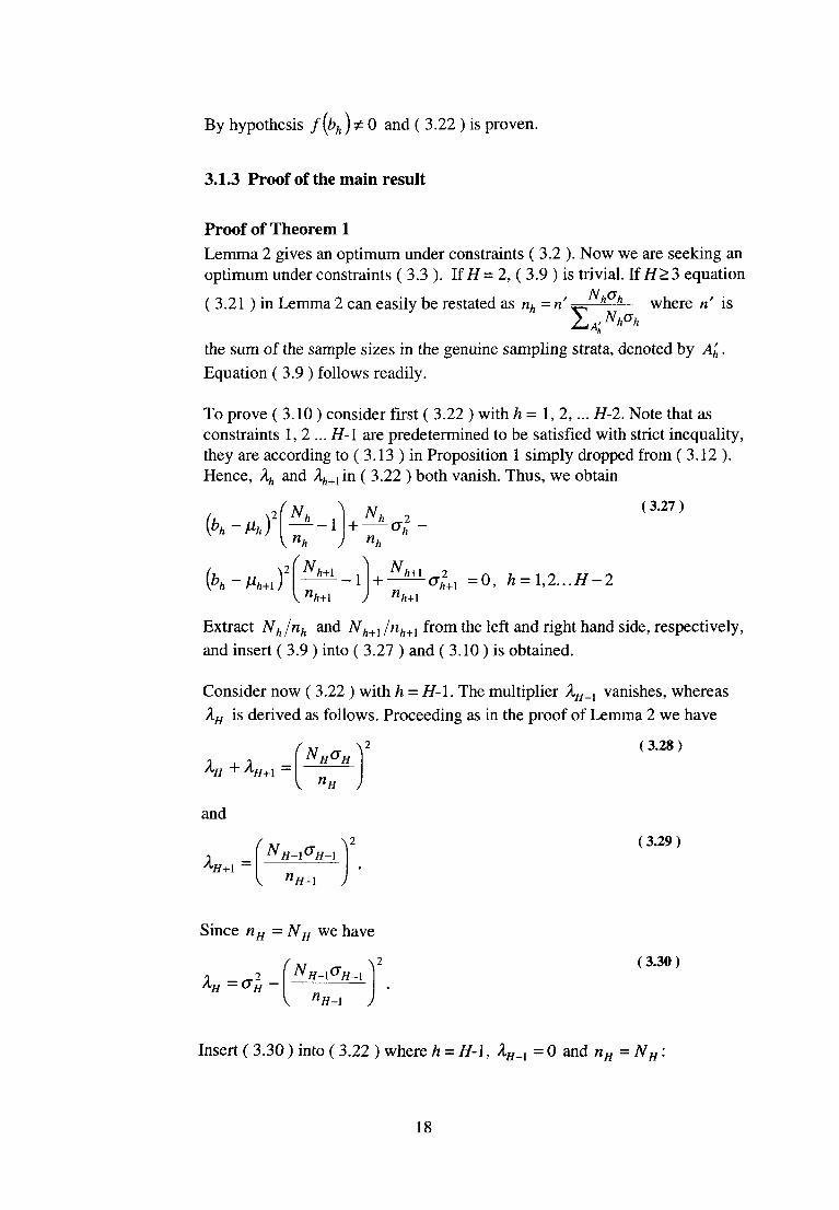
By hypothesis f(bh)ïO and ( 3.22 ) is proven.

3.1.3 Proof of the main result

Proof of Theorem 1 Lemma 2 gives an optimum under constraints ( 3.2 ). Now we are seeking an optimum under constraints ( 3.3 ). If H = 2, ( 3.9 ) is trivial. If H> 3 equation

(3.21 ) in Lemma 2 can easily be restated as nh = n' h h— where n is

the sum of the sample sizes in the genuine sampling strata, denoted by A'h.

Equation ( 3.9 ) follows readily.

To prove ( 3.10 ) consider first ( 3.22 ) with h = 1, 2,... H-2. Note that as constraints 1, 2 ... H-\ are predetermined to be satisfied with strict inequality, they are according to ( 3.13 ) in Proposition 1 simply dropped from ( 3.12 ). Hence, Xh and Aft+1in ( 3.22 ) both vanish. Thus, we obtain

(3.27)

Extract Nh/nh and Nh+l /nh+l from the left and right hand side, respectively, and insert ( 3.9 ) into ( 3.27 ) and ( 3.10 ) is obtained.

Consider now ( 3.22 ) with h = H-\. The multiplier XH_{ vanishes, whereas XH is derived as follows. Proceeding as in the proof of Lemma 2 we have

( 3.28 )

and

( 3.29 )

Since nH = Af# we have

( 3.30 )

18

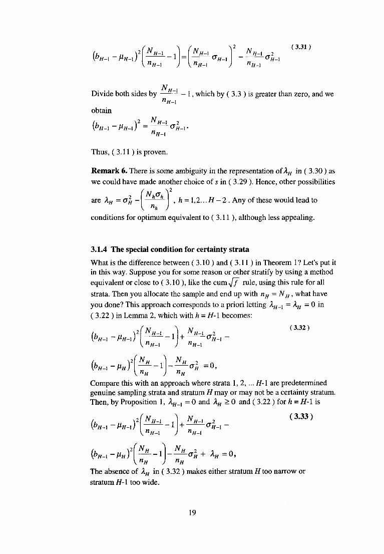
( 3.31 )

Divide both sides by 1, which by ( 3.3 ) is greater than zero, and we

obtain

Thus, ( 3.11 ) is proven.

Remark 6. There is some ambiguity in the representation of XH in ( 3.30 ) as we could have made another choice of s in ( 3.29 ). Hence, other possibilities

. Any of these would lead to

conditions for optimum equivalent to ( 3.11 ), although less appealing.

3.1.4 The special condition for certainty strata

What is the difference between (3.10) and ( 3.11 ) in Theorem 1 ? Let's put it in this way. Suppose you for some reason or other stratify by using a method equivalent or close to ( 3.10 ), like the cum-//7 rule, using this rule for all strata. Then you allocate the sample and end up with nH = NH, what have you done? This approach corresponds to a priori letting XE_X = XH = 0 in ( 3.22 ) in Lemma 2, which with h = H-l becomes:

( 3.32 )

Compare this with an approach where strata 1, 2,... H-\ are predetermined genuine sampling strata and stratum H may or may not be a certainty stratum. Then, by Proposition 1, lH_x = 0 and XH > 0 and ( 3.22 ) for h = H-\ is

( 3.33 )

The absence of XH in ( 3.32 ) makes either stratum H too narrow or stratum H-\ too wide.

19

Lavallée, Hidiroglou (1988) applied the Dalenius-Hodges rule and their own method (see section 2) to two highly skewed populations. The Dalenius-Hodges rule resulted in a much narrower certainty stratum for both populations, for all coefficients of variations requirements and for all choices of parameter/) in power allocation. Their intention by using the Dalenius-Hodges rule to determine the size of a certainty stratum, despite the fact that the Dalenius-Hodges rule is derived under Approximation 1, is to "caution against its blind use in the context of highly skewed populations" (Lavallée, Hidiroglou (1988, p. 40)).

20

4 A Numerical Procedure for Stratification

In this section a numerical procedure for the optimum stratification problem is presented. The situation we have in mind is as follows.

There is a frame where all units have values for an auxiliary variable

x = |x, , x2,... xN }. The distribution of the values of x is assumed highly

skewed, which calls for a certainty stratum containing the largest units. All other strata are genuine sampling strata. The strata, denoted by Ay, A2,... AH, are to be determined by stratum boundary points that yield a solution to the optimum stratification problem under constraints ( 3.3 ). The solution is given by conditions ( 3.10 ) and ( 3.11 ) in Theorem 1. Once the strata are determined, the sample is allocated to strata according to condition ( 3.9 ) in Theorem 1.

However, we shall be satisfied with an approximate solution to ( 3.10 ). In doing so, we rely on the experience that the estimator variance is flat around the optimal stratum boundaries bx, b2,.. .bH_2 for genuine sampling strata. This is further discussed in section 5.

Against this background we use Approximation 1 for genuine sampling strata which simplifies (3.10) to the Dalenius equations ( 2.4 ). As already mentioned, a number of easy-to-use approximate methods have been proposed to solve ( 2.4 ). We shall be concerned with the one proposed by Ekman (1959). The degree of approximation to an exact solution of ( 2.4 ) is discussed by Ekman. References of some empirical studies are given in section 2 "Overview of the optimum stratification problem". As Ekman notes, his rule is "substantially equivalent" to the widely used Dalenius-Hodges rule (Ekman, 1959, pp 223-224).

4.1 The stratification algorithm

We aim at boundaries for genuine sampling strata given by a solution to the Dalenius equations ( 2.4 ) and at a boundary for the certainty stratum given by condition ( 3.11 ) in Theorem 1. The set of equations ( 2.4 ) requires a numerical method to be solved. Below we state the extended Ekman rule and propose an algorithm for it. Moreover, we propose an algorithm for the combined problem of using the extended Ekman rule for the genuine sampling strata and the condition ( 3.11 ) for the certainty stratum. This algorithm is now described.

The stratification algorithm The algorithm will go through possible values of the size of the certainty stratum, from NH = 0 to NH = n, and for each value the other stratum boundaries are determined by the extended Ekman rule.

21

1. Let NH = 0.

2. Stratify the frame with stratum H removed into H-\ strata with the extended Ekman rule. Apply the numerical procedure for stratification by the extended Ekman rule shown below.

3. Calculate the left and right hand side, respectively, of equation (3.11 ) in Theorem 1. Save the values in a file.

4. Transfer the K units with the largest x-values from stratum H-1 to stratum H (where K is a small positive integer, for example, K - 1).

5. Repeat steps 2-4 until NH = n.

6. Plot the values from step 3 against NH . You will see two curves which cross at 0, 1, 2... points. If they cross once, a solution to ( 3.11 ) is found, that is, the optimal size of the certainty stratum is found. The boundaries given by step 2 are approximately optimal sizes of the genuine sampling strata. If the curves do not cross, there is no solution with a certainty stratum. In this case, stratify the frame with the extended Ekman rule into H strata. If the curves cross at more than one point, all the points have to be evaluated. This plot will be referred to as the certainty stratum plot (an example is shown in Figure 5.4).

Clearly, this algorithm will produce all points that satisfy equation ( 3.11 ) in Theorem 1 and the extended Ekman rule.

4.2 A numerical procedure for stratification by the extended Ekman rule

When discussing the Ekman rule and its extended version (below) we assume that the size of the certainty stratum, NH , is known. In subsection 4.2 we consider the remainder of the frame after removal of the certainty stratum. Let this part be sorted by the stratification variable. Denote the minimum value by x\ and maximum one by xN_N .

Let #E denote the number of elements in a set E.

The Ekman stratification rule: Let Nh = #Ah, where Ah is stratum h, h = 1, 2, ... H-l. Set b0 = xx and

Determine the stratum boundary points bx, b2,...bH_2 so as to satisfy the following relation as well as possible.

(4.1)

Remark. The reason for the slightly vague term "as well as possible" is that (4.1) usually lacks an exact solution whenN1,N2,...NH_} are confined to

22

integers. The extended Ekman rule, given below, admits non-integral Nl,N2,--.Nfj^ and produces an exact solution under general conditions.

4.2.1 A geometric interpretation of the Ekman rule

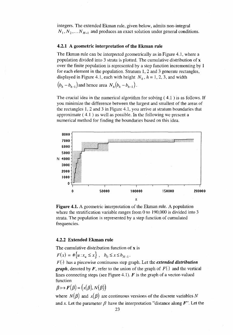
The Ekman rule can be interpreted geometrically as in Figure 4.1, where a population divided into 3 strata is plotted. The cumulative distribution of x over the finite population is represented by a step function incrementing by 1 for each element in the population. Stratum 1, 2 and 3 generate rectangles, displayed in Figure 4.1, each with height Nh,h= 1, 2, 3, and width

and hence area Nh (bh - bh_x ) .

The crucial idea in the numerical algorithm for solving (4.1 ) is as follows. If you minimize the difference between the largest and smallest of the areas of the rectangles 1, 2 and 3 in Figure 4.1, you arrive at stratum boundaries that approximate ( 4.1 ) as well as possible. In the following we present a numerical method for finding the boundaries based on this idea.

Figure 4.1. A geometric interpretation of the Ekman rule. A population where the stratification variable ranges from 0 to 190,000 is divided into 3 strata. The population is represented by a step function of cumulated frequencies.

4.2.2 Extended Ekman rule

The cumulative distribution function of x is

F(-) has a piecewise continuous step graph. Let the extended distribution graph, denoted by F, refer to the union of the graph of F(-) and the vertical lines connecting steps (see Figure 4.1). F is the graph of a vector-valued function

where N[p) and x(/3j are continuous versions of the discrete variables N

and x. Let the parameter /? have the interpretation "distance along F". Let the 23

minimum and maximum values of /? be P0=0 and

By an extended stratum boundary point we mean any point on the graph F. We will denote the H-2 extended stratum boundary points we are interested in by fi{, fi2,... flH_2. Given a [3h, the corresponding proper stratum

boundary bh is the horizontal position x( fih J of F. There is a natural order of

the extended stratum boundary points and the endpoints, let them satisfy P0 < (31 < fi2 <•••< PH-I • I n t n e extended situation we allow formation of

rectangles with lower left and upper right corner anywhere along F, including the vertical parts of it. We refer to the them as Ekman rectangles. The area of Ekman rectangle h is

The counterpart to ( 4.1 ) becomes

(4.2)

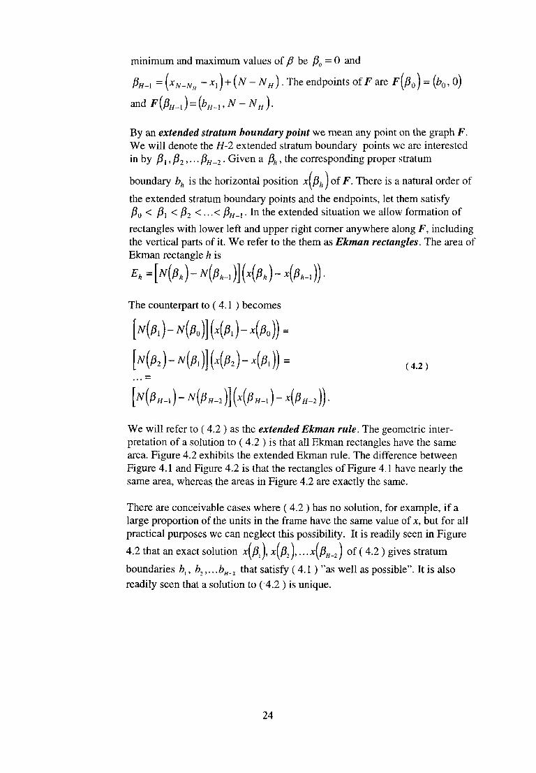
We will refer to ( 4.2 ) as the extended Ekman rule. The geometric inter­pretation of a solution to ( 4.2 ) is that all Ekman rectangles have the same area. Figure 4.2 exhibits the extended Ekman rule. The difference between Figure 4.1 and Figure 4.2 is that the rectangles of Figure 4.1 have nearly the same area, whereas the areas in Figure 4.2 are exactly the same.

There are conceivable cases where ( 4.2 ) has no solution, for example, if a large proportion of the units in the frame have the same value of x, but for all practical purposes we can neglect this possibility. It is readily seen in Figure

4.2 that an exact solution x(ftl ), xW2 ),...xiPH_2) of ( 4.2 ) gives stratum

boundaries bi, b2,.. .bH_2 that satisfy ( 4.1 ) "as well as possible". It is also readily seen that a solution to ( 4.2 ) is unique.

24

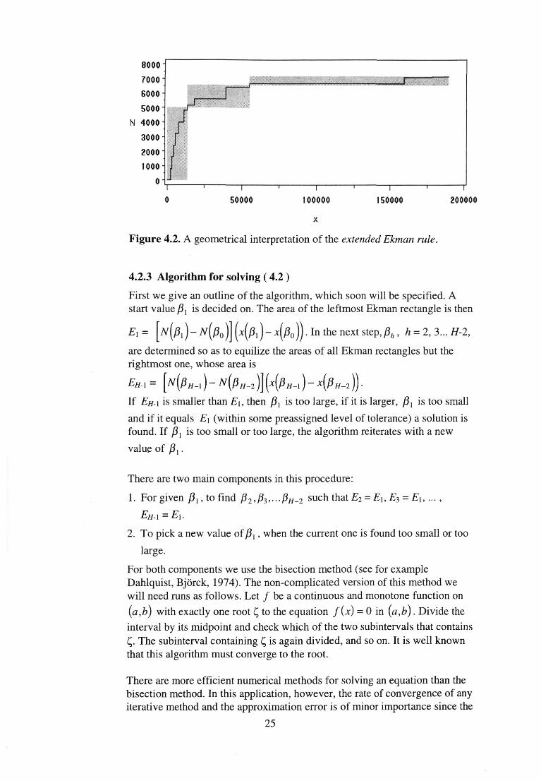
Figure 4.2. A geometrical interpretation of the extended Ekman rule.

4.2.3 Algorithm for solving ( 4.2 )

First we give an outline of the algorithm, which soon will be specified. A start value (3i is decided on. The area of the leftmost Ekman rectangle is then

In the next step,

are determined so as to equilize the areas of all Ekman rectangles but the rightmost one, whose area is

If EH-\ is smaller than E\, then fix is too large, if it is larger, {5X is too small

and if it equals E\ (within some preassigned level of tolerance) a solution is found. If y3j is too small or too large, the algorithm reiterates with a new

value of /J,.

There are two main components in this procedure:

1. Forgiven J5X, to find /?2,/?3,...j3//-2 s u c n that £2 = E\,E$ = E\,...,

EH-I = E\.

2. To pick a new value of /?,, when the current one is found too small or too

large.

For both components we use the bisection method (see for example Dahlquist, Björck, 1974). The non-complicated version of this method we will need runs as follows. Let / be a continuous and monotone function on

(a,b) with exactly one root Ç to the equation f(x) = 0 in (a,b). Divide the interval by its midpoint and check which of the two subintervals that contains Ç The subinterval containing Ç is again divided, and so on. It is well known that this algorithm must converge to the root.

There are more efficient numerical methods for solving an equation than the bisection method. In this application, however, the rate of convergence of any iterative method and the approximation error is of minor importance since the

25

application is basically of discrete nature. There is no point in pursuing the algorithm until j3, can be determined with a good number of significant

decimals. Therefore, the comparatively simple bisection method is proposed.

Next, two of the steps of the algorithm that solves ( 4.2 ) are described separately.

Computation of extended stratum boundary points

Let /?!, and thus Eu be given. In order to find the area of the second rectangle

with an area E% that equals E\, one wants to find the value of j82 that solves

the equation

(4.3)

The function

is continuous and strictly decreasing on \BÏ, PH_y J. Therefore, Zij32) has at

most one root in W{, /?#_, J. There is exactly one root if Zm, J > 0 and

z(pH_l ) < 0. There is no root if z(/3, ) > 0 and z(pH_x ) > 0. In this case p2

and E2 are set to missing.

The algorithm above is formulated for j82, given fix. It is repeated for the

pairs (j82, j83), (/?3,04),. . . [pH_3, PH-2 ) • If A is missing in a pair

f j8, ,Pj), then /3 and £} are set to missing.

Classification of extended stratum boundary points

A tolerance Ô > 0 is specified. After all extended stratum boundary points A , P2, •.. PH_2 are computed, the point /?, is classified. If the rightmost

Ekman rectangle, EH-U is non-missing it is either smaller than, larger than or equal to (with tolerance 8) E\. If it is missing, it is considered smaller than E\. We classify fi{ into the three possible outcomes:

This classification divides the graph F into three parts according to the value of /?j : the first part where /?, is too small, the second one where it is good

and the last part where /?, is too large.

26

An algorithm that solves ( 4.2 )

1. Specify a pair ( flx , /?, J of a too small and a too large value of /Jj, for

example (Po,pH-i)-

2. Compute the arithmetic mean . Denote it fix .

3. Compute (32, ...PH^2 given /3X = j8, and classify Px into good, too small

or too large.

4. If / ^ is good, a solution of ( 4.2 ) is found and the algorithm is

terminated.

Else if j8, is too small, go to step 1 and replace ( j3, , (5{ 1 with

Else if /J, is too large, go to step 1 and replace (/?, , fix I with I /3j , /?, j .

27

5 Applications

In this section we give some numerical illustrations of the results in section 3 and 4. We worked under the assumption that the study variable is equal to the stratification variable. There are at least two reasons for studying practical applications under this assumption: - Theorem 1 was derived under the assumption that the discrete distribution

x can sufficiently well be approximated by a continuous distribution. This suggests that there may exist a stratification with lower variance than a stratification that satisfies the conditions of Theorem 1. It is therefore of interest to see how Theorem 1 works in practice (compare Remark 5 in section 3).

- It is interesting to compare the results of this report to those of other authors who work under the same assumption.

The two populations introduced next were considered.

5.1 The value added population

The annual census of Swedish manufacturing industry collects data on sales, cost of materials, energy used in the production process, etc. The value added is derived. The census together with derived variables is frequently used as a sampling frame for other surveys. We used the 1989 frame with value added as stratification variable. This frame, which in the sequel is referred to as the value added population, contains 7326 establishments. Its skewness is 12.4 (which could be compared with skewness 2.0 of an exponential distribution).

5.2 The log-normal population

An artificial population was created by 2000 random numbers generated from a log-normal distribution X = ez where Z is univariate normal with mean 4 and variance 2.7 (further details in Appendix A). Again it is a highly skewed population, the skewness being 26.7.

5.3 General framework for the simulations

In the simulations we divided given populations into H = 4 strata. The stratum comprising units with the largest values of the stratification variable was a certainty stratum, the other strata were genuine sampling strata. A sample size was determined. The sample was allocated according to Theorem 1, that is, with stratum H as a certainty stratum, the allocation rule is

(5.1)

where 5/, is the standard deviation of the stratification variable within stratum h. We will call this x-optimal allocation (thus adhering to the terminology of Särndal, Swensson, Wretman, 1992).

28

5.4 Performance measure

5.4.1 Best possible stratification

Due to the approximation mentioned in the first paragraph of section 5 there may exist a stratification with lower variance than a stratification that satisfies the conditions of Theorem 1. For each situation considered in this section we searched for the stratification with the least estimator variance (3.1 ), which we refer to as the best possible stratification.

The values xx, x2,.. .xN of the stratification variable furnish the set of all potential stratum boundaries. A boundary bh anywhere in the interval \xk_x ,xk), where £-1 and k are two adjacent units in the ordered population, give the same estimator variance as the boundary bh = xk_}, provided the other boundaries remain unchanged. If bh = xk_{, unit k-\ belongs to stratum h. In the considered situations, with H = 4 strata, a stratification is specified by the boundaries bx,b2 and b3. Alternatively, since the population size Nis given, a stratification is specified by three of the stratum sizes NX,N2, N3 and NA. Clearly, as we now consider a specific situation, with specified values of x = xl,x2,...xN, sample size n and number of strata H, there exists a best possible stratification (a global minimum). We denote the estimator variance by Var(t; N), where N = (N], N2, N3 ).

For both populations studied, Var(t; Nf) was computed for a large number of

combinations of N,, N2 and N3. Under variation of the three stratification

parameters the estimator variance forms a response surface in a four-

dimensional space. Let pj be the response surface projected on the two-

dimensional space (Nj, Var(t; N)| for j = 1, 2, 3 and 4. Figure 5.1 shows a

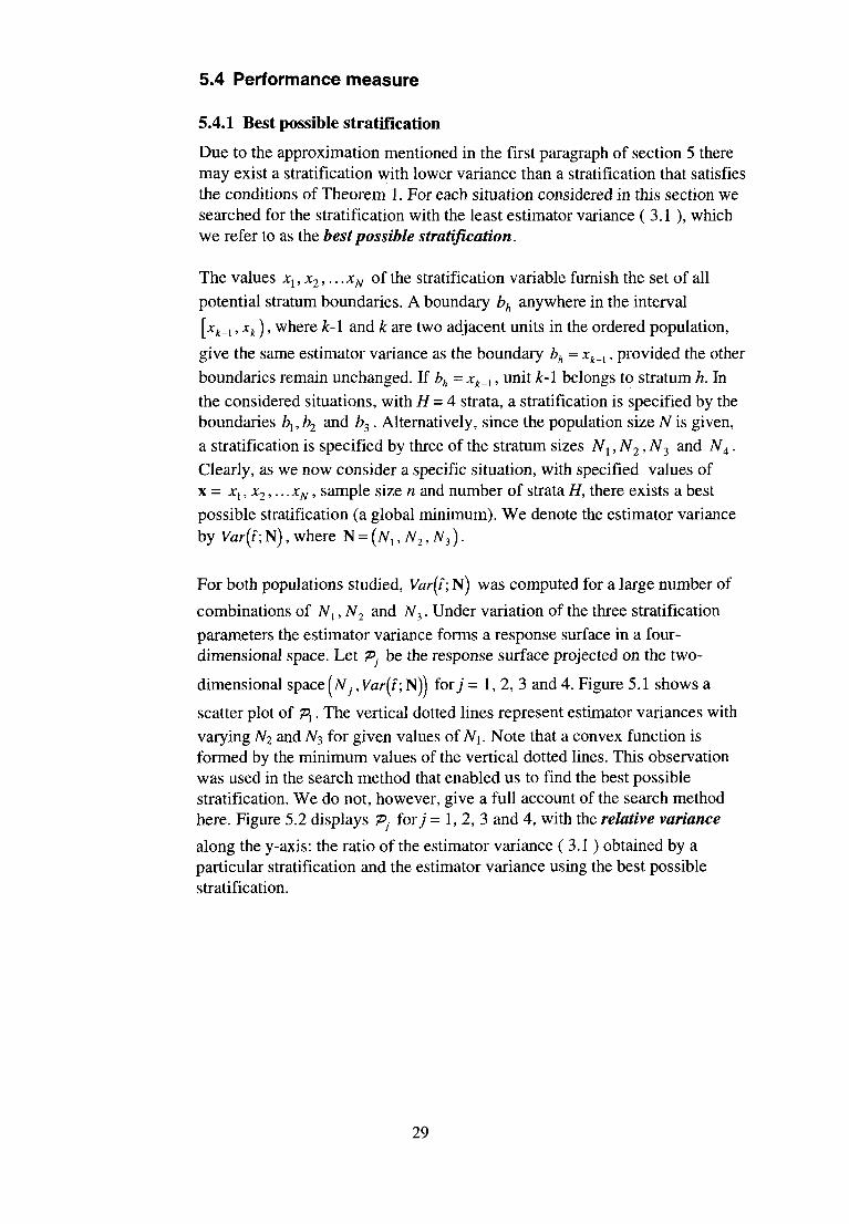
scatter plot of Px. The vertical dotted lines represent estimator variances with varying N2 and N3 for given values of N^. Note that a convex function is formed by the minimum values of the vertical dotted lines. This observation was used in the search method that enabled us to find the best possible stratification. We do not, however, give a full account of the search method here. Figure 5.2 displays Pj for; = 1, 2, 3 and 4, with the relative variance

along the y-axis: the ratio of the estimator variance ( 3.1 ) obtained by a particular stratification and the estimator variance using the best possible stratification.

29

Size of stratum 1

Figure 5.1. The estimator variance surface for a large number of stratifications of the log-normal population, projected on the plane given by N1 and the variance (divided by 109).

Size of sfratum 1

Size of sfratum 2

30

Size of stratum 3

Size of stratum 4

Figure 5.2. The relative variance of a large number of stratifications of the log-normal population. In scatter plot (a) different sizes of stratum 1, N\, are plotted along the x-axis. The vertical dotted lines represent relative variances with varying N2 and N3 given a value of N\. Scatter plots (b), (c) and (d) display exactly the same stratifications as (a), although with N2, N3 and N4, respectively, along the x-axis.

5.4.2 Best possible stratification of the value added population

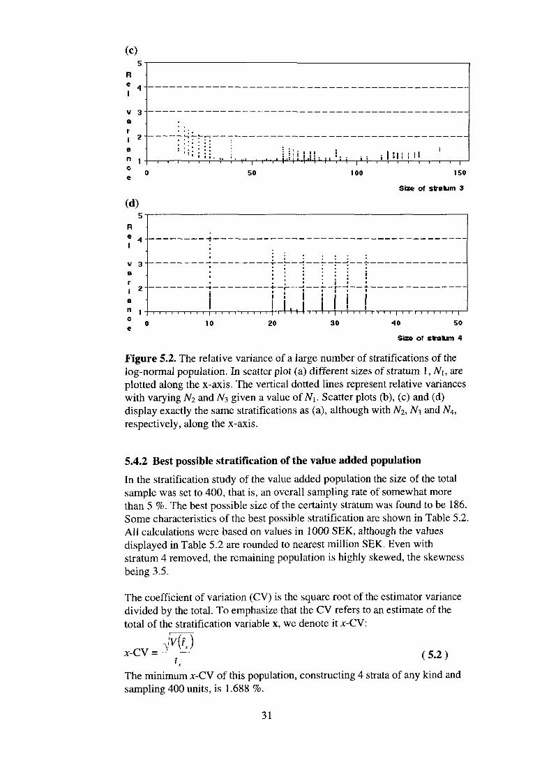
In the stratification study of the value added population the size of the total sample was set to 400, that is, an overall sampling rate of somewhat more than 5 %. The best possible size of the certainty stratum was found to be 186. Some characteristics of the best possible stratification are shown in Table 5.2. All calculations were based on values in 1000 SEK, although the values displayed in Table 5.2 are rounded to nearest million SEK. Even with stratum 4 removed, the remaining population is highly skewed, the skewness being 3.5.

The coefficient of variation (CV) is the square root of the estimator variance divided by the total. To emphasize that the CV refers to an estimate of the total of the stratification variable x, we denote it x-CV:

(5.2)

The minimum x-CV of this population, constructing 4 strata of any kind and sampling 400 units, is 1.688 %.

31

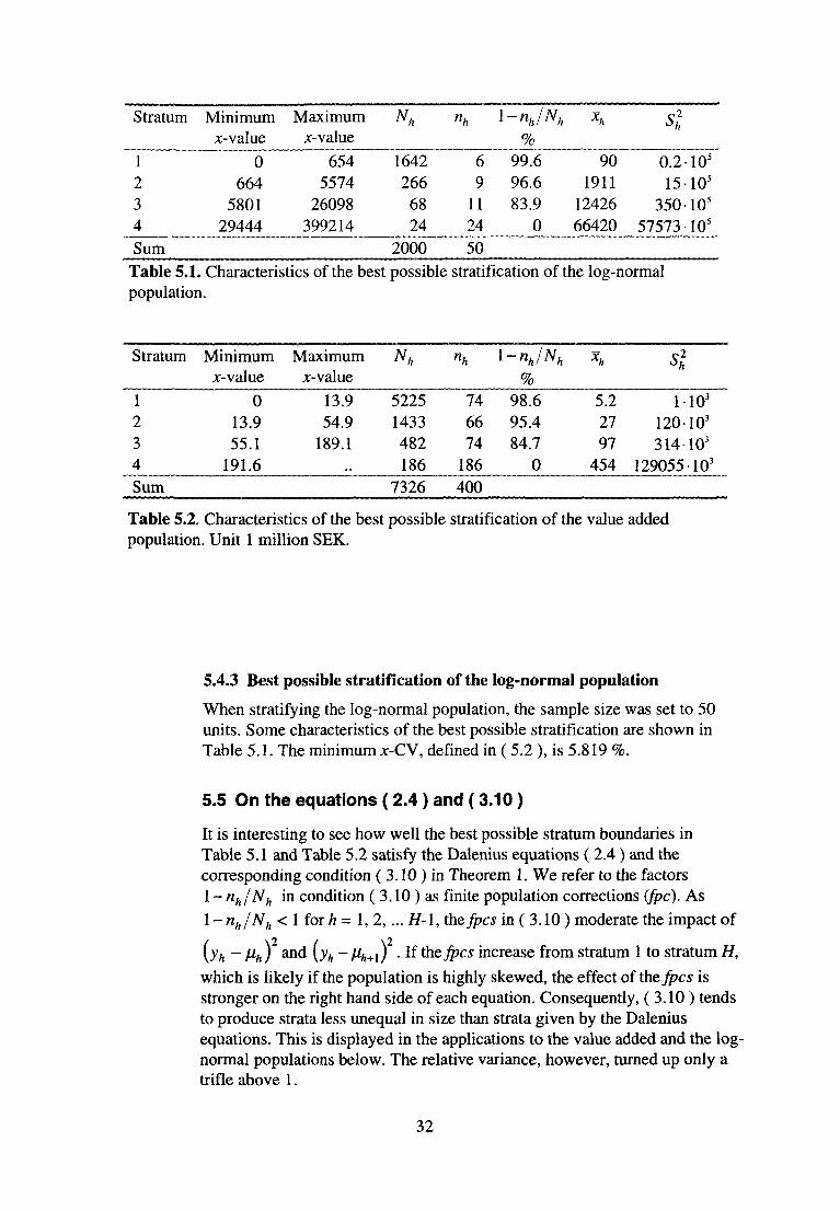
Table 5.1. Characteristics of the best possible stratification of the log-normal population.

Table 5.2. Characteristics of the best possible stratification of the value added population. Unit 1 million SEK.

5.4.3 Best possible stratification of the log-normal population

When stratifying the log-normal population, the sample size was set to 50 units. Some characteristics of the best possible stratification are shown in Table 5.1. The minimum x-CV, defined in ( 5.2 ), is 5.819 %.

5.5 On the equations ( 2.4 ) and ( 3.10 )

It is interesting to see how well the best possible stratum boundaries in Table 5.1 and Table 5.2 satisfy the Dalenius equations ( 2.4 ) and the corresponding condition ( 3.10 ) in Theorem 1. We refer to the factors l-nh/Nh in condition ( 3.10 ) as finite population corrections ifpc). As \-nh/Nh < 1 for/i= 1, 2,... H-l, theses in ( 3.10 ) moderate the impact of

[yh - \ih ) and \yh - fih+l) . If theses increase from stratum 1 to stratum H,

which is likely if the population is highly skewed, the effect of the Jpcs is stronger on the right hand side of each equation. Consequently, ( 3.10 ) tends to produce strata less unequal in size than strata given by the Dalenius equations. This is displayed in the applications to the value added and the log-normal populations below. The relative variance, however, turned up only a trifle above 1.

32

5.5.1 Equations ( 2.4 ) and ( 3.10 ) applied to the value added population

The characteristics of the best possible stratification for the genuine sampling strata (strata 1, 2 and 3 given in Table 5.2) were inserted in the Dalenius equations ( 2.4 ) and in system ( 3.10 ) in Theorem 1. A value of the right and

Figure 5.3. The best possible stratum boundaries for the value added population (from Table 5.2) inserted into ( 2.4 ) and into ( 3.10 ). The bars represent the value (in thousands) of the left and right hand side, respectively, of (2.4) and (3.10).

left hand side, respectively, were obtained for each of the equations with h = 1,2. Figure 5.3 exhibits those values. Notice a discrepancy between the left and the right hand side for the Dalenius equation associated with stratum 2, whereas the best possible boundaries satisfy ( 3.10 ) almost exactly for both stratum 1 and 2.

It is also interesting to analyse the problem the other way around. The stratification in Table 5.3 is a solution to the Dalenius equations in the following sense. Usually, when ( 2.4 ) is applied to a finite population an exact solution does not exist. The stratum boundaries b\ and b2 shown in Table 5.3 minimize D] + D2 where

The boundaries b\ and b2 are the maximum x-values within strata. Stratum 4 is fixed to 186 units which is its best possible size. The relative variance turned out to be 1.004, that is, only slightly above 1.

33

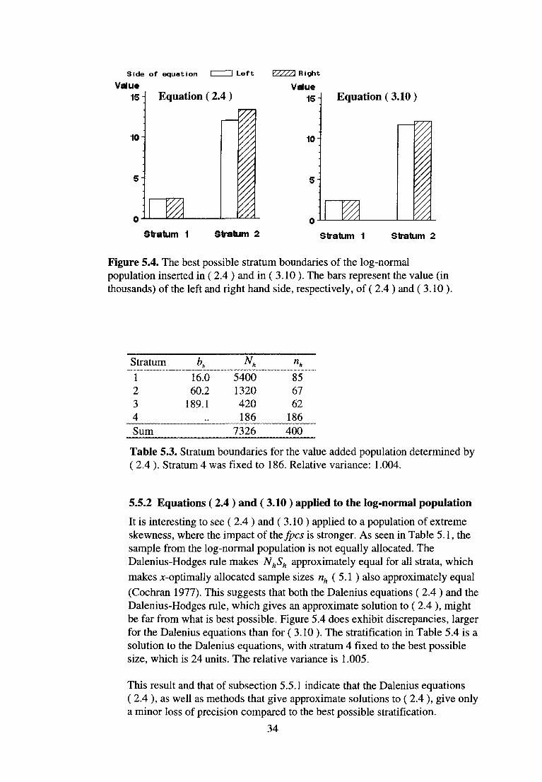
Figure 5.4. The best possible stratum boundaries of the log-normal population inserted in ( 2.4 ) and in ( 3.10 ). The bars represent the value (in thousands) of the left and right hand side, respectively, of ( 2.4 ) and ( 3.10 ).

Table 5.3. Stratum boundaries for the value added population determined by ( 2.4 ). Stratum 4 was fixed to 186. Relative variance: 1.004.

5.5.2 Equations ( 2.4 ) and ( 3.10 ) applied to the log-normal population

It is interesting to see ( 2.4 ) and ( 3.10 ) applied to a population of extreme skewness, where the impact of theses is stronger. As seen in Table 5.1, the sample from the log-normal population is not equally allocated. The Dalenius-Hodges rule makes NhSh approximately equal for all strata, which makes x-optimally allocated sample sizes nh (5.1 ) also approximately equal (Cochran 1977). This suggests that both the Dalenius equations ( 2.4 ) and the Dalenius-Hodges rule, which gives an approximate solution to ( 2.4 ), might be far from what is best possible. Figure 5.4 does exhibit discrepancies, larger for the Dalenius equations than for ( 3.10 ). The stratification in Table 5.4 is a solution to the Dalenius equations, with stratum 4 fixed to the best possible size, which is 24 units. The relative variance is 1.005.

This result and that of subsection 5.5.1 indicate that the Dalenius equations ( 2.4 ), as well as methods that give approximate solutions to ( 2.4 ), give only a minor loss of precision compared to the best possible stratification.

34

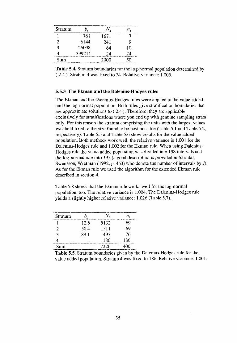
Table 5.4. Stratum boundaries for the log-normal population determined by ( 2.4 ). Stratum 4 was fixed to 24. Relative variance: 1.005.

5.5.3 The Ekman and the Dalenius-Hodges rules

The Ekman and the Dalenius-Hodges rules were applied to the value added and the log-normal population. Both rules give stratification boundaries that are approximate solutions to ( 2.4 ). Therefore, they are applicable exclusively for stratifications where you end up with genuine sampling strata only. For this reason the stratum comprising the units with the largest values was held fixed to the size found to be best possible (Table 5.1 and Table 5.2, respectively). Table 5.5 and Table 5.6 show results for the value added population. Both methods work well, the relative variance is 1.001 for the Dalenius-Hodges rule and 1.002 for the Ekman rule. When using Dalenius-Hodges rule the value added population was divided into 198 intervals and the log-normal one into 195 (a good description is provided in Sarndal, Swensson, Wretman (1992, p. 463) who denote the number of intervals by J). As for the Ekman rule we used the algorithm for the extended Ekman rule described in section 4.

Table 5.8 shows that the Ekman rule works well for the log-normal population, too. The relative variance is 1.004. The Dalenius-Hodges rule yields a slightly higher relative variance: 1.026 (Table 5.7).

Table 5.5. Stratum boundaries given by the Dalenius-Hodges rule for the value added population. Stratum 4 was fixed to 186. Relative variance: 1.001.

35

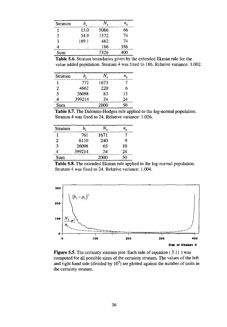
Table 5.6. Stratum boundaries given by the extended Ekman rule for the value added population. Stratum 4 was fixed to 186. Relative variance: 1.002.

Table 5.7. The Dalenius-Hodges rule applied to the log-normal population. Stratum 4 was fixed to 24. Relative variance: 1.026.

Table 5.8. The extended Ekman rule applied to the log-normal population. Stratum 4 was fixed to 24. Relative variance: 1.004.

Figure 5.5. The certainty stratum plot. Each side of equation (3.11 ) was computed for all possible sizes of the certainty stratum. The values of the left and right hand side (divided by 109) are plotted against the number of units in the certainty stratum.

36

5.6 The stratification algorithm

5.6.1 The stratification algorithm applied to the value added population

Using the stratification algorithm (section 4) the value added population was divided into 4 strata. The extended Ekman rule was used to construct stratum 1, 2 and 3, while condition ( 3.11 ) in Theorem 1 provided the boundary of stratum 4. We used the stratification algorithm with K = 1. The plot described in step 6 of the stratification algorithm is shown in Figure 5.5. The curves cross at N4 = 186, which coincides with the best possible size of stratum 4 (see Table 5.2). Hence, the extended Ekman rule applied to the value added population minus stratum 4 with N4 = 186 yields the stratification displayed in Table 5.6. Thus the relative variance given by the stratification algorithm is 1.002.

5.6.2 The stratification algorithm applied to the log-normal population

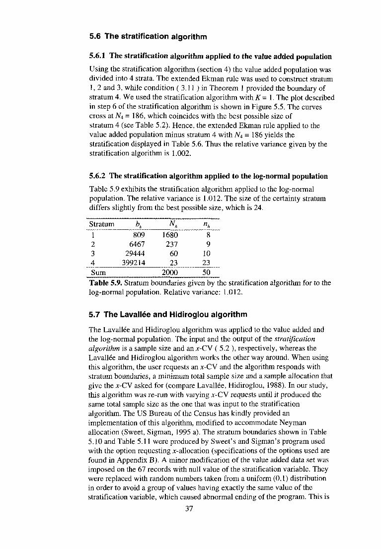
Table 5.9 exhibits the stratification algorithm applied to the log-normal population. The relative variance is 1.012. The size of the certainty stratum differs slightly from the best possible size, which is 24.

Table 5.9. Stratum boundaries given by the stratification algorithm for to the log-normal population. Relative variance: 1.012.

5.7 The Lavallée and Hidiroglou algorithm

The Lavallée and Hidiroglou algorithm was applied to the value added and the log-normal population. The input and the output of the stratification algorithm is a sample size and an x-CV ( 5.2 ), respectively, whereas the Lavallée and Hidiroglou algorithm works the other way around. When using this algorithm, the user requests an x-CW and the algorithm responds with stratum boundaries, a minimum total sample size and a sample allocation that give the x-CV asked for (compare Lavallée, Hidiroglou, 1988). In our study, this algorithm was re-run with varying JC-CV requests until it produced the same total sample size as the one that was input to the stratification algorithm. The US Bureau of the Census has kindly provided an implementation of this algorithm, modified to accommodate Neyman allocation (Sweet, Sigman, 1995 a). The stratum boundaries shown in Table 5.10 and Table 5.11 were produced by Sweet's and Sigman's program used with the option requesting x-allocation (specifications of the options used are found in Appendix B). A minor modification of the value added data set was imposed on the 67 records with null value of the stratification variable. They were replaced with random numbers taken from a uniform (0,1) distribution in order to avoid a group of values having exactly the same value of the stratification variable, which caused abnormal ending of the program. This is

37

discussed in Sweet and Sigman (1995 a, p 10). As seen in Table 5.10 and Table 5.11 the strata and the relative variances are similar to those obtained with the stratification algorithm (see Table 5.6 and Table 5.9).

Table 5.10. Stratum boundaries given by the Lavallée and Hidiroglou method for the value added population. Relative variance: 1.001.

Table 5.11. Stratum boundaries given by the Lavallée and Hidiroglou method for the log-normal population. Relative variance: 1.018.

5.8 Flatness of the Objective Function

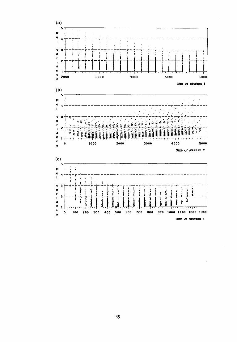
The JC-CV and the relative variance were computed for 2856 stratifications of the value added population. In Figure 5.6 (a), (b), (c) and (d) the relative variance is plotted against the size of each stratum (it is the same type of figure as Figure 5.2). Recall that this population contains 7326 units and that the sample size was set to 400. The most striking feature of the plots in Figure 5.6 is the flatness of the estimator variance surface. Plot (d), for

example, shows that if the size of the certainty stratum is within (l20,230) it

is possible to hit the minimum variance if the other strata are chosen

optimally. The interval (120, 230) must be considered very wide as the

certainty stratum with a total sample size of 400 cannot contain more than 400 units. If the certainty stratum is chosen within this interval and the three genuine sampling strata are determined by the Ekman rule, the worst relative variance is 1.05 (achieved for N4 = 120). This repeated for the interval

(140, 230) gives 1.02 as the worst relative variance (achieved for N4 = 230).

A large certainty stratum combined with a small size of stratum 3 yields relative variances that are unacceptable.

The log-normal population shows similar flatness (Figure 5.2).

38

39

(a)

(b)

(c)

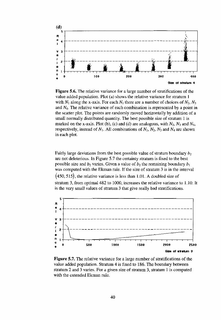
Figure 5.6. The relative variance for a large number of stratifications of the value added population. Plot (a) shows the relative variance for stratum 1 with N\ along the x-axis. For each N\ there are a number of choices of N2, N3 and N4. The relative variance of each combination is represented by a point in the scatter plot. The points are randomly moved horizontally by addition of a small normally distributed quantity. The best possible size of stratum 1 is marked on the x-axis. Plot (b), (c) and (d) are analogous, with N2, N3 and N4, respectively, instead of M. All combinations of N\, N2, N3 and N4 are shown in each plot.

Fairly large deviations from the best possible value of stratum boundary b2

are not deleterious. In Figure 5.7 the certainty stratum is fixed to the best possible size and b2 varies. Given a value of b2 the remaining boundary b\ was computed with the Ekman rule. If the size of stratum 3 is in the interval

(450,515) , the relative variance is less than 1.01. A doubled size of

stratum 3, from optimal 482 to 1000, increases the relative variance to 1.10. It is the very small values of stratum 3 that give really bad stratifications.

Figure 5.7. The relative variance for a large number of stratifications of the value added population. Stratum 4 is fixed to 186. The boundary between stratum 2 and 3 varies. For a given size of stratum 3, stratum 1 is computed with the extended Ekman rule.

40

As a concluding remark, suppose a frame is divided into H strata where the stratum containing the largest units, stratum H, is a certainty stratum and all other strata are genuine sampling strata and suppose the number of units in the frame is substantially greater than H. Then, in most practical applications, the estimator variance surface is flat around the best possible stratum boundaries. Hence, a moderate deviation from the best possible values of bx, b2,.. .bH_2 should increase the variance only negligibly. The variance around bH_x is fairly flat, although not necessarily as flat as around the other stratum boundaries.

To the knowledge of the author, there is no support of the intuitive feeling that the variance is flat around the optimal boundaries of genuine sampling strata, other than empirical data. For example Dalenius and Gurney (1951, p 141) say as a final remark supporting Approximation 1 in the optimum stratification problem:

...as is often the case with optimum solutions in sampling, slight deviations from the absolute optimum value have almost no practical importance.

Acknowledgement: The author wishes to express his gratitude to colleagues at Statistics Sweden, in particular Professor Bengt Rosén, for encouragement and constructive criticism.

41

References

Cochran, W.G. (1977). Sampling Techniques, 3rd éd., New York: Wiley.

Cochran, W.G. (1961). Comparison of Methods for Determining Stratum Boundaries. Bulletin de l'Institut International de Statistique, Vol. 38:2, pp. 345-357.

Dahlquist, G., Björck, Å. (1974). Numerical Methods. Prentice-Hall.

Dalenius, T. (1950), The Problem of Optimum Stratification. Skandinavisk Aktuarietidskrift, pp. 203-213

Dalenius, T.; Gurney, M. (1951). The Problem of Optimum Stratification. II. Skandinavisk Aktuarietidskrift, pp. 133-148.

Dalenius, T. (1952). The Problem of Optimum Stratification in a Special Type of Design. Skandinavisk Aktuarietidskrift, pp. 61-70.

Dalenius, T.; Hodges, J.L. (1959). Minimum Variance Stratification. Journal of the American Statistical Association, Vol. 54, pp. 88-101.

Detlefsen, R. E.; Veum, S. C. (1991). Design Issues for the Retail Trade Sample Surveys of the U.S. Bureau of the Census. Proceedings of the Survey Research Methods. American Statistical Association, pp. 214-219.

Ekman, G. (1959). An Approximation Useful in Univariate Stratification. The Annals of Mathematical Statistics, Vol. 30:1, pp. 219-229.

Glasser, G.J. (1962). On the Complete Coverage of Large Units in a Statistical Study. Review of the International Statistical Institute, Vol. 30:1, pp. 28-32.

Hess, I., Sethi, V.K. and Balakrishnan, T.R. (1966). Stratification: A Practical Investigation. Journal of the American Statistical Association, Vol. 61, pp. 74-90.

Hidiroglou, M. A. (1986). The Construction of a Self-Representing Stratum of Large Units in Survey Design. The American Statistician, Vol. 40:1, pp. 27-31.

Hidiroglou, M. A., Srinath K. P. (1993). Problems Associated with Designing Subannual Business Surveys. Journal of Business & Economic Statistics, Vol. 11, No. 4, pp. 397-405.

Lavâllée P.; Hidiroglou, M. A. (1988). On the stratification of Skewed Populations. Survey Methodology, Vol. 14, No. 1, pp. 33-43.

Luenberger, D. G. (1973). Introduction to linear and nonlinear programming. Reading, Massachusetts: Addison-Wesley.

Murthy, M.N. (1967). Sampling Theory and Methods. Statistical Publishing Society, Calcutta.

Protter, M. H.; Morrey, C. B. (1977). A First Course in Real Analysis. New York: Springer-Verlag.

Särndal, C.-E.; Swensson, B.; Wretman J. (1992). Model Assisted Survey Sampling. New York: Springer-Verlag.

Schneeberger, H. (1985). Maxima, Minima und Sattelpunkte bei optimaler Schichtung und optimaler Aufteilung. Allgemeines Statistisches Archiv, Vol. 69:3, pp. 286-297.

42

Sigman, R.; Monsour, N. (1995). Selecting Samples from List Frames of Business. In: B. Cox, D. Binder, N. Chinappa, A. Christianson, M. Colledge, P. Kött (eds.J, Business Survey Methods. New York: Wiley, pp. 133-152.

Slanta, J.; Krenzke, T. (1996). Applying the Lavallée and Hidiroglou Method to Obtain Stratification Boundaries for the Census Bureau's Annual Capital Expenditures Survey. Survey Methodology, Vol. 22, No. 1, pp. 65-75.

Sweet, E. M. and Sigman R. S. (1995 a). User Guide for the Generalized SAS Univariate Stratification Program. ESM Report Series, ESM-9504. Bureau of the Census.

Sweet, E. M.; Sigman R. S. (1995 b). Evaluation of Model-Assisted Procedures for stratifying skewed populations using auxiliary data. Proceedings of the Survey Research Methods, Vol I. American Statistical Association, pp. 491 -496.

43

Appendix A

The SAS-program below created the log-normal population used in the simulation studies. The program was run on SAS version 6.12 under Windows 95.

45

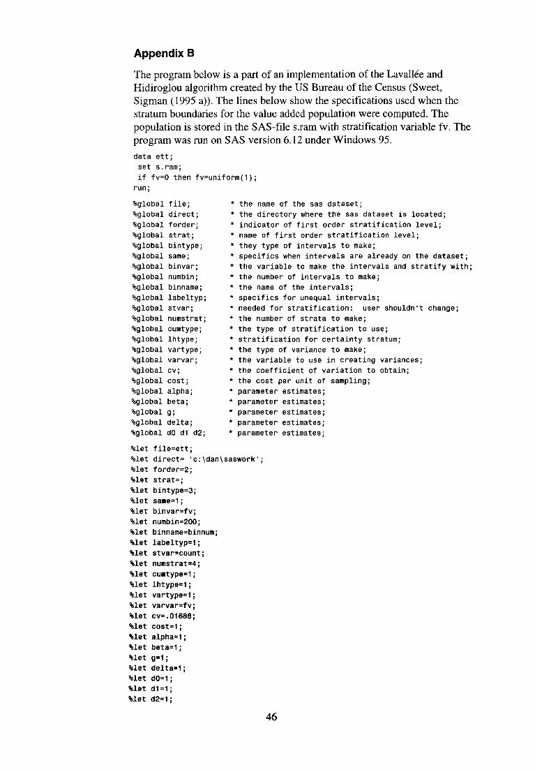
Appendix B

The program below is a part of an implementation of the Lavallée and Hidiroglou algorithm created by the US Bureau of the Census (Sweet, Sigman (1995 a)). The lines below show the specifications used when the stratum boundaries for the value added population were computed. The population is stored in the SAS-file s.ram with stratification variable fv. The program was run on SAS version 6.12 under Windows 95.

46