R/Bioconductor course Predictive Networks: a new · PDF fileR/Bioconductor course Predictive Networks: a new framework for ... Harvard School of ... Erik Bakke, James Hardwick, Gianluca

R/Bioconductor coursePredictive Networks: a new framework for inferring robust

networks from gene expression data

Benjamin Haibe-Kains1,2

1Computational Biology and Functional Genomics Laboratory, Dana-Farber CancerInstitute, Harvard School of Public Health

2Center for Cancer Computational Biology, Dana-Farber Cancer Institute

May 24, 2011

Contents

1 Introduction 3

2 Biology and Data 42.1 RAS signaling pathway . . . . . . . . . . . . . . . . . . . . . . . . . . . . . . . . 42.2 Colon cancer gene expression data . . . . . . . . . . . . . . . . . . . . . . . . . . 42.3 Known gene interactions extracted from the biomedical literature and public struc-

tured databases . . . . . . . . . . . . . . . . . . . . . . . . . . . . . . . . . . . . 52.4 Predictionet package . . . . . . . . . . . . . . . . . . . . . . . . . . . . . . . . . 5

3 Network inference from priors and gene expression data 73.1 Methodology . . . . . . . . . . . . . . . . . . . . . . . . . . . . . . . . . . . . . . 73.2 Network inference with predictionet . . . . . . . . . . . . . . . . . . . . . . . . . . 93.3 Edge-specific stability . . . . . . . . . . . . . . . . . . . . . . . . . . . . . . . . . 153.4 Gene-specific prediction score . . . . . . . . . . . . . . . . . . . . . . . . . . . . . 163.5 Predictionet and Cytoscape . . . . . . . . . . . . . . . . . . . . . . . . . . . . . . 20

4 Comparison of network inference with respect to the priors 244.1 Comparison of edge-specific prediction scores . . . . . . . . . . . . . . . . . . . . 254.2 Comparison of gene-specific prediction score . . . . . . . . . . . . . . . . . . . . . 27

5 Comparison of network inference with respect to the training data 30

6 Future works 35

1

Disclaimer

This work was supervised by John Quackenbush and it has been done in collaboration with Catha-rina Olsen, Christopher Bouton, Erik Bakke, James Hardwick, Gianluca Bontempi, Amira Djebbari,Niall Prendergast, and Renee Rubio.

Materials

All the materials required for this course are incorporated in the predictionet package which isavailable from https://github.com/bhaibeka/predictionet.

2

https://github.com/bhaibeka/predictionet

1 Introduction

DNA microarrays and other high-throughput omics technologies provide large datasets that ofteninclude patterns of correlation between genes reflecting the complex processes that underlie cellularprocesses. The challenge in analyzing large-scale expression data has been to extract biologicallymeaningful inferences regarding these processes – often represented as networks – in an environ-ment where the datasets are complex and noisy. Although many techniques have been developedin an attempt to address these issues, to date their ability to extract meaningful and predictivenetwork relationships has been limited.

In this course, I will introduce a platform developed in John Quackenbush’s lab, which enablesinference of reliable gene interaction networks from prior biological knowledge, in the form ofbiomedical literature and structured databases, and from gene expression data. Using real data, Iwill show the benefit of using prior biological knowledge to infer networks and how to quantitativelyassess the quality of such networks.

Tutorial This tutorial describes in detail all the necessary steps to infer a gene interaction networkcombining prior biological knowledge and gene expression data.

Our approach is the following:

1. Select a gene expression dataset and a list of genes of interest.

2. Extract priors from the biomedical literature and public structured databases using thePredictive Networks web application.

3. Use the predictionet R package to infer a gene interaction network from priors and geneexpression data.

(a) Infer a network using the main function netinf.

(b) Explore and display the topology of the resulting network.

(c) Assess the stability of the network inference in cross-validation (function netinf.cv).

(d) Assess quantitatively the predictive ability of the network in cross-validation (functionnetinf.cv).

(e) Assess quantitatively the predictive ability of the network in a fully independent dataset(functions netinf.predict and pred.score).

4. Use predictionet to statistically compare multiple gene interaction networks.

Using two colon cancer gene expression datasets as examples (see Section 2) we go step bystep and provide all the R code necessary to perform the entire analysis.

3

2 Biology and Data

For this tutorial, we focus on colon cancer and more specifically the RAS signaling pathway.

2.1 RAS signaling pathway

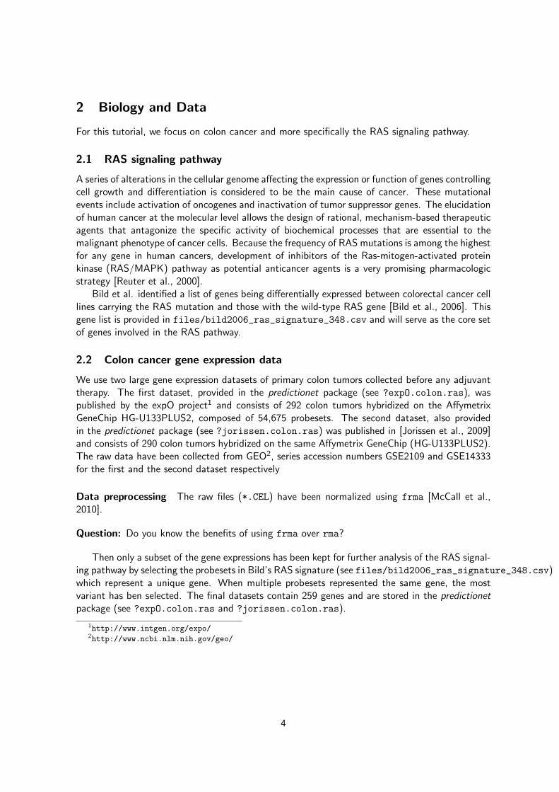
A series of alterations in the cellular genome affecting the expression or function of genes controllingcell growth and differentiation is considered to be the main cause of cancer. These mutationalevents include activation of oncogenes and inactivation of tumor suppressor genes. The elucidationof human cancer at the molecular level allows the design of rational, mechanism-based therapeuticagents that antagonize the specific activity of biochemical processes that are essential to themalignant phenotype of cancer cells. Because the frequency of RAS mutations is among the highestfor any gene in human cancers, development of inhibitors of the Ras-mitogen-activated proteinkinase (RAS/MAPK) pathway as potential anticancer agents is a very promising pharmacologicstrategy [Reuter et al., 2000].

Bild et al. identified a list of genes being differentially expressed between colorectal cancer celllines carrying the RAS mutation and those with the wild-type RAS gene [Bild et al., 2006]. Thisgene list is provided in files/bild2006_ras_signature_348.csv and will serve as the core setof genes involved in the RAS pathway.

2.2 Colon cancer gene expression data

We use two large gene expression datasets of primary colon tumors collected before any adjuvanttherapy. The first dataset, provided in the predictionet package (see ?expO.colon.ras), waspublished by the expO project1 and consists of 292 colon tumors hybridized on the AffymetrixGeneChip HG-U133PLUS2, composed of 54,675 probesets. The second dataset, also providedin the predictionet package (see ?jorissen.colon.ras) was published in [Jorissen et al., 2009]and consists of 290 colon tumors hybridized on the same Affymetrix GeneChip (HG-U133PLUS2).The raw data have been collected from GEO2, series accession numbers GSE2109 and GSE14333for the first and the second dataset respectively

Data preprocessing The raw files (*.CEL) have been normalized using frma [McCall et al.,2010].

Question: Do you know the benefits of using frma over rma?

Then only a subset of the gene expressions has been kept for further analysis of the RAS signal-ing pathway by selecting the probesets in Bild’s RAS signature (see files/bild2006_ras_signature_348.csv)which represent a unique gene. When multiple probesets represented the same gene, the mostvariant has ben selected. The final datasets contain 259 genes and are stored in the predictionetpackage (see ?expO.colon.ras and ?jorissen.colon.ras).

1http://www.intgen.org/expo/2http://www.ncbi.nlm.nih.gov/geo/

4

http://www.intgen.org/expo/

http://www.ncbi.nlm.nih.gov/geo/

2.3 Known gene interactions extracted from the biomedical literature and publicstructured databases

In order to extract previously published gene interactions, Prof John Quackenbush initiated thedevelopment of the Predictive Networks web application [https://compbio.dfci.harvard.edu/predictivenetworks/] implemented by Dr Christopher Bouton and his team at Entagen3.This tool enables users to easily retrieve a large number of high quality gene interactions reportedin the biomedical literature (full-text open-access PubMed articles and/or MEDLINE abstracts)and/or structured biological databases (e.g., Pathway Commons) by focussing on a core set ofgenes (referred to as gene list).

One can use the Predictive Networks web application to retrieve a list of interactions involvingat least one gene included in our list of RAS-related genes. To do so, one has to first create anaccount to login to the webapp. Then go to ”My Page”and create a new gene list by cutting-and-pasting the gene symbols4 included in files/bild2006_ras_signature_348.csv. Lastly, wehave to export all the resulting triples (e.g., ”genea regulates geneb represented by the interactiongenea → geneb”) in a CSV file by clicking on ”View Triples” and then ”Download w/ SentencesAs”. One can use R to read this file and count how many times a gene interaction has beenobserved in the biomedical literature and reported structured biological databases. Actually theresults of such manipulations have been incorporated into the predictionet package as describedbelow.

2.4 Predictionet package

Let’s install the predictionet package using the following command

> install.packages(pkgs = "predictionet_0.9.tar.gz", repos = NULL)

If some dependencies are missing, such as the igraph, catnet, and penalized packages, youcan install them using the install.packages and specify the Comprehensive R Archive Network(CRAN) as repository

> install.packages("penalized", repos = "http://cran.r-project.org",

+ dependencies = TRUE)

If the package has to be installed on a Windows machine, the compilation may fail becauseyou lack of a proper C compiler. Then we should use the R GUI and install the file predic-

tionet_0.9.zip that was precompiled specifically for Windows.

Let’s load the predictionet package:

> library(predictionet)

We are now able to run all the functions implemented in the predictionet package. These functionsare listed in the documentation of the package itself.

3http://www.entagen.com4Be extremely careful if you use Microsoft Excel since it will automatically interpret SEPT6, that is gene ”SEPTIN

6”, as the 6th of September!

5

https://compbio.dfci.harvard.edu/predictivenetworks/

https://compbio.dfci.harvard.edu/predictivenetworks/

> library(help = predictionet)

Looking at the help page of expO.colon.ras and jorissen.colon.ras will give the detailsabout the data that we will use during this course.

> help(expO.colon.ras)

> help(jorissen.colon.ras)

expO.colon.ras and jorissen.colon.ras contain three R objects:

data*.ras matrix of gene expression data; tumors in rows, probes in columns.

annot*.ras data frame of probe annotations; probes in rows, annotations in columns.

demo*.ras data frame of clinical information of the colon cancer patients; patients in rows,clinical variables in columns.

priors*.ras matrix of prior information about the gene interactions; parents/sources in rows,children:targets in columns.

Although the objects data*.ras, and demo*.ras are specific to each dataset, the objectsdata*.ras and data*.ras are common in the two datasets under study because the samemicroarray technology has been used to generate them and we extracted the same genes, andsubsequently the same known gene interactions (priors).

Question: By looking at the dimensions of these objects, can you deduce for how many geneswe have the gene expression data?

Question: How many interactions between those genes have been reported in the literature andbiological structured databases? Hint: look at the priros.ras object.

6

3 Network inference from priors and gene expression data

Many methods have been developed for network inference: Bayesian networks, nested q-partialgraphs, information-theoretic networks, regression-based networks,. . . These methods differ greatlyin their way of dealing with the potentially high dimensionality of the problem, handling missingvalues, learning from observations and/or interventions, combining genomic data and prior knowl-edge, assessing the quality of fitted networks, and their ability to make predictions.

In this course, I present a regression-based network inference approach we specifically developed

• to deal efficiently with large number of genes (potentially ≥ 100),

• to avoid discretization of the input values,

• to combine prior knowledge and gene expression data,

• to infer stable gene interaction networks,

• to make predictions about the expression of genes of interest in independent data.

3.1 Methodology

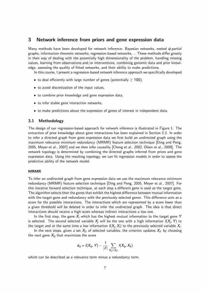
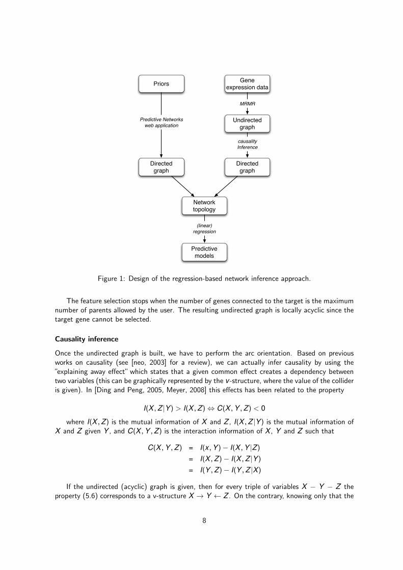
The design of our regression-based approach for network inference is illustrated in Figure 1. Theextraction of prior knowledge about gene interactions has been explained in Section 2.3. In orderto infer a directed graph from gene expression data we first build an undirected graph using themaximum relevance minimum redundancy (MRMR) feature selection technique [Ding and Peng,2005, Meyer et al., 2007] and we then infer causality [Cheng et al., 2002, Olsen et al., 2009]. Thenetwork topology is determined by combining the directed graphs inferred from priors and geneexpression data. Using the resulting topology, we can fit regression models in order to assess thepredictive ability of the network model.

MRMR

To infer an undirected graph from gene expression data we use the maximum relevance minimumredundancy (MRMR) feature selection technique [Ding and Peng, 2005, Meyer et al., 2007]. Forthis iterative forward selection technique, at each step a different gene is used as the target gene.The algorithm selects then the genes that exhibit the highest difference between mutual informationwith the target gene and redundancy with the previously selected genes. This difference acts as ascore for the possible interactions. The interactions which are represented by a score lower thana given threshold will be deleted in order to infer the undirected graph. The idea is that directinteractions should receive a high score whereas indirect interactions a low one.

In the first step, the gene Xi which has the highest mutual information to the target gene Yis selected. The second selected variable Xj will be the one with a high information I(Xj , Y ) tothe target and at the same time a low information I(Xj , Xi ) to the previously selected variable Xi .

In the next steps, given a set XS of selected variables, the criterion updates XS by choosingthe next gene Xq that maximizes the score

sq = I(Xq, Y )− 1|S|

∑Xk∈XS

I(Xq, Xk )

which can be described as a relevance term minus a redundancy term.

7

Gene expression data

Undirected graph

Directedgraph

Directedgraph

Networktopology

Predictive models

Priors

MRMR

causalityInference

(linear)regression

Predictive Networksweb application

Figure 1: Design of the regression-based network inference approach.

The feature selection stops when the number of genes connected to the target is the maximumnumber of parents allowed by the user. The resulting undirected graph is locally acyclic since thetarget gene cannot be selected.

Causality inference

Once the undirected graph is built, we have to perform the arc orientation. Based on previousworks on causality (see [neo, 2003] for a review), we can actually infer causality by using the”explaining away effect” which states that a given common effect creates a dependency betweentwo variables (this can be graphically represented by the v -structure, where the value of the collideris given). In [Ding and Peng, 2005, Meyer, 2008] this effects has been related to the property

I(X , Z |Y ) > I(X , Z )⇔ C(X , Y , Z ) < 0

where I(X , Z ) is the mutual information of X and Z , I(X , Z |Y ) is the mutual information ofX and Z given Y , and C(X , Y , Z ) is the interaction information of X , Y and Z such that

C(X , Y , Z ) = I(x , Y )− I(X , Y |Z )= I(X , Z )− I(X , Z |Y )= I(Y , Z )− I(Y , Z |X )

If the undirected (acyclic) graph is given, then for every triple of variables X − Y − Z theproperty (5.6) corresponds to a v-structure X → Y ← Z . On the contrary, knowing only that the

8

interaction information is less than zero does not help with inferring the network because the threepossible differences between mutual information and conditional mutual are equivalent. Thus, itis not evident which variable should be the collider.

Therefore, the only possibility for orienting the arcs using the interaction information is to usethe following property:

Given three variables X , Y and Z and a structure X − Y − Z , then if I(X , Z |Y ) >I(X , Z ), i.e., C(X , Y , Z ) < 0, then X → Y ← Z

Depending on the data, we can now identify some of the genes as parents.

Combination with priors

To infer the final network topology, we combine, for each interaction between genei and genej ,the score based on priors (Pij) and MRMR+causality inference (Mij). We let users control theweight put on the priors, i.e., their confidence on the prior knowledge gathered on internet:

wPij + (1− w)Mij

where w ∈ [0, 1].Users can then easily infer networks using prior knowledge only (w = 1) or using gene expression

data only (w = 0). However, we will see in our real case study that a combination of priors andgene expression data usually yields inference of better networks.

Predictive ability of the network model

The last step of our network inference approach is the fitting of local regression models to enableprediction of gene expressions. To do so, we fit a linear regression model for each gene in networksusing its parents as predictors.

This novel approach is implemented in the predictionet package and is also integrated in thePredictive Networks web application (see ”Analysis”panel). Even if the package is not yet availablefrom BioConductor5, a public Git repository is accessible from https://github.com/bhaibeka/

predictionet; any non-violent and constructive feedback is welcome. ,

3.2 Network inference with predictionet

Let’s infer our first network and go through the main options of the package. The main functionof the predictionet package is netinf with the following key parameters: .

data Matrix of continuous or categorical values with observations in rows and features in columns.

categories If this parameter missing, data should be already discretized; otherwise either a singleinteger or a vector of integers specifying the number of categories used to discretize eachvariable (data are then discretized using equal-frequency bins) or a list of cutoffs to use todiscretize each of the variables in data matrix. If method=’bayesnet’ and categories ismissing, data should contain categorical values and the number of categories will determinefrom the data.

5http://www.bioconductor.org

9



http://www.bioconductor.org

perturbations Matrix of {0, 1} specifying whether a gene has been perturbed (e.g., knockdown,over-expression) in some experiments. Dimensions should be the same than data.

priors Matrix of prior information available for gene-gene interaction (parents in rows, children incolumns). Values may be probabilities or any other weights (citations count for instance). ifpriors counts are used the parameter priors.ras should be TRUE so the priors are scaledaccordingly.

predn Indices or names of variables to fit during network inference. If missing, all the variables willbe used for network inference. Note that for bayesian network inference (method=’bayesnet’)this parameter is ignored and a network will be generated using all the variables.

priors.ras TRUE if priors specified by the user are number of citations (count) for each interaction,FALSE if probabilities or any other weight in [0,1] are reported instead.

priors.weight Real value in [0,1] specifying the weight to put on the priors (0=only the data areused, 1=only the priors are used to infer the topology of the network).

maxparents Maximum number of parents allowed for each gene.

subset Vector of indices to select only subset of the observations.

method ’bayesnet’ for Bayesian network inference with the catnet package (not implementedyet), ’regrnet’ for regression-based network inference.

causal TRUE if the causality should be inferred from the data, FALSE otherwise

seed Set the seed to make the network inference deterministic.

You can easily access this description by consulting the help page of the netinf

> help(netinf)

The netinf function returns a list containing the names of the method used for networkinference, the network topology and a list of local regression models.You can infer a gene interaction network using the expO dataset data.ras, by equally balancingthe importance of priors and data in the network inference process (priors.weight = 0.5).

To reduce the computational time, we will focus on the top 35 genes which are the mostdifferentially expressed between RAS mutated and wild type cell lines:

> ## number of genes to select for the analysis

> genen <- 35

> ## select only the top genes

> goi <- dimnames(annot.ras)[[1]][order(abs(log2(annot.ras[,

"fold.change"])),

+ decreasing = TRUE)[1:genen]]

Now run the network inference on the reduced expO.colon.ras dataset:

> mynet <- netinf(data = data.ras[, goi], priors = priors.ras[goi,

10

+ goi], priors.count = TRUE, priors.weight = 0.5, maxparents = 3,

+ method = "regrnet", seed = 54321)

Question: Do you know how to print the structure of the object mynet?

Question: If you use priors.weight=0 or priors.weight=1, do you infer more or less geneinteractions?

Now let’s display the topology of the network we just inferred (see Figure 2) using the plot

function of the network package.

> ## network topology

> mytopoglobal <- net2topo(net = mynet)

> library(network)

> xnet <- network(x = mytopoglobal, matrix.type = "adjacency",

+ directed = TRUE, loops = FALSE, vertex.attrnames =

dimnames(mytopoglobal)[[1]])

> mynetlayout <- plot.network(x = xnet, displayisolates = TRUE,

+ displaylabels = TRUE, boxed.labels = FALSE, label.pos = 0,

+ arrowhead.cex = 1.5, vertex.cex = 2, vertex.col = "royalblue",

+ jitter = FALSE, pad = 0.5)

Unfortunately, such kind of plots are not interactive and we cannot change the position of thegenes as we would like. There exist other packages to display networks in R, some of themare interactive: igraph, Graphviz ,. . . To enable interactive manipulation of the network topologywe choose another approach that is to export the network object in .gml file which could beimported in external software such as Cytoscape6 [Smoot et al., 2011]. We will see later how touse the function netinf2gml from the predictionet package to export a .gml file and import itto Cytoscape (see Section 3.5).

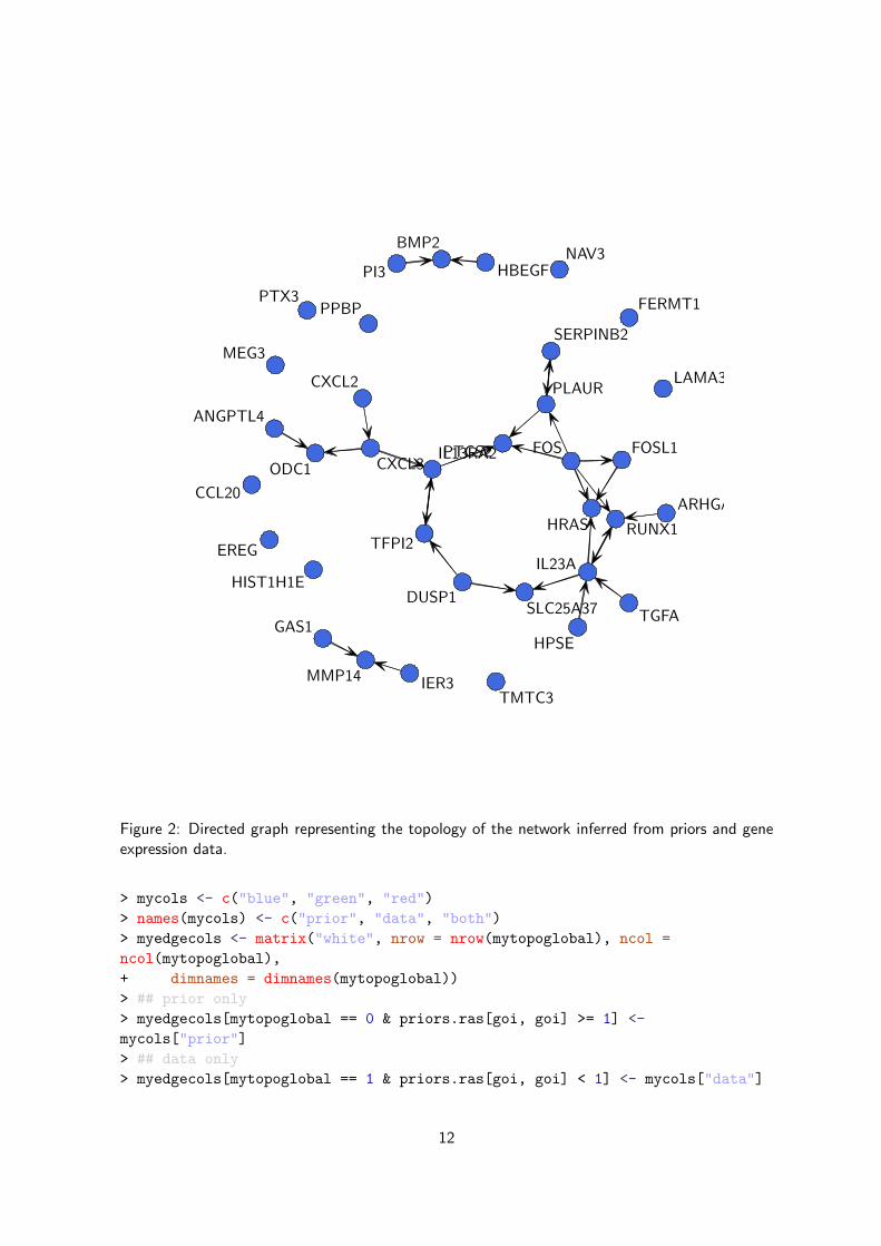
A quick look at the topology in Figure 2 allows us to identify IL13RA2 as a highly connected gene.By searching for these two genes in GeneSigDB7, a manually curated database of published genesignatures developed by Dr Aedin Culhane, we can see that IL13RA2, in addition to be includedin the RAS signature published in [Bild et al., 2006], is also part of other signatures publishedin colon, leukemia, ovarian and stomach cancers. Receptors for interleukin-13 (IL-13R) are over-expressed on several types of solid cancers; it is not only associated with colon cancer, but alsowith many other cancers including colon cancer [Niranjan et al., 2008].

Question: How many of the inferred interactions were not known beforehand (not in the priors)?

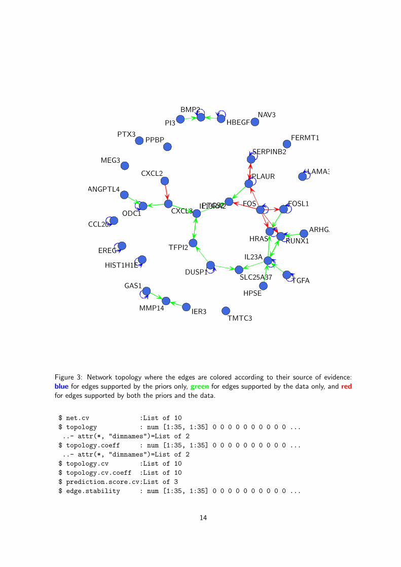
We could also highlight the interactions that were already known (blue), the new interactionssupported by the gene expression (green) and the interactions both known and supported by thedata (red), see Figure 3.

> ## preparing colors

6http://www.cytoscape.org/7http://compbio.dfci.harvard.edu/genesigdb/

11

http://www.cytoscape.org/

http://compbio.dfci.harvard.edu/genesigdb/

FOS

CCL20

PPBP

HRAS

DUSP1

GAS1

CXCL3IL13RA2PTGS2

TFPI2

BMP2NAV3

HBEGF

HIST1H1E

ARHGAP27

TGFA

EREG

IER3

ODC1

IL23A

PLAUR

FERMT1

LAMA3

SERPINB2

TMTC3

ANGPTL4

MEG3

HPSE

SLC25A37

FOSL1

PI3

PTX3

MMP14

RUNX1

CXCL2

Figure 2: Directed graph representing the topology of the network inferred from priors and geneexpression data.

> mycols <- c("blue", "green", "red")

> names(mycols) <- c("prior", "data", "both")

> myedgecols <- matrix("white", nrow = nrow(mytopoglobal), ncol =

ncol(mytopoglobal),

+ dimnames = dimnames(mytopoglobal))

> ## prior only

> myedgecols[mytopoglobal == 0 & priors.ras[goi, goi] >= 1] <-

mycols["prior"]

> ## data only

> myedgecols[mytopoglobal == 1 & priors.ras[goi, goi] < 1] <- mycols["data"]

12

> ## both in priors and data

> myedgecols[mytopoglobal == 1 & priors.ras[goi, goi] >= 1] <- mycols["both"]

> mytopoglobal2 <- (myedgecols != "white") + 0


> xnet2 <- network(x = mytopoglobal2, matrix.type = "adjacency",

+ directed = TRUE, loops = TRUE, vertex.attrnames =

dimnames(mytopoglobal2)[[1]])

> plot.network(x = xnet2, displayisolates = TRUE, displaylabels = TRUE,

+ boxed.labels = FALSE, label.pos = 0, arrowhead.cex = 1.5,

+ vertex.cex = 2, vertex.col = "royalblue", jitter = FALSE,

+ pad = 0.5, edge.col = myedgecols, coord = mynetlayout)

In Figure 3 we can see that all the interactions included in the priors have been also supported bythe data (red) and have been inferred in the final network; only the self loops (blue), which arenot allowed by our regression-based network inference method, have been discarded. Many newinteractions (green) have been inferred from the gene expression data.

Although of interest, the topology does not tell us much about the quality of the network inference.Therefore we implemented two statistics to help us focus on the gene interactions that are wellsupported by the data:

• edge-specific stability,

• gene-specific prediction score.

The idea is to use a cross-validation procedure8 to infer multiple networks from different trainingdatasets to assess both the stability of the inference and its predictive ability. The functionnetinf.cv, although computationally intensive, is doing all the work for us. The vast majorityof the parameters are the same than for the netinf function, with some additions such as nfoldthat is the number of folds for the cross-validation procedure.

> myres.cv <- netinf.cv(data = data.ras[, goi], categories = 3,

+ priors = priors.ras[goi, goi], maxparents = 3, priors.weight = 0.5,

+ method = "regrnet", nfold = 10, seed = 54321)

Question: Do you know why netinf.cv takes longer to compute than netinf?

The object myres.cv contains a lot of information related to the network inference process:

> print(str(myres.cv, 1))

List of 9

$ net :List of 4

8http://en.wikipedia.org/wiki/Cross-validation_(statistics)

13

http://en.wikipedia.org/wiki/Cross-validation_(statistics)

FOS

CCL20

PPBP

HRAS

DUSP1

GAS1

CXCL3IL13RA2PTGS2

TFPI2

BMP2NAV3

HBEGF

HIST1H1E

ARHGAP27

TGFA

EREG

IER3

ODC1

IL23A

PLAUR

FERMT1

LAMA3

SERPINB2

TMTC3

ANGPTL4

MEG3

HPSE

SLC25A37

FOSL1

PI3

PTX3

MMP14

RUNX1

CXCL2

Figure 3: Network topology where the edges are colored according to their source of evidence:blue for edges supported by the priors only, green for edges supported by the data only, and redfor edges supported by both the priors and the data.

$ net.cv :List of 10

$ topology : num [1:35, 1:35] 0 0 0 0 0 0 0 0 0 0 ...

..- attr(*, "dimnames")=List of 2

$ topology.coeff : num [1:35, 1:35] 0 0 0 0 0 0 0 0 0 0 ...


$ topology.cv :List of 10

$ topology.cv.coeff :List of 10

$ prediction.score.cv:List of 3

$ edge.stability : num [1:35, 1:35] 0 0 0 0 0 0 0 0 0 0 ...

14


$ edge.stability.cv : num [1:35, 1:35] 0 0 0 0 0 0 0 0 0 0 ...


NULL

with

net Model object of the network inferred using the entire dataset.

net.cv List of models network models fitted at each fold of the cross-validation.

topology Topology of the model inferred using the entire dataset.

topology.coeff coefficients of each local linear regression model fitted using the entire dataset.

topology.cv Topology of the networks inferred at each fold of the cross-validation.

topology.coeff coefficients of each local linear regression model fitted at each fold of the cross-validation.

prediction.score.cv List of prediction scores (R2, NRMSE , MCC) computed at each fold ofthe cross-validation.

edge.stability Stability of the edges inferred during cross-validation; only the stability of theedges present in the network inferred using the entire dataset is reported.

edge.stability.cv Stability of the edges inferred during cross-validation.

We can now extract these statistics to better quantify the robustness of the network inference.

3.3 Edge-specific stability

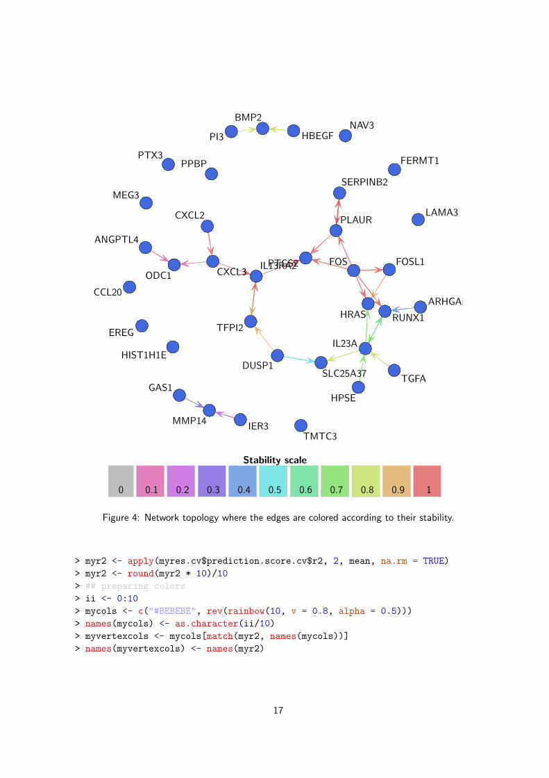
At each fold of the cross-validation, a network is inferred using a slightly different dataset. Thisvariation in the set of observations used to fit the network model induces some variation at thelevel of the inference. Some edges may be poorly supported by the data and therefore theirinference strongly depends on the training dataset and is not generalizable. Since we performeda 10-fold cross-validation, we can calculate for each edge the frequency of its presence in theinferred networks, the most robust edge being inferred 10 times, the less robust ones only once ortwice.

Let’s display the topology of the network inferred from the entire dataset where the edges arecolored according to their stability (Figure 4).


> ii <- 0:10

> mycols <- c("#BEBEBE", rev(rainbow(10, v = 0.8, alpha = 0.5)))

> names(mycols) <- as.character(ii/10)

> myedgecols <- matrix("#00000000", nrow = nrow(mytopoglobal),

+ ncol = ncol(mytopoglobal), dimnames = dimnames(mytopoglobal))

> for (k in 1:length(mycols)) {

+ myedgecols[myres.cv$edge.stability == names(mycols)[k]] <- mycols[k]

15

+ }

> myedgecols[!mytopoglobal] <- "#00000000"

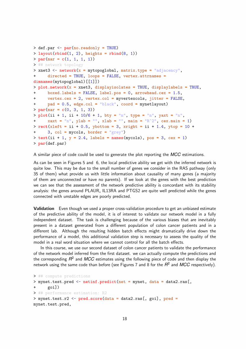
> def.par <- par(no.readonly = TRUE)

> layout(rbind(1, 2), heights = rbind(8, 1))

> par(mar = c(1, 1, 1, 1))


> xnet3 <- network(x = mytopoglobal, matrix.type = "adjacency",






+ pad = 0.5, edge.col = myedgecols, coord = mynetlayout)

> par(mar = c(0, 3, 1, 3))

> plot(ii + 1, ii + 10/6 + 1, bty = "n", type = "n", yaxt = "n",

+ xaxt = "n", ylab = "", xlab = "", main = "Stability scale",

+ cex.main = 1)

> rect(xleft = ii + 0.5, ybottom = 3, xright = ii + 1.4, ytop = 10 +

+ 3, col = mycols, border = "grey")

> text(ii + 1, y = 2.4, labels = names(mycols), pos = 3, cex = 1)

> par(def.par)

As can be seen, the inference of more than half of the edges is very stable, especially around thehighly connected genes, that are IL13RA2, PLAUR, PTGS2, FOS. However the inference of theinteractions with PPBP is unstable.

3.4 Gene-specific prediction score

Since our regression-based network inference approach actually fits local regression models toassess the dependence between the parent genes and the target/child gene, we can actuallyquantify the strength of this dependence by assessing the predictive ability of the network modelfor each individual gene. Several performance criteria have been implemented so far:

• R2: proportion of variance of the target/child gene explained by the regression model. Thevalue lies in {0, 1}, the larger, the better.

• NRMSE : normalized root mean squared error of the regression model. The values are > 0,the lower, the better.

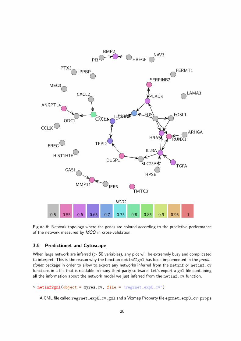
• MCC: Matthews correlation coefficient (also called multi-class correlation). This is a perfor-mance criterion widely used in the classification framework so it requires first a discretizationof the gene expression data in classes (this is done implicitly by the functions netinf.cv

and pred.score). The value lies in {0, 1}, the larger, the better.

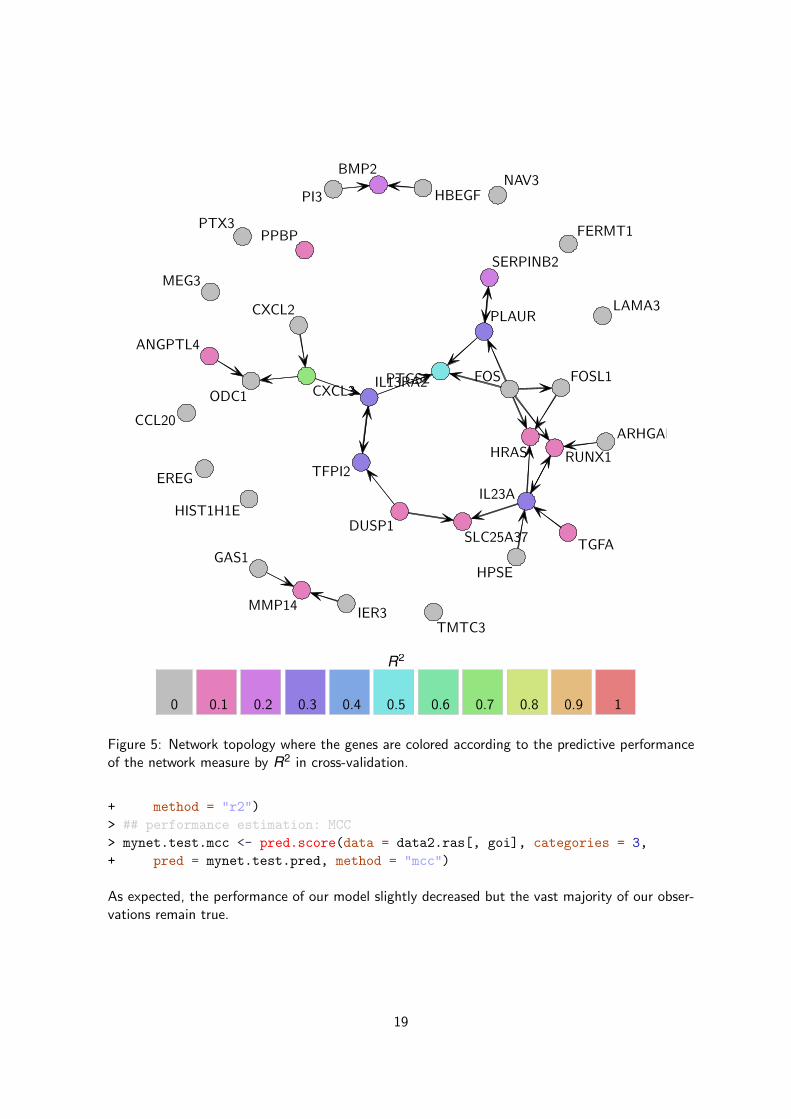
Let’s focus on R2 and MCC. We can easily display the topology by coloring nodes according tothe predictive ability of the network estimated by R2 (Figure 5) and MCC (Figure 6). Here is thecode for generating the plot reporting the R2 estimations:

16

FOS

CCL20

PPBP

HRAS

DUSP1

GAS1

CXCL3IL13RA2PTGS2

TFPI2

BMP2NAV3

HBEGF

HIST1H1E

ARHGAP27

TGFA

EREG

IER3

ODC1

IL23A

PLAUR

FERMT1

LAMA3

SERPINB2

TMTC3

ANGPTL4

MEG3

HPSE

SLC25A37

FOSL1

PI3

PTX3

MMP14

RUNX1

CXCL2

Stability scale

0 0.1 0.2 0.3 0.4 0.5 0.6 0.7 0.8 0.9 1

Figure 4: Network topology where the edges are colored according to their stability.

> myr2 <- apply(myres.cv$prediction.score.cv$r2, 2, mean, na.rm = TRUE)

> myr2 <- round(myr2 * 10)/10


> ii <- 0:10

> mycols <- c("#BEBEBE", rev(rainbow(10, v = 0.8, alpha = 0.5)))

> names(mycols) <- as.character(ii/10)

> myvertexcols <- mycols[match(myr2, names(mycols))]

> names(myvertexcols) <- names(myr2)

17


> layout(rbind(1, 2), heights = rbind(8, 1))

> par(mar = c(1, 1, 1, 1))


> xnet3 <- network(x = mytopoglobal, matrix.type = "adjacency",





+ vertex.cex = 2, vertex.col = myvertexcols, jitter = FALSE,

+ pad = 0.5, edge.col = "black", coord = mynetlayout)

> par(mar = c(0, 3, 1, 3))

> plot(ii + 1, ii + 10/6 + 1, bty = "n", type = "n", yaxt = "n",

+ xaxt = "n", ylab = "", xlab = "", main = "R^2", cex.main = 1)

> rect(xleft = ii + 0.5, ybottom = 3, xright = ii + 1.4, ytop = 10 +

+ 3, col = mycols, border = "grey")

> text(ii + 1, y = 2.4, labels = names(mycols), pos = 3, cex = 1)

> par(def.par)

A similar piece of code could be used to generate the plot reporting the MCC estimations.

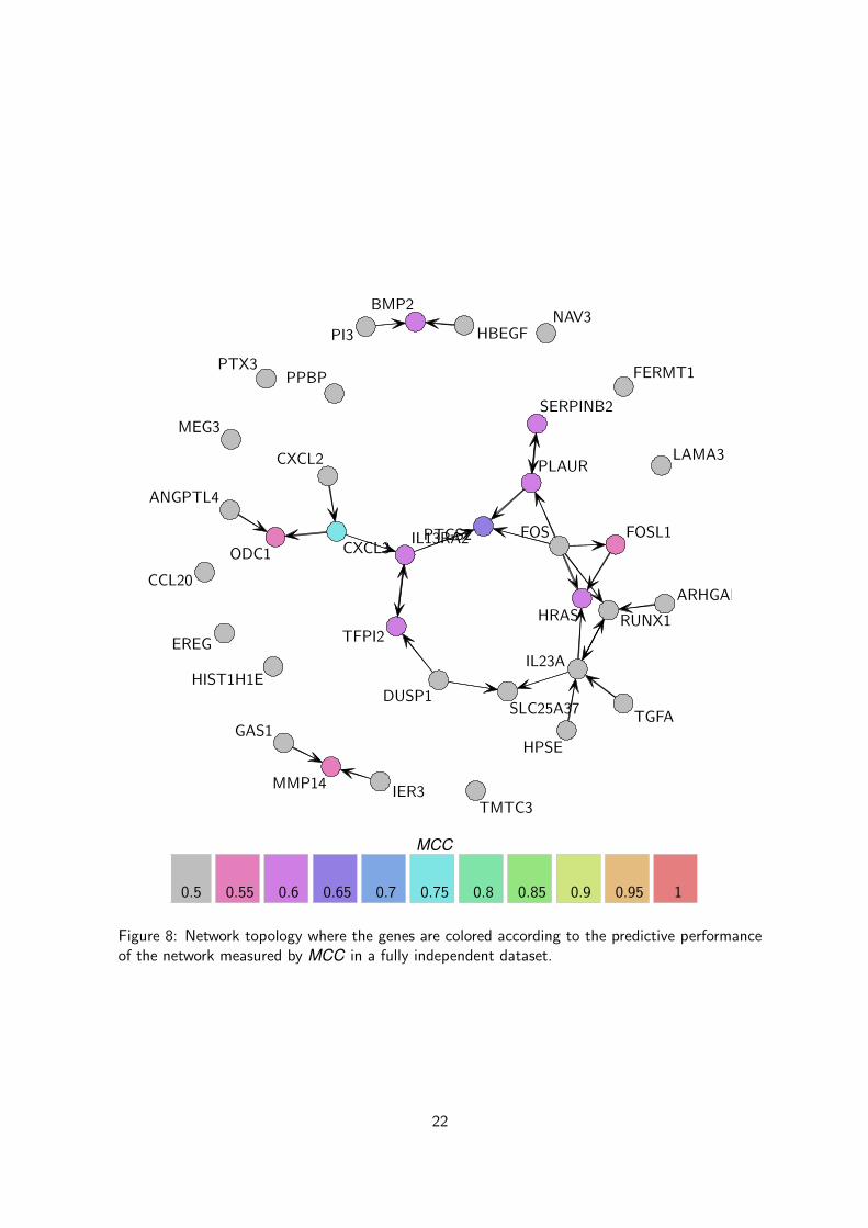
As can be seen in Figures 5 and 6, the local predictive ability we get with the inferred network isquite low. This may be due to the small number of genes we consider in the RAS pathway (only35 of them) what provide us with little information about causality of many genes (a majorityof them are unconnected or have no parents). If we look at the genes with the best predictionwe can see that the assessment of the network predictive ability is concordant with its stabilityanalysis: the genes around PLAUR

”IL13RA and PTGS2 are quite well predicted while the genes

connected with unstable edges are poorly predicted.

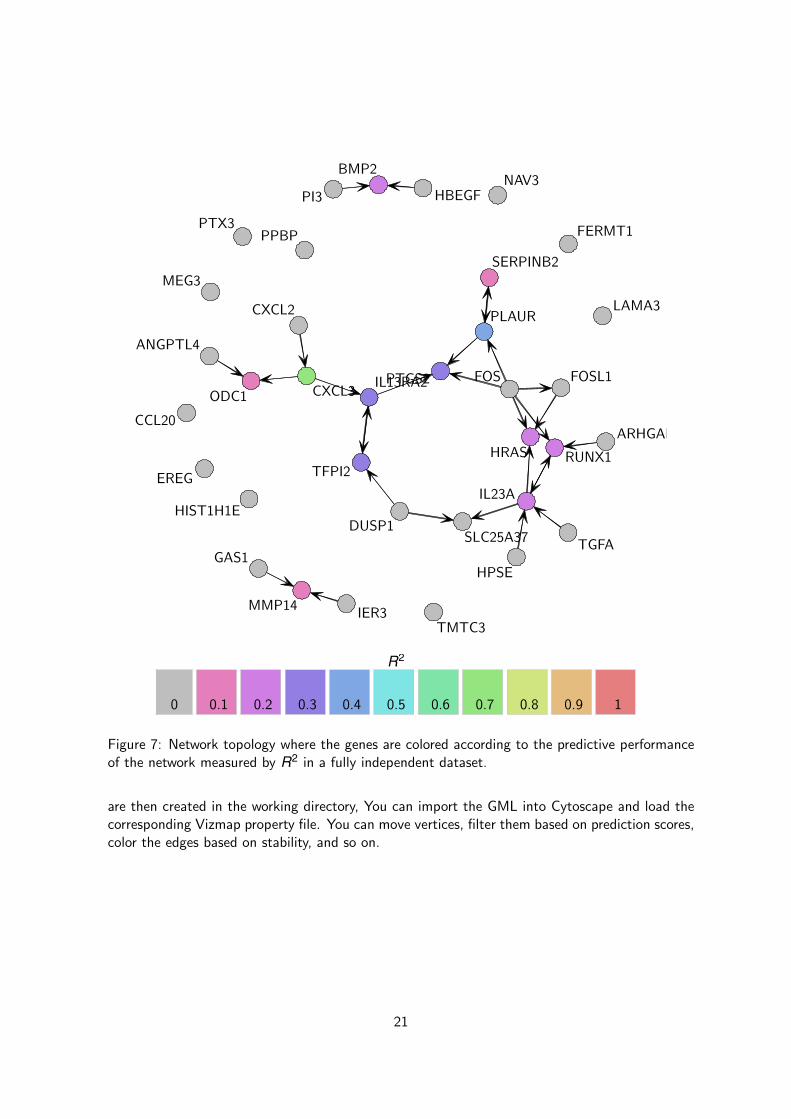
Validation Even though we used a proper cross-validation procedure to get an unbiased estimateof the predictive ability of the model, it is of interest to validate our network model in a fullyindependent dataset. The task is challenging because of the various biases that are inevitablypresent in a dataset generated from a different population of colon cancer patients and in adifferent lab. Although the resulting hidden batch effects might dramatically drive down theperformance of a model, this additional validation step is necessary to assess the quality of themodel in a real word situation where we cannot control for all the batch effects.

In this course, we use our second dataset of colon cancer patients to validate the performanceof the network model inferred from the first dataset. we can actually compute the predictions andthe corresponding R2 and MCC estimates using the following piece of code and then display thenetwork using the same code than before (see Figures 7 and 8 for the R2 and MCC respectively).

> ## compute predictions

> mynet.test.pred <- netinf.predict(net = mynet, data = data2.ras[,

+ goi])

> ## performance estimation: R2

> mynet.test.r2 <- pred.score(data = data2.ras[, goi], pred =

mynet.test.pred,

18

FOS

CCL20

PPBP

HRAS

DUSP1

GAS1

CXCL3IL13RA2PTGS2

TFPI2

BMP2NAV3

HBEGF

HIST1H1E

ARHGAP27

TGFA

EREG

IER3

ODC1

IL23A

PLAUR

FERMT1

LAMA3

SERPINB2

TMTC3

ANGPTL4

MEG3

HPSE

SLC25A37

FOSL1

PI3

PTX3

MMP14

RUNX1

CXCL2

R2

0 0.1 0.2 0.3 0.4 0.5 0.6 0.7 0.8 0.9 1

Figure 5: Network topology where the genes are colored according to the predictive performanceof the network measure by R2 in cross-validation.

+ method = "r2")

> ## performance estimation: MCC

> mynet.test.mcc <- pred.score(data = data2.ras[, goi], categories = 3,

+ pred = mynet.test.pred, method = "mcc")

As expected, the performance of our model slightly decreased but the vast majority of our obser-vations remain true.

19

FOS

CCL20

PPBP

HRAS

DUSP1

GAS1

CXCL3IL13RA2PTGS2

TFPI2

BMP2NAV3

HBEGF

HIST1H1E

ARHGAP27

TGFA

EREG

IER3

ODC1

IL23A

PLAUR

FERMT1

LAMA3

SERPINB2

TMTC3

ANGPTL4

MEG3

HPSE

SLC25A37

FOSL1

PI3

PTX3

MMP14

RUNX1

CXCL2

MCC

0.5 0.55 0.6 0.65 0.7 0.75 0.8 0.85 0.9 0.95 1

Figure 6: Network topology where the genes are colored according to the predictive performanceof the network measured by MCC in cross-validation.

3.5 Predictionet and Cytoscape

When large network are inferred (> 50 variables), any plot will be extremely busy and complicatedto interpret, This is the reason why the function netinf2gml has been implemented in the predic-tionet package in order to allow to export any networks inferred from the netinf or netinf.cvfunctions in a file that is readable in many third-party software. Let’s export a gml file containingall the information about the network model we just inferred from the netinf.cv function.

> netinf2gml(object = myres.cv, file = "regrnet_expO_cv")

A CML file called regrnet_expO_cv.gml and a Vizmap Property file egrnet_expO_cv.props

20

FOS

CCL20

PPBP

HRAS

DUSP1

GAS1

CXCL3IL13RA2PTGS2

TFPI2

BMP2NAV3

HBEGF

HIST1H1E

ARHGAP27

TGFA

EREG

IER3

ODC1

IL23A

PLAUR

FERMT1

LAMA3

SERPINB2

TMTC3

ANGPTL4

MEG3

HPSE

SLC25A37

FOSL1

PI3

PTX3

MMP14

RUNX1

CXCL2

R2

0 0.1 0.2 0.3 0.4 0.5 0.6 0.7 0.8 0.9 1

Figure 7: Network topology where the genes are colored according to the predictive performanceof the network measured by R2 in a fully independent dataset.

are then created in the working directory, You can import the GML into Cytoscape and load thecorresponding Vizmap property file. You can move vertices, filter them based on prediction scores,color the edges based on stability, and so on.

21

FOS

CCL20

PPBP

HRAS

DUSP1

GAS1

CXCL3IL13RA2PTGS2

TFPI2

BMP2NAV3

HBEGF

HIST1H1E

ARHGAP27

TGFA

EREG

IER3

ODC1

IL23A

PLAUR

FERMT1

LAMA3

SERPINB2

TMTC3

ANGPTL4

MEG3

HPSE

SLC25A37

FOSL1

PI3

PTX3

MMP14

RUNX1

CXCL2

MCC

0.5 0.55 0.6 0.65 0.7 0.75 0.8 0.85 0.9 0.95 1

Figure 8: Network topology where the genes are colored according to the predictive performanceof the network measured by MCC in a fully independent dataset.

22

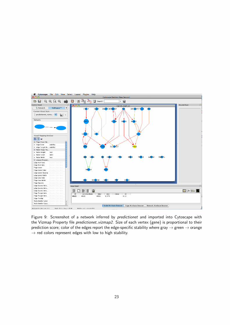
Figure 9: Screenshot of a network inferred by predictionet and imported into Cytoscape withthe Vizmap Property file predictionet vizmap2. Size of each vertex (gene) is proportional to theirprediction score; color of the edges report the edge-specific stability where gray→ green→ orange→ red colors represent edges with low to high stability.

23

4 Comparison of network inference with respect to the priors

Based on our approach to quantify the stability and predictive ability of a gene interaction network,we are now able to statistically compare the performance of two or more networks. This networkmodel selection could help us optimize a parameter such as the weight of the priors during thenetwork inference (priors.weight) or identify the best method of network inference (Bayesianvs regression-based network inference for instance).

Let’s infer and compare the prediction scores (estimated in cross-validation) of five networks withpriors.weight = 0, 0.25, 0.5, 0.75 and 1.

> ## priors.weight 0

> myres.cv.pw0 <- netinf.cv(data = data.ras[, goi], categories = 3,

+ priors = priors.ras[goi, goi], maxparents = 3, priors.weight = 0,


> ## priors.weight 0.25





> myres.cv.pw050 <- myres.cv







+ priors = priors.ras[goi, goi], maxparents = 3, priors.weight = 1,


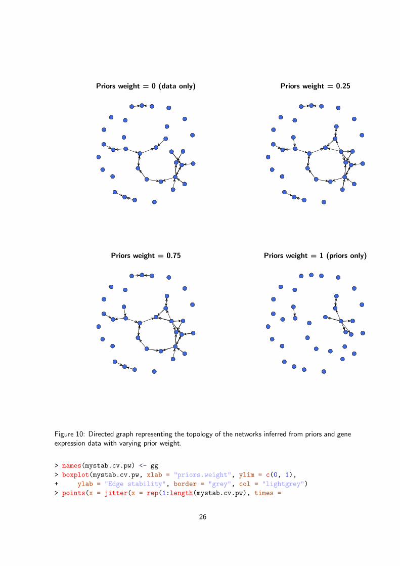
Now let’s display the topology of the networks we just inferred by varying the weight we put onthe priors (see Figure 10).


> layout(mat = matrix(1:4, nrow = 2, ncol = 2, byrow = TRUE))


> mytopot <- net2topo(net = myres.cv.pw0$net)

> xnett <- network(x = mytopot, matrix.type = "adjacency", directed = TRUE,

+ loops = FALSE, vertex.attrnames = dimnames(mytopot)[[1]])

> plot.network(x = xnett, displayisolates = TRUE, displaylabels = FALSE,



+ pad = 0.5, edge.col = "black", coord = mynetlayout, main = "Priors

weight = 0 (data only)")




24






weight = 0.25")









weight = 0.75")









weight = 1 (priors only)")

> par(def.par)

As can be seen in Figure 10, the networks generated from data only (priors.weight = 0) andfrom priors only (priors.weight = 1) are very sparse, and the combination of priors and dataenables the identification of more gene interactions. But a denser topology does not imply thatall the inferred interactions are well supported by the data. In order to select the best network(s)we can statistically compare their stability and predictive ability.

4.1 Comparison of edge-specific prediction scores

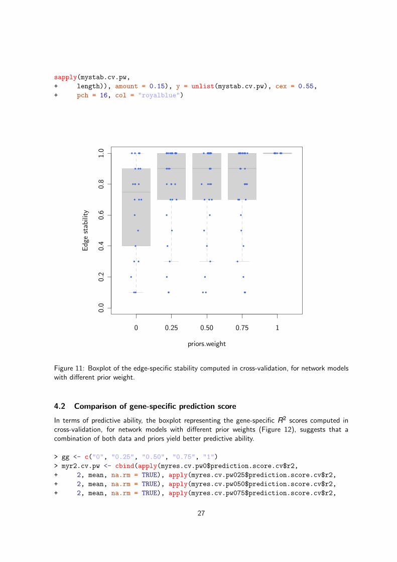
In order to compare the stability of the network inference, we can draw a boxplot representingthe edge-specific stability of the network inference with respect to the weight put on the priors(Figure 11). As expected, the network inferred from priors only is perfectly stable (the inferencedoes not depend on the data anymore) but what is interesting is the gain in stability when thepriors are used as compared to networks inferred from data alone.

> gg <- c("0", "0.25", "0.50", "0.75", "1")

> mystab.cv.pw <- list(myres.cv.pw0$edge.stability[myres.cv.pw0$topology ==

+ 1], myres.cv.pw025$edge.stability[myres.cv.pw025$topology ==




+ 1])

25

Priors weight = 0 (data only) Priors weight = 0.25

Priors weight = 0.75 Priors weight = 1 (priors only)

Figure 10: Directed graph representing the topology of the networks inferred from priors and geneexpression data with varying prior weight.

> names(mystab.cv.pw) <- gg

> boxplot(mystab.cv.pw, xlab = "priors.weight", ylim = c(0, 1),

+ ylab = "Edge stability", border = "grey", col = "lightgrey")

> points(x = jitter(x = rep(1:length(mystab.cv.pw), times =

26

sapply(mystab.cv.pw,

+ length)), amount = 0.15), y = unlist(mystab.cv.pw), cex = 0.55,

+ pch = 16, col = "royalblue")

0 0.25 0.50 0.75 1

0.0

0.2

0.4

0.6

0.8

1.0

priors.weight

Ed

gest

abili

ty

Figure 11: Boxplot of the edge-specific stability computed in cross-validation, for network modelswith different prior weight.

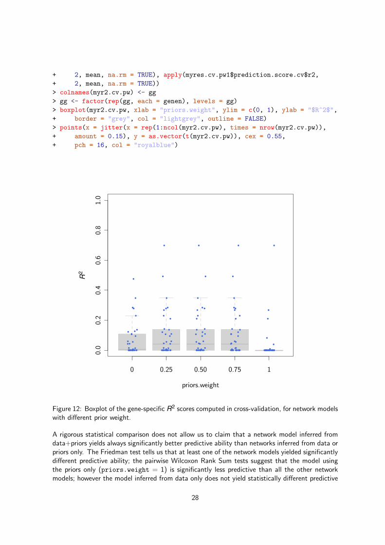
4.2 Comparison of gene-specific prediction score

In terms of predictive ability, the boxplot representing the gene-specific R2 scores computed incross-validation, for network models with different prior weights (Figure 12), suggests that acombination of both data and priors yield better predictive ability.

> gg <- c("0", "0.25", "0.50", "0.75", "1")

> myr2.cv.pw <- cbind(apply(myres.cv.pw0$prediction.score.cv$r2,

+ 2, mean, na.rm = TRUE), apply(myres.cv.pw025$prediction.score.cv$r2,



27


+ 2, mean, na.rm = TRUE))

> colnames(myr2.cv.pw) <- gg

> gg <- factor(rep(gg, each = genen), levels = gg)

> boxplot(myr2.cv.pw, xlab = "priors.weight", ylim = c(0, 1), ylab = "$R^2$",

+ border = "grey", col = "lightgrey", outline = FALSE)

> points(x = jitter(x = rep(1:ncol(myr2.cv.pw), times = nrow(myr2.cv.pw)),

+ amount = 0.15), y = as.vector(t(myr2.cv.pw)), cex = 0.55,


0 0.25 0.50 0.75 1

0.0

0.2

0.4

0.6

0.8

1.0

priors.weight

R2

Figure 12: Boxplot of the gene-specific R2 scores computed in cross-validation, for network modelswith different prior weight.

A rigorous statistical comparison does not allow us to claim that a network model inferred fromdata+priors yields always significantly better predictive ability than networks inferred from data orpriors only. The Friedman test tells us that at least one of the network models yielded significantlydifferent predictive ability; the pairwise Wilcoxon Rank Sum tests suggest that the model usingthe priors only (priors.weight = 1) is significantly less predictive than all the other networkmodels; however the model inferred from data only does not yield statistically different predictive

28

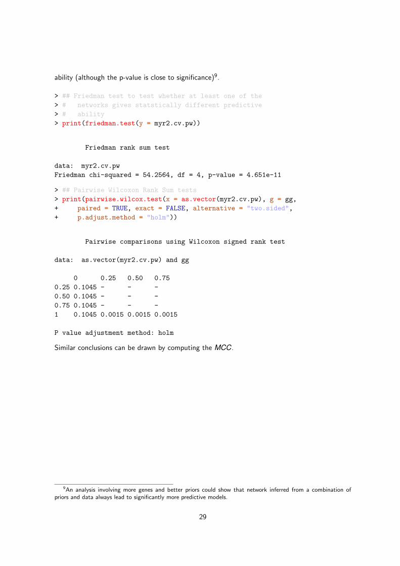
ability (although the p-value is close to significance)9.

> ## Friedman test to test whether at least one of the

> # networks gives statstically different predictive

> # ability

> print(friedman.test(y = myr2.cv.pw))

Friedman rank sum test

data: myr2.cv.pw

Friedman chi-squared = 54.2564, df = 4, p-value = 4.651e-11

> ## Pairwise Wilcoxon Rank Sum tests

> print(pairwise.wilcox.test(x = as.vector(myr2.cv.pw), g = gg,

+ paired = TRUE, exact = FALSE, alternative = "two.sided",

+ p.adjust.method = "holm"))

Pairwise comparisons using Wilcoxon signed rank test

data: as.vector(myr2.cv.pw) and gg

0 0.25 0.50 0.75

0.25 0.1045 - - -

0.50 0.1045 - - -

0.75 0.1045 - - -

1 0.1045 0.0015 0.0015 0.0015

P value adjustment method: holm

Similar conclusions can be drawn by computing the MCC.

9An analysis involving more genes and better priors could show that network inferred from a combination ofpriors and data always lead to significantly more predictive models.

29

5 Comparison of network inference with respect to the trainingdata

To identify the parts of the networks where interactions are well supported by the data we es-timated in cross-validation edge-specific stabilities and gene-specific prediction scores of a givennetwork model. Ultimately these statistics should help us identify the parts of the network thatare generalizable, whose inference does not strongly depend on the dataset used as training set.

Inference of generalizable network models is a challenging task because of the various biasesthat are inevitably present in datasets generated from different populations of cancer patientsand in different labs. Therefore the resulting hidden batch effects might dramatically affect theinference of a network model.

Let’s use expO.colon.ras dataset as training set to infer our network model (use data onlyfor inference, priors.weight=0). Now we will use our second dataset, jorissen.colon.ras,to infer another network model (use data only for inference, priors.weight=0) and comparethem to test whether the network inference strongly depend on the training set or not.

First infer a network from expO.colon.ras and jerissen.colon.ras datasets separately.

> ## expO

> myres21.cv <- netinf.cv(data = data.ras[, goi], categories = 3,

+ priors = priors2.ras[goi, goi], maxparents = 3, priors.weight = 0,


> ## jorissen

> myres22.cv <- netinf.cv(data = data2.ras[, goi], categories = 3,

+ priors = priors2.ras[goi, goi], maxparents = 3, priors.weight = 0,


Let’s display the topologies of the networks inferred from these two datasets. As can be seenin Figure 13, approximately half of the interactions are inferred in both datasets.

> topo1 <- net2topo(net = myres21.cv$net)

> topo2 <- net2topo(net = myres22.cv$net)


> myedgecols <- matrix("white", nrow = nrow(topo1), ncol = ncol(topo1),

+ dimnames = dimnames(topo1))

> myedgecols[topo1 == 1 & topo2 == 1 & priors.ras[rownames(topo1),

+ colnames(topo1)] > 0] <- "orange"

> myedgecols[topo1 == 1 & topo2 == 1 & priors.ras[rownames(topo1),

+ colnames(topo1)] <= 0] <- "red"



> ## expO

> mycolt <- myedgecols

> mycolt[myedgecols == "white" & topo1 == 1] <- "black"

> xnett <- network(x = topo1, matrix.type = "adjacency", directed = TRUE,



30



+ pad = 0.5, edge.col = mycolt, coord = mynetlayout, main = "Dataset:

expO.colon.ras")

> ## jorissen

> mycolt <- myedgecols

> mycolt[myedgecols == "white" & topo2 == 1] <- "black"

> xnett <- network(x = topo2, matrix.type = "adjacency", directed = TRUE,





+ pad = 0.5, edge.col = mycolt, coord = mynetlayout, main = "Dataset:

jorissen.colon.ras")

> par(def.par)

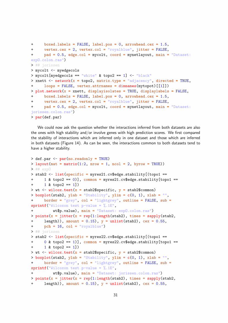
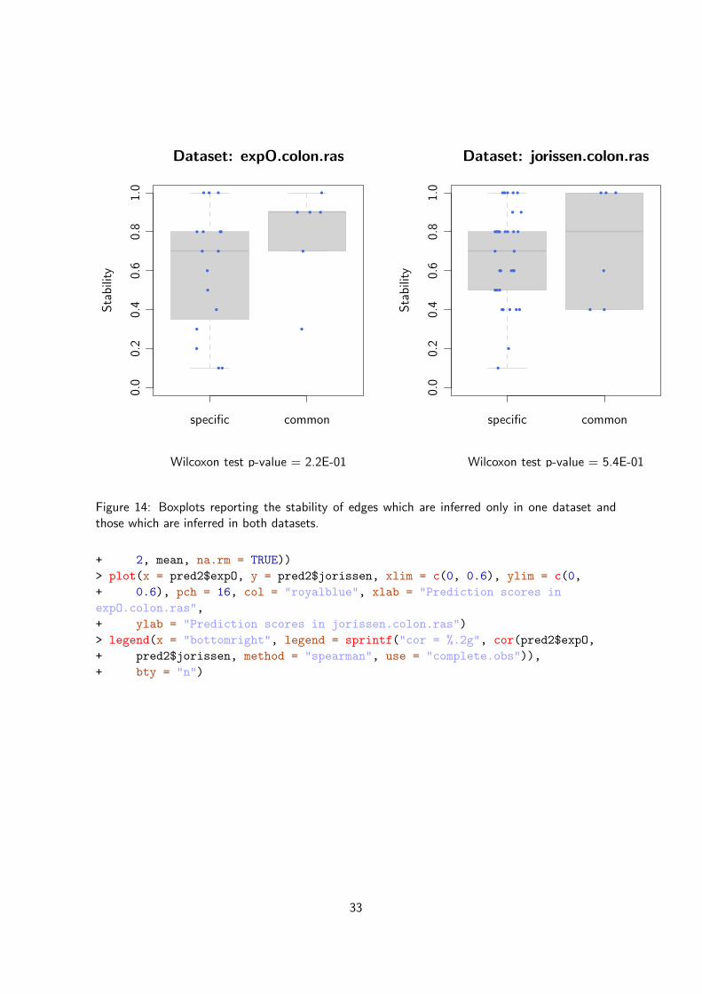
We could now ask the question whether the interactions inferred from both datasets are alsothe ones with high stability and/or involve genes with high prediction scores. We first comparedthe stability of interactions which are inferred only in one dataset and those which are inferredin both datasets (Figure 14). As can be seen, the interactions common to both datasets tend tohave a higher stability.



> ## expO

> stab2 <- list(specific = myres21.cv$edge.stability[(topo1 ==

+ 1 & topo2 == 0)], common = myres21.cv$edge.stability[topo1 ==

+ 1 & topo2 == 1])

> wt <- wilcox.test(x = stab2$specific, y = stab2$common)

> boxplot(stab2, ylab = "Stability", ylim = c(0, 1), xlab = "",

+ border = "grey", col = "lightgrey", outline = FALSE, sub =

sprintf("Wilcoxon test p-value = %.1E",

+ wt$p.value), main = "Dataset: expO.colon.ras")

> points(x = jitter(x = rep(1:length(stab2), times = sapply(stab2,

+ length)), amount = 0.15), y = unlist(stab2), cex = 0.55,


> ## jorissen

> stab2 <- list(specific = myres22.cv$edge.stability[(topo1 ==

+ 0 & topo2 == 1)], common = myres22.cv$edge.stability[topo1 ==

+ 1 & topo2 == 1])

> wt <- wilcox.test(x = stab2$specific, y = stab2$common)

> boxplot(stab2, ylab = "Stability", ylim = c(0, 1), xlab = "",

+ border = "grey", col = "lightgrey", outline = FALSE, sub =

sprintf("Wilcoxon test p-value = %.1E",

+ wt$p.value), main = "Dataset: jorissen.colon.ras")

> points(x = jitter(x = rep(1:length(stab2), times = sapply(stab2,

+ length)), amount = 0.15), y = unlist(stab2), cex = 0.55,

31

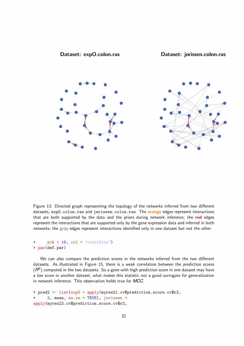
Dataset: expO.colon.ras Dataset: jorissen.colon.ras

Figure 13: Directed graph representing the topology of the networks inferred from two differentdatasets, expO.colon.ras and jerissen.colon.ras. The orange edges represent interactionsthat are both supported by the data and the priors during network inference; the red edgesrepresent the interactions that are supported only by the gene expression data and inferred in bothnetworks; the gray edges represent interactions identified only in one dataset but not the other.


> par(def.par)

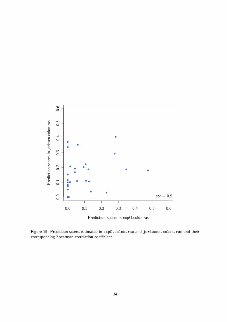
We can also compare the prediction scores in the networks inferred from the two differentdatasets. As illustrated in Figure 15, there is a weak correlation between the prediction scores(R2) computed in the two datasets. So a gene with high prediction score in one dataset may havea low score in another dataset, what makes this statistic not a good surrogate for generalizationin network inference. This observation holds true for MCC.

> pred2 <- list(expO = apply(myres21.cv$prediction.score.cv$r2,

+ 2, mean, na.rm = TRUE), jorissen =

apply(myres22.cv$prediction.score.cv$r2,

32

specific common

0.0

0.2

0.4

0.6

0.8

1.0

Dataset: expO.colon.ras

Wilcoxon test p-value = 2.2E-01

Sta

bili

ty

specific common0.

00.

20.

40.

60.

81.

0

Dataset: jorissen.colon.ras

Wilcoxon test p-value = 5.4E-01

Sta

bili

ty

Figure 14: Boxplots reporting the stability of edges which are inferred only in one dataset andthose which are inferred in both datasets.

+ 2, mean, na.rm = TRUE))

> plot(x = pred2$expO, y = pred2$jorissen, xlim = c(0, 0.6), ylim = c(0,

+ 0.6), pch = 16, col = "royalblue", xlab = "Prediction scores in

expO.colon.ras",

+ ylab = "Prediction scores in jorissen.colon.ras")

> legend(x = "bottomright", legend = sprintf("cor = %.2g", cor(pred2$expO,

+ pred2$jorissen, method = "spearman", use = "complete.obs")),

+ bty = "n")

33

0.0 0.1 0.2 0.3 0.4 0.5 0.6

0.0

0.1

0.2

0.3

0.4

0.5

0.6

Prediction scores in expO.colon.ras

Pre

dic

tion

scor

esin

jori

ssen

.col

on.r

as

cor = 0.5

Figure 15: Prediction scores estimated in expO.colon.ras and jorissen.colon.ras and theircorresponding Spearman correlation coefficient.

34

6 Future works

The Predictive Networks web application and the predictionet R package that we are usingtoday are currently under active development and new features will be introduced progressively.Here is a list of the major features that will included soon:

• Predictive Networks web application:

– Option to filter gene interactions according to their domain (e.g., colon cancer).

• predictionet R package:

– Development of a novel approach to improve the completeness of the inferred network(and so get a more biological meaningful network) and its predictive ability. The ideabehind this ensemble network inference method is to generate many different networksthat are equally well supported by the data and combine them in a consensus networkinstead of a single (local) optimum.

35

Session Info

• R version 2.13.0 (2011-04-13), x86_64-apple-darwin9.8.0

• Base packages: base, datasets, grDevices, graphics, methods, splines, stats, tools, utils

• Other packages: Rcpp 0.9.4, cacheSweave 0.4-5, catnet 1.10.0, codetools 0.2-8,filehash 2.1-1, formatR 0.2-1, getopt 1.16, highlight 0.2-5, igraph 0.5.5-2, network 1.6,optparse 0.9.1, parser 0.0-13, penalized 0.9-35, pgfSweave 1.2.1, predictionet 0.9,stashR 0.3-3, survival 2.36-9, tikzDevice 0.6.1

• Loaded via a namespace (and not attached): digest 0.4.2

36

References

Learning Bayesian Networks. Prentica Hall, 2003.

A. H. Bild, G. Yao, J. T. Chang, Q. Wang, A. Potti, D. Chasse, M-B. Joshi, >D. Harpole, J. M.Lancaster, A. Berschuk, J. A. Olson Jr, J. R. Marks, H. K. Dressman, M. West, and J. R. Nevins.Oncogenic pathway signatures in human cancers as a guide to targeted therapies. Nature, 439:353–356, 2006.

Jie Cheng, Russell Greiner, Jonathan Kelly, David Bell, and Weiru Liu. Learning bayesian net-works from data: An information-theory based approach. Artificial Intelligence, 137(1-2):43– 90, 2002. ISSN 0004-3702. URL http://www.sciencedirect.com/science/article/

B6TYF-45BCRWV-2/2/390d83eb89efc5e0bc8de9e43e0681d9.

Chris Ding and Hanchuan Peng. Minimum redundancy feature selection from microarray geneexpression data. J Bioinform Comput Biol, 3(2):185–205, Apr 2005.

Robert N Jorissen, Peter Gibbs, Michael Christie, Saurabh Prakash, Lara Lipton, Jayesh Desai,David Kerr, Lauri A Aaltonen, Diego Arango, Mogens Kruhøffer, Torben F Orntoft, Claus Lind-bjerg Andersen, Mike Gruidl, Vidya P Kamath, Steven Eschrich, Timothy J Yeatman, andOliver M Sieber. Metastasis-associated gene expression changes predict poor outcomes in pa-tients with dukes stage b and c colorectal cancer. Clin Cancer Res, 15(24):7642–7651, Dec2009. doi: 10.1158/1078-0432.CCR-09-1431.

Matthew N McCall, Benjamin M Bolstad, and Rafael A Irizarry. Frozen robust multiarray analysis(frma). Biostatistics, 11(2):242–53, Apr 2010. doi: 10.1093/biostatistics/kxp059.

Patrick E Meyer, Kevin Kontos, Frederic Lafitte, and Gianluca Bontempi. Information-theoreticinference of large transcriptional regulatory networks. EURASIP J Bioinform Syst Biol, page79879, 2007. doi: 10.1155/2007/79879.

Patrick Emmanual Meyer. Information-Theoretic Variable Selection and Network Inference fromMicroarray Data. PhD thesis, Universite Libre de Bruxelles, December 2008.

V Niranjan, R Mahmood, A kalaivan, and Sudha S. Study of cancer gene in x-chromosome.Journal of Theoretical and Applied Information Technology, 4(1):31–55, 2008.

C. Olsen, P. E. Meyer, and G. Bontempi. Inferring causal relationships using information-theoreticmeasures. In Proceedings of the 5th Benelux Bioinformatics Conference (BBC09), 2009.

C W Reuter, M A Morgan, and L Bergmann. Targeting the ras signaling pathway: a rational,mechanism-based treatment for hematologic malignancies? Blood, 96(5):1655–69, Sep 2000.

Michael E Smoot, Keiichiro Ono, Johannes Ruscheinski, Peng-Liang Wang, and Trey Ideker.Cytoscape 2.8: new features for data integration and network visualization. Bioinformatics, 27(3):431–2, Feb 2011. doi: 10.1093/bioinformatics/btq675.

37

http://www.sciencedirect.com/science/article/B6TYF-45BCRWV-2/2/390d83eb89efc5e0bc8de9e43e0681d9

http://www.sciencedirect.com/science/article/B6TYF-45BCRWV-2/2/390d83eb89efc5e0bc8de9e43e0681d9

Documents

R/Bioconductor course Predictive Networks: a new · PDF fileR/Bioconductor course Predictive Networks: a new framework for ... Harvard School of ... Erik Bakke, James Hardwick, Gianluca