RBF-PS scheme for solving the equal width equation

Applied Mathematics and Computation 222 (2013) 619–631

Contents lists available at ScienceDirect

Applied Mathematics and Computation

journal homepage: www.elsevier .com/ locate/amc

RBF-PS scheme for solving the equal width equation

0096-3003/$ - see front matter � 2013 Elsevier Inc. All rights reserved.http://dx.doi.org/10.1016/j.amc.2013.07.031

E-mail address: [email protected]

Marjan UddinDepartment of Basic Sciences and Islamiat, University of Engineering and Technology, Peshawar, Pakistan

a r t i c l e i n f o a b s t r a c t

Keywords:Radial kernelsMeshless techniqueRBF-PS schemeEqual width equation

The equal width equation is solved by a RBF-PS scheme. This technique is meshless, andthere is no need to linearize the nonlinear terms. The radial kernels are used to transformthe PDE into a system of ODEs. A higher order ODE solver is used to solve the ODE system.The method is tested for single solitary wave, interaction of two and three solitary waves,the development of an undular bore and the interaction of two solitary waves. The resultsare compared with earlier work and other methods.

� 2013 Elsevier Inc. All rights reserved.

1. Introduction

The equal width (EW) equation

ut þ uux � luxxt ¼ 0; x 2 ½a; b�; t > 0; ð1Þ

where l is a real constant and the subscripts represent differentiation, e.g. ut ¼ @u=@t. The equal width (EW) equation wassuggested by Morrison et al. [37], which is used to model waves generated in a shallow water channel. This equation rep-resents an alternative to the well-known regularized long wave (RLW) equation. For a smooth function uðx; tÞ on a domain½a; b� � ½0; t� the given model has an analytic solution that is a traveling single solitary wave

uðx; tÞ ¼ 3Csech2ðk½x� x0 � Ct�Þ; ð2Þ

where k ¼ 1=ffiffiffiffiffiffiffi4l

p, but generally numerical methods have to be used for the solution of the given model. The boundary con-

ditions uð�1Þ ¼ 0 are imposed because the given model has a traveling wave solution, moves with constant speed C andvanishes at x ¼ �1.

The EW equation has been solved analytically for a limited set of boundary and initial conditions. As a result, a large num-ber of numerical techniques has been developed to solve the equation. For example Gardner et al. [23] applied cubic B-splinefinite elements to simulate the motion and interaction of the solitary waves for the EW equation. Garcia et al. [24] used a spec-tral method for solving the EW equation. Archilla [3] introduced a numerical method for the EW equation using a spectralFourier discretization for the spatial derivatives. Gardner et al. [22] investigated the motion of solitary waves and the devel-opment of an undular bore by a Petrov Galerkin method using quadratic B-spline spatial finite elements. Khalifa and Raslan[32] proposed a finite difference technique combined with the invariant imbedding method to describe the migration of a sin-gle solitary wave and the evolution of a Maxwellian initial condition for the EW equation. Zaki [56] solved the EW equation bya least-squares technique using linear space–time finite elements to examine the motion of a single solitary wave and thedevelopment of an undular bore. Zaki [57] also studied the development of a train of EW solitary waves induced by boundaryforcing using a Petrov–Galerkin finite-element scheme with test functions taken as quadratic B-splines. Raslan [38] used acollocation method based on quintic B-spline finite elements to represent the amplitude, position and velocity of a single sol-itary wave, the interaction of solitary waves and the development of an undular bore. Dag and Saka [8] used a cubic B-spline

http://crossmark.dyndns.org/dialog/?doi=10.1016/j.amc.2013.07.031&domain=pdf

http://dx.doi.org/10.1016/j.amc.2013.07.031

mailto:[email protected]

http://dx.doi.org/10.1016/j.amc.2013.07.031

http://www.sciencedirect.com/science/journal/00963003

http://www.elsevier.com/locate/amc

620 M. Uddin / Applied Mathematics and Computation 222 (2013) 619–631

collocation method and studied the development of the undular bore and generation of the waves for the EW equation. Dogan[13] solved the EW equation by Galerkin’s method using linear finite elements. Raslan [39] studied the numerical solution ofthe EW equation by a collocation method using quartic B-splines. Esen [14] used a Galerkin method with quadratic B-splinefinite elements for the numerical solution of the EW equation. Esen et al. [15] applied a linearized implicit-difference methodfor solving the EW equation. Ali [2] solved the EW equation numerically by spectral based on chebyshev polynomials. Sakaet al. [42,43] solved numerically the EW equation by three different numerical methods.

The meshless methods are based on interpolating functions expressed entirely in terms of nodes [5]. During the past twodecades the meshless methods have been developed and effectively applied to solve many engineering and science problems[1,4,12,16,18,33,35]. There is a class of meshless methods that focus on the use of radial basis functions [6], such as radial basisfunction collocation method (RBFCM) [21,28,29,50–53]. The radial basis functions (RBFs) have been under intensive researchin multivariate data and Kansa used them for scattered data approximation in [29] and pioneered the solution of PDEs [30];that is why the method is some times called the Kansa’s method. The key point of Kansa’s method for solving the PDEs is theapproximation of the fields on the boundary and in the domain by a set of global approximation functions. The convergencetheory of Kansa’s approach was provided by Schaback [44–46]. The main advantage of using the RBFCM for solution of PDEs isits simplicity, applicability to various PDEs, and effectiveness in dealing with high dimensional problems and complicated do-mains. The main disadvantage of RBFCM comes from the related full matrices that are very sensitive to the choice of the freeparameter in RBFs and difficult to solve for problems with a large number of unknowns. This is because the use of the radialbasis function interpolation increases the condition numbers of the related matrices with increasing number of nodes. This isespecially true for a bad choice of data centers and when infinitely smooth basic functions such as multiquadrics are used withextreme values of their associated shape parameter. There are several methods to circumvent this issue such as domaindecomposition [25,31] the greedy algorithm [27,34], etc. One of the possibilities for mitigating computational cost forlarge-scale problems is to employ the domain decomposition by Mai-Duy and Tran-Cong [36], the multi-grid approach andcompactly supported RBFs by Chen et al. [7] in 2002, and local radial basis function method [48], etc

Fasshauer [17] connected the radial basis functions collocation method to the pseudo-spectral method, known as RBF-PSmethod. Fasshauer used the RBF-PS method for solving the Allen–Cahn equation, 2D Helmholtz equation and 2D Laplaceequation with piecewise boundary conditions [18]. Ferreira et al. [19,20] used the RBF-PS method for analyzing beams, platesand shells problems. Roque et al. [40,41] applied the RBF-PS method for composite and sandwich plates problems, and Mar-jan Uddin et al. [54,55] applied RBF-PS method for solving some wave-type PDEs.

In the present work we extended the approach of Fasshauer [17] and developed a numerical scheme for the EW equation.

2. RBF-PS method

Given a set of centers fx1; . . . ; xNg � X. The RBF approximation to Eq. (1) takes the form

uðx; tÞ ¼XN

j¼1

kjðtÞKðx; xjÞ; x 2 X; ð3Þ

where the radial kernel K is defined as Kðx; xjÞ : /ðkx� xjkÞ;1 6 j 6 N, and r ¼ kx� xjk denotes the Euclidean distance be-tween two points x and xj and /ðrÞ is a function defined for r P 0. Interpolation of the function u : X! R on the set of pointsfx1; . . . ; xNg is done by solving the system of equations

uðxi; tÞ ¼XN

j¼1

kjðtÞKðxi; xjÞ; 1 6 i 6 N: ð4Þ

In matrix form, we have

u ¼ Ak; ð5Þ

where the entries of the matrix A are Kðxi; xjÞ;1 6 i; j 6 N, and the vector of expansion coefficients is k ¼ ½k1; k2; . . . ; kN�T .Using Eq. (1) the derivatives ux may be obtained by differentiating the kernel functions and then evaluating at each pointxi;1 6 i 6 N; we have in matrix–vector notation

ux ¼ Axk; ð6Þ

where the entries of the matrix Ax are ddx Kðx; xjÞx¼xi

;1 6 i; j 6 N. The differentiation matrix can be obtained by solving equa-tions (5) and (6) for the value of k. Thus, we have

ux ¼ AxA�1u ¼ Dxu; ð7Þ

where Dx ¼ AxA�1 is the differentiation matrix. It should be noted that the differentiation matrix depends on the invertibil-ity of the matrix A. It is well known that the matrix A is always invertible for distinct set of collocation points. In a similarway, we can write

uxx ¼ AxxA�1u ¼ Dxxu; ð8Þ

M. Uddin / Applied Mathematics and Computation 222 (2013) 619–631 621

where Dxx ¼ AxxA�1 and the entries of matrix Axx are d2

dx2 Kðx; xjÞx¼xi;1 6 i; j 6 N.

Similarly, we can compute differentiation matrices of higher order.Using the above differentiation matrices, the numerical scheme corresponding to Eqs. (1) is given as

u0 þ u � ðDxuÞ � lDxxu0 ¼ 0: ð9Þ

This equation may be written as

ðI� lDxxÞu0 ¼ �ðu � ðDxuÞÞ: ð10Þ

The matrix B ¼ ðI� lDxxÞ is time-independent. We can compute the pseudo-inverse By of B; hence, we have

u0 ¼ Du; ð11Þ

where D ¼ �ByðdiagðuÞDxÞ. Eq. (11) is of the form

u0 ¼ FðuÞ: ð12Þ

This is the ODE system generated by the present scheme. To discretize in time we can use any ODE solver like ode113, ode45from Matlab. The starting vector will be the initial solution u0.

ode45 is based on an explicit Runge–Kutta (4) and (5) formula, the Dormand-Prince pair [11]. It is a one-step solver forcomputing uðtnÞ, and it needs only the solution at the immediately preceding time point, uðtn�1Þ. In general, ode45 is the bestfunction to apply as a first try for most problems.

ode113 is a variable order Adams–Bashforth–Moulton PECE solver [47]. It may be more efficient than ode45 for stringenttolerances and when the ODE file function is particularly expensive to evaluate. ode113 is a multistep solver; it normallyrequires the solution at several preceding time points to compute the current solution.

A good ODE solver will automatically select a reasonable time step dt and detect stiffness of the ODE system. For this ODEcomputation we have also used a fourth-order Runge–Kutta method and selected the time step dt manually.

r1 ¼ FðunÞ;

r2 ¼ F uþ dt2

r1

� �;

r3 ¼ F uþ dt2

r2

� �;

r4 ¼ Fðuþ dtr3Þ;

unþ1 ¼ un þ dt6ðr1 þ 2r2 þ 2r3 þ r4Þ:

ð13Þ

In the present method the differentiation matrices Dx, Dxx, are computed only once outside the time-stepping procedure.Inside the time-stepping we require only matrix–vector multiplications. So, this approach is much faster than the approachused in [26,10,9], where the interpolation coefficients are computed at each time-step.

We can choose any twice differentiable kernel function which decays toward infinity. In order to make the matrices A;Dx

and Dxx sparse, we can use compactly supported radial kernel functions.A variety of kernel functions are available in the literature. In our computation we used the the multiquadrics

(/ðrÞ ¼ffiffiffiffiffiffiffiffiffiffiffiffiffiffiffir2 þ c2p

) and the Wendland (/3;2ðrÞ ¼ ð1� crÞ6þð35ðcrÞ2 þ 18cr þ 3Þ) RBFs. As usual these RBFs contain a shapeparameter c. For these types of meshless methods an algorithm for choosing the good value of shape parameter is proposedby Fasshauer [18].

2.1. Stability analysis

In the present technique the time-dependent PDE is transformed into a system of ODEs in time. The method of lines refersto the idea of solving the coupled system of ODEs by a finite difference method in t (e.g Runge–Kutta, etc.). The numericalstability of the method of lines is investigated by a rule of rhumb. The method of lines is stable if the eigenvalues of the (line-arized) spatial discretization operator, scaled by dt, lie in the stability region of the time-discretization operator, [49].

The stability region is a part of a complex plane consisting of those eigenvalues for which the technique produce abounded solution. In the present meshless method of lines our numerical scheme is given in (11). We investigate the stableand unstable eigenvalue spectrum for the EW equation by computing the eigenvalues of the matrix D, scaled by dt.

2.2. Choosing a good value of shape parameter

Many radial kernel functions contain a free shape parameter and solution accuracy greatly depends on this parameter. Forimproved accuracy, the user has to choose an optimal value of the shape parameter. In this paper we used the criteria pro-posed by Fasshauer [18] for a good value of the shape parameter.

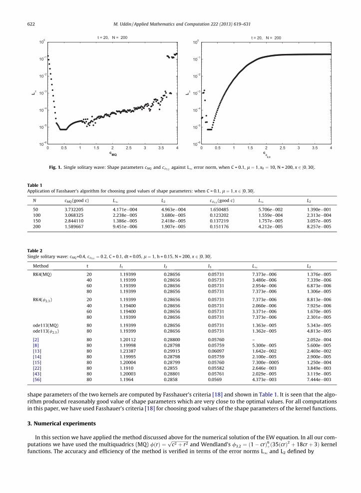
In solving single solitary wave problems, the values of the shape parameters of the Multiquadrics (MQ) and Wendland’scompactly supported kernel /2;3 are plotted against the L1 error norm which are shown in Fig. 1, while the good values of the

0 0.5 1 1.5 2 2.5 3 3.5 410−6

10−5

10−4

10−3

10−2

10−1

100

cMQ

L∞

t = 20, N = 200

0 0.5 1 1.5 2 2.5 3 3.5 410−6

10−5

10−4

10−3

10−2

10−1

100

cφ2,3

L∞

t = 20, N = 200

Fig. 1. Single solitary wave: Shape parameters cMQ and c/3;2 against L1 error norm, when C = 0.1, l ¼ 1; x0 ¼ 10, N = 200, x 2 ½0;30�.

Table 1Application of Fasshauer’s algorithm for choosing good values of shape parameters: when C = 0.1, l ¼ 1; x 2 ½0;30�.

N cMQ (good c) L1 L2 c/3;2(good c) L1 L2

50 3.732205 4.171e�004 4.963e�004 1.650485 5.706e�002 1.390e�001100 3.068325 2.238e�005 3.680e�005 0.123202 1.559e�004 2.313e�004150 2.844110 1.386e�005 2.418e�005 0.137219 1.757e�005 3.057e�005200 1.589667 9.451e�006 1.907e�005 0.151176 4.212e�005 8.257e�005

Table 2Single solitary wave: cMQ =0.4, c/3;2 ¼ 0:2, C = 0.1, dt = 0.05, l ¼ 1, h = 0.15, N = 200, x 2 ½0;30�.

Method t I1 I2 I3 L1 L2

RK4(MQ) 20 1.19399 0.28656 0.05731 7.373e�006 1.376e�00540 1.19399 0.28656 0.05731 3.480e�006 7.339e�00660 1.19399 0.28656 0.05731 2.954e�006 6.873e�00680 1.19399 0.28656 0.05731 7.373e�006 1.306e�005

RK4(/2;3) 20 1.19399 0.28656 0.05731 7.373e�006 8.813e�00640 1.19400 0.28656 0.05731 2.060e�006 7.925e�00660 1.19400 0.28656 0.05731 3.371e�006 1.670e�00580 1.19399 0.28656 0.05731 7.373e�006 2.301e�005

ode113(MQ) 80 1.19399 0.28656 0.05731 1.363e�005 5.343e�005ode113(/2;3) 80 1.19399 0.28656 0.05731 1.362e�005 4.813e�005

[2] 80 1.20112 0.28800 0.05760 – 2.052e�004[8] 80 1.19998 0.28798 0.05759 5.300e�005 5.600e�005[13] 80 1.23387 0.29915 0.06097 1.642e�002 2.469e�002[14] 80 1.19995 0.28798 0.05759 2.100e�005 2.900e�005[15] 80 1.20004 0.28799 0.05760 7.300e�0005 1.250e�004[22] 80 1.1910 0.2855 0.05582 2.646e�003 3.849e�003[43] 80 1.20003 0.28801 0.05761 2.029e�005 3.119e�005[56] 80 1.1964 0.2858 0.0569 4.373e�003 7.444e�003


shape parameters of the two kernels are computed by Fasshauer’s criteria [18] and shown in Table 1. It is seen that the algo-rithm produced reasonably good value of shape parameters which are very close to the optimal values. For all computationsin this paper, we have used Fasshauer’s criteria [18] for choosing good values of the shape parameters of the kernel functions.

3. Numerical experiments

In this section we have applied the method discussed above for the numerical solution of the EW equation. In all our com-putations we have used the multiquadrics (MQ) /ðrÞ ¼

ffiffiffiffiffiffiffiffiffiffiffiffiffiffiffic2 þ r2p

and Wendland’s /3;2 ¼ ð1� crÞ6þð35ðcrÞ2 þ 18cr þ 3Þ kernelfunctions. The accuracy and efficiency of the method is verified in terms of the error norms L1 and L2 defined by

−8 −6 −4 −2 0 2 4x 10−5

10−14

10−12

10−10

10−8

10−6

10−4

10−2 L∞ = 4.4601e−005, t = 2, cMQ = 1.5897

x

y

Scaled eigenvalues of D

−3 −2.5 −2 −1.5 −1 −0.5 0 0.5−3

−2

−1

0

1

2

3 L∞ = 4.4601e−005, t = 2, cMQ = 1.5897

x

y

Region of stability of RK4 schemeScaled eigenvalues of D

0 5 10 15 20 25 300

0.05

0.1

0.15

0.2

0.25

0.3

0.35t = 2, cMQ = 1.5897

x

u

Exact solutionNumerical solution

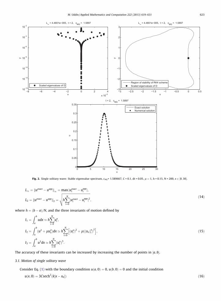
Fig. 2. Single solitary wave: Stable eigenvalue spectrum, cMQ = 1.589667, C = 0.1, dt = 0.05, l ¼ 1, h = 0.15, N = 200, x 2 ½0;30�.


L1 ¼ kuexact � uappk1 ¼max juexacti � uapp

i j;

L2 ¼ kuexact � uappk2 ¼

ffiffiffiffiffiffiffiffiffiffiffiffiffiffiffiffiffiffiffiffiffiffiffiffiffiffiffiffiffiffiffiffiffiffiffiffiffiffiffihXN

i¼0

juexacti � uapp

i j2

vuut ;ð14Þ

where h ¼ ðb� aÞ=N, and the three invariants of motion defined by

I1 ¼Z b

audx ’ h

XN

i¼0

uni ;

I2 ¼Z b

aðu2 þ lu2

x Þdx ’ hXN

i¼0

ðuni Þ

2 þ lððuxÞni Þ2

h i;

I3 ¼Z b

au3dx ’ h

XN

i¼0

ðuni Þ

3:

ð15Þ

The accuracy of these invariants can be increased by increasing the number of points in ½a; b�.

3.1. Motion of single solitary wave

Consider Eq. (1) with the boundary condition uða;0Þ ¼ 0, uðb;0Þ ¼ 0 and the initial condition

uðx;0Þ ¼ 3Csech2ðk½x� x0�Þ ð16Þ

−0.05 0 0.05 0.1 0.15 0.2 0.25 0.3 0.3510−12

10−10

10−8

10−6

10−4

10−2 L∞ = 0.2901, t = 2, cMQ = 10

x

y

Scaled eigenvalues of D

−3 −2.5 −2 −1.5 −1 −0.5 0 0.5−3

−2

−1

0

1

2

3 L∞ = 0.2901, t = 2, cMQ = 10

x

y

Stabilty region of RK4Scaled eigenvalues of D

0 5 10 15 20 25 30−0.05

0

0.05

0.1

0.15

0.2

0.25

0.3t = 2, cMQ = 10

x

u

Nuemerical solutionExact solution

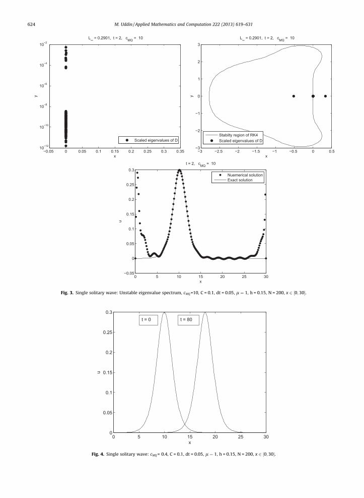
Fig. 3. Single solitary wave: Unstable eigenvalue spectrum, cMQ =10, C = 0.1, dt = 0.05, l ¼ 1, h = 0.15, N = 200, x 2 ½0;30�.

0 5 10 15 20 25 300

0.05

0.1

0.15

0.2

0.25

0.3

x

u

t = 0 t = 80

Fig. 4. Single solitary wave: cMQ = 0.4, C = 0.1, dt = 0.05, l ¼ 1, h = 0.15, N = 200, x 2 ½0;30�.


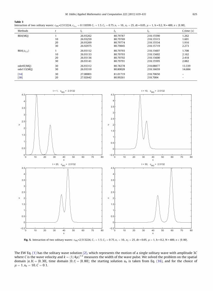
Table 3Interaction of two solitary waves: cMQ =2.513224, c/3;2 ¼ 0:118599 C1 ¼ 1:5;C2 ¼ 0:75; x1 ¼ 10., x2 ¼ 25, dt = 0.05, l ¼ 1, h = 0.2, N = 400, x 2 ½0;80�.

Methods t I1 I2 I3 C.time (s)

RK4(MQ) 1 26.93262 80.79787 218.15590 1.26210 26.93259 80.79769 218.15515 1.60120 26.93269 80.79774 218.15534 1.91630 26.92975 80.79845 218.15719 2.273

RK4(/3;2) 1 26.93152 80.79793 218.15607 1.70810 26.93133 80.79793 218.15602 2.16220 26.93136 80.79792 218.15600 2.41830 26.93141 80.79791 218.15595 2.882

ode45(MQ) 30 26.93312 80.78278 218.08877 13.339ode113(MQ) 30 26.93310 80.80028 218.16659 14.684

[14] 30 27.00003 81.01719 218.70650 –[38] 20 27.02642 80.99261 218.7004 –

0 10 20 30 40 50 60 70 800

0.5

1

1.5

2

2.5

3

3.5

4

4.5t = 1, cMQ = 2.5132

x

u

0 10 20 30 40 50 60 70 80−0.5

0

0.5

1

1.5

2

2.5

3

3.5

4

4.5t = 10, cMQ = 2.5132

x

u

0 10 20 30 40 50 60 70 80−0.5

0

0.5

1

1.5

2

2.5

3

3.5

4

4.5t = 20, cMQ = 2.5132

x

u

0 10 20 30 40 50 60 70 80−0.5

0

0.5

1

1.5

2

2.5

3

3.5

4

4.5t = 30, cMQ = 2.5132

x

u

Fig. 5. Interaction of two solitary waves: cMQ =2.513224, C1 ¼ 1:5;C2 ¼ 0:75; x1 ¼ 10., x2 ¼ 25, dt = 0.05, l ¼ 1, h = 0.2, N = 400, x 2 ½0;80�.


The EW Eq. (1) has the solitary wave solution (2), which represents the motion of a single solitary wave with amplitude 3Cwhere C is the wave velocity and k ¼ ð1=4lÞ1=2 measures the width of the wave pulse. We solved the problem on the spatialdomain ½a; b� ¼ ½0;30�, time domain ½0; t� ¼ ½0;80�; the starting solution u0 is taken from Eq. (16), and for the choice ofl ¼ 1; x0 ¼ 10;C ¼ 0:1.

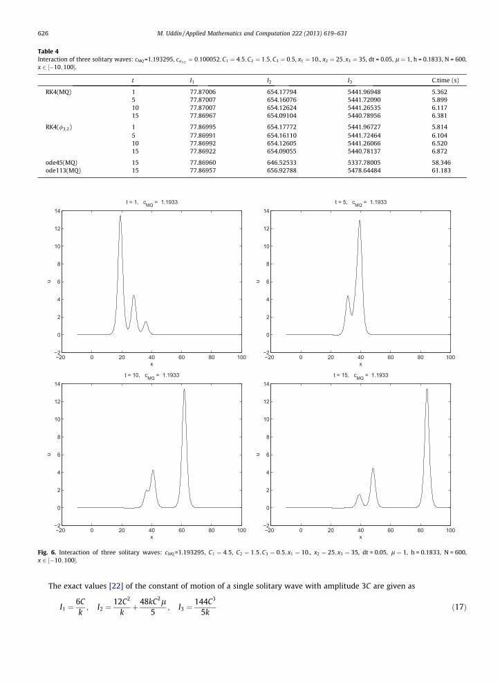
Table 4Interaction of three solitary waves: cMQ =1.193295, c/3;2 ¼ 0:100052;C1 ¼ 4:5;C2 ¼ 1:5;C3 ¼ 0:5, x1 ¼ 10., x2 ¼ 25; x3 ¼ 35, dt = 0.05, l ¼ 1, h = 0.1833, N = 600,x 2 ½�10;100�.

t I1 I2 I3 C.time (s)

RK4(MQ) 1 77.87006 654.17794 5441.96948 5.3625 77.87007 654.16076 5441.72090 5.89910 77.87007 654.12624 5441.26535 6.11715 77.86967 654.09104 5440.78956 6.381

RK4(/3;2) 1 77.86995 654.17772 5441.96727 5.8145 77.86991 654.16110 5441.72464 6.10410 77.86992 654.12605 5441.26066 6.52015 77.86922 654.09055 5440.78137 6.872

ode45(MQ) 15 77.86960 646.52533 5337.78005 58.346ode113(MQ) 15 77.86957 656.92788 5478.64484 61.183

−20 0 20 40 60 80 100−2

0

2

4

6

8

10

12

14t = 1, cMQ = 1.1933

x

u

−20 0 20 40 60 80 100−2

0

2

4

6

8

10

12

14t = 5, cMQ = 1.1933

x

u

−20 0 20 40 60 80 100−2

0

2

4

6

8

10

12

14t = 10, cMQ = 1.1933

x

u

−20 0 20 40 60 80 100−2

0

2

4

6

8

10

12

14t = 15, cMQ = 1.1933

x

u

Fig. 6. Interaction of three solitary waves: cMQ =1.193295, C1 ¼ 4:5, C2 ¼ 1:5;C3 ¼ 0:5; x1 ¼ 10., x2 ¼ 25; x3 ¼ 35, dt = 0.05, l ¼ 1, h = 0.1833, N = 600,x 2 ½�10;100�.


The exact values [22] of the constant of motion of a single solitary wave with amplitude 3C are given as

I1 ¼6Ck; I2 ¼

12C2

kþ 48kC2l

5; I3 ¼

144C3

5kð17Þ

−20 −10 0 10 20 30 40 500

0.02

0.04

0.06

0.08

0.1

0.12

0.14

0.16

0.18

0.2

t = 200, cφ3,2

= 0.10006

x

u

−20 −10 0 10 20 30 40 500

0.02

0.04

0.06

0.08

0.1

0.12

0.14

0.16

0.18

0.2

t = 400, cφ3,2

= 0.10006

x

u

−20 −10 0 10 20 30 40 500

0.02

0.04

0.06

0.08

0.1

0.12

0.14

0.16

0.18

0.2

t = 600, cφ3,2

= 0.10006

x

u

−20 −10 0 10 20 30 40 500

0.02

0.04

0.06

0.08

0.1

0.12

0.14

0.16

0.18

0.2

t = 800, cφ3,2

= 0.10006

x

u

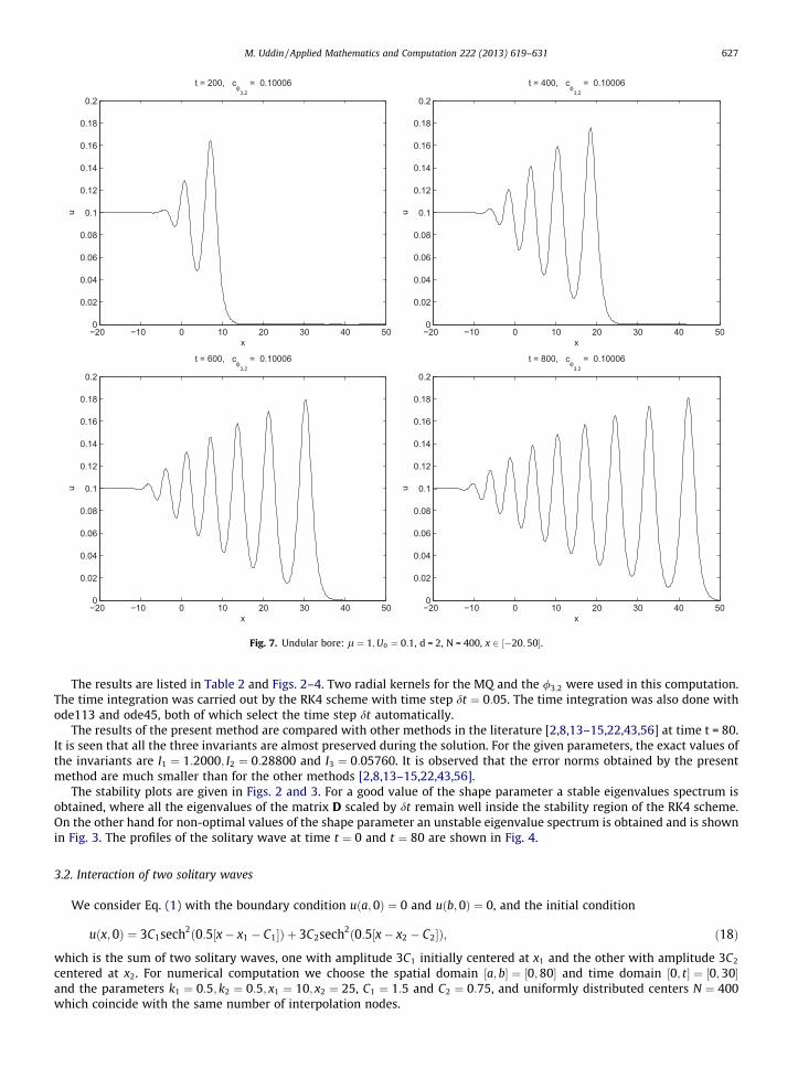
Fig. 7. Undular bore: l ¼ 1;U0 ¼ 0:1, d = 2, N = 400, x 2 ½�20;50�.


The results are listed in Table 2 and Figs. 2–4. Two radial kernels for the MQ and the /3;2 were used in this computation.The time integration was carried out by the RK4 scheme with time step dt ¼ 0:05. The time integration was also done withode113 and ode45, both of which select the time step dt automatically.

The results of the present method are compared with other methods in the literature [2,8,13–15,22,43,56] at time t = 80.It is seen that all the three invariants are almost preserved during the solution. For the given parameters, the exact values ofthe invariants are I1 ¼ 1:2000; I2 ¼ 0:28800 and I3 ¼ 0:05760. It is observed that the error norms obtained by the presentmethod are much smaller than for the other methods [2,8,13–15,22,43,56].

The stability plots are given in Figs. 2 and 3. For a good value of the shape parameter a stable eigenvalues spectrum isobtained, where all the eigenvalues of the matrix D scaled by dt remain well inside the stability region of the RK4 scheme.On the other hand for non-optimal values of the shape parameter an unstable eigenvalue spectrum is obtained and is shownin Fig. 3. The profiles of the solitary wave at time t ¼ 0 and t ¼ 80 are shown in Fig. 4.

3.2. Interaction of two solitary waves

We consider Eq. (1) with the boundary condition uða;0Þ ¼ 0 and uðb;0Þ ¼ 0, and the initial condition

uðx;0Þ ¼ 3C1sech2ð0:5½x� x1 � C1�Þ þ 3C2sech2ð0:5½x� x2 � C2�Þ; ð18Þ

which is the sum of two solitary waves, one with amplitude 3C1 initially centered at x1 and the other with amplitude 3C2

centered at x2. For numerical computation we choose the spatial domain ½a; b� ¼ ½0;80� and time domain ½0; t� ¼ ½0;30�and the parameters k1 ¼ 0:5; k2 ¼ 0:5; x1 ¼ 10; x2 ¼ 25, C1 ¼ 1:5 and C2 ¼ 0:75, and uniformly distributed centers N ¼ 400which coincide with the same number of interpolation nodes.


The exact values of the invariants are [38], I1 ¼ 12ðC1 þ C2Þ ¼ 27; I2 ¼ 28:8ðC21 þ C2

2Þ ¼ 81, I3 ¼ 57:6ðC31 þ C3

2Þ ¼ 218:7. Theresults are displayed in Table 3. It is observed that the numerical values of the invariants are preserved by the present meth-od quite well and are very close to the exact values. The interaction profiles are shown in Fig. 5. It can be observed that thepresent method has resolved the interaction of the two solitary waves very well.

3.3. Interaction of three solitary waves

Now we consider Eq. (1) with the boundary condition uða;0Þ ¼ 0;uðb;0Þ ¼ 0, the initial condition

0

0

0

0

0

0

0

0

u

0

0

0

0

0

0

0

0

u

uðx;0Þ ¼X3

i¼1

3Cisech2ðki½x� xi � Ci�Þ ð19Þ

which represents the sum of three solitary waves, all of which move in the same direction. We choose the parameterski ¼ 0:5; i ¼ 1;2;3;C1 ¼ 4:5;C2 ¼ 1:5;C3 ¼ 0:5; x1 ¼ 10; x2 ¼ 25; x3 ¼ 35, the domain [a, b] = [-10, 100] and time domain [0,t] =[0, 15]. We use N ¼ 600 collocation centers, which coincides with uniformly distributed collocation nodes. The numericalvalues of the three invariants are listed in Table 4. It is observed that the three invariants are well preserved and very close tothe exact values, I1 ¼ 12ðC1 þ C2 þ C3Þ ¼ 78, I2 ¼ 28:8ðC2

1 þ C22 þ C2

3Þ ¼ 655:2, I3 ¼ 57:6ðC31 þ C3

2 þ C33Þ ¼ 5450:4. The interac-

tion profiles of the three solitary waves are shown in Fig. 6.

3.4. Undular bore

Next, the development of an undular bore is studied by using the following initial function with the boundary conditionuða; tÞ ¼ U0 as uðb; tÞ ¼ 0,

−20 −10 0 10 20 30 40 500

.02

.04

.06

.08

0.1

.12

.14

.16

.18

0.2

t = 200, cφ3,2

= 0.10005

x−20 −10 0 10 20 30 40 500

0.02

0.04

0.06

0.08

0.1

0.12

0.14

0.16

0.18

0.2

t = 400, cφ3,2

= 0.10005

x

u

−20 −10 0 10 20 30 40 500

.02

.04

.06

.08

0.1

.12

.14

.16

.18

0.2

t = 600, cφ3,2

= 0.10005

x−20 −10 0 10 20 30 40 500

0.02

0.04

0.06

0.08

0.1

0.12

0.14

0.16

0.18

0.2

t = 800, cφ3,2

= 0.10005

x

u

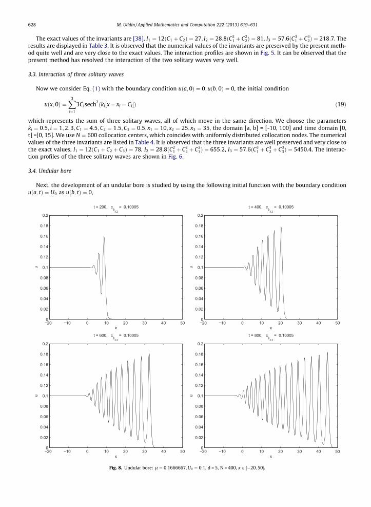
Fig. 8. Undular bore: l ¼ 0:1666667;U0 ¼ 0:1, d = 5, N = 400, x 2 ½�20;50�.

−40 −30 −20 −10 0 10 20 30 40−4

−3

−2

−1

0

1

2

3

4t = 0, cMQ = 0.06

x

u

−40 −30 −20 −10 0 10 20 30 40−4

−3

−2

−1

0

1

2

3

4t = 15, cMQ = 0.06

x

u

−40 −30 −20 −10 0 10 20 30 40−4

−3

−2

−1

0

1

2

3

4t = 50, cMQ = 0.06

x

u

−40 −30 −20 −10 0 10 20 30 40−4

−3

−2

−1

0

1

2

3

4t = 100, cMQ = 0.06

x

u

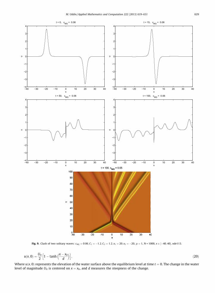
Fig. 9. Clash of two solitary waves: cMQ ¼ 0:06;C1 ¼ �1:2;C2 ¼ 1:2; x1 ¼ 20; x2 ¼ �20, l ¼ 1, N = 1000, x 2 ½�40;40�, ode113.


uðx;0Þ ¼ U0

21� tanh

x� x0

d

� �h i; ð20Þ

Where uðx;0Þ represents the elevation of the water surface above the equilibrium level at time t ¼ 0. The change in the waterlevel of magnitude U0 is centered on x ¼ x0, and d measures the steepness of the change.


We chose the parameters U0 ¼ 0:1;l ¼ 1; d ¼ 2 and x0 ¼ 0, and solved this problem on the domain [a, b] = [-20, 50] fortime up to t ¼ 800 with N ¼ 400 uniformly distributed nodes in the x domain. The solution profiles are shown in Fig. 7, andagreed with [45].

Next we chose another set of parameters U0 ¼ 0:1 d ¼ 5, l ¼ 0:1666667 and x0 ¼ 0, and solved this problem on the do-main [a, b] = [-20, 50] for time up to t ¼ 800 and with N ¼ 400 uniformly distributed nodes in the x domain. The solutionprofiles are shown in Fig. 8, which agree well with [14].

3.5. Soliton collision

Finally, we consider two solitary waves of the form

uðx;0Þ ¼ 3C1sech2ð0:5½x� x1 � C1�Þ þ 3C2sech2ð0:5½x� x2 � C2�Þ ð21Þ

The solitary waves are of exactly the same form but have different signs so they move toward each other. When they meet,they form a singularity which emits trains of smaller waves to both sides, while the singularity gradually vanishes over time,see Fig. 9. This example agrees with [45]. For this computation we chose the domain ½a; b� ¼ ½�40;40� and the parametersC1 ¼ �1:2;C2 ¼ 1:2; x1 ¼ 20; x2 ¼ �20;l ¼ 1, N ¼ 1000.

4. Concluding remarks

In this work, the RBF-PS scheme has been used to obtain numerical solutions of the equal width equation. We examinedthe motion of a solitary wave, the interaction of two and three solitary waves and the development of undular bore, and col-lision of two solitary waves. To show how good and accurate the present numerical scheme is, we computed the error normsand invariants of the model and compared the results of the present method with the available methods in the literature. TheRBF-PS method has been found to be very accurate. The scheme is fast and accurate enough to allow a thorough study of thedynamic behavior of solitary waves.

Acknowledgements

The author is thankful to the reviewers for their constructive and valuable comments.

References

[1] S.N. Atluri, S. Shen, The Meshless Method, Tech Science Press, Forsyth, 2002.[2] A.H.A. Ali, Spectral method for solving the equal width equation based on Chebyshev polynomials, Nonlinear Dyn. 51 (2008) 59–70.[3] B.G. Archilla, A spectral method for the equal width equation, J. Comput. Phys. 125 (1996) 395–402.[4] S.N. Atluri, T.L. Zhu, A new meshless local Petrov–Galerkin (MLPG) approach in computational mechanics, Comput. Mech. 22 (1998) 117–127.[5] Belytschko, T., Y. Krongauz, D.J. Orgam, M. Fleming, P. Krysl, Meshless methods: An overview and recent developments, Comput. Meth. Appl. Mech.

Eng., special issue, 139 (1996) 3–47.[6] M.D. Buhmann, Radial Basis Functions: Theory and Implementations, Cambridge University Press, 2003.[7] C.S. Chen, M. Ganesh, M.A. Golberg, A.H.D. Cheng, Multilevel compact radial basis functions based computational scheme for some elliptic problems,

Comput. Math. Appl. 43 (2002) 359–378.[8] I. Dag, B. Saka, A cubic B-spline collocation method for the EW equation, Math. Comput. Appl. 90 (2004) 381–392.[9] I. Dag�, Y. Dereli, Numerical solution of RLW equation using radial basis functions, Int. J. Comp. Math. 87 (2010) 63–76.

[10] M. Dehghan, A. Shokri, A numerical method for KdV equation using collocation and radial basis functions, Nonlinear Dyn. 50 (2007) 111–120.[11] J.R. Dormand, P.J. Prince, A family of embedded Runge–Kutta formulae, J. Comput. Appl. Math. 6 (1980) 19–26.[12] Y. Dereli, R. Schaback, The meshless kernel-based method of lines for solving the equal width equation, Appl. Math. Comput. 219 (2013) 5224–5232.[13] A. Dogan, Application of the Galerkin’s method to equal width wave equation, Appl. Math. Comput. 160 (2005) 65–76.[14] A. Esen, A numerical solution of the equal width wave equation by a lumped Galerkin method, Appl. Math. Comput. 168 (2005) 270–282.[15] A. Esen, S. Kutluay, A linearized implicit finite-difference method for solving the equal width wave equation, Int. J. Comp. Math. 83 (2006) 319–330.[16] E.G. Fasshauer, Meshfree Approximation Methods with MATLAB, Collection Interdisciplinary Mathematical Sciences, vol. 6, World Scientific Publishers,

Singapore, 2007.[17] E.G. Fasshauer, RBF collocation method and pseudospectral methods, Illinois Institute of Technology, 2005 (Preprint).[18] G.E. Fasshauer, J.G. Zhang, On choosing optimal shape parameters for RBF approximation, Numer. Algorithms 45 (2007) 345–368.[19] A.M.A. Ferreira, G.E. Fasshauer, Computation of natural frequencies of shear deformable beams and plates by an RBF-PS method, Comput. Meth. Appl.

Mech. Eng. 196 (2006) 134–146.[20] A.M.A. Ferreira, G.E. Fasshauer, Analysis of natural frequencies of composite plates by an RBF-PS method, Compos. Struct. 79 (2007) 202–210.[21] J. Franke, Scattered data interpolation: tests of some methods, Math. Comput. 48 (1982) 181–200.[22] L.R.T. Gardner, G.A. Gardner, F.A. Ayoub, M.K. Amein, Simulations of the EW undular bore, Commun. Numer. Meth. Eng. 13 (1997) 583–592.[23] L.R.T. Gardner, G.A. Gardner, Solitary waves of the equal width wave equation, J. Comput. Phys. 101 (1992) 218–223.[24] B. Garcia Archilla, A spectral method for the equal width equation, J. Comput. Phys. 125 (1996) 395–402.[25] R.L. Hardy, Least square prediction, Photogrammetric Eng. Remote Sens. 43 (1977) 475–492.[26] Y.C. Hon, X.Z. Mao, An efficient numerical scheme for Burger’s equations, Appl. Math. Comput. 95 (1998) 37–50.[27] Y.C. Hon, R. Schaback, X. Zhou, An adaptive greedy algorithm for solving large RBF collocation problems, Numer. Algorithms 32 (2003) 13–25.[28] G.E. Fasshauer, A.Q. M. Khaliq, D.A. Voss, Using meshfree approximation for multi-asset American options, J. Chinese Inst. Engrs. 27 (2004) 563–571.[29] E.J. Kansa, Multiquadrics – a scattered data approximations cheme with application to computational fluid dynamics, part I. Surface approximations

and partial derivative estimates, Comput. Math. Appl. 19 (1990) 127–415.[30] E.J. Kansa, Multiquadrics – a scattered data approximations cheme with applications to computational fluid dynamics, part II. Solutions to parabolic,

hyperbolic and elliptic partial differential equations, Comput. Math. Appl. 19 (1990) 147–161.

http://refhub.elsevier.com/S0096-3003(13)00781-9/h0005






































[31] E.J. Kansa, Y.C. Hon, Circumventing the ill-conditioning problem with multiquadric radial basis functions: applications to elliptic partial differentialequations, Comput. Math. Appl. 39 (2000) 123–137.

[32] A.K. Khalifa, K.R. Raslan, Finite difference methods for the equal width wave equation, J. Egypt. Math. Soc. 7 (1999) 239–249.[33] G.R. Liu, Meshfree methods: moving beyond the finite element method, CRC Press, Boca Raton, 2003.[34] L. Ling, R. Schaback, Stable and convergent unsymmetric meshless collocation methods, SIAM J. Numer. Anal. 46 (2008). pp. 1097–1015.[35] N. Mai-Duy, T. Tran-Cong, Numerical solution of Navier–Stokes equations using multiquadric radial basis function networks, Neural Networks 14

(2001) 185–199.[36] N. Mai-Duy, T. Tran-Cong, Mesh-free radial basis function network methods with domain decomposition for approximation of functions and numerical

solution of Poisson’s equation, Eng. Anal. Bound. Elem. 26 (2002) 133–156.[37] P.J. Morrison, J.D. Meiss, J.R. Carey, Scattering of RLW solitary waves, Physica D. 11 (1981) 324–336.[38] K.R. Raslan, A computational method for the equal width equation, Int. J. Comput. Math. 81 (2004) 63–72.[39] K.R. Raslan, Collocation method using quartic B-spline for the equal width equation, Appl. Math. Comput. 168 (2005) 795–805.[40] C.M.C. Roque et al, Dynamic analysis of functionally graded plates and shells by radial basis functions, Mech. Adv. Mater. Struct. 17 (2010) 636–652.[41] C.M.C. Roque et al, Transient analysis of composite and sandwich plates by radial basis functions, J. Sand Struct. Mater. 13 (2011) 681–704.[42] B. Saka, A finite element method for equal width equation, Appl. Math. Comput. 175 (2006) 730–747.[43] B. Saka, I. Dag, Y. Dereli, A. Korkmaz (Three different methods for numerical solution of the EW equation), Eng. Anal. Bound. Elem. 32 (2008) 556–566.[44] R. Schaback, Convergence of unsymmetric kernel-based meshless collocation methods, SIAM J. Numer. Anal. 45 (2007) 333–352.[45] R. Schaback, Unsymmetric meshless method for operator equations, Numer. Math. 114 (2010). pp. 929–651.[46] R. Schaback, Error estimates and condition numbers for radial basis function interpolation, Adva. Comput. Math. 3 (1995) 389–396.[47] L.F. Shampine, M.K. Gordon, Computer Solution of Ordinary Differential Equations: the Initial Value Problem, W.H. Freeman, SanFrancisco, 1975.[48] C. Shu, H. Ding, S. Yeo, Local radial basis function-based differential quadrature method and its application to solve two-dimensional incompressible

Navier–Stokes equations, Comput. Method. Appl. Mech. Eng. 192 (2003) 941–954.[49] L.N. Trefethen, Spectral Methods in MATLAB, SIAM, Philadelphia, 2000.[50] M. Uddin et al, A mesh-free numerical method for solution of the family of Kuramoto–Sivashinsky equations, Appl. Math. Comput. 212 (2009) 458–

469.[51] M. Uddin et al, Numerical solution of complex modified Kortewege–de Vries equation by mesh-free collocation method, Comput. Math. Appl. 58

(2009) 566–578.[52] M. Uddin, S. Haq, RBFs approximation method for time fractional partial differential equations, Commun. Nonlinear Sci. Numer. Simul. 16 (11) (2011)

4208–4214.[53] M. Uddin, On the selection of a good value of shape parameter in solving time-dependent partial differential equations using RBF approximation

method, Appl. Math. Model. http://dx.doi.org/10.1016/j.apm.2013.05.060.[54] M. Uddin, S. Ali, RBF-PS method and fourier pseudospectral method for solving stiff nonlinear partial differential equations, Math. Sci. Lett. 2 (1) (2012)

55–61.[55] M. Uddin, R.J. Ali, RBF-PS scheme for the numerical solution of the complex modified Korteweg–de Vries equation, Appl. Math. Inf. Sci. Lett. 1 (1) (2012)

917.[56] S.I. Zaki, A least-squares finite element scheme for the EW equation, Comput. Meth. Appl. Mech. Eng. 189 (2000) 587–594.[57] S.I. Zaki, Solitary waves induced by the boundary forced EW equation, Comput. Meth. Appl. Mech. Eng. 190 (2001) 4881–4887.

































http://dx.doi.org/10.1016/j.apm.2013.05.060







Documents

RBF-PS scheme for solving the equal width equation