Zekuang Tan

January, 2018

Working Paper No. 17-044

RBC LiONS™ S&P 500 Buffered Protection Securities

(USD) Series 4 Analysis

Option Pricing Analysis, Issuing Company Risk-

hedging Analysis, and Recommended Investment

Strategy

RBC LiONS™ S&P 500 Buffered Protection Securities USD Series 4 Analysis

Option Pricing Analysis, Issuing Company Risk-hedging Analysis, and Recommended Investment Strategy

5th Solution Fund

Zekuang Tan (Tyson)

Abstract

This paper will compute the value of the RBC financial derivative-RBC LiONS™ S&P 5 Buffered Protection Securities (USD), Series 4 by utilizing the Black-Scholes Option Pricing

Model. In order conduct a thorough analysis of the securities, the paper will compare the

model value with the actual price at which the security was issued and the price at which it

was traded. This model will help establish a recommended strategy for the issuing company

to hedge the liability incurred by the security issued, and provide a possible hedging

strategy for the investors.

Introduction

The objective of the paper to compute the value of the RBC financial derivative-RBC LiONS™ S&P 500 Buffered Protection Securities (USD), Series 4 by using the Black-Scholes under

Option Pricing Model. Further we analyze the security described in the product offering

from the viewpoint of the issuing company and from the viewpoint of an investor

considering whether or not to buy them. In this scenario Royal Bank of Canada (RBC)

offered up to $ , , US dollars of RBC LiONS™ S&P 5 Buffered Protection Securities (Macroption, 2013). Moreover, Series 4 is for investors that need to reach a large segment of

the United States equity market and therefore this product is necessary for them

(Macroption, 2013). Furthermore, principal of securities can protect when up against a

decline of up to 30% when the price performance and maximum return is 41% (Macroption,

2013). This is due to the fact that the payment, which is paid at maturity on these specific

securities, is based on the price performance of S&P 500® Index subject to a buffer of 30%

and a cap of 41% (Macroption, 2013). If there is a negative performance that exceeds 30%,

the amount of the principal could be lost in the maturity (Macroption, 2013).

Black Schole Model

In 1973, the Chicago Board of Options Exchange began trading options in exchanges,

although previously financial institutions in had regularly traded options over the counter

markets (Macroption, 2013). During the same year, Black and Scholes (1973), and Merton

(1973), published their seminal papers on the theory of option pricing (Macroption, 2013).

The time since the seminal papers have caused the growth of the derivative securities field

to become incredible. In 1997, Scholes and Merton received a Nobel Prize within the

Economics discipline in order to recognize their contributions to option valuations

(Macroption, 2013). During the ceremony, Black was unable to receive his award because

he had passed away but he was known as someone that left this world a little better than he

found it. Overall, the Black-Scholes model is able to eliminate all market risks by simply

continuously adjusting proportions of stocks and options in a portfolio, as this will allow an

investor to craft a riskless hedge portfolio (Macroption, 2013). This portfolio would be

dependent on the assumptions of continuous trading and sample paths of the asset price

(Macroption, 2013). Further, all portfolios that exhibit a zero market risk must have an

expected rate of return equal to the risk-free interest rate within an efficient market that

showcases no riskless arbitrage opportunities. This is an approach that leads to a

differential equation that is known as the heat equation . The solution in this scenario is

the Black-Scholes formula for pricing European options on non-dividend paying stocks

shown below (Macroption, 2013). Overall, in a study six different stocks were compared to

the real market and the Black Scholes model and the result was striking similarities

(Macbeth, J. D., & Merville, L. J., 1979). Moreover, this model’s predicted prices are on

average less (greater) than market prices for in the money (out of the money) options

(Macbeth, J. D., & Merville, L. J., 1979). According to the research done by Black and Scholes

by thorough empirical tests actual prices at which options are bought and sold deviate in

certain systematic ways from the values predicted by the formula (Black, F., & Scholes, M.,

1979).

As stated above, there are several assumptions that must be acknowledged in order to

effectively utilize the model. The first assumption is that the price of the instrument is a

geometric Brownian motion, which embodies constant drift and volatility (Macroption,

2013). Next, it is possible to short sell the underlying stock and there are absolutely no

riskless arbitrage opportunities even though it may seem as this is the truth. Following this,

it is vital to understand trading in the stock is continuous, there are no transaction costs,

and every security is perfectly divisible. Finally, the risk-free interest rate is constant and

the same for every maturity date (Macroption, 2013). Finally, Black and Scholes did

another empirical study alongside Michael C. Jensen from Harvard Business School

showcasing the power of this model and vital assumptions. Specifically, as shown above

they relate to portfolios mean and variance, transaction costs, homogeneous views, and

riskless rate (Black , F., Jensen, M., & Scholes, M., 1972).

SPX Index Data Collection

In order to value a derivative, it is vital to estimate the volatility of its underlying asset. This

will require obtaining data on the weekly return on SPX Index for a period of about 6

months to 1 year preceding the date on which the security is priced. One is able to collect

this date (from 2011,11,22 to 2016,11,22) by accessing the Bloomberg terminals and

importing the data to Excel.

Cash Flows of Security

From an investor’s point of view, this security has an initial cash flow, which is its Principal

Amount, -$100 per security. On the mature date, the cash inflow has four possible outcomes

dependent on the index market return: $141(Percentage Change>41%), $100+$100*percentage

change (41%>Percentage Change>0), $100 (percentage change<-30%), or $100*percentage

change (percentage change<30%) per security.

T0 T

St = S0*∆

Index S0 ∆<0.7 ∆=0.7~1 ∆=0.7~1.41 ∆>1.41

Cash -100 100*(∆+0.3) 100 100*∆ 141

Fair Market Value of the Security at the Time of Issue and on the Present

Prior to addressing the fair market value it is important to outline the assumptions used during the

calculations. The primary assumption is that the interest rate is risk free. Rf of the issuing day is

set to be 5-year US Treasury bill rate of that day because the product has a 5-year investment

horizon; and Rf of today is set to be 1-year US treasury bill rate of November 22, 2016 because

there is 1 year from now to maturity. The second assumption is related to the dividend yield.

Specifically, the annual dividend yield of the issuing day is set to be 2.14% constant (retrieved

from pricing supplements); that of today is set to be 2.05% (retrieved from SP500). The third

assumption is that the future stock price and return is normally distributed. Finally, the last

assumption is related to implied volatility. Specifically, it is computed using the return of one

year preceding the calculation day.

0

20

40

60

80

100

120

140

160

-150% -100% -50% 0% 50% 100% 150%

Payoff diagram

The following is a thorough description of the calculations. The initial index level is $1417.27

(the price of the fourth exchanging day preceding the issuing day). Therefore, the payoff of one

share of index can be represented with a 41% cap equals to $1998.34 and a 30% buffer at the

level $992.08. And then we replicate the securities by constructing a portfolio using a

combination of put and a bond.

The replicated portfolio consists of short position of two put options at strike price of $1998.34

and $992.08, respectively, and long position of a put at $1417.27, and selling a bond with its

future value equals to $581.08.

The portfolio pricing was calculated to be $63.98 for issuing day, and $534.05 for today, for each

share of the underlying asset. As one security represents $100, the fair values per security for the

issuing day and present day would be $104.52 and $137.68, respectively.

Pricing issuing day

σ 14.74%

T 5

div 2.14%

5 yr treasury rate on nov 9 2012 0.65%

Replication

K d1 N-d1 d2 N-d2 Put

Short put cap 1998.337 -1.103 0.865 -1.433 0.924 685.950

Short put buffer 992.082 1.021 0.154 0.691 0.245 39.342

Long put initial 1417.260 -0.061 0.524 -0.391 0.652 226.780

FV PV

Lend 581.077 562.495

PV of portfolio $ (63.98)

PV 1 unit of security $ (4.51)

PV pricing $ 104.51

Pricing today

σ 14.01%

T 0.976190476

Div 2.05%

1 yr treasury rate on nov 22 2016 0.78%

S today 2202.94 (246 days to maturity)

Replication

K d1 N-d1 d2 N-d2 Put

Short put cap 1998.337 0.684 0.247 0.546 0.293 47.095

Short put buffer 992.082 5.744 0.000 5.606 0.000 0.000

Long put initial 1417.260 3.167 0.001 3.028 0.001 0.065

FV PV

Lend 581.077 581.077

PV of portfolio $ (534.05)

PV 1 unit of security $ (37.68)

PV pricing $ 137.68

Comparison of Model to Actual Price During Issue Date and Present

Issue day Today

BS model 104.5146 137.6816

Actual price 100 133.54

Difference 4.514595 4.14161

When we compare the model value with the actual price, the model prices are slightly higher both

in 2012 and 2016 (4.5 and 4.1 respectively). For the issue price, the difference can be caused by

two possibilities including the bank may not use Black Scholes model for option pricing, or that

the inputs are different.

Binomial model and Monte Carlo simulation also can be appropriate choices of valuation. And

also, sometimes banks make small tweaks to the model because they are fully aware of the

limitation of Black Schole method. Similar to return, it is assumed as normally distributed.

However, in reality, the normal distribution is very unlikely to happen. As for the inputs, there

have been a few simple assumptions included (see previous section) for calculation purposes,

which could be inaccurate.

Also, Black Scholes model assumes a constant risk free rate, and normal distribution for stock

price, which are not realistic given that the market is very dynamic and complex (NYU, 2013).

Therefore, when pricing the options at the bank, individuals notice these problems and slightly

change the valuation.

The difference from today’s price is because the model price is not the same as market price. The

market price is “determined in the market by the interaction of supply and demand for the

particular option.” In comparison, the model price is created based on different assumptions, such

as constant interest rate. However, it ignores the market interactions, which results in difference

from the current market price.

Recommended Strategy to Hedge the Liability

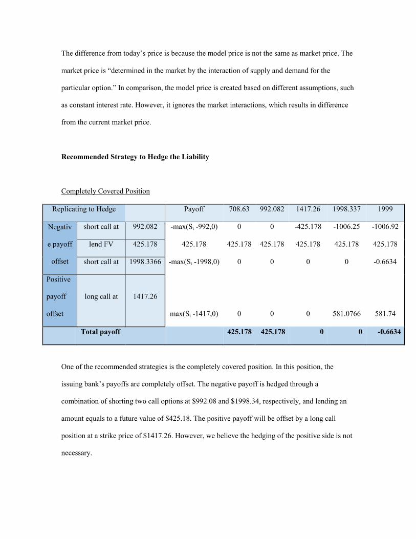
Completely Covered Position

Replicating to Hedge

Payoff 708.63 992.082 1417.26 1998.337 1999

Negativ

e payoff

offset

short call at 992.082 -max(St -992,0) 0 0 -425.178 -1006.25 -1006.92

lend FV 425.178 425.178 425.178 425.178 425.178 425.178 425.178

short call at 1998.3366 -max(St -1998,0) 0 0 0 0 -0.6634

Positive

payoff

offset

long call at 1417.26

max(St -1417,0) 0 0 0 581.0766 581.74

Total payoff 425.178 425.178 0 0 -0.6634

One of the recommended strategies is the completely covered position. In this position, the

issuing bank’s payoffs are completely offset. The negative payoff is hedged through a

combination of shorting two call options at $992.08 and $1998.34, respectively, and lending an

amount equals to a future value of $425.18. The positive payoff will be offset by a long call

position at a strike price of $1417.26. However, we believe the hedging of the positive side is not

necessary.

Through the completely hedged position, regardless of the future stock price, the payoff is going

to be consistent for the issuing bank.

Delta Dynamic Hedging

Replicating Security

Payoff 708.63 992.082 1417.26 1998.337 200000

Long call at 992.082 max(St -992,0) 0 0 425.178 1006.255 199007.9

Borrow FV -425.178 -425.178 -425.178 -425.178 -425.178 -425.178 -425.178

Long call at 1998.3366 max(St -1998,0) 0 0 0 0 198001.7

Short call at 1417.26 -max(St -1417,0) 0 0 0 -581.077 -198583

Total payoff -425.178 -425.178 0.00 0 198001.7

Delta Dynamic Hedging is another effective strategy. Dynamic hedging through constructing a

delta neutral portfolio is another way for the issuing bank to hedge against the volatility of the

index. This strategy is known as an options strategy that is able to reduce, or hedge, the risk with

price movement in the underlying asset, which is performed by offsetting long and short positions

(NYU, 2013). For example, a long call position may be delta hedged by shorting the

underlying stock. This strategy is based on the change in premium, or price of option,

caused by a change in the price of the underlying security (NYU, 2013).

From the RBC’s perspective, the security payoff was replicated with two long call options at

992.08, and 1998.34 respectively, a short call at 1417.26, as well as a bond purchasing (money

borrowing) with a future value equals to 425.18. To illustrate the strategy, it is assumed the index

follows a Geometric Brownian Motion and simulated a complete path for the index over its 5

years life span.

As delta of an option being the rate of change of the option price with respect to the price of the

underlying asset, assuming no arbitrage, it means that the delta for the security should be

consistent with that of its replicated portfolio.

Therefore, we obtained the security’s delta value D through computing the delta value for its

replicated portfolio. And then short D shares of index to achieve delta neutral.

The number of shares will be adjusted over time to ensure zero sensitivity to stock price change.

Interesting Features in the Issued Security

The security is suitable for the investors who prepared to hold the security to maturity over the 5-

year investment horizon and do not expect to regular payments. The minimum investment is 50

securities or US $5000. The principal amount per security is US$100, so is the minimum

increment of the investment.

The initial index level is the closing index level on the fourth Exchange Day immediately

preceding the issue date of the securities. The final index level is the closing index level on the

third Exchange Day immediately preceding the maturity date of the securities.

Factors that Influence the Pricing on the Securities

Tax Treatment of Capital Gain and Losses

The taxable capital gain income equals to one-half of any capital gain realized, whereas one-half

of any capital loss incurred will constitute an allowable capital loss that is deductible against

taxable capital gains of the Resident Holder. Also, noting the security is eligible for RRSPs,

RRIFs, RESPs, RDSPs, DPSPs and TFSA, in which case the Resident Holder can arrange the tax

expenses of the year accordingly.

Risk Factors

The first risk is credit risk. Since structured notes are an IOU from the issuer, the investors bear

the risk that the investment bank forfeits on the debt. A structured note adds a layer of credit risk

on top of the market risk. Market risks are vital to address in this scenario. The partially protected

security has large exposure to the large-cap segment of the US equity market. The amount being

repaid on the maturity date is not fixed, which means the return could be positive or negative.

Despite there are 30% buffers on the price drop, the principal amount of the security is still fully

exposed, and the investor could lose a significant amount on the investment. Finally, the last risk

to consider is liquidity risk. According to the prospect, we notice that the securities will not be

listed on any stock exchange. It may be resold using the FundSERV network, however there is no

assurance that a secondary market will develop or be sustained. In case of resale, the price is

determined at the time of sale by the Calculation Agent. The price is likely to be lower than the

Principal Amount and it will be subject to specified early trading charges, depending on the

timing. Noted the bank may have the right to redeem or “call” the securities prior to their maturity,

which terminate the investor’s entitlement to any appreciation in index level or any regular

payment of interest or principal.

Possible Hedging Strategy for the Investors

Investor is likely to hedge the situation when the price drops below 30% of the index. There are

two methods to address this. The first method is using the completely covered position, so that the

bank’s payoffs are completely offset. The negative payoff are hedged through a combination of

shorting two call options at $992.08 and $1998.34, respectively, and lending an amount equals to

a future value of $425.18. The second method is hedging the negative payoff using short put

position with a strike price of $992.08. The credit risk of the security coming from the issuing

bank RBC, although we believe it is extremely unlikely, in the case of default; investor could

hedge it by utilizing credit insurance or default swap.

Conclusion

In conclusion, the RBC security is a sound investment that given the thorough analysis described

above. The Black Scholes model has showcased similar numbers with little variances allowing

one to understand the power of this model. There may be other models that would be able to get

closer to the actual amount; however, this is difficult to overcome without the assumptions that

have been outlined. Although there are various risk factors associated with this investment it is a

rare occurrence and therefore the suggestion is to take part in this security. Moreover, in order to

ensure success it is necessary to follow the various recommendations outlined above as well as

understanding the precautions outlined. Overall, the RBC investment has showcased the

probability of a positive investment.

References

Black , F., Jensen, M., & Scholes, M. (1972). The Capital Asset Pricing Model: Some Empirical

Tests. The Capital Asset Pricing Model: Some Empirical Tests.

Black, F., & Scholes, M. (1979). The Pricing of Options and Corporate Liabilities . Journal of

Political Economy .

Macbeth, J. D., & Merville, L. J. (1979). An Empirical Examination of the Black-Scholes Call

Option Pricing Model. The Journal of Finance,34(5), 1173-1186. doi:10.1111/j.1540-

6261.1979.tb00063.x

Macroption. (2013). Strike vs. Market Price vs. Underlying Price. Retrieved January 03, 2018,

from http://www.macroption.com/option-strike-market-underlying-price/

NYU. (2013). Some Drawbacks of Black Scholes. Retrieved from

http://people.stern.nyu.edu/churvich/Forecasting/Handouts/Scholes.pdf