Embed Size (px)
Citation preview
R.B. Von Dreele, Advanced Photon Source
Argonne National Laboratory
Rietveld Refinement with GSAS
Recent Quote seen in Rietveld e-mail:
“Rietveld refinement is one of those few fields of intellectual endeavor wherein the more one does it, the less one understands.” (Sue Kesson)
Demonstration – refinement of fluroapatite
Stephens’ Law – “A Rietveld refinement is never perfected,
merely abandoned”
2
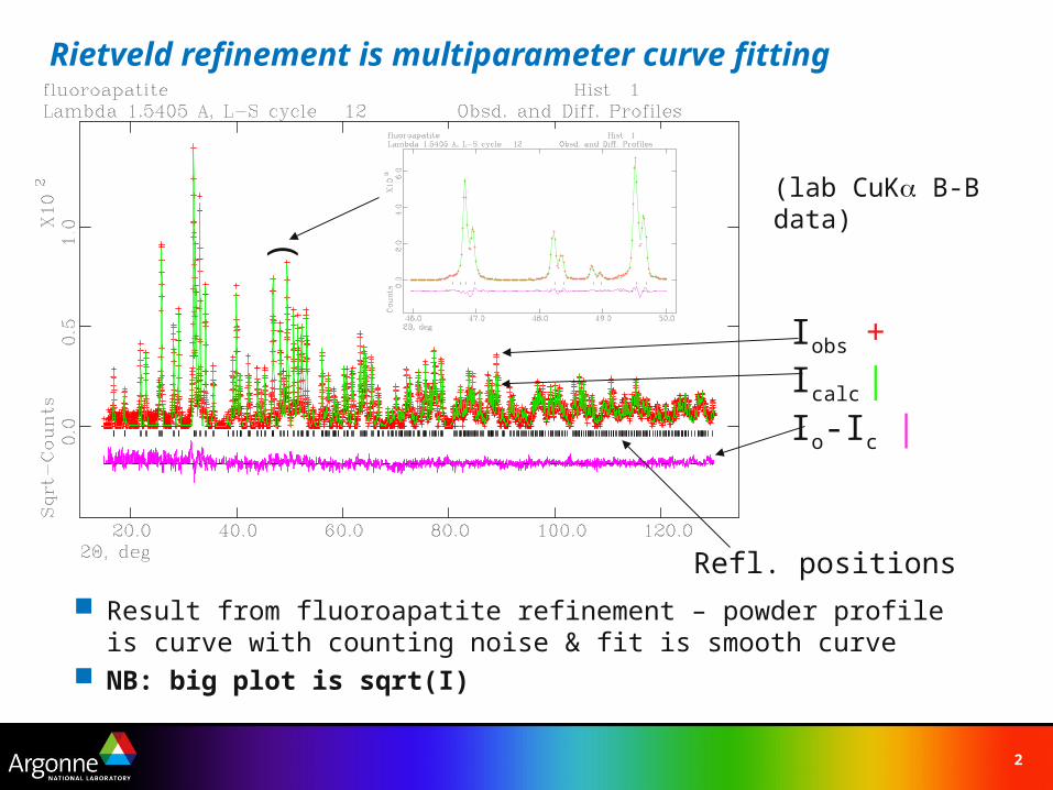
Result from fluoroapatite refinement – powder profile is curve with counting noise & fit is smooth curve
NB: big plot is sqrt(I)
Rietveld refinement is multiparameter curve fitting
Iobs +Icalc |Io-Ic |
)
Refl. positions
(lab CuK B-B data)
3
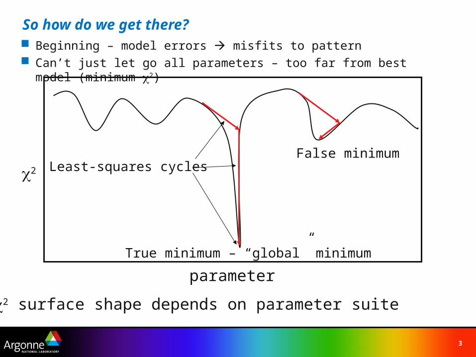
So how do we get there? Beginning – model errors misfits to pattern Can’t just let go all parameters – too far from best model (minimum 2)
2
parameter
False minimum
True minimum – “global” minimum
Least-squares cycles
2 surface shape depends on parameter suite
4
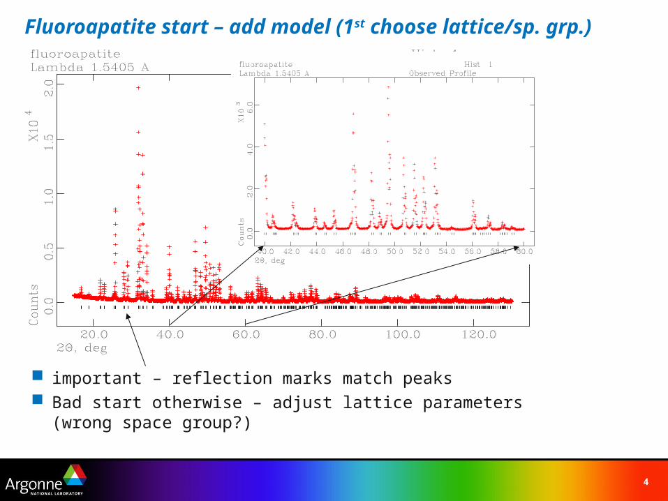
Fluoroapatite start – add model (1st choose lattice/sp. grp.)
important – reflection marks match peaks Bad start otherwise – adjust lattice parameters (wrong space group?)
5
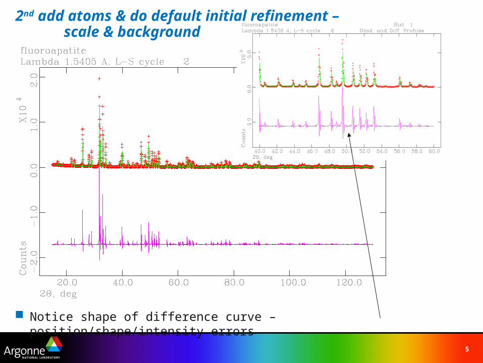
2nd add atoms & do default initial refinement – scale & background
Notice shape of difference curve – position/shape/intensity errors
6
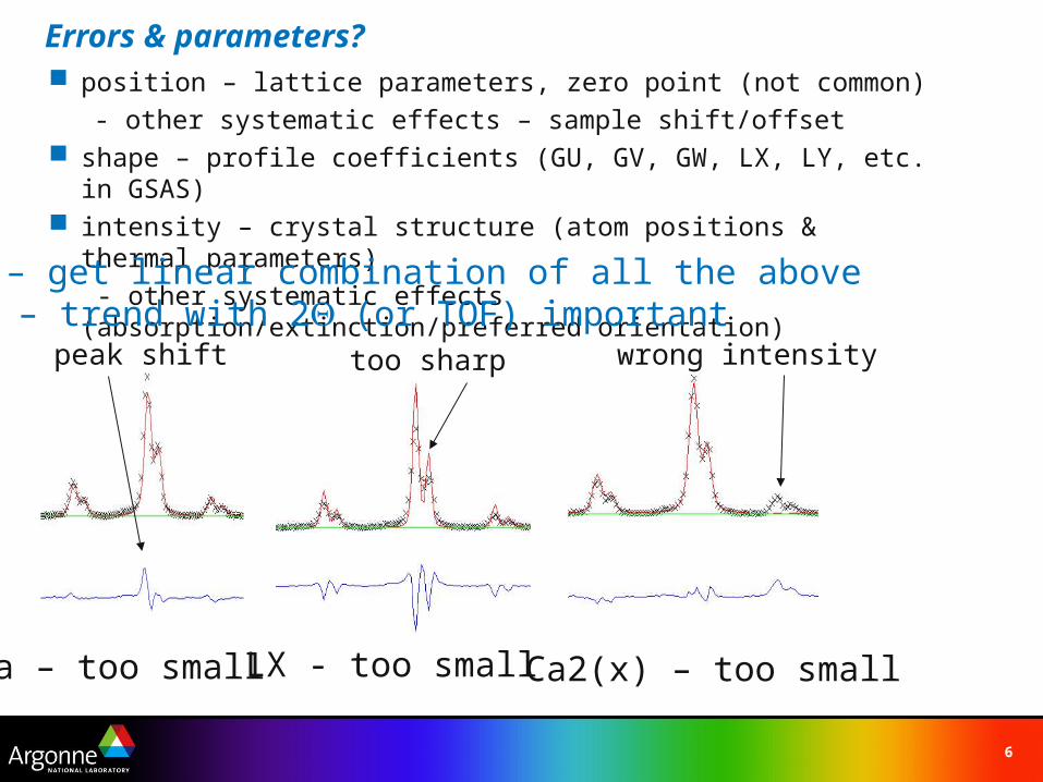
Errors & parameters? position – lattice parameters, zero point (not common)
- other systematic effects – sample shift/offset shape – profile coefficients (GU, GV, GW, LX, LY, etc. in GSAS) intensity – crystal structure (atom positions & thermal parameters)
- other systematic effects (absorption/extinction/preferred orientation)
NB – get linear combination of all the aboveNB2 – trend with 2(or TOF) important
a – too small LX - too small Ca2(x) – too small
too sharppeak shift wrong intensity
7
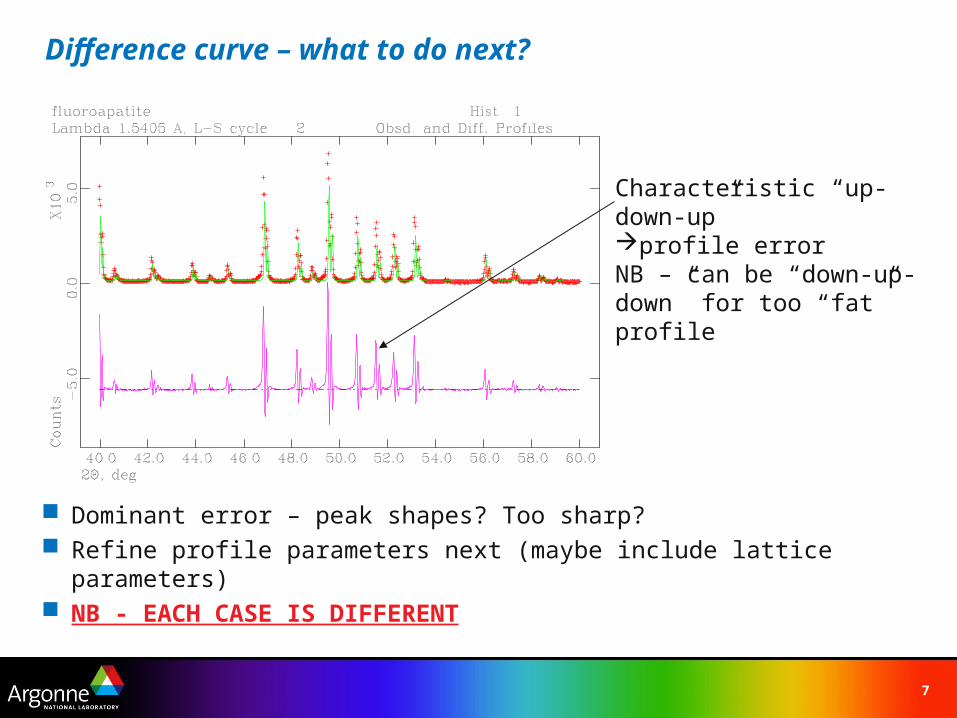
Difference curve – what to do next?
Dominant error – peak shapes? Too sharp? Refine profile parameters next (maybe include lattice parameters) NB - EACH CASE IS DIFFERENT
Characteristic “up-down-up”profile errorNB – can be “down-up-down” for too “fat” profile
8
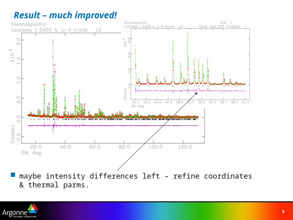
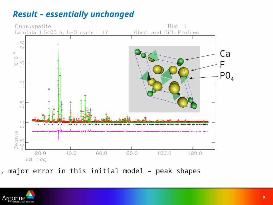
Result – much improved!
maybe intensity differences left – refine coordinates & thermal parms.
9
Result – essentially unchanged
Thus, major error in this initial model – peak shapes
CaFPO4
10
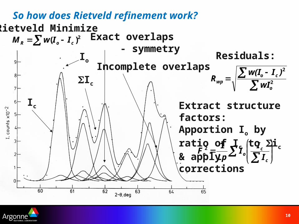
So how does Rietveld refinement work?
Exact overlaps - symmetry
Incomplete overlaps
c
coo I
II
LpF
12
Extract structure factors: Apportion Io by ratio of Ic to ic & apply corrections
Io
Ic
2
2
o
cowp wI
)Iw(IR
Residuals:
Rietveld Minimize 2)( coR IIwM
Ic
11
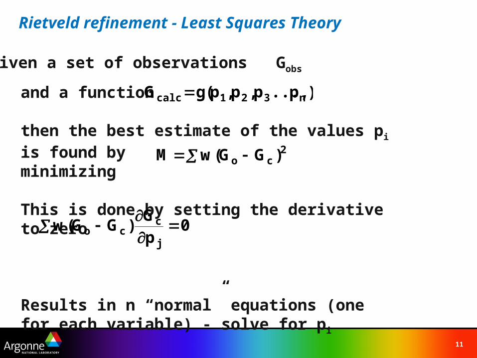
Rietveld refinement - Least Squares Theory
and a function
then the best estimate of the values pi is found by minimizing
This is done by setting the derivative to zero
Results in n “normal” equations (one for each variable) - solve for pi
)p...,p,p,p(gG n321calc
Given a set of observations Gobs
2co )GG(wM
0pG
)GG(wj
cco
12
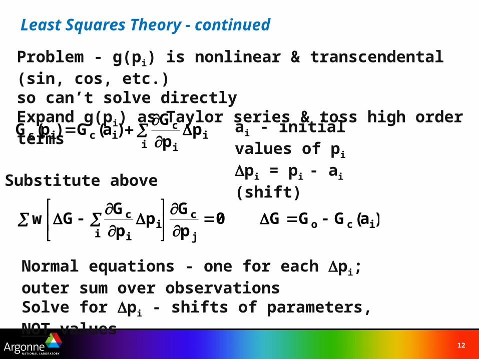
Least Squares Theory - continued
Problem - g(pi) is nonlinear & transcendental (sin, cos, etc.)so can’t solve directlyExpand g(pi) as Taylor series & toss high order terms
i
ii
cicic p
pG
)a(G)p(G
Substitute above
ai - initial values of pi
pi = pi - ai (shift)
)a(GGG0pG
ppG
Gw icoj
c
ii
i
c
Normal equations - one for each pi; outer sum over observationsSolve for pi - shifts of parameters, NOT values
13
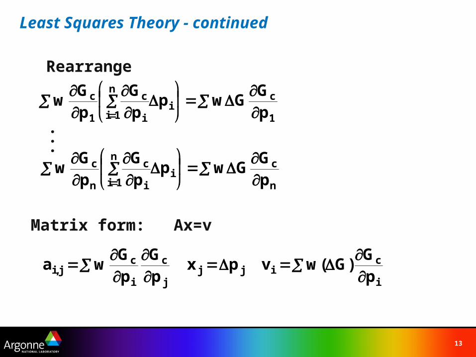
Least Squares Theory - continued
Rearrange
1
ci
n
1i i
c
1
c
pG
GwppG
pG
w
...
n
ci
n
1i i
c
n
c
pG
GwppG
pG
w
Matrix form: Ax=v
i
cijj
j
c
i
cj,i p
G)G(wvpx
pG
pG
wa
14
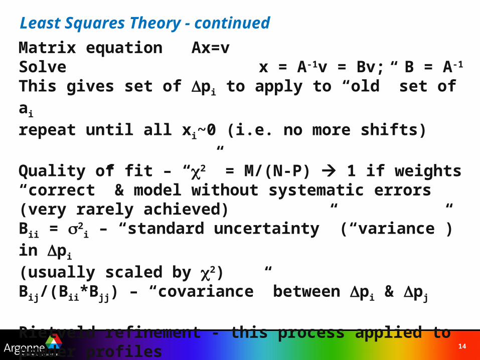
Least Squares Theory - continued
Matrix equation Ax=vSolve x = A-1v = Bv; B = A-1
This gives set of pi to apply to “old” set of ai
repeat until all xi~0 (i.e. no more shifts)
Quality of fit – “2” = M/(N-P) 1 if weights “correct” & model without systematic errors (very rarely achieved)Bii = 2
i – “standard uncertainty” (“variance”) in pi
(usually scaled by 2)Bij/(Bii*Bjj) – “covariance” between pi & pj
Rietveld refinement - this process applied to powder profilesGcalc - model function for the powder profile (Y elsewhere)
15
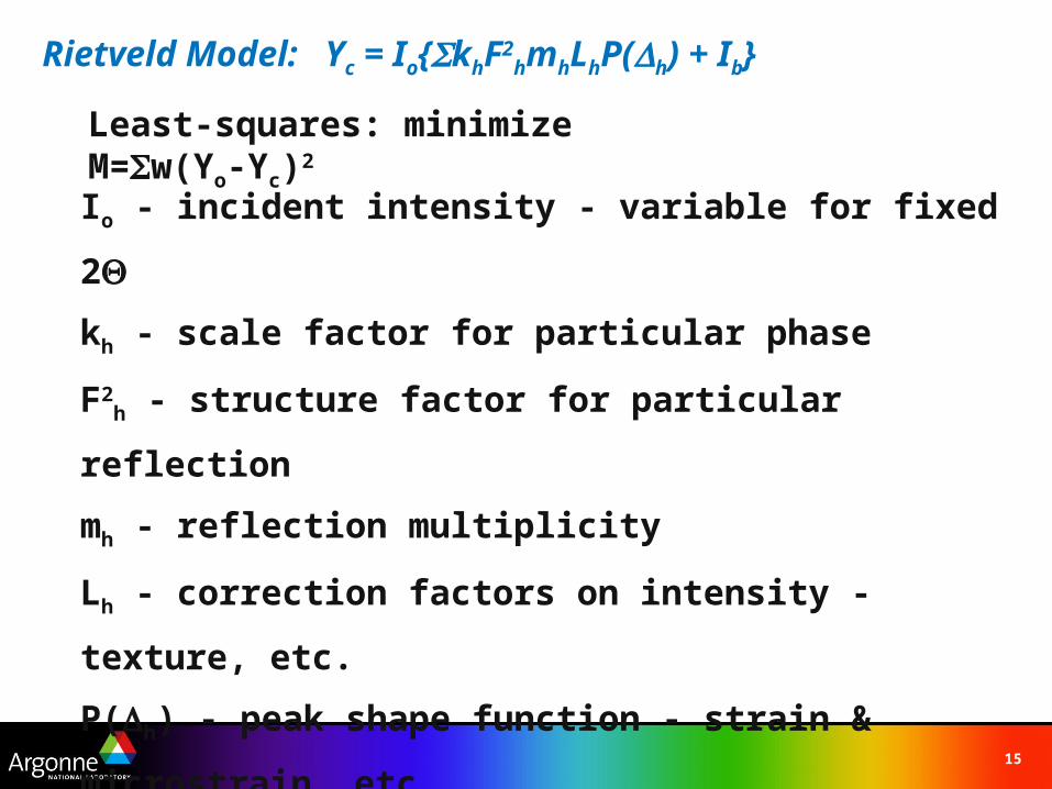
Rietveld Model: Yc = Io{khF2hmhLhP(h) + Ib}
Io - incident intensity - variable for fixed 2
kh - scale factor for particular phase
F2h - structure factor for particular reflection
mh - reflection multiplicity
Lh - correction factors on intensity - texture, etc.
P(h) - peak shape function - strain & microstrain, etc.
Ib - background contribution
Least-squares: minimize M=w(Yo-Yc)2
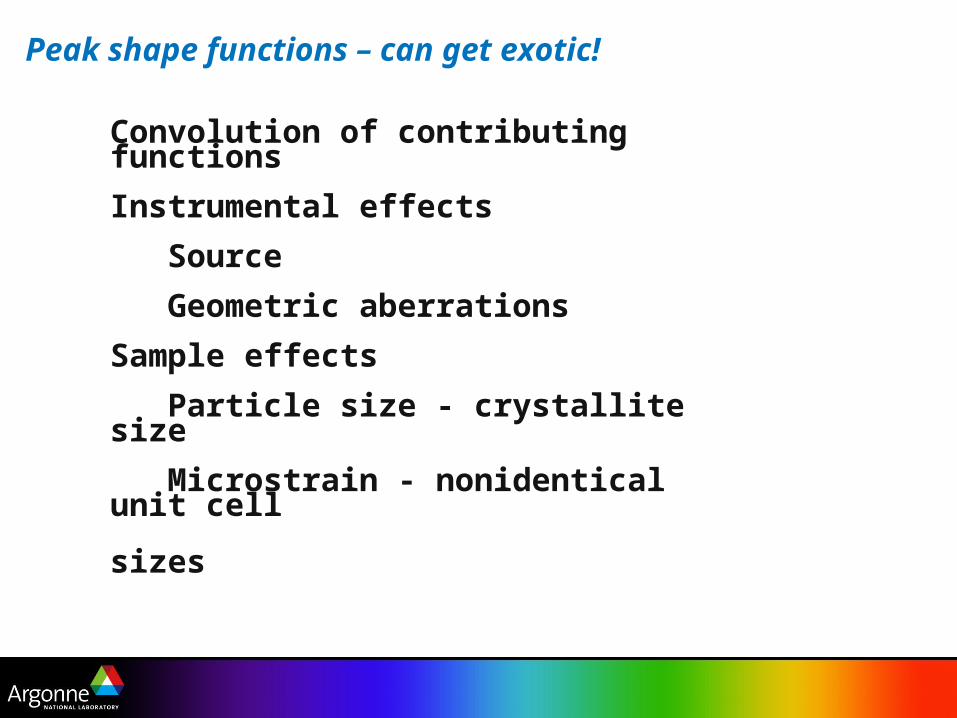
Convolution of contributing functions
Instrumental effects
Source
Geometric aberrations
Sample effects
Particle size - crystallite size
Microstrain - nonidentical unit cell sizes
Peak shape functions – can get exotic!
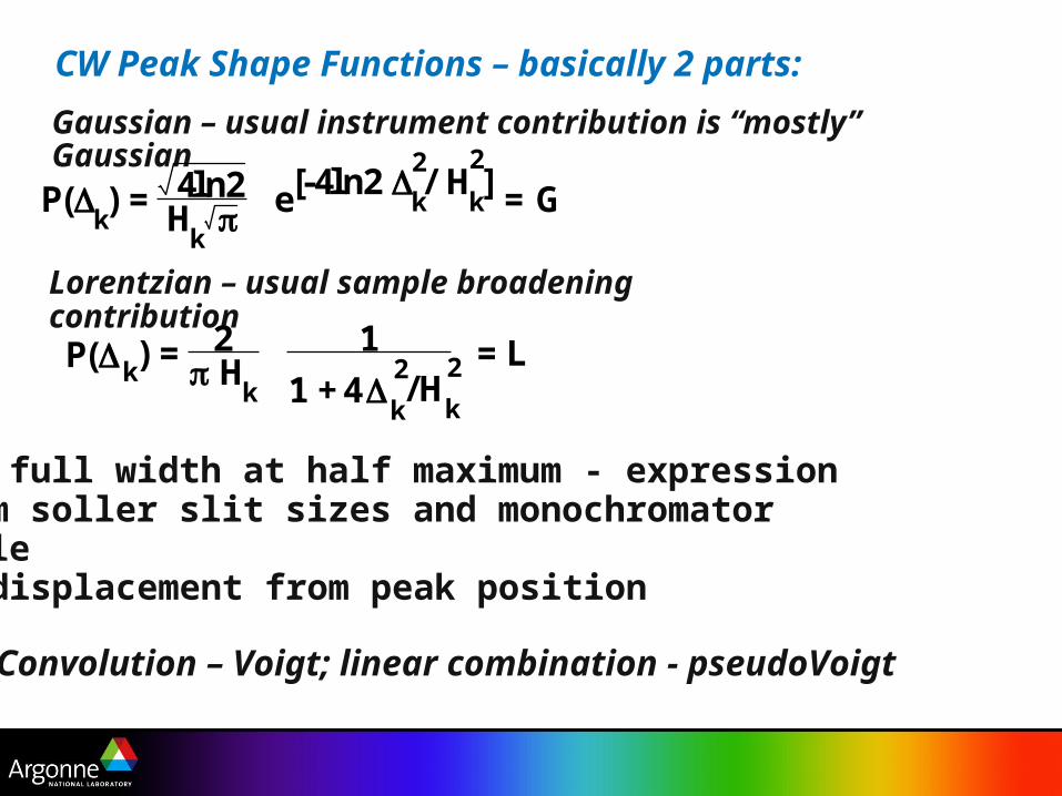
Gaussian – usual instrument contribution is “mostly” Gaussian
H - full width at half maximum - expressionfrom soller slit sizes and monochromatorangle- displacement from peak position
P(k) = H
k
4ln2 e[-4ln2 k
2/ H
k
2] = G
CW Peak Shape Functions – basically 2 parts:
Lorentzian – usual sample broadening contribution
P(k) = H
k
2 1 + 4
k
2/H
k
21 = L
Convolution – Voigt; linear combination - pseudoVoigt
18
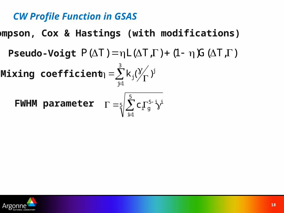
CW Profile Function in GSAS
Thompson, Cox & Hastings (with modifications)
Pseudo-Voigt ),T(G)1(),T(L)T(P
Mixing coefficient j3
1jj )(k
FWHM parameter 5
5
1i
ii5gic
19
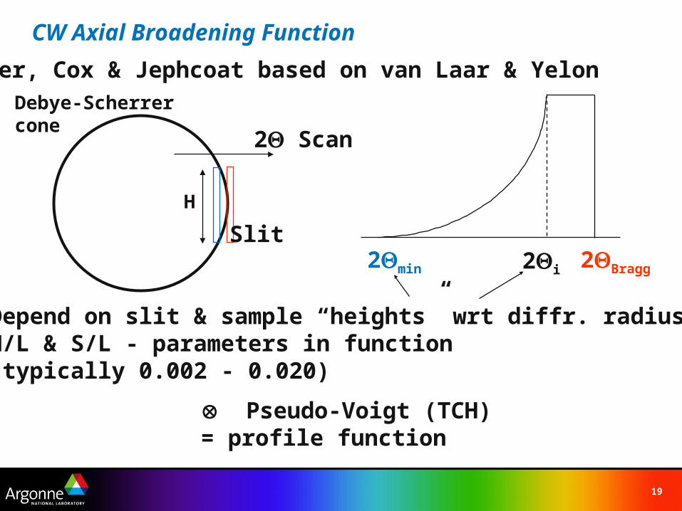
CW Axial Broadening Function
Finger, Cox & Jephcoat based on van Laar & Yelon
2Bragg2i2min
Pseudo-Voigt (TCH)= profile function
Depend on slit & sample “heights” wrt diffr. radiusH/L & S/L - parameters in function(typically 0.002 - 0.020)
Debye-Scherrer cone
2 Scan
Slit
H
20
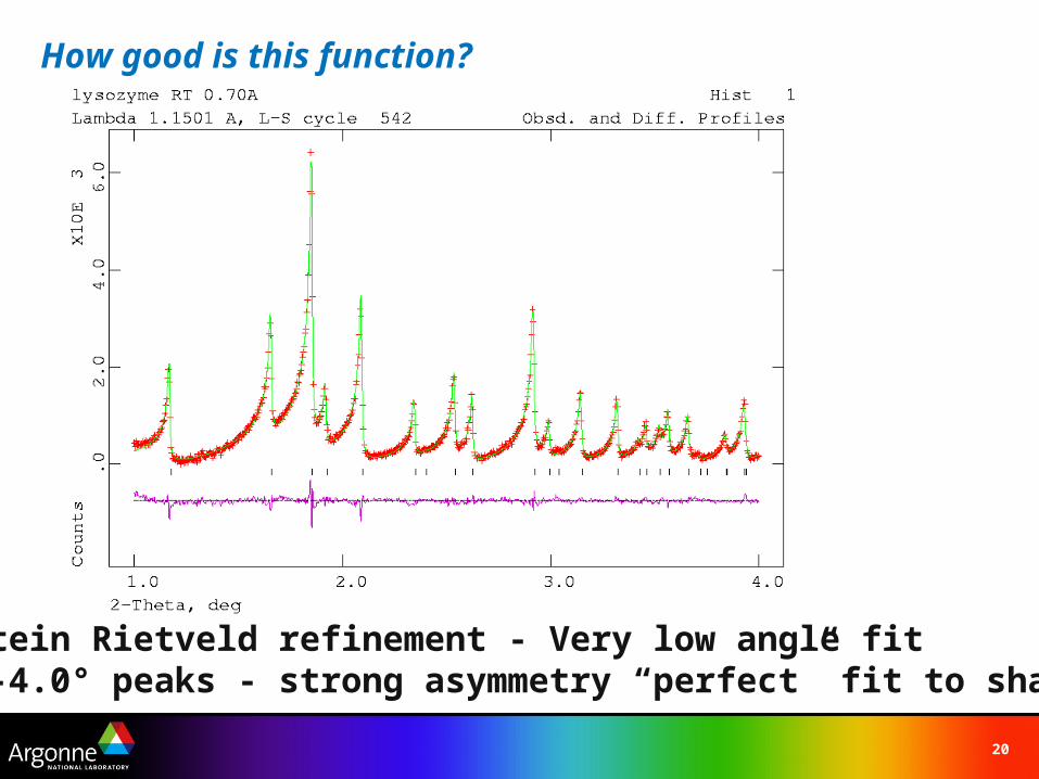
How good is this function?
Protein Rietveld refinement - Very low angle fit1.0-4.0° peaks - strong asymmetry “perfect” fit to shape
21
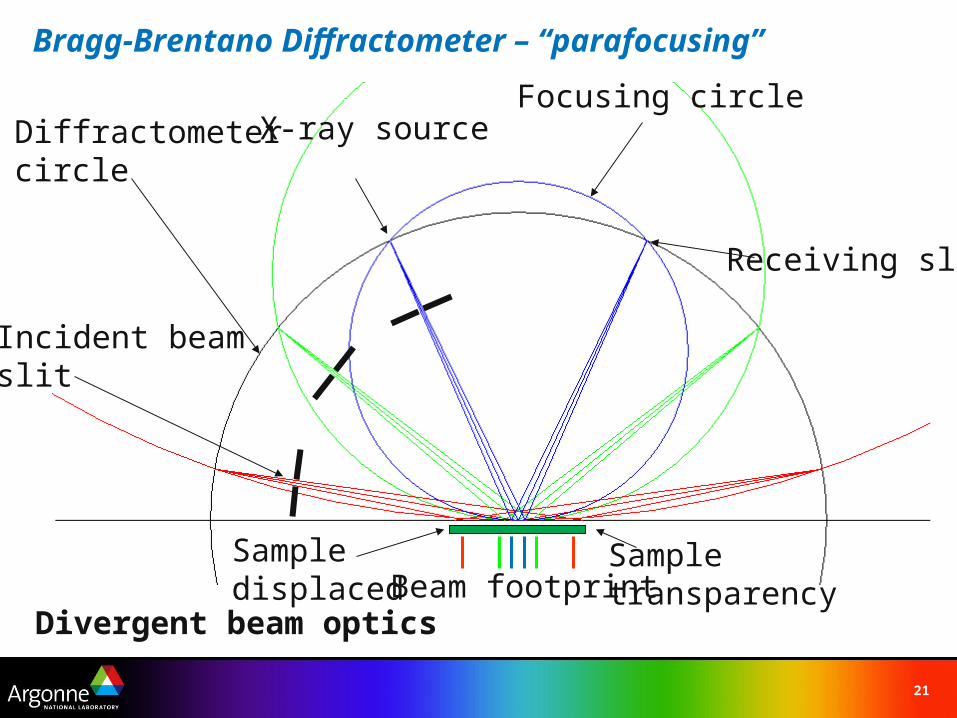
Bragg-Brentano Diffractometer – “parafocusing”
Diffractometercircle
Sampledisplaced
Receiving slit
X-ray sourceFocusing circle
Divergent beam optics
Incident beamslit
Beam footprintSample transparency
22
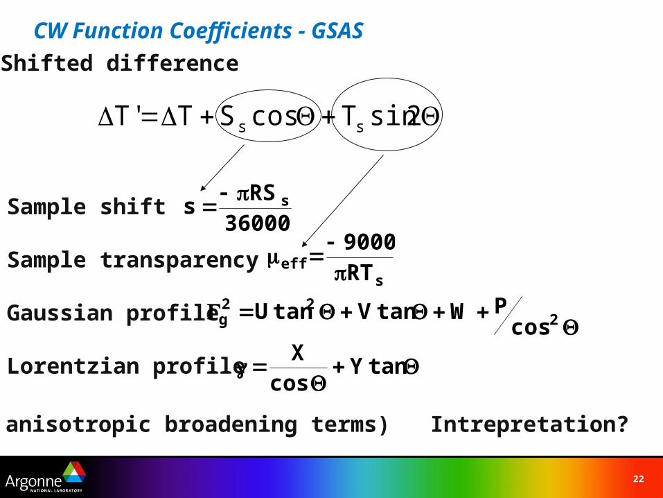
CW Function Coefficients - GSAS
Sample shift
Sample transparency
Gaussian profile
Lorentzian profile
36000RS
s s
seff RT
9000
2
22g cos
PWtanVtanU
tanYcos
X
(plus anisotropic broadening terms) Intrepretation?
Shifted difference
2sinTcosST'T ss
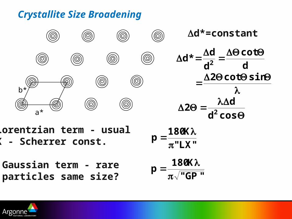
Crystallite Size Broadening
a*
b*
d*=constant
dcot
d
d*d 2
sincot2
cosd
d2 2
Lorentzian term - usualK - Scherrer const. "LX"
K180p
Gaussian term - rareparticles same size? "GP"
K180p
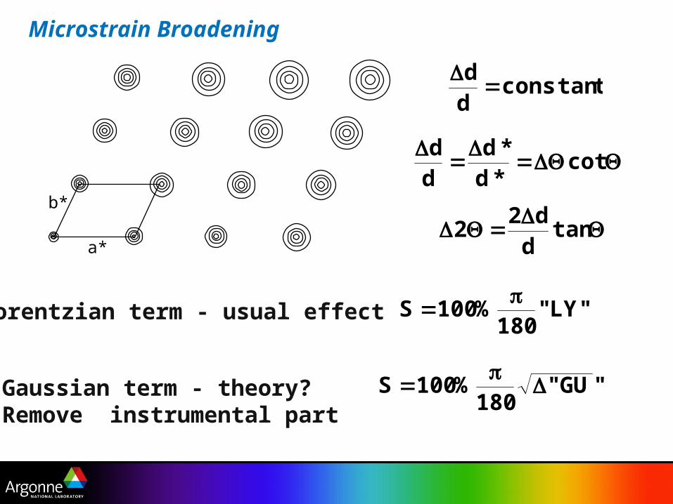
Microstrain Broadening
a*
b*
ttanconsdd
cot
*d*d
dd
tand
d22
Lorentzian term - usual effect "LY"180
%100S
Gaussian term - theory?Remove instrumental part
"GU"180
%100S
25
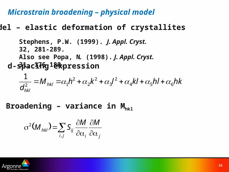
Microstrain broadening – physical model
Stephens, P.W. (1999). J. Appl. Cryst. 32, 281-289.Also see Popa, N. (1998). J. Appl. Cryst. 31, 176-180.
Model – elastic deformation of crystallites
hkhlkllkhMd hkl
hkl654
23
22
212
1
d-spacing expression
j,i ji
ijhkl
MMSM2
Broadening – variance in Mhkl
26
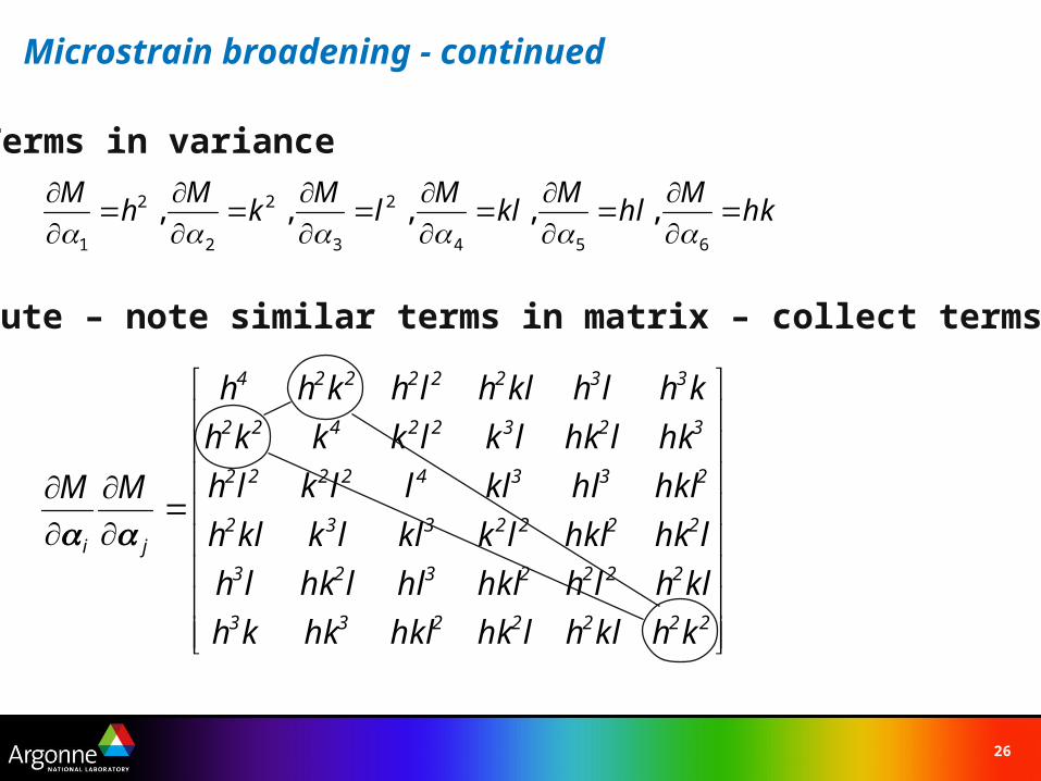
hkM
hlM
klM
lM
kM
hM
654
2
3
2
2
2
1
,,,,,
2222233
2222323
2222332
23342222
32322422
33222224
khklhlhkhklhkkh
klhlhhklhllhklh
lhkhkllkkllkklh
hklhlklllklh
hklhklklkkkh
khlhklhlhkhh
MM
ji
Microstrain broadening - continued
Terms in variance
Substitute – note similar terms in matrix – collect terms
27
42 LKH,lkhSMHKL
LKHHKLhkl
2
1122
1212
211
3013
3301
3130
3031
3103
3310
22022
22202
22220
4004
4040
4400
2
4
2
3
hklSlhkSklhS
klSlhShkSlkShlSkhS
lkSlhSkhSlSkShSM hkl
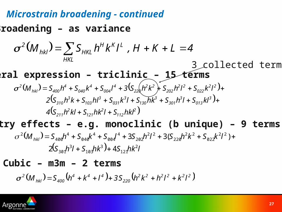
Microstrain broadening - continued
Broadening – as variance
General expression – triclinic – 15 terms
Symmetry effects – e.g. monoclinic (b unique) – 9 terms
lhkShkSlhS
lkSkhSlhSlSkShSM hkl
2121
3103
3301
22022
22220
22202
4004
4040
4400
2
42
)(33
3 collected terms
Cubic – m3m – 2 terms
222222220
444400
2 3 lklhkhSlkhSM hkl
28
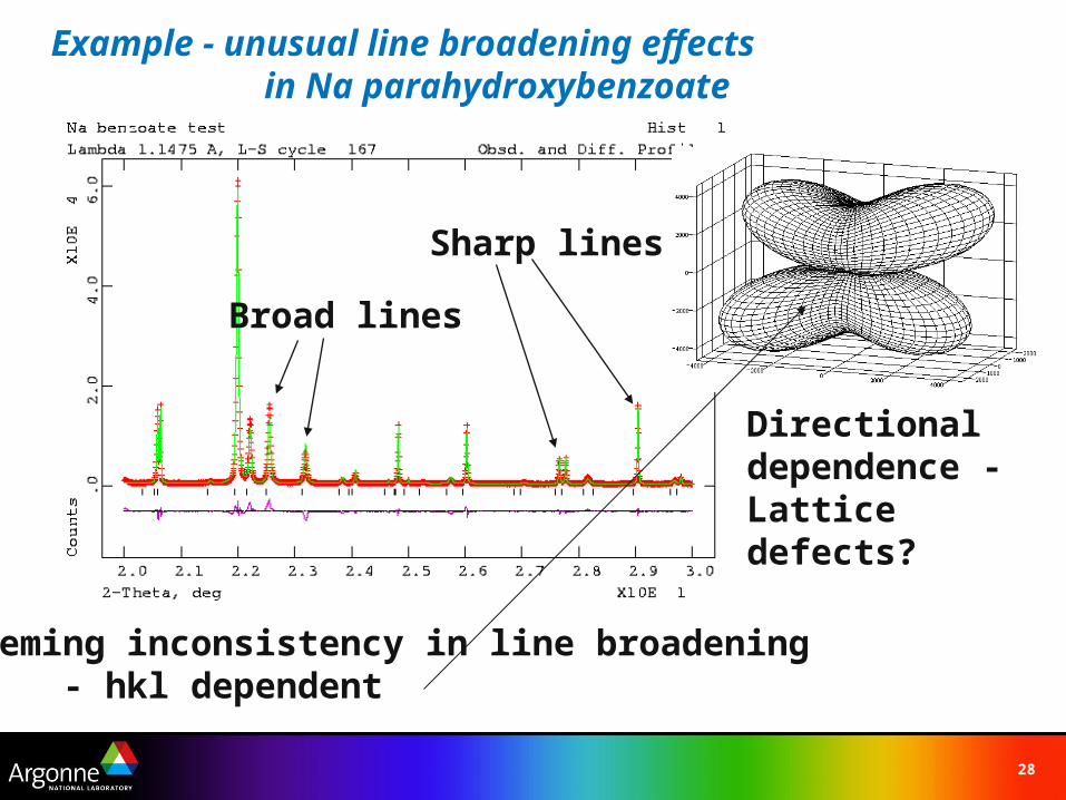
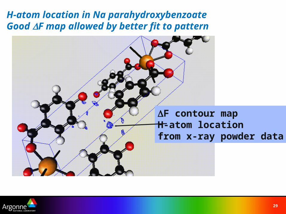
Example - unusual line broadening effects in Na parahydroxybenzoate
Sharp lines
Broad lines
Seeming inconsistency in line broadening- hkl dependent
Directional dependence - Lattice defects?
29
H-atom location in Na parahydroxybenzoateGood F map allowed by better fit to pattern
F contour mapH-atom locationfrom x-ray powder data
30
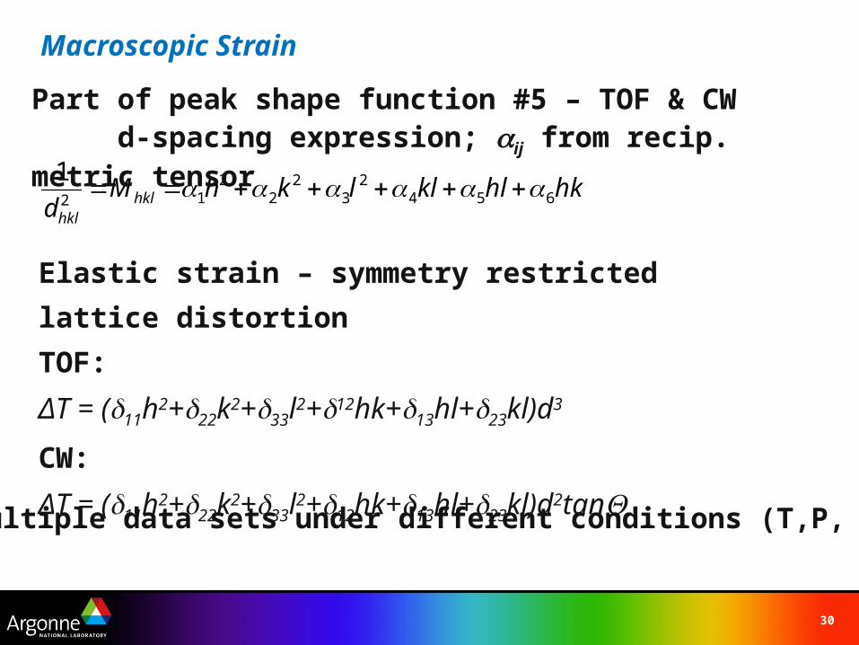
Macroscopic Strain
hkhlkllkhMd hkl
hkl654
23
22
212
1
Part of peak shape function #5 – TOF & CWd-spacing expression; ij from recip. metric tensor
Elastic strain – symmetry restricted lattice
distortion
TOF:
ΔT = (11h2+22k2+33l2+12hk+13hl+23kl)d3
CW:
ΔT = (11h2+22k2+33l2+12hk+13hl+23kl)d2tanWhy? Multiple data sets under different conditions (T,P, x, etc.)
31
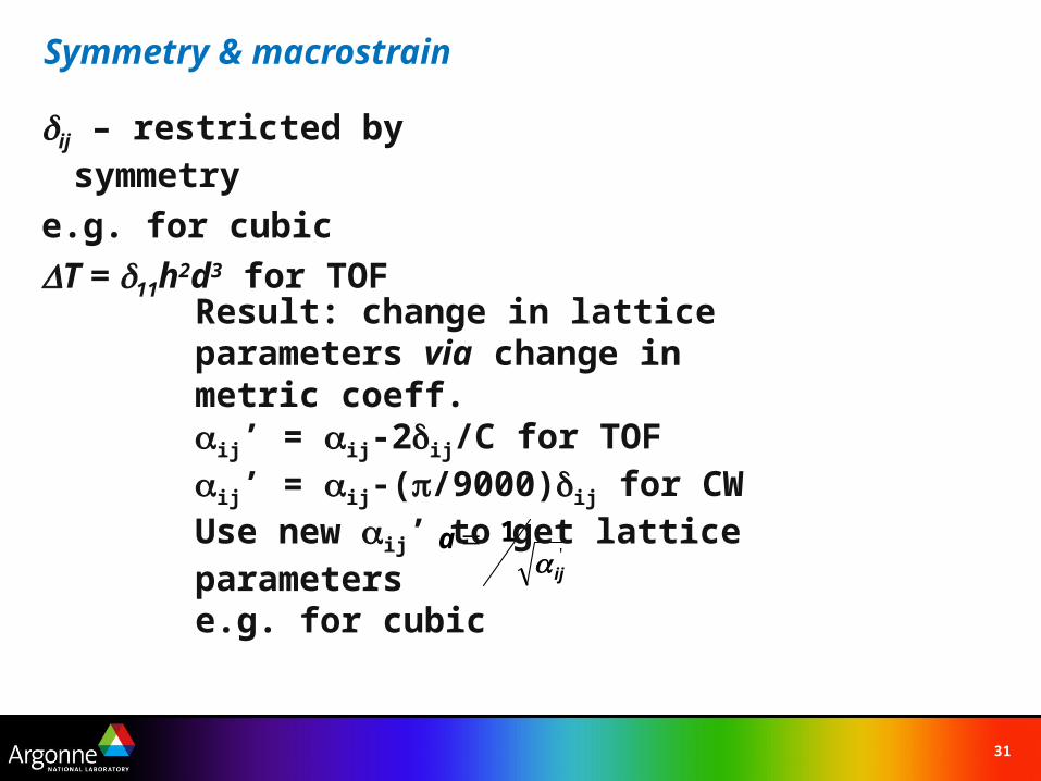
Symmetry & macrostrain
ij – restricted by symmetry
e.g. for cubic
T = 11h2d3 for TOF
'ij
a
1
Result: change in lattice parameters via change in metric coeff.ij’ = ij-2ij/C for TOFij’ = ij-(/9000)ij for CWUse new ij’ to get lattice parameterse.g. for cubic
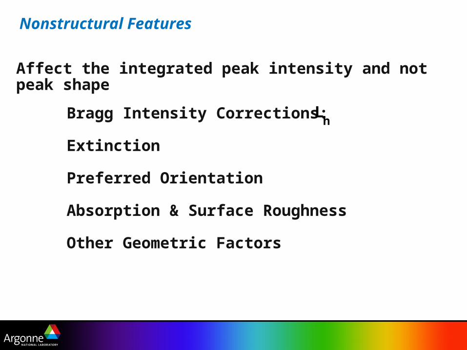
Bragg Intensity Corrections:
Extinction
Preferred Orientation
Absorption & Surface Roughness
Other Geometric Factors
Affect the integrated peak intensity and not peak shape
Lh
Nonstructural Features
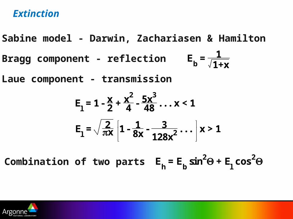
Sabine model - Darwin, Zachariasen & Hamilton
Bragg component - reflection
Laue component - transmission
Extinction
Eh = E
b sin2 + E
l cos2
Eb =
1+x1
Combination of two parts
El = 1 - 2
x + 4x2
- 485x3
. . . x < 1
El = x
2 1 - 8x
1 - 128x2
3 . . . x > 1
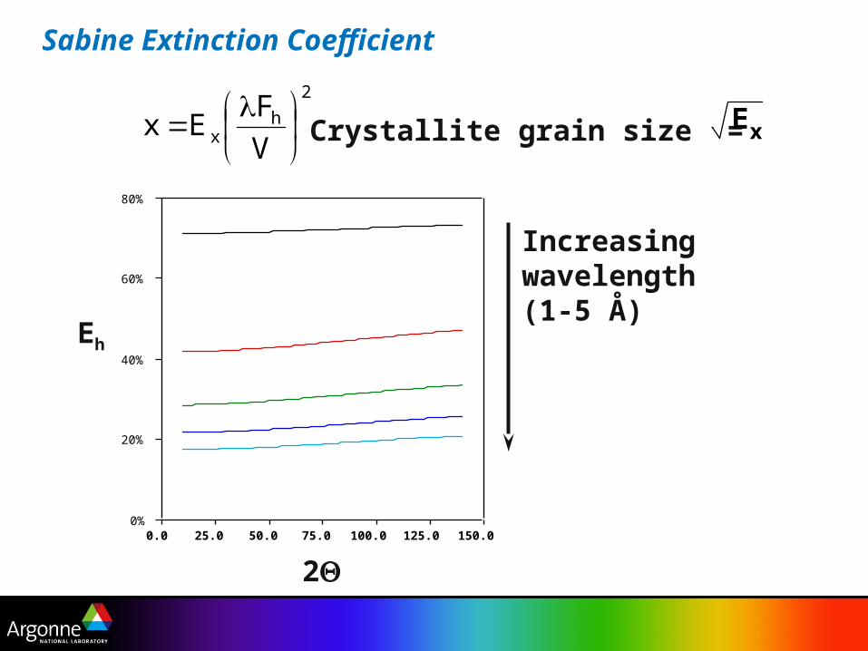
Sabine Extinction Coefficient
Crystallite grain size = Ex
2
0%
20%
40%
60%
80%
0.0 25.0 50.0 75.0 100.0 125.0 150.0
Eh
Increasingwavelength(1-5 Å)
2
hx V
FEx
35
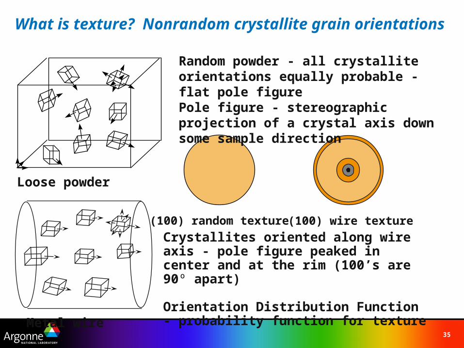
Random powder - all crystallite orientations equally probable - flat pole figure
Crystallites oriented along wire axis - pole figure peaked in center and at the rim (100’s are 90º apart)
Orientation Distribution Function - probability function for texture
(100) wire texture(100) random texture
What is texture? Nonrandom crystallite grain orientations
Pole figure - stereographic projection of a crystal axis down some sample direction
Loose powder
Metal wire
36
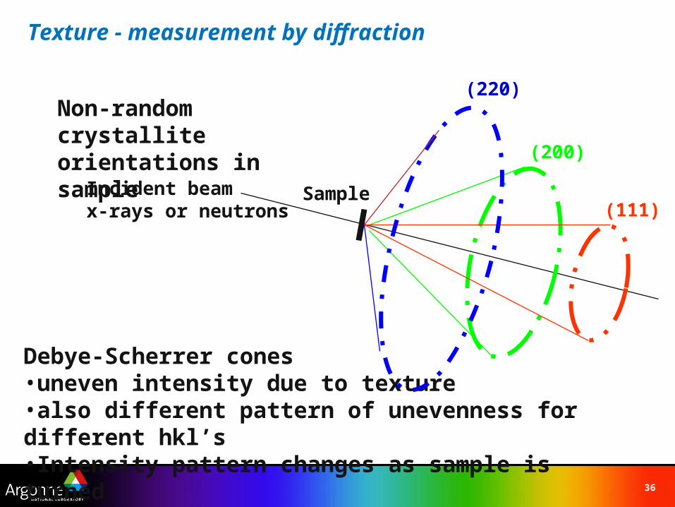
Texture - measurement by diffraction
Debye-Scherrer cones •uneven intensity due to texture •also different pattern of unevenness for different hkl’s•Intensity pattern changes as sample is turned
Non-random crystallite orientations in sample
Incident beamx-rays or neutrons
Sample(111)
(200)
(220)
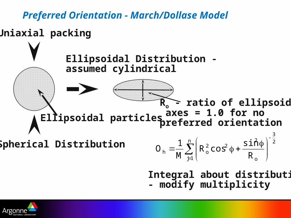
Spherical Distribution
Ellipsoidal Distribution -assumed cylindrical
Ellipsoidal particles
Uniaxial packing
Preferred Orientation - March/Dollase Model
Integral about distribution- modify multiplicity
Ro - ratio of ellipsoid axes = 1.0 for nopreferred orientation
2
3n
1j o
222
oh R
sincosR
M
1O
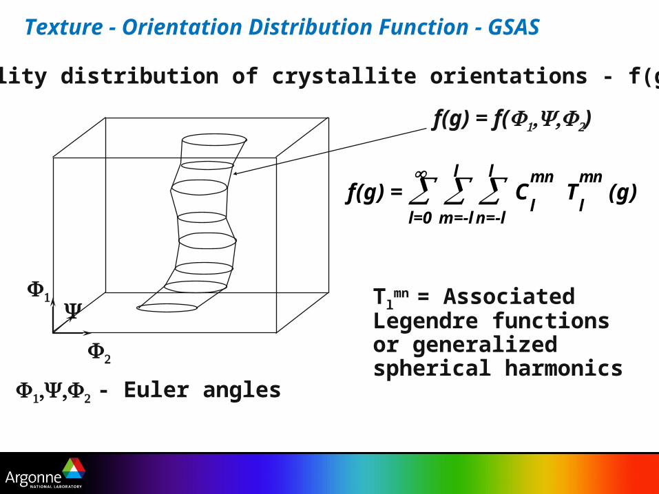
Texture - Orientation Distribution Function - GSAS
f(g) = l=0
m=-l
l n=-l
l C
l
mn T
l
mn (g)
Tlmn = Associated
Legendre functions or generalized spherical harmonics
- Euler angles
f(g) = f()
Probability distribution of crystallite orientations - f(g)
39
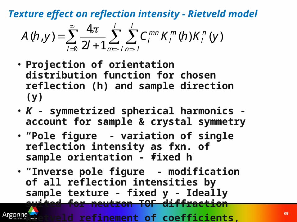
• Projection of orientation distribution function for chosen reflection (h) and sample direction (y)
• K - symmetrized spherical harmonics - account for sample & crystal symmetry
• “Pole figure” - variation of single reflection intensity as fxn. of sample orientation - fixed h
• “Inverse pole figure” - modification of all reflection intensities by sample texture - fixed y - Ideally suited for neutron TOF diffraction
• Rietveld refinement of coefficients, Clmn, and 3
orientation angles - sample alignment
Texture effect on reflection intensity - Rietveld model
)()(12
4),(
0
yKhKCl
yhA nl
ml
l
lm
l
ln
mnl
l
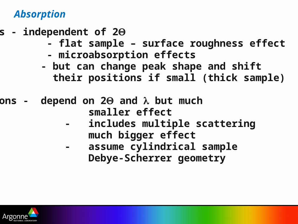
Absorption
X-rays - independent of 2 - flat sample – surface roughness effect - microabsorption effects - but can change peak shape and shift their positions if small (thick sample)
Neutrons - depend on 2 and but much smaller effect - includes multiple scattering much bigger effect - assume cylindrical sample Debye-Scherrer geometry
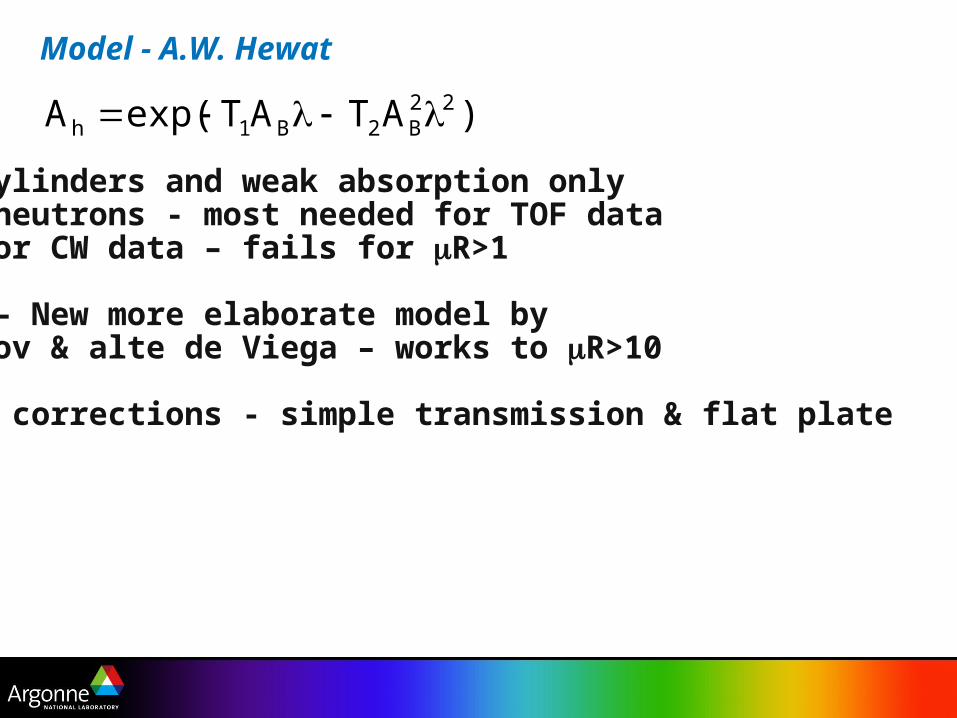
Model - A.W. Hewat
For cylinders and weak absorption onlyi.e. neutrons - most needed for TOF datanot for CW data – fails for R>1
GSAS – New more elaborate model by Lobanov & alte de Viega – works to R>10
Other corrections - simple transmission & flat plate
)ATATexp(A 22B2B1h
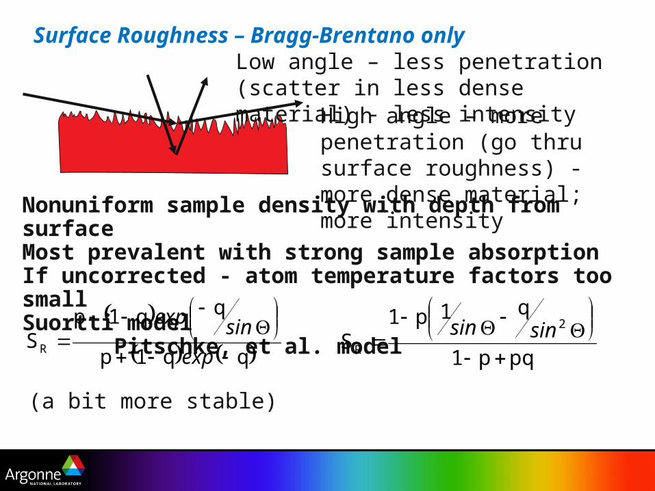
Nonuniform sample density with depth from surfaceMost prevalent with strong sample absorptionIf uncorrected - atom temperature factors too smallSuortti model Pitschke, et al. model
Surface Roughness – Bragg-Brentano only
High angle – more penetration (go thru surface roughness) - more dense material; more intensity
Low angle – less penetration (scatter in less dense material) - less intensity
pqp1
q1p1S
2
R
sinsin qq1p
qq1pSR
exp
sinexp
(a bit more stable)
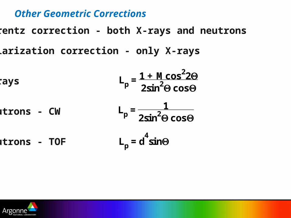
Other Geometric Corrections
Lorentz correction - both X-rays and neutrons
Polarization correction - only X-rays
X-rays
Neutrons - CW
Neutrons - TOF
Lp = 2sin2 cos1 + M cos22
Lp = 2sin2 cos
1
Lp = d4sin
44
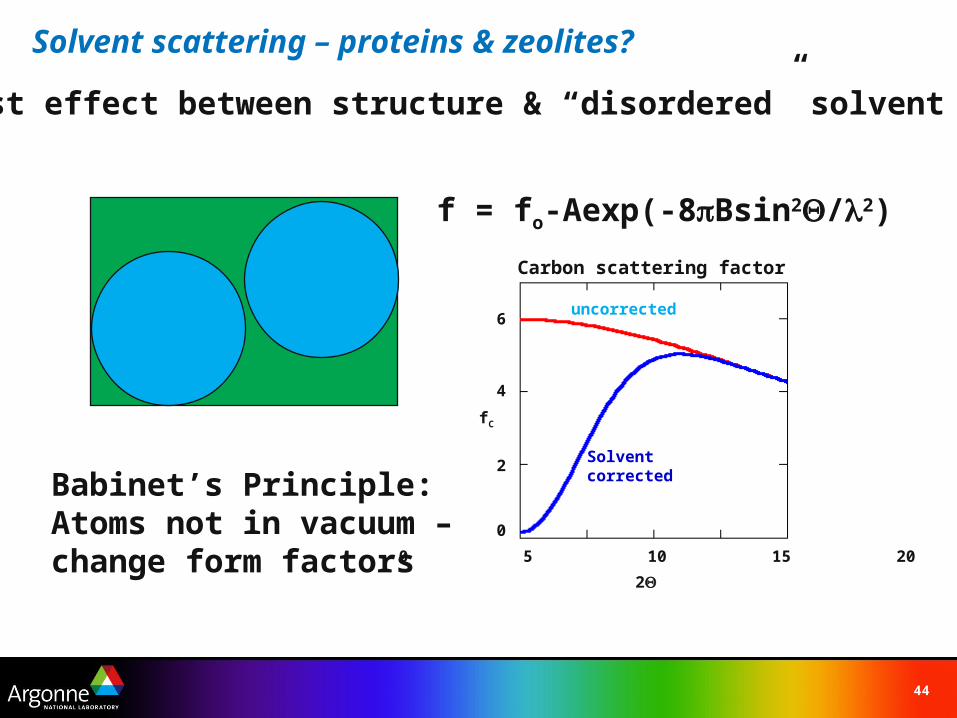
Solvent scattering – proteins & zeolites?
Contrast effect between structure & “disordered” solvent region
Babinet’s Principle:Atoms not in vacuum – change form factors
f = fo-Aexp(-8Bsin2/2)
0
2
4
6
0 5 10 15 20
2
fC
uncorrected
Solvent corrected
Carbon scattering factor
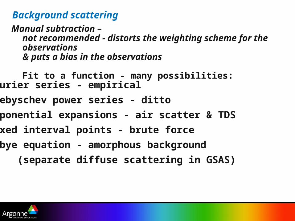
Manual subtraction – not recommended - distorts the weighting scheme for the observations& puts a bias in the observations
Fit to a function - many possibilities:
Fourier series - empirical
Chebyschev power series - ditto
Exponential expansions - air scatter & TDS
Fixed interval points - brute force
Debye equation - amorphous background
(separate diffuse scattering in GSAS)
Background scattering
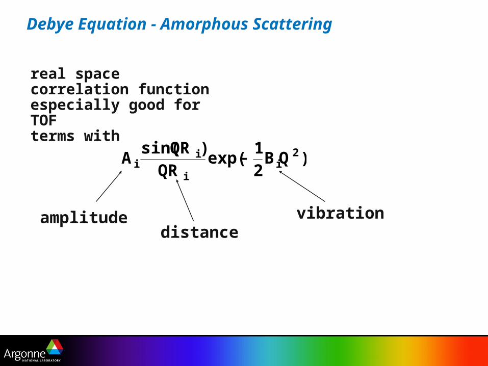
real space correlation functionespecially good for TOFterms with
Debye Equation - Amorphous Scattering
)QB21
exp(QR
)QRsin(A 2
ii
ii
amplitudedistance
vibration
47
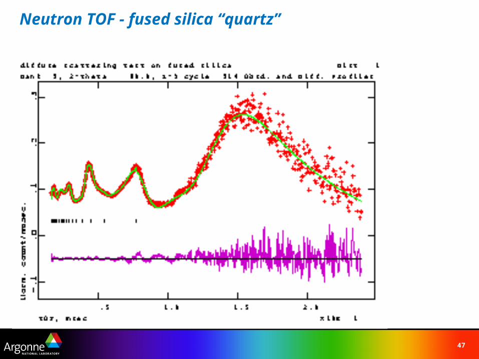
Neutron TOF - fused silica “quartz”
48
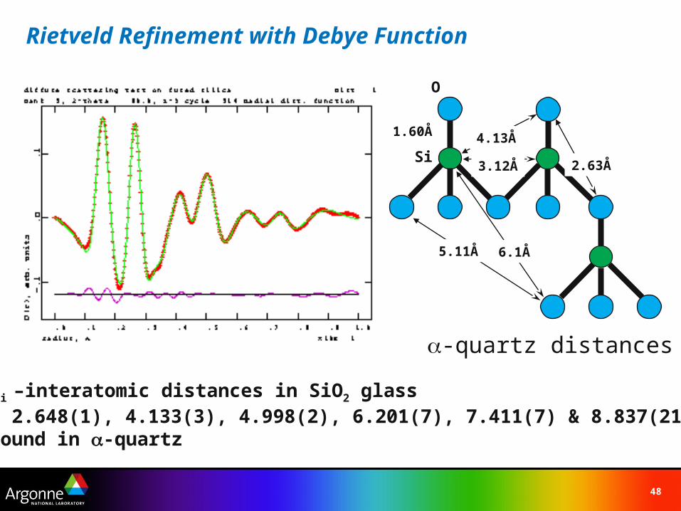
Rietveld Refinement with Debye Function
7 terms Ri –interatomic distances in SiO2 glass 1.587(1), 2.648(1), 4.133(3), 4.998(2), 6.201(7), 7.411(7) & 8.837(21)Same as found in -quartz
1.60Å
Si
O
4.13Å
2.63Å3.12Å
5.11Å 6.1Å
-quartz distances
Summary
Non-Structural Features in Powder Patterns
1. Large crystallite size - extinction
2. Preferred orientation
3. Small crystallite size - peak shape
4. Microstrain (defect concentration)
5. Amorphous scattering - background
50
Time to quit?
Stephens’ Law –
“A Rietveld refinement is never perfected,
merely abandoned”
Also – “stop when you’ve run out of things to vary”
What if problem is more complex?
Apply constraints & restraints
“What to do when you have
too many parameters
& not enough data”
51
Complex structures (even proteins)
Too many parameters – “free” refinement failsKnown stereochemistry:Bond distancesBond anglesTorsion angles (less definite)Group planarity (e.g. phenyl groups)Chiral centers – handednessEtc.
Choice: rigid body description – fixed geometry/fewer parametersstereochemical restraints – more data
52
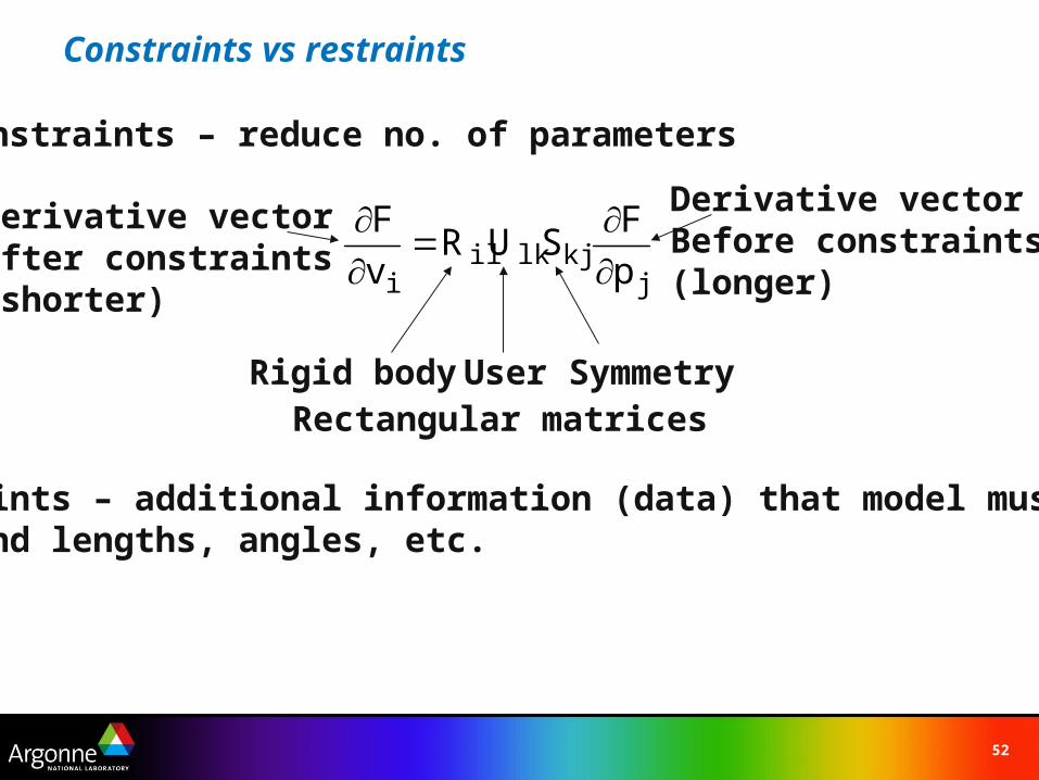
Constraints vs restraints
Constraints – reduce no. of parameters
jkjlkil
i p
FSUR
v
F
Rigid body User Symmetry
Derivative vectorBefore constraints(longer)
Derivative vectorAfter constraints(shorter)
Rectangular matrices
Restraints – additional information (data) that model must fitEx. Bond lengths, angles, etc.

53
Space group symmetry constraints
Special positions – on symmetry elementsAxes, mirrors & inversion centers (not glides & screws)Restrictions on refineable parametersSimple example: atom on inversion center – fixed x,y,zWhat about Uij’s?
– no restriction – ellipsoid has inversion center
Mirrors & axes ? – depends on orientation
Example: P 2/m – 2 || b-axis, m 2-fold
on 2-fold: x,z – fixed & U11,U22,U33, & U13 variableon m: y fixed & U11,U22, U33, & U13 variableRietveld programs – GSAS automatic, others not
54
Multi-atom site fractions
“site fraction” – fraction of site occupied by atom“site multiplicity”- no. times site occurs in cell“occupancy” – site fraction * site multiplicity
may be normalized by max multiplicity
GSAS uses fraction & multiplicity derived from sp. gp.Others use occupancy
If two atoms in site – Ex. Fe/Mg in olivineThen (if site full) FMg = 1-FFe
55
If 3 atoms A,B,C on site – problem
Diffraction experiment – relative scattering power of site
“1-equation & 2-unknowns” unsolvable problem
Need extra information to solve problem –
2nd diffraction experiment – different scattering power
“2-equations & 2-unknowns” problem
Constraint: solution of J.-M. Joubert
Add an atom – site has 4 atoms A, B, C, C’
so that FA+FB+FC+FC’=1
Then constrain so FA = -FC and FB = -FC’
Multi-atom site fractions - continued
56
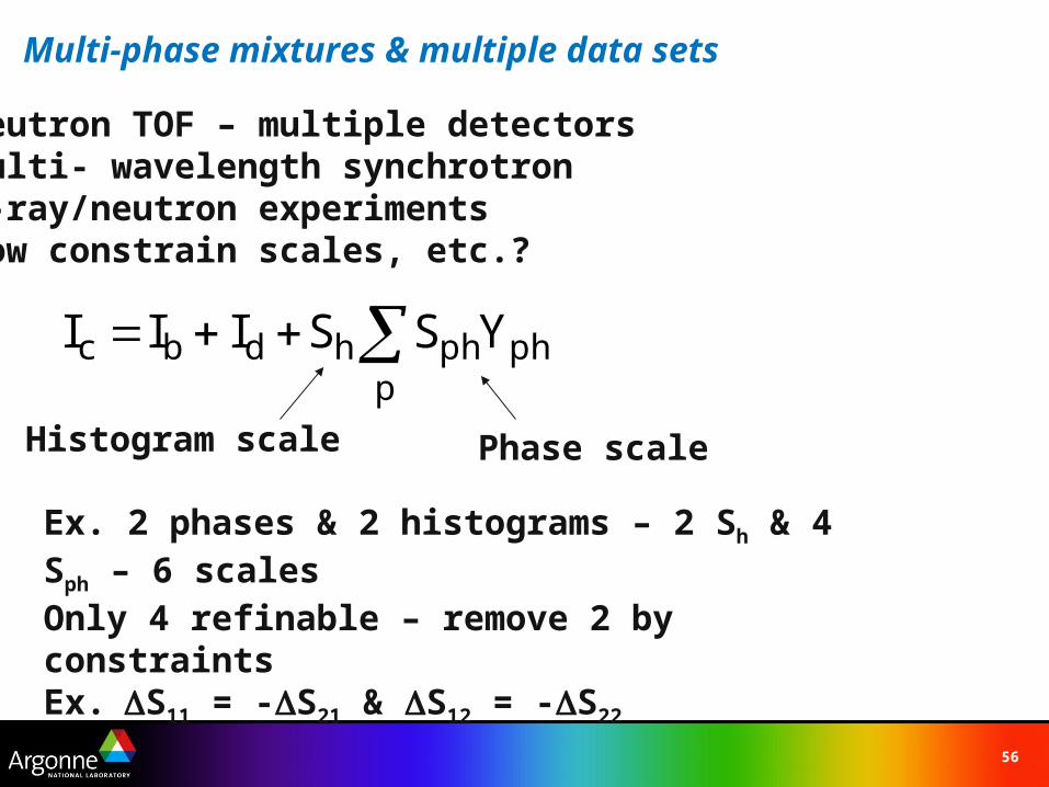
Multi-phase mixtures & multiple data sets
Neutron TOF – multiple detectorsMulti- wavelength synchrotronX-ray/neutron experimentsHow constrain scales, etc.?
p
phphhdbc YSSIII
Histogram scale Phase scale
Ex. 2 phases & 2 histograms – 2 Sh & 4 Sph – 6 scalesOnly 4 refinable – remove 2 by constraintsEx.S11 = -S21 & S12 = -S22
57
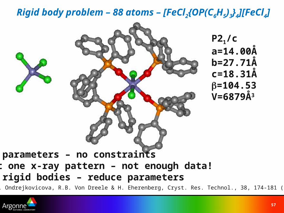
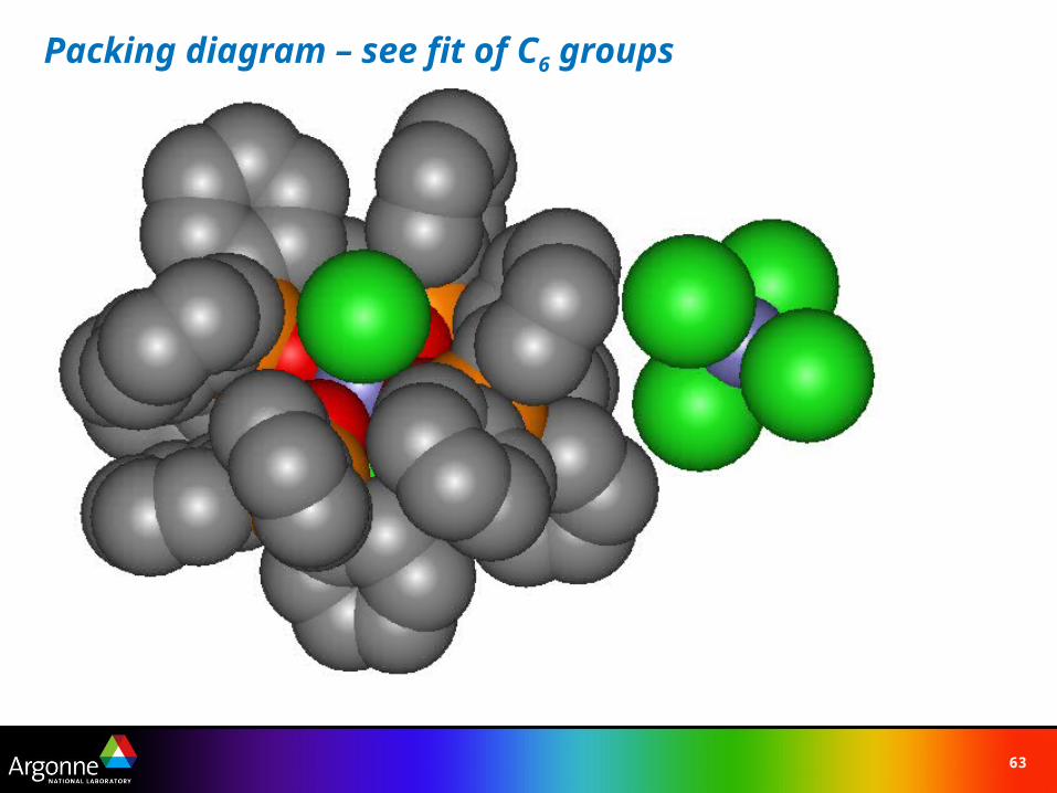
Rigid body problem – 88 atoms – [FeCl2{OP(C6H5)3}4][FeCl4]
264 parameters – no constraintsJust one x-ray pattern – not enough data!Use rigid bodies – reduce parameters
P21/ca=14.00Åb=27.71Åc=18.31Å=104.53V=6879Å3
V. Jorik, I. Ondrejkovicova, R.B. Von Dreele & H. Eherenberg, Cryst. Res. Technol., 38, 174-181 (2003)
58
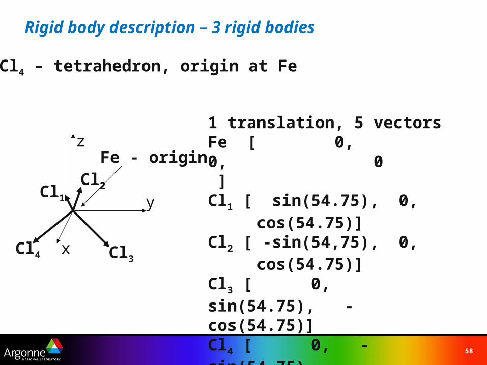
Rigid body description – 3 rigid bodies
FeCl4 – tetrahedron, origin at Fe
z
x
y
Fe - origin
Cl1
Cl2
Cl3Cl4
1 translation, 5 vectorsFe [ 0, 0, 0 ]Cl1 [ sin(54.75), 0, cos(54.75)]Cl2 [ -sin(54,75), 0, cos(54.75)]Cl3 [ 0, sin(54.75), -cos(54.75)]Cl4 [ 0, -sin(54.75), -cos(54.75)]D=2.1Å; Fe-Cl bond
59
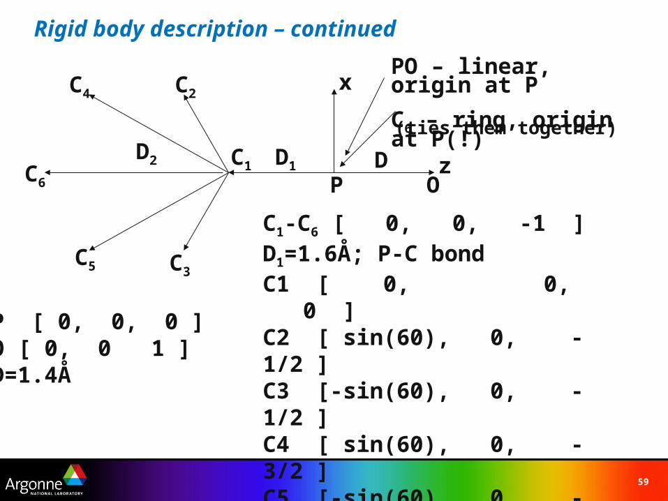
PO – linear, origin at P
C6 – ring, origin at P(!)
Rigid body description – continued
P OC1
C5 C3
C4 C2
C6z
x
P [ 0, 0, 0 ]O [ 0, 0 1 ]D=1.4Å
C1-C6 [ 0, 0, -1 ]D1=1.6Å; P-C bondC1 [ 0, 0, 0 ]C2 [ sin(60), 0, -1/2 ]C3 [-sin(60), 0, -1/2 ]C4 [ sin(60), 0, -3/2 ]C5 [-sin(60), 0, -3/2 ]C6 [ 0, 0, -2 ]D2=1.38Å; C-C aromatic bond
DD1D2
(ties them together)
60
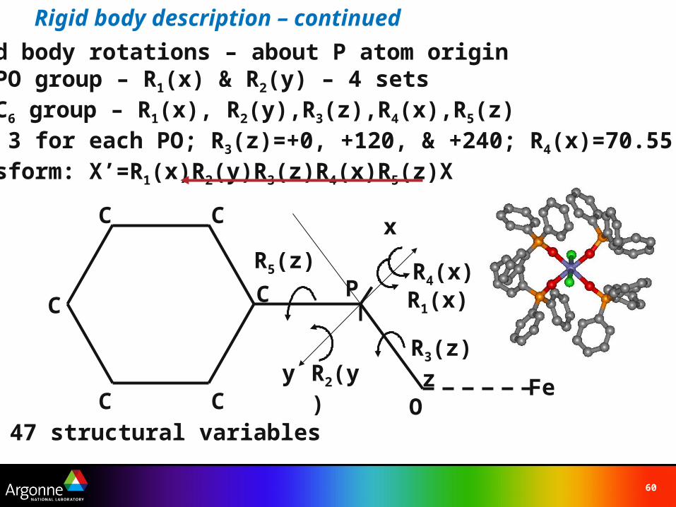
Rigid body description – continued
Rigid body rotations – about P atom originFor PO group – R1(x) & R2(y) – 4 setsFor C6 group – R1(x), R2(y),R3(z),R4(x),R5(z)
3 for each PO; R3(z)=+0, +120, & +240; R4(x)=70.55Transform: X’=R1(x)R2(y)R3(z)R4(x)R5(z)X
47 structural variables
P
O
C
C C
C C
C
z
x
y
R1(x)
R2(y)R3(z)
R5(z) R4(x)
Fe

61
Refinement - results
Rwp=4.49%Rp =3.29%RF
2 =9.98%Nrb =47Ntot =69
62
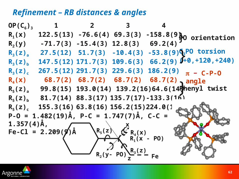
Refinement – RB distances & angles
OP(C6)3 1 2 3 4R1(x) 122.5(13) -76.6(4) 69.3(3) -158.8(9) R2(y) -71.7(3) -15.4(3) 12.8(3) 69.2(4)R3(z)a 27.5(12) 51.7(3) -10.4(3) -53.8(9)R3(z)b 147.5(12) 171.7(3) 109.6(3) 66.2(9)R3(z)c 267.5(12) 291.7(3) 229.6(3) 186.2(9)R4(x) 68.7(2) 68.7(2) 68.7(2) 68.7(2)R5(z)a 99.8(15) 193.0(14) 139.2(16) 64.6(14)R5(z)b 81.7(14) 88.3(17) 135.7(17) -133.3(16)R5(z)c 155.3(16) 63.8(16) 156.2(15) 224.0(16)P-O = 1.482(19)Å, P-C = 1.747(7)Å, C-C = 1.357(4)Å, Fe-Cl = 2.209(9)Å
z
x
R1(x - PO)
R2(y- PO)R3(z)
R5(z) R4(x)
Fe
}Phenyl twist
− C-P-O angle
C3PO torsion(+0,+120,+240)
} PO orientation
}
63
Packing diagram – see fit of C6 groups
64
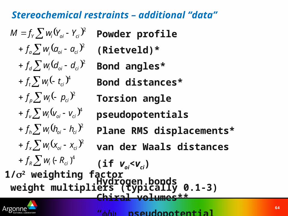
Stereochemical restraints – additional “data”
4
2
2
4
2
4
2
2
2
)( ciiR
cioiix
cioiih
cioiiv
ciip
ciit
cioiid
cioiia
cioiiY
Rwf
xxwf
hhwf
vvwf
pwf
twf
ddwf
aawf
YYwfM
Powder profile (Rietveld)*
Bond angles*
Bond distances*
Torsion angle pseudopotentials
Plane RMS displacements*
van der Waals distances (if voi<vci)
Hydrogen bonds
Chiral volumes**
“” pseudopotentialwi = 1/2 weighting factorfx - weight multipliers (typically 0.1-3)
65
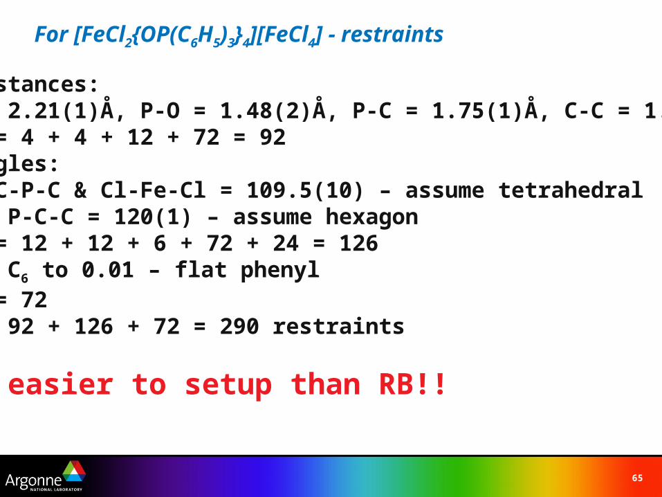
For [FeCl2{OP(C6H5)3}4][FeCl4] - restraints
Bond distances: Fe-Cl = 2.21(1)Å, P-O = 1.48(2)Å, P-C = 1.75(1)Å, C-C = 1.36(1)ÅNumber = 4 + 4 + 12 + 72 = 92Bond angles:O-P-C, C-P-C & Cl-Fe-Cl = 109.5(10) – assume tetrahedralC-C-C & P-C-C = 120(1) – assume hexagonNumber = 12 + 12 + 6 + 72 + 24 = 126Planes: C6 to 0.01 – flat phenylNumber = 72Total = 92 + 126 + 72 = 290 restraints
A lot easier to setup than RB!!
66
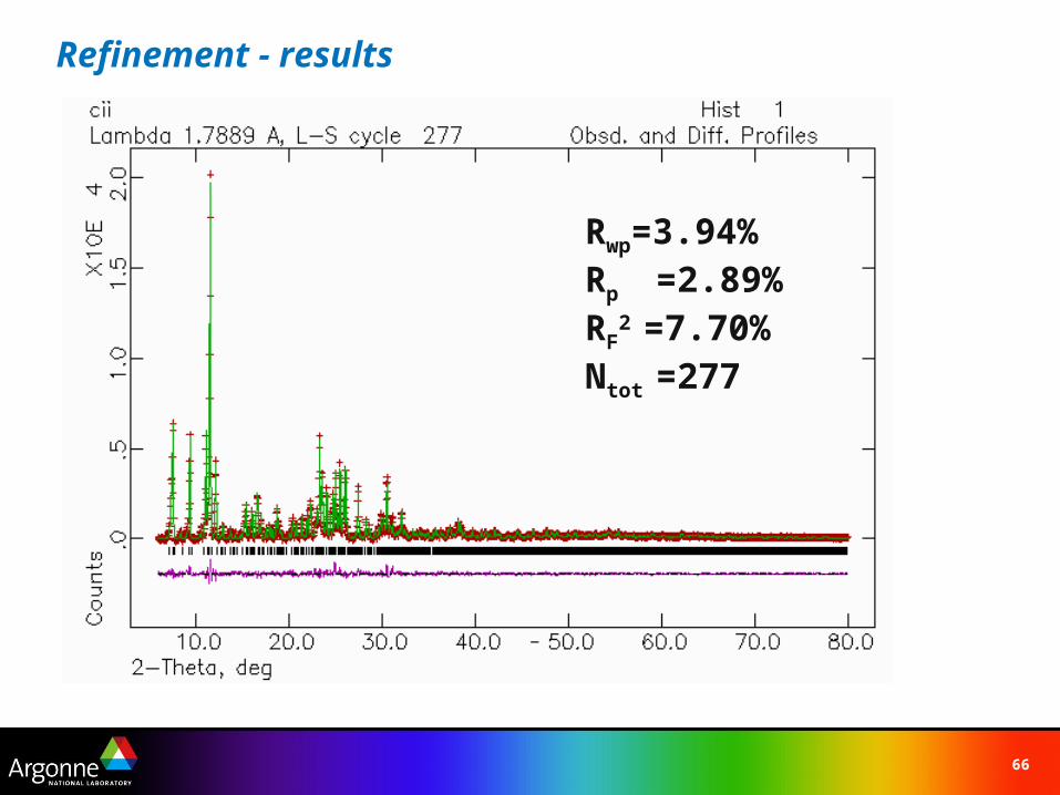
Refinement - results
Rwp=3.94%Rp =2.89%RF
2 =7.70%Ntot =277
67
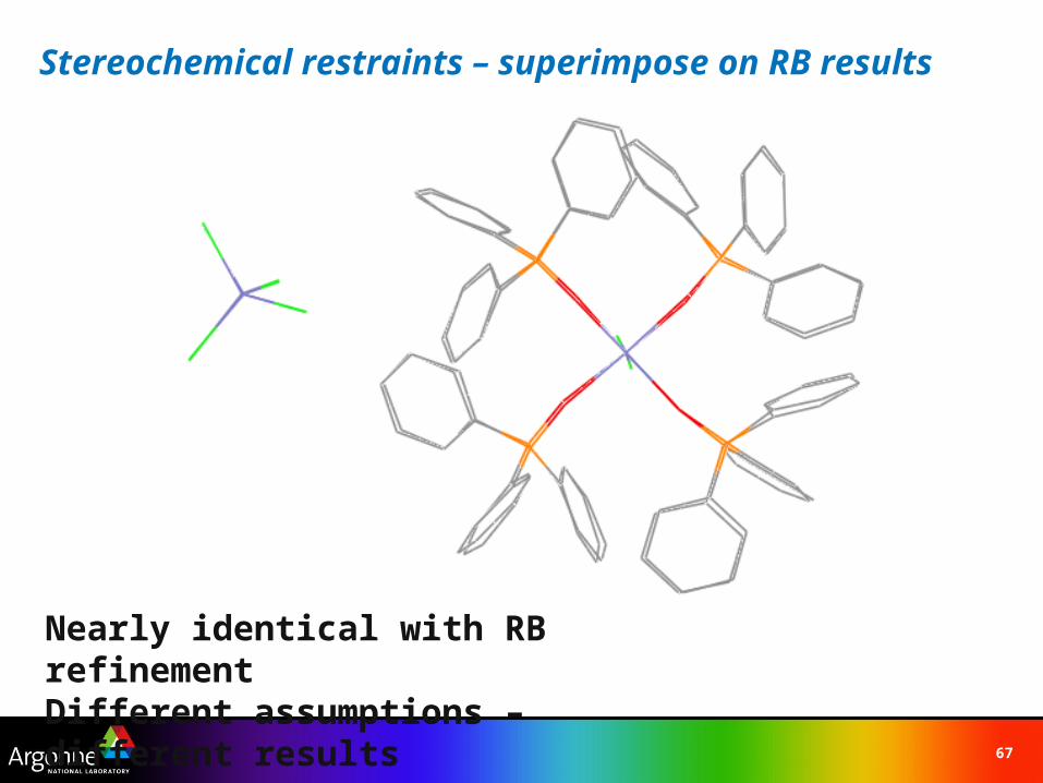
Stereochemical restraints – superimpose on RB results
Nearly identical with RB refinementDifferent assumptions – different results
68
New rigid bodies for proteins (actually more general)
Proteins have too many parameters
Poor data/parameter ratio - especially for powder data
Very well known amino acid bonding –
e.g. Engh & Huber
Reduce “free” variables – fixed bond lengths & angles
Define new objects for protein structure –
flexible rigid bodies for amino acid residues
Focus on the “real” variables –
location/orientation & torsion angles of each residue
Parameter reduction ~1/3 of original protein xyz set
69
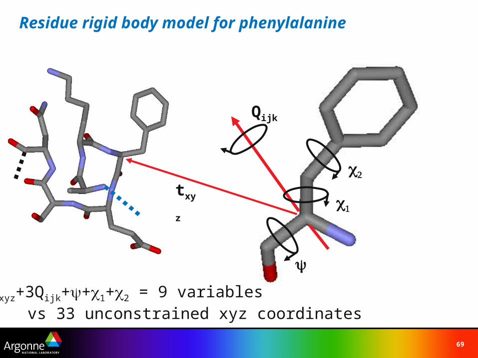
txyz
Qijk
Residue rigid body model for phenylalanine
3txyz+3Qijk++1+2 = 9 variables vs 33 unconstrained xyz coordinates
70
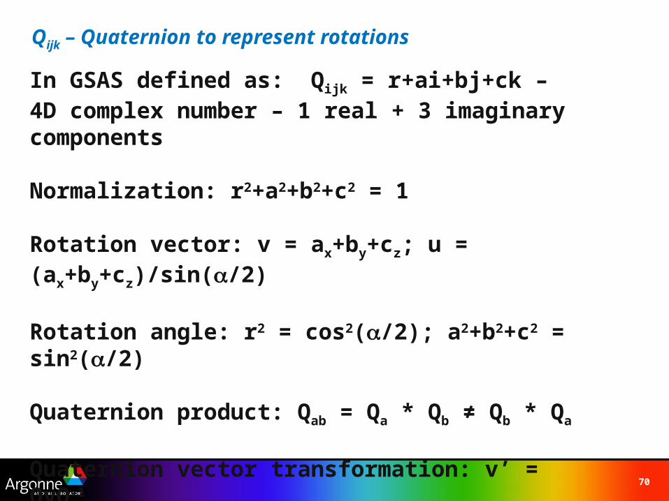
Qijk – Quaternion to represent rotations
In GSAS defined as: Qijk = r+ai+bj+ck – 4D complex number – 1 real + 3 imaginary components
Normalization: r2+a2+b2+c2 = 1
Rotation vector: v = ax+by+cz; u = (ax+by+cz)/sin(/2)
Rotation angle: r2 = cos2(/2); a2+b2+c2 = sin2(/2)
Quaternion product: Qab = Qa * Qb ≠ Qb * Qa
Quaternion vector transformation: v’ = QvQ-1
71
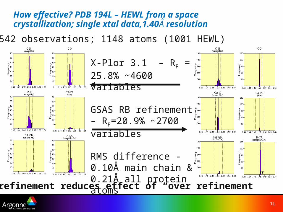
How effective? PDB 194L – HEWL from a space crystallization; single xtal data,1.40Å resolution
X-Plor 3.1 – RF = 25.8% ~4600 variables
GSAS RB refinement – RF=20.9% ~2700 variables
RMS difference - 0.10Å main chain & 0.21Å all protein atoms
21542 observations; 1148 atoms (1001 HEWL)
RB refinement reduces effect of “over refinement”
72
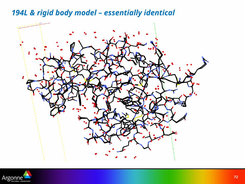
194L & rigid body model – essentially identical
73
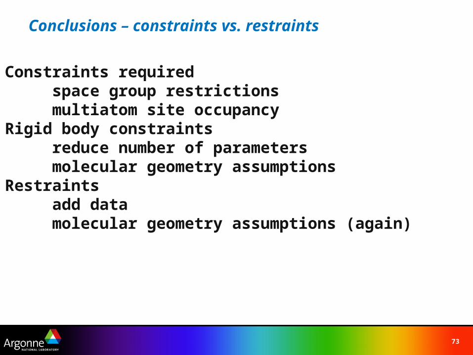
Conclusions – constraints vs. restraints
Constraints required space group restrictionsmultiatom site occupancy
Rigid body constraintsreduce number of parametersmolecular geometry assumptions
Restraintsadd datamolecular geometry assumptions (again)
74
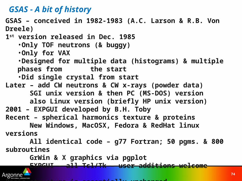
GSAS - A bit of historyGSAS – conceived in 1982-1983 (A.C. Larson & R.B. Von Dreele)1st version released in Dec. 1985
•Only TOF neutrons (& buggy) •Only for VAX•Designed for multiple data (histograms) & multiple phases from
the start•Did single crystal from start
Later – add CW neutrons & CW x-rays (powder data)SGI unix version & then PC (MS-DOS) versionalso Linux version (briefly HP unix version)
2001 – EXPGUI developed by B.H. TobyRecent – spherical harmonics texture & proteins
New Windows, MacOSX, Fedora & RedHat linux versionsAll identical code – g77 Fortran; 50 pgms. & 800 subroutinesGrWin & X graphics via pgplotEXPGUI – all Tcl/Tk – user additions welcome
Basic structure is essentially unchanged
75
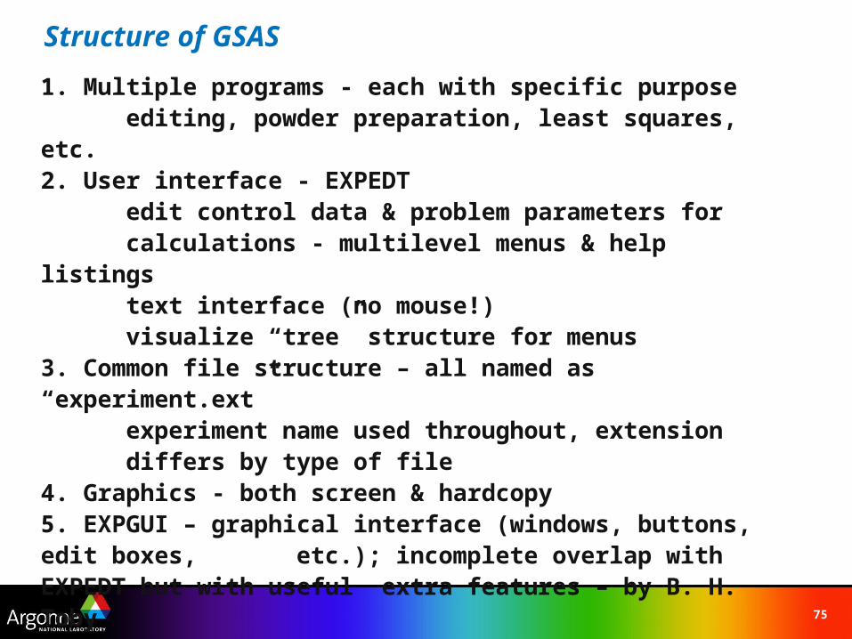
Structure of GSAS
1. Multiple programs - each with specific purposeediting, powder preparation, least squares, etc.
2. User interface - EXPEDTedit control data & problem parameters forcalculations - multilevel menus & help listingstext interface (no mouse!)visualize “tree” structure for menus
3. Common file structure – all named as “experiment.ext”experiment name used throughout, extensiondiffers by type of file
4. Graphics - both screen & hardcopy5. EXPGUI – graphical interface (windows, buttons, edit boxes,
etc.); incomplete overlap with EXPEDT but with useful extra features – by B. H. Toby
76
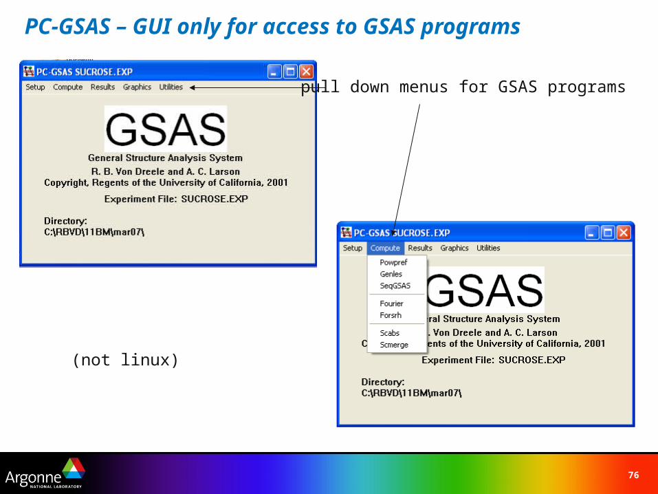
PC-GSAS – GUI only for access to GSAS programs
pull down menus for GSAS programs
(not linux)
77
GSAS & EXPGUI interfaces
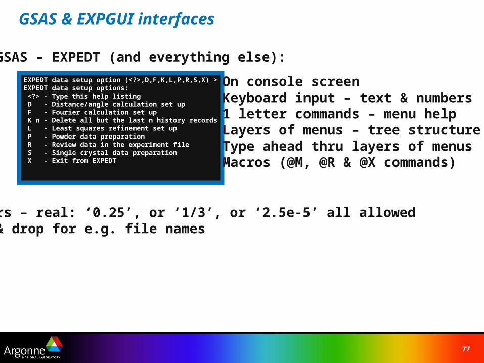
EXPEDT data setup option (<?>,D,F,K,L,P,R,S,X) >EXPEDT data setup options: <?> - Type this help listing D - Distance/angle calculation set up F - Fourier calculation set up K n - Delete all but the last n history records L - Least squares refinement set up P - Powder data preparation R - Review data in the experiment file S - Single crystal data preparation X - Exit from EXPEDT
On console screenKeyboard input – text & numbers1 letter commands – menu helpLayers of menus – tree structureType ahead thru layers of menusMacros (@M, @R & @X commands)
GSAS – EXPEDT (and everything else):
Numbers – real: ‘0.25’, or ‘1/3’, or ‘2.5e-5’ all allowedDrag & drop for e.g. file names
78
GSAS & EXPGUI interfaces
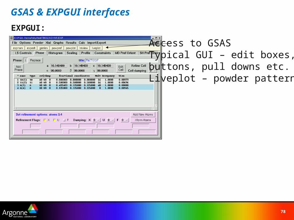
EXPGUI:
Access to GSASTypical GUI – edit boxes,buttons, pull downs etc.Liveplot – powder pattern
79
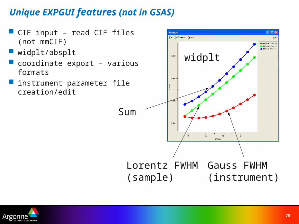
Unique EXPGUI features (not in GSAS)
CIF input – read CIF files (not mmCIF) widplt/absplt coordinate export – various formats instrument parameter file creation/edit
Gauss FWHM(instrument)
Lorentz FWHM(sample)
Sum
widplt
80
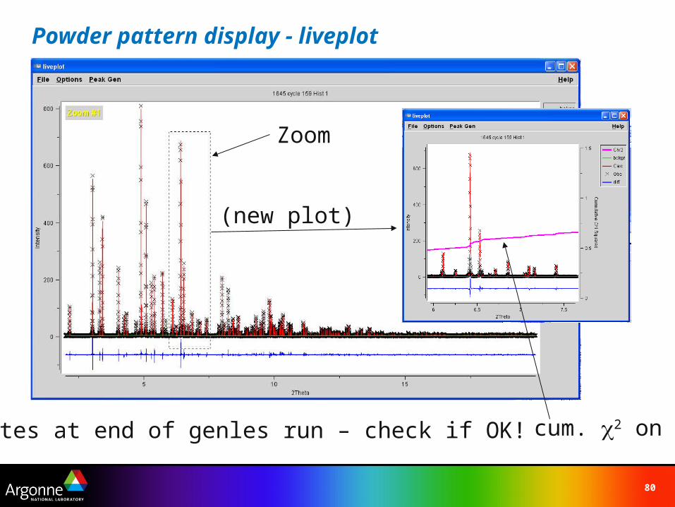
Powder pattern display - liveplot
Zoom
(new plot)
cum. 2 onupdates at end of genles run – check if OK!
81
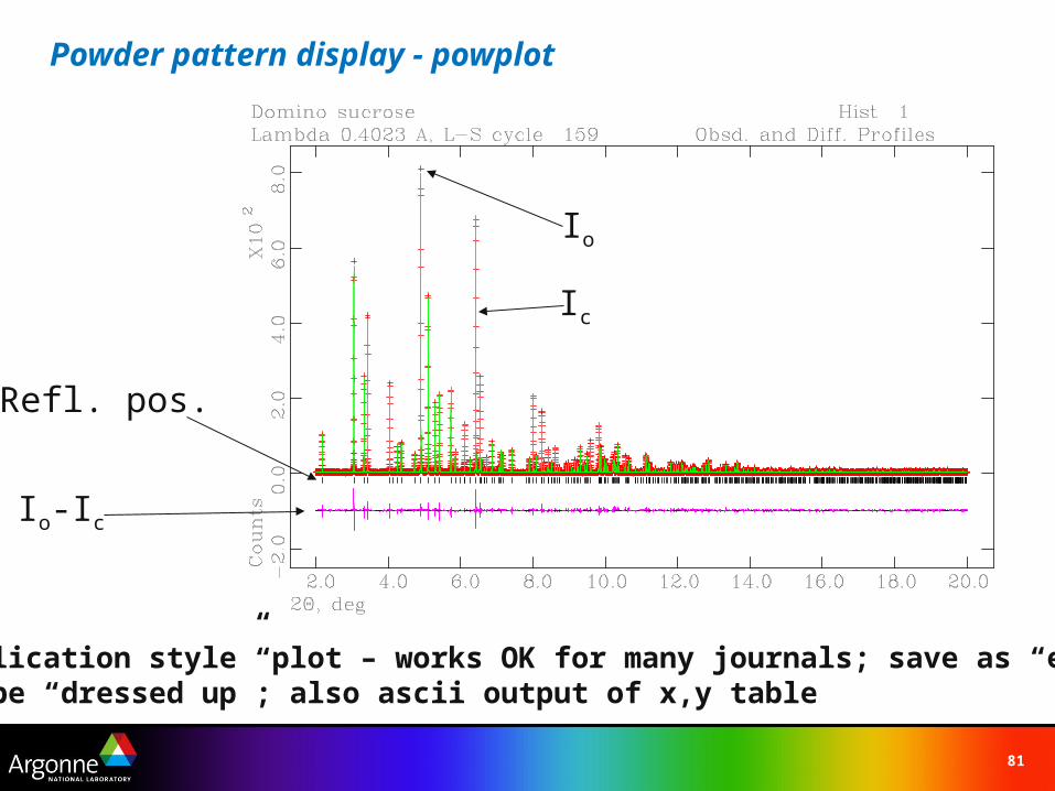
Powder pattern display - powplot
“publication style” plot – works OK for many journals; save as “emf”can be “dressed up”; also ascii output of x,y table
Io-Ic
Refl. pos.
Io
Ic
82
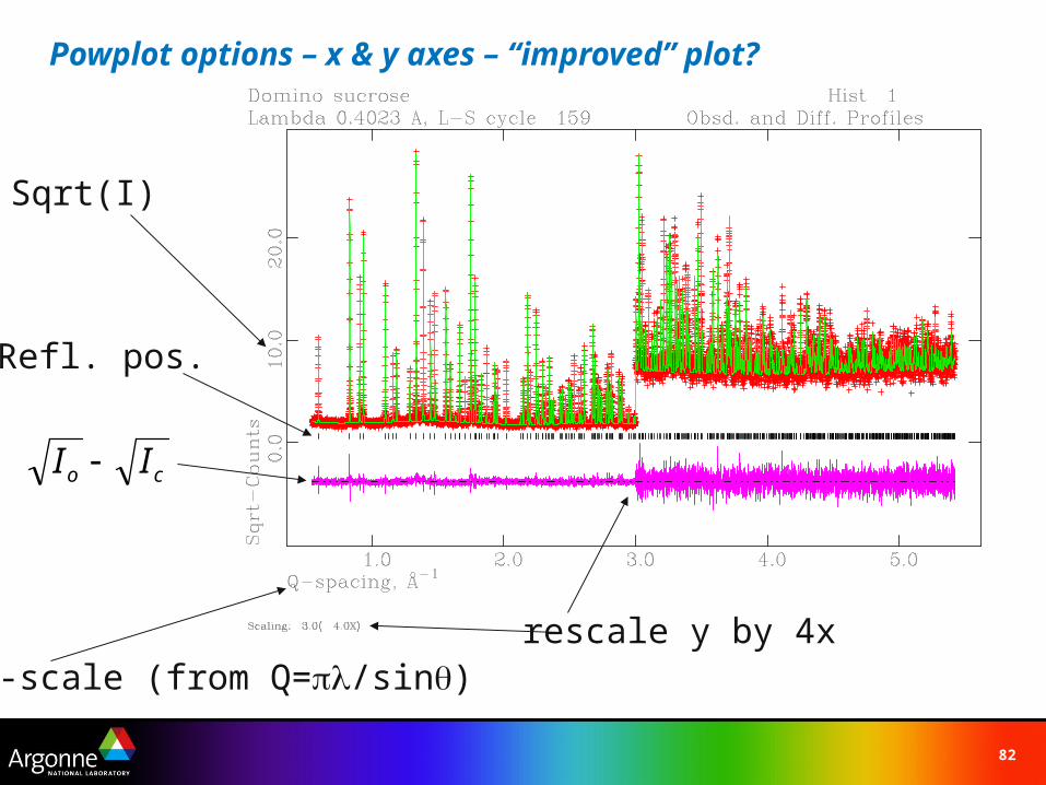
Powplot options – x & y axes – “improved” plot?
Sqrt(I)
Q-scale (from Q=/sin)rescale y by 4x
Refl. pos.
co II
83
Citations:
GSAS:
A.C. Larson and R.B. Von Dreele, General Structure Analysis System (GSAS), Los Alamos National Laboratory Report LAUR 86-748 (2004).
EXPGUI:
B. H. Toby, EXPGUI, a graphical user interface for GSAS, J. Appl. Cryst. 34, 210-213 (2001).