Embed Size (px)
Citation preview

Raytracing Dynamic Scenes on GPU
Thesis submitted in partial fulfillment
of the requirements for the degree of
Masters By Research
in
Computer Science and Engineering
by
Sashidhar Guntury
CVIT
International Institute of Information Technology
Hyderabad - 500 032, INDIA
May 2011

Copyright c© NAME, YEAR
All Rights Reserved

International Institute of Information Technology
Hyderabad, India
CERTIFICATE
It is certified that the work contained in this thesis, titled “Raytracing Dynamic Scenes on GPU” by
Sashidhar Guntury, has been carried out under my supervision and is not submitted elsewhere for a
degree.
Date Adviser: Prof. P. J. Narayanan

The world survives by those who have generosity of spirit.
But is owned by those who have none.
– Tarun J. Tejpal

Acknowledgments
The Bunny, Happy Buddha, Dragon are courtesy of the Stanford Scanning Repository. The Explod-
ing Dragon is courtesy of the UNC dynamic scene Benchmarks. The conference room was created by
Anat Grynberg and Greg Ward. Sibenik Cathedral was designed by Marko Dabrovic.
v

Abstract
Raytracing dynamic scenes at interactive rates to realtime rates has received a lot of attention re-
cently. In this dissertation, We present a few strategies for high performance ray tracing on an off-the-
shelf commodity GGraphics Processing Unit (GPU) traditionally used for accelerating gaming and other
graphics applications. We utilize the Grid datastructure for spatially arranging the triangles and raytrac-
ing efficiently. The construction of grids needs sorting, which is fast on todays GPUs. Through results
we demonstrate that the grid acceleration structure is competitive with other hierarchical acceleration
datastructures and can be considered as the datastructure of choice for dynamic scenes as per-frame
rebuilding is required. We advocate the use of appropriate data structures for each stage of raytracing,
resulting in multiple structure building per frame. A perspective grid built for the camera achieves per-
fect coherence for primary rays. A perspective grid built with respect to each light source provides the
best performance for shadow rays. We develop a model called Spherical light grids to handle lights
positioned inside the model space. However, since perspective grids are best suited for rays with a di-
rections, we resort back to uniform grids to trace arbitrarily directed reflection rays. Uniform grids are
best for reflection and refraction rays with little coherence. We proposean Enforced Coherence method
to bring coherence to them by rearranging the ray to voxel mapping using sorting. This gives the best
performance on GPUs with only user managed caches. We also propose asimple, Independent Voxel
Walk method, which performs best by taking advantage of the L1 and L2 caches on recent GPUs. We
achieve over 10 fps of total rendering on the Conference model with onelight source and one reflection
bounce, while rebuilding the data structure for each stage. Ideas presented here are likely to give high
performance on the future GPUs as well as other manycore architectures.
vi

Contents
Chapter Page
1 Introduction . . . . . . . . . . . . . . . . . . . . . . . . . . . . . . . . . . . . . . . . . . 11.1 Acceleration Datastructures . . . . . . . . . . . . . . . . . . . . . . . . . . . . .. . . 2
1.1.1 Kdtree . . . . . . . . . . . . . . . . . . . . . . . . . . . . . . . . . . . . . . 31.1.2 Bounding Volume Hierarchy . . . . . . . . . . . . . . . . . . . . . . . . . . 41.1.3 Grids . . . . . . . . . . . . . . . . . . . . . . . . . . . . . . . . . . . . . . . 5
1.2 Realtime Raytracing of Dynamic Scenes . . . . . . . . . . . . . . . . . . . . . . . .. 61.3 Realtime Raytracing and Our Contributions . . . . . . . . . . . . . . . . . . . . . .. 8
2 Background and Previous Work. . . . . . . . . . . . . . . . . . . . . . . . . . . . . . . . 102.1 GPU Computing Model . . . . . . . . . . . . . . . . . . . . . . . . . . . . . . . . . . 112.2 Acceleration Datastructure Construction . . . . . . . . . . . . . . . . . . . . .. . . . 122.3 Finding intersections through traversal of the datastructures . . . . . .. . . . . . . . . 14
3 Towards a Better Grid Datastructure. . . . . . . . . . . . . . . . . . . . . . . . . . . . . . 163.1 Indirect Mapping . . . . . . . . . . . . . . . . . . . . . . . . . . . . . . . . . . . .. 193.2 Culling of Triangles . . . . . . . . . . . . . . . . . . . . . . . . . . . . . . . . . . . .21
3.2.1 View Dependent Culling of Triangles . . . . . . . . . . . . . . . . . . . . . . 223.3 Results . . . . . . . . . . . . . . . . . . . . . . . . . . . . . . . . . . . . . . . . . . . 24
4 Bringing Coherence to Shadow Rays. . . . . . . . . . . . . . . . . . . . . . . . . . . . . . 264.1 Merging Shadow Rays . . . . . . . . . . . . . . . . . . . . . . . . . . . . . . . . .. 274.2 Rebuilding the datastructure for Shadow Rays . . . . . . . . . . . . . . . . .. . . . . 28
4.2.1 Mapping Shadow Rays . . . . . . . . . . . . . . . . . . . . . . . . . . . . . . 294.2.2 Reordering Shadow Rays . . . . . . . . . . . . . . . . . . . . . . . . . . . . .29
4.3 Load Balancing Shadow Rays . . . . . . . . . . . . . . . . . . . . . . . . . . . .. . 304.3.1 Hard and Soft Boundaries . . . . . . . . . . . . . . . . . . . . . . . . . . . .30
4.4 Spherical Grid Mapping . . . . . . . . . . . . . . . . . . . . . . . . . . . . . . . .. 324.5 Results . . . . . . . . . . . . . . . . . . . . . . . . . . . . . . . . . . . . . . . . . . . 34
5 Coherence in Reflection Rays. . . . . . . . . . . . . . . . . . . . . . . . . . . . . . . . . 395.1 Independent Voxel Walk (IVW) . . . . . . . . . . . . . . . . . . . . . . . . .. . . . 405.2 Enforced Coherence . . . . . . . . . . . . . . . . . . . . . . . . . . . . . . . .. . . . 415.3 Results . . . . . . . . . . . . . . . . . . . . . . . . . . . . . . . . . . . . . . . . . . . 43
6 Discussion and Conclusions. . . . . . . . . . . . . . . . . . . . . . . . . . . . . . . . . . 51
vii

viii CONTENTS
Bibliography . . . . . . . . . . . . . . . . . . . . . . . . . . . . . . . . . . . . . . . . . . . . 54

List of Figures
Figure Page
1.1 Raytracing illustrated (image courtesy wikipedia) . . . . . . . . . . . . . . . . .. . . 21.2 kdtree hierarchy from a set of points in space. . . . . . . . . . . . . . . .. . . . . . . 41.3 Building a BVH (image courtsey wikipedia) . . . . . . . . . . . . . . . . . . . . . .. 51.4 Spatial Subdivision using a regular grid . . . . . . . . . . . . . . . . . . . . .. . . . 61.5 Classification of different kinds of scenes encountered . . . . . . . .. . . . . . . . . . 7
3.1 Rays in the same tile move together and remain part of the same slab. . . . . . . .. . 163.2 Rays in the same tile move together and remain part of the same slab. . . . . . . .. . 193.3 Change in sorting time (smaller values are better) during datastructure building (left)
and average number of triangles checked (smaller values are better) during traversalstage (right) as number of threads in a block change. Larger number of threads implieslarger size of blocks. . . . . . . . . . . . . . . . . . . . . . . . . . . . . . . . . . . .20
3.4 256 x 256 imagespace tiles for sorting and DS building. The red colored tile representsthe size of the tile used for DS building. Four such tiles together form a greentile forraytracing, i.e., set of2 x 2 tiles are together handled in the raytracing step. . . . . . . 20
3.5 Heat map showing the number of triangles checked before declaring intersection. Leftimage corresponds to direct mapping while there is marked reduction in indirect map-ping (right). Number of triangles checked before declaring intersectionsincreases fromblue to pink and is highest in yellow regions. . . . . . . . . . . . . . . . . . . . . . .. 21
3.6 Plot demonstating the number of triangle-cell pairs in the DS building step. UniformGrid is constructed with all the triangles in the list. Perspective Grid is Built aftereliminating triangles using BFC and VFC. Also, using smaller cells, one reducestheduplication of triangles across cells. . . . . . . . . . . . . . . . . . . . . . . . . . .. 24
3.7 Example scenes – Happy Buddha, Conference, Fairy in Forest andSibenik Cathedral . 25
4.1 Reordering shadow rays results in distant but spatially close rays to behandled together. 284.2 Reordering illustrated. Different colors correspond to different cells. Sorting results in
all the same colors coming together.Get Boundariesgets the locations where enumer-ation of a new cell starts. Based on a therhold value (in this figure3), rays are dividedinto chunks and compacted in a tight array. . . . . . . . . . . . . . . . . . . . . . .. 31
4.3 Light outside the scene bounding all the triangles and light among the triangles and notbounding the model. . . . . . . . . . . . . . . . . . . . . . . . . . . . . . . . . . . . 33
4.4 Spherical space used for shadows. . . . . . . . . . . . . . . . . . . . . .. . . . . . . 334.5 Triangles included for shadow checking. . . . . . . . . . . . . . . . . . . .. . . . . . 344.6 Bounding rectangle of the geometry in spherical space defines the lightfrustum of interest. 35
ix

x LIST OF FIGURES
4.7 Time taken for rearrangement of shadow rays for shadow checking. . . . . . . . . . . 354.8 (a) Time taken for building perspective grid from point of view of light. Timings also
include time taken to compute spherical grid mapping and rearrangement of shadowrays for shadow checking. The plot also shows the times taken to construct a uniformgrid for the same scene. (b) Time taken by shadow rays to traverse the datastructure.UG is Uniform Grid [23], PG is our method and SBVH is Spatial BVHs [47]. . .. . . 36
4.9 Time taken as a function of distance of light from Fairy model. Times were taken forthe chunks of three different bin size – 64, 128 and 256. Timings were asnoted on GTX280. . . . . . . . . . . . . . . . . . . . . . . . . . . . . . . . . . . . . . . . . . . . . 37
4.10 Plot showing the number of lights required in a scene to let a per-frame built SBVH tobe faster than a per-frame per-pass built grid. Numbers are for HappyBuddha Model. . 38
5.1 The models and viewpoints used for evaluation of the performance of reflection rays.The models are Conference Room (284k), Happy Buddha (1.09M) andFairy Forest(174k). The Buddha model has the reflection parts coloured white. . . . .. . . . . . . 43
5.2 Percentage of rays declaring intersection at each step of iteration. Fairy grows veryslowly, taking 454 iterations to check reflections. In contrast, conference takes 306iterations. Happy Buddha takes just 294 iterations before declaring the status of thereflected rays. . . . . . . . . . . . . . . . . . . . . . . . . . . . . . . . . . . . . . . .44
5.3 Study of triangle and voxel distributions affecting reflection performance. Top left plotshows the concentration of rays in each voxel. Top right examines the tail of the plot.Longer tail with larger number of voxels is better for performance. Bottom left showsvoxel divergence in each tile. Bottom right examines the front. Higher number of tileswith less divergence is good for performance. . . . . . . . . . . . . . . . . .. . . . . 46
5.4 Comparison of traversal times between our method (Grid) and SBVH traversal (SBVH)[2] for various passes in a frame, viz. Primary, Shadow and Reflection rays. For shadowand secondary, time taken to rebuild the data structure and rearranging thedata is alsoincluded. Numbers are as noted on NVIDIA GTX 480. . . . . . . . . . . . . . .. . . 47
5.5 Plot showing the number of bounces required in a scene to let a per-frame built SBVHto be faster than a per-frame per-pass built grid. Numbers are for Happy Buddha Model. 48
5.6 In Fairy and Sibenik, only the floor is reflective. In case of Bunny floating in ConferenceRoom, the wooden table and the wooden frame of the red chairs is a highly polishedreflective surface. . . . . . . . . . . . . . . . . . . . . . . . . . . . . . . . . . . .. . 49
5.7 Dragon, Bunny collision in a conference room. . . . . . . . . . . . . . . . .. . . . . 50

List of Tables
Table Page
4.1 Time in milliseconds for primary and shadow rays for different stages for our methodand an implementation of Kalojanov et al. [23]. They use a uniform grid structure forprimary and shadow rays. Times are on a GTX480 GPU. . . . . . . . . . . . . .. . . 36
5.1 Time in milliseconds for reflection rays in each of the broadly classified stages. Thefourth column gives the number of ray-voxel pairs created during the enumeration ofrays and the fifth column gives the number of blocks assigned after compaction step.The last column gives the relative performance of the EC and IVW methods.. . . . . . 44
xi

Chapter 1
Introduction
Begin at the beginning and
go on till you come
to the end; then stop
– Lewis Carroll, Alice in Wonderland
For sometime now, raytracing has been the method of choice for producing photorealistic images.
Over the past few years, interactive to near realtime raytracing has slowlychanged from being out of
reach to being possible on a large scale computing setup and later even to a desktop with a commodity
graphics card in it. Interactive raytracing has slowly evolved to include more triangles, more lights and
more shading effects. This evolution has been due to the use of faster hardware and better algorithms
written to make optimum use of it.
The two methods of generating images in computer graphics, raytracing and rasterization have seen
a lot of development. raytracing is a technique that generates an image of a scene by simulating light
travel in the real world. In real world, light rays are emitted from the light source and illuminate the
scene. These rays depending on the object they strike, reflects off orpass through them. These rays hit
our eyes or in the case of computer graphics, the synthetic lens. Becausea vast number of rays never
hit the lens, the simulation of this phenomenon is done backwards, i.e, rays are generated from the lens
which hit objects (figure 1.1). For every pixel in the image, one or more rays is shot to see if it intersects
an object. Everytime there is a hit, color is calculated using the light position. More rays might be
generated at this point for reflection and refraction which adds to the realism of the scene.
Rasterization on the other hand is a technique used for determining the objectsthat are visible to the
camera. It does not tell us the appearance of objects with respect to each other in a scene. For this reason,
rasterization by itself can not handle effects like reflection, refraction, shadows, etc. However there are
techniques (at extra cost of computing) like stencil buffer and shadow mapping which overcome some
of the issues and handle the aforementioned effects. Dedicated GraphicsProcessing Units (GPUs)
accelerate the process of rasterization because of which rasterization isa fast process but each and every
step adds an overhead eventually causing the system to significantly slow down.
1

Figure 1.1Raytracing illustrated (image courtesy wikipedia)
Both techniques are used in the movie industry where time to render is not a constraint. However,
in the gaming industry, only rasterization is used because they need interactive performance. There are
dedicated GPUs for the purpose of the accelerating the process. However, as games begin to demand
more realism and raytracing becoming more interactive, hybrid games with a mix of rasterization and
raytracing might come out.
Algorithm 1 Basic raytracing algorithm
for each pixel in the imagedocompute viewing rayfind first object hit by ray and get the normalset the pixel color according to material, light position and normal
end for
Algorithm 1 illustrates simple raytracing which computes the pixel colors in the resultant rendered
image using the data of the first intersections. In order to get the object which is first hit by the ray, one
has to test the ray against all the objects in the scene and get the first hit. Asthe complexity of the scene
increases, the number of objects in the scene increases. In a typical gamescene of about 10 million
triangles and a typical movie shot with more than a billion triangles, this method is bound to take a very
long time to get the hit objects. However, this problem can be solved using the fact that rays travel in a
straight line and we need to check the ray against only those objects which are either in the path or near
the path of the ray. To do this, often spatial datastructures called Acceleration Datastructures are used
which can spatially arrange the objects such that ray by the virtue of its direction can query only those
objects which are in the path of its travel.
1.1 Acceleration Datastructures
The process of raytracing can be markedly speeded up by utilizingAcceleration Datastructures
(AD) like Kd-trees, grids and Bounding Volume Hierarchies (BVH). These structures exploit the fact
2

that rays in a scene are not random or arbitrary in nature. Often groups of rays agree with the direction
in which they move. This is calledspatial coherence. Spatial Coherence is particularly high for rays
like camera rays and shadow rays. Coherence allows combining severalrays together in a packet or
a frustum and tracing these bundles of rays. These bundles of rays are then traversed through an AD.
Depending on the kind of the acceleration datastructure used, coherence may or may not be exploited.
Finding an intersection for a ray in a scene is often treated as a search problem. Search is made faster
by enforcing some order among the elements, often by sorting. Accelerationdatstructures use this to
speedup raytracing. Treating rays as part of a packet helps us treatthem together both at a logical level
and as well as the programmatical level when we use SIMD architectures to process the rays in parallel.
These packets allow data to be brought in at once which helps in removing bottlenecks involved in
getting costly data transfers. Choosing the right AD is very important and is done keeping in mind
various factors. For the past few years, the most important aspect hasbeen traversal performance [17].
Traversal depends on whether we use spatial subdivision or object hierarchy. In spatial subdivision,
we divide the whole world into separate entities, each encompassing a different number of triangles.
Each triangle can belong to one or more subdivisions. In contrast, objecthierarchy references triangles
multiple times in often overlapping entities. In space subdivision structures, each entity is represented
only once and so the traversal algorithm can traverse these entities in front-to-back order and termi-
nate when they find an intersection. Object hierarchy techniques, on the other hand, rely on visiting all
the entities along the the path of the ray irrespective of finding intersection. However, since there is a
hierarchy, in the end, every triangle is checked only once in the leaf nodes. This leads to fewer intersec-
tion tests but at the cost of devoting more time in building such a hierarchy. There are various aspects
across which we can compare ADs. We concentrate on build time and build quality. In this thesis, we
assume axis aligned bounding boxes (AABB) that are non-adaptive. Build time and build quality are
two opposing factors and concentrating on one leads to the deterioration ofthe other. There are various
algorithms to estimate the the quality of the AD built. The most well known is the class ofSurface Area
Heuristic (SAH) algorithm [14, 17]. These algorithms significantly increasethe time needed to build
the datastructure. We now briefly describe the three most popular acceleration datastructures.
1.1.1 Kdtree
Among the spatial datastructures, kdtrees are very efficent for traversal and finding the right triangle
for intersection, making it the fastest datastructure for accelerating pureraytracing performance. Be-
cause of the hierarchy, traversal to the leaf node is cheap and efficient as a large number of triangles
are eliminated reducing the number of intersection tests. The efficiency of traversal depends on the
quality of the datastructure which in turn depends on how well it treats different kinds of rays arriving
in arbitrary directions. This metric is accomodated in the datastructure using a greedy technique called
Surface Area Heuristic (SAH) [14]. These methods provide the means to estimating the cost of traversal
based on the distribution of the rays in the scene.
3

First we assume a uniformly distributed set of rays, for whom, the probabilityPhit of hitting a vol-
umeV is proportional to the surface area SA of that volume. If inside the volumeV , the probability of
hitting a sub-volumeVsub is
Phit(Vsub|V ) =SA(Vsub)
SA(V )
For a random ray R, the cost of testing intersection against a node N isCR. CR is the sum of the
traversal stepKT and the sum of the expected intersection costs of its two children, weighted bythe
probablity of hitting them. The intersection cost of a child is locally approximated tobe the number of
triangles contained in it times the costKt to intersect one triangle. If the two child nodes of NodeN are
Nr andNl, each havingnr andnl triangles in them, then expected cost can be computed as
CR = KT + Kt[nlPhit(Nl|N) + nrPhit(Nr|N)]
l5
l 2
l 8
l 4
l 9
l 1l 7
3l
l 6
p4 p
10
p2
p1
p3
p7 p
8
p6
p9
p5
Figure 1.2kdtree hierarchy from a set of points in space.
In the recursive build of a kdtree, one needs to break a node into two subnodes. This decision is
made on the basis of SAH, where split is made at point which gives the minimal possibleCR. If the cost
of splitting is higher than the already determinedCR, then the node is left as a leaf node. To compute
the split planes efficiently, many algorithms have been proposed some of themhave been described in
[14, 28, 51]
1.1.2 Bounding Volume Hierarchy
Bounding Volume Hierarchy is a hierarchy over the geometric objects in the scene. Every object
in the scene is enclosed in a tight bounding volume giving a set of bounding volumes. Some of these
4

volumes together can be enclosed in a tight bounding volume obeying some heuristic such as a volume
can not be larger than a preset dimension or the sum of the volumes combinedshould be minimal. Like
kdtrees, these heuristics are captured in a greedy technique called Surface Area Heuristic (SAH). As we
move from bottom to top, the volume encompassed by the volumes increases with the root node having
the entire scene. Thus when rays need to compute intersection, they checkagainst the node and descend
to the child nodes only if they pass through the bounding volume. For this reason, it is important to have
a simple bounding volume which can be tested against the ray very fast.
Figure 1.3Building a BVH (image courtsey wikipedia)
On one hand, a simple bounding box keeps the intersection test simple and fast. On the other hand,
the bounding box must be able to fit the objects in its volume as tightly as possible. Often, an axis
aligned bounding box (AABB) bounding volume is used. Often, long triangles are also split over two
or more volumes to get a tight bounding box. Bounding box at each level needs a few bytes to store
information and can be checked very efficiently. BVHs were introduced primarily to solve the issues
posed by kdtree. With their efficient traversal times, kdtrees were well suited for static scenes as their
build time is very high. With small changes in the geometry, a kdtree is invalidated. BVHs with a kdtree
like hierarchy and a faster build process are better suited for dynamic scenes. Incrementally updating the
BVH involves checking the volumme where the changes took place and updating them appropriately.
Though it has been seen that with every update, the quality of the tree decreases. Therefore, techniques
have been proposed to check if the quality is below a certain threshold to go for a complete rebuild of
the hierarchy. BVHs, due to their efficient elimination of geometry are used extensively in games for
collision testing [12, 26]. In most respects like memory consumption, traversal techniques, ability to be
parallelized, and frusta suitability, BVH methods come close to kd-trees. In addition, they are faster to
build and easier to update.
1.1.3 Grids
While BVH and Kd-trees are hierarchical datastructures, grids fall into the category of uniform
spatial subdivision. The datastructure does not adapt to the complexity ofthe scene though there has
been some work towards this [22]. Adaptive structures handle complex geometry but are harder to
build and even harder to update. However, grids are very fast to build and therefore rebuilding a grid
datastructure maybe more attractive than updating the datastructure.
5

Figure 1.4Spatial Subdivision using a regular grid
Grids work by binning triangles into spatial cells. Conceptually it is similar to radixsort and can be
looked as a rasterization of triangles into coarse cells. The best part about grid datastructure is that it
can be built in a single pass. There are various parallel techniques whichmake it very fast. A complete
rebuild of a grid is usually faster than refitting a BVH to reflect the changes ina dynamic scene. Being
able to rebuild every frame, one does not have to make any assumption about the motion which makes
grids an attractive option for fully dynamic scenes. However, grids lose out in traversal performance due
to lack of hierarchy. Since, the space is uniformly divided, rays as packets attain little advantage. Often
rays are treated independently and if divergence among rays is high, traversal is affected significantly.
However, some techniques like mailboxing and slicewise coherent traversal allow us to use the natural
coherence which might be present and exploit the SIMD hardware to getbetter performance.
1.2 Realtime Raytracing of Dynamic Scenes
A good quality datastructure can reduce the traversal times. Parallelizing thetraversal and using
the features of the architecture can take the performance further up. But the most compelling question
during the design of a realtime raytracer for dynamic scenes is how to build, rebuild or update the
AD to reflect the changes. As mentioned, build quality can result in substantial improvements in ray
traversal performance but at the cost of more time spent on building sucha datastructure. Almost
realtime raytracers need to be able to build a good datastructure fast and beable to traverse it quickly.
There are several factors which can impact this decision [51]. To decide on the time-quality tradeoff,
one has to inspect one or more of the following –
• Motion of different kinds . Having a scene that is static, i.e., where triangles do not move,
devoting significant time to build a good quality datastructure is worthwhile as the scene will
not change and the high cost of building the hierarchy would be amortized during speedy ray
traversal.
6

• Total number of rays. All things remanining equal, if more rays are being traced, it may be
worthwhile to spend more time on building such that rays collectively will better exploit coher-
ence. Also, sampling and multiresolution techniques demand more rays which can increase the
ray count.
• Kind of rays and number of passes. Secondary rays, especially the ones for reflection, area
lights, etc., may access ADs in a haphazard manner affecting the performance. If multiple passes
are required, many kinds of incoherent rays may be present, which hasthe potential of slowing
down the system if traversal is inefficient. Different kinds of rays havediffering properties and
one kind of AD might not be suitable for the other. Therfore rays based on their type and their
behavior need to use different AD or one that adapts well across different kinds of rays.
With respect to the above points and the discussion on various ADs, grid is fastest to build but
inefficient to traverse. Kd-trees are on the other hand very costly to buildbut efficient to traverse. BVH
lies in the middle of the spectrum. Often, the design decisions of which acceleration structure to use
is driven by these considerations. Scenes can be divided into various categories as shown in figure 1.5.
For dynamic scenes, one has to build the datastructure from scratch or update it to reflect changes in
geometry. This can be done by flagging parts of the scene which have changed and then redistributing
them in the scene appropriately. In case of animated scenes, knowing the motion can be explored to
speedup the rebuilding part of the scene.
Figure 1.5Classification of different kinds of scenes encountered
We explore a general scenario where changes are not known and therefore rebuilding the datastruc-
ture or updating it are the only ways possible. Previous work by Patidar and Narayanan [38] concen-
trated on rebuilding the grid datastructure from scratch for every frame.We take this idea forward
by extending it to updating the datastructure in the conclusion section. Rebuilding the datastructure
depends a lot on the kind of datastructure and the time it takes to get constructed.
7

1.3 Realtime Raytracing and Our Contributions
Parallelization is at the heart of realtime raytracing. Raytracing is an inherently parallel application
as the color of each pixel in the resultant image is independent of other. Also at the datastructure
building level, a lot of observations have been made leading to more efficientdatastructure building
techniques. There has been a lot of work on speeding up raytracing onthe CPU and using the SIMD
instructions of CPU to parallelize ray traversal. This is often attained by optimizing the codes for the
hardware. Knowledge of the underlying hardware often yields substantial speedup. With advances in
parallel computing and architectures, speedup through hardware is bound to increase at a steady rate.
GPU based computing has recieved a lot of attention in the high performance computing sphere
due their high computation power packed in affordable and easily available hardware. Raytracing is
a massively multithreaded application which has the potential of using the GPU architecture to get
significant speedup. GPU based raytracing has seen action both in datastructure building as well as
traversing the rays. However, there has been very little study in the issue of raytracing for truly dynamic
scenes. As mentioned earlier, to raytrace dynamic scenes, one has to be able to build the datastructure
very fast. To this end, some of the contributions made in this work are
• Modified the grid datastructure of our previous work to eliminate triangles thatdo not contribute
to raytracing.
• Introduced a technique of indirect mapping to exploit faster sorting and atthe same time higher
SIMD width.
While coherent and locally coherent rays benefit from the datastructures with hierarchies, grid based
datastructures do not enjoy the benefits of coherence and packets. This is especially important in the
context of realtime raytracing as coherence at every level needs to be exploited to make the system
faster. We look at shadow rays and propose the following ideas to improveperformance of shadow rays
• Fast shadow tracing by extending perspective grids to shadow rays
• Used spherical grid mapping to accomodate lights inside a scene.
• Load balancing to distribute unevenly spread shadow rays evenly for better processing.
We also look at true secondary rays which are not coherent and take reflection rays as an example of
these kinds of rays. The behavior of seondary rays is often dependent on kind of the scene and we take
a few models representative of their kind and try to understand the traversal of reflection rays. For this
• Proposed Enforced Coherence (EC) method to gather rays and treat them together.
• Modified the load balancing scheme of shadow rays to achieve equitable distribution for process-
ing.
8

• Compared EC with a more classical technique like Independent Voxel Walk (IVW) on two gen-
erations of graphics hardware to note the performance changes.
Broadly speaking, our message is to look at raytracing in different stages. We try to build appropriate
datastructures for each stage to aggresively save on timings and keep thetraversal times low. We also
try to reduce the overall time consumed for each frame to achieve near realtimeraytracing of scenes
with arbitrarily changing geometry.
9
Chapter 2
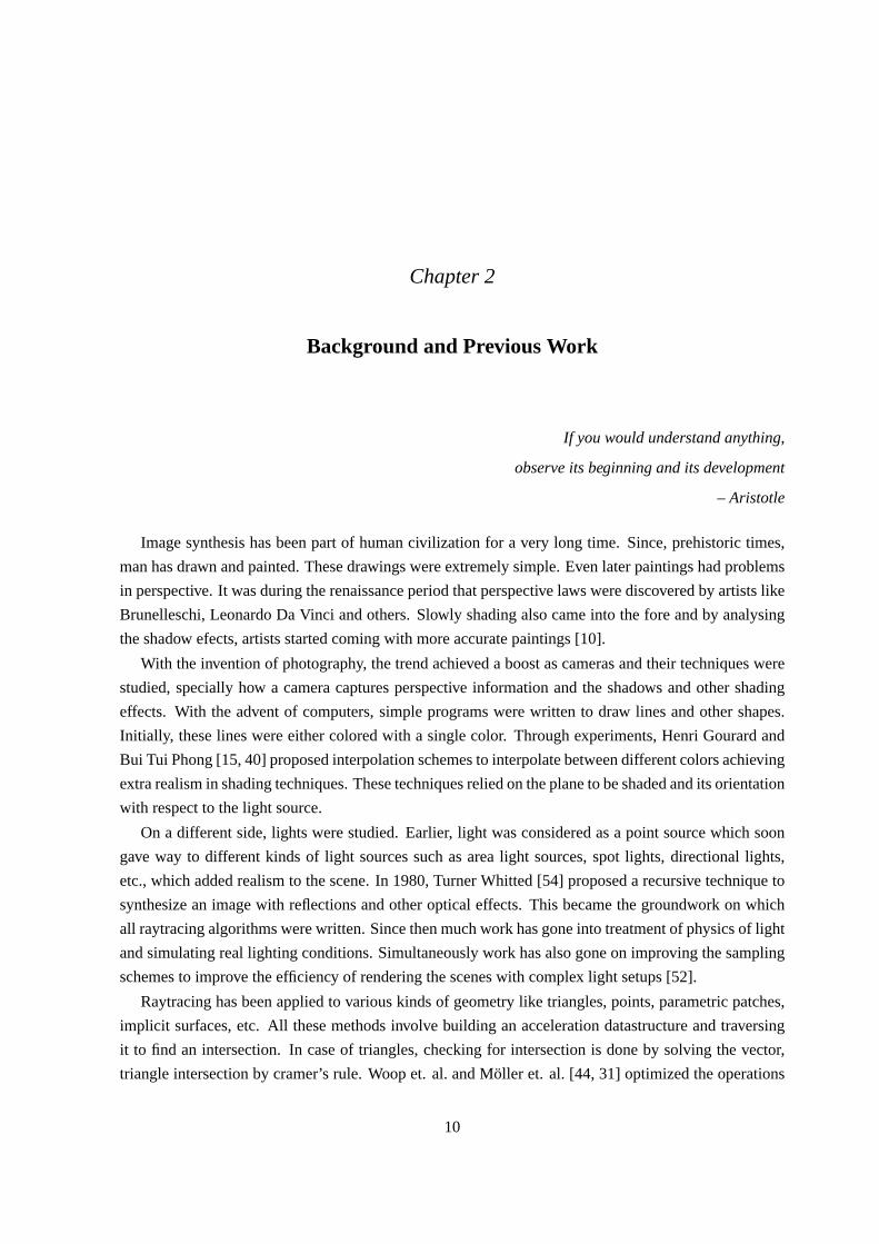
Background and Previous Work
If you would understand anything,
observe its beginning and its development
– Aristotle
Image synthesis has been part of human civilization for a very long time. Since, prehistoric times,
man has drawn and painted. These drawings were extremely simple. Even later paintings had problems
in perspective. It was during the renaissance period that perspective laws were discovered by artists like
Brunelleschi, Leonardo Da Vinci and others. Slowly shading also came intothe fore and by analysing
the shadow efects, artists started coming with more accurate paintings [10].
With the invention of photography, the trend achieved a boost as cameras and their techniques were
studied, specially how a camera captures perspective information and the shadows and other shading
effects. With the advent of computers, simple programs were written to draw lines and other shapes.
Initially, these lines were either colored with a single color. Through experiments, Henri Gourard and
Bui Tui Phong [15, 40] proposed interpolation schemes to interpolate between different colors achieving
extra realism in shading techniques. These techniques relied on the plane tobe shaded and its orientation
with respect to the light source.
On a different side, lights were studied. Earlier, light was considered asa point source which soon
gave way to different kinds of light sources such as area light sources, spot lights, directional lights,
etc., which added realism to the scene. In 1980, Turner Whitted [54] proposed a recursive technique to
synthesize an image with reflections and other optical effects. This became the groundwork on which
all raytracing algorithms were written. Since then much work has gone into treatment of physics of light
and simulating real lighting conditions. Simultaneously work has also gone on improving the sampling
schemes to improve the efficiency of rendering the scenes with complex light setups [52].
Raytracing has been applied to various kinds of geometry like triangles, points, parametric patches,
implicit surfaces, etc. All these methods involve building an acceleration datastructure and traversing
it to find an intersection. In case of triangles, checking for intersection is done by solving the vector,
triangle intersection by cramer’s rule. Woop et. al. and Moller et. al. [44, 31] optimized the operations
10

on hardware bringing raytracing closer to interactive rates on commodity hardware. For parametric
patches, methods are either subdivision based or numerical based. Subdivision techniques have various
traversal steps before subdividing the bounding volume patch. Numerical techniques invovle solving
an equation which might involve high complexity. In case of many models, it is notuncommon to see
primitives with 18 degree equations. Starting with Kajiya et. al. [21] which solved a 18 degree univariate
polynomial, several other techniques were also proposed like Toth et. al. [48] using multivariate Newton
iteration. Manocha and Krishnan [29] used Eigenvalue methods to do the same.
Point based rendering was proposed first by Levoy and Whitted [16] by arguing that points are pow-
erful enough to model any kind of object and details which scanline rendering often lose. Reyes archi-
tecture [8] was a step in the similar direction albeit breaking the scene into micropolygons. Rusinkiewicz
and Levoy later devised datastructures for hierarchical culling and LOD. There has been a lot of work
in sampling the model to produce point samples like randomized sampling Wand et. al. [53] or deter-
ministic sampling of Stamminger and Drettakis [46].
Implicit and procedurally generated surfaces have played a crucial role in computer graphics. They
do not have detail issues like polygonal geometry and can be tesselated based on LOD factors. Tradi-
tionally polygonalization has been used to convert implicit surfaces into triangulated models [6] before
rendering it. Marching Cubes algorithm can create polygonal models fromimplicit surfaces. Purcell et.
al. [42] and Loop and Blinn [27] demonstrated raytracing of quadratic and cubic-spline curves on the
GPU.
2.1 GPU Computing Model
GPU based methods have been used extensively to speed up applications with massive paralellism.
GPUs offer finegrained parallelism along with wider SIMD width which allows larger number of threads
to process same intruction together. This is especially useful in graphics, vision and scientific computing
problems where there the instructions are same and data is different and instruction divergence is less.
Programs which utilize the GPU are typically written in CUDA [34] though they canbe written in other
ways like OpenCL and Direct Compute as well. These enviroments provide anabstract layer of blocks
and threads which hides the internal architecture of the GPU and lets the programmer write programs
which scale with changing number of cores in the GPU. These programs consist of CPU code which
can invoke upwards of thousands of instances of code to be run on GPUusing hardware threads. These
large number of threads are logically organised in groups called blocks. Threads within a single block
have the advantage of cooperating with each other and can be synchronized with negligible overhead.
They also share data on a small yet high speed on chip shared memory. On newer architectures, these
threads have access to an L1 cache. Threads across blocks share data on a slightly slower L2 cache and
a much slower but considerably larger global memory.
During the execution of the GPU code (kernel), threads are scheduled inbatches of 32 (warp) which
are then launched. These 32 threads execute the same instruction but on different data. Often codes have
11

branching instructions which cause the batch of 32 threads to break into chunks of threads for different
routes of divergence. Each of the these chunks are processed sequentially. Therefore, it is desirable to
have as few branching instructions with divergence as possible. Also, memory access patterns affect
the performance deeply. Threads tend to favourcoherent accesseswhere spatially close locations in
memory are accessed. This is because when a thread accesses a locationin memory, it retrieves a 188
bit chunk of that memory making other accesses amortized. Access time becomes higher when far away
locations are accessed simultaneously by threads of the same warp. Additionally, threads would want
their data to be in fast on chip locations due to which it is best to get data from slow global memory to
fast shared memory and use it from there.
Like all prallel programs, programs written in GPU often borrow ideas of efficiently collecting data,
data movement, data sorting and data rearrangement [5]. Sengupta et al. [45], Patidar et al. [37], Satish
et al. [43] proposed various efficient implementations of these ideas whichare popularly called as primi-
tives. A sort primitive takes an array and outputs the sorted version of it. There are many more primitives
which we constantly used to in our methods. GPU based computing methods havebeen used extensively
in areas like protein folding, fluid simulation, stock options simulations etc., [35] totake advantage of
the fine grained parallelism and attain orders of improvement over single core implementations.
2.2 Acceleration Datastructure Construction
Raytracing used to be a slow offline process traditionally but has entered the realm of interactive
graphics and is used widely now. With proliferation of high performance hardware at commodity prices,
raytracing performance is pushed upwards continously. These speedups have been due to (a) advance-
ments in the algorithm and datastructure sphere and (b) using better hardware and writing optimized
code for the particular hardware. Wald et al. [51] surveyed many of thecurrent techniques in raytrac-
ing which over the years have translated to performance improvements in raytracing using multicore
architectures. Here we describe some of the recent work which is directlyrelated to our own.
The datastructure building part of raytracing has often been looked as apreprocessing step and not
considered part of the actual raytracing With raytracing becoming interactive, applications can not as-
sume that the scenes to be rendered have static geometry. In truly generalcases, there may be objects
flying, colliding, breaking, etc. This change in geometry invalidates the spatial datastructure built previ-
ously. For correctness reasons, datastructure has to be built repeatedly. This can become the bottleneck
in the process of raytracing. However, much effort has gone into speeding up the process of building
these datsatructures. On the GPU front, Zhou et al. [55] gave efficientparallel methods for constructing
kdtrees on GPU. While they were efficient in terms of speed, they consumeda lot of memory which re-
stricted their usage to small to moderately sized scenes (upto 600k triangles).Hou et al. [18] exteneded
this method using better memory allocation strategies accounted for this problem and made kdtress suit-
able for very large models (more than 7.5M triangles) as well. The methods we propose are valid for
moderate to large models with emphasis on speed and interactivity. While the kdtrees generated using
12

the methods offer interactive to almost realtime performance for raytracing,their kdtree building time
is still high effectively making the entire process slow if the datastructure needs to be built constantly.
BVH has also been studied widely in recent times due to its relatively lower construction times.
Compared to kdtrees, BVHs have lower memory footprint. Classic methods do not split triangles keep-
ing the memory usage constant. Also, since primitives are referenced only once, the construction time
is relatively fast. Ajmera et al. [3] and Wald et al. [49] gave fast methods tocreate hierarchies which
were extended by Lauterbach et al. [25] to give better building methods. These methods can build the
datastructure fast [36] but lose out on the quality benchmark making the traversal time higher. Methods
like splitting triangles were proposed in [11, 9, 47]. Splitting triangles was considered a kdtree tech-
nique and using it in BVH improved the overall quality of the hierarchy but significantly increased the
building time. Moreover, these techniques are considerably serial and efficient methods to build them
on GPU is still an issue. There has also been research on enforcing space subdivision to build optimal
BVHs by Popov et. al. [41]. Their method proposes a space partitioning algorithm to build a better
BVH. Again this technique improves the quality of BVH but takes higher time in building the hierarchy.
In contrast to BVH and kdtree methods, grids have recieved less attentions. BVH and kdtree are
algorithmically superior datastructures for traversal due to the inherent hierarchy making it possible to
eliminate a large number of triangles cheaply. However, due to the simplicity of thegrid construction,
several methods were proposed to construct it efficiently on CPU. Ize et al. [20] and Lagae and Dutre
[24] gave heuristics to measure the quality of the grid and ability to improve it. However, these tech-
niques led to little performance improvements. However, they were still faster than BVH or kdtree for
construction. On the GPU front, Patidar and Narayanan [38] gave a fast method to sort the triangles and
construct a grid datastructure. However, this datastructure building process was dependent on atomic
operations. If triangle distribution was high in some region, atomic operations could significantly de-
crease the performance of the datastructure building. This problem was solved later by Kalajanov and
Slusallek [23] on the newer hardware by sorting on triangle-cell pairs. Their method differed in the way
that they created a list of triangles falling in each cell of grid and sorted the triangle-cell pairs based on
the cell values thus getting a list of triangles for each cell. Grids are different from BVH and kdtree
because they do not adapt to the complexity of the scene. Often the entire scene is uniformly divided
into cells, some of which maybe sparsely populated while others have a lot of triangles. This situation
is often calledteapot in a stadiumscenario where in a grid spanning a large stadium have sparse grid
cells everywhere, except for a few cells with dense population of triangles. This scenario leads to higher
datastructure building times as the number of triangles in the same cell is quite largeand binning them
into the same location would result in higher times. Our method which is grids is based on the princi-
ples proposed by Patidar and Narayanan [38] but we borrow the grid building ideas from Kalojanov and
Slusallek [23] to make our grid building more robust to scenes.
13
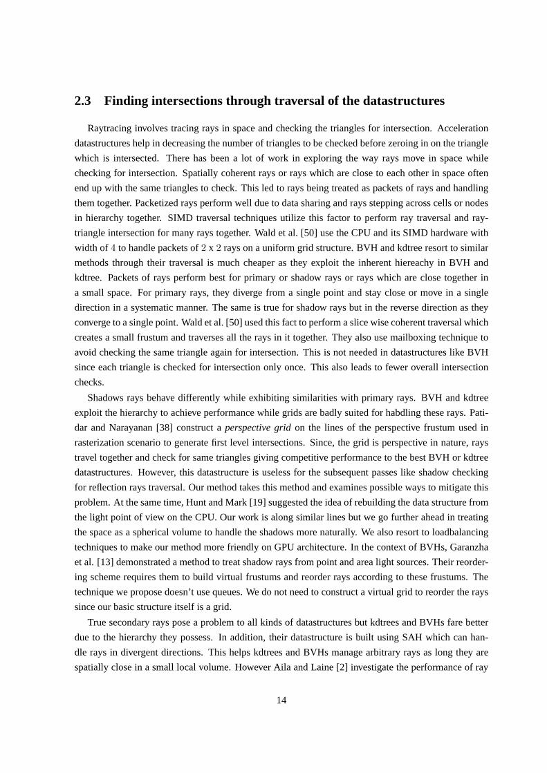
2.3 Finding intersections through traversal of the datastructures
Raytracing involves tracing rays in space and checking the triangles for intersection. Acceleration
datastructures help in decreasing the number of triangles to be checked before zeroing in on the triangle
which is intersected. There has been a lot of work in exploring the way rays move in space while
checking for intersection. Spatially coherent rays or rays which are close to each other in space often
end up with the same triangles to check. This led to rays being treated as packets of rays and handling
them together. Packetized rays perform well due to data sharing and rays stepping across cells or nodes
in hierarchy together. SIMD traversal techniques utilize this factor to perform ray traversal and ray-
triangle intersection for many rays together. Wald et al. [50] use the CPU and its SIMD hardware with
width of 4 to handle packets of2 x 2 rays on a uniform grid structure. BVH and kdtree resort to similar
methods through their traversal is much cheaper as they exploit the inherent hiereachy in BVH and
kdtree. Packets of rays perform best for primary or shadow rays orrays which are close together in
a small space. For primary rays, they diverge from a single point and stay close or move in a single
direction in a systematic manner. The same is true for shadow rays but in the reverse direction as they
converge to a single point. Wald et al. [50] used this fact to perform a slicewise coherent traversal which
creates a small frustum and traverses all the rays in it together. They alsouse mailboxing technique to
avoid checking the same triangle again for intersection. This is not needed indatastructures like BVH
since each triangle is checked for intersection only once. This also leads tofewer overall intersection
checks.
Shadows rays behave differently while exhibiting similarities with primary rays.BVH and kdtree
exploit the hierarchy to achieve performance while grids are badly suited for habdling these rays. Pati-
dar and Narayanan [38] construct aperspective gridon the lines of the perspective frustum used in
rasterization scenario to generate first level intersections. Since, the grid is perspective in nature, rays
travel together and check for same triangles giving competitive performance to the best BVH or kdtree
datastructures. However, this datastructure is useless for the subsequent passes like shadow checking
for reflection rays traversal. Our method takes this method and examines possible ways to mitigate this
problem. At the same time, Hunt and Mark [19] suggested the idea of rebuilding the data structure from
the light point of view on the CPU. Our work is along similar lines but we go further ahead in treating
the space as a spherical volume to handle the shadows more naturally. We also resort to loadbalancing
techniques to make our method more friendly on GPU architecture. In the context of BVHs, Garanzha
et al. [13] demonstrated a method to treat shadow rays from point and area light sources. Their reorder-
ing scheme requires them to build virtual frustums and reorder rays according to these frustums. The
technique we propose doesn’t use queues. We do not need to construct a virtual grid to reorder the rays
since our basic structure itself is a grid.
True secondary rays pose a problem to all kinds of datastructures butkdtrees and BVHs fare better
due to the hierarchy they possess. In addition, their datastructure is built using SAH which can han-
dle rays in divergent directions. This helps kdtrees and BVHs manage arbitrary rays as long they are
spatially close in a small local volume. However Aila and Laine [2] investigate theperformance of ray
14

traversal in a true general case. They schedule rays in a persistent fashion to accomodate for the small
ray divergence to get better performance. Their results depend on thequality of the datastructure which
in turn depends on the amount of time invested in building it. There has been somework on enforcing
coherence among secondary rays. Pharr et al. [39] and Navratil etal. [33] proposed reordering tech-
niques on multicore CPUs. The ray reordering technique proposed by Pharr et al. [39] queues rays
and schedules the processing of this queue in a way to minimize cache misses and I/O operations. Re-
cently, Moon et al. [32] suggested the use of Hit Point Heuristic and Z-curve filling based ray reordering
to achieve cache oblivious coherence on multicore architectures. They concentrate on simplifying the
model and using these simplified models for global illumination methods such as pathtracing and pho-
ton mapping. There has been some work on secondary rays on the GPUs.Budge et al. [7] analyzed the
bottlenecks during pathtracing a complex scene and proposed a softwaresystem that splits up tasks and
schedules them appropriately among CPU and GPU cores. Our method usesprimary hit points from ray
casting for reordering the rays. Aila et al. [1] proposed possible extensions to hardware which can speed
up secondary rays. Their treatment is from a hardware point of view studying the cache performance.
We concentrate on speeding up the tracing of reflection rays.
15

Chapter 3
Towards a Better Grid Datastructure
The ability to simplify means
to eliminate the unnecessary so that
the necessary may speak.
– Hans Hoffman, Search for the Real
Motivated by our need to raytrace moderately large scenes (upto 2M triangles) at interactive to near
realtime rates, we propose building a grid datastructure. Grid datastructureis cheap to build and can
be tailor made easily for a particular kind of rays. Our grid datastructure building carries forward the
technique proposed by Patidar and Narayanan [38] where we create athree dimensional datastructure
with two dimensionaltiles in image space and slabs in the depth direction (much like in rasterization)
of the camera. The resultant volume of space bounded by the tile dimensions and by a finite depth is a
cell.
Figure 3.1Rays in the same tile move together and remain part of the same slab.
The result of the raytracing is an image, whose each pixel value is the result of its corresponding
ray’s intersection. In their work, Patidar and Narayanan [38] divide this image into tiles and all the rays
16

in a tile are coupled together. It should be observed that rays when diverging from a camera position
move out in a frustum. These rays hit the image grid and fall into their respective tiles. These tiles are
of finite depth, calledslabsand extend in the direction of rays. If the size of slabs grows at the same
size as the divergence of the rays, all the rays which were part of a tile will always be part of the same
slab at all times.
In their implementation, Patidar and Narayanan [38] divide the space along the direction of camera
into discrete slabs. First, they determine to which tile each triangle belongs. Thisis determined by
finding theX andY bounds of triangle in the image space. Using three passes, each sorting thetriangles
alongX, Y andZ dimensions respectively, a list is obtained where triangles are clustered based on the
cell they fall in. TheX, Y andZ are concatened into a single unsigned integer and hierarchically sorted
to obtain the ordering. A final scan pass gave the number of triangles in each cell. All this sorting was
done based on theX, Y bounds and the nearestZ slab value. Therefore resolution of the grid played
an important role in making a good quality datastructure. A finer grid would meanfiner sorting and
better binning of triangles but at the cost of extra time spent in sorting. Aftermany experiments, they
concluded that128 x 128 x 16 was a resolution where the time required to sort and the quality of the
grid datastructure struck an optimal balance.
One drawback of the approach is the assumption that triangles span atmost 4cells. While this
assumption of small triangles is true for scanned models, there are scenes where triangles are thin and
long, spanning multiple cells across slabs in depth direction. This assumption was no longer necessary
once the whole problem could be looked as sorting a list of key-value pairsbased on the key as proposed
by Kalojanov and Slusallek [23]. They proposed constructing a list of cells which each triangle spans
resulting in a list ordered by triangles. Sorting the list based on cell values gave a list ordered by cell
value. All triangles in the same cell were now together and could be considered as part of one cell. We
use this fact to make our grid construction more robust to scenes with bigger triangles. Also, since the
problem is largely reduced to a sorting problem, the construction method is notoverly dependent on
triangle distribution in the scene. Our implementation on CUDA is same as the algorithmin [23] except
that we eliminate triangles based on techniques we describe later in the chapter.
Using the aforementioned perspective datastructure, traversal becomes computationally cheaper for
camera rays. As the camera rays are shot and hit the grid, all rays fallingon the same tile are handled
together. This gives spatial coherence to the rays as these rays checkagainst the same triangles in the
slab. Since, all the rays have to check against these triangles, this data is brought in from the slow
global memory to faster shared memory as a preprocessing step. If the number of triangles is large,
they are brought in batches. Once a batch of triangles is brought to the shared memory, all rays check
against each triangle in the batch. Once done, they get a new batch of triangles until all triangles are
finished. There is no ordering among triangles in a slab and all triangles have to be checked to get the
first intersection. However, since there is an ordering among triangles from different slabs, there is a
front-to-back ordering which helps a ray terminate if has already found an intersection. A pseudocode
of the traversal algorithm is given in algorithm 2.
17

Algorithm 2 Ray traversal of Patidar and Narayanan [38]
totaltris← Triangle Count
for thread< totalthreadsin paralleldodetermine the pixel the thread corresponds toquery texture to get ray direction
for each slab in depth directiondoif all rays in block not donethen
if first thread in blockthenload histogram indices and offsetscompute the number of batches required
end if
synchronize threads
for each batchdoload triangles from histogramfor each thread in block in paralleldo
load triangle in stored memoryend for
synchronize threads
if ray not donethenfor each triangle stored in shared memorydo
if ray intersects trianglethenray is done
end ifend for
end if
synchronize threads
end forend if
end forend for
18

56
9 10
Figure 3.2Rays in the same tile move together and remain part of the same slab.
Taking the minimumZ slab while binning might not always give the right result. While it does work
for closed objects, where triangles join each other toknit the model, there can be scenes where triangles
part of different objects and differnt size might be occluding other. Infigure 3.2, the green triangle by
the virtue of the algorithm would be binned in cells5 and6. Red triangle would be binned in cell10.
A ray checks for intersection against the green triangle as says that it has found an intersection without
ever checking against the red triangle because it lies in the next slab. We solve this problem by checking
if the triangle that intersected the ray actually lies in that particular slab. Only if itlies in the slab will
the intersection be valid otherwise the ray will have to proceed in the next slabfor intersection checking.
On CUDA, we have a direct mapping between each ray and thread. All rays in the imagespace tile
constitute the block and these tiles together form the grid. When the tracing kernel is invoked, threads
in the block (64 in our case) work together to bring the data of 64 triangles to fast shared memory.
Once completed, these threads take their respective rays and check forintersection against each of the
triangles in the shared memory. If there are more triangles, they are brought in subsequent batches of
number of triangles. This technique amortizes the cost making a one time transfer of data from global
memory to shared memory. Since, all the rays use this data, it is significantly faster than each ray getting
data from global memory directly.
3.1 Indirect Mapping
In a perspective grid, the tile is a coherent rectangular cross section ofrays. Rays in a tile traverse
same voxels step by step in a manageable way. The size of image tiles and voxelsin the grid can
impact the rendering performance. Smaller tiles will result in triangles being more finely binned, i.e.,
more finely sorted. Though this will lead to more time spent in sorting, it will reduce extra ray-triangle
intersection checking.
Ideally each thread should trace its ray independent of others. This canlead to repeated and wasteful
loading of triangle data. On GPU architecture, where triangle data comes from slow global memory,
this would penalize performance. Instead threads can cooperate with each other to bring data to shared
memory and use it repeatedly before bringing another batch. From the algorithm standpoint, we would
19

Figure 3.3 Change in sorting time (smaller values are better) during datastructure building(left) andaverage number of triangles checked (smaller values are better) during traversal stage (right) as numberof threads in a block change. Larger number of threads implies larger sizeof blocks.
like to have small number of tiles but from the architecture point of view, we would want to have larger
threads. Figure 3.3 shows how the sorting times and number of triangles checked vary with number
of threads. While one decreases, the other increases with increasing threads. To get the best of both
worlds, we use a technique calledIndirect Mapping.
Figure 3.4256 x 256 imagespace tiles for sorting and DS building. The red colored tile representsthesize of the tile used for DS building. Four such tiles together form a green tile for raytracing, i.e., set of2 x 2 tiles are together handled in the raytracing step.
We sort the triangle data to small tiles but raytrace using larger tiles (number ofthreads) by mapping
more than one tile to a block of threads. The advantage we gain by this is that withsmaller triangles, we
have fewer triangles to check intersection. Raytracing using larger blockwould mean that spatially close
rays would cooperate and reuse the data leading to better coherency. Generally, we sort the triangles
to kN × kN tiles in image space. For ray tracing, we divide the image intoN × N tiles such that a
k × k group of sorting tiles fit into each ray tracing tile. The work groups used while tracing have more
threads. The available shared memory is partitioned equally among the sorting tiles during raytracing.
Triangles from each sorting tile is brought to the respective area of the shared memory and are checked
for intersection against the rays corresponding to the sorting tiles. Refering to Figure. 3.4, we sort the
20

Figure 3.5Heat map showing the number of triangles checked before declaring intersection. Left imagecorresponds to direct mapping while there is marked reduction in indirect mapping (right). Number oftriangles checked before declaring intersections increases from blue topink and is highest in yellowregions.
triangles to256 × 256 tiles but raytrace to128 × 128 tiles, groups of2 × 2 tiles handled by threads in
one block.
The shared memory of each block of threads is divided into 4 partitions and threads load their data
into their locations. This leads to better utilization of shared memory. Also triangleswhich are refer-
enced multiple number of times number are brought directly from L1 cache as opposed to the relatively
slower L2 cache in normal mapping, an architecture that has cache.
Indirect mapping increases the time spent in datastructure building. However, the small increase in
sorting time is more than compensated by the decrease in traversal time. As fourneighbouring tiles
share data, triangles common to the cells will be brought in once and rays arebetter equipped to handle
coherency. Figure 3.5 shows the number of triangles brought from global memory and checked for
intersection. By sharing shared memory, the four tiles share triangle data and therefore the CUDA block
on the whole has lesser triangles to check. This directly results in fewer ray-triangle intersections and
decrease in tracing time. The effect of indirect mapping is more in scenes likescanned models. The size
of triangles is small and finer sorting gives a better quality datastructure. The triangles which do span
multiple cells benefit from the datasharing of tracing method. In large models, theimprovement is not
large as time taken to build datastructure increases but triangles still span the same cells.
3.2 Culling of Triangles
By building a perspective grid, one gets perfect coherence for primary rays. We can treat primary
rays as packets which can be handled together using a CUDA block or work group with each pixel
assigned to a thread or a work item. These threads load triangles and checkfor intersection against
21

their corresponding rays. This test is done in front to back ordering, i.e., if the ray finds an intersection
in a voxel, it need not check for intersection in next voxel along the path of the ray. Thus the kind of
perspective grid that we construct helps in efficient traversal of primary rays but is not suitable for fast
tracing of other rays. Other kinds of rays like shadow rays or reflectionrays have different directions
and this datastructure will not able handle these rays as packets. Also, for these rays, the dastructure
does not provide any front-to-back ordering, making the the traversaleven more time consuming. Since
this datastructure is of very little use for the subsequent passes, we discard it and look at other ways of
traversal for subsequent passes. Therefore would want to spendminimum possible time in constructing
it and traversing it. As opposed to spending time on building a good quality datastructure which can
handle any kind of ray efficiently, it would be enough to maximize the quality of the datastructure
with respect to primary rays. For this reason, we design the datastructuresuch that it does not contain
triangles which will participate in primary raytracing. By doing this, we decrease the number of triangles
participating in datastructure building decreasing the time spent in building it. It also leads in lesser ray-
triangle intersection tests and save on tracing time as well. These savings in time are translate in faster
completion of primary raytracing pass and devoting time on more time consuming passes.
3.2.1 View Dependent Culling of Triangles
Rasterization based graphics achieves realtime rates by aggresively culling triangles based on the
frustum and whether the triangles are visible from the camera. Since our perspective frustum is sim-
ilar to the frustum in rasterization, we borrow the of technique ofView Frustum Cullingto eliminate
triangles. This is done during the early stages of the datastructure building.The worldspace triangles
are transformed to perspective space and checked against the bounds of the frustum. If neither of the
coordinates lie in the frustum, the triangle is flagged and not included in the datastructure building. This
method is especially useful in room like scenes where a large number of triangles can be eliminated
based on where the camera is looking. One has to however check for the border line cases where there
may be large triangles, none of whose coordinates may lie in the frustum but still span across it. A sim-
ple check to determine on which side of the frustum the points are located may help in solving the issue.
Since, each triangle checks its validity independently, the checking is parallel and gets full acceleration
from GPU hardware.
Rasterization based graphics also eliminates triangles based on their orientation with respect to the
camera also known asBack Face Culling. Based on whether the triangle faces the camera front side or
back side, it is retained for datstructure building eliminating the others. For closed models, this leads to
substantial decrease in datstructure building as the number of triangles decrease a lot. We use the same
technique of computing the normals and then checking its dot product with the direction of the camera.
Again the test for each triangle is independent and can be done in parallel.
22

Algorithm 3 View Frustum Culling Test
totaltris← Triangle Count
for triangle< totaltris in paralleldov1, v2, v3← triangle.vertex1, vertex2, vertex3
v1In, v2In, v3In← false, false, false
for each vertex in v1, v2, v3doif vertex.x> -1 AND vertex.x< 1 then
if vertex.y> -1 AND vertex.y< 1 thenif vertex.z> 0 AND vertex.z< 1 then
vertexIn← trueend if
end ifend if
end for
if v1Inside OR v2Inside OR v3InsidethenappendToList(triangle)
end ifend for
Algorithm 4 Back Face Culling Test
totaltris← Triangle Countforward← Camera Forward Direction
for triangle< totaltris in paralleldovNormal← viewTranformation(normal)direction← DOT(forward, vNormal)if frontFacingthen
appendToList(triangle)end if
end for
23

3.3 Results
With reference to figure 3.6, both the methods together work best on scanned models. Architectural
scenes like Sibenik Cathedral and Sponza Atrium with their large triangles show improvement little
improvement. This is also due to the fact that the number of triangles in these models is only high. BFC
and VFC lead to elimination of a small number of triangles. On a finegrained architecture like GPU,
better speedups come as a result of significant decrease in numbers andsmall decrease would lead to
negligible speedup. Also since, the size of the triangles is large, sorting to finer resolution doesn’t afford
much benefit either as the performance of tracing step would be more or lessbe the same as the triangle
sharing pattern would be almost the same due to triangles spanning multiple cells.
In the Happy Buddha Model, a scanned model with about 1.09 Million small sized triangles, there is
a marked difference in the number of triangles in the final list to be handled for raytracing. Back Face
Culling works with closed models where there is a front facing triangle for every back facing triangle.
This is not a bad assumption to make considering the fact that scanned models always are hollow and
closed. In our experience, architectural models also with their well designed normals obey this rule.
Figure 3.5 shows the combined effect of BFC, VFC and indirect mapping. The yellow and red regions
are all eliminated giving dark to light blue regions which allow much faster raytracing. Figure 3.6 shows
the decrease of triangle instances with the use of indirect mapping, BFC andVFC. The decrease in the
number of triangle instances result in a direct decrease in sorting time which isthe most time consuming
step in DS building step.
Figure 3.6 Plot demonstating the number of triangle-cell pairs in the DS building step. Uniform Gridis constructed with all the triangles in the list. Perspective Grid is Built after eliminating triangles usingBFC and VFC. Also, using smaller cells, one reduces the duplication of triangles across cells.
The time taken for building a grid datastructure is low compared to BVH or Kdtree. On GPU like
architectures, the difference is even wider. Using techniques like BFC, VFC and indirect mapping, we
can hope to make the construction of grids even cheaper. Making it cheaper will help us trace more rays
24

Figure 3.7Example scenes – Happy Buddha, Conference, Fairy in Forest and Sibenik Cathedral
before the demerits of grid kick in and performance starts degrading. Thisis a good idea when we need
to build the datastructure for every frame or once every few frames. In amovie shot with complicated
effects or a game with lots of characters and scenes, changing scenes require rebuild of datastructures
which makes the grid an attractive choice. Our method may not be good for static scenes. In case of
static scenes, kdtrees and BVH can always consume time to build a high quality datastructure which
can trace rays very fast. Also, since the scene is static, one need not build the datastructure every frame.
Therefore grid is not a good choice for static scenes.
25

Chapter 4
Bringing Coherence to Shadow Rays
You never really understand a person
until you consider things from his point of view.
– Harper Lee, To Kill a Mocking Bird
Shadows in raytracing are extremely important. Shadows and other secondary ray effects are aspects
which make raytracing attractive compared to faster rasterization and z-buffering techniques. Shadows
give us clues of depth and help us judge the position of light better. It addsto the realism to the
scene being a natural phenomenon. Shadows are computed by spawningshadow rays from the point
of intersection to the point (point) light source. This ray checks if any primitive is in the way between
the point of intersection and the light source. If yes, then the light is being occluded and the point of
intersection is declared to be in shadow. Algorithmically simple, shadow checking is computationally
expensive. Similar to the primary intersection routine, the rays check for intersection but are not spatially
coherent, i.e., the rays do not move together and a notion of being in a bunchis not quite valid.
Much work has been done by Wald et al. [50] on the evaluation of shadowrays on multicore SIMD
architectures. They compute a packet of rays and determine a frustum that bounds this packet. Only
triangles lying in the frustum are checked for intersection against the raysin the packet. The technique
is SIMD friendly and works very well on CPUs with small SIMD width. Computingthe bounds of the
frustum are SIMD optimized and rays in the packet traverse the grid in a coherent fashion checking for
intersection. They also use techniques like Frustum Culling and Mailboxing to speed up the traversal
routine. However, there are issues with such a system. When a shadow rays hits the silhoutte of an
object, nearby rays might hit some other object, bringing incoherence. More the number of objects,
more compounded the problem will be. Creating a bounding frustum over a packet of such rays would
mean spanning a large volume in the scene and the efficiency of packets of rays is lost due to checking
overly large number of triangles.
On GPU, the problems are even more compounded. GPU’s SIMD width (warp) is much larger than
the SIMD width of the a CPU (SSE). More rays in a packet should behave inthe same way to exploit
the advantages of the architecture. Also, the work arounds proposed tosolve various problems are
26

well suited to CPU. On GPU, most of the ideas are quite expensive and result in severe degradation in
performance.
Through all these methods, we find that significant improvements in the form of optimization of code
alone is not enough. Rethinking the entire traversal strategy by packetizing the rays is important. Ray
packets exploit coherency and utilize SIMD hardware better. At the same time, these packets should be
able to use the simple marching in a grid acceleration structure where rays stepfrom one cell to the next
at the expense of very little computation.
4.1 Merging Shadow Rays
One way to create packets and while preserving the simple traversal of gridis to merge a packet of
nearby rays and then use the merged list for checking intersection. Raysbelonging to the same tile for
primary rays, go through different cells to converge at the light source. Every ray has a fixed sequence
of cells to traverse and all therefore we have a set of sequences.
If there arem rays in a packet each with the sequence of cellsSi, i ∈ {1, 2, 3, ..., m} then
S1 = { C1
1 , C1
2 , C1
3 , ..., C1
n1}
S2 = { C2
1 , C2
2 , C2
3 , ..., C2
n2}
. . .
. . .
Si = { Ci1, Ci
2, Ci3, ..., Ci
ni}
. . .
. . .
Sm = { Cm1 , Cm
2 , Cm3 , ..., Cm
nm}
We merge all the sequences while respecting the ordering inside each sequence. Some of theCjk
may be same acrossSjs. An extra step of removing the duplicates has to be done in order to get a listof
unique cells. The resulting sequence,S′ is such that
S′ = { C′
1, C′
2, C′
3, ..., C′
l }
Therefore, the number of resulting sequences would be the same as the number of primary ray
packets. On a GPU architecture, this would mean that among packets, sortinghas to be done many
27

times over relatively smaller sized lists. This task is expensive on CPU and prohibitively expensive
on GPU. In our experiments, we observed typical sizes of lists to be around 25 to 30. 64 such lists
would need to be merged. Right now, there is no per block sorting routine and therefore, merging the
individual rays to form a resultant sequence would be computationally heavy. It’s non efficient nature
on GPU architecture led to search for some other techniques to trace shadow rays effectively.
4.2 Rebuilding the datastructure for Shadow Rays
Among secondary rays, shadow rays are the easiest to handle because they still posess a direction.
All the shadow rays, inspite of starting from widely divergent points, endup at the same light point.
In many ways, they are similar to camera rays but instead of diverging fromthe camera point, they
converge to the light point. It is possible to collect all shadow rays and reorder them such that rays
which were otherwise distant are coupled together to form spatially close shadow rays. These rays
together can check for intersection.
To reorder these shadow rays, one must arrive a binning strategy where rays by virtue of their spatial
locations are binned and all the spatially close rays are together. Once this isdone, can proceed with
handling these rays together. Since, the rays converge to a point, one way to handle them would be to
treat them like primary rays itself, i.e., build a perspective grid, as shown in figure 4.1, from the point
of view of light source (treating it like a camera) and bin the shadow rays according to the tile they pass
through. Such a perspective frustum should encompass the entire modeland rays should be able to find
their intersection by stepping through the grid cells. Grid building is cheap andbuilding a grid with
respect to to each light source and tracing the reordered rays is cheaper than tracing the incoherent rays.
Hunt and Mark [19] use the same idea on CPU to construct a grid datastructure with respect to each
light source to trace shadows. However, our technique is different aswe use slabs in Z dimension to
check for lesser triangles and give the rays a chance to terminate early.
Figure 4.1Reordering shadow rays results in distant but spatially close rays to be handled together.
28
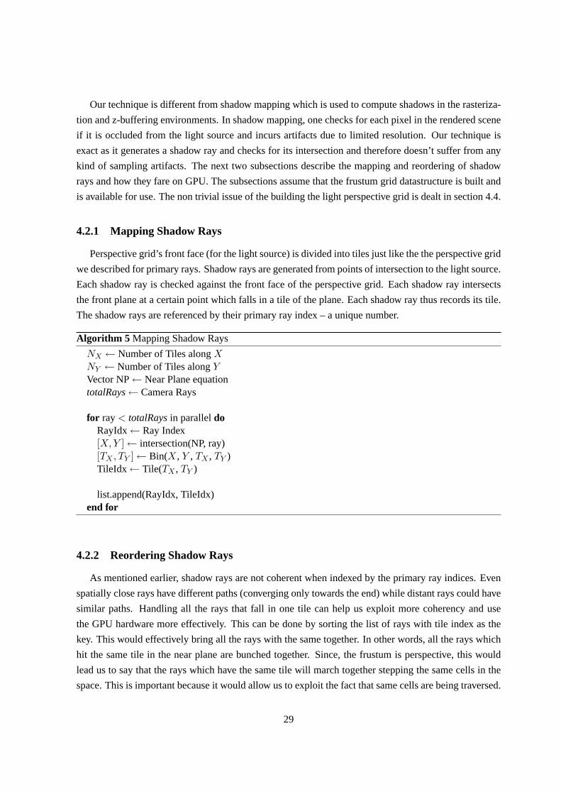
Our technique is different from shadow mapping which is used to compute shadows in the rasteriza-
tion and z-buffering environments. In shadow mapping, one checks foreach pixel in the rendered scene
if it is occluded from the light source and incurs artifacts due to limited resolution. Our technique is
exact as it generates a shadow ray and checks for its intersection and therefore doesn’t suffer from any
kind of sampling artifacts. The next two subsections describe the mapping and reordering of shadow
rays and how they fare on GPU. The subsections assume that the frustumgrid datastructure is built and
is available for use. The non trivial issue of the building the light perspective grid is dealt in section 4.4.
4.2.1 Mapping Shadow Rays
Perspective grid’s front face (for the light source) is divided into tilesjust like the the perspective grid
we described for primary rays. Shadow rays are generated from points of intersection to the light source.
Each shadow ray is checked against the front face of the perspective grid. Each shadow ray intersects
the front plane at a certain point which falls in a tile of the plane. Each shadow ray thus records its tile.
The shadow rays are referenced by their primary ray index – a unique number.
Algorithm 5 Mapping Shadow Rays
NX ← Number of Tiles alongXNY ← Number of Tiles alongYVector NP← Near Plane equationtotalRays← Camera Rays
for ray< totalRaysin paralleldoRayIdx← Ray Index[X, Y ]← intersection(NP, ray)[TX , TY ]← Bin(X, Y , TX , TY )TileIdx← Tile(TX , TY )
list.append(RayIdx, TileIdx)end for
4.2.2 Reordering Shadow Rays
As mentioned earlier, shadow rays are not coherent when indexed by the primary ray indices. Even
spatially close rays have different paths (converging only towards the end) while distant rays could have
similar paths. Handling all the rays that fall in one tile can help us exploit more coherency and use
the GPU hardware more effectively. This can be done by sorting the list ofrays with tile index as the
key. This would effectively bring all the rays with the same together. In other words, all the rays which
hit the same tile in the near plane are bunched together. Since, the frustum is perspective, this would
lead us to say that the rays which have the same tile will march together stepping the same cells in the
space. This is important because it would allow us to exploit the fact that samecells are being traversed.
29

Triangles of a cell loaded in fast shared memory are used and reused byall the rays in that cell. Similar
to primary rays, loading of triangle data is ammortized and spatial coherency isutilized.
However, to gain the benefits of coherent rays, one has to be able to reorder the rays efficiently
on GPU. Inefficiently reordering rays might lead to decrease in speedups. Also, if the time needed
to reorder the rays and the time needed to traverse these roordered raysis roughly equal to traversing
incoherent rays, the method might not be useful. However, reorderingcan indeed be performed using
simple operations, which can be processed in parallel, taking advantage ofthe GPU architecure to secure
speedup. Reordering is nothing but sorting a key-value pair array on the basis of keys. Here, Tile Index
is the key while Ray Index is the value. At the end of sorting, we have the rays shuffled among each
other but all the rays having same Tile Index are bunched together. Thuswe have all coherent rays
together. A simple check function (kernel in GPU terminology) can determine where the boundaries of
each Tile Index lie and demaracate where rays of one tile end and another begin.
Unlike sorting of triangles, this is sorting of rays. The number of rays to be sorted is bound by the
number of pixels in the image and therefore the number of key-value pairs to be sorted always remains
same. This might change in case of true secondary diffuse rays (like the ones used in pathtracing) as the
rays in each step might vary and thus the number of the key-value pairs to besorted. Our images are
1024 x 1024 pixels large and therefore have1048576 (1M) key-value pairs to be sorted. 1M key-value
key pairs can be sorted in about3.5 ms on GPU. This time is more or less constant for all scenes. The
small overhead of sorting leads to significantly faster results using coherent rays. Sorting is done using
radix sort [43]. As architectures evolve and faster sorting algorithms arrive, speeds will increase even
more [30].
4.3 Load Balancing Shadow Rays
Primary rays had a fixed number of rays going through each tile equal to thenumber of pixels in it.
This decides the number of CUDA threads and blocks to be used. A little experimentation can allow
us to gauge the optimum number of threads and blocks to call. However the number of shadow rays in
each tile is not the same. Areas with large number of primary rays intersectionsspawn a large number
of primary rays which in turn populate the tiles they pass through. In that case, a few tilest might be
populated very heavily while others remain largely vacant. Such a situation is highly unfavourable on
GPU as this would lead to improper load on GPU multiprocessors.
4.3.1 Hard and Soft Boundaries
A load balancingscheme gives us an opportunity to distribute the load such that all CUDA blocks
assigned would have an equitable load. A threshold numberNt of rays is decided and the number of
rays in each block should be kept to a maximum of that number. A perfect load balanced scheme, i.e.,
each block having a threshold number of rays is not possible. There will be tiles where the number
30

of rays is fewer than the threshold. Other rays cannot be accomodated with these rays as they traverse
some other tile.
��������
��������
����������
����������
��������
��������
��������
��������
��������
��������
����������
����������
��������
��������
��������
��������
��������
��������
��������
��������
������
������
����������
����������
��������
��������
��������
��������
��������
��������
������
������
����������
����������
��������
��������
��������
��������
��������
��������
������������
������������
������������
���������������
���������������
���������������
���������������
���������������
���������������
������������
������������
������������
���������������
���������������
���������������
���������������
���������������
���������������boundaries
get
chunksinto
break compactlistsorting
Figure 4.2 Reordering illustrated. Different colors correspond to different cells. Sorting results in allthe same colors coming together.Get Boundariesgets the locations where enumeration of a new cellstarts. Based on a therhold value (in this figure3), rays are divided into chunks and compacted in a tightarray.
In the sorted array, indices are demarcated where rays of one block end and where the rays of other
block begin. We call this demarcation as thehard boundary. Rays across hard boundaries can not be
accomodated together in one CUDA block. For example, if there arek rays in one tileTk andm rays in
tile Tm wherek+m < Nt, these rayscannotbe merged as they deal with two different tiles. If merged,
threads would have to load triangles from two different cells and the rays would check triangles from
both the cells thus significantly increasing the load on the CUDA block unnecessarily. On the other
hand if k > Nt rays are in a tile, they are broken down into chunksNt rays and each distributed on
a different CUDA block. We call such a chuck demarcation as thesoft boundary. Soft boundaries lie
between two hard boundaries and indicate the number of blocks which the rays can be divided into. A
large number of soft boundaries between two hard boundaries indicate alarge number of rays in a single
tile, denoting a large population in a small area.
Suppose a light tile hasR > r rays mapping to it, wherer is the number that a thread block can
handle efficiently. We assign⌈R/r⌉ blocks in the CUDA program to this tile. Other tiles are mapped
to one thread block each, after eliminating empty ones. The total number of thread blocks needed is
Ctotal =N∑
j=1
⌈Rj/r⌉, whereRj is the number of rays in tilej.
On GPU, we use CUDPP [45] primitives to determine hard and soft boundaries and thus demarcate
the rays falling in different tiles. Figure 4.2 shows the pipeline we follow. Therays which were de-
termined used a mapping technique are ordered by their ray ID. Sorting primitive sorts them based on
their tile ID. In the figure, rays having same tile ID have same colors. As a result of sorting, all the
rays with same color come together. A subsequent step to mark the boundaries will get us the boundary
indices. A segmented scan on it gives the number of values having the same key (color). This allows us
31

Algorithm 6 Reordering Load Balancing Shadow Rays
totalrays← image size
for ray<totalraysin paralleldoMappingFunc(tileIDArr[ray], rayIDArr[ray])pseudoArr[ray]← 0scratchArr[ray]← 1oArr[ray]← 0
end for
sort(tileIDArr, rayIDArr)getBoundaries(tileIDArr, pseudoArr)segScan(pseudoArr, scratchArr)getChunks(scratchArr, validArr)numBlocks← compact(validArr, oArr)
to break this (possibly huge) packet of rays into multiple sizeable chunks. This is done by marking the
boundaries on the existing array which had the hard boundaries. Everyhard boundary (different key) is
also a soft boundary (mapped to a different CUDA block.) To keep trackof the first ray in each block,
we do a stream compaction (compaction primitive in CUDPP) step and shrink the number of cells (in
the spherical grid space) toCtotal. In Figure 4.2,r = 3 is used. Thus we have a list of locations to the
values each of which belong to a different CUDA block. The differencebetween two adjacent terms in
the array gives us the number of rays belonging to that CUDA block. This completes our load balancing
step and we invoke as many CUDA blocks as the number of elements in the compacted array.
4.4 Spherical Grid Mapping
In the discussion, we have treated light as a camera which has a point of origin and shoots rays in
a direction. Since our light source is a point light, it has a point of origin butshoots light rays in all
direction and not a particular direction. If we create a perspective grid ina single direction, we would
have shadows only in that direction. For models that can be bounded in a frustum, this is great as it
would lead to generate correct shadows.
However, in an architectural scene or a scene with objects all around and light inside the scene or
the model world, a frustum can not be created. Figure 4.3 shows the difference in the twocases. In
the second case, only a subset of triangles is bounded and the resultantshadows would be incorrect.
Therefore, one has to bound all the triangles and make sure all the triangles in the path between the
primary intersections and light source participate in shadow checking.
Since, light rays emanate in all possible directions and since we need to cover all the light rays, we
use a way to divide the world into zones (or tiles.) This can be done by any unbiased mapping system
32

Figure 4.3 Light outside the scene bounding all the triangles and light among the trianglesand notbounding the model.
which can map any point in the world uniquely into other system. We use a small variant of spherical
mapping system to identify each unique point in the world and map it to a tile in the grid.
θ
αO O θ
α−π
−π/2
π/2π
Figure 4.4Spherical space used for shadows.
A light frustum is constructed in theα-θ space whereα andθ are respectively the azimuthal and
elevation angles (longitude-latitude scheme). Figure 4.4 shows the spherical space with respect to the
forward, right and up directions. A rectangle in theα-θ space defines the light frustum and plays the
role of the image for primary rays. We define “tiles” on this rectangle to build cells of the grid using
constant depth planes. The angleα is measured from the forward direction in the forward-right plane
and the angleθ is measured from the up direction in the forward-up plane. Lower and upper limits on
the distance from the light source play the role of near and far planes. This method however suffers
from the demerit of pole singularity. All triangles lying in the right-forward plane (θ is π2), will be
duplicated along all the tiles near the pole. This loss in performance can be mitigated by choosing a
”good” forward direction. Choosing the line joining the light position to the centroid of the model helps
us limit the number of triangles along the pole.
33

Figure 4.5Triangles included for shadow checking.
Spherical mapping of this kind treats all directions equally, in an unbiased fashion. We would ideally
want to handle only that geometry which is visible and also only include the geometry that lies in the
line of sight from these triangles to the light position. We can do this by bounding the light frustum
to the include only the bounding box of the camera’s frustum. Bounding the camera’s frustum would
eliminate many triangles, we can go a step further and eliminate all those triangles also which don’t
lie in the light’s frustum. Since, these triangles don’t lie in the frustum of the light,they will never
participate in shadow checking. This leads to elimination of more triangles which ismuch better from
the point of view of shadow checking as we have lesser triangles to check.
We do this by limiting the angular extents of the light’s frustum to the bounding box of projection
of the camera’s view frustum. Figure 4.6 demonstrates the reduction of triangles participating in the
grid building and ray triangle checking. Furthermore, it devotes the grid tilesto a smaller area, dividing
the area more finely. Instead of devoting area of tiles to triangles which do not participate in shadow
checking, we devote tiles to areas which participate in triangle checking and divide this area more finely.
This technique also points a way to implement spot lights with light fall off. The spot can be marked
as a bounding rectangle in the spherical space shown in Figure 4.6. A cubemap style of ray mapping to
limit light space rays was used earlier [19]. They handle each frustum separately, resulting in a lot of
extra work for the traversals. Furthermore, clamping a cubemap is very tedious when it has to identify
the grid which a ray has to check. In contrast, spherical mapping provides a more unified framework to
compute shadows.
4.5 Results
We tested our techniques of shadow checking on GTX 280 as well as the newer generation GTX 480
hardware. Since shadow rays are not well distributed, we use data rearrangment, which chiefly consists
of mapping the shadow rays to the spherical map, sorting the rays, binning them and performing stream
compaction. The number of (image space) shadow rays is always constant or atleast known at runtime
34

������������������������������������������������������������������������������������������������������������������������������������������������������������������������������������������������������������������������������������������������������������������������������������
������������������������������������������������������������������������������������������������������������������������������������������������������������������������������������������������������������������������������������������������������������������������������������
������������������������������������������������������
������������������������������������������������������
D
A B
C
(−π,π/2)
(−π,−π/2) (π,−π/2)
(π,π/2)
Figure 4.6Bounding rectangle of the geometry in spherical space defines the light frustum of interest.
and does not change over scenes and models. Therefore reordering operation is nearly constant over all
scenes. The mapping operation is embarrasingly parallel and the underlying vector operations SIMD
friendly. The subsequent sort, scan and compact operations are alsoefficient on GPU (provided the data
is large.) Figure 4.7 shows the times taken by different scenes for the rearragement of their shadow rays.
The resolution of the image was1024 X 1024 resulting in1048576 shadow rays.
Figure 4.7Time taken for rearrangement of shadow rays for shadow checking.
Building the shadow grid acceleration data structure takes more time than buildingan analogous one
for primary rays. This, however depends on the number of triangles in thesorting step. Morever, in
the shadow grid building step, there is an additional overhead of spherical grid mapping which leads
to higher times. This involves getting the bounds of the camera frustum and thenrestricting it to the
bounds of the light frustum. This is done over two kernels which need to be invocated from the host
and therefore consume time. Figure 4.8(a) shows the times taken to build shadow datastructure which
35

includes time the light space grid and clamping. Happy Buddha model has distinctly higher cost due to
its higher triangle count. Otherwise one can notice that the overhead of computing the spherical map is
not too high.
Figure 4.8(a) Time taken for building perspective grid from point of view of light. Timings also includetime taken to compute spherical grid mapping and rearrangement of shadow rays for shadow checking.The plot also shows the times taken to construct a uniform grid for the same scene. (b) Time taken byshadow rays to traverse the datastructure. UG is Uniform Grid [23], PG isour method and SBVH isSpatial BVHs [47].
Fairy Sibenik Conference HappyOur [23] Our [23] Our [23] Our [23]
Primary DS Build 3.92 16.65 3.11 9.22 4.11 13.47 9.04 12.04Primary Ray Traversal 5.88 72.26 3.18 54.27 2.98 44.25 6.70 40.10
Shadow DS Build 4.19 0.0 3.58 0.0 5.15 0.0 9.08 0.0Data Rearrangement 3.78 0.0 3.69 0.0 3.72 0.0 3.69 0.0
Shadow Ray Traversal 6.09 122.73 5.69 43.73 4.52 46.64 8.43 81.18Total 23.86 211.68 19.25 107.22 20.48 104.36 36.94 133.32FPS 41.9 4.72 51.94 9.32 48.83 9.58 27.07 7.50
Table 4.1Time in milliseconds for primary and shadow rays for different stages for our method andan implementation of Kalojanov et al. [23]. They use a uniform grid structurefor primary and shadowrays. Times are on a GTX480 GPU.
The traversal of the light frustum is often dependent on the distance of the light source from the
scene. As light moves away from the scene, more rays get bundled in the same tiles and there is a large
disparity in the populations of the cells. However load balancing alleviates this problem. Rays falling
in the same tile are broken into chunks for separate processing in different CUDA blocks. Figure 4.9
shows the variation of the time taken to compute shadows as a function of distance from (center of)
the model. Light moves away in the direction of the line joining the light to the center of the model.
While other bins show a steady rise,64 rays per bin provides a consistent performance and mitigates
36

3 4 5 6 7
20
40
60
distance from light (in model units)
Tim
e(i
nm
s)
64 Rays 128 Rays 256 Rays
Figure 4.9 Time taken as a function of distance of light from Fairy model. Times were takenfor thechunks of three different bin size – 64, 128 and 256. Timings were as noted on GTX 280.
the problem of changing light to a great extent. Having256 rays in a single bin meant more threads
having to cooperate and march together. Also, since256 is a large number, it would mean few overall
CUDA blocks and is almost equivalent to a situation without load balancing. Onthe other hand,64 rays
per chunk lead to larger number of blocks with moderate sized block sizes. The loads are more or less
equally divided and this size remains robust as light moves away from the model.
Overall, the traversal times for shadow rays in perspective grid based method are quite low and are
almost in line with SBVH based traversal in some cases. Traversal of uniform grid is quite slow and will
lead to poor frame rates. Figure 4.8(b) gives the comparison of the times among these three methods.
The table’s analysis is incomplete and inaccurate without taking into account the fact that to make the
traversal as competitive as BVH, we need to build the grid everyframe or everytime the scene changes.
In case of BVH and uniform grid, one needs to rebuild the datastructure only when the scene geometry
changes. In the case of perspective grid datastructure, one needs torebuild it even if light position
changes.
As discussed already, a scene is either a static scene or a dynamic scene.View independent datastruc-
tures like BVHs, kdtrees and uniform grids need to build datastructures only when the scene is dynamic.
View dependent methods like perspective grids need to be rebuilt when theposition of viewing changes.
In case of light, also when the position of the light changes. For dynamic scenes, the time taken by
various datastructures to trace primary and shadow rays is given by
tbvhtotal = {{tbvh
ds + tptrace + tshtrace} × L} × N
tugtotal = {{tug
ds + tptrace + tshtrace} × L} × N
37

tpgtotal = {{tug
ds + tpds + tptrace + {tshds + treorder + tshtrace} × L} × N
Right now, there are no parallel implementations of SBVH. Sequential build onCPU take72 seconds
to build the hierarchy for a model like Happy Buddha with1.09M triangles. In constrast, uniform grid
takes 12 ms on GPU. Perspective grid takes7 ms. For number of lights, L, if we plug in the values
from table 4.1 and plot 4.8, we arrive at a condition between the number of lights and the time taken to
build the SBVH asL =tbvh
ds− 9
14. A plot of the relationship is shown in plot 4.10. We started with160
ms because the GPU implementation of SBVH will be atleast as high as HBVH [36] which is currently
builds in that time.
Figure 4.10Plot showing the number of lights required in a scene to let a per-frame built SBVH to befaster than a per-frame per-pass built grid. Numbers are for Happy Buddha Model.
We can see that for scenes with small number of lights, grid is better becauseof cheap construction of
perspective grid and its packetized traversal. However, as the lights increase, the number of frustums to
be built increases and that is where SBVH starts outperfroming. The one timecostly rebuild of SBVH
handles lights from all directions in about the same way and shows less dropin performance as the
number of lights scale. An SBVH implementation with a build time of400 ms and more than 28 lights,
using a per-frame rebuilt SBVH is cheaper than using a grid which builds a perspective grid from the
point of view of each and every light source and traces the rays.
38

Chapter 5
Coherence in Reflection Rays
Hell, there are no rules here,
we are trying to accomplish something.
– Thomas A. Edison
Reflection rays, in many ways are representative of the general secondary ray. They may not possess
a sense of direction, spreading out in all directions. Unlike primary rays and shadow rays, there is
no preferred direction and therefore perspective grids may not be useful for reflection rays. In case of
multiple lights, one had very few directions to take care of and rebuilding the datastructure was less
expensive than inefficient traversal of a uniform grid datastructure.In the case of reflection rays, the
number of directions in the worst case can be as high as the number of raysthemselves. Therefore it is
better to build a datastructure once and use it for traversals. The acceleration datastructure needs to be
built in each frame as the scene is dynamic, but there no preferred directions for coherence.
Since uniform grid is inexpensive to build compared to BVH, we build a uniform grid. We build
the grid similar to the one proposed in Kalojanov and Slusallek [23] on GPU. The method of building a
uniform grid is similar to the construction of perspective grid. We skip the VFCand BFC test and check
the triangles against the bounding box of the cells in the scene. These uniformly sized cells are formed
by dividing the bounding box of the scene into equal volumed regions. Triangles are checked against
these volumes and cell-triangle pairs are created (similar to the perspective grid method.) A subsequent
sort, scan and stream compaction would give the list of triangles in each cell.
Since the rays do not have any fixed direction, triangles can not be eliminated by using Back Face
Culling (BFC). Also, since the grid is not a frustum and covers the entire volume of the scene, triangles
can not be eliminated using View Frustum Culling (VFC) either. Kalojanov and Slusallek [23] traverse
the resultant grid using a method called outlined by Amanatides and Woo [4]. This algorithm involves
each ray independently walking from one cell to another. We call this methodIndependent Voxel Walk
algorithm. We also explore a method to form a list of the cells a ray is traversing and enforce some
coherence by processing all rays through each cell simultaneously in order to make the reflection more
GPU friendly. We call this procedureEnforced Coherencemethod.
39

5.1 Independent Voxel Walk (IVW)
Each ray can walk along the voxels it encounters by computing the next voxel, starting with its
starting point. Each ray checks intersection by loading the triangles of the voxel it encounters. This
continues until the first intersection is found, when the ray terminates. In a voxel, since there is no
ordering among the triangles, closest intersection is declared after checking against all triangles in it.
Algorithm 7 illustrates the algorithm in form of a pseudocode.
Algorithm 7 Independent Voxel Walk
totalrays← image size
for ray<totalraysin paralleldowhile ray has not found intersectiondo
voxel← determineVoxel(ray)for all triangles in voxel in serialdo
checkIntersection()if found intersectionthen
breakend if
end forend while
end for
Traversal and triangle checking are very tightly knit in this very simple algorithm which does not
assume any coherence. The lack of coherence can incur heavy penalties on older generation GPUs
with large SIMD width and no caching. Large SIMD width would mean that a moderate number of
rays have to check for intersection together. But if these rays are not spatially close or diverging, the
trangles which need be picked may not be the same causing a large number ofglobal accesses and
considerable slowing down of the entire process. Caching exploits locality that may be present across
threads. The newer Fermi architecture has a moderate L1 cache sharedamong a group of processors in
a multiprocessor (MP) and a large L2 cache common to all processors. TheL1 cache can be shared by
the threads of a CUDA block and the L2 cache be used by all the threads. The independent voxel walk
method can benefit from these simple caches if multiple rays are checking intersection for the same
voxel simultaneously or close together in time. Even if the possiblity of being spatially close is remote,
caching can exploit the least bit of coherence by minimizing the number of global memory accesses. L2
cache is fairly large and can hold a large number of triangles’ data and serve as a slightly faster global
memory with lesser penalty. As future GPUs and manycore architectures arelikely to have even more
flexible caching mechanisms, this type of approach will benefit from improvements in architectural
improvements.
40

5.2 Enforced Coherence
Tracing primary rays is totally coherent because we can identify groups of rays which pass through
the same cell at the same time. The triangles of the cell are brought together to the shared memory and
the intersection calculations can be performed from the shared memory. We can enforce coherence by
processing all rays that pass through the cell together.
Enforcing coherence involves reordering the rays to force a conditionof coherence. To do this, we
first determine the cells which each ray passes through to get a list of (ray, cell) pairs. We sort this list on
the cell ID to bring all the rays passing through that cell together. The rays are all shuffled but spatially
close rays come together, We can now use a technique similar to primary raytracing to get the triangle
data to shared memory. We can allocate a CUDA block to each cell but that mightlead to enequitable
distribution of load. Reflection rays like any secondary rays can be concentrated in a small place leading
to disproportionate balance of load. Therefore a load balancing step is necessary to divide the load into
chunks and process them using different CUDA blocks.
While this method is good at enforcing coherence, it comes at the cost of losing the ordering of
the ray’s traversal. A ray traverses the grid in certain order and this ordering helps us determine the
closest intersection without having to proceed through all the cells. However, with sorting the ordering
is lost and the cells are shuffled. Since different rays have differing directions, there can’t be a strategy
to quickly decide the order on basis of cell IDs either. The correct way itis to process all the cells
and everytime one gets an intersection, check if it is the minimum for that ray anddo so till the end
of the traversal. If a ray passes through multiple cells, it will checked by multiple CUDA blocks,
possibly concurrently. Therefore when the rays update the closest intersection, updating should be done
atomically. Since this updating is done on a global level, it becomes an overhead. In our method, we
perform atomic operations first on shared memory and then one update perCUDA block into the global
memory. This reduces the number of the global memory writes considerably. The pseudocode of the
Enforced Coherence method is outlined in Algorithm 8
The first step in intersection checking is to bring the triangle data in the sharedmemeory. This is done
by the threads in the CUDA block, each of which which bring data of one triangle from global memory.
For cells which have more triangles than the number of threads, triangles arebrought in batches. Each
batch is completely used before loading the next batch of triangles. As already mentioned, the ordering
is lost, due to which rays can not be terminated on basis of finding an intersection. One has to find all
intersections and then get the closest among them.
Due to the large number of elements to be dealt with, reordering is computationallyintensive and
memory intensive. The number of (ray ID, cell ID) pairs for a typical conference room scene is about10
million pairs, as each ray passes through10 cells on an average. This number only indirectly depends
on the geometry of the scene through reflection ray origins and directions.The sorting operations are
fast on today’s GPUs and have been getting better over the years. The overhead incurred in reordering
and minimum finding can be offset by the coherence we obtain using this method.
41

Algorithm 8 Enforced Coherence Method
totalrays← image size
for ray<totalraysin paralleldocountArr[ray]← 0countArr[ray]← DetermineVoxels(ray)
end for
totalvoxels← 0for ray<totalraysin paralleldo
totalvoxels← totalvoxels+ countArr[ray]end for
allocate memory(tileIDArr, rayIDArr)
for ray<totalraysin paralleldoDumpVoxels(rayIDArr[ray], tileIDArr[ray])
end for
for i<totalvoxelsin paralleldopseudoArr[i]← 0scratchArr[i]← 1oArr[i]← 0
end for
sort(tileIDArr, rayIDArr)getBoundaries(tileIDArr, pseudoArr)segScan(pseudoArr, scratchArr)getChunks(scratchArr, validArr)numBlocks← compact(validArr, oArr)
for all blocks in numBlocksdowhile all rays in blockdo
load triangles to shared memorycheck for intersection
end whileend for
for rays<totalraysin paralleldoget minimum of all intersections
end for
42

5.3 Results
Due to faster sorting times, the time taken to build the uniform grid is less than the times inthe paper
of Kalojanov and Slusallek [23]. Furthermore, this grid is constructed onlyonce. Since the construction
of perspective and uniform grid is almost the same with slight difference, many of the steps can be
merged. However, we found that the common steps have little overhead while the non common steps
are the ones that can not be merged resulting in little difference in the two methods. We have pursued
the method of computing the uniform grid separately.
The difference in times between the construction of uniform and perspective is due to the larger
number of triangles in uniform grid. Because we do not eliminate triangles using BFC and VFC, we
have the same number of triangles as the number of triangles in the original triangle soup. A part of this
difference is already shown in figure 3.6.
Figure 5.1 The models and viewpoints used for evaluation of the performance of reflection rays. Themodels are Conference Room (284k), Happy Buddha (1.09M) and Fairy Forest (174k). The Buddhamodel has the reflection parts coloured white.
We compare the performance of the IVW and EC methods on different GPUs. For this analysis, we
used a128× 128× 128 voxel resolution for all scenes. The resolution we have used is not impervious
to problems. A long thin object might have problems with such a resolution as dividing the object along
its thin axes would lead to unnecessary overhead. In most of our scenes, except a few scanned models
like Dragon or Happy Buddha, all are equally distributed over the three axes and such a division is
suitable. However, an interesting future work would be alalyze the model and come up with a model
driven resolution to accomodate the triangle data in a judicious manner. On GPU, We used radixsort
from CUDPP [43] to sort the ray-voxel pairs. We focus on three representative models for this analysis.
Conference Model: This model has a room with a table, a few chairs, and walls. This model
has triangles reasonably uniformly distributed in the scene space and has largely horizontal or vertical
triangles. As a result, the reflection rays behave well and may have a high degree of coherence.
Fairy in the Forest Model: This model is mostly sparse with dense geometry at a few locations in
space. The normals vary considerably which makes the reflection rays quite incoherent.
43

Buddha Model: This is a scanned model with all the geometry bunched in a tight space. The model
is finely tessellated because of which the normals vary considerably in nearby areas. Since the number
of triangles are high, intersection checking might dominate the tracing time. For this study, we render
the model by itself, with reflections only from itself.
model GPU DS ray,cell cuda ec ivw speedupbuild pairs blocks reorder trace total trace ivw/ec
conference280 31.16
10.46 M 262 K98.46 158.62 257.03 247.61 0.96
480 13.47 57.21 40.12 97.33 36.92 0.37
fairy280 37.31
15.57 M 191 K152.23 252.51 404.74 679.76 1.67
480 16.65 87.54 37.22 124.76 59.77 0.47
happy280 25.43
2.61 M 190 K28.61 101.18 129.79 263.62 2.03
480 12.04 15.56 43.71 59.27 32.43 0.54
Table 5.1Time in milliseconds for reflection rays in each of the broadly classified stages. The fourthcolumn gives the number of ray-voxel pairs created during the enumeration of rays and the fifth col-umn gives the number of blocks assigned after compaction step. The last column gives the relativeperformance of the EC and IVW methods.
Table 5.1 summarizes the results on the three models from the viewpoints given in Figure 5.1. The
enforced coherence (EC) method is slower than the independent voxelwalk (IVW) method on the
GTX480, as the latter can exploit the caches well. In contrast, the EC method ismuch faster on the
GTX280 on Fairy and Happy Buddha models. They perform similarly on the Conference model, per-
haps due to the moderate coherence of the reflection rays on this model. Thereordering time of the
EC method is avoided by the IVW method. Table 5.1 also shows the number of ray-voxel pairs created
during the enumeration step. The number is large on models with a lot of empty space and affects the
performance of the EC method, as it needs more data movement for sorting.
0 100 200 300 400 500
0
20
40
60
80
100
Iteration
Per
centa
ge
ofR
ays
Done
Conference Fairy Happy
Figure 5.2Percentage of rays declaring intersection at each step of iteration. Fairygrows very slowly,taking 454 iterations to check reflections. In contrast, conference takes306 iterations. Happy Buddhatakes just 294 iterations before declaring the status of the reflected rays.
44

We analyze the performance of reflection rays on these models. Figure 5.2shows the percentage of
rays that find their intersections as IVW iteration proceeds. An iteration fora ray is the processing of
a single voxel, beginning with the starting voxel. The Buddha model starts slowbut behaves the best
overall with 80% of the rays terminating in fewer than 80 iterations. This is because all reflections are
self reflections which need only a few iterations. Other rays terminate when they cross the bounding box
of the model. The Conference model starts well, but the progress is slowerafter 60 iterations. The Fairy
model starts and progresses slowly, needing over 450 iterations for completion. The timing performance
(Table 5.1) mirrors this directly with Buddha model attaining the best reflection performance.
We study how the reflection rays are distributed among the voxels. The top left of Figure 5.3 shows
the ray concentration by voxels for the first iteration (or set of voxels explored) of the IVW method for
the 3 models. Most voxels of the Buddha model have fewer than 50 rays passing through them, while
the other models have a few hundred voxels with over 400 rays in them. Raysare processed in parallel
by different CUDA threads. If there are more rays in the voxel, the corresponding threads check the
same set of triangles for intersection and reuse the same data. This is a situation that can make good use
of the L2 cache shared by all threads of the GPU (as the threads processing these rays may come from
different streaming multiprocessors). Buddha performs the worst in exploiting the L2 cache, but its
overall performance is best due to early termination seen before. Top right of Figure 5.3 zooms into the
tail of the ray distribution plot. The Conference model outscores the Fairy model with a larger number
of dense voxels. The relatively bad performance on Fairy can be explained partly by this.
The bottom left of Figure 5.3 shows the divergence present within each primary tile or packet of rays
processing the reflection rays. During IVW, the reflection rays are still processed as packets correspond-
ing to the tiles of the primary rays. If the number of voxels in a packet or a tile is low, the IVW method
will have more rays of the CUDA block accessing the same triangles. This will efficiently use the L1
cache. Most tiles have low divergence in both Conference and Fairy models. not on the Buddha model.
The early part of the plot (bottom right of Figure 5.3) shows that the Conference model exhibits lower
divergence than the Fairy model and performs better, as is confirmed by the tracing times we obtained.
Ray distribution and tile divergence are thus good predictors of reflectionperformance. If the triangle
normals are mostly parallel (as with the Conference model), the reflection rays will be largely coherent,
if a coherent packet of rays hits it. This will reduce the tile divergence and improves the performance
with the use of L1 cache. If the triangle distribution is sparse and the triangleshave widely varying
normals (as with the Fairy model), the reflection rays emanate at few places and travel in all directions.
This reduces the number of rays per voxel and diminishes the overall performance.
Figure 5.6 and 5.7 show results for some other scenes like Fairy, Sibenik and Conference with a
simulation in midair. Figure 5.7 places the Dragon-Bunny collision in the Conference Room model.
These frames take 115 ms to 200 ms per frame to render, depending on the distribution of the fractured
dragon triangles.
Figure 5.4 presents a comparison of the tracing times of our method and an SBVH based method on
a GTX480 for reflection rays. Grids offer no advantages to largely incoherent reflection rays whereas
45

0 200 400 600 800100
101
102
103
104
# of rays in a voxel
#ofvoxel
s
Conference
Fairy
Happy
400 500 600 7000
10
20
30
40
50
# of rays in a voxel
#ofvoxel
s
Conference
Fairy
0 10 20 30 40 50 60100
101
102
103
104
# of voxels in a tile
#ofti
les
Conference
Fairy
Happy
0 2 4 6 8 10 12 140
2,000
4,000
6,000
# voxels in a tile
#ofti
les
Conference
Fairy
Figure 5.3Study of triangle and voxel distributions affecting reflection performance.Top left plot showsthe concentration of rays in each voxel. Top right examines the tail of the plot. Longer tail with largernumber of voxels is better for performance. Bottom left shows voxel divergence in each tile. Bottomright examines the front. Higher number of tiles with less divergence is goodfor performance.
SBVH treats reflection rays in a nearly same fashion as other rays. Thus,reflection rays are much slower
in our method, but if we take into account the time needed for SBVH construction, we gain significantly.
However, if rendering a scene requires several reflection or refraction passes, a BVH-based method can
catch up with ours even if the acceleration structure is built every frame. Referring to figure 5.4, we can
see that SBVH gains 25 ms per reflection pass over our method for Happy Buddha model. If SBVH
build time on GPU is 40 times faster than that of CPU, it will take about 80 passes for SBVH to catch
up. Similarly, it will take 35 passes if the implementation is 100 times faster.
For a static scene, the total time taken for primary, shadow and reflection raytraversal is given by
tbvhtotal = tbvh
ds + {tptrace + tshtrace × L + trtrace} × N
tugtotal = tug
ds + {tptrace + tshtrace × L + trtrace} × N
tpgtotal = tug
ds + {tpds + tptrace + {tshds + treorder + tshtrace} × L + tugtrace} × N
46

Figure 5.4Comparison of traversal times between our method (Grid) and SBVH traversal (SBVH) [2]for various passes in a frame, viz. Primary, Shadow and Reflection rays. For shadow and secondary,time taken to rebuild the data structure and rearranging the data is also included.Numbers are as notedon NVIDIA GTX 480.
However, our consideration is scenes which are dynamic, for which the timetaken for building
datastructure is also brought inside the bracket as it is built every frame.
tbvhtotal = {tbvh
ds + tptrace + tshtrace × L + trtrace} × N
tugtotal = {tug
ds + tptrace + tshtrace × L + trtrace} × N
tpgtotal = {tug
ds + tpds + tptrace + {tshds + treorder + tshtrace} × L + tugtrace} × N
Similar to our analysis in for shadow rays, if we plug in values for all the terms and keep the number
of lights to a standard3 and in the best case assume the GPU implementation of SBVH is at low
as as HBVH implmenetation [36] at160 ms, we see that it would take about4 bounces before the
performance of perspective grid based implmentation starts to deteriorate. Plugging in the values and
after a little algebra, we arrive at the condition between number of bouncesand the time required for
building SBVH asB =tbvh
ds− 63
24. A plot of the following condition is figure 5.5. We can see that for
scenes with small number of lights, grid is better because of cheap construction of perspective grid and
its packetized traversal. However, as the bounces increase, the time takenby grid in inefficient traversal
of a uniform grid datastructure increases that is where SBVH starts outperfroming. The one time costly
rebuild of SBVH handles reflections rays from all directions in about the same way and shows less drop
in performance as the number of lights scale. An SBVH implementation with a build time of 500 ms
and more than 18 bounces, using a per-frame rebuilt SBVH is cheaper than using a grid which builds
a perspective grid from the point of view of each and every light source and traces the rays. Similar
calculations for number of passes can help us determine the point where theSBVH starts outperforming
the grid datastructure.
47

Figure 5.5Plot showing the number of bounces required in a scene to let a per-framebuilt SBVH to befaster than a per-frame per-pass built grid. Numbers are for Happy Buddha Model.
48

Figure 5.6 In Fairy and Sibenik, only the floor is reflective. In case of Bunny floating in ConferenceRoom, the wooden table and the wooden frame of the red chairs is a highly polished reflective surface.
49
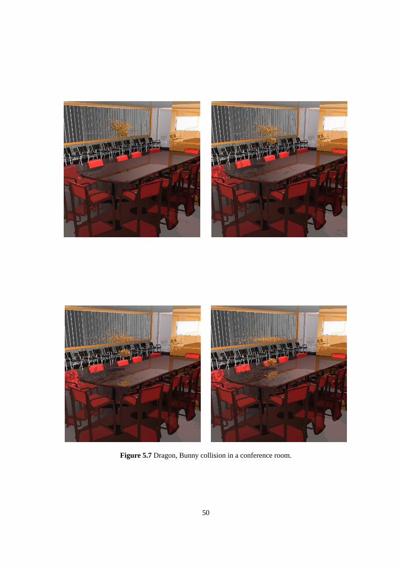
Figure 5.7Dragon, Bunny collision in a conference room.
50

Chapter 6
Discussion and Conclusions
Sentence first,
verdict afterwards.
– Queen of Hearts, Alice in the Wonderland
Most work in speeding up raytracing has looked at various parts of raytracing in an isolated fashion.
There is work on building good quality datastructures but which are costly tobuild. The moderate
or inferior quality datastructures are efficient to build and well parallelizable but are not efficient in
terms of tracing rays. On the other hand, tracing of rays has been handled separately. Performance
benchmarks are presented for rays traversing the best quality datastructure. In the realtime raytracing
context, methods have to be conceived which strike an optimum balance between the goals of building a
good quality datastructure and achieving realtime traversal performance.Through this dissertation, we
have presented various strategies through which we can use grid datastructure to achieve interactive to
near realtime performance consistently. All the methods we propose map and perform very well on the
GPU architecture like Nvidia CUDA and OpenCL.
Often, it is known whether the scene is going to be static or dynamic. Also if it is dynamic, how often
is it going to change. These clues can help us decide a better datastructurefor the purposes of raytracing.
No one datastructure is superior and often it is best to use a datastructurebased on the constraints and
demands. Static scenes are always rendered faster with BVH or Kd-tree. Grid datastructure with its
slow traversal, in the worst case, might result in orders of magnitude slower traversal. However, with
scenes which change dynamically, a datastructure has to be built everytime the scene changes. Here,
the difference in BVH and grid start narrowing down. However, if the number of lights is large, or the
number of passes is high or the scene is being rendered with lots of rays (typical in global illumination),
investing time in a better datastructure might be the right way even for dynamic scenes. Grids are an
attractive choice for game like scenes with changing geometry, few lights andsmall number of passes.
In practical scenarios, there is often high similarity between two frames inspiteof changing geom-
etry. Between any two frames, the number of primitives that might have moved may be tracked with
moderate ease. Also, the existing ordering among the triangles can be used and the triangles flagged as
51

moved can be reinserted into the ordered list. However, updating the datastructure does not map well
to architectures like GPU with fine grained parallelism. These architectures tend to favour large scale
regular operations rather than small scale irregular operations. Adding asmall set of triangles to a large
set of already sorted list of triangles is an example of such a scenario. Sorting an entire array rather than
inserting a few elements is faster on GPU and therefore rebuilding the grid datastructure is ideal in a
GPU setting.
In our experiments, we found that grids perform really well when the number of cells to be traversed
is less. Our approach makes such a scenario possible as we remove triangles using Back Face Culling
(BFC) and View Frustum Culling (VFC). Also, in the case of secondary rays where we use a uniform
grid and resort to single ray traversal using the Independent Voxel Walk algorithm, our technique is able
to take advantage of the fact that rays remain partially coherent for the first few iterations and some
hidden coherency can be exploited if a cache based architecture is present.
Traditionally, building of an acceleration datastructure has been viewed asa necessary overhead.
Most approaches rely on carefully building an acceleration datastructure so as allow smooth and efficient
traversal. Our work is a significant deprature from this CPU based raytracing philosophy as we build the
datastructure multiple times to suit the rays to be traced. We show that the cost ofbuilding a cheap ray
specialized datastructure again and again more than compensates the build time interms of traversal.
This leads to better speeds and tracing larger number of rays before performance starts deteriorating in
the secondary rays stage. Our superior performance in case of secondary rays is due to the this fact,
that we build another frustum from light point of view and handle the shadow in almost same way as
primary rays.
Our main message is to look at different stages of raytracing independentlyand to consider employ-
ing different and more suitable acceleration datastructures for each pass, keeping the total raytracing
time at interactive to near realtime rates.
52

Related Publications
Ray Tracing Dynamic Scenes with Shadows on GPU
Sashidhar Guntury and P. J. Narayanan
Proceedings Eurographics Symposium on Parallel Graphics and Visualization, 2010
Norrkoping, Sweden
Ray Tracing Dynamic Scenes on GPU
Sashidhar Guntury and P. J. Narayanan
IEEE Transactions on Visualization and Computer Graphics
53

Bibliography
[1] T. Aila and T. Karras. Architecture Considerations for Tracing Incoherent Rays. InHigh Performance
Graphics, pages 113–122, 2010.
[2] T. Aila and S. Laine. Understanding the Efficiency of Ray Traversal on GPUs. InHigh Performance
Graphics, pages 145–149, 2009.
[3] P. Ajmera, R. Goradia, S. Chandran, and S. Aluru. Fast, parallel, gpu-based construction of space filling
curves and octrees. InProceedings of the 2008 symposium on Interactive 3D graphics and games, I3D ’08,
pages 10:1–10:1. ACM, 2008.
[4] J. Amanatides and A. Woo. A Fast Traversal Algorithm for Ray Tracing. InEurographics, pages 3–10,
1987.
[5] G. E. Blelloch. Prefix sums and their applications. Technical Report CMU-CS-90-190, School of Computer
Science, Carnegie Mellon University, Nov. 1990.
[6] J. Bloomenthal and K. Ferguson. Polygonization of non-manifold implicit surfaces. InProceedings of the
22nd annual conference on Computer graphics and interactive techniques, SIGGRAPH ’95, pages 309–
316, New York, NY, USA, 1995. ACM.
[7] B. C. Budge, T. Bernardin, J. A. Stuart, S. Sengupta, K. I.Joy, and J. D. Owens. Out-of-core Data Manage-
ment for Path Tracing on Hybrid Resources. volume 28, pages 385–396, 2009.
[8] R. L. Cook, L. C. Carpenter, and E. E. Catmull. The reyes image rendering architecture. InSIGGRAPH,
pages 95–102, 1987.
[9] H. Dammertz and A. Keller. The Edge Volume Heuristic - Robust Triangle Subdivision for Improved BVH
Performance. InIEEE Symposium on Interactive Ray Tracing, pages 155 –158, 2008.
[10] P. Dutre, K. Bala, and P. Bekaert.Advanced Global Illumination. A. K. Peters, Ltd., Natick, MA, USA,
2002.
[11] M. Ernst and G. Greiner. Early Split Clipping for Bounding Volume Hierarchies.IEEE Symposium on
Interactive Ray Tracing, pages 73–78, 2007.
[12] F. Ganovelli, C. M. (editors, T. Larsson, and T. Akenine-mller. A dynamic bounding volume hierarchy for
generalized collision detection. 2005.
[13] K. Garanzha and C. Loop. Fast Ray Sorting and Breadth-First Packet Traversal for GPU Ray Tracing.
Computer Graphics Forum, 29(2):289–298, 2010.
54
[14] J. Goldsmith and J. Salmon. Automatic creation of object hierarchies for ray tracing.IEEE Comput. Graph.
Appl., 7:14–20, May 1987.
[15] H. Gouraud.Computer display of curved surfaces. PhD thesis, 1971. AAI7127878.
[16] M. Gross. Getting to the point...?IEEE Comput. Graph. Appl., 26:96–99, September 2006.
[17] V. Havran. Heuristic ray shooting algorithms. 2000.
[18] Q. Hou, X. Sun, K. Zhou, C. Lauterbach, D. Manocha, and B.Guo. Memory-scalable gpu spatial hierarchy
construction. Technical report, MSR Asia, UNC, Chapel Hill, 2009.
[19] W. Hunt and W. Mark. Ray Specialized Acceleration Structures for Ray Tracing. InIEEE Symposium on
Interactive Ray Tracing, pages 3–10, 2008.
[20] T. Ize, P. Shirley, and S. Parker. Grid Creation Strategies for Efficient Ray Tracing. InIEEE Symposium on
Interactive Ray Tracing, pages 27–32, 2007.
[21] J. T. Kajiya. Ray tracing parametric patches.SIGGRAPH Comput. Graph., 16:245–254, July 1982.
[22] J. Kalojanov, B. Markus, and P. Slusallek. Two-Level Grids for Ray Tracing on GPUs. InProceedings of
Eurographics (to appear), 2011.
[23] J. Kalojanov and P. Slusallek. A Parallel Algorithm forConstruction of Uniform Grids. InHigh Performance
Graphics, pages 23–28, 2009.
[24] A. Lagae and P. Dutre. Compact, fast and robust grids for ray tracing.Computer Graphics Forum,
27(4):1235–1244, 2008.
[25] C. Lauterbach, M. Garland, S. Sengupta, D. Luebke, and D. Manocha. Fast BVH Construction on GPUs.
Computer Graphics Forum, 28(2):375–384, 2009.
[26] C. Lauterbach, Q. Mo, and D. Manocha. gproximity: Hierarchical gpu-based operations for collision and
distance queries.Computer Graphics Forum, 29(2):419–428, 2010.
[27] C. Loop and J. Blinn. Resolution independent curve rendering using programmable graphics hardware. In
ACM SIGGRAPH 2005 Papers, SIGGRAPH ’05, pages 1000–1009, New York, NY, USA, 2005. ACM.
[28] J. D. MacDonald and K. S. Booth. Heuristics for ray tracing using space subdivision.The Visual Computer,
6:153–166, 1990.
[29] D. Manocha and S. Krishnan. Algebraic pruning: a fast technique for curve and surface intersection.
Comput. Aided Geom. Des., 14:823–845, December 1997.
[30] D. G. Merrill and A. S. Grimshaw. Revisiting Sorting forGPGPU Stream Architectures. InParallel archi-
tectures and compilation techniques (PACT), pages 545–546, 2010.
[31] T. Moller and B. Trumbore. Fast, minimum storage ray/triangle intersection. InSIGGRAPH ’05: ACM
SIGGRAPH 2005 Courses, page 7, 2005.
[32] B. Moon, Y. Byun, T.-J. Kim, P. Claudio, H.-S. Kim, Y.-J.Ban, S. W. Nam, and S.-E. Yoon. Cache-oblivious
Ray Reordering.ACM Transactions on Graphics, 29(3):1–10, 2010.
[33] P. A. Navratil, D. S. Fussell, C. Lin, and W. R. Mark. Dynamic Ray Scheduling to Improve Ray Coherence
and Bandwidth Utilization. InIEEE Symposium on Interactive Ray Tracing, pages 95–104, 2007.
55

[34] J. Nickolls, I. Buck, M. Garland, and K. Skadron. Scalable Parallel Programming with CUDA.ACM Queue,
6:40–53, 2008.
[35] Nvidia. Cuda SDK.
[36] J. Pantaleoni and D. Luebke. HLBVH: Hierarchical LBVH Construction for Real-Time Ray Tracing. In
High Performance Graphics, pages 87–95, 2010.
[37] S. Patidar and P. Narayanan. Scalable Split and Gather Primitives on the GPU, IIIT/TR/2009/99. Technical
Report IIIT/TR/2009/99, 2009.
[38] S. Patidar and P. J. Narayanan. Ray Casting Deformable Models on the GPU. InIndian Conference on
Computer Vision, Graphics and Image Processing, pages 481–488, 2008.
[39] M. Pharr, C. Kolb, R. Gershbein, and P. Hanrahan. Rendering Complex Scenes with Memory-Coherent Ray
Tracing. InSIGGRAPH, pages 101–108, 1997.
[40] B. T. Phong. Illumination for computer generated pictures.Commun. ACM, 18:311–317, June 1975.
[41] S. Popov, I. Georgiev, R. Dimov, and P. Slusallek. Object Partitioning Considered Harmful: Space Subdivi-
sion for BVHs. InHigh Performance Graphics, pages 15–22, 2009.
[42] T. J. Purcell, I. Buck, W. R. Mark, and P. Hanrahan. Ray tracing on programmable graphics hardware. In
Proceedings of the 29th annual conference on Computer graphics and interactive techniques, SIGGRAPH
’02, pages 703–712, New York, NY, USA, 2002. ACM.
[43] N. Satish, M. Harris, and M. Garland. Designing Efficient Sorting Algorithms for Manycore GPUs. In
IEEE IPDPS, pages 1–10, 2009.
[44] J. Schmittler, S. Woop, D. Wagner, W. J. Paul, and P. Slusallek. Realtime Ray Tracing of Dynamic Scenes
on an FPGA Chip. InGraphics Hardware, pages 95–106, 2004.
[45] S. Sengupta, M. Harris, Y. Zhang, and J. D. Owens. Scan Primitives for GPU Computing. InGraphics
Hardware, pages 97–106, 2007.
[46] M. Stamminger and G. Drettakis. Interactive sampling and rendering for complex and procedural geometry.
In Proceedings of the 12th Eurographics Workshop on RenderingTechniques, pages 151–162, London, UK,
2001. Springer-Verlag.
[47] M. Stich, H. Friedrich, and A. Dietrich. Spatial Splitsin Bounding Volume Hierarchies. InHigh Perfor-
mance Graphics, pages 7–13, 2009.
[48] D. L. Toth. On ray tracing parametric surfaces. InProceedings of the 12th annual conference on Computer
graphics and interactive techniques, SIGGRAPH ’85, pages 171–179, New York, NY, USA, 1985. ACM.
[49] I. Wald. On fast construction of sah-based bounding volume hierarchies. InProceedings of the 2007 IEEE
Symposium on Interactive Ray Tracing, pages 33–40. IEEE Computer Society, 2007.
[50] I. Wald, T. Ize, A. Kensler, A. Knoll, and S. G. Parker. Ray Tracing Animated Scenes Using Coherent Grid
Traversal.ACM Transactions on Graphics, 25(3):485–493, 2006.
[51] I. Wald, W. R. Mark, J. Gnther, S. Boulos, T. Ize, W. Hunt,S. G. Parker, and P. Shirley. State of the Art in
Ray Tracing Animated Scenes. InComputer Graphics Forum, volume 28, pages 89–116, 2007.
56

[52] B. Walter, A. Arbree, K. Bala, and D. P. Greenberg. Multidimensional lightcuts.ACM Trans. Graph.,
25(3):1081–1088, 2006.
[53] M. Wand, M. Fischer, I. Peter, a. d. H. Meyer, Friedhelm,and W. Strasser. The randomized z-buffer
algorithm: interactive rendering of highly complex scenes. In Proceedings of the 28th annual conference
on Computer graphics and interactive techniques, SIGGRAPH ’01, pages 361–370, New York, NY, USA,
2001. ACM.
[54] T. Whitted. An improved illumination model for shaded display.Commun. ACM, 23(6):343–349, 1980.
[55] K. Zhou, Q. Hou, R. Wang, and B. Guo. Real-time KD-tree Construction on Graphics Hardware.ACM
Transactions on Graphics, 27(5), 2008.
57