Naval Research LaboratoryWashington, DC 20375-5320

NRL/FR/7218--04--10,101

Rayleigh-Sommerfeld Diffractionvs Fresnel-Kirchhoff, FourierPropagation, and Poisson’s Spot

ROBERT L. LUCKE

Radio/IR/Optical Sensors BranchRemote Sensing Division

December 30, 2004

Approved for public release; distribution is unlimited.

i

REPORT DOCUMENTATION PAGE Form ApprovedOMB No. 0704-0188

3. DATES COVERED (From - To)

Standard Form 298 (Rev. 8-98)Prescribed by ANSI Std. Z39.18

Public reporting burden for this collection of information is estimated to average 1 hour per response, including the time for reviewing instructions, searching existing data sources, gathering and maintaining the data needed, and completing and reviewing this collection of information. Send comments regarding this burden estimate or any other aspect of this collection of information, including suggestions for reducing this burden to Department of Defense, Washington Headquarters Services, Directorate for Information Operations and Reports (0704-0188), 1215 Jefferson Davis Highway, Suite 1204, Arlington, VA 22202-4302. Respondents should be aware that notwithstanding any other provision of law, no person shall be subject to any penalty for failing to comply with a collection of information if it does not display a currently valid OMB control number. PLEASE DO NOT RETURN YOUR FORM TO THE ABOVE ADDRESS.

5a. CONTRACT NUMBER

5b. GRANT NUMBER

5c. PROGRAM ELEMENT NUMBER

5d. PROJECT NUMBER

5e. TASK NUMBER

5f. WORK UNIT NUMBER

2. REPORT TYPE1. REPORT DATE (DD-MM-YYYY)

4. TITLE AND SUBTITLE

6. AUTHOR(S)

8. PERFORMING ORGANIZATION REPORT NUMBER

7. PERFORMING ORGANIZATION NAME(S) AND ADDRESS(ES)

10. SPONSOR / MONITOR’S ACRONYM(S)9. SPONSORING / MONITORING AGENCY NAME(S) AND ADDRESS(ES)

11. SPONSOR / MONITOR’S REPORT NUMBER(S)

12. DISTRIBUTION / AVAILABILITY STATEMENT

13. SUPPLEMENTARY NOTES

14. ABSTRACT

15. SUBJECT TERMS

16. SECURITY CLASSIFICATION OF:

a. REPORT

19a. NAME OF RESPONSIBLE PERSON

19b. TELEPHONE NUMBER (include areacode)

b. ABSTRACT c. THIS PAGE

18. NUMBEROF PAGES

17. LIMITATIONOF ABSTRACT

Rayleigh-Sommerfeld Diffraction vs Fresnel-Kirchhoff, Fourier Propagation, and Poisson’s Spot

Robert L. Lucke

Naval Research LaboratoryWashington, DC 20375-5320 NRL/FR/7218--04-10,101

Approved for public release; distribution is unlimited.

Unclassified Unclassified UnclassifiedUL 17

Dr. Robert L. Lucke

(202) 767-2749

DiffractionFourier propagation

National Aeronautics and Space Administration300 E St. S.W.Washington, DC 20024-3210

When the Fresnel-Kirchhoff (FK) diffraction integral is evaluated exactly (instead of using the Fresnel approximation), the well-known mathematical inconsistency in the FK boundary conditions leads to unacceptable results for the intensity of Poisson’s spot. The Rayleigh-Sommerfeld (RS) integral doesn’t have this problem. Fourier propagation is equivalent to RS diffraction and provides another means of deriving a diffraction integral.

JPL

8393

30-12-2004 NRL Formal Report June 2003 to June 2004

Jet Propulsion Laboratory4800 Oak Grove Dr.Pasadena, CA 91109

Poisson’s spot

1251876

CONTENTS

1. INTRODUCTION ................................................................................................................................. 1

2. THE BASIC DIFFRACTION PROBLEM ............................................................................................ 1

3. CALCULATING THE INTENSITY OF POISSON’S SPOT ............................................................... 3

4. DOING DIFFRACTION WITH FOURIER PROPAGATION ............................................................. 4

4.1 Fourier Propagation ..................................................................................................................... 5 4.2 The RS Integral Derived via Fourier Propagation ....................................................................... 6

5. CONCLUSION ...................................................................................................................................... 8

REFERENCES ........................................................................................................................................... 8

APPENDIX A — The Sommerfeld Lemma ............................................................................................... 9

APPENDIX B — Deriving the RS Diffraction Integral via Fourier Propagation ...................................... 11

iii

RS Diffraction vs FK, Fourier Propagation, and Poisson’s Spot 1

____________Manuscript approved September 13, 2004

1

RAYLEIGH-SOMMERFELD DIFFRACTION VS FRESNEL-KIRCHHOFF,FOURIER PROPAGATION, AND POISSON’S SPOT

1. INTRODUCTION

The boundary conditions imposed on the diffraction problem in order to obtain the Fresnel-Kirchhoff (FK) solution are well-known to be mathematically inconsistent and to be violated by the solution when the observation point is close to the diffracting screen [1-3]. These problems are absent in the Rayleigh-Sommerfeld (RS) solution. The difference between RS and FK is in the inclination factor and is usually immaterial because the inclination factor is approximated by unity. But when this approximation is not valid, FK can lead to unacceptable answers. Calculating the on-axis intensity of Poisson’s spot provides a critical test, a test passed by RS and failed by FK. FK fails because (a) convergence of the integral depends on how it is evaluated and (b) when the convergence problem is fixed, the predicted amplitude at points near the obscuring disk is not consistent with the assumed boundary conditions. Poisson’s spot, also known as the spot of Arago, is the name given to the bright on-axis spot behind a circular obscuration illuminated by a plane wave: on the axis of the disk, all light diffracted at the rim of the disk arrives in phase and interferes constructively. Consequently, even for angles approaching 90°, i.e., for observation points close to the disk, diffraction can result in a significant intensity. (In the overwhelming majority of optics problems, diffraction at angles of more than a few degrees leads to vanishingly small intensities and can be safely ignored.) Treatments of Poisson’s spot that make the Fresnel approximation [4,5]

do not apply to the region close to the disk. Treatments that do apply close to the disk use the RS integral [6] or its predecessor, the Rayleigh integral [7]. The RS integral is derived from the Rayleigh integral with the additional assumption that the wavelength of the light is small compared to the geometric dimensions of the problem, an assumption that is made throughout this report. I refer to a calculation as exact to indicate that, while the short-wavelength approximation has been made, the Fresnel approximation has not. The other fundamental approximation made here is the scalar wave approximation, which means that the results apply better to acoustics than to optics, a point that will be reconsidered in the concluding remarks of Section 5. Fourier propagation provides an alternate means of handling diffraction problems. It can be used in computer software to calculate beam propagation problems, but in this report, Fourier propagation theory is used to derive solutions in integral form for the 2-D (long slits and strips) and 3-D (arbitrarily shaped apertures) diffraction problems. Standard Fourier propagation reproduces the RS diffraction integral.

2. THE BASIC DIFFRACTION PROBLEM

Solving the basic diffraction problem requires finding a solution to the Helmholtz equation for a propagating wave encountering a partially obscuring planar screen. The Helmholtz equation is

∇ +( ) =2 2 0k U x y z( , , ) ,

(1)

Robert L. Lucke2

where k = 2π/λ and U describes the amplitude and phase of the wave. U is a scalar, so only scalar diffraction theory is addressed. The boundary condition imposed on the solution to this differential equation is the effect of a diffracting screen in the z = 0 plane. Denoting by T the parts of the screen that are transmissive and by B the parts that block the beam, the boundary conditions used for the RS and FK solutions are

RS and FK: forU x y U x y x y TU x

( , , ) ( , , ) ( , ) ,( ,

0 00= ∈yy x y B

U x y zz

U

z

, ) ( , ) ,( , , )

0 0

0

= ∈∂

∂=

∂

=

for

FK only: 00

0

00

( , , )( , ) ,

( , , )

x y zz

x y T

U x y zz

z

z

∂∈

∂∂

=

=

=

for

forr ( , ) ,x y B∈

(2)

where U0 describes the incident wave and ∂U/∂z is the derivative of U normal to the diffracting plane.

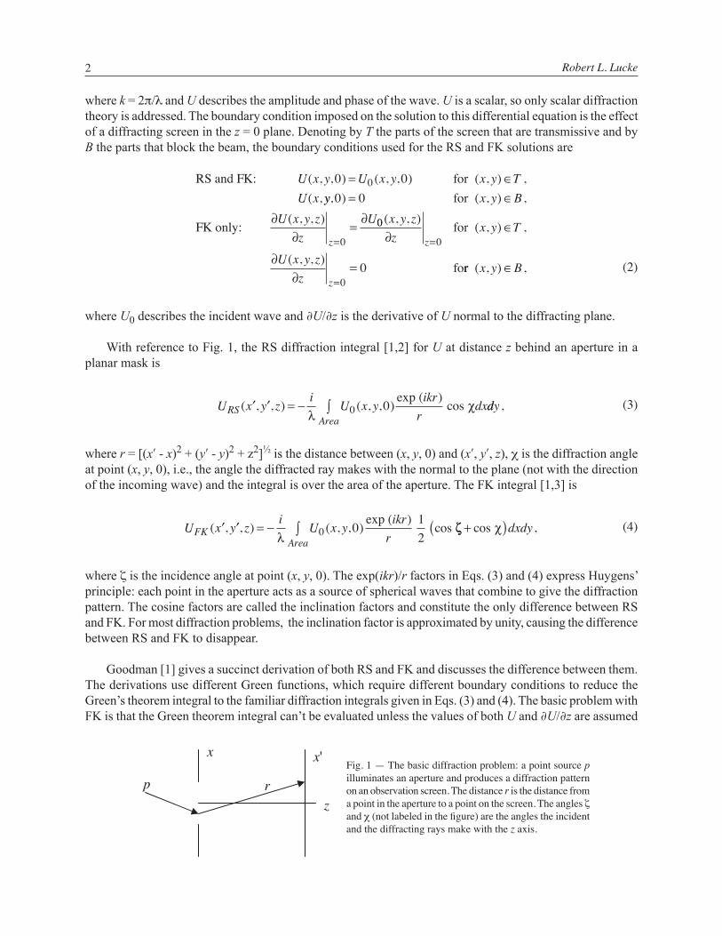
With reference to Fig. 1, the RS diffraction integral [1,2] for U at distance z behind an aperture in a planar mask is

U x y z

iU x y

ikrr

dxRS ( , , ) ( , , )exp ( )

cos′ ′ = −λ

χ0 0 ddyArea

∫ ,

(3)

where r = [(xʹ - x)2 + (yʹ - y)2 + z2]½ is the distance between (x, y, 0) and (xʹ, yʹ, z), χ is the diffraction angle at point (x, y, 0), i.e., the angle the diffracted ray makes with the normal to the plane (not with the direction of the incoming wave) and the integral is over the area of the aperture. The FK integral [1,3] is

U x y z

iU x y

ikrrFK ( , , ) ( , , )

exp ( )cos′ ′ = −

λ 0 012

ζζ χ+( )∫ cos ,dxdyArea

(4)

where ζ is the incidence angle at point (x, y, 0). The exp(ikr)/r factors in Eqs. (3) and (4) express Huygens’ principle: each point in the aperture acts as a source of spherical waves that combine to give the diffraction pattern. The cosine factors are called the inclination factors and constitute the only difference between RS and FK. For most diffraction problems, the inclination factor is approximated by unity, causing the difference between RS and FK to disappear.

Goodman [1] gives a succinct derivation of both RS and FK and discusses the difference between them. The derivations use different Green functions, which require different boundary conditions to reduce the Green’s theorem integral to the familiar diffraction integrals given in Eqs. (3) and (4). The basic problem with FK is that the Green theorem integral can’t be evaluated unless the values of both U and ∂U/∂z are assumed

z

x x'

rpFig. 1 — The basic diffraction problem: a point source p illuminates an aperture and produces a diffraction pattern on an observation screen. The distance r is the distance from a point in the aperture to a point on the screen. The angles ζ and χ (not labeled in the figure) are the angles the incident and the diffracting rays make with the z axis.

RS Diffraction vs FK, Fourier Propagation, and Poisson’s Spot 3

to be zero on the obscuring part of the diffracting screen, but we know from analytic function theory that if both U and ∂U/∂z are zero over any region, then U ≡ 0 everywhere. Thus, the FK solution cannot be fully mathematically consistent and must therefore be suspected of not always (at least) giving the right answer. In Section 3, I use Poisson’s spot to show explicitly that the FK solution can violate the boundary conditions that were assumed for its derivation.

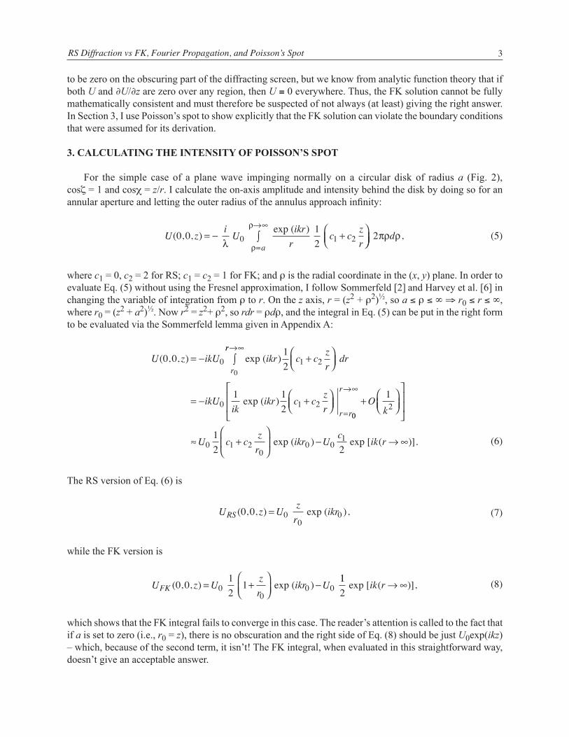
3. CALCULATING THE INTENSITY OF POISSON’S SPOT

For the simple case of a plane wave impinging normally on a circular disk of radius a (Fig. 2), cosζ = 1 and cosχ = z/r. I calculate the on-axis amplitude and intensity behind the disk by doing so for an annular aperture and letting the outer radius of the annulus approach infinity:

U z

iU

ikrr

c czr

( , , )exp ( )

0 0120 1 2= − +

λ =

→∞∫ ,2πρ ρ

ρ

ρd

a (5)

where c1 = 0, c2 = 2 for RS; c1 = c2 = 1 for FK; and ρ is the radial coordinate in the (x, y) plane. In order to evaluate Eq. (5) without using the Fresnel approximation, I follow Sommerfeld [2] and Harvey et al. [6] in changing the variable of integration from ρ to r. On the z axis, r = (z2 + ρ2)½, so a ≤ ρ ≤ ∞ ⇒ r0 ≤ r ≤ ∞, where r0 = (z2 + a2)½. Now r2 = z2+ ρ2, so rdr = ρdρ, and the integral in Eq. (5) can be put in the right form to be evaluated via the Sommerfeld lemma given in Appendix A:

U z ikU ikr c czr

drr

( , , ) exp ( )0 0120 1 2

0

= − +

rr

r rikU

ikikr c c

zr

→∞

=

∫

= − +

0 1 2

1 12

exp ( )00

1

12

2

0 1 20

rO

k

U c czr

→∞+

≈ +

exp ( ) exp [ ( )].ikr U

cik r0 0

12

− → ∞

(6)

The RS version of Eq. (6) is

U z U

zr

ikrRS ( , , ) exp ( ),0 0 00

0=

(7)

while the FK version is

U z U

zr

ikr UFK ( , , ) exp ( )0 012

100

0 0= +

−112

exp [ ( )],ik r → ∞

(8)

which shows that the FK integral fails to converge in this case. The reader’s attention is called to the fact that if a is set to zero (i.e., r0 = z), there is no obscuration and the right side of Eq. (8) should be just U0exp(ikz) – which, because of the second term, it isn’t! The FK integral, when evaluated in this straightforward way, doesn’t give an acceptable answer.

Robert L. Lucke4

Eliminating the second term in Eq. (8) can be done in various ways. An artificial way would be to make the outer edge of the annular aperture an ellipse instead of a circle. Then the rays diffracted from this edge do not arrive on the axis in phase and do not interfere constructively. But the most sensible way is to impose Babinet’s principle as a separate requirement (separate, because, as we have just seen, FK doesn’t satisfy it unless the integral is done the right way). Babinet’s principle requires that the sum of the obscuration diffraction pattern (Fig. 2) and the aperture diffraction pattern (Fig. 2 with the transmitting and blocking regions reversed) be the uninterrupted plane wave: Uob + Uap = U0exp(ikz). Thus Uob = U0exp(ikz) – Uap , which can be seen from Eqs. (5) and (6) to be Eq. (8) without the second term:

U z U ikzi

Uikr

rFK ( , , ) exp ( )exp ( )

0 0120 0= +

λ11 2

12

1

0

00

+

= +

∫zr

d

Uzr

a

exp

πρ ρ

(( ).ikr0

(9)

The remaining, and more serious, problem with Eq. (9) is that it doesn’t satisfy the boundary condition under which it was derived. As z → 0, we should find U(0, 0, z) → 0 in Eqs. (7) and (9), since, from Eq. (2), that is the boundary condition originally assumed. Eq. (7) satisfies this condition, while Eq. (9) doesn’t. Also, omitting the exp(ika) phase factor, ∂U/∂z = U0/a at z = 0 for RS and half this for FK. The non-zero value of ∂U/∂z is consistent with RS, for which only U need be zero at the disk, but not for FK, which began with the additional boundary condition ∂U/∂z = 0.

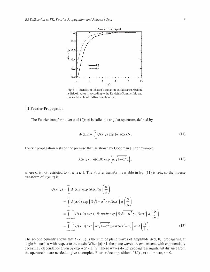
Eqs. (7) and (9) are squared to obtain intensity and are plotted in Fig. 3. The predicted intensities begin to differ appreciably at z/a ≈ 4, where the diffraction angle is χ ≈ 15°. Note that the exactly on-axis intensity of Poisson’s spot doesn’t depend on wavelength because there is no wavelength dependence in the inclination factor. Wavelength dependence enters in the radial intensity distribution, which, for the central region defined by r⊥/a << 1, where r⊥ is the 2-D radius measured from the z axis, can be shown to be [4]

U r z U z

i rz

Jar

( , ) ( , , ) exp⊥⊥ ⊥=

0 0

22

0πλ

πλλz

.

(10)

The first zero of J0 is at 2πar⊥/λz = 2.4, which shows that the diameter of Poisson’s spot is proportional to λ, so the spot’s area and the power contained in it are proportional to λ2.

4. DOING DIFFRACTION WITH FOURIER PROPAGATION

In Section 4.1, I invoke the basic principles of Fourier propagation, and then use these principles in Section 4.2 to derive the RS diffraction integral. For ease of presentation, I address the 2-D diffraction problem: long slits or strips illuminated by plane or cylindrical waves that can be described by U(x, z). In Section 4.1 the generalization to 3-D is obvious; for Section 4.2, it is done in Appendix B.

za

x'

r

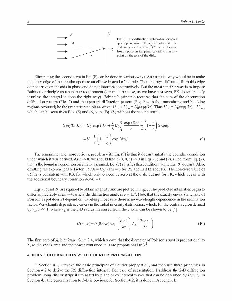
xFig. 2 — The diffraction problem for Poisson’s spot; a plane wave falls on a circular disk. The distance r = (x2 + y2 + z2)1/2 is the distance from a point in the plane of diffraction to a point on the axis of the disk.

RS Diffraction vs FK, Fourier Propagation, and Poisson’s Spot 5

4.1 Fourier Propagation

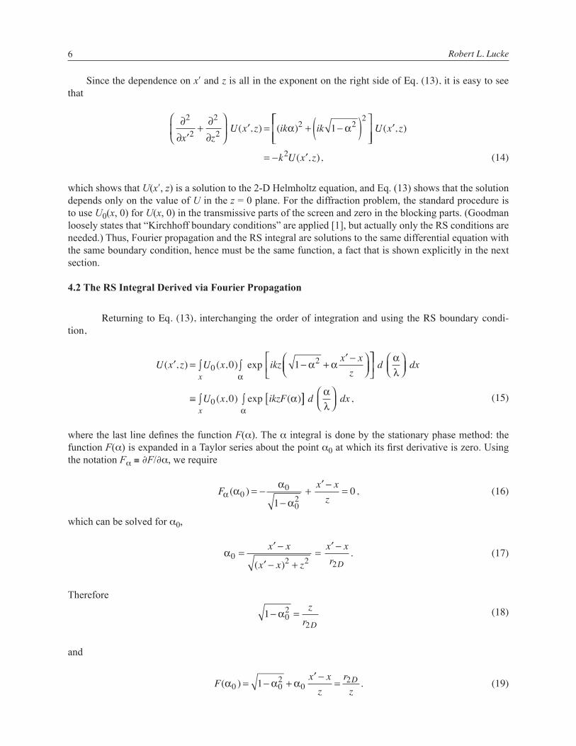
The Fourier transform over x of U(x, z) is called its angular spectrum, defined by

A z U x z ik x dx( , ) ( , ) exp ( ) .α α≡ −

−∞

∞∫

(11)

Fourier propagation rests on the premise that, as shown by Goodman [1] for example,

A z A ik z( , ) ( , ) exp ,α α α= −( )0 1 2

(12)

where α is not restricted to -1 ≤ α ≤ 1. The Fourier transform variable in Eq. (11) is α/λ, so the inverse transform of A(α, z) is

U x z A z ik x d

A

( , ) ( , ) exp ( )

(

′ = ′

=

−∞

∞∫ α α

αλ

αα α ααλ

, ) exp

(

0 1 2ik z ik x d

U

− + ′( )

=

−∞

∞∫

xx ik x dx ik z ik x, ) exp ( ) exp0 1 2− − + ′( )−∞

∞∫ α α α

( , ) exp (

d

U x ik z ik x

αλ

α α

= − + ′ −

−∞

∞∫

0 1 2 xx dxd) .

−∞

∞

−∞

∞∫∫

αλ

(13)

The second equality shows that U(xʹ, z) is the sum of plane waves of amplitude A(α, 0), propagating at angle θ = cos-1α with respect to the x axis. When |α| > 1, the plane waves are evanescent, with exponentially decaying z-dependence given by exp[-(α2 - 1)½z]. These waves do not propagate a significant distance from the aperture but are needed to give a complete Fourier decomposition of U(xʹ, z) at, or near, z = 0.

Fig. 3 — Intensity of Poisson’s spot at on-axis distance z behind a disk of radius a, according to the Rayleigh-Sommerfeld and Fresnel-Kirchhoff diffraction theories.

Robert L. Lucke6

Since the dependence on xʹ and z is all in the exponent on the right side of Eq. (13), it is easy to see that

∂∂ ′

+∂∂

′ = + −( )2

2

2

22 2

21

x zU x z ik ik( , ) ( )α α

′

= − ′

( , )

( , ),

U x z

k U x z2 (14)

which shows that U(xʹ, z) is a solution to the 2-D Helmholtz equation, and Eq. (13) shows that the solution depends only on the value of U in the z = 0 plane. For the diffraction problem, the standard procedure is to use U0(x, 0) for U(x, 0) in the transmissive parts of the screen and zero in the blocking parts. (Goodman loosely states that “Kirchhoff boundary conditions” are applied [1], but actually only the RS conditions are needed.) Thus, Fourier propagation and the RS integral are solutions to the same differential equation with the same boundary condition, hence must be the same function, a fact that is shown explicitly in the next section.

4.2 The RS Integral Derived via Fourier Propagation

Returning to Eq. (13), interchanging the order of integration and using the RS boundary condi-tion,

U x z U x ikzx x

z( , ) ( , ) exp′ = − +

′ −

020 1 α α

≡ [

∫∫α

αλ

α( , ) exp ( )

d dx

U x ikzF

x

0 0 ]]

∫∫ ,d dx

x

αλα

(15)

where the last line defines the function F(α). The α integral is done by the stationary phase method: the function F(α) is expanded in a Taylor series about the point α0 at which its first derivative is zero. Using the notation Fα ≡ ∂F/∂α, we require

Fx x

zα αα

α( ) ,0

0

021

0= −−

+′ −

=

(16)

which can be solved for α0,

α0 2 2 2

=′ −

′ − +=

′ −x x

x x z

x xr D( )

.

(17)

Therefore

1 0

2

2− =α

zr D

(18)

and

F

x xz

rzD( ) .α α α0 0

20

21= − +′ −

=

(19)

RS Diffraction vs FK, Fourier Propagation, and Poisson’s Spot 7

The second derivative of F(α) at α0 is

Frz

Dαα α

α

α

α α( ) .0

02

02

02 3

02 3

23

31

1 1

1

1= −

−−

−= −

−= −

(20)

Since the first-order term vanishes by construction, the Taylor series expansion through second order of F(α) about α0 is

F F F( ) ( ) ( )( ) .α α α α ααα≈ + −0 0 0

212

(21)

A standard Fresnel integral is now written in a form that will be useful below:

exp ( )− −

−

iz

A u u duπ

λ λ02

∞∞

∞∫ =

−,

12

1izAλ

(22)

where A is positive definite.

The integral over α in Eq. (15) can now be evaluated. For ease of notation, drop the α0 argument from Fαα and observe that Fαα = -|Fαα| (Fαα is always negative). Eq. (21) is inserted into the exponent in Eq. (15) to obtain:

exp ( ) exp ( )ikzF ikz Fα α ααα0 021

2[ ] − −

= ( ) −

=

∫ d

ikri

z FD

αλ

λ

α

ααexp

ex

21

21

pp .ikri

rz

rDD D

22 2

12

1( ) −λ

(23)

Therefore

U x z U x ikri

rz

rDD

( , ) ( , ) exp′ = ( ) −0 2

2 20

12

1λ DDx

D

D

dx

iU x

ikrr

∫

=− ( )12

002

22λ

χ( , )exp

cos DDx

dx∫ .

(24)

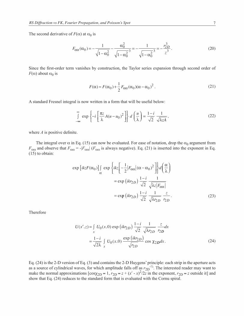
Eq. (24) is the 2-D version of Eq. (3) and contains the 2-D Huygens’ principle: each strip in the aperture acts as a source of cylindrical waves, for which amplitude falls off as r2D

-½. The interested reader may want to make the normal approximations [cosχ2D ≈ 1, r2D ≈ z + (xʹ - x)2/2z in the exponent, r2D ≈ z outside it] and show that Eq. (24) reduces to the standard form that is evaluated with the Cornu spiral.

Robert L. Lucke8

Extending Eq. (24) to the 3-D problem will, first of all, add a dy to the integral. Keeping in mind that all the units of length must cancel out on the right side, inspection of Eq. (24) suggests that the effect of a 3-D calculation is to replace r2D and χ2D by r and χ, to replace cylindrical waves by spherical waves, and to square the factor outside the integral. This intuitive argument is confirmed in detail in Appendix B, with a result, Eq. (B14), that matches the RS form of the diffraction integral given in Eq. (3).

5. CONCLUSION

The fundamental flaw in the FK diffraction integral and the superiority of RS have been demonstrated with exact calculations of the intensity of Poisson’s spot. Fourier propagation has been presented as an alternate means of deriving the diffraction integral. Compared to the usual approach via Green’s theorem, this derivation has the advantage of rendering obvious the proper choice of boundary conditions. It has the disadvantage of requiring knowledge of Fourier propagation and, for the 3-D version, more complicated math, but the 2-D version is not bad and the generalization to 3-D by inspection is intuitively appealing.

As noted in the introduction, the argument has been confined to scalar wave theory, which will not be completely adequate for describing Poisson’s spot in optics for points near the disk. (The contribution of those rays not polarized parallel to the diffracting edge should be multiplied by the sine of the angle between the polarization vector and the direction to the observation point.) But it should be entirely adequate for de-scribing Poisson’s spot in an acoustics experiment because acoustic waves are scalar (pressure) waves. Also, because the wavelength is much longer, diffraction phenomena can be more easily studied in an acoustics than in an optics laboratory. This experiment was done many years ago with somewhat equivocal results [8]. With modern equipment, it should not be particularly difficult to repeat, and could settle the conflict between RS and FK diffraction by direct measurement.

REFERENCES

1. J. W. Goodman, Introduction to Fourier Optics (John Wiley & Sons, New York, 1968), 1st ed., pp. 41-44 and Sec. 3.7.

2. A. Sommerfeld, Lectures on Theoretical Physics, v. 4: Optics (Academic Press, New York, 1954), pp. 198-201 and 211-212.

3. M. Born and E. Wolf, Principles of Optics (Pergamon Press, New York, 1970), pp. 381-382.

4. G.E. Sommargren and H.J. Weaver, “Diffraction of Light by an Opaque Sphere. 1: Description of the Diffraction Pattern,” Appl. Opt. 29, 4646-4657 (1990).

5. E.A. Hovenac, “Fresnel Diffraction by Spherical Obstacles,” Am. J. Phys. 57, 79-84 (1989).

6. J.E. Harvey, J.L. Forgham, and K. Von Bieren, “The Spot of Arago and Its Role in Wavefront Analysis,” Proceedings of SPIE, Vol. 351 – Wavefront Sensing, N. Bareket and C.L. Koliopoulos, eds., Aug. 24 - 25, 1982, San Diego, California, pp. 2-9.

7. H. Osterberg and L.W. Smith, “Closed Solutions of Rayleigh’s Diffraction Integral for Axial Points,” JOSA 51, 1050-1057 (1961).

8. H. Primakoff, M.J. Klein, J.B. Keller, and E.L. Carstensen, “Diffraction of Sound Around a Circular Disk,” J. Acoust. Soc. Am 19, 132-142 (1947).

RS Diffraction vs FK, Fourier Propagation, and Poisson’s Spot 9

Appendix A

THE SOMMERFELD LEMMA

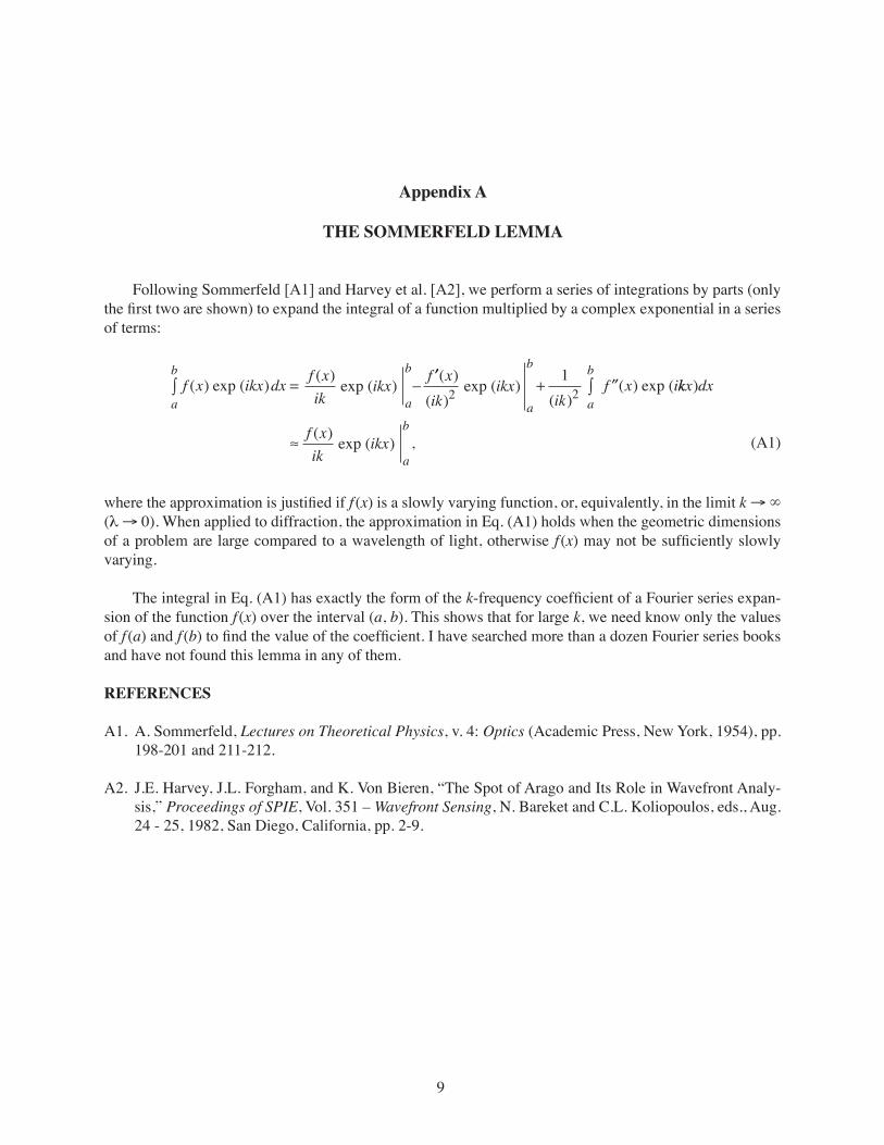
Following Sommerfeld [A1] and Harvey et al. [A2], we perform a series of integrations by parts (only the first two are shown) to expand the integral of a function multiplied by a complex exponential in a series of terms:

f x ikx dx f xik

ikxa

b

a

b

a

b

( ) exp ( ) ( )exp ( )∫ = −

′′ + ′′f xik

ikxik

f x i( )( )

exp ( )( )

( ) exp (2 21

kkx dx

f xik

ikx

a

b

a

b

)

( )exp ( ) ,

∫

≈

(A1)

where the approximation is justified if f (x) is a slowly varying function, or, equivalently, in the limit k → ∞ (λ → 0). When applied to diffraction, the approximation in Eq. (A1) holds when the geometric dimensions of a problem are large compared to a wavelength of light, otherwise f (x) may not be sufficiently slowly varying.

The integral in Eq. (A1) has exactly the form of the k-frequency coefficient of a Fourier series expan-sion of the function f (x) over the interval (a, b). This shows that for large k, we need know only the values of f (a) and f (b) to find the value of the coefficient. I have searched more than a dozen Fourier series books and have not found this lemma in any of them.

REFERENCES

A1. A. Sommerfeld, Lectures on Theoretical Physics, v. 4: Optics (Academic Press, New York, 1954), pp. 198-201 and 211-212.

A2. J.E. Harvey, J.L. Forgham, and K. Von Bieren, “The Spot of Arago and Its Role in Wavefront Analy-sis,” Proceedings of SPIE, Vol. 351 – Wavefront Sensing, N. Bareket and C.L. Koliopoulos, eds., Aug. 24 - 25, 1982, San Diego, California, pp. 2-9.

9

RS Diffraction vs FK, Fourier Propagation, and Poisson’s Spot 11

Appendix B

DERIVING THE RS DIFFRACTION INTEGRAL VIA FOURIER PROPAGATION

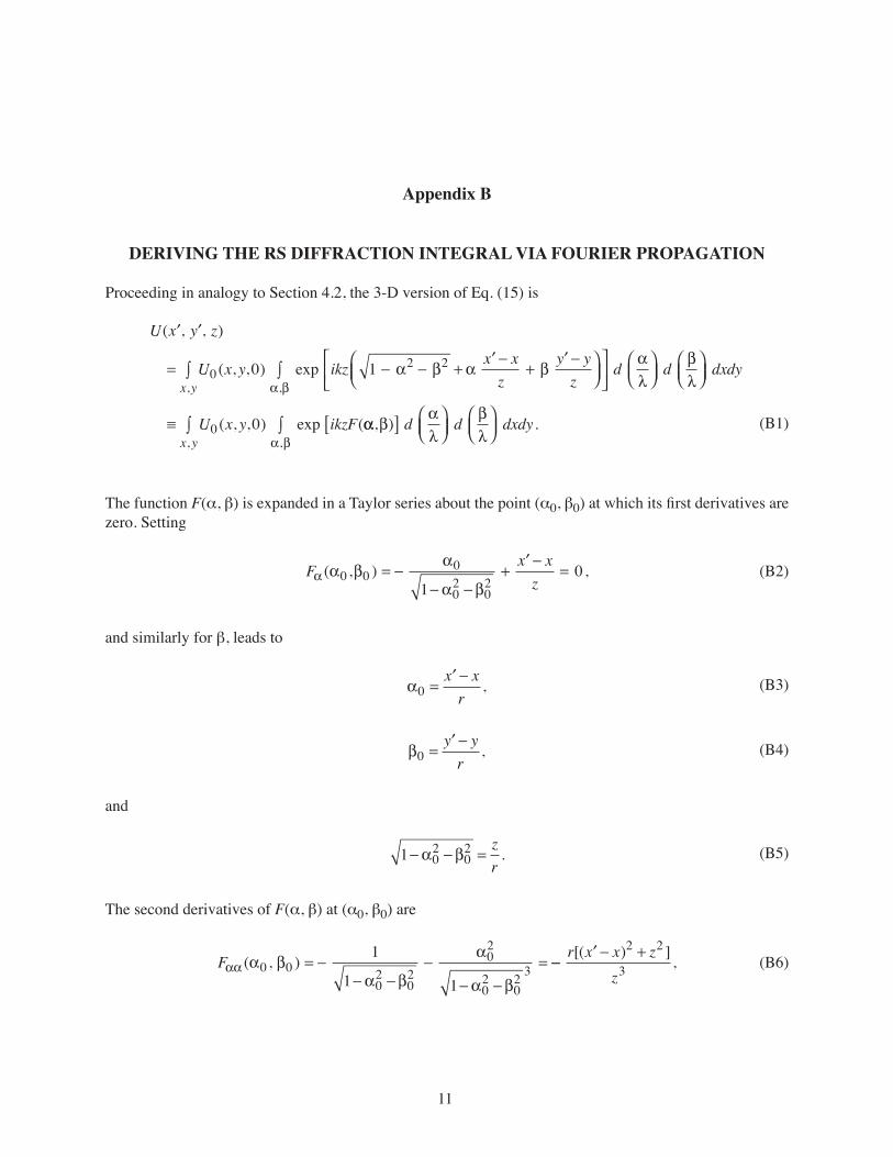
Proceeding in analogy to Section 4.2, the 3-D version of Eq. (15) is

U x y z

U x y ikz

( , , )

( , , ) exp

′ ′

= − − +02 20 1 α β α

,

′ −+

′ −

∫

x xz

y yz

dβαλα β

≡

∫

( , , ) exp (

,d dxdy

U x y ikzF

x y

βλ

0 0 αα βαλ

βλα β

, ) .,,

[ ]

∫∫ d d dxdy

x y (B1)

The function F(α, β) is expanded in a Taylor series about the point (α0, β0) at which its first derivatives are zero. Setting

Fx x

zα α βα

α β( , ) ,0 0

0

02

021

0= −− −

+′ −

=

(B2)

and similarly for β, leads to

α0 =

′ −x xr

,

(B3)

β0 =

′ −y yr

,

(B4)

and

1 0

202− − =α β

zr

.

(B5)

The second derivatives of F(α, β) at (α0, β0) are

Fαα α βα β

α

α β( , )0 0

02

02

02

02

02 3

1

1 1= −

− −−

− −= −−

′ − +[( ) ],

r x x zz

2 2

3

(B6)

11

Robert L. Lucke12

F

r y y zz

ββ α β( , )[( ) ]

,0 0

2 2

3= −′ − +

(B7)

and

Fr x x y

αβ α βα β

α β( , )

( )(0 0

0 0

02

02 3

1= −

− −= −

′ − ′ − yyz

).3

(B8)

The following quantities will be needed below:

F

zr

x xz

y yz

rz

( , )( ) ( )

α βα β

0 00 0= +

′ −+

′ −=

(B9)

and

F F F

rz

αα ββ αβα β α β α β( , ) ( , ) ( , )0 0 0 02

0 0

4− = 44 .

(B10)

The Taylor series expansion through second order of F(α, β) about the point (α0, β0) is

F F F( , ) ( , ) ( , ) ( )α β α β α β α ααα≈ + − +0 0 0 0 021

2112 0 0 0

2

0 0 0

( , ) ( )

( , ) ( ) (

F

F

ββ

αβ

α β β β

α β α α

−

+ − ββ β− 0 ). (B11)

The α and β integrals in Eq. (B1) can now be evaluated. Observe that Fαα = – | Fαα | (Fαα is always nega-tive) and, for ease of notation, drop the (α0, β0) argument from the quantities Fαα, Fββ, and Fαβ. The first, second, and fourth terms in Eq. (B11) are inserted into the exponent in Eq. (B1), and the integral over α is evaluated by completing the square in the exponent (the symbol ± in Eq. (B12) means add and subtract, not add or subtract):

exp ( , ) exp ( )ikzF ikz Fα β α ααα0 0 021

2[ ] − − + FF dαβ

αα α β β

αλ

( )( )

e

− −

=

∫ 0 0

xxp ( ) exp ( )ikrikz

FFF

− − −2

202

αααβ

ααα α (( ) ( ) ( )α α β β β βαβ

αα− − ± −

0 0

2

2 02F

F

=

∫

exp ( ) exp

d

ikrikz F

αλα

2ααβ

ααααβ β α α

2

02

02Fikz

F( ) exp−

− − −FFF

dαβ

ααβ β

αλ

( )−

0

2

= −

∫α

αβ

ααβ βexp ( ) exp ( )ikr

ikz F

F2

2

02

−.

12

1i

z Fλ αα(B12)

RS Diffraction vs FK, Fourier Propagation, and Poisson’s Spot 13

The integral over β in Eq. (B1) can now be carried out by adding the third term in Eq. (B11) to the exponent in Eq. (B12), and again using Fαα = – | Fαα | :

12

12

2−

−i

z Fikr

ikz F

Fexp ( ) exp (

λβ

αα

αβ

ααββ β β

βλββ

β0

20

22

) ( )+ −

=

∫ikz

F d

exp ( ) exp1

21

2−

−−i

z Fikr

ikz F F

λ αα

αα ββ FF

Fdαβ

ααβ β

βλ

2

02

−

( )ββ

αα

αα

αα βλ λ

∫

=− −

exp ( )(

12

1 12

i

z Fikr

i F

z F F ββ αβ

λ

−

= −

F

izr

ikr

2

2

)

exp ( ). (B13)

Eq. (B1) can now be written in the desired form:

U x y zi

U x yz ikr

rx( , , ) ( , , )

exp ( )

,′ ′ = −

λ 0 20yy

x y

dxdy

iU x y

ikrr

∫

∫= − ( , , )exp( )

cos,λ

χ0 0 ddxdy .

(B14)