Embed Size (px)
Citation preview
RAY TRACING FROM A DATA MOVEMENT
PERSPECTIVE
by
Daniel Kopta
A dissertation submitted to the faculty ofThe University of Utah
in partial fulfillment of the requirements for the degree of
Doctor of Philosophy
in
Computer Science
School of Computing
The University of Utah
May 2016

Copyright c� Daniel Kopta 2016
All Rights Reserved

T h e U n i v e r s i t y o f U t a h G r a d u a t e S c h o o l
STATEMENT OF DISSERTATION APPROVAL
The dissertation of Daniel Kopta
has been approved by the following supervisory committee members:
Erik Brunvand , Chair 05/26/2015 Date Approved
AlDQ Davis , Member 05/26/2015 Date Approved
Rajeev Balasubramonian , Member 05/26/2015 Date Approved
Peter Shirley , Member 05/26/2015 Date Approved
Steven Parker , Member 05/26/2015 Date Approved
and by Ross Whitaker , Chair/Dean of
the Department/College/School of Computing
and by David B. Kieda, Dean of The Graduate School.
ABSTRACT
Ray tracing is becoming more widely adopted in o✏ine rendering systems due to its
natural support for high quality lighting. Since quality is also a concern in most real time
systems, we believe ray tracing would be a welcome change in the real time world, but is
avoided due to insu�cient performance. Since power consumption is one of the primary
factors limiting the increase of processor performance, it must be addressed as a foremost
concern in any future ray tracing system designs. This will require cooperating advances
in both algorithms and architecture. In this dissertation I study ray tracing system designs
from a data movement perspective, targeting the various memory resources that are the
primary consumer of power on a modern processor. The result is high performance, low
energy ray tracing architectures.
CONTENTS
ABSTRACT . . . . . . . . . . . . . . . . . . . . . . . . . . . . . . . . . . . . . . . . . . . . . . . . . . . . . . . . iii
LIST OF FIGURES . . . . . . . . . . . . . . . . . . . . . . . . . . . . . . . . . . . . . . . . . . . . . . . . . vi
LIST OF TABLES . . . . . . . . . . . . . . . . . . . . . . . . . . . . . . . . . . . . . . . . . . . . . . . . . . . viii
CHAPTERS
1. INTRODUCTION . . . . . . . . . . . . . . . . . . . . . . . . . . . . . . . . . . . . . . . . . . . . . . . 1
1.1 Thesis . . . . . . . . . . . . . . . . . . . . . . . . . . . . . . . . . . . . . . . . . . . . . . . . . . . . . . . 2
2. BACKGROUND . . . . . . . . . . . . . . . . . . . . . . . . . . . . . . . . . . . . . . . . . . . . . . . . 3
2.1 Graphics Hardware . . . . . . . . . . . . . . . . . . . . . . . . . . . . . . . . . . . . . . . . . . . . . 42.1.1 Parallel Processing . . . . . . . . . . . . . . . . . . . . . . . . . . . . . . . . . . . . . . . . . 52.1.2 Commodity GPUs and CPUs . . . . . . . . . . . . . . . . . . . . . . . . . . . . . . . . . 62.1.3 Ray Tracing Processors . . . . . . . . . . . . . . . . . . . . . . . . . . . . . . . . . . . . . . 92.1.4 Ray Streaming Systems . . . . . . . . . . . . . . . . . . . . . . . . . . . . . . . . . . . . . 10
2.2 Threaded Ray Execution (TRaX) . . . . . . . . . . . . . . . . . . . . . . . . . . . . . . . . . . 112.2.1 Architectural Exploration Procedure . . . . . . . . . . . . . . . . . . . . . . . . . . . 122.2.2 Area E�cient Resource Configurations . . . . . . . . . . . . . . . . . . . . . . . . . . 16
3. RAY TRACING FROM A DATA MOVEMENT PERSPECTIVE . . . . 24
3.1 Ray Tracer Data . . . . . . . . . . . . . . . . . . . . . . . . . . . . . . . . . . . . . . . . . . . . . . . 283.1.1 Treelets . . . . . . . . . . . . . . . . . . . . . . . . . . . . . . . . . . . . . . . . . . . . . . . . . . 29
3.2 Streaming Treelet Ray Tracing Architecture(STRaTA) . . . . . . . . . . . . . . . . . . . . . . . . . . . . . . . . . . . . . . . . . . . . . . . . . . . . 303.2.1 Ray Stream Bu↵ers . . . . . . . . . . . . . . . . . . . . . . . . . . . . . . . . . . . . . . . . . 313.2.2 Traversal Stack . . . . . . . . . . . . . . . . . . . . . . . . . . . . . . . . . . . . . . . . . . . . 333.2.3 Reconfigurable Pipelines . . . . . . . . . . . . . . . . . . . . . . . . . . . . . . . . . . . . . 343.2.4 Results . . . . . . . . . . . . . . . . . . . . . . . . . . . . . . . . . . . . . . . . . . . . . . . . . . 37
4. DRAM . . . . . . . . . . . . . . . . . . . . . . . . . . . . . . . . . . . . . . . . . . . . . . . . . . . . . . . . . 44
4.1 DRAM Behavior . . . . . . . . . . . . . . . . . . . . . . . . . . . . . . . . . . . . . . . . . . . . . . . 454.1.1 Row Bu↵er . . . . . . . . . . . . . . . . . . . . . . . . . . . . . . . . . . . . . . . . . . . . . . . 464.1.2 DRAM Organization . . . . . . . . . . . . . . . . . . . . . . . . . . . . . . . . . . . . . . . . 46
4.2 DRAM Timing and the Memory Controller . . . . . . . . . . . . . . . . . . . . . . . . . . 494.3 Accurate DRAM Modeling . . . . . . . . . . . . . . . . . . . . . . . . . . . . . . . . . . . . . . . 50
5. STREAMING THROUGH DRAM . . . . . . . . . . . . . . . . . . . . . . . . . . . . . . . . 52
5.1 Analysis . . . . . . . . . . . . . . . . . . . . . . . . . . . . . . . . . . . . . . . . . . . . . . . . . . . . . . 545.2 Results . . . . . . . . . . . . . . . . . . . . . . . . . . . . . . . . . . . . . . . . . . . . . . . . . . . . . . . 545.3 Conclusions . . . . . . . . . . . . . . . . . . . . . . . . . . . . . . . . . . . . . . . . . . . . . . . . . . . 57
6. TOOLS AND IMPLEMENTATION DETAILS . . . . . . . . . . . . . . . . . . . . . 58
7. CONCLUSIONS AND FUTURE WORK . . . . . . . . . . . . . . . . . . . . . . . . . . 61
7.1 Shading in STRaTA . . . . . . . . . . . . . . . . . . . . . . . . . . . . . . . . . . . . . . . . . . . . 627.1.1 Ray Bu↵er Overflow . . . . . . . . . . . . . . . . . . . . . . . . . . . . . . . . . . . . . . . . 627.1.2 Shading Pipelines and Streams . . . . . . . . . . . . . . . . . . . . . . . . . . . . . . . . 647.1.3 Storing Shader State . . . . . . . . . . . . . . . . . . . . . . . . . . . . . . . . . . . . . . . . 66
7.2 Conclusion . . . . . . . . . . . . . . . . . . . . . . . . . . . . . . . . . . . . . . . . . . . . . . . . . . . . 67
REFERENCES . . . . . . . . . . . . . . . . . . . . . . . . . . . . . . . . . . . . . . . . . . . . . . . . . . . . . 69
v

LIST OF FIGURES
1.1 Breakdown of energy consumption per frame, averaged over many path tracingbenchmark scenes on the TRaX architecture. . . . . . . . . . . . . . . . . . . . . . . . . . . 2
2.1 Z-Bu↵er Rasterization vs. Ray Tracing. . . . . . . . . . . . . . . . . . . . . . . . . . . . . . . 3
2.2 Baseline TRaX architecture. Left: an example configuration of a single ThreadMultiprocessor (TM) with 32 lightweight Thread Processors (TPs) whichshare caches (instruction I$, and data D$) and execution units (XUs). Right:potential TRaX chip organization with multiple TMs sharing L2 caches [93]. 12
2.3 Test scenes used to evaluate performance for the baseline TRaX architecture. . 13
2.4 L1 data cache performance for a single TM with over-provisioned executionunits and instruction cache. . . . . . . . . . . . . . . . . . . . . . . . . . . . . . . . . . . . . . . . . 17
2.5 E↵ect of shared execution units on issue rate shown as a percentage of totalcycles . . . . . . . . . . . . . . . . . . . . . . . . . . . . . . . . . . . . . . . . . . . . . . . . . . . . . . . . . 18
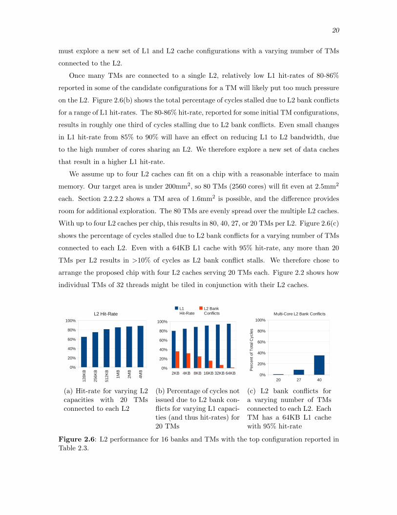
2.6 L2 performance for 16 banks and TMs with the top configuration reported inTable 2.3. . . . . . . . . . . . . . . . . . . . . . . . . . . . . . . . . . . . . . . . . . . . . . . . . . . . . . . 20
3.1 A simplified processor data movement network. Various resources to movedata to the execution unit (XU) include an instruction cache (I$), instructionfetch/decode unit (IF/ID), register file (RF), L1 data cache(D$), L2 sharedcache, DRAM, and Disk. . . . . . . . . . . . . . . . . . . . . . . . . . . . . . . . . . . . . . . . . . . 24
3.2 Treelets are arranged in to cache-sized data blocks. Primitives are stored in aseparate type of “treelet” (red) di↵erentiated from node treelets (blue). . . . . . 32
3.3 Data-flow representation of ray-box intersection. The red boxes at the top arethe inputs (3D vectors), and the red box at the bottom is the output. Edgeweights indicate operand width. . . . . . . . . . . . . . . . . . . . . . . . . . . . . . . . . . . . . 35
3.4 Data-flow representation of ray-triangle intersection using Plucker coordinates [88].The red boxes at the top are the inputs, and the red box at the bottom is theoutput. All edges represent scalar operands. . . . . . . . . . . . . . . . . . . . . . . . . . . . 36
3.5 Benchmark scenes used to evaluate performance for STRaTA and a baselinepathtracer. . . . . . . . . . . . . . . . . . . . . . . . . . . . . . . . . . . . . . . . . . . . . . . . . . . . . . 38
3.6 Performance on three benchmark scenes with varying number of TMs. EachTM has 32 cores. Top graph shows baseline performance and bottom graphshows the proposed technique. Performance plateaus due to the 256GB/sbandwidth limitation. . . . . . . . . . . . . . . . . . . . . . . . . . . . . . . . . . . . . . . . . . . . . 39
3.7 Number of L1 misses (solid lines) for the baseline, and the proposed STRaTAtechnique and stream memory accesses (dashed line) on the three benchmarkscenes. L1 hit rates range from 93% - 94% for the baseline, and 98.5% to 99%for the proposed technique. . . . . . . . . . . . . . . . . . . . . . . . . . . . . . . . . . . . . . . . . 40
3.8 E↵ect of L2 cache size (Baseline) and stream memory size (STRaTA) onmemory system energy for the Sibenik scene. . . . . . . . . . . . . . . . . . . . . . . . . . . 41
3.9 E↵ect of L2 cache size (Baseline) and stream memory size (STRaTA) onmemory system energy for the Vegetation scene. . . . . . . . . . . . . . . . . . . . . . . . 41
3.10 E↵ect of L2 cache size (Baseline) and stream memory size (STRaTA) onmemory system energy for the Hairball scene. . . . . . . . . . . . . . . . . . . . . . . . . . 42
4.1 A small portion of a DRAM mat. A row is read by activating its correspondingwordline, feeding the appropriate bits into the sense amplifiers (S.A.). In thiscase, the four sense amplifiers shown, using internal feedback, make up a smallrow bu↵er. . . . . . . . . . . . . . . . . . . . . . . . . . . . . . . . . . . . . . . . . . . . . . . . . . . . . 45
4.2 Simple DRAM access timing examples showing the processing of two simul-taneous read requests (load A and B). . . . . . . . . . . . . . . . . . . . . . . . . . . . . . . . . 48
5.1 Treelets are arranged in contiguous data blocks targeted as a multiple of theDRAM row size. In this example treelets are constructed to be the sizeof two DRAM rows. Primitives are stored in a separate type of “treelet”di↵erentiated from node treelets, and subject to the same DRAM row sizes. . . 53
5.2 Performance on a selection of benchmark scenes with varying number of TMs.Each TM has 32 cores. Performance plateaus due to DRAM over-utilization. . 57
6.1 Example simtrax profiler output running a basic path tracer. Numbers besidefunction names represent percentage of total execution time. . . . . . . . . . . . . . . 60
7.1 Pseudocode for part of a glass material shader. . . . . . . . . . . . . . . . . . . . . . . . . 63
vii
LIST OF TABLES
2.1 Estimated performance requirements for movie-quality ray traced images at30Hz. . . . . . . . . . . . . . . . . . . . . . . . . . . . . . . . . . . . . . . . . . . . . . . . . . . . . . . . . . 7
2.2 Feature areas and performance for the baseline over-provisioned 1GHz 32-coreTM configuration. In this configuration each core has a copy of every executionunit. . . . . . . . . . . . . . . . . . . . . . . . . . . . . . . . . . . . . . . . . . . . . . . . . . . . . . . . . . . 16
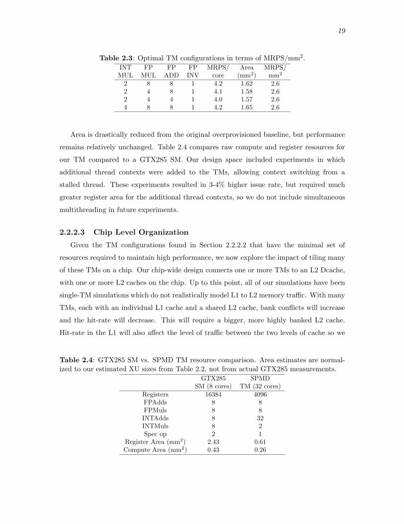
2.3 Optimal TM configurations in terms of MRPS/mm2. . . . . . . . . . . . . . . . . . . . 19
2.4 GTX285 SM vs. SPMD TM resource comparison. Area estimates are nor-malized to our estimated XU sizes from Table 2.2, not from actual GTX285measurements. . . . . . . . . . . . . . . . . . . . . . . . . . . . . . . . . . . . . . . . . . . . . . . . . . 19
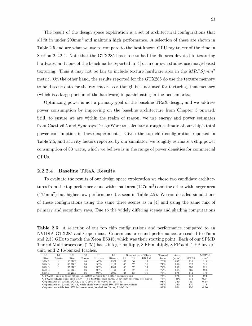
2.5 A selection of our top chip configurations and performance compared to anNVIDIA GTX285 and Copernicus. Copernicus area and performance arescaled to 65nm and 2.33 GHz to match the Xeon E5345, which was theirstarting point. Each of our SPMD Thread Multiprocessors (TM) has 2 integermultiply, 8 FP multiply, 8 FP add, 1 FP invsqrt unit, and 2 16-banked Icaches. 21
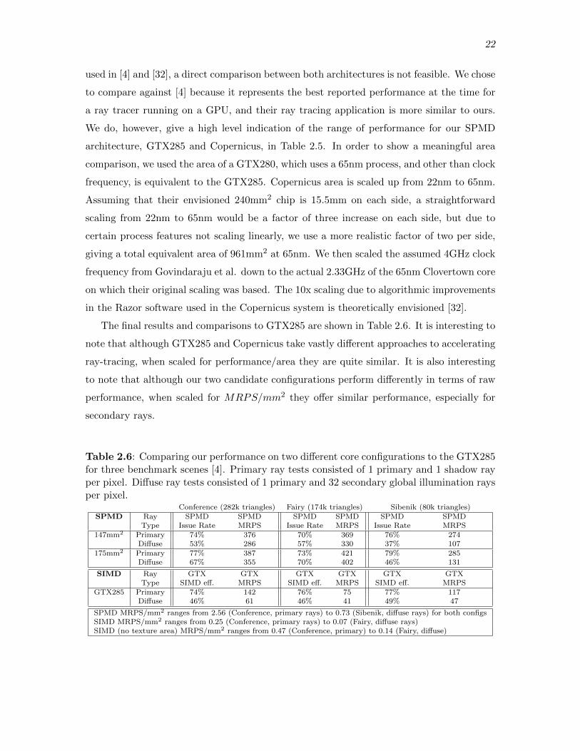
2.6 Comparing our performance on two di↵erent core configurations to the GTX285for three benchmark scenes [4]. Primary ray tests consisted of 1 primary and 1shadow ray per pixel. Di↵use ray tests consisted of 1 primary and 32 secondaryglobal illumination rays per pixel. . . . . . . . . . . . . . . . . . . . . . . . . . . . . . . . . . . . 22
3.1 Resource cost breakdown for a 2560-thread TRaX processor. . . . . . . . . . . . . . . 26
3.2 Instruction cache and register file activation counts for various 3D vectoroperations for general purpose (GP) vs. fused pipeline units. Results are givenas GP / Fused. Energy Di↵ shows the total “Fused” energy as a percentageof “GP”. Activation energies are the estimates used in [51]. . . . . . . . . . . . . . . . 28
3.3 Estimated energy per access in nanojoules for various memories. Estimatesare from Cacti 6.5. . . . . . . . . . . . . . . . . . . . . . . . . . . . . . . . . . . . . . . . . . . . . . . . 42
5.1 DRAM performance characteristics for baseline vs. STRaTA+, where boldsignifies the better performer. Read latency is given in units of GPU clockcycles. STRaTA+ DRAM energy is also shown as a percentage of baselineDRAM energy. For all columns except Row Bu↵er (RB) Hit Rate, lower isbetter. . . . . . . . . . . . . . . . . . . . . . . . . . . . . . . . . . . . . . . . . . . . . . . . . . . . . . . . . 55
7.1 Simulated block transfer from the proposed ray bu↵er sentinel to DRAM.Results are gathered under the same simulated architecture as STRaTA [51].2MB represents half of the ray bu↵er capacity used in [51]. . . . . . . . . . . . . . . 64

CHAPTER 1
INTRODUCTION
Rendering computer graphics is a computationally intensive and power consumptive
operation. Since a very significant portion of our interaction with computers is a visual
process, computer designers have heavily researched more e�cient ways to process graphics.
For application domains such as graphics that perform regular and specialized computations,
and are frequently and continuously active, customized processing units can save tremen-
dous energy and improve performance greatly [24, 58, 39]. As such, almost all consumer
computers built today, including phones, tablets, laptops, and workstations, integrate some
form of graphics processing hardware.
Existing graphics processing units (GPUs) are designed to accelerate Z-bu↵er raster
style graphics [17], a rendering technique used in almost all 3D video games and real-time
applications today. Raster graphics takes advantage of the specialized parallel processing
power of modern graphics hardware to deliver real-time frame rates for increasingly complex
3D environments. Ray-tracing [103] is an alternative rendering algorithm that more natu-
rally supports highly realistic lighting simulation, and is becoming the preferred technique
for generating high quality o✏ine visual e↵ects and cinematics [29]. However, current
ray-tracing systems cannot deliver high quality rendering at the frame rates required by
interactive or real-time applications such as video games [10]. Reaching the level of cinema-
quality rendering in real-time will require at least an order of magnitude improvement
in ray processing throughput. We believe this will require cooperating advances in both
algorithmic and hardware support.
Power is becoming a primary concern of chip manufacturers, as heat dissipation limits
the number of active transistors on high-performance chips, battery life limits usability in
mobile devices, and power costs to run and cool machines is one of the major expenses in a
data center [23, 87, 98]. Much of the energy consumed by a typical modern architecture is
spent in the various memory systems, both on- and o↵-chip, to move data to and from the
computational units. Fetching an operand from main memory can be both slower and three
2
orders of magnitude more energy expensive than performing a floating point arithmetic
operation [23]. In a modern midrange server system, the o↵-chip memory system can
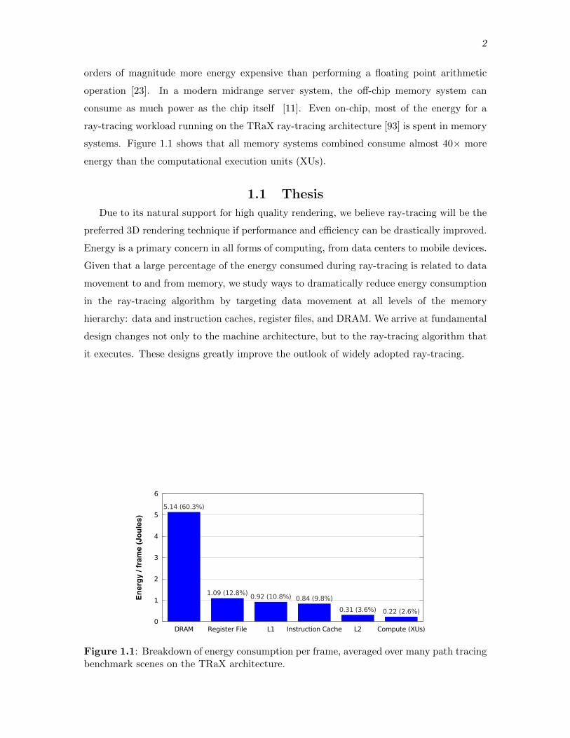
consume as much power as the chip itself [11]. Even on-chip, most of the energy for a
ray-tracing workload running on the TRaX ray-tracing architecture [93] is spent in memory
systems. Figure 1.1 shows that all memory systems combined consume almost 40⇥ more
energy than the computational execution units (XUs).
1.1 ThesisDue to its natural support for high quality rendering, we believe ray-tracing will be the
preferred 3D rendering technique if performance and e�ciency can be drastically improved.
Energy is a primary concern in all forms of computing, from data centers to mobile devices.
Given that a large percentage of the energy consumed during ray-tracing is related to data
movement to and from memory, we study ways to dramatically reduce energy consumption
in the ray-tracing algorithm by targeting data movement at all levels of the memory
hierarchy: data and instruction caches, register files, and DRAM. We arrive at fundamental
design changes not only to the machine architecture, but to the ray-tracing algorithm that
it executes. These designs greatly improve the outlook of widely adopted ray-tracing.
0
1
2
3
4
5
6
DRAM Register File L1 Instruction Cache L2 Compute (XUs)
En
erg
y / f
ram
e (J
ou
les)
5.14 (60.3%)
1.09 (12.8%) 0.92 (10.8%) 0.84 (9.8%)0.31 (3.6%) 0.22 (2.6%)
Figure 1.1: Breakdown of energy consumption per frame, averaged over many path tracingbenchmark scenes on the TRaX architecture.
CHAPTER 2
BACKGROUND
Interactive computer graphics today is dominated by extensions to Catmull’s original
Z-bu↵er rasterization algorithm [17]. The basic operation of this type of rendering is to
project 3D primitives (usually triangles) on to the 2D screen. This 2D representation of the
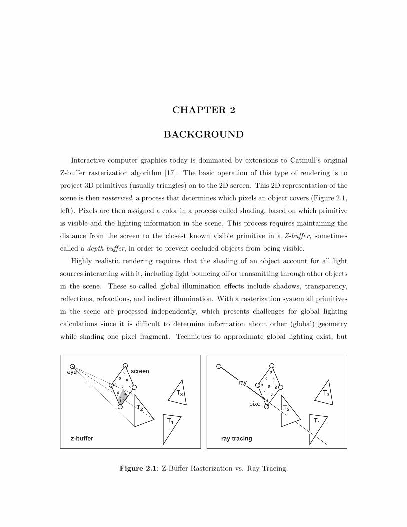
scene is then rasterized, a process that determines which pixels an object covers (Figure 2.1,
left). Pixels are then assigned a color in a process called shading, based on which primitive
is visible and the lighting information in the scene. This process requires maintaining the
distance from the screen to the closest known visible primitive in a Z-bu↵er, sometimes
called a depth bu↵er, in order to prevent occluded objects from being visible.
Highly realistic rendering requires that the shading of an object account for all light
sources interacting with it, including light bouncing o↵ or transmitting through other objects
in the scene. These so-called global illumination e↵ects include shadows, transparency,
reflections, refractions, and indirect illumination. With a rasterization system all primitives
in the scene are processed independently, which presents challenges for global lighting
calculations since it is di�cult to determine information about other (global) geometry
while shading one pixel fragment. Techniques to approximate global lighting exist, but
Figure 2.1: Z-Bu↵er Rasterization vs. Ray Tracing.

4
can have shortcomings in certain situations, and combining them in to a full system is a
daunting task.
Ray-tracing is an alternative rendering algorithm in which the basic operation used to
determine visibility and lighting is to simulate a path of light. For each pixel, a ray is
generated by the camera and sent in to the scene (Figure 2.1, right). The nearest geometry
primitive intersected by that ray is found to determine which object is visible through
that pixel. The color of the pixel (shading) is then computed by creating new rays, either
bouncing o↵ the object (reflection and indirect illumination), transmitting through the
object (transparency), or emitted from the light source (direct lighting and shadows). The
direction and contribution of these so-called secondary rays is determined by the physical
properties of light and materials. Secondary rays are processed through the scene in the
same way as camera rays to determine the closest object hit, and the shading process is
continued recursively. This process directly simulates the transport of light throughout the
virtual scene and naturally produces photo-realistic images.
The process of determining which closest geometry primitive a ray intersects is referred
to as traversal and intersection. In order to avoid the intractable problem of every ray
checking for intersection with every primitive, an acceleration structure is built around the
geometry that allows for quickly culling out large portions of the scene and finding a much
smaller set of geometry the ray is likely to intersect. These structures are typically some
form of hierarchical tree in which each child subtree contains a smaller, more localized
portion of the scene.
Due to the independent nature of triangles in Z-bu↵er rendering, it is trivial to parallelize
the process on many triangles simultaneously. Existing GPUs stream all geometry primi-
tives through the rasterization pipeline using wide parallelism techniques to achieve truly
remarkable performance. Ray-tracing is also trivial to parallelize, but in a di↵erent way:
individual rays are independent and can be processed simultaneously. Z-bu↵er rendering
is generally much faster than ray-tracing for producing a passable image, partly due to
the development of custom hardware support over multiple decades. On the other hand
ray-tracing can provide photo-realistic images much more naturally, and has recently become
feasible as a real-time rendering method on existing and proposed hardware.
2.1 Graphics HardwareThe basic design goal of graphics hardware is to provide massive parallel processing
power. To achieve this, GPUs do away with features of a small set of complex cores in favor
of a vastly greater number of cores, but of a much simpler architecture. These cores often

5
run at a slower clock rate than general purpose cores, but make up for it in the parallelism
enabled by their larger numbers. Since GPUs target a specific application domain (graph-
ics), many general purpose features are not needed, although recent generations of GPUs
are beginning to support more general purpose programmability, particularly for massively
parallel applications.
2.1.1 Parallel Processing
Most processing workloads exhibit some form of parallelism, i.e., there are independent
portions of work that can be performed simultaneously since they don’t a↵ect each other.
There are many forms of parallelism, but we will focus on two of them: data-level parallelism
and task-level parallelism. Z-bu↵er rendering exhibits data parallelism because it performs
the exact same computation on many di↵erent pieces of data (the primitives). Ray-tracing
exhibits task parallelism since traversing a ray through the acceleration structure can require
a di↵erent set of computations per ray (task), but rays can be processed simultaneously.
There are multiple programming models and architectural designs to support these types
of parallelism. Algorithms can be carefully controlled or modified to better match a
certain parallelism model, to varying degrees of success, but there are important benefits
and drawbacks when considering processing and programming models. Some of the basic
architectural models for supporting parallelism include:
Single Instruction, Multiple Data (SIMD)
This is the basic architectural model that supports data-level parallelism. A SIMD
processor fetches and executes one atom of work (instruction) and performs that
operation on more than one set of data operands in parallel. From a hardware
perspective, SIMD is perhaps the simplest way to achieve parallelism since only the
execution units and register file must be replicated. The cost of fetching and decoding
an instruction can be amortized over the width of the data. SIMD processors have
varying data width, typically ranging from 4 to 32. An N-wide SIMD processor
can potentially improve performance by a factor of N, but requires high data-level
parallelism.
Single Instruction, Multiple Thread (SIMT)
A term introduced by NVIDIA, SIMT [55] extends the SIMD execution model to
include the construct of multiple threads. A SIMT processor manages the state of
multiple execution threads (or tasks) simultaneously, and can select which thread(s)
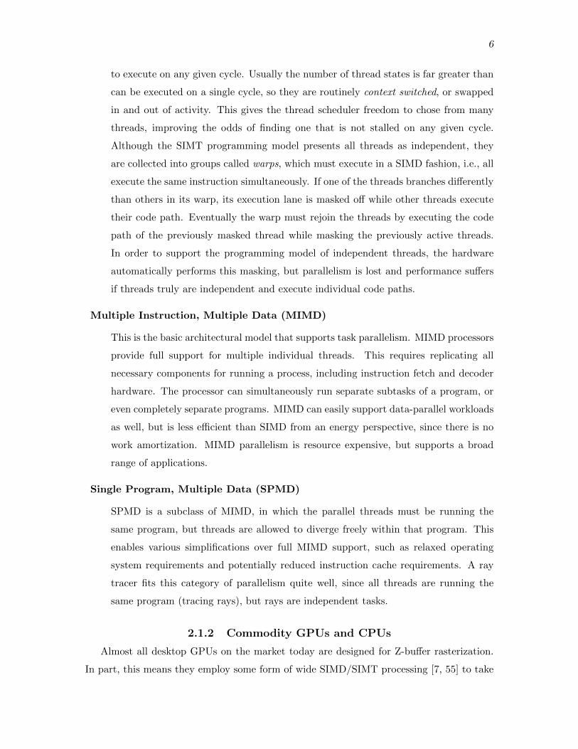
6
to execute on any given cycle. Usually the number of thread states is far greater than
can be executed on a single cycle, so they are routinely context switched, or swapped
in and out of activity. This gives the thread scheduler freedom to chose from many
threads, improving the odds of finding one that is not stalled on any given cycle.
Although the SIMT programming model presents all threads as independent, they
are collected into groups called warps, which must execute in a SIMD fashion, i.e., all
execute the same instruction simultaneously. If one of the threads branches di↵erently
than others in its warp, its execution lane is masked o↵ while other threads execute
their code path. Eventually the warp must rejoin the threads by executing the code
path of the previously masked thread while masking the previously active threads.
In order to support the programming model of independent threads, the hardware
automatically performs this masking, but parallelism is lost and performance su↵ers
if threads truly are independent and execute individual code paths.
Multiple Instruction, Multiple Data (MIMD)
This is the basic architectural model that supports task parallelism. MIMD processors
provide full support for multiple individual threads. This requires replicating all
necessary components for running a process, including instruction fetch and decoder
hardware. The processor can simultaneously run separate subtasks of a program, or
even completely separate programs. MIMD can easily support data-parallel workloads
as well, but is less e�cient than SIMD from an energy perspective, since there is no
work amortization. MIMD parallelism is resource expensive, but supports a broad
range of applications.
Single Program, Multiple Data (SPMD)
SPMD is a subclass of MIMD, in which the parallel threads must be running the
same program, but threads are allowed to diverge freely within that program. This
enables various simplifications over full MIMD support, such as relaxed operating
system requirements and potentially reduced instruction cache requirements. A ray
tracer fits this category of parallelism quite well, since all threads are running the
same program (tracing rays), but rays are independent tasks.
2.1.2 Commodity GPUs and CPUs
Almost all desktop GPUs on the market today are designed for Z-bu↵er rasterization.
In part, this means they employ some form of wide SIMD/SIMT processing [7, 55] to take

7
advantage of the data-parallel nature of Z-bu↵er graphics. To give one example, the GeForce
GTX 980 high-end NVIDIA GPU ships with 64 streaming multiprocessors (SM), each with
a 32-wide SIMD execution unit, for a total of 2048 CUDA cores [70], and a tremendous 4.6
teraflops of peak processing throughput.
Desktop CPUs are primarily multi-core MIMD designs in order to support a wide range
of applications and multiple unrelated processes simultaneously. Individual CPU threads are
typically significantly faster than GPU threads, but overall provide less parallel processing
power. AMD eventually introduced SIMD extensions to the popular x86 instruction set
called 3DNow! [6], which adds various 4-wide SIMD instructions. Similarly, Intel introduced
its own streaming SIMD extensions (SSE) [42], and later the improved 8-wide AVX instruc-
tions [43]. This hybrid MIMD/SIMD approach results in multiple independent threads, each
capable of vector data instruction issue. Intel’s Xeon Phi accelerator takes this approach
to the extreme, with up to 61 MIMD cores, each with a 16-wide SIMD unit, presenting an
intriguing middle ground for a ray-tracing platform.
Current ray-tracing systems are still at least an order of magnitude short in performance
for rendering modest scenes at cinema quality, resolution, and frame rate. Table 2.1
estimates the rays/second performance required for real-time movie-quality ray-tracing
based on movie test renderings [28]. Existing consumer ray-tracing systems can achieve up
to a few hundred million rays per second [5, 102].
2.1.2.1 Ray Tracing on CPUs
Researchers have been developing ray-tracing performance optimizations on CPUs for
many years. Historically, the CPU made for a better target than GPUs, partly due to
the lack of programmability of early commercial GPU hardware. In the past, the intensive
computational power required for ray-tracing was far more than a single CPU could deliver,
but interactivity was possible through parallelizing the workload on a large shared memory
cluster with many CPUs [74]. Around the same time, SSE was introduced, potentially
quadrupling the performance of individual CPU cores, but also requiring carefully mapping
the ray-tracing algorithm to use vector data instructions.
Table 2.1: Estimated performance requirements for movie-quality ray traced images at30Hz.
display type pixels/frame rays/pixel million rays/frame million rays/sec needed
HD resolution 1920x1080 50 - 100 104 - 208 3,100-6,20030” Cinema display 2560x1600 50 - 100 205-410 6,100-12,300

8
Wald et al. collect rays into small groups called packets [101]. These packets of rays
have a common origin, and hopefully similar direction, making them likely to take the same
path through an acceleration structure, and intersect the same geometry. This coherence
among rays in a packet exposes SIMD parallelism opportunities in the form of performing
traversal or intersection operations on multiple (four in the case of SSE) rays simultaneously.
Processing rays in coherent groups also has the e↵ect of amortizing the cost of fetching scene
data across the width of the packet, resulting in reduced memory tra�c.
One of the biggest challenges of a packetized ray tracer is finding groups of rays that
are coherent. Early systems simply used groups of primary rays through nearby pixels,
and groups of point-light shadow rays from nearby shading points. One of the most
important characteristics of ray-tracing is its ability to compute global illumination e↵ects,
which usually require intentionally incoherent (randomized) rays, making it di�cult to form
coherent packets for any groups of rays other than primary camera rays. When incoherent
rays within a packet require di↵erent traversal paths, the packet must be broken apart
into fewer and fewer active rays, losing the intended benefits altogether. Boulos et al. [12]
explore improved packet assembly algorithms, finding coherence among incoherent global
illumination rays. Boulos et al. [13] further improve upon this by dynamically restructuring
packets on the fly, better handling extremely incoherent rays, such as those generated by
path tracing [47].
Despite all e↵orts to maintain coherent ray packets, it is sometimes simply not possible.
An alternative to processing multiple rays simultaneously is to process a single ray through
multiple traversal or intersection steps simultaneously. Since SIMD units are typically at
least 4-wide on CPUs, this favors wide-branching trees in the acceleration structure [27, 99].
A combination of ray packets and wide trees has proven to be quite advantageous, enabling
high SIMD utilization in situations both with and without high ray coherence [8]. Utilizing
these techniques, Intel’s Embree engine [102] can achieve an impressive hundreds of millions
of rays per second when rendering scenes with complex geometry and shading.
2.1.2.2 Ray Tracing on GPUs
As GPUs became more programmable, their parallel compute power made them an
obvious target for ray-tracing. Although still limited in programmability at the time, Purcell
et al. developed the first full GPU ray tracer using the fragment shader as a programmable
portion of the existing graphics pipeline [79]. Their system achieved performance (rays/sec)
similar to or higher than cutting edge CPU implementations at the time [100]. GPUs would
become more supportive of programmable workloads with the advent of CUDA [71] and

9
OpenCL [96], and researchers quickly jumped on the new capabilities with packetized traver-
sal of sophisticated acceleration structures, enabling the rendering of massive models [34].
Aila et al. [4] note that most GPU ray-tracing systems were dramatically underutilizing
the available compute resources, and carefully investigate ray traversal as it maps to GPU
hardware. They indicate that ray packets do not perform well on extremely wide (32 in their
case) SIMD architectures, and instead provide thoroughly investigated and highly optimized
per-ray traversal kernels. With slight updates to take advantage of newer architectures,
their kernels can process hundreds of millions of di↵use rays per second [5]. Still, the SIMD
utilization (percentage of active compute units) is usually less than half [4], highlighting the
di�culties caused by the divergent code paths among incoherent rays.
NVIDIA’s OptiX [75] is a ray-tracing engine and API that provides users the tools to
assemble a full, custom ray tracer without worrying about the tricky details of GPU code
optimization. OptiX provides high performance kernels including acceleration structure
generation and traversal, which can be combined with user-defined kernels for, e.g. shading,
by an optimizing compiler. Although flexible and programmable, OptiX is able to achieve
performance close to the highly tuned ray tracers in [4].
2.1.3 Ray Tracing Processors
Despite the increasing programmability of today’s GPUs, many argue that custom ray-
tracing architectural features are needed to achieve widespread adoption, whether in the
form of augmentations to existing GPUs or fully custom designs.
One of the early e↵orts to design a fully custom ray-tracing processor was SaarCOR [84,
85], later followed by Ray Processing Unit (RPU) [106, 105]. SaarCOR and RPU are
custom hard-coded ray-tracing processors, except RPU has a programmable shader. Both
are implemented and demonstrated on an FPGA and require that a kd-tree be used. The
programmable portion of the RPU is known as the Shading Processor (SP), and consists
of four 4-way vector cores running in SIMD mode with 32 hardware threads supported on
each of the cores. Three caches are used for shader data, kd-tree data, and geometry data.
Cache coherence is quite good for primary rays and adequate for secondary rays. With an
appropriately described scene (using kd-trees and triangle data encoded with unit-triangle
transformations) the RPU can achieve impressive frame rates for the time, especially when
extrapolated to a potential CMOS ASIC implementation [105]. The fixed-function nature
of SaarCOR and RPU provides very high performance at a low energy cost, but limits their
usability.

10
On the opposite end of the spectrum, the Copernicus approach [31] attempts to leverage
existing general purpose x86 cores in a many-core organization with special cache and mem-
ory interfaces, rather than developing a specialized core specifically for ray-tracing. As a
result, the required hardware may be over-provisioned, since individual cores are not specific
to ray-tracing, but using existing core blocks improves flexibility and saves tremendous
design, validation, and fabrication costs. Achieving real-time rendering performance on
Copernicus requires an envisioned tenfold improvement in software optimizations.
The Mobile Ray Tracing Processor (MRTP) [49] recognizes the multiphase nature of
ray-tracing, and provides reconfigurability of execution resources to operate as wide SIMT
scalar threads for portions of the algorithm with nondivergent code paths, or as a narrower
SIMT thread width, but with each thread operating on vector data for portions of the
algorithm with divergent code paths. Each MRTP reconfigurable stream multiprocessor
(RSMP) can operate as 12-wide SIMT scalar threads, or 4-wide SIMT vector threads.
Running in the appropriate configuration for each phase of the algorithm helps reduce the
underutilization that SIMT systems can su↵er due to branch divergence. This improves
performance, and as a side-e↵ect, reduces energy consumption due to decreased leakage
current from inactive execution units. This reconfigurability is similar in spirit to some of
our proposed techniques (Section 7.1.2).
Nah et al. present the Traversal and Intersection Engine (T&I) [65], a fully custom
ray tracing processor with fixed-function hardware for an optimized traversal order and
tree layout, as well as intersection. This is combined with programmable shader support,
similar to RPU [106]. T&I also employs a novel ray accumulation unit which bu↵ers rays
that incur cache misses, helping to hide high latency memory accesses. T&I was later
improved to be used as the GPU portion of a hybrid CPU/GPU system [64]. The primitive
intersection procedure and acceleration structure builder is modified so that every primitive
is enclosed with an axis-aligned bounding-box (AABB), and the existing AABB intersection
unit required for tree traversal is reused to further cull primitive intersections. Essentially,
this has the e↵ect of creating shallower trees that are faster to construct.
2.1.4 Ray Streaming Systems
Data access patterns can have a large impact on performance (see Chapters 3 and 4).
In an e↵ort to make the ray-tracing memory access patterns more e�cient, recent work has
proposed significantly modifying the ray-tracing algorithm. Navratil et al. [67] and Aila et
al.[2] identify portions of the scene data called treelets, which can be grouped together and
fill roughly the capacity of the cache. Rays are then dynamically scheduled for processing

11
based on which group they are in, allowing rays that access similar regions of data to share
the costs associated with accessing that data. This drastically improves cache hit rates,
thus reducing the very costly o↵-chip memory tra�c. The tradeo↵ is that rays must be
bu↵ered for delayed processing, requiring saved ray state, and complicating the algorithm.
We use a similar technique in [50] (Section 3.2).
Gribble and Ramani [33, 82] group rays together by applying a series of filters to a large
set of rays, placing them into categories based on certain properties, e.g., ray type (shadow
or primary), the material hit, whether the ray is active or not, which nodes a ray has
entered, etc. Although their goal was to improve SIMD e�ciency by finding large groups
of rays performing the same computation, it is likely the technique will also improve data
access coherence. Furthermore, by using a flexible multiplexer-driven interconnect, data can
be e�ciently streamed between execution resources, avoiding the register file when possible
and reducing power consumption. We use similar techniques in Section 7.1.2.
Keely [48] reexamines acceleration structure layout, and significantly reduces the numer-
ical precision required for traversal computations. Lower-precision execution units can be
much smaller and more energy e�cient, allowing for many of them to be placed in a small
die area. Keely builds on recent treelet techniques, adding reduced-precision fixed-function
traversal units to an existing high-end GPU, resulting in incredibly high (reduced-precision)
operations per second, kept fed with data by an e�cient data streaming model. The reported
performance is very impressive, at greater than one billion rays per second. Reduced
precision techniques like those used in [48] are independent of treelet/streaming techniques,
and could be applied to to the work proposed in Chapter 3.
2.2 Threaded Ray Execution (TRaX)TRaX is a custom ray-tracing architecture designed from the ground up [52, 93, 94]. The
basic design philosophy behind TRaX aims to tile as many thread processors as possible
on to the chip for massive parallel processing of independent rays. Thread processors are
kept very simple, their small size permitting many of them in a given die area. To achieve
this, each thread only has simple thread state, integer, issue, and control logic. Large or
expensive resources are not replicated for each thread. These larger units—floating point
arithmetic, instruction caches, and data caches—are shared by multiple thread processors,
relying on the assumption that not all threads will require a shared resource at the same
time. This assumption is supported by a SPMD parallelism model, in which threads can

12
diverge independently through execution of the code, naturally requiring di↵erent resources
at di↵erent times.
Figure 2.2 shows an example block diagram of a TRaX processor. The basic architecture
is a collection of simple, in-order, single-issue integer thread processors (TPs) configured
with general purpose registers and a small local memory. The generic TRaX thread
multiprocessor (TM) aggregates a number of TPs which share more expensive resources.
The specifics of the size, number, and configuration of the processor resources are variable.
Simtrax [38] is a cycle-accurate many-core GPU simulator supported by a powerful
compiler toolchain and API [92]. Simtrax allows for the customization of nearly all
components of the processor, including cache and memory capacities and banking, cache
policies, execution unit mix and connectivity, and even the addition of custom units or
memories. Simtrax is open source, so the overall architecture, ISA, and API are all adaptable
as needed. We investigate a broad design space of configurations through simulation and
attempt to find optimal designs in terms of performance per die area.
2.2.1 Architectural Exploration Procedure
The main architectural challenge in the design of a ray-tracing processor is to provide
support for the many independent rays that must be computed for each frame. Our
approach is to optimize single-ray SPMD performance. This approach can ease application
TMs TMs
L2TMs TMs
L2TMs TMs
L2TMs TMs
L2
L1
D$
XUs
I$ I$TPs TPs
Figure 2.2: Baseline TRaX architecture. Left: an example configuration of a singleThread Multiprocessor (TM) with 32 lightweight Thread Processors (TPs) which sharecaches (instruction I$, and data D$) and execution units (XUs). Right: potential TRaXchip organization with multiple TMs sharing L2 caches [93].
13
development by reducing the need to orchestrate coherent ray bundles and execution kernels
compared to a SIMD/SIMT ray tracer. To evaluate our design choices, we compare our
architecture to the best known SIMT GPU ray tracer at the time [4].
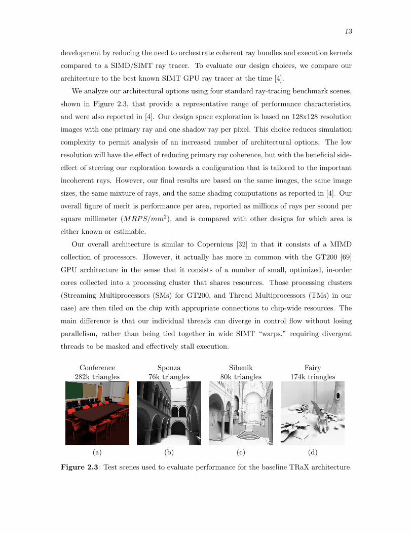
We analyze our architectural options using four standard ray-tracing benchmark scenes,
shown in Figure 2.3, that provide a representative range of performance characteristics,
and were also reported in [4]. Our design space exploration is based on 128x128 resolution
images with one primary ray and one shadow ray per pixel. This choice reduces simulation
complexity to permit analysis of an increased number of architectural options. The low
resolution will have the e↵ect of reducing primary ray coherence, but with the beneficial side-
e↵ect of steering our exploration towards a configuration that is tailored to the important
incoherent rays. However, our final results are based on the same images, the same image
sizes, the same mixture of rays, and the same shading computations as reported in [4]. Our
overall figure of merit is performance per area, reported as millions of rays per second per
square millimeter (MRPS/mm
2), and is compared with other designs for which area is
either known or estimable.
Our overall architecture is similar to Copernicus [32] in that it consists of a MIMD
collection of processors. However, it actually has more in common with the GT200 [69]
GPU architecture in the sense that it consists of a number of small, optimized, in-order
cores collected into a processing cluster that shares resources. Those processing clusters
(Streaming Multiprocessors (SMs) for GT200, and Thread Multiprocessors (TMs) in our
case) are then tiled on the chip with appropriate connections to chip-wide resources. The
main di↵erence is that our individual threads can diverge in control flow without losing
parallelism, rather than being tied together in wide SIMT “warps,” requiring divergent
threads to be masked and e↵ectively stall execution.
Conference282k triangles
(a)
Sponza76k triangles
(b)
Sibenik80k triangles
(c)
Fairy174k triangles
(d)
Figure 2.3: Test scenes used to evaluate performance for the baseline TRaX architecture.
14
The lack of synchrony between ray threads reduces resource sharing conflicts between
the cores and reduces the area and complexity of each core. With a shared multibanked
Icache, the cores quickly reach a point where they are each accessing a di↵erent bank, and
shared execution unit conflicts can be similarly reduced.
In order to hide the high latency of memory operations in graphics workloads, GPUs
maintain many threads that can potentially issue an instruction while another thread is
stalled. This approach involves sharing a number of thread states per core, only one of which
can attempt to issue on each cycle. Given that the largest component of TRaX’s individual
thread processor is its register file, adding the necessary resources for an extra thread state
is tantamount to adding a full thread processor. Thus, in order to sustain high instruction
issue rate, we add more full thread processors as opposed to context switching between
thread states. While GPUs can dynamically schedule more or fewer threads based on the
number of registers the program requires [56], the TRaX approach is to allocate a minimal
fixed set of registers per thread. The result is a di↵erent ratio of registers to execution
resources for the cores in our TMs compared to a typical GPU. We rely on asynchrony to
sustain a high issue rate to our heavily shared resources, which enables simpler cores with
reduced area over a fully provisioned processor.
Our exploration procedure first defines an unrealistic, exhaustively-provisioned SPMD
multiprocessor as a starting point. This serves as an upper bound on raw performance, but
requires an unreasonably large chip area. We then explore various multibanked Dcaches and
shared Icaches using Cacti v6.5 [63] to provide area and latency estimates for the various
configurations. Next, we consider sharing large execution units which are not heavily used,
in order to reduce area with a minimal performance impact. Finally we explore a chip-wide
configuration that uses shared L2 caches for a number of TMs.
To evaluate this architectural exploration, we use a simple test application written
in C++, compiled with our custom LLVM [19] backend. This application can be run
as a simple ray tracer with ambient occlusion, or as a path tracer which enables more
detailed global illumination e↵ects using Monte-Carlo sampled Lambertian shading [89]
which generates more incoherent rays. Our ray tracer supports fully programmable shading
and texturing and uses a bounding volume hierarchy acceleration structure. In this work
we use the same shading techniques as in [4], which do not include texturing.
2.2.1.1 Thread Multiprocessor (TM) Design
Our baseline TM configuration is designed to provide an upper bound on the thread
issue rate. Because we have more available details of their implementation, our primary
15
comparison is against the NVIDIA GTX285 [4] of the GT200 architecture family. The
GT200 architecture operates on 32-thread SIMT “warps.”
The “SIMD e�ciency” metric is defined in [4] to be the percentage of SIMD threads
that perform computations. Note that some of these threads perform speculative branch
decisions which may perform useless work, but this work is counted as e�cient. In our
architecture the equivalent metric is thread issue rate. This is the average number of
independent cores that can issue an instruction on each cycle. These instructions always
perform useful work. The goal is to have thread issue rates as high or higher than the SIMD
e�ciency reported on highly optimized SIMD code. This implies an equal or greater level
of parallelism, but with more flexibility.
We start with 32 cores in a TM to be comparable to the 32-thread warp in a GT200 SM.
Each core processor has 128 registers, issues in order, and employs no branch prediction.
To discover the maximum possible performance achievable, each initial core will contain
all of the resources that it can possibly utilize. In this configuration, the data caches are
overly large (enough capacity to entirely fit the dataset for two of our test scenes, and still
unrealistically large for the others), with one bank per core. There is one execution unit
(XU) of each type available for every core. Our ray-tracing code footprint is relatively
small, which is typical for ray tracers (ignoring custom artistic material shaders) [30, 89]
and is similar in size to the ray tracer evaluated in [4]. Hence the Icache configurations
are relatively small and therefore fast enough to service two requests per cycle at 1GHz
according to Cacti v6.5 [63], so 16 instruction caches are su�cient to service the 32 cores.
This configuration provides an unrealistic best-case issue rate for a 32-core TM. Table 2.2
shows the area of each major component in a 65nm process, and the total area for a 32-core
TM, sharing the multibanked Dcache and the 16 single-banked Icaches. Memory area
estimates are from Cacti v6.51.
Memory latency is also based on Cacti v6.5: 1 cycle to L1, and 3 cycles to L2. XU
area estimates are based on synthesized versions of the circuits using Synopsys Design-
Ware/Design Compiler and a commercial 65nm CMOS cell library. These execution unit
area estimates are conservative, as a custom-designed execution unit would certainly have
smaller area. All cells are optimized by Design Compiler to run at 1GHz and multicycle
cells are fully pipelined. The average core issue rate is 89%, meaning that an average of 28.5
cores are able to issue on every cycle. The raw performance of this configuration is very
1We note that Cacti v6.5 has been specifically enhanced to provide more accurate size estimates thanprevious versions for relatively small caches of the type we are proposing.

16
Table 2.2: Feature areas and performance for the baseline over-provisioned 1GHz 32-coreTM configuration. In this configuration each core has a copy of every execution unit.
Unit Area Cycles Total Area(mm2) (mm2)
4MB Dcache (32 banks) 1 33.54KB Icaches 0.07 1 1.12128x32 RF 0.019 1 0.61FP InvSqrt 0.11 16 3.61Int Multiply 0.012 1 0.37FP Multiply 0.01 2 0.33FP Add/Sub 0.003 2 0.11Int Add/Sub 0.00066 1 0.021FP Min/Max 0.00072 1 0.023Total 39.69
Avg thread issue MRPS/core MRPS/mm2
89% 5.6 0.14
good, but the area is huge. The next step is to reduce core resources to save area without
sacrificing performance. With reduced area the MRPS/mm
2 increases and provides an
opportunity to tile more TMs on a chip.
2.2.2 Area E�cient Resource Configurations
We now consider constraining caches and execution units to evaluate the design points
with respect to MRPS/mm2. Cache configurations are considered before shared execution
units, and then revisited for the final multi-TM chip configuration. All performance numbers
in our design space exploration are averages from the four scenes in Figure 2.3.
2.2.2.1 Caches
Our baseline architecture shares one or more instruction caches among multiple cores.
Each of these Icaches is divided into one or more banks, and each bank has a read port
shared between the cores. Our ~1000-instruction ray tracer program fits entirely into 4KB
instruction caches and provides a 100% hit-rate while double pumped at 1 GHz.
Our data cache model provides write-around functionality to avoid dirtying the cache
with data that will never be read. The only writes the ray tracer issues are to the write-only
frame bu↵er, which is typical behavior for ray tracers. Our compiler stores all temporary
data in registers, and does not use a call stack since all functions are inlined. BVH traversal
is handled with a special set of stack registers designated for stack nodes. Because of the
lack of writes to the cache, we achieve relatively high hit-rates even with small caches, as
17
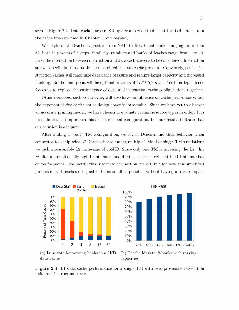
seen in Figure 2.4. Data cache lines are 8 4-byte words-wide (note that this is di↵erent from
the cache line size used in Chapter 3 and beyond).
We explore L1 Dcache capacities from 2KB to 64KB and banks ranging from 1 to
32, both in powers of 2 steps. Similarly, numbers and banks of Icaches range from 1 to 16.
First the interaction between instruction and data caches needs to be considered. Instruction
starvation will limit instruction issue and reduce data cache pressure. Conversely, perfect in-
struction caches will maximize data cache pressure and require larger capacity and increased
banking. Neither end-point will be optimal in terms of MRPS/mm
2. This interdependence
forces us to explore the entire space of data and instruction cache configurations together.
Other resources, such as the XUs, will also have an influence on cache performance, but
the exponential size of the entire design space is intractable. Since we have yet to discover
an accurate pruning model, we have chosen to evaluate certain resource types in order. It is
possible that this approach misses the optimal configuration, but our results indicate that
our solution is adequate.
After finding a “best” TM configuration, we revisit Dcaches and their behavior when
connected to a chip-wide L2 Dcache shared among multiple TMs. For single-TM simulations
we pick a reasonable L2 cache size of 256KB. Since only one TM is accessing the L2, this
results in unrealistically high L2 hit-rates, and diminishes the e↵ect that the L1 hit-rate has
on performance. We rectify this inaccuracy in section 2.2.2.3, but for now this simplified
processor, with caches designed to be as small as possible without having a severe impact
1 2 4 8 16 32
0%
10%
20%
30%
40%
50%
60%
70%
80%
90%
100%
Data Stall Bank Conflict
Issued
Perc
ent
of
Tota
l C
ycle
s
(a) Issue rate for varying banks in a 2KBdata cache
2KB 4KB 8KB 16KB 32KB 64KB
0%
10%
20%
30%
40%
50%
60%
70%
80%
90%
100%
Hit-Rate
(b) Dcache hit rate, 8-banks with varyingcapacities
Figure 2.4: L1 data cache performance for a single TM with over-provisioned executionunits and instruction cache.

18
on performance, provides a baseline for examining other resources, such as the execution
units.
2.2.2.2 Shared Execution Units
The next step is to consider sharing lightly used and area-expensive XUs for multiple
cores in a TM. The goal is area reduction without a commensurate decrease in performance.
Table 2.2 shows area estimates for each of our execution units. The integer multiply,
floating-point (FP) multiply, FP add/subtract, and FP inverse-square-root units dominate
the others in terms of area, thus sharing these units will have the greatest e↵ect on reducing
total TM area. In order to maintain a reasonably sized exploration space, these are the
only units considered as candidates for sharing. The other units are too small to have a
significant e↵ect on the performance-per-area metric.
We ran many thousands of simulations and varied the number of integer multiply, FP
multiply, FP add/subtract and FP inverse-square-root units from 1 to 32 in powers of 2
steps. Given N shared execution units, each unit is only connected to 32/N cores in order
to avoid complicated connection logic and area that would arise from full connectivity.
Scheduling conflicts to shared resources are resolved in a round-robin fashion.
Figure 2.5 shows that the number of XUs can be reduced without drastically lowering
the issue rate, and Table 2.3 shows the top four configurations that were found in this
phase of the design exploration. All of the top configurations use the cache setup found in
section 2.2.2.1: two instruction caches, each with 16 banks, and a 4KB L1 data cache with
8 banks and approximately 8% of cycles as data stalls for both our core-wide and chip-wide
simulations.
Data stall FU stall Issued
1 2 4 8 16
0%
20%
40%
60%
80%
100%
(a) FP Add/Sub(13% of Insts)
1 2 4 8 16
0%
20%
40%
60%
80%
100%
(b) FP Multiply(13% of Insts)
1 2 4 8 16
0%
20%
40%
60%
80%
100%
(c) FP 1/p
(0.4% of Insts)
1 2 4 8 16
0%
20%
40%
60%
80%
100%
(d) Int Multiply(0.3% of Insts)
Figure 2.5: E↵ect of shared execution units on issue rate shown as a percentage of totalcycles
19
Table 2.3: Optimal TM configurations in terms of MRPS/mm2.INT FP FP FP MRPS/ Area MRPS/MUL MUL ADD INV core (mm2) mm2
2 8 8 1 4.2 1.62 2.62 4 8 1 4.1 1.58 2.62 4 4 1 4.0 1.57 2.64 8 8 1 4.2 1.65 2.6
Area is drastically reduced from the original overprovisioned baseline, but performance
remains relatively unchanged. Table 2.4 compares raw compute and register resources for
our TM compared to a GTX285 SM. Our design space included experiments in which
additional thread contexts were added to the TMs, allowing context switching from a
stalled thread. These experiments resulted in 3-4% higher issue rate, but required much
greater register area for the additional thread contexts, so we do not include simultaneous
multithreading in future experiments.
2.2.2.3 Chip Level Organization
Given the TM configurations found in Section 2.2.2.2 that have the minimal set of
resources required to maintain high performance, we now explore the impact of tiling many
of these TMs on a chip. Our chip-wide design connects one or more TMs to an L2 Dcache,
with one or more L2 caches on the chip. Up to this point, all of our simulations have been
single-TM simulations which do not realistically model L1 to L2 memory tra�c. With many
TMs, each with an individual L1 cache and a shared L2 cache, bank conflicts will increase
and the hit-rate will decrease. This will require a bigger, more highly banked L2 cache.
Hit-rate in the L1 will also a↵ect the level of tra�c between the two levels of cache so we
Table 2.4: GTX285 SM vs. SPMD TM resource comparison. Area estimates are normal-ized to our estimated XU sizes from Table 2.2, not from actual GTX285 measurements.
GTX285 SPMDSM (8 cores) TM (32 cores)
Registers 16384 4096FPAdds 8 8FPMuls 8 8INTAdds 8 32INTMuls 8 2Spec op 2 1
Register Area (mm2) 2.43 0.61Compute Area (mm2) 0.43 0.26
20
must explore a new set of L1 and L2 cache configurations with a varying number of TMs
connected to the L2.
Once many TMs are connected to a single L2, relatively low L1 hit-rates of 80-86%
reported in some of the candidate configurations for a TM will likely put too much pressure
on the L2. Figure 2.6(b) shows the total percentage of cycles stalled due to L2 bank conflicts
for a range of L1 hit-rates. The 80-86% hit-rate, reported for some initial TM configurations,
results in roughly one third of cycles stalling due to L2 bank conflicts. Even small changes
in L1 hit-rate from 85% to 90% will have an e↵ect on reducing L1 to L2 bandwidth, due
to the high number of cores sharing an L2. We therefore explore a new set of data caches
that result in a higher L1 hit-rate.
We assume up to four L2 caches can fit on a chip with a reasonable interface to main
memory. Our target area is under 200mm2, so 80 TMs (2560 cores) will fit even at 2.5mm2
each. Section 2.2.2.2 shows a TM area of 1.6mm2 is possible, and the di↵erence provides
room for additional exploration. The 80 TMs are evenly spread over the multiple L2 caches.
With up to four L2 caches per chip, this results in 80, 40, 27, or 20 TMs per L2. Figure 2.6(c)
shows the percentage of cycles stalled due to L2 bank conflicts for a varying number of TMs
connected to each L2. Even with a 64KB L1 cache with 95% hit-rate, any more than 20
TMs per L2 results in >10% of cycles as L2 bank conflict stalls. We therefore chose to
arrange the proposed chip with four L2 caches serving 20 TMs each. Figure 2.2 shows how
individual TMs of 32 threads might be tiled in conjunction with their L2 caches.
128K
B
256K
B
512K
B
1M
B
2M
B
4M
B
0%
20%
40%
60%
80%
100%
L2 Hit-Rate
(a) Hit-rate for varying L2capacities with 20 TMsconnected to each L2
2KB 4KB 8KB 16KB 32KB 64KB
0%
20%
40%
60%
80%
100%
L1
Hit-Rate
L2 Bank
Conflicts
(b) Percentage of cycles notissued due to L2 bank con-flicts for varying L1 capaci-ties (and thus hit-rates) for20 TMs
20 27 40
0%
20%
40%
60%
80%
100%
Multi-Core L2 Bank Conflicts
Perc
ent of T
ota
l C
ycle
s
(c) L2 bank conflicts fora varying number of TMsconnected to each L2. EachTM has a 64KB L1 cachewith 95% hit-rate
Figure 2.6: L2 performance for 16 banks and TMs with the top configuration reported inTable 2.3.
21
The result of the design space exploration is a set of architectural configurations that
all fit in under 200mm2 and maintain high performance. A selection of these are shown in
Table 2.5 and are what we use to compare to the best known GPU ray tracer of the time in
Section 2.2.2.4. Note that the GTX285 has close to half the die area devoted to texturing
hardware, and none of the benchmarks reported in [4] or in our own studies use image-based
texturing. Thus it may not be fair to include texture hardware area in the MRPS/mm
2
metric. On the other hand, the results reported for the GTX285 do use the texture memory
to hold scene data for the ray tracer, so although it is not used for texturing, that memory
(which is a large portion of the hardware) is participating in the benchmarks.
Optimizing power is not a primary goal of the baseline TRaX design, and we address
power consumption by improving on the baseline architecture from Chapter 3 onward.
Still, to ensure we are within the realm of reason, we use energy and power estimates
from Cacti v6.5 and Synopsys DesignWare to calculate a rough estimate of our chip’s total
power consumption in these experiments. Given the top chip configuration reported in
Table 2.5, and activity factors reported by our simulator, we roughly estimate a chip power
consumption of 83 watts, which we believe is in the range of power densities for commercial
GPUs.
2.2.2.4 Baseline TRaX Results
To evaluate the results of our design space exploration we chose two candidate architec-
tures from the top performers: one with small area (147mm2) and the other with larger area
(175mm2) but higher raw performance (as seen in Table 2.5). We ran detailed simulations
of these configurations using the same three scenes as in [4] and using the same mix of
primary and secondary rays. Due to the widely di↵ering scenes and shading computations
Table 2.5: A selection of our top chip configurations and performance compared to anNVIDIA GTX285 and Copernicus. Copernicus area and performance are scaled to 65nmand 2.33 GHz to match the Xeon E5345, which was their starting point. Each of our SPMDThread Multiprocessors (TM) has 2 integer multiply, 8 FP multiply, 8 FP add, 1 FP invsqrtunit, and 2 16-banked Icaches.
L1 L1 L2 L2 L1 L2 Bandwidth (GB/s) Thread Area MRPS/
Size Banks Size Banks Hitrate Hitrate L1 L2 DRAM Issue (mm2) MRPS mm2
32KB 4 256KB 16 93% 75% 42 56 13 70% 147 322 2.232KB 4 512KB 16 93% 81% 43 57 10 71% 156 325 2.132KB 8 256KB 16 93% 75% 43 57 14 72% 159 330 2.132KB 8 512KB 16 93% 81% 43 57 10 72% 168 335 2.064KB 4 512KB 16 95% 79% 45 43 10 76% 175 341 1.9GTX285 (area is from 65nm GTX280 version for better comparison) 75% 576 111 0.2GTX285 SIMD core area only — no texture unit (area is estimated from die photo) 75% ~300 111 0.37Copernicus at 22nm, 4GHz, 115 Core2-style cores in 16 tiles 98% 240 43 0.18Copernicus at 22nm, 4GHz, with their envisioned 10x SW improvement 98% 240 430 1.8Copernicus with 10x SW improvement, scaled to 65nm, 2.33GHz 98% 961 250 0.26
22
used in [4] and [32], a direct comparison between both architectures is not feasible. We chose
to compare against [4] because it represents the best reported performance at the time for
a ray tracer running on a GPU, and their ray tracing application is more similar to ours.
We do, however, give a high level indication of the range of performance for our SPMD
architecture, GTX285 and Copernicus, in Table 2.5. In order to show a meaningful area
comparison, we used the area of a GTX280, which uses a 65nm process, and other than clock
frequency, is equivalent to the GTX285. Copernicus area is scaled up from 22nm to 65nm.
Assuming that their envisioned 240mm2 chip is 15.5mm on each side, a straightforward
scaling from 22nm to 65nm would be a factor of three increase on each side, but due to
certain process features not scaling linearly, we use a more realistic factor of two per side,
giving a total equivalent area of 961mm2 at 65nm. We then scaled the assumed 4GHz clock
frequency from Govindaraju et al. down to the actual 2.33GHz of the 65nm Clovertown core
on which their original scaling was based. The 10x scaling due to algorithmic improvements
in the Razor software used in the Copernicus system is theoretically envisioned [32].
The final results and comparisons to GTX285 are shown in Table 2.6. It is interesting to
note that although GTX285 and Copernicus take vastly di↵erent approaches to accelerating
ray-tracing, when scaled for performance/area they are quite similar. It is also interesting
to note that although our two candidate configurations perform di↵erently in terms of raw
performance, when scaled for MRPS/mm
2 they o↵er similar performance, especially for
secondary rays.
Table 2.6: Comparing our performance on two di↵erent core configurations to the GTX285for three benchmark scenes [4]. Primary ray tests consisted of 1 primary and 1 shadow rayper pixel. Di↵use ray tests consisted of 1 primary and 32 secondary global illumination raysper pixel.
Conference (282k triangles) Fairy (174k triangles) Sibenik (80k triangles)SPMD Ray SPMD SPMD SPMD SPMD SPMD SPMD
Type Issue Rate MRPS Issue Rate MRPS Issue Rate MRPS147mm2 Primary 74% 376 70% 369 76% 274
Di↵use 53% 286 57% 330 37% 107175mm2 Primary 77% 387 73% 421 79% 285
Di↵use 67% 355 70% 402 46% 131
SIMD Ray GTX GTX GTX GTX GTX GTXType SIMD e↵. MRPS SIMD e↵. MRPS SIMD e↵. MRPS
GTX285 Primary 74% 142 76% 75 77% 117Di↵use 46% 61 46% 41 49% 47
SPMD MRPS/mm2 ranges from 2.56 (Conference, primary rays) to 0.73 (Sibenik, di↵use rays) for both configsSIMD MRPS/mm2 ranges from 0.25 (Conference, primary rays) to 0.07 (Fairy, di↵use rays)SIMD (no texture area) MRPS/mm2 ranges from 0.47 (Conference, primary) to 0.14 (Fairy, di↵use)
23
When our raw speed is compared to the GTX285, our configurations are between 2.3x
and 5.6x faster for primary rays (average of 3.5x for the three scenes and two SPMD
configurations) and 2.3x to 9.8x faster for secondary rays (5.6x average). We can also see
that our thread issue rates do not change dramatically for primary vs. secondary rays,
especially for the larger of the two configurations. When scaled for MRPS/mm
2, our
configurations are between 8.0x and 19.3x faster for primary rays (12.4x average), and
8.9x to 32.3x faster for secondary rays (20x average). Even if we assume that the GTX285
texturing unit is not participating in the ray-tracing, and thus use a 2x smaller area estimate
for that processor, these speed-ups are still approximately 6x-10x on average.
We have developed a baseline custom ray-tracing architecture, with flexible programma-
bility and impressive performance, that we believe serves as an excellent platform for further
development. In the following chapters, we address the more important concerns of energy
consumption, while maintaining this baseline’s rays per second performance.
CHAPTER 3
RAY TRACING FROM A DATA
MOVEMENT PERSPECTIVE
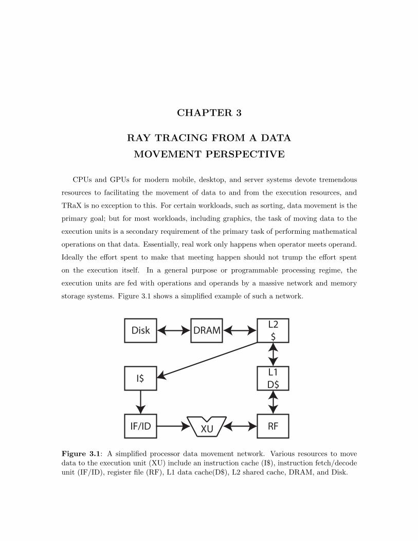
CPUs and GPUs for modern mobile, desktop, and server systems devote tremendous
resources to facilitating the movement of data to and from the execution resources, and
TRaX is no exception to this. For certain workloads, such as sorting, data movement is the
primary goal; but for most workloads, including graphics, the task of moving data to the
execution units is a secondary requirement of the primary task of performing mathematical
operations on that data. Essentially, real work only happens when operator meets operand.
Ideally the e↵ort spent to make that meeting happen should not trump the e↵ort spent
on the execution itself. In a general purpose or programmable processing regime, the
execution units are fed with operations and operands by a massive network and memory
storage systems. Figure 3.1 shows a simplified example of such a network.
RFIF/ID
I$ L1D$
L2$
XU
DRAMDisk
Figure 3.1: A simplified processor data movement network. Various resources to movedata to the execution unit (XU) include an instruction cache (I$), instruction fetch/decodeunit (IF/ID), register file (RF), L1 data cache(D$), L2 shared cache, DRAM, and Disk.
25
For each atom of work (instruction), some or all of the following memory systems must
be activated:
• Instruction Fetch - the instruction is fetched from an instruction cache to the
decoder/execution unit. In a general purpose processor, an instruction is typically
a single mathematical operation, such as comparing or multiplying two numbers.
• Register File - operands for the instruction are fetched from the register file and a
result may be sent back to the register file.
• Main Memory Hierarchy - the register file and instruction cache are backed by the
main memory hierarchy. In the case of overflowing, instructions, operands, or results
are fetched from/sent to the main memory hierarchy, activating potentially all of the
following systems:
– Cache Hierarchy - if the working set of data is too large for the register file,
data is is transferred to and from the cache hierarchy, consisting of one or more
levels of on-chip memory. If the data required is not found in the first level, the
next level is searched, and so on. Typically each consecutive level of cache is
larger, slower, and more energy consumptive than the previous. The goal of this
hierarchy is to keep data as close to the register file and instruction fetch units
as possible.
– DRAM - if the data is not found in the cache hierarchy, it must be transferred
from o↵-chip DRAM, which is much larger, slower, and more energy consumptive
than the caches.
– Disk - in the event the data is not even contained in DRAM, the much slower
disk or network storage must be accessed. This is not common in real-time
rendering systems, and we will not focus on this interface, although it is a major
concern in o✏ine rendering [26].
The interfaces between these memory components can only support a certain maximum
data transfer rate (bandwidth). If any particular memory interface cannot provide data
as fast as the execution units require it, that interface becomes a bottleneck preventing
execution from proceeding any faster. If this happens, although execution units may be
available to perform work, they have no data to perform work on. Designing a high
performance compute system involves finding the right balance of execution and data

26
movement resources within the constraints of the chip, limited not only by die area, but
also power consumption [23, 87]. Table 3.1 shows the simulated area, energy, and latency
costs for the execution units and various data movement resources in a basic many-core
TRaX system. We can see that the balance of resources is tipped heavily in favor of
data movement, and this is not unique to TRaX. This balance can be tuned with both
hardware and software techniques. Since di↵erent applications can have widely varying
data movement requirements, we can take heavy advantage of specialization if the desired
application domain is known ahead of time.
An application specific integrated circuit (ASIC) takes specialization to the extreme and
can achieve vast improvements in energy e�ciency over a general purpose programmable
processor [24, 58, 39]. Instead of performing a sequence of generic single instructions at a
time, which combined makes up a more complex programmable function, an ASIC performs
exactly one specific function. These functions are typically much more complex than the
computation performed by a single general purpose instruction, and the circuitry for the
function is hard-wired on the chip. This fixed-function circuitry removes some of the data
movement overheads discussed above. Specifically, instructions need not be fetched, and
operands and intermediate results flow directly from one execution unit to the next, avoiding
expensive round trips to the register file and/or data caches. These overheads can be up
to 20⇥ more energy consumptive than the execution units themselves [36]. The downside
to an ASIC is the lack of programmability. If the desired computation changes, an ASIC
cannot adapt.
Less extreme specialization techniques can have many of the same energy saving benefits
as an ASIC but without sacrificing as much programmability. If the application can take
advantage of SIMD parallelism, the cost of fetching an instruction for a specific operation is
amortized over multiple sets of parallel data operands. An N-way SIMD processor fetches
up to N⇥ fewer instructions to perform the same work as a scalar processor working
on parallel data. Alternatively, very large instruction word (VLIW) architectures encode
multiple operations into a single instruction. This makes the instructions larger, but a
Table 3.1: Resource cost breakdown for a 2560-thread TRaX processor.Die Area (mm2) Avg. Activation Energy (nJ) Avg. Latency (ns)
Execution Units 36.7 0.004 1.35Register Files 73.5 0.008 1
Instruction Caches 20.9 0.013 1Data Caches 45.5 0.174 1.06
DRAM n/a 20 - 70 20 - 200
27
single instruction fetched can perform a complex computation kernel that is the equivalent
of many simpler single instructions. This requires the compiler to be able to identify these
kernels in a programmable workload. Adding VLIW and SIMD execution to an otherwise
general purpose processor, Hameed et al. report a tenfold reduction in the instruction fetch
energy consumption when operating on certain workloads [36].
Even within a general purpose domain, many applications exhibit common microkernels
of computation, such as multiply-accumulate, in which the product of two numbers must
be added to an accumulator. This is a common operation in many algorithms, including
computer graphics. Similar to an ASIC, the two operations can be fused into a pipeline
and activated with a single instruction, and unlike VLIW, the instruction word size does
not need to increase. Although the kernel is much smaller than a typical ASIC pipeline,
it provides many of the same benefits while retaining programmability. The benefit gained
from this type of operation fusion depends on how frequently the kernel is used. Hameed
et al. report an extra 1.1⇥-to-1.9⇥ energy reduction in the instruction fetch and register
file energy, on top of existing VLIW and SIMD enhancements [36].
Prebaked fused operations in a general purpose architecture such as multiply-add are
necessarily very simple in order to be broadly applicable. An application may have unique
microkernels that a chip designer could not anticipate. CoGene [80] is a compiler system
that automatically detects the data movement needs of kernels within a program, and
dynamically generates “fused” operations by rerouting data through a flexible interconnect,
given the resources available on the chip. Such a system can provide greater ASIC-like
benefits than the simplest assumed micro kernels like multiply-add, yet avoid becoming
overly specific to remain applicable to a wide range of applications.
As previously mentioned, if the application domain is known, further opportunities can
be exploited. Particularly, graphics workloads consist of large amounts of 3D vector math,
such as vector addition or dot products. Table 3.2 summarizes the potential energy savings
for fusing various common 3D vector operations in a TRaX system. If vector operands
were encoded with a single base register address, the instruction size would not increase. In
Section 3.2, we explore even further specialized fused operations specifically for ray traced
graphics.
The data cache hierarchy exists to relieve pressure on the main DRAM. The goal is to
keep portions of main memory data as close to the execution units as possible to reduce
the cost of data movement. If successful, the portions kept in the cache at any given time
are the portions that will need frequent reuse during and around that time period. From a
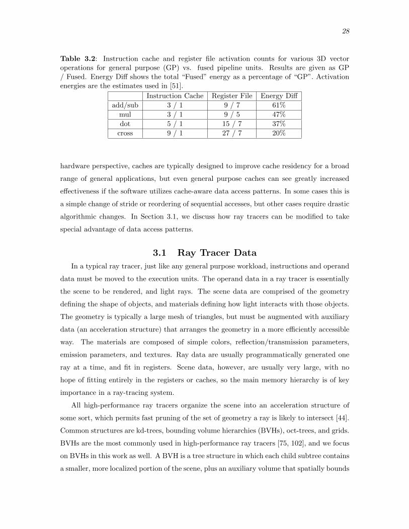
28
Table 3.2: Instruction cache and register file activation counts for various 3D vectoroperations for general purpose (GP) vs. fused pipeline units. Results are given as GP/ Fused. Energy Di↵ shows the total “Fused” energy as a percentage of “GP”. Activationenergies are the estimates used in [51].
Instruction Cache Register File Energy Di↵add/sub 3 / 1 9 / 7 61%mul 3 / 1 9 / 5 47%dot 5 / 1 15 / 7 37%cross 9 / 1 27 / 7 20%
hardware perspective, caches are typically designed to improve cache residency for a broad
range of general applications, but even general purpose caches can see greatly increased
e↵ectiveness if the software utilizes cache-aware data access patterns. In some cases this is
a simple change of stride or reordering of sequential accesses, but other cases require drastic
algorithmic changes. In Section 3.1, we discuss how ray tracers can be modified to take
special advantage of data access patterns.
3.1 Ray Tracer DataIn a typical ray tracer, just like any general purpose workload, instructions and operand
data must be moved to the execution units. The operand data in a ray tracer is essentially
the scene to be rendered, and light rays. The scene data are comprised of the geometry
defining the shape of objects, and materials defining how light interacts with those objects.
The geometry is typically a large mesh of triangles, but must be augmented with auxiliary
data (an acceleration structure) that arranges the geometry in a more e�ciently accessible
way. The materials are composed of simple colors, reflection/transmission parameters,
emission parameters, and textures. Ray data are usually programmatically generated one
ray at a time, and fit in registers. Scene data, however, are usually very large, with no
hope of fitting entirely in the registers or caches, so the main memory hierarchy is of key
importance in a ray-tracing system.
All high-performance ray tracers organize the scene into an acceleration structure of
some sort, which permits fast pruning of the set of geometry a ray is likely to intersect [44].
Common structures are kd-trees, bounding volume hierarchies (BVHs), oct-trees, and grids.
BVHs are the most commonly used in high-performance ray tracers [75, 102], and we focus
on BVHs in this work as well. A BVH is a tree structure in which each child subtree contains
a smaller, more localized portion of the scene, plus an auxiliary volume that spatially bounds
29
that portion of the scene. Determining the geometry a ray may intersect involves traversing
this tree based on whether or not the ray intersects the bounding volume of any given node.
The order that nodes are traversed, and thus loaded from memory, is very unpredictable,
particularly when global illumination e↵ects generate random and incoherent rays. This
unpredictable memory access pattern makes it very challenging for the cache hierarchy
to keep a working set of data near the execution units for very long. This problem is
exacerbated when parallel execution threads traverse multiple rays simultaneously using a
shared cache, since individual rays can take drastically di↵erent paths through the BVH.
Finding cache-friendly access patterns in BVH traversal is not a trivial task, and requires
significant algorithmic changes as opposed to, for example, simply reordering the access
order of a loop. Recent work has explored a variety of ways to increase data access e�ciency
in ray-tracing. These approaches typically involve grouping rays together and processing
more than one at a time. Usually these groups are either spatially coherent rays, i.e.,
rays with a common origin and similar direction, or more directly, structurally coherent
rays, i.e., rays known to access the same portions of the acceleration structure. Software
approaches involve gathering rays into coherent packets to better match the SIMD execution
model [9, 12, 34, 73]. These systems also tend to increase cache hit rates because the ray
packets operate on similar regions of interest. Packet techniques can have limited utility
with highly incoherent rays, since packets must be broken apart if rays within them do not
follow the same path through the BVH.
More directly related to this work, specific approaches to more e↵ective memory band-
width utilization can involve cache-conscious data organization [77, 20, 78, 57], and ray
reordering [95, 13, 68, 61]. Some researchers employ image-space rather than data-space
partitioning for rays [45, 14, 15]. Stream-based approaches to ray generation and processing
have also been explored both in a ray-tracing context [33, 82, 97, 2, 67] and a volume-
rendering context [22]. Although technical details are limited, at least two commercial
hardware approaches to ray-tracing appear to use some sort of ray sorting and/or classifi-
cation [59, 90]. PowerVR [59] enqueues rays at each node in the BVH, deferring processing
until a bundle of them are available, and using a sophisticated scheduler to decide which
bundle to process next.
3.1.1 Treelets
We use a form of ray reordering based on recent work [67, 2], in which rays are specifically
grouped together based on their location in the acceleration structure, allowing certain
guarantees about data access coherence. The BVH tree is partitioned into sub-groups
30
called treelets, sized to fit comfortably in either the L1 or L2 data cache. Each node in
the BVH belongs to exactly one treelet, and treelet identification tags are stored along
with the node ID. During traversal, when a ray crosses a treelet boundary, it is sent to a
corresponding ray bu↵er, where its computation is deferred until a processor is assigned to
that bu↵er. In this scheme, a processor will work for a prolonged period of time only on rays
that traverse a single treelet. This allows that subset of BVH data (the treelet) to remain in
the processor’s cache for a long time and drastically increase cache hit rates. This technique
requires many rays to be in flight at once in order to fill the treelet ray bu↵ers, as opposed
to the typical single ray or small ray packet per core model. The state of each ray must
be stored in global memory and passed along to other processors as needed. Ideally, this
auxiliary ray state storage should not increase o↵-chip bandwidth consumption drastically,
since reducing DRAM bandwidth is the end goal.
Both Navratil et al. [67] and Aila et al.[2] store treelet ray bu↵ers in main memory.
While this does generate extra DRAM tra�c in the form of rays, it reduces geometry tra�c
by a greater amount. Navratil et al. report up to 32⇥ reduction in DRAM tra�c for
primary rays, and 60⇥ for shadow rays, while Aila et al. extend the work to massively
parallel GPU architectures and report a tenfold reduction for di�cult scenes rendered with
global illumination.
3.2 Streaming Treelet Ray Tracing Architecture(STRaTA)
We expand on treelet techniques with hardware support for ray bu↵ers and also take
advantage of opportunities in the data access patterns imposed by the algorithmic changes
for processing treelets. In contrast to previous work, we store the ray state in a bu↵er
on-chip, therefore storing or retrieving rays does not a↵ect the consumed DRAM bandwidth,
however, the added on-chip data movement costs must still be carefully considered. We
combine this with additional hardware specialization for reducing the instruction fetch and
register file data movement using reconfigurable macro instruction pipelines, which are
dynamically configured under program control (Section 7.1.2). These pipelines consist of
execution units (XUs), multiplexers (MUXs), and latches that are shared by multiple thread
processors. We construct two special purpose pipelines: one for bounding volume hierarchy
box intersection and the other for triangle intersection. The essential benefit of this tactic
is to replace a large number of conventional instructions with a single large fused box or
triangle intersection instruction, similar to the techniques discussed earlier in this Chapter
and in Table 3.2. The energy e�ciency of these pipelines is similar to an ASIC design

31
except for the relatively small energy overhead incurred by the MUXs and slightly longer
wire lengths [58, 39, 80]. However, unlike ASICs, our pipelines are flexible, since they are
configured under program control.
We will use TRaX as a starting point, since it has demonstrated impressive preliminary
performance and is supported by powerful simulation and compiler toolchains [38]. These
tools make the architecture, ISA, and API amenable to modifications as needed.
3.2.1 Ray Stream Bu↵ers
We adapt Aila’s approach by partitioning a special purpose ray stream memory that
replaces some or all of the L2 data cache. This avoids auxiliary tra�c by never saving ray
state o↵-chip, at the cost of a lower total number of rays in flight, which are limited by the
size of the ray stream partition. The TRaX architecture uses very simple direct-mapped
caches, which save area and power over more complex associative caches. We assign treelets
to be exactly the size of an L1 cache, and the BVH builder arranges the treelets into cache-
aligned contiguous address spaces. Since the L1 only contains treelet data, this guarantees
that while a TM is working on a specific treelet, each line in the TM’s L1 cache will incur
at most one miss, and will be transferred to the L1 only once.
We also modify Aila’s algorithm to di↵erentiate triangle data from BVH data, and
assign each to a separate type of treelet (see Figure 3.2). Note that triangle treelets are
not technically a “tree,” but simply a collection of triangles in nearby leaf nodes. This
ensures that any TM working on a leaf or triangle treelet is doing nothing but triangle
intersections, allowing us to configure a specialized pipeline for triangle intersection (see
Section 7.1.2). Similarly, when working on a nonleaf BVH treelet, the TM is computing
only ray-box intersections, utilizing a box intersection pipeline.
The ray stream memory holds the ray bu↵ers for every treelet. Any given ray bu↵er can
potentially hold anywhere from zero rays up to the maximum number that fit in the stream
memory, leaving no room for any of the other bu↵ers. The capacity of each ray bu↵er is
thus limited by the number of rays in every other bu↵er. Although the simulator models
these dynamically-sized ray bu↵ers as a simple collection data structure, we envision a
hardware model in which they are implemented using a hardware managed linked-list state
machine with a pointer to the head of each bu↵er stored in the SRAM. Link pointers for
the nodes and a free list could be stored within the SRAM as well. This would occupy a
small portion of the potential ray memory: not enough to drastically a↵ect the total number
of rays in flight, since it requires eight percent or less of the total capacity for our tested
configurations. The energy cost of an address lookup for the head of the desired ray bu↵er,
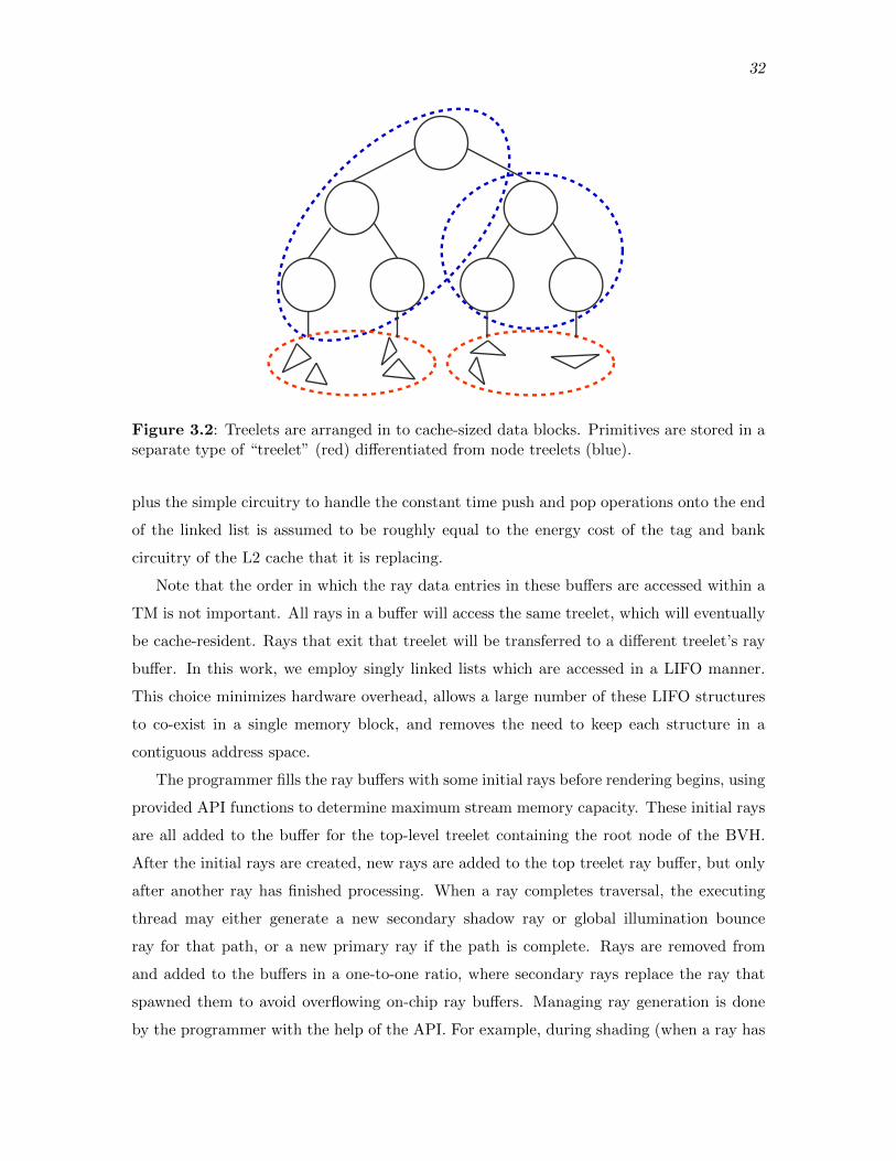
32
Figure 3.2: Treelets are arranged in to cache-sized data blocks. Primitives are stored in aseparate type of “treelet” (red) di↵erentiated from node treelets (blue).
plus the simple circuitry to handle the constant time push and pop operations onto the end
of the linked list is assumed to be roughly equal to the energy cost of the tag and bank
circuitry of the L2 cache that it is replacing.
Note that the order in which the ray data entries in these bu↵ers are accessed within a
TM is not important. All rays in a bu↵er will access the same treelet, which will eventually
be cache-resident. Rays that exit that treelet will be transferred to a di↵erent treelet’s ray
bu↵er. In this work, we employ singly linked lists which are accessed in a LIFO manner.
This choice minimizes hardware overhead, allows a large number of these LIFO structures
to co-exist in a single memory block, and removes the need to keep each structure in a
contiguous address space.
The programmer fills the ray bu↵ers with some initial rays before rendering begins, using
provided API functions to determine maximum stream memory capacity. These initial rays
are all added to the bu↵er for the top-level treelet containing the root node of the BVH.
After the initial rays are created, new rays are added to the top treelet ray bu↵er, but only
after another ray has finished processing. When a ray completes traversal, the executing
thread may either generate a new secondary shadow ray or global illumination bounce
ray for that path, or a new primary ray if the path is complete. Rays are removed from
and added to the bu↵ers in a one-to-one ratio, where secondary rays replace the ray that
spawned them to avoid overflowing on-chip ray bu↵ers. Managing ray generation is done
by the programmer with the help of the API. For example, during shading (when a ray has
33
completed traversal/intersection), if another ray must be generated as part of the shader,
the programmer simply adds that ray with the same pixel ID and updated state (such as
ray type) to the root treelet ray bu↵er, instead of immediately invoking a BVH traversal
routine.
Each ray requires 48 bytes comprised of: ray origin and direction (24 bytes total), ray
state (current BVH node index, closest hit, traversal state, ray type, etc. totaling 20 bytes),
and a traversal stack (4 bytes, see Section 3.2.2).
3.2.2 Traversal Stack
E�cient BVH traversal attempts to minimize the number of nodes traversed by finding
the closest hit point as early as possible. If a hit point is known and it lies closer than
the intersection with a BVH node, then the traversal can terminate early by ignoring that
branch of the tree. To increase the chances of terminating early, most ray tracers traverse
the closer BVH child first. Since it is nondeterministic which child was visited first, typically
a traversal stack is used to keep track of nodes that need to be visited at each level. One can
avoid a stack altogether by adding parent pointers to the BVH, and using a deterministic
traversal order (such as always left first, then right), this, however, eliminates the possibility
of traversing the closer child first and results in less e�cient traversal.
Streaming approaches, such as the one used in this work, typically require additional
memory space to store ray state. Rays are passed around from core to core via memory
bu↵ers. In our case, the more rays present in a bu↵er, the longer a TM can operate on
that treelet, increasing the energy savings by not accessing o↵-chip memory during that
computation. Storing the entire traversal stack with every ray has a very large memory
cost, and would reduce the total number of rays in flight significantly. There have been
a number of recent techniques to reduce or eliminate the storage size of a traversal stack,
at the cost of extra work during traversal or extra data associated with the BVH, such as
parent pointers [91, 53, 37].
We use a traversal technique in which parent pointers are included with the BVH, so
full node IDs are not required for each branch decision. We do, however, need to keep track
of which direction (left child or right child) was taken first at each node. To reduce the
memory cost of keeping this information, we store the direction as a single bit on a stack,
and thus a 32-entry stack fits in one integer. Furthermore, there is no need for a stack
pointer, as it is implied that the least significant bit (LSB) is the top of the stack. Stack
operations are simple bitwise integer manipulations: shift left one bit to push, shift right
one bit to pop. In this scheme, after a push, either 1 is added to the stack (setting the LSB
34
to 1, corresponding to left), or it is left alone (leaving the LSB as 0, corresponding to right).
After visiting a node’s subtree, we examine the top of the stack. If the direction indicated
on the top of the stack is equal to which side the visited child was on, then we traverse the
other child if necessary; otherwise we are done with both children and pop the stack and
continue moving up the tree.
3.2.3 Reconfigurable Pipelines
One of the characteristics of ray-tracing is that computation can be partitioned into
distinct phases: traversal, intersection, and shading. The traversal and intersection phases
have a small set of specific computations that dominate time and energy consumption. If the
available XUs in a TM could be connected so that data could flow directly through a series
of XUs without fetching new instructions for each operation, a great deal of instruction
fetch and register file access energy could be saved. We propose repurposing the XUs by
temporarily reconfiguring them into a combined ray-triangle or ray-box intersection test
unit using a series of latches and MUXs when the computation phase can make e↵ective use
of that functionality. The overhead for this reconfigurability (i.e. time, energy and area)
is fairly low, as the MUXs and latches are small compared to the size of the floating-point
XUs, which themselves occupy a small portion of the circuit area of a TM [58, 39, 81, 80].
Consider a hardware pipeline test for a ray intersection with an axis-aligned box. The
inputs are four 3D vectors representing the two corners of the bounding box, the ray origin,
and ray direction (12 floats total). Although the box is stored as two points, it is treated
as three pairs of planes – one for each dimension in 3D [91, 104]. The interval of the ray’s
intersection distance between the near and far plane for each pair is computed, and if there
is overlap between all three intervals, the ray hits the box, otherwise it misses. The bulk of
this computation consists of six floating-point multiplies and six floating-point subtracts,
followed by several comparisons to determine if the intervals overlap. Figure 3.3 shows a
data-flow representation of ray-box intersection, which we use to determine how to connect
the available XUs into a macroinstruction pipeline.
The baseline TRaX processor has eight floating point multiply, and eight floating point
add/subtract units shared within a TM, which was shown to be an optimal configuration in
terms of area and utilization for simple path tracing [52]. Our ray-box intersection pipeline
uses six multipliers and six add/subtract units, leaving two of each for general purpose use.
The comparison units are simple enough that adding extra ones as needed for the pipeline
to each TM has a negligible e↵ect on die area. The multiply and add/subtract units have
a latency of two cycles in 65nm at 1GHz, and the comparisons have a latency of one cycle.

35
corner1
FPSUB
3
ray origin
3
FPSUB
3
ray direction
FPMUL
3
FPMUL
3
corner2
3
3 3
FPMIN
3
FPMAX
3 3 3
FPMAX
3
FPMIN
<
1
>
1
3
1
&&
1 1
0
1
result
Figure 3.3: Data-flow representation of ray-box intersection. The red boxes at the topare the inputs (3D vectors), and the red box at the bottom is the output. Edge weightsindicate operand width.
The box-test unit can thus be fully pipelined with an initiation interval of one and a latency
of eight cycles.
Ray-triangle intersection is typically determined based on barycentric coordinates [60],
and is considerably more complex than ray-box intersection. We remapped the computation
as a data-flow graph, and investigated several potential pipeline configurations. Because an
early stage of the computation requires a high-latency divide (16 cycles), all of the options
have prohibitively long initiation intervals, and result in poor utilization of execution units
and low performance. An alternative technique uses Plucker coordinates to determine
hit/miss information [88], and requires the divide at the end of the computation, but only
if an intersection occurs. If a ray intersects a triangle, we perform the divide as a separate
operation outside of the pipeline (Figure 3.4). Of the many possible ray-triangle intersection
pipelines, we select one with a minimal resource requirement of four multipliers and two
adders, which results in an initiation interval of 18, a latency of 31 cycles, and an issue
width of two.

36
nu
FPMUL FPMUL
np
FPSUB
nv
FPMULFPMUL
pu
FPSUB
pv
FPSUB
e0u
FPMUL
e0v
FPMUL
e1u
FPMUL
e1v
FPMUL
org.u org.vorg.w
FPADD
dir.u
FPMUL
dir.v
FPMUL
dir.w
FPADD
FPADDFPADD
FPMUL FPMUL
FPSUB
FPSUB FPSUB
FPSUB
same sign?
FPSUB
FPSUB
result
Figure 3.4: Data-flow representation of ray-triangle intersection using Plucker coordi-nates [88]. The red boxes at the top are the inputs, and the red box at the bottom is theoutput. All edges represent scalar operands.
The final stage shades the ray without reconfiguring the TM pipeline. In our test scenes,
Lambertian shading is a small portion of the total computation, and threads performing
shading can take advantage of the leftover general purpose XUs without experiencing severe
starvation. Alternatively, if shading were more computationally intensive or if the data
footprint of the materials were large, the rays could be sent to a separate bu↵er or be
processed by a pipeline configured for shading.
The programmer invokes and configures these phase-specific pipelines with simple com-
piler intrinsics provided in the API. Once a TM is configured into a specific pipeline,
all of the TPs within operate in the same mode until reconfigured. Since the pipelines
have many inputs, the programmer is also responsible for loading the input data (a ray
and a triangle/box) into special input registers via the API and compiler intrinsics. This
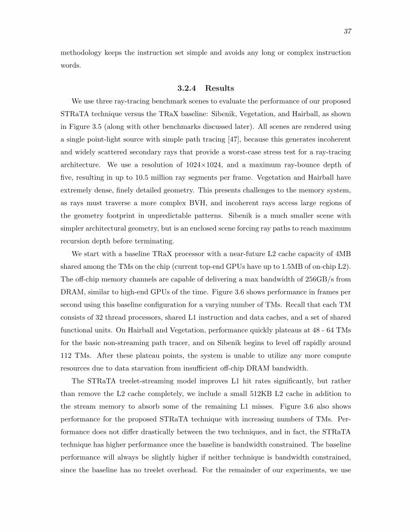
37
methodology keeps the instruction set simple and avoids any long or complex instruction
words.
3.2.4 Results
We use three ray-tracing benchmark scenes to evaluate the performance of our proposed
STRaTA technique versus the TRaX baseline: Sibenik, Vegetation, and Hairball, as shown
in Figure 3.5 (along with other benchmarks discussed later). All scenes are rendered using
a single point-light source with simple path tracing [47], because this generates incoherent
and widely scattered secondary rays that provide a worst-case stress test for a ray-tracing
architecture. We use a resolution of 1024⇥1024, and a maximum ray-bounce depth of
five, resulting in up to 10.5 million ray segments per frame. Vegetation and Hairball have
extremely dense, finely detailed geometry. This presents challenges to the memory system,
as rays must traverse a more complex BVH, and incoherent rays access large regions of
the geometry footprint in unpredictable patterns. Sibenik is a much smaller scene with
simpler architectural geometry, but is an enclosed scene forcing ray paths to reach maximum
recursion depth before terminating.
We start with a baseline TRaX processor with a near-future L2 cache capacity of 4MB
shared among the TMs on the chip (current top-end GPUs have up to 1.5MB of on-chip L2).
The o↵-chip memory channels are capable of delivering a max bandwidth of 256GB/s from
DRAM, similar to high-end GPUs of the time. Figure 3.6 shows performance in frames per
second using this baseline configuration for a varying number of TMs. Recall that each TM
consists of 32 thread processors, shared L1 instruction and data caches, and a set of shared
functional units. On Hairball and Vegetation, performance quickly plateaus at 48 - 64 TMs
for the basic non-streaming path tracer, and on Sibenik begins to level o↵ rapidly around
112 TMs. After these plateau points, the system is unable to utilize any more compute
resources due to data starvation from insu�cient o↵-chip DRAM bandwidth.
The STRaTA treelet-streaming model improves L1 hit rates significantly, but rather
than remove the L2 cache completely, we include a small 512KB L2 cache in addition to
the stream memory to absorb some of the remaining L1 misses. Figure 3.6 also shows
performance for the proposed STRaTA technique with increasing numbers of TMs. Per-
formance does not di↵er drastically between the two techniques, and in fact, the STRaTA
technique has higher performance once the baseline is bandwidth constrained. The baseline
performance will always be slightly higher if neither technique is bandwidth constrained,
since the baseline has no treelet overhead. For the remainder of our experiments, we use
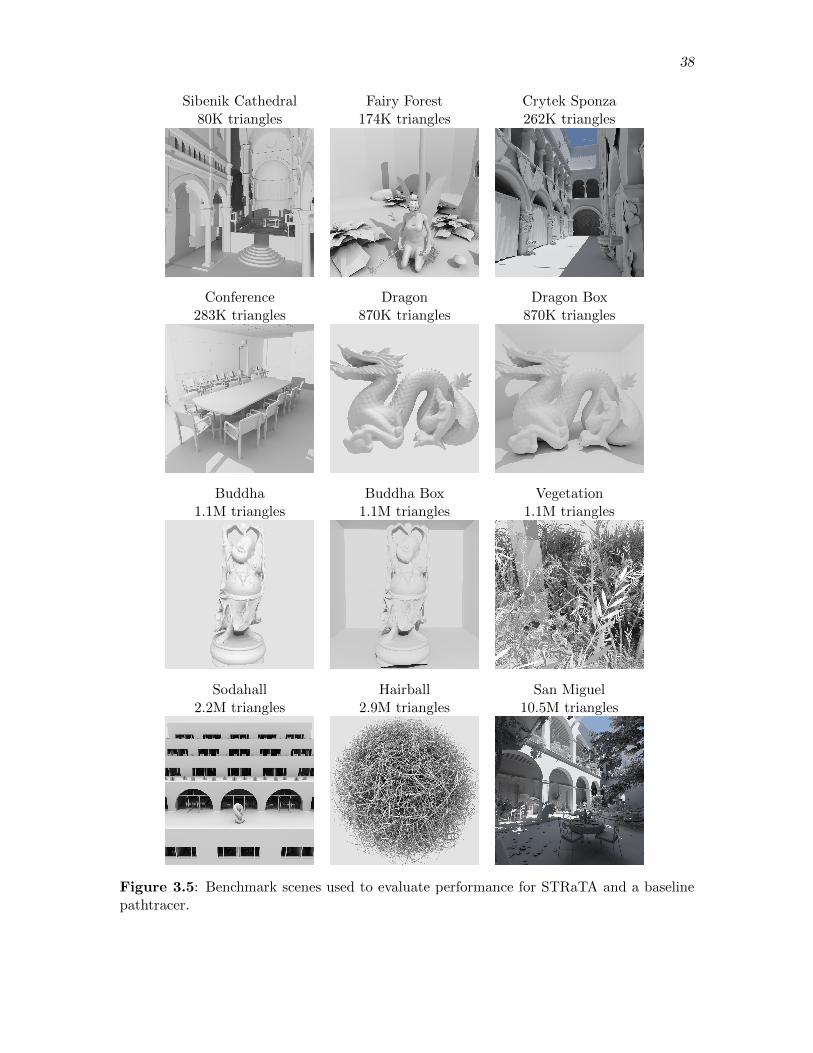
38
Sibenik Cathedral80K triangles
Fairy Forest174K triangles
Crytek Sponza262K triangles
Conference283K triangles
Dragon870K triangles
Dragon Box870K triangles
Buddha1.1M triangles
Buddha Box1.1M triangles
Vegetation1.1M triangles
Sodahall2.2M triangles
Hairball2.9M triangles
San Miguel10.5M triangles
Figure 3.5: Benchmark scenes used to evaluate performance for STRaTA and a baselinepathtracer.
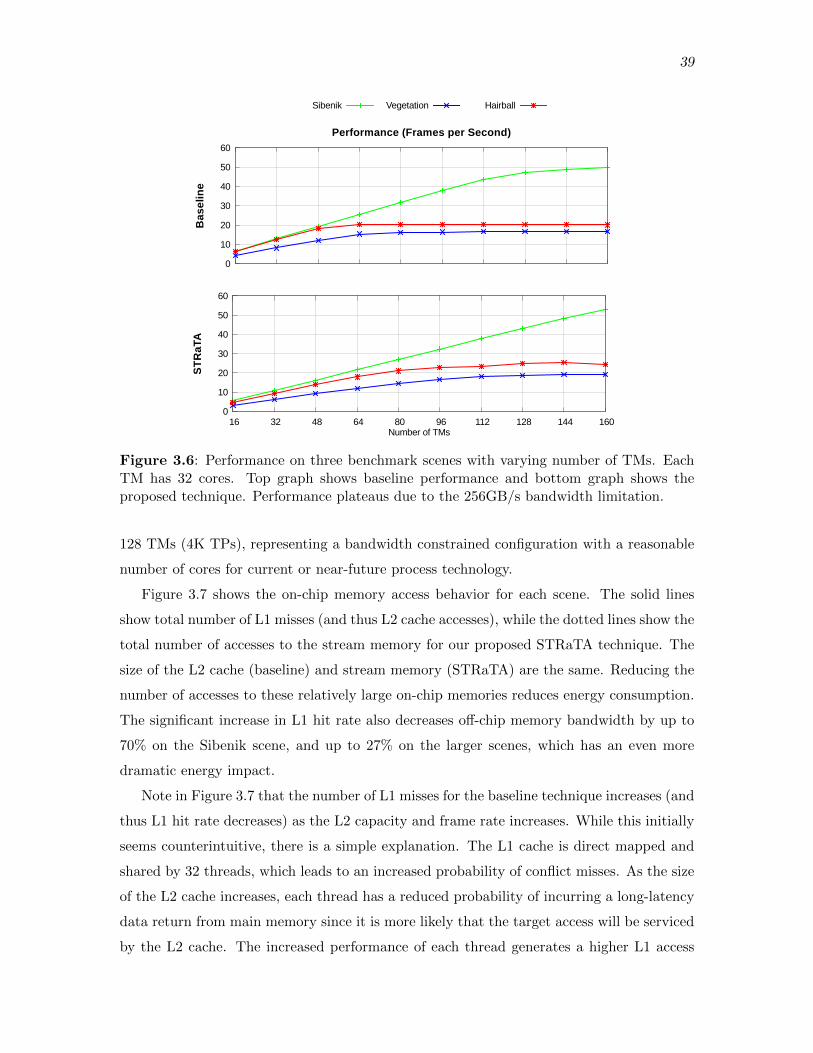
39
0
10
20
30
40
50
60
Bas
elin
e
Performance (Frames per Second)
Sibenik Vegetation Hairball
0
10
20
30
40
50
60
16 32 48 64 80 96 112 128 144 160
STR
aTA
Number of TMs
Figure 3.6: Performance on three benchmark scenes with varying number of TMs. EachTM has 32 cores. Top graph shows baseline performance and bottom graph shows theproposed technique. Performance plateaus due to the 256GB/s bandwidth limitation.
128 TMs (4K TPs), representing a bandwidth constrained configuration with a reasonable
number of cores for current or near-future process technology.
Figure 3.7 shows the on-chip memory access behavior for each scene. The solid lines
show total number of L1 misses (and thus L2 cache accesses), while the dotted lines show the
total number of accesses to the stream memory for our proposed STRaTA technique. The
size of the L2 cache (baseline) and stream memory (STRaTA) are the same. Reducing the
number of accesses to these relatively large on-chip memories reduces energy consumption.
The significant increase in L1 hit rate also decreases o↵-chip memory bandwidth by up to
70% on the Sibenik scene, and up to 27% on the larger scenes, which has an even more
dramatic energy impact.
Note in Figure 3.7 that the number of L1 misses for the baseline technique increases (and
thus L1 hit rate decreases) as the L2 capacity and frame rate increases. While this initially
seems counterintuitive, there is a simple explanation. The L1 cache is direct mapped and
shared by 32 threads, which leads to an increased probability of conflict misses. As the size
of the L2 cache increases, each thread has a reduced probability of incurring a long-latency
data return from main memory since it is more likely that the target access will be serviced
by the L2 cache. The increased performance of each thread generates a higher L1 access
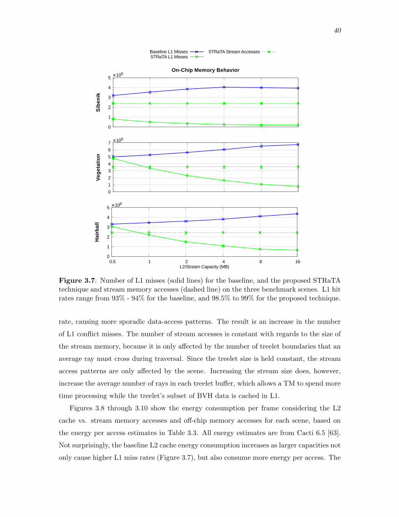
40
0
1
2
3
4
5
Sib
enik
On-Chip Memory Behavior ×108
Baseline L1 MissesSTRaTA L1 Misses
STRaTA Stream Accesses
0
1
2
3
4
5
6
7
Vege
tatio
n
×108
0
1
2
3
4
5
0.5 1 2 4 8 16
Hai
rbal
l
L2/Stream Capacity (MB)
×108
Figure 3.7: Number of L1 misses (solid lines) for the baseline, and the proposed STRaTAtechnique and stream memory accesses (dashed line) on the three benchmark scenes. L1 hitrates range from 93% - 94% for the baseline, and 98.5% to 99% for the proposed technique.
rate, causing more sporadic data-access patterns. The result is an increase in the number
of L1 conflict misses. The number of stream accesses is constant with regards to the size of
the stream memory, because it is only a↵ected by the number of treelet boundaries that an
average ray must cross during traversal. Since the treelet size is held constant, the stream
access patterns are only a↵ected by the scene. Increasing the stream size does, however,
increase the average number of rays in each treelet bu↵er, which allows a TM to spend more
time processing while the treelet’s subset of BVH data is cached in L1.
Figures 3.8 through 3.10 show the energy consumption per frame considering the L2
cache vs. stream memory accesses and o↵-chip memory accesses for each scene, based on
the energy per access estimates in Table 3.3. All energy estimates are from Cacti 6.5 [63].
Not surprisingly, the baseline L2 cache energy consumption increases as larger capacities not
only cause higher L1 miss rates (Figure 3.7), but also consume more energy per access. The

41
0
0.1
0.2
0.3
0.4
0.5
0.6
0.7
L2 E
nerg
y
ener
gy/fr
ame
(Jou
les)
Sibenik
Baseline STRaTA
0 0.2 0.4 0.6 0.8
1 1.2 1.4 1.6 1.8
0.5 1 2 4 8 16
Mai
n M
emor
y E
nerg
y
ener
gy/fr
ame
(Jou
les)
L2/Stream Capacity (MB)
Figure 3.8: E↵ect of L2 cache size (Baseline) and stream memory size (STRaTA) onmemory system energy for the Sibenik scene.
0
0.2
0.4
0.6
0.8
1
1.2
L2 E
nerg
y
ener
gy/fr
ame
(Jou
les)
Vegetation
Baseline STRaTA
0 0.5
1 1.5
2 2.5
3 3.5
4
0.5 1 2 4 8 16
Mai
n M
emor
y E
nerg
y
ener
gy/fr
ame
(Jou
les)
L2/Stream Capacity (MB)
Figure 3.9: E↵ect of L2 cache size (Baseline) and stream memory size (STRaTA) onmemory system energy for the Vegetation scene.
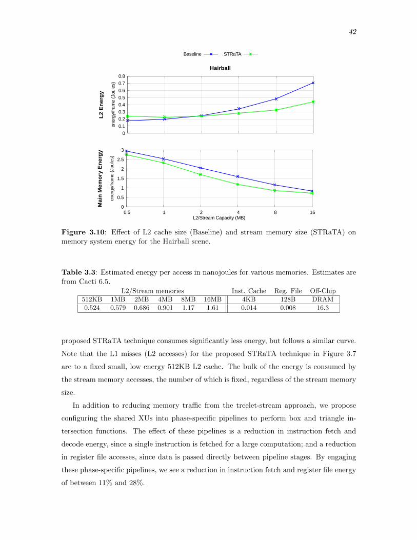
42
0 0.1 0.2 0.3 0.4 0.5 0.6 0.7 0.8
L2 E
nerg
y
ener
gy/fr
ame
(Jou
les)
Hairball
Baseline STRaTA
0
0.5
1
1.5
2
2.5
3
0.5 1 2 4 8 16
Mai
n M
emor
y E
nerg
y
ener
gy/fr
ame
(Jou
les)
L2/Stream Capacity (MB)
Figure 3.10: E↵ect of L2 cache size (Baseline) and stream memory size (STRaTA) onmemory system energy for the Hairball scene.
Table 3.3: Estimated energy per access in nanojoules for various memories. Estimates arefrom Cacti 6.5.
L2/Stream memories Inst. Cache Reg. File O↵-Chip512KB 1MB 2MB 4MB 8MB 16MB 4KB 128B DRAM0.524 0.579 0.686 0.901 1.17 1.61 0.014 0.008 16.3
proposed STRaTA technique consumes significantly less energy, but follows a similar curve.
Note that the L1 misses (L2 accesses) for the proposed STRaTA technique in Figure 3.7
are to a fixed small, low energy 512KB L2 cache. The bulk of the energy is consumed by
the stream memory accesses, the number of which is fixed, regardless of the stream memory
size.
In addition to reducing memory tra�c from the treelet-stream approach, we propose
configuring the shared XUs into phase-specific pipelines to perform box and triangle in-
tersection functions. The e↵ect of these pipelines is a reduction in instruction fetch and
decode energy, since a single instruction is fetched for a large computation; and a reduction
in register file accesses, since data is passed directly between pipeline stages. By engaging
these phase-specific pipelines, we see a reduction in instruction fetch and register file energy
of between 11% and 28%.

43
The total energy used per frame for a path tracer in this TRaX-style architecture is
a function of the size of the L2 cache or stream memory, and whether the phase-specific
pipelines are used. If we combine the two enhancements, we see a total reduction in energy
of the memory system (on- and o↵-chip memory and register file) and the instruction fetch
of up to 38%. These reductions in energy come from relatively simple modifications to the
basic parallel architecture with negligible overhead. They also have almost no impact on
the frames per second performance, and actually increase the performance slightly in some
cases. Although the functional unit energy has not changed, the significant reductions in
energy used in the various memory systems, combined with low hardware overhead, implies
that these techniques would be welcome additions to any hardware architecture targeting
ray-tracing.
These results are promising, but turn out to be somewhat optimistic. We will see in
Chapter 4 how the simple model for memory used in the TRaX simulator is masking some
important behavior with respect to o↵-chip DRAM. We will rectify this simplification in
Chapter 4, and show how to exploit more detailed knowledge of DRAM circuits in Chapter 5.
With a more accurate DRAMmodel, the total energy savings is slightly less, which reinforces
the importance of accurate memory simulations.

CHAPTER 4
DRAM
DRAM can be the primary consumer of energy in a graphics system, as well as the
main performance bottleneck. Due to the massive size of geometry and materials in typical
scenes, accessing DRAM is unavoidable. In Chapter 3, we discussed various techniques
to reduce the number and frequency of DRAM accesses, primarily by increasing cache hit
rates. While it is certainly true that reducing the number of DRAM accesses can be an
e↵ective means of reducing energy consumption and easing the bottleneck, a detailed look at
the structure of DRAM circuits reveals that changing the data access patterns is an equally
or more e↵ective means of reducing energy costs. This is true even in cases where the raw
data consumption increases over the baseline system. Furthermore, utilizing the maximum
bandwidth capabilities of a DRAM system is essentially impossible for typical unmanaged
access patterns. The more carefully we control DRAM access patterns, the more e↵ectively
we can utilize its capabilities.
The simulations performed in Section 3.2, and in many other works of architecture
exploration, use a simplistic model for accessing DRAM. In the TRaX simulator, a DRAM
access was assumed to have a fixed average latency and energy consumption. This can
drastically misrepresent both time and energy consumption. The maximum bandwidth
was naıvely limited by only allowing a certain number of accesses per cycle, ignoring
access patterns and queueing. This would allow for any access pattern to achieve the
maximum capable bandwidth, and would not bu↵er requests to accommodate bursts and
calm periods. A simple DRAM model such as this may be su�cient for general-purpose
or non-memory-bound application simulation, but if we are truly concerned with memory
activity and wish to take advantage of DRAM characteristics, we must model the subtleties
of its behavior. Modeling DRAM correctly is nontrivial, and can have very important
implications on results.
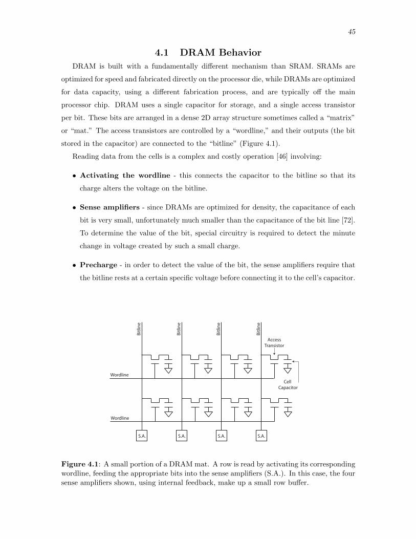
45
4.1 DRAM BehaviorDRAM is built with a fundamentally di↵erent mechanism than SRAM. SRAMs are
optimized for speed and fabricated directly on the processor die, while DRAMs are optimized
for data capacity, using a di↵erent fabrication process, and are typically o↵ the main
processor chip. DRAM uses a single capacitor for storage, and a single access transistor
per bit. These bits are arranged in a dense 2D array structure sometimes called a “matrix”
or “mat.” The access transistors are controlled by a “wordline,” and their outputs (the bit
stored in the capacitor) are connected to the “bitline” (Figure 4.1).
Reading data from the cells is a complex and costly operation [46] involving:
• Activating the wordline - this connects the capacitor to the bitline so that its
charge alters the voltage on the bitline.
• Sense amplifiers - since DRAMs are optimized for density, the capacitance of each
bit is very small, unfortunately much smaller than the capacitance of the bit line [72].
To determine the value of the bit, special circuitry is required to detect the minute
change in voltage created by such a small charge.
• Precharge - in order to detect the value of the bit, the sense amplifiers require that
the bitline rests at a certain specific voltage before connecting it to the cell’s capacitor.
S.A.
Wordline
S.A. S.A. S.A.
Wordline
Bitli
ne
Bitli
ne
Bitli
ne
Bitli
ne
AccessTransistor
Cell Capacitor
Figure 4.1: A small portion of a DRAM mat. A row is read by activating its correspondingwordline, feeding the appropriate bits into the sense amplifiers (S.A.). In this case, the foursense amplifiers shown, using internal feedback, make up a small row bu↵er.
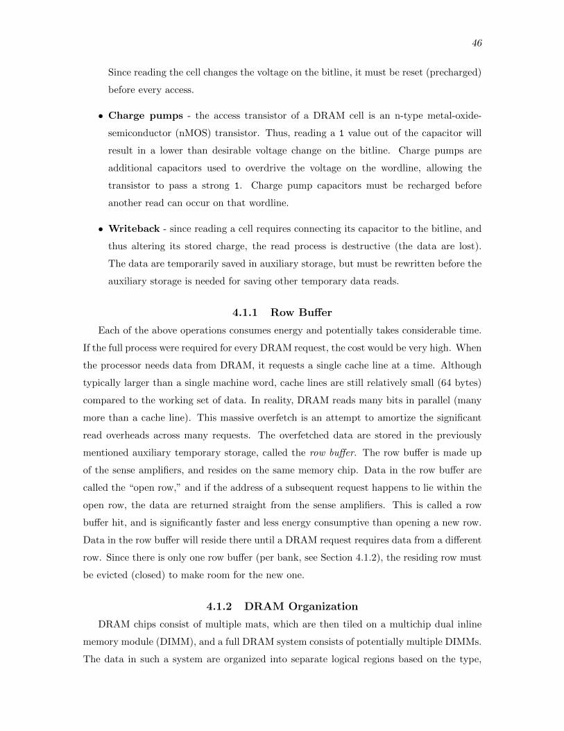
46
Since reading the cell changes the voltage on the bitline, it must be reset (precharged)
before every access.
• Charge pumps - the access transistor of a DRAM cell is an n-type metal-oxide-
semiconductor (nMOS) transistor. Thus, reading a 1 value out of the capacitor will
result in a lower than desirable voltage change on the bitline. Charge pumps are
additional capacitors used to overdrive the voltage on the wordline, allowing the
transistor to pass a strong 1. Charge pump capacitors must be recharged before
another read can occur on that wordline.
• Writeback - since reading a cell requires connecting its capacitor to the bitline, and
thus altering its stored charge, the read process is destructive (the data are lost).
The data are temporarily saved in auxiliary storage, but must be rewritten before the
auxiliary storage is needed for saving other temporary data reads.
4.1.1 Row Bu↵er
Each of the above operations consumes energy and potentially takes considerable time.
If the full process were required for every DRAM request, the cost would be very high. When
the processor needs data from DRAM, it requests a single cache line at a time. Although
typically larger than a single machine word, cache lines are still relatively small (64 bytes)
compared to the working set of data. In reality, DRAM reads many bits in parallel (many
more than a cache line). This massive overfetch is an attempt to amortize the significant
read overheads across many requests. The overfetched data are stored in the previously
mentioned auxiliary temporary storage, called the row bu↵er. The row bu↵er is made up
of the sense amplifiers, and resides on the same memory chip. Data in the row bu↵er are
called the “open row,” and if the address of a subsequent request happens to lie within the
open row, the data are returned straight from the sense amplifiers. This is called a row
bu↵er hit, and is significantly faster and less energy consumptive than opening a new row.
Data in the row bu↵er will reside there until a DRAM request requires data from a di↵erent
row. Since there is only one row bu↵er (per bank, see Section 4.1.2), the residing row must
be evicted (closed) to make room for the new one.
4.1.2 DRAM Organization
DRAM chips consist of multiple mats, which are then tiled on a multichip dual inline
memory module (DIMM), and a full DRAM system consists of potentially multiple DIMMs.
The data in such a system are organized into separate logical regions based on the type,
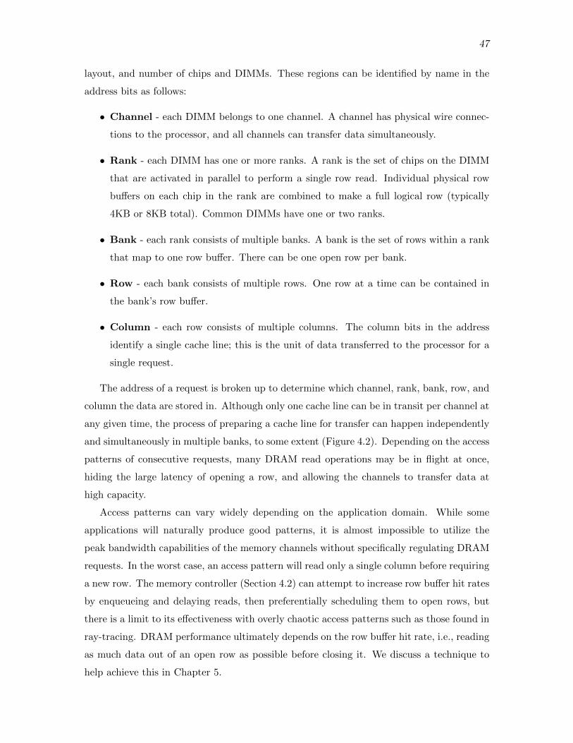
47
layout, and number of chips and DIMMs. These regions can be identified by name in the
address bits as follows:
• Channel - each DIMM belongs to one channel. A channel has physical wire connec-
tions to the processor, and all channels can transfer data simultaneously.
• Rank - each DIMM has one or more ranks. A rank is the set of chips on the DIMM
that are activated in parallel to perform a single row read. Individual physical row
bu↵ers on each chip in the rank are combined to make a full logical row (typically
4KB or 8KB total). Common DIMMs have one or two ranks.
• Bank - each rank consists of multiple banks. A bank is the set of rows within a rank
that map to one row bu↵er. There can be one open row per bank.
• Row - each bank consists of multiple rows. One row at a time can be contained in
the bank’s row bu↵er.
• Column - each row consists of multiple columns. The column bits in the address
identify a single cache line; this is the unit of data transferred to the processor for a
single request.
The address of a request is broken up to determine which channel, rank, bank, row, and
column the data are stored in. Although only one cache line can be in transit per channel at
any given time, the process of preparing a cache line for transfer can happen independently
and simultaneously in multiple banks, to some extent (Figure 4.2). Depending on the access
patterns of consecutive requests, many DRAM read operations may be in flight at once,
hiding the large latency of opening a row, and allowing the channels to transfer data at
high capacity.
Access patterns can vary widely depending on the application domain. While some
applications will naturally produce good patterns, it is almost impossible to utilize the
peak bandwidth capabilities of the memory channels without specifically regulating DRAM
requests. In the worst case, an access pattern will read only a single column before requiring
a new row. The memory controller (Section 4.2) can attempt to increase row bu↵er hit rates
by enqueueing and delaying reads, then preferentially scheduling them to open rows, but
there is a limit to its e↵ectiveness with overly chaotic access patterns such as those found in
ray-tracing. DRAM performance ultimately depends on the row bu↵er hit rate, i.e., reading
as much data out of an open row as possible before closing it. We discuss a technique to
help achieve this in Chapter 5.

48
(a) Same Row
Row 0
Row 1
Col 0 Col 1 Col 0 Col 1
Row 0
Row 1
Channel 0 Channel 1
Bank 0
Bank 1
Load A
Load B
Open Row Column Access Transfer
Writeback
tRAS
A B
Column Access Transfer
tCCD
tRCD
tCAS
time
(b) Separate Channels
Row 0
Row 1
Col 0 Col 1 Col 0 Col 1
Row 0
Row 1
Channel 0 Channel 1
Bank 0
Bank 1
Load A
Load B
Open Row Column Access Transfer
WritebackA B
Open Row Column Access Transfer
Writeback
(c) Di↵erent Banks Within Same Channel
Row 0
Row 1
Col 0 Col 1 Col 0 Col 1
Row 0
Row 1
Channel 0 Channel 1
Bank 0
Bank 1
Load A
Load B
Open Row Column Access Transfer
Writeback
tRRD
A
B
Open Row Column Access Transfer
Writeback
(d) Di↵erent Rows Within Same Bank
Row 0
Row 1
Col 0 Col 1 Col 0 Col 1
Row 0
Row 1
Channel 0 Channel 1
Bank 0
Bank 1
Load A
Load B
Open Row Column Access Transfer
Writeback
tRC
Precharge
Open Row ...
...
A
B
Figure 4.2: Simple DRAM access timing examples showing the processing of two simul-taneous read requests (load A and B).
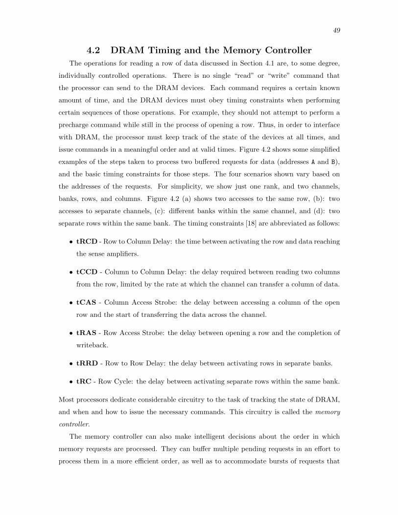
49
4.2 DRAM Timing and the Memory ControllerThe operations for reading a row of data discussed in Section 4.1 are, to some degree,
individually controlled operations. There is no single “read” or “write” command that
the processor can send to the DRAM devices. Each command requires a certain known
amount of time, and the DRAM devices must obey timing constraints when performing
certain sequences of those operations. For example, they should not attempt to perform a
precharge command while still in the process of opening a row. Thus, in order to interface
with DRAM, the processor must keep track of the state of the devices at all times, and
issue commands in a meaningful order and at valid times. Figure 4.2 shows some simplified
examples of the steps taken to process two bu↵ered requests for data (addresses A and B),
and the basic timing constraints for those steps. The four scenarios shown vary based on
the addresses of the requests. For simplicity, we show just one rank, and two channels,
banks, rows, and columns. Figure 4.2 (a) shows two accesses to the same row, (b): two
accesses to separate channels, (c): di↵erent banks within the same channel, and (d): two
separate rows within the same bank. The timing constraints [18] are abbreviated as follows:
• tRCD - Row to Column Delay: the time between activating the row and data reaching
the sense amplifiers.
• tCCD - Column to Column Delay: the delay required between reading two columns
from the row, limited by the rate at which the channel can transfer a column of data.
• tCAS - Column Access Strobe: the delay between accessing a column of the open
row and the start of transferring the data across the channel.
• tRAS - Row Access Strobe: the delay between opening a row and the completion of
writeback.
• tRRD - Row to Row Delay: the delay between activating rows in separate banks.
• tRC - Row Cycle: the delay between activating separate rows within the same bank.
Most processors dedicate considerable circuitry to the task of tracking the state of DRAM,
and when and how to issue the necessary commands. This circuitry is called the memory
controller.
The memory controller can also make intelligent decisions about the order in which
memory requests are processed. They can bu↵er multiple pending requests in an e↵ort to
process them in a more e�cient order, as well as to accommodate bursts of requests that

50
arrive faster than serviceable. For example, if several requests reside in the bu↵er, some of
them in one row, and some of them in another, the memory controller may service all of
the requests to one row first, regardless of the order in which they arrived.
4.3 Accurate DRAM ModelingTRaX’s naıve DRAM assumptions would not capture any of the important behavior
discussed above, and may cause egregious errors in the results. The mechanisms and
constraints of DRAM can clearly have an e↵ect on performance. If we are to truly study
the e↵ect of streaming data techniques on arguably the most important component of the
memory hierarchy, we must model the cycle-to-cycle memory controller and DRAM chip
state, and expose the following phenomena in a simulator:
• Opening/closing rows, row bu↵er hits vs. misses - These can result in drastic
di↵erences in energy and delay.
• Scheduling - Reads can be serviced out of order, which results in opportunities for
increasing row hits. This also a↵ects on-chip cache performance.
• Write drain mode - Draining the write queue disables reads for a long period of
time, introducing hiccups in DRAM access timing.
• Refresh - Memory cells must be rewritten periodically or they lose data. This disables
large sections of memory for a long period of time, introducing hiccups and consuming
a large amount of energy.
• Separate memory clock - A memory controller can make decisions in-between or
slower than GPU/CPU cycles.
• Address mapping policy - The way in which addresses are mapped to chan-
nels/banks/rows has a direct impact on how e�ciently the data is accessed.
• Background energy - DRAM energy is not only a function of the number and
pattern of accesses, but also of running time.
USIMM (Utah Simulated Memory Module) is a DRAM simulator with sophisticated
modeling of timing and energy characteristics for the entire DRAM system [18], and has
been used by a number of simulation systems as an accurate memory model [62, 66]. In
this work, we incorporate USIMM into the TRaX simulator, and adapt it to operate with
on-the-fly DRAM requests as they are generated, as opposed to operating on trace files.

51
The result is a fully cycle accurate GPU system simulator with USIMM dynamically serving
at the top of the memory hierarchy. We use this to further explore the problem of data
movement in ray-tracing with a focus on the very important DRAM interface in Chapter 5.

CHAPTER 5
STREAMING THROUGH DRAM
A fair amount of recent work, including our own (see Chapter 3), aims to reduce o↵-chip
data consumption, since DRAM can be the main performance bottleneck in a ray tracer and
is a very large energy consumer (Figure 1.1, Table 3.1). Raw data consumption, however,
does not tell the full story, since the internal structure of DRAM yields highly variable
energy and latency characteristics depending on access patterns. A benchmark with a
higher number of total accesses but a friendlier access pattern may outperform another
benchmark that consumes less raw data. Essentially, DRAM e�ciency comes down to row
bu↵er hit rate: the higher the better.
As discussed in Chapter 4, the memory controller can attempt to increase the row bu↵er
hit rate given whatever accesses the application generates, but with limited e↵ectiveness.
If the application consciously orders its data accesses to address the nature of DRAM,
the memory controller can be vastly more successful in finding row bu↵er hits. STRaTA
(Section 3.2) reorders memory accesses with the goal of increasing cache hit rates, but this
also reveals a fortuitous opportunity when considering the complexities of DRAM.
To understand the key di↵erence in DRAM access patterns between the baseline path
tracer and STRaTA, we must examine the algorithmic source of the accesses. The baseline’s
memory access pattern is determined by the nature of the BVH traversal algorithm. Since
no special care is taken to govern memory access patterns, the result is chaotic accesses
when global illumination inevitably generates many incoherent rays. Accesses that miss in
the L1 and L2 are thus both temporally and spatially incoherent, generating continuous
moderate pressure on all channels, banks, and rows in DRAM.
STRaTA remaps the ray-tracing algorithm to specifically target coherent L1 accesses.
While a TM is operating on a certain treelet, all accesses will hit in the L1, except for the
first to any given cache line. Ideally a TM will operate on the treelet for a prolonged period
of time, generating no L2 or DRAM accesses. The accesses that do make it past the L1 occur
right after a TM has switched to a new treelet; all threads within a TM will immediately
53
begin reading cache lines for the new treelet, missing in the L1, and generating a very large
burst of L2/DRAM accesses. While the small L2 cache in STRaTA may absorb some of
this burst, the remainder that makes it to DRAM will have the same bursty structure, but
will be no larger than the size of a treelet.
The optimal size of STRaTA’s treelets was determined experimentally to be as close to
the capacity of the L1 cache as possible [50], which is 16KB. We can thus guarantee that
the burst to load a treelet from DRAM is no larger than 16KB, however, depending on the
BVH builder and treelet assignment algorithm, a treelet’s data may be scattered arbitrarily
throughout memory. The only requirements of STRaTA’s (and most ray tracers’) BVH
layout is that siblings reside next to each other in memory; we can rearrange the data at
will so long as this restriction is met. We thus modify the BVH builder so that all nodes
belonging to one treelet are stored in a consecutive address block. The result is that the
large DRAM burst to load a treelet maps directly to just two rows (Figure 5.1).
Since the burst takes place over a short period of time, the memory controller’s read
queues will fill with an abundance of same-row requests, making it trivial to schedule reads
for row bu↵er hits. The memory controller’s address mapping policy places consecutive
cache lines (columns) in the same row, and strides consecutive rows across the memory
channels (Figure 5.1). This allows for the two rows making up a treelet to be transferred
simultaneously from two separate channels (Figure 4.2(b)). We call this new modified
version “STRaTA+.”
Row 0
Row 2 Row 4 Row 6
…
Row 1
Row 3 Row 5 Row 7
…
Channel 0 Channel 1
DRAM
Figure 5.1: Treelets are arranged in contiguous data blocks targeted as a multiple of theDRAM row size. In this example treelets are constructed to be the size of two DRAM rows.Primitives are stored in a separate type of “treelet” di↵erentiated from node treelets, andsubject to the same DRAM row sizes.
54
5.1 AnalysisWe start with the baseline TRaX system discussed in Section 3.2.4, based on previous
performance/area explorations [52] (see Section 2.2), with 128 TMs, which results in
4K total thread processors. To model near-future GPU DRAM capabilities, we configure
USIMM for both the baseline and STRaTA+ to use GDDR5 with eight 64-bit channels,
running at 2GHz (8GHz e↵ective), for a total of 512GB/s maximum bandwidth. The GPU
core configurations use a 1GHz clock rate.
We update the experiments performed in Section 3.2 with the improved DRAM simulator
and with the new row-friendly data ordering for STRaTA+. We also include many more
benchmark scenes (Figure 3.5). Since the mix of geometric complexity and data footprints
can have a large impact on a ray tracer’s performance, it is imperative to test a wide range
of scenes [3]. The scenes used include: architectural models (Sibenik, Crytek, Conference,
Sodahall, San Miguel), scanned models (Buddha, Dragon), and nature/game models (Fairy,
Vegetation, Hairball). The laser scan models are unlikely to be used alone in empty space
in a real situation such as a movie or game, so we also include versions of them enclosed in
a box, allowing rays to bounce around the environment.
Because STRaTA stores rays in on-chip bu↵ers with finite capacity, rays must be gen-
erated and consumed in a one-to-one ratio (Section 3.2.1). This limits our test renderer to
shading with nonbranching ray paths. To support more advanced shaders, the programmer
could add more information to the per-ray state to determine the remaining rays yet to
be generated. When one shading ray finishes, a new ray could be generated with updated
state for the associated shading point. Increasing the data footprint of rays will reduce the
number of them that fit in the stream memory, but our results indicate that the number
of rays in flight could decrease by a fair amount without being detrimental to the system.
Another option is to allow the on-chip ray bu↵ers to overflow to main memory when full
(for example Aila et al. store rays in main memory [2]), but this would require carefully
regulating when and where the data is uploaded to DRAM in order to maintain the theme
of intelligent access patterns. Since we do not focus on shading in this work, we leave this
as a future exercise, discussed in Section 7.1.
5.2 ResultsTable 5.1 shows a breakdown of various DRAM characteristics on each scene, as well
as total running time in ms/frame, for the baseline and STRaTA+ techniques. Note
that although STRaTA+ increases L1 hit rates, the lack of a large L2 cache can result in a
greater number of total DRAM accesses and thus increased bandwidth consumption on some
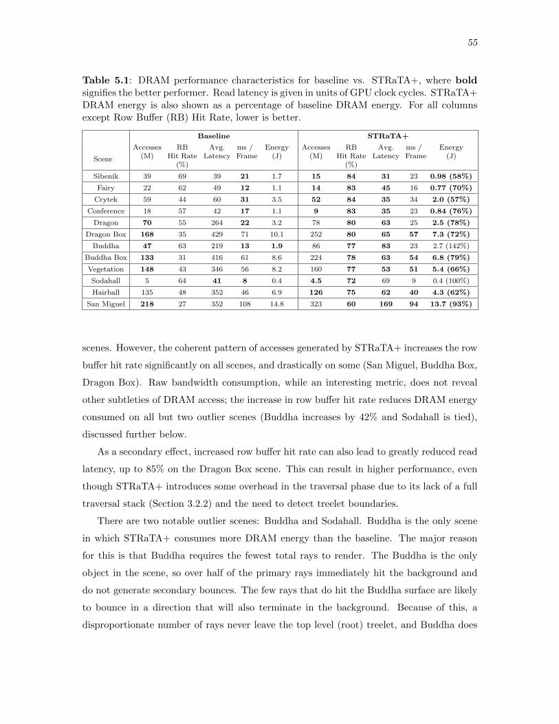
55
Table 5.1: DRAM performance characteristics for baseline vs. STRaTA+, where boldsignifies the better performer. Read latency is given in units of GPU clock cycles. STRaTA+DRAM energy is also shown as a percentage of baseline DRAM energy. For all columnsexcept Row Bu↵er (RB) Hit Rate, lower is better.
Baseline STRaTA+
Scene
Accesses(M)
RBHit Rate
(%)
Avg.Latency
ms /Frame
Energy(J)
Accesses(M)
RBHit Rate
(%)
Avg.Latency
ms /Frame
Energy(J)
Sibenik 39 69 39 21 1.7 15 84 31 23 0.98 (58%)
Fairy 22 62 49 12 1.1 14 83 45 16 0.77 (70%)
Crytek 59 44 60 31 3.5 52 84 35 34 2.0 (57%)
Conference 18 57 42 17 1.1 9 83 35 23 0.84 (76%)
Dragon 70 55 264 22 3.2 78 80 63 25 2.5 (78%)
Dragon Box 168 35 429 71 10.1 252 80 65 57 7.3 (72%)
Buddha 47 63 219 13 1.9 86 77 83 23 2.7 (142%)
Buddha Box 133 31 416 61 8.6 224 78 63 54 6.8 (79%)
Vegetation 148 43 346 56 8.2 160 77 53 51 5.4 (66%)
Sodahall 5 64 41 8 0.4 4.5 72 69 9 0.4 (100%)
Hairball 135 48 352 46 6.9 126 75 62 40 4.3 (62%)
San Miguel 218 27 352 108 14.8 323 60 169 94 13.7 (93%)
scenes. However, the coherent pattern of accesses generated by STRaTA+ increases the row
bu↵er hit rate significantly on all scenes, and drastically on some (San Miguel, Buddha Box,
Dragon Box). Raw bandwidth consumption, while an interesting metric, does not reveal
other subtleties of DRAM access; the increase in row bu↵er hit rate reduces DRAM energy
consumed on all but two outlier scenes (Buddha increases by 42% and Sodahall is tied),
discussed further below.
As a secondary e↵ect, increased row bu↵er hit rate can also lead to greatly reduced read
latency, up to 85% on the Dragon Box scene. This can result in higher performance, even
though STRaTA+ introduces some overhead in the traversal phase due to its lack of a full
traversal stack (Section 3.2.2) and the need to detect treelet boundaries.
There are two notable outlier scenes: Buddha and Sodahall. Buddha is the only scene
in which STRaTA+ consumes more DRAM energy than the baseline. The major reason
for this is that Buddha requires the fewest total rays to render. The Buddha is the only
object in the scene, so over half of the primary rays immediately hit the background and
do not generate secondary bounces. The few rays that do hit the Buddha surface are likely
to bounce in a direction that will also terminate in the background. Because of this, a
disproportionate number of rays never leave the top level (root) treelet, and Buddha does
56
not reach a critical mass of rays required for our ray bu↵ers to function e↵ectively. Hence,
we also consider a more realistic scene by placing Buddha in a box.
When a TM switches to a treelet ray bu↵er, if there are not enough rays to keep all of its
threads busy, many of the compute resources sit idle, e↵ectively reducing parallelism. Even
though STRaTA+ increases row bu↵er hit rates on Buddha, the increase in DRAM energy is
partly background energy caused by the nearly doubled running time while threads sit idle.
We note that DRAM energy is not only a function of the number and pattern of accesses, but
it also has a dependency on the total running time (e.g. ms/frame in Table 5.1), mostly
due to the need for continuous refreshing of the DRAM data even when no read/write
activity occurs, and because we use an open row memory controller policy [83] that keeps
rows open (consuming energy) for as long as possible in order to improve row bu↵er hit
rate.
Also note that the baseline has a relatively high row bu↵er hit rate on Buddha, so
STRaTA+ is unable to make as large of a di↵erence. The Dragon scene is similar to
Buddha, but does not exhibit this problem. The baseline takes almost twice as long to
render Dragon than Buddha, since Dragon fills a larger portion of the frame. This closes
the gap in background energy between the two techniques. Dragon also results in more
total rays, and has a smaller data footprint with fewer total treelets, and thus more rays on
average in each bu↵er.
The other interesting outlier is Sodahall. Even though it has a large data footprint (2.2M
triangles), it generates by far the fewest DRAM accesses. Most of the geometry is not visible
from any one viewing angle, since it is separated into many individual rooms. The BVH
does its job well, so only a small percentage of the total data is ever accessed. The pressure
on DRAM is so low that background energy is the dominant factor for both STRaTA+ and
the baseline. The viewpoint shown (Figure 3.5) has similar results to viewpoints inside the
building.
In addition to reducing energy consumption, STRaTA+ can also increase performance
scalability with the number of cores. Figure 5.2 shows performance for STRaTA+ with
increasing numbers of TMs (dotted lines), compared to the baseline (solid lines) for a subset
of benchmark scenes, and includes accurate DRAM modeling, unlike Figure 3.6. Since
DRAM is the bottleneck in both cases, this data becomes much more revealing. Memory
becomes a bottleneck much more quickly for the baseline than for STRaTA+, which is able
to utilize more cores to achieve significantly higher performance. In fact, we were unable to
find the plateau point for STRaTA+ for some scenes due to limited simulation time.
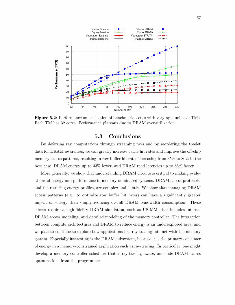
57
0
10
20
30
40
50
60
70
80
90
100
32 64 96 128 160 192 224 256 288 320
Pe
rfo
rma
nc
e (
FP
S)
Number of TMs
Sibenik BaselineCrytek Baseline
Vegetation BaselineHairball Baseline
Sibenik STRaTACrytek STRaTA
Vegetation STRaTAHairball STRaTA
Figure 5.2: Performance on a selection of benchmark scenes with varying number of TMs.Each TM has 32 cores. Performance plateaus due to DRAM over-utilization.
5.3 ConclusionsBy deferring ray computations through streaming rays and by reordering the treelet
data for DRAM awareness, we can greatly increase cache hit rates and improve the o↵-chip
memory access patterns, resulting in row bu↵er hit rates increasing from 35% to 80% in the
best case, DRAM energy up to 43% lower, and DRAM read latencies up to 85% faster.
More generally, we show that understanding DRAM circuits is critical to making evalu-
ations of energy and performance in memory-dominated systems. DRAM access protocols,
and the resulting energy profiles, are complex and subtle. We show that managing DRAM
access patterns (e.g. to optimize row bu↵er hit rates) can have a significantly greater
impact on energy than simply reducing overall DRAM bandwidth consumption. These
e↵ects require a high-fidelity DRAM simulation, such as USIMM, that includes internal
DRAM access modeling, and detailed modeling of the memory controller. The interaction
between compute architectures and DRAM to reduce energy is an underexplored area, and
we plan to continue to explore how applications like ray-tracing interact with the memory
system. Especially interesting is the DRAM subsystem, because it is the primary consumer
of energy in a memory-constrained application such as ray-tracing. In particular, one might
develop a memory controller scheduler that is ray-tracing aware, and hide DRAM access
optimizations from the programmer.
CHAPTER 6
TOOLS AND IMPLEMENTATION
DETAILS
The primary tool used in this work is the simtrax architectural simulator and com-
piler [38]. As described in Spjut’s dissertation [92], simtrax users compile their C/C++
programs with our custom compiler backend, generating a TRaX assembly file that the
simulator executes while tracking execution statistics cycle-by-cycle. In this work, we have
made substantial upgrades to the various systems that make up simtrax.
Assembler
Originally, the simtrax assembler was designed to assist with hand-written assembly
programs. These hand-written programs simply consisted of a sequence of instructions
and labels, register renaming declarations, and comments, so the assembler did not
need support for more advanced directives such as symbol arithmetic expressions [25],
or even a data segment. Once a compiler was introduced using llvm [19], the assembly
became far more complicated, and the assembler only supported a limited subset
of valid assembly files, restricting the supported C++ language features. In this
work, we substantially upgrade the assembler to support the full format used by the
compiler. This enables full C/C++ features that were previously forbidden by the
TRaX programming guidelines such as:
• Inheritance
• Templates
• Switch statements
• Globally-scoped objects
59
ISA
The TRaX ISA was originally a fully custom simple RISC architecture. With the
maturing of llvm, it became possible to create our own compiler backend and grow
past writing assembly by hand. Rather than create a full backend, we merged the
core TRaX characteristics with an ISA called Microblaze [107], since it is quite
similar to the original TRaX design and was supported by an existing llvm backend.
Unfortunately, the Microblaze backend support was dropped, and was quite buggy to
begin with. For this work, we upgraded the ISA yet again to MIPS [40]. The MIPS
llvm backend is vastly more robust and optimized, producing code up to 15% faster
than Microblaze.
MSA
Imagination Technologies added SIMD extensions to the MIPS ISA called MSA [41].
We include support for these extensions in simtrax. MSA is a set of 4-wide vector
instructions similar to SSE, and supporting it in the simulator allows for further
investigation of competing or novel energy or performance improvement techniques.
Particularly, packetized ray tracers very similar to those discussed in Section 2.1.2.1
can be implemented for comparison.
Profiler
As part of the assembler upgrades mentioned previously, we provide support for the
DWARF debugging information specification [25]. With debug symbols embedded in
the assembly, the simulator can extract information about the source code associated
with every instruction it executes. With this, we add a performance profiler to simtrax.
Since the simulator has perfect execution information, the resulting profile is fully
accurate, as opposed to most profilers, which rely on sampling techniques. An example
of the profiler’s output is shown in Figure 6.1.
Debugging
With the addition of debug symbols, the simulator can report far more useful in-
formation when the program it is executing crashes. Previously, if the program
accessed an invalid memory address, for example, the simulator could only report
which instruction attempted the bad access. Without source information, it can be
very di�cult to determine which portion of the source code is responsible for that
instruction. With debug symbols, the simulator can report a much more helpful error

60
main 100.00
| trax_main 100.00
| | shadeLambert 49.00
| | | BoundingVolumeHierarchy::intersect 44.92
| | | | Box::intersect 29.95
| | | | | Vector::vecMax 5.94
| | | | | Vector::operator* 5.48
| | | | | Vector::operator* 5.18
| | | | | Vector::vecMin 5.05
| | | | | Vector::operator- 0.63
| | | | | Vector::operator- 0.62
| | | | | HitRecord::hit 0.30
| | | | | HitRecord::hit 0.16
| | | | Tri::intersect 7.15
| | | | | Cross 2.49
| | | | | Dot 1.14
| | | | | Dot 1.13
| | | | | Cross 0.65
| | | | | Dot 0.33
| | | | | Dot 0.17
...
Figure 6.1: Example simtrax profiler output running a basic path tracer. Numbers besidefunction names represent percentage of total execution time.
message, indicating which file and line the program crashed on. As future work, it
would not be unreasonable to implement a full runtime debugger within the simulator,
given that debug symbols are already fully extracted by the profiler.
CHAPTER 7
CONCLUSIONS AND FUTURE WORK
There are many avenues to explore in continuation of this work. Alternative methods
of extracting data access coherence, aside from treelets, may prove beneficial. Acceleration
structures not based on trees, such as regular grids, are intriguing because they are traversed
in a deterministic order, allowing for the possibility of prefetching a stream of scene data
without any decision making or complicated scheduling involved. This linear prefetched scan
of the data could simply be repeated for each scan direction through the grid, performed
on all rays traversing in that direction.
As discussed in Section 2.1.4, Keely uses reduced precision arithmetic to greatly simplify
and speed up a BVH traversal pipeline. This should be applicable to almost any ray-tracing
system, including STRaTA. As opposed to reconfiguring existing full precision execution
units, STRaTA could use a smaller mix of general purpose XUs, for shading and other logic,
and employ fixed-function traversal logic, since the circuitry is so small [48]. This would
require reexamining the right mix of memory and compute resources to feed the compute,
particularly since STRaTA uses a mixture that was mostly adapted from an existing baseline
ray-tracing design.
Perhaps the largest avenue for improvement is to support more generalized shading. In
Section 5.1, we discussed STRaTA’s limited shading capabilities. In the design of STRaTA,
we were more concerned with traversal and intersection, since they have historically been the
bottleneck in ray-tracing systems. Because of this, the ray-tracing benchmarks performed on
STRaTA and the underlying TRaX architecture use relatively simple shading: Lambertian
materials only, rendered with either primary visibility with hard shadows, or Kajiya-style
path tracing [47]. Lambertian shading consists of a very simple calculation relative to
traversing a ray through the full acceleration structure, and in the case of path tracing,
also includes calculating the direction of the next global illumination reflected ray (a naıve
bidirectional reflectance distribution function (BRDF)). For the simple ray tracers executed
62
on TRaX and STRaTA, we attribute only about 8% of total frame time to the shading phase
of the algorithm [16].
7.1 Shading in STRaTAPerhaps due to the large body of work greatly improving traversal and intersection,
shading has recently come more under the spotlight [54, 29]. To be widely adopted, a system
like STRaTA must support fully programmable shaders to enable more types of physical,
as well as artistic materials. There are three problems a more advanced shader may present
for STRaTA, which are either avoided or minimized by Lambertian path tracing:
1. Ray Bu↵er Overflow: rays are not always generated and consumed in a one-to-one
ratio. Advanced shaders can create branching ray trees.
2. Shaders may require intensive computation or data fetch, warranting their own stream
bu↵ers and phase-specific pipelines.
3. Any state necessary to shade a ray must be saved with the ray.
7.1.1 Ray Bu↵er Overflow
For Lambertian materials, a Kajiya path tracer casts at most two rays per shade point:
one shadow ray, selected randomly among the light sources, and one global illumination
ray which recursively continues the shading process. Since the shadow ray doesn’t create
any further secondary rays, it is not considered a branch in the ray tree. More advanced
shaders may not have this guarantee.
Consider the pseudocode for a glass material shader in Figure 7.1. This shader creates
a branch in the ray tree, where two additional ray paths are required to shade a hit
point (reflection ray and transmission ray). Those rays can potentially hit materials with
branching shaders as well, and are not guaranteed to terminate like shadow rays, causing the
ray tree to explode. Although this glass material has only a branching factor of two, other
materials may generate an arbitrary number of branched rays. This presents a problem
in STRaTA because the bu↵ers that hold rays have no mechanism for handling overflow.
The bu↵er is initially filled to capacity, and only when a ray finishes traversal (and is thus
removed from the bu↵er), can the shader generate a single new ray to replace it. If the
shader were to generate more than one ray at a time, the bu↵er would overflow.
STRaTA’s Lambertian shader currently handles this by first generating the shadow
ray for a given shade point, and marking this ray with a single bit of state indicating

63
1. //Fresnel-Schlick approximation
2. //F_r = Coefficient of reflected energy
3. //F_t = Coefficient of transmitted energy
4.
5. scene->intersect(reflectionRay)
6. scene->intersect(transmissionRay)
7.
8. result = shade(reflectionHit) * F_r
9. + shade(transmissionHit) * F_t
Figure 7.1: Pseudocode for part of a glass material shader.
it is a shadow ray. When the shadow ray completes traversal, the shader is invoked
again, recognizing it as a shadow ray, and generates the global illumination bounce ray
for the original hit point with the appropriate state set. This works for simple Lambertian
materials, since shadow rays are always the terminus of their path through the ray tree. It
would not work when more advanced shaders require storing state for multiple ray subtrees
simultaneously, as in the glass material (Figure 7.1 lines 8 - 9).
The simplest way to handle ray overflow is to write any excess rays to DRAM imme-
diately as they are generated, but this would not align with STRaTA’s goal of carefully
controlling memory access patterns. Alternatively, the on-chip ray bu↵er could be aug-
mented with a hardware sentinel routine that monitors its capacity, waiting for a high
watermark. When the watermark is reached, the sentinel initiates a direct memory access
(DMA) block transfer of many rays at once. These rays can be placed contiguously into
one or more DRAM rows, making the write to DRAM, as well as the eventual read back,
very e�cient. The optimal size of the block transfer can be experimentally determined, and
would likely be a multiple of the row bu↵er size.
As mentioned, rays will eventually need to be transferred back from DRAM to the
on-chip bu↵er. The sentinel routine will also watch for a low watermark when the bu↵er is
almost empty, and begin a DMA block read of rays. The proposed hardware sentinel hides
ray spilling from the programmer, keeps the API simple, and prevents the compute cores
from being unnecessarily involved in the transfers.
When the sentinel routine dumps to DRAM, this would necessarily stall any thread that
needs to write rays to the bu↵er, introducing potentially long hiccups and energy bursts. To
roughly analyze the e↵ect of this, we execute a simple TRaX program that reads (or writes)
a large block of data to consecutive addresses, using the appropriate number of threads to
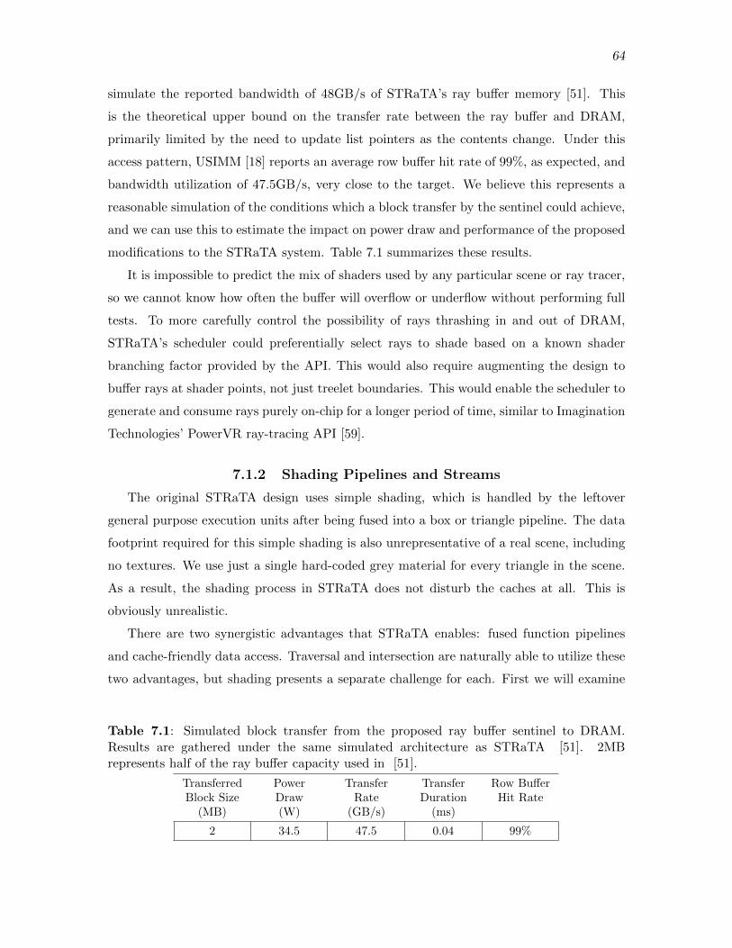
64
simulate the reported bandwidth of 48GB/s of STRaTA’s ray bu↵er memory [51]. This
is the theoretical upper bound on the transfer rate between the ray bu↵er and DRAM,
primarily limited by the need to update list pointers as the contents change. Under this
access pattern, USIMM [18] reports an average row bu↵er hit rate of 99%, as expected, and
bandwidth utilization of 47.5GB/s, very close to the target. We believe this represents a
reasonable simulation of the conditions which a block transfer by the sentinel could achieve,
and we can use this to estimate the impact on power draw and performance of the proposed
modifications to the STRaTA system. Table 7.1 summarizes these results.
It is impossible to predict the mix of shaders used by any particular scene or ray tracer,
so we cannot know how often the bu↵er will overflow or underflow without performing full
tests. To more carefully control the possibility of rays thrashing in and out of DRAM,
STRaTA’s scheduler could preferentially select rays to shade based on a known shader
branching factor provided by the API. This would also require augmenting the design to
bu↵er rays at shader points, not just treelet boundaries. This would enable the scheduler to
generate and consume rays purely on-chip for a longer period of time, similar to Imagination
Technologies’ PowerVR ray-tracing API [59].
7.1.2 Shading Pipelines and Streams
The original STRaTA design uses simple shading, which is handled by the leftover
general purpose execution units after being fused into a box or triangle pipeline. The data
footprint required for this simple shading is also unrepresentative of a real scene, including
no textures. We use just a single hard-coded grey material for every triangle in the scene.
As a result, the shading process in STRaTA does not disturb the caches at all. This is
obviously unrealistic.
There are two synergistic advantages that STRaTA enables: fused function pipelines
and cache-friendly data access. Traversal and intersection are naturally able to utilize these
two advantages, but shading presents a separate challenge for each. First we will examine
Table 7.1: Simulated block transfer from the proposed ray bu↵er sentinel to DRAM.Results are gathered under the same simulated architecture as STRaTA [51]. 2MBrepresents half of the ray bu↵er capacity used in [51].
TransferredBlock Size
(MB)
PowerDraw(W)
TransferRate
(GB/s)
TransferDuration(ms)
Row Bu↵erHit Rate
2 34.5 47.5 0.04 99%
65
the data coherence advantage. The bulk of data that a shader must access are typically
textures or other data that are treated as a texture, such as bump maps or displacement
maps. Luckily, existing graphics hardware has highly optimized custom texture support,
including texture caches. Although little is known about their implementation, it is unlikely
that any “treelet”-style clustering would improve their data access performance [35]. We
will therefore assume texture data in STRaTA would be handled by such hardware. The
remaining data associated with a shader should be relatively small, including a di↵use,
ambient, and specular color, shader type, texture ID, etc. This data should fit within the
16KB capacity of STRaTA’s L1 cache, requiring no thrashing for any given shader.
The other advantage of STRaTA, fused function pipelines, is made possible by the
bu↵ering of rays based on their category. Currently those categories are one of two: rays
performing box intersection, or rays performing triangle intersection. With a su�cient group
of rays ready to perform one type of action, the shared functional units can reconfigure in
to that pipeline mode. Without a critical mass of rays, reconfiguring the pipelines for just
one or two rays at a time would have very high overhead. In order to enable pipelines
for shading, one might consider creating new categories of ray bu↵ers, one for each shader
type, e.g., Lambertian, glass, cloth, etc. After a ray has passed through the traversal and
intersection phases, it could be placed in a new bu↵er for the corresponding material shader
that was hit, and the scheduler will eventually select a thread multiprocessor (TM) to shade
those rays.
Unlike traversal and intersection, the requirements for shading are very unpredictable,
and can vary drastically from scene to scene. In fact, it is impossible to predict what any
given shader may do, such as for one particular special e↵ect for a movie [29]. Shaders are
by nature programmable, but there are common themes throughout most shaders, such as
a high occurrence of 3D vector operations including normalization, reciprocal, addition and
subtraction, multiplication by a scalar, dot product, cross product, and many others. For
example a Lambertian, glass, and metal shader all use dot product, and many of the other
simple operations listed. We could construct full pipelines for the common shaders like
Lambertian, but without prior knowledge of the shaders to be executed, it is impossible to
accommodate them all. For this reason we propose creating functional unit configuration
modes with multiple common operations. Perhaps one mode would consist of two dot
product units and a vector addition/subtraction unit. This would tie up 6 multipliers and
2 adders for the dot products, and 3 adders for the add/sub unit. Under the baseline TRaX
configuration, this would leave 2 multipliers and 3 adders for general purpose use. Table 3.2
66
summarizes the potential benefits for a variety of common 3D vector operations. With
the right intelligent mixture of 3D vector operations, along with simpler multiply-add style
fusion, advanced shaders should see significant energy reductions. Di↵erent shaders may
be more amenable to di↵erent mixtures of units. The STRaTA system could o↵er multiple
di↵erent mixtures for di↵erent purposes, avoiding becoming overly shader specific.
7.1.3 Storing Shader State
Since a single ray cast in STRaTA is a non-blocking operation that may be shared by
multiple processors, any state associated with that ray, or any result that it may produce,
must be stored with the ray so it can be later accessed for shading. For example, a pixel ID
must be stored with every ray generated so that when shading is ultimately performed, the
correct pixel value can be set. When path tracing with Lambertian materials only, the extra
shading state that must be stored is quite simple, and consumes 48B in STRaTA [50]. This
takes advantage of many assumptions that are built in to the algorithm, such as knowing
that only one global illumination ray must be cast per shading point, so we don’t need to
keep track of how many more rays must be generated. In contrast, an ambient occlusion
shader may cast many rays per shade point [4], and we would need to store a counter with
each ray so that we know when to stop generating them. In this particular example, the
counter could be fairly small (just a few bits), but in general, we can not make assumptions
about a ray’s required shading state.
Laine et al. discuss wavefront path tracing [54], which has a similar requirement that
rays must be saved in memory instead of in registers, so that they may be passed among
multiple processing kernels. The paper specifically addresses di�culties that arise when
complex shaders are involved, including a 4-layer glossy car paint, noise-based procedural
displacement maps, tinted glass, and di↵use+glossy surfaces. The total state for each ray
path to handle complex shading of this nature is 212B, or 4.4⇥ larger than that required
in STRaTA.
Increasing the size of each ray results in a corresponding reduction in the number of
them that can be stored in on-chip bu↵ers. This reduction could potentially impact the
performance of the STRaTA system, since a certain critical mass of rays is required to
overcome the overheads of treelet processing. Data shows that STRaTA can tolerate a 2⇥
reduction in the number of rays in flight (equivalent to a 2⇥ increase in ray size) with little
impact on the energy advantage over the baseline [51]. Even a 4⇥ reduction in active rays
does not eliminate STRaTA’s energy advantage, and on some scenes it remains high. There
67
is a performance penalty in terms of rays/second, ranging between 7% to 31%, depending
on the scene, when the number of active rays is reduced fourfold.
Researchers have proposed hardware compression techniques to e↵ectively increase the
capacity or e�ciency of caches [76], and memory [1, 86], which would likely prove useful
for increasing the number of rays in flight in a STRaTA-like system. Specific context-aware
data organization may also be e↵ective, for example unit vectors need not consume three
full 32-bit words [21]. A combination of ray data compression and intelligent DRAM spilling
should allow STRaTA to handle arbitrary shading.
7.2 ConclusionRay-tracing has already become prevalent in o✏ine rendering systems, due to its ease
of use for high quality lighting simulation. We believe as processor technology continues
to advance, if pushed in the right direction, ray-tracing will become prevalent in real-time
systems as well. This dissertation addresses the high costs of data movement in processor
designs, and explores techniques for reducing those costs for ray-tracing in terms of energy
and time. For some applications, rays per second performance is the ultimate goal, so it may
be tempting to overlook energy consumption; however, energy can be the limiting factor
for improvements in processor performance. In the mobile domain, energy consumption is
elevated to a primary concern, where finite battery capacity determines the usefulness of
an energy-hungry application.
We started by designing a baseline platform called TRaX for exploring architectural
innovations for ray-tracing. The baseline is designed for ease of use and programmability
while achieving high performance in a small die-area budget. We then investigated the
data movement in this ray-tracing system, and characterized the associated energy costs.
We employ synergistic techniques that rethink the ray-tracing algorithm to reduce energy
consumption in the instruction fetch, register file, last-level cache, and o↵-chip DRAM
by reordering data accesses and rerouting compute kernel operands, without sacrificing
performance. Next, we closely examined the nature of DRAM and the importance of
modeling its subtle complexities in a simulator, particularly since it can be the performance
bottleneck and largest consumer of energy. We reveal that the way in which DRAM is
accessed can have a bigger impact on a ray-tracing system than the number of accesses.
Finally, we exploit the behavior of DRAM by even further modifying data access patterns
in our streaming ray tracer system. The result is a ray-tracing algorithm/architecture with
68
a substantial reduction in energy consumption, and a vast improvement in performance
scalability over basic architectures.
The STRaTA design presented demonstrates two improvements for ray-tracing that can
be applied to throughput-oriented architectures. First, we provide a memory architec-
ture to support smart ray reordering when combined with software that implements BVH
treelets. By deferring ray computations via streaming rays through intelligently blocked
and reordered data, we greatly increase cache hit rates, and improve the o↵-chip memory
access patterns, resulting in row bu↵er hit rates increasing from 35% to 80% in the best
case, DRAM energy up to 43% lower, and DRAM read latencies up to 85% faster. Second,
STRaTA allows shared XUs to be dynamically reconfigured into phase-specific pipelines
to support the dominant computational kernel for a particular treelet type. When these
phase-specific pipelines are active, they reduce instruction fetch and register usage by up
to 28%. If we combine the treelet streaming and phase-specific pipeline enhancements, we
see a total system-wide reduction in energy (including all caches, DRAM, register files, and
compute) of up to 30%.
By understanding and taking advantage of DRAM behavior, we are able to much more
e↵ectively utilize its available bandwidth, reducing or eliminating the primary performance
bottleneck. STRaTA is able to feed many more compute resources with data than a baseline
system, enabling performance to better scale with the number of cores. While the baseline
system’s performance peaks between 120 - 200 cores due to DRAM starvation, STRaTA
continues to improve up to 320 cores and beyond, achieving up to 100% higher performance.
REFERENCES
[1] Abali, B., Franke, H., Poff, D. E., Saccone Jr., R. A., Schulz, C. O.,Herger, L. M., and Smith, T. B. Memory expansion technology (MXT): Softwaresupport and performance. In IBM JRD (2001).
[2] Aila, T., and Karras, T. Architecture considerations for tracing incoherent rays.In Proc. High Performance Graphics (2010).
[3] Aila, T., Karras, T., and Laine, S. On quality metrics of bounding volumehierarchies. In Proc. High-Performance Graphics (2013).
[4] Aila, T., and Laine, S. Understanding the e�ciency of ray traversal on gpus. InProc. High Performance Graphics (2009).
[5] Aila, T., Laine, S., and Karras, T. Understanding the e�ciency of ray traversalon GPUs – Kepler and Fermi addendum. NVIDIA Technical Report NVR-2012-02,NVIDIA Corporation, June 2012.
[6] AMD. 3DNow! Technology Manual. http://support.amd.com/TechDocs/21928.pdf,2000.
[7] Behr, D. AMD GPU Architecture. In PPAM Tutorials (2009).
[8] Benthin, C., Wald, I., Woop, S., Ernst, M., and Mark, W. Combining singleand packet-ray tracing for arbitrary ray distributions on the intel mic architecture.Visualization and Computer Graphics, IEEE Transactions on 18, 9 (Sept 2012), 1438–1448.
[9] Bigler, J., Stephens, A., and Parker, S. G. Design for parallel interactive raytracing systems. In Symposium on Interactive Ray Tracing (IRT06) (2006).
[10] Bikker, J., and van Schijndel, J. The brigade renderer: A path tracer forreal-time games. In International Journal of Computer Games Technology (2013),vol. 2013.
[11] Bose, P. The power of communication. Keynote talk, WETI2012, 2012.
[12] Boulos, S., Edwards, D., Lacewell, J. D., Kniss, J., Kautz, J., Shirley,P., and Wald, I. Packet-based Whitted and Distribution Ray Tracing. In Proc.Graphics Interface (May 2007).
[13] Boulos, S., Wald, I., and Benthin, C. Adaptive ray packet reordering. InSymposium on Interactive Ray Tracing (IRT08) (2008).
[14] Brownlee, C., Fogal, T., and Hansen, C. D. GLuRay: Enhanced ray tracing inexisting scientific visualization applications using OpenGL interception. In EGPGV(2012), Eurographics, pp. 41–50.

70
[15] Brownlee, C., Ize, T., and Hansen, C. D. Image-parallel ray tracing usingOpenGL interception. In EGPGV (2013), Eurographics, pp. 65–72.
[16] Brunvand, E. High performance ray tracing: Implications for system architectures.Keynote talk, VLSI-SoC, 2012.
[17] Catmull, E. E. A Subdivision Algorithm for Computer Display of Curved Surfaces.PhD thesis, University of Utah, 1974.
[18] Chatterjee, N., Balasubramonian, R., Shevgoor, M., Pugsley, S., Udipi,A., Shafiee, A., Sudan, K., Awasthi, M., and Chishti, Z. USIMM: the UtahSImulated Memory Module. Tech. Rep. UUCS-12-02, University of Utah, 2012. Seealso: http://utaharch.blogspot.com/2012/02/usimm.html.
[19] Chris Lattner and Vikram Adve. The LLVM Instruction Set and CompilationStrategy. Tech. Report UIUCDCS-R-2002-2292, CS Dept., Univ. of Illinois at Urbana-Champaign, Aug 2002.
[20] Christensen, P. H., Laur, D. M., Fong, J., Wooten, W. L., and Batali, D.Ray di↵erentials and multiresolution geometry caching for distribution ray tracing incomplex scenes. In Eurographics (2003), pp. 543–552.
[21] Cigolle, Z. H., Donow, S., Evangelakos, D., Mara, M., McGuire, M.,and Meyer, Q. A survey of e�cient representations for independent unit vectors.Journal of Computer Graphics Techniques (JCGT) 3, 2 (April 2014), 1–30.
[22] Dachille, IX, F., and Kaufman, A. Gi-cube: an architecture for volumetric globalillumination and rendering. In ACM SIGGRAPH/EUROGRAPHICS Workshop onGraphics Hardware (2000), HWWS ’00, pp. 119–128.
[23] Dally, B. The challenge of future high-performance computing. Celsius Lecture,Uppsala University, Uppsala, Sweden, 2013.
[24] Davis, W., Zhang, N., Camera, K., Chen, F., Markovic, D., Chan, N.,Nikolic, B., and Brodersen, R. A design environment for high throughput,low power dedicated signal processing systems. In Custom Integrated Circuits, IEEEConference on. (2001), pp. 545–548.
[25] DWARF Debugging Information Format Committee. DWARF debugginginformation format version 4. http://www.dwarfstd.org/doc/DWARF4.pdf, 2010.
[26] Eisenacher, C., Nichols, G., Selle, A., and Burley, B. Sorted deferredshading for production path tracing. In Proceedings of the Eurographics Symposiumon Rendering (Aire-la-Ville, Switzerland, Switzerland, 2013), EGSR ’13, EurographicsAssociation, pp. 125–132.
[27] Ernst, M., and Greiner, G. Multi bounding volume hierarchies. In Symposiumon Interactive Ray Tracing (IRT08) (2008), pp. 35–40.
[28] Fajardo, M. Private Communication.
[29] Fajardo, M. How ray tracing conquered cinematic rendering. Keynote talk, HighPerformance Graphics, 2014.
[30] Glassner, A., Ed. An introduction to ray tracing. Academic Press, London, 1989.
71
[31] Govindaraju, V., Djeu, P., Sankaralingam, K., Vernon, M., and Mark,W. R. Toward a multicore architecture for real-time ray-tracing. In IEEE/ACMMicro ’08 (October 2008).
[32] Govindaraju, V., Djeu, P., Sankaralingam, K., Vernon, M., and Mark,W. R. Toward a multicore architecture for real-time ray-tracing. In IEEE/ACMInternational Conference on Microarchitecture (October 2008).
[33] Gribble, C., and Ramani, K. Coherent ray tracing via stream filtering. InSymposium on Interactive Ray Tracing (IRT08) (2008).
[34] Gunther, J., Popov, S., Seidel, H.-P., and Slusallek, P. Realtime ray tracingon GPU with BVH-based packet traversal. In Symposium on Interactive Ray Tracing(IRT07) (2007), pp. 113–118.
[35] Hakura, Z. S., and Gupta, A. The design and analysis of a cache architecturefor texture mapping. In Proceedings of the 24th Annual International Symposium onComputer Architecture (1997), ISCA ’97, ACM, pp. 108–120.
[36] Hameed, R., Qadeer, W., Wachs, M., Azizi, O., Solomatnikov, A., Lee,B. C., Richardson, S., Kozyrakis, C., and Horowitz, M. Understandingsources of ine�ciency in general-purpose chips. In Proceedings of the 37th AnnualInternational Symposium on Computer Architecture (2010), ISCA ’10, ACM, pp. 37–47.
[37] Hapala, M., Davidovic, T., Wald, I., Havran, V., and Slusallek, P.E�cient Stack-less BVH Traversal for Ray Tracing. In Proceedings 27th SpringConference of Computer Graphics (SCCG) (2011), pp. 29–34.
[38] HWRT. SimTRaX a cycle-accurate ray tracing architectural simulator and compiler.http://code.google.com/p/simtrax/, 2012. Utah Hardware Ray Tracing Group.
[39] Ibrahim, A., Parker, M., and Davis, A. Energy E�cient Cluster Co-Processors.In Proceedings of the International Conference on Acoustics, Speech, and SignalProcessing (2004).
[40] Imagination Technologies. MIPS architectures. http://www.imgtec.com/mips/architectures/, 2015.
[41] Imagination Technologies. MIPS SIMD. http://www.imgtec.com/mips/architectures/simd.asp, 2015.
[42] Intel. Intel SSE4 Programming Reference. https://software.intel.com/sites/default/files/c8/ab/17971-intel 20sse4 20programming 20reference.pdf, 2007.
[43] Intel. Intel 64 and IA-32 Architectures Software Developer’s Manual.http://www.intel.com/content/dam/www/public/us/en/documents/manuals/64-ia-32-architectures-software-developer-vol-1-manual.pdf, 2014.
[44] Ize, T. E�cient Acceleration Structures for Ray Tracing Static and Dynamic Scenes.PhD thesis, The University of Utah, August 2009.
[45] Ize, T., Brownlee, C., and Hansen, C. D. Real-time ray tracer for visualizingmassive models on a cluster. In EGPGV (2011), Eurographics, pp. 61–69.
72
[46] Jacob, B., Ng, S. W., and Wang, D. T. Memory Systems - Cache, DRAM, Disk.Elsevier, 2008.
[47] Kajiya, J. T. The rendering equation. In Proceedings of SIGGRAPH (1986),pp. 143–150.
[48] Keely, S. Reduced precision for hardware ray tracing in GPUs. In High-PerformanceGraphics (HPG 2014) (2014).
[49] Kim, H.-Y., Kim, Y.-J., and Kim, L.-S. MRTP: Mobile ray tracing processor withreconfigurable stream multi-processors for high datapath utilization. IEEE Journalof Solid-State Circuits 47, 2 (feb. 2012), 518–535.
[50] Kopta, D., Shkurko, K., Spjut, J., Brunvand, E., and Davis, A. An energyand bandwidth e�cient ray tracing architecture. In High-Performance Graphics(HPG 2013) (2013).
[51] Kopta, D., Shkurko, K., Spjut, J., Brunvand, E., and Davis, A. Memoryconsiderations for low-energy ray tracing. Computer Graphics Forum (2014).
[52] Kopta, D., Spjut, J., Brunvand, E., and Davis, A. E�cient MIMD archi-tectures for high-performance ray tracing. In IEEE International Conference onComputer Design (ICCD) (2010).
[53] Laine, S. Restart trail for stackless BVH traversal. In Proc. High PerformanceGraphics (2010), pp. 107–111.
[54] Laine, S., Karras, T., and Aila, T. Megakernels considered harmful: Wavefrontpath tracing on GPUs. In Proc. High Performance Graphics (2013).
[55] Lindholm, E., Nickolls, J., Oberman, S., and Montrym, J. NVIDIA Tesla: Aunified graphics and computing architecture. Micro, IEEE 28, 2 (March-April 2008),39–55.
[56] Luitjens, J., and Rennich, S. CUDA Warps and Occupancy, 2011. GPUComputing Webinar.
[57] Mansson, E., Munkberg, J., and Akenine-Moller, T. Deep coherent raytracing. In Symposium on Interactive Ray Tracing (IRT07) (2007).
[58] Mathew, B., Davis, A., and Parker, M. A Low Power Architecture forEmbedded Perception Processing. In Proceedings of the International Conferenceon Compilers, Architecture, and Synthesis for Embedded Systems (2004), pp. 46–56.
[59] McCombe, J. Introduction to PowerVR ray tracing. GDC, 2014.
[60] Moller, T., and Trumbore, B. Fast, minimum storage ray triangle intersection.Journal of Graphics Tools 2, 1 (October 1997), 21–28.
[61] Moon, B., Byun, Y., Kim, T.-J., Claudio, P., Kim, H.-S., Ban, Y.-J., Nam,S. W., and Yoon, S.-E. Cache-oblivious ray reordering. ACM Trans. Graph. 29, 3(July 2010), 28:1–28:10.
[62] MSC. 2012 Memory Scheduling Championship, 2012. http://www.cs.utah.edu/⇠rajeev/jwac12/.

73
[63] Muralimanohar, N., Balasubramonian, R., and Jouppi, N. OptimizingNUCA organizations and wiring alternatives for large caches with CACTI 6.0. InMICRO ’07 (2007), pp. 3–14.
[64] Nah, J.-H., Kim, J.-W., Park, J., Lee, W.-J., Park, J.-S., Jung, S.-Y., Park,W.-C., Manocha, D., and Han, T.-D. Hart: A hybrid architecture for ray tracinganimated scenes. Visualization and Computer Graphics, IEEE Transactions on 21, 3(March 2015), 389–401.
[65] Nah, J.-H., Park, J.-S., Park, C., Kim, J.-W., Jung, Y.-H., Park, W.-C., andHan, T.-D. T&I engine: Traversal and intersection engine for hardware acceleratedray tracing. In Proceedings of the 2011 SIGGRAPH Asia Conference (New York, NY,USA, 2011), SA ’11, ACM, pp. 160:1–160:10.
[66] Nair, P., Chou, C.-C., and Qureshi, M. K. A case for refresh pausing in DRAMmemory systems. In IEEE Symposium on High Performance Computer Architecture(HPCA) (2013), HPCA ’13, IEEE Computer Society, pp. 627–638.
[67] Navratil, P., Fussell, D., Lin, C., and Mark, W. Dynamic ray scheduling forimproved system performance. In Symposium on Interactive Ray Tracing (IRT07)(2007).
[68] Navratil, P. A., and Mark, W. R. An analysis of ray tracing bandwidthconsumption. Tech. Rep. TR-06-40, The University of Texas at Austin, 2006.
[69] NVIDIA. GeForce GTX 200 GPU architectural overview. Tech. Rep. TB-04044-001 v01, NVIDIA Corporation, May 2008.
[70] NVIDIA. NVIDIA GeForce GTX 980. White Paper, 2014. http://international.download.nvidia.com/geforce-com/international/pdfs/GeForceGTX 980 Whitepaper FINAL.PDF.
[71] NVIDIA CUDA Documentation. http://developer.nvidia.com/object/cuda.html.
[72] O, S., Son, Y. H., Kim, N. S., and Ahn, J. H. Row-bu↵er decoupling: A case forlow-latency dram microarchitecture. In Proceeding of the 41st Annual InternationalSymposium on Computer Architecuture (2014), ISCA ’14, IEEE Press, pp. 337–348.
[73] Overbeck, R., Ramamoorthi, R., and Mark, W. R. Large ray packets forreal-time whitted ray tracing. In Symposium on Interactive Ray Tracing (IRT08)(2008), pp. 41–48.
[74] Parker, S., Martin, W., Sloan, P.-P., Shirley, P., Smits, B., and Hansen,C. Interactive ray tracing. In Symposium on Interactive 3D Graphics: Interactive 3D(April 26-28 1999), pp. 119–126.
[75] Parker, S. G., Bigler, J., Dietrich, A., Friedrich, H., Hoberock, J.,Luebke, D., McAllister, D., McGuire, M., Morley, K., Robison, A., andStich, M. OptiX: a general purpose ray tracing engine. In ACM SIGGRAPH papers(2010), SIGGRAPH ’10, ACM, pp. 66:1–66:13.
[76] Pekhimenko, G., Seshadri, V., Mutlu, O., Mowry, T. C., Gibbons, P. B.,and Kozuch, M. A. Base-delta-immediate compression: A practical data compres-sion mechanism for on-chip caches. In Proceedings of PACT (2012).

74
[77] Pharr, M., and Hanrahan, P. Geometry caching for ray-tracing displacementmaps. In Eurographics Rendering Workshop (1996), pp. 31–40.
[78] Pharr, M., Kolb, C., Gershbein, R., and Hanrahan, P. Rendering complexscenes with memory-coherent ray tracing. In SIGGRAPH ’97 (1997), pp. 101–108.
[79] Purcell, T. J., Buck, I., Mark, W. R., and Hanrahan, P. Ray tracingon programmable graphics hardware. ACM Transactions on Graphics 21, 3 (2002),703–712.
[80] Ramani, K. CoGenE: An Automated Design Framework for Domain Specific Archi-tectures. PhD thesis, University of Utah, October 2012.
[81] Ramani, K., and Davis, A. Application driven embedded system design: a facerecognition case study. In International Conference on Compilers, Architecture andSynthesis for Embedded Systems (CASES) (Salzburg, Austria, 2007).
[82] Ramani, K., and Gribble, C. StreamRay: A stream filtering architecture forcoherent ray tracing. In ASPLOS ’09 (2009).
[83] Rixner, S., Dally, W. J., Kapasi, U. J., Mattson, P., and Owens, J. D.Memory access scheduling. SIGARCH Comput. Archit. News 28, 2 (May 2000), 128–138.
[84] Schmittler, J., Wald, I., and Slusallek, P. SaarCOR – A Hardware Archi-tecture for Realtime Ray-Tracing. In Proceedings of EUROGRAPHICS Workshop onGraphics Hardware (2002).
[85] Schmittler, J., Woop, S., Wagner, D., Paul, W. J., and Slusallek, P.Realtime ray tracing of dynamic scenes on an FPGA chip. In Graphics HardwareConference (August 2004), pp. 95–106.
[86] Shafiee, A., Taassori, M., Balasubramonian, R., and Davis, A. Memzip:Exploring unconventional benefits from memory compression. In High PerformanceComputer Architecture (HPCA), 2014 IEEE 20th International Symposium on (Feb2014), pp. 638–649.
[87] Shebanow, M. An evolution of mobile graphics. Keynote talk, High PerformanceGraphics, 2013.
[88] Shevtsov, M., Soupikov, A., Kapustin, A., and Novorod, N. Ray-TriangleIntersection Algorithm for Modern CPU Architectures. In Procedings of Graph-iCon’2007 (Moscow, Russia, June 2007).
[89] Shirley, P., and Morley, R. K. Realistic Ray Tracing. A. K. Peters, Natick,MA, 2003.
[90] Silicon Arts Coproration. RayCore series 1000, 2013. http://www.siliconarts.co.kr/gpu-ip.
[91] Smits, B. E�ciency issues for ray tracing. J. Graph. Tools 3, 2 (Feb. 1998), 1–14.
[92] Spjut, J. E�cient Ray Tracing Architectures. PhD thesis, University of Utah,December 2013.

75
[93] Spjut, J., Kensler, A., Kopta, D., and Brunvand, E. TRaX: A multicorehardware architecture for real-time ray tracing. IEEE Transactions on Computer-Aided Design 28, 12 (2009), 1802 – 1815.
[94] Spjut, J., Kopta, D., Boulos, S., Kellis, S., and Brunvand, E. TRaX: Amulti-threaded architecture for real-time ray tracing. In 6th IEEE Symposium onApplication Specific Processors (SASP) (June 2008).
[95] Steinhurst, J., Coombe, G., and Lastra, A. Reordering for cache consciousphoton mapping. In Proceedings of Graphics Interface (2005), pp. 97–104.
[96] Stone, J. E., Gohara, D., and Shi, G. Opencl: A parallel programming standardfor heterogeneous computing systems. IEEE Des. Test 12, 3 (May 2010), 66–73.
[97] Tsakok, J. A. Faster incoherent rays: Multi-BVH ray stream tracing. In Proc. HighPerformance Graphics (2009), pp. 151–158.
[98] Udipi, A. N., Muralimanohar, N., Chatterjee, N., Balasubramonian, R.,Davis, A., and Jouppi, N. P. Rethinking DRAM design and organization forenergy-constrained multi-cores. In Proceedings of the 37th Annual InternationalSymposium on Computer Architecture (2010), ISCA ’10, ACM, pp. 175–186.
[99] Wald, I., Benthin, C., and Boulos, S. Getting rid of packets - e�cient SIMDsingle-ray traversal using multi-branching BVHs. In Symposium on Interactive RayTracing (IRT08) (2008), pp. 49–57.
[100] Wald, I., Purcell, T. J., Schmittler, J., and Benthin, C. Realtime raytracing and its use for interactive global illumination. In In Eurographics State of theArt Reports (2003).
[101] Wald, I., Slusallek, P., Benthin, C., and Wagner, M. Interactive renderingwith coherent ray tracing. Computer Graphics Forum (EUROGRAPHICS ’01) 20, 3(2001), 153–164.
[102] Wald, I., Woop, S., Benthin, C., Johnson, G. S., and Ernst, M. Embree- a kernel framework for e�cient CPU ray tracing. In ACM SIGGRAPH (2014),SIGGRAPH ’14, ACM.
[103] Whitted, T. An improved illumination model for shaded display. Communicationsof the ACM 23, 6 (1980), 343–349.
[104] Williams, A., Barrus, S., Morley, R. K., and Shirley, P. An e�cient androbust ray-box intersection algorithm. Journal of Graphics Tools 10, 1 (2005).
[105] Woop, S., Brunvand, E., and Slusallak, P. Estimating performance of a raytracing ASIC design. In IRT06 (Sept. 2006).
[106] Woop, S., Schmittler, J., and Slusallek, P. RPU: A programmable rayprocessing unit for realtime ray tracing. ACM Transactions on Graphics (SIGGRAPH’05) 24, 3 (July 2005).
[107] Xilinx. Microblaze processor reference guide. reference manual (2006), 23.