Ray synthetic seismograms for a 3-D anisotropic …seis.karlov.mff.cuni.cz/papers.bin/a88ip1.pdf · each elementary wave and each receiver position 3. Ray synthetic seismograms for

Physics of the Earth and Planetary Interiors, 51 (1988) 1-23 Elsevier Science Publishers B.V., Amsterdam - Printed in The Netherlands

Ray synthetic seismograms for a 3-D anisotropic lithospheric structure

D. Gajewski

Geophysical Institute, Karlsruhe University, Hertzstrasse 16, 7500 Karlsruhe- West (F.R.G.)

Geophysical Institute, Czechoslouak Academy of Sciences, Bdni 11, 141 31 Praha 4 (Czechoslovakia)

(Received October 31,1986; revision accepted March 28, 1987)

Gajewski, D. and PSenEik, I., 1988. Ray synthetic seismograms for a 3-D anisotropic lithospheric structure. Phys. Earth Planet. Inter.. 51: 1-23.

The ray method is a useful tool for investigating the effects of anisotropy and inhomogeneity on the propagation of high-frequency seismic wave fields in elastic media. A program, based on the ray method, has been written to compute synthetic seismograms for 3-D laterally inhomogeneous media composed of isotropic and anisotropic inhomogeneous layers. General anisotropy, which can be described by 21 independent elastic parameters, may be considered by this program. Ray paths and travel times are evaluated by numerically integrating the corresponding ray tracing equations. When computing amplitudes, an approximate value of the geometrical spreading is obtained by numerically calculating the cross-sectional area of a ray tube. A paraxial ray approximation is used to evaluate the computed wave field in the vicinity of termination points of the rays. If a sufficiently dense system of ray-termination points covers a region on the surface of the model, synthetic seismograms along an arbitrary profile, fan or array in that region can be computed. In this paper, the effects of anisotropy on the propagation of elastic waves in a structure which simulates a continental subcrustal lithosphere are studied and P- and S-wave synthetic record sections along several profiles and fans are presented and discussed.

1. Introduction

Elastic anisotropy in the Earth's crust and the upper mantle is a commonly accepted and well- documented fact. Observed azimuthal dependence of travel times of refracted waves in some regions or shear wave splitting can be taken as indications of this. Anisotropy may be caused by many fac- tors including stress, crystal alignment, equally oriented cracks and thin layering. In this paper, rather than investigate the causes of anisotropy, we will concentrate on how it affects seismic wave propagation. In the real Earth, the effects of anisotropy are combined with the effects of inhomo- geneities. To understand these effects, and, possi-

bly, to find ways to separate them, numerical modelling of seismic wave propagation in laterally inhomogeneous anisotropic structures is necessary.

In recent years, various methods for the computation of seismic wave fields in anisotropic media have been suggested. A modified reflectivity method has been used for this purpose by Crampin and hls colleagues (for references see Crampin (1981)), or more recently by Gruenewald (1986). The Alekseyev-Mikhailenko method has also been applied to anisotropic media. For references on this topic see the review paper by Mikhailenko (1985).

Various high-frequency asymptotic methods,

0031-9201/88/$03.50 0 1988 Elsevier Science Publishers B.V.

whlch proved to be valuable when applied to inhomogeneous isotropic structures, appear to be a very promising way of approaching this problem. Under the assumption of slow variation of wave and medium parameters within a wave- length, these methods can be applied to a broad variety of rather complex models of 3-D laterally varying layered anisotropic structures, which may be difficult to investigate by other more exact methods. One of the greatest attributes of the high-frequency asymptotic methods compared with the above mentioned algorithms is their com- putational efficiency, which makes it possible to use the high-frequency asymptotic methods for routine interpretations. Another important prop- erty of these methods is that it is possible to single out individual parts of the total wave field, and thus give a clearer insight into how these individual, identifiable arrivals contribute to the total wave field.

It should also be mentioned that some attempts have been made to apply the Gaussian beam method to seismic wave propagation problems in inhomogeneous anisotropic media (Hanyga, 1986). In the following, we will concentrate on the ray method.

The first attempts to apply the ray method to the problem of the propagation of elastic waves in inhomogeneous anisotropic media were made by Babich (1961) and cervenjr (1972). The latter derived an easily programmed ray tracing system and a method which is now known as dynamic ray tracing for general inhomogeneous anisotropic media. However, these systems were for the most part applied only to simplified types of media and propagation problems; specifically in the computation of travel times of seismic waves propagating in a symmetry plane of a 2-D vertically inhomogeneous transversely isotropic medium (cervenjr and PSenEik, 1972). Another application of the theory derived by cervenjr (1972) was in a method based on linearized equations for computing travel times in weakly anisotropic laterally inhomogeneous media (cervenjr and Firbas, 1984).

In the program package used for the computation of synthetic seismograms presented in this paper, a general 3-D laterally varying layered medium composed of isotropic and anisotropic

layers can be considered. The approach is based on formulae derived by Babich (1961) and Cerven? (1972). No assumption of weak anisotropy, and thus no linearization, is used. On the contrary, the formulae used are preferable for application to media displaying strong anisotropy. With an accuracy comparable to that of zero-order asymptotic ray theory, the formulae accurately describe the propagation of quasi-P waves and also yield accurate results for travel times of quasi-S waves. They may, however, give distorted amplitudes and polarizations of the two quasi-S waves in cases where the phase velocities of these waves are almost equal (Kravtsov and Orlov, 1980). It is also necessary to keep in mind that since the ray method is used, limited accuracy of amplitudes near singular regions (such as the vicinity of caus- tics, cusp points and the boundaries of illuminated and shadow regions), and higher sensitivity of amplitudes to the approximation of the model should be expected.

In section 2, a short description is given of the models, sources and the algorithm used for the computation of seismic wave fields for such models. More details about the algorithm, and the program package based on the algorithm, may be found in Gajewski and PSenEik (1987). Numerical results simulating deep seismic sounding measure- ments in a region with an anisotropic upper mantle are presented in section 3. They consist of synthetic sections obtained along different straight profiles passing through the source (profile observations), and of sections obtained on concentric circles around the source (fan observations). Com- parison of numerical results and observed refraction seismic data is briefly discussed in section 4. Some practical implications, whch follow from the numerical tests performed, are given in the conclusion.

2. Description of the procedure for computing ray synthetic seismograms

2.1. Model, source and receivers

A 3-D model consisting of a system of layers separated by curved non-intersecting interfaces is

considered. The layers may be either isotropic or anisotropic. In general, inside the anisotropic layers all 21 elastic parameters and density may vary, while in the isotropic layers only the P- and S-wave velocities and density may vary. There are two possible ways that the elastic parameters may vary within the individual layers:

(1) variation of elastic parameters with depth only; and

(2) linear variation of elastic parameters along vertical lines between interfaces representing iso- surfaces of elastic parameters. In the former approach, the distribution of elastic parameters within the layers is laterally homoge- neous, and only the thicknesses of the layers may vary due to curved or inclined interfaces. In the latter approach, the distribution of elastic parameters is laterally varying inside layers if their boundaries are curved or inclined. The vertical gradient in a layer is higher if the interfaces bounding the layer are close to one another, and vice versa.

In the present version of the program, seismic waves are generated by a point source situated at any location within an isotropic layer. The point sources most frequently used in seismology, such as the explosive (implosive) source, the single force and the double couple point source, with a frequency-independent radiation pattern, are considered. For convenience, the Gaussian envelope signal is used as a source-time function. This makes fast approximate analytic evaluation of elementary ray synthetic seismograms possible (Cerven~ et al., 1977).

The receivers are expected to be situated on the Earth's surface, and may be arbitrarily distributed along profiles, fans or in arrays.

2.2. Computation of the seismic wave field

The procedure for evaluating the seismic wave field consists of two parts:

(1) kinematic part, computation of rays and travel times;

(2) dynamic part, computation of the geometrical spreading, reflection/transrnission coefficients and amplitudes.

For the computation of rays and travel times in

anisotropic layers, the ray tracing system given by Cerven~ (1972) is used, supplemented by proce- dures for the transformation of the slowness vector across interfaces separating anisotropic and/or isotropic layers (Fedorov, 1968). In isotropic layers, standard ray tracing (Cervenj, et al., 1977), is applied.

The evaluation of amplitudes in inhomogeneous anisotropic media is very similar to that in isotropic media. The most important quantities to be determined on each ray are the radiation pattern, the reflection/transmission and surface conversion coefficients, and the geometrical spreading. Since the source is situated in an isotropic layer, the determination of the radiation pattern is straightforward. To determine the coefficients of reflection and transmission, a system of six linear algebraic equations resulting from conditions of continuity of displacements and stresses across an interface must be solved at each interface (Fedorov, 1968). For surface conversion coefficients, the system reduces to three linear algebraic equations.

The geometrical spreading is obtained by a simple technique based on the direct measurement of the cross-sectional area of the ray tube, formed by three neighbouring rays, rather than numerically solving the complicated dynamic ray tracing system.

The results of kinematic and dynamic computations are travel times and complex vectorial amplitudes at termination points of the rays on the Earth's surface. To avoid time-consuming two- point ray tracing from the source to the receivers, we extrapolate the travel times and amplitudes to the receivers from the closest termination points. At present, a paraxial ray approximation is used to determine the travel times at receivers, and linear interpolation is used for the amplitudes. The formulae for the paraxial approximation are evaluated in a manner similar to that used for the geometrical spreading, which utilizes information from neighbouring rays (see Gajewski and PSenEik, 1987).

Once the travel times and complex vectorial amplitudes corresponding to different elementary waves are known at a receiver, the construction of a ray synthetic seismogram is straightforward. For

each elementary wave and each receiver position 3. Ray synthetic seismograms for a subcrustal an- an elementary ray synthetic seismogram is com- isotropic lithosphere puted. The final synthetic seismogram at a receiver is obtained as a superpositibn of the ele- The program package based on the procedure mentary ray seismograms. For this purpose, the described in the previous section was applied to program SYNTPL of the package SEIS83 (Cervenq study the seismic wave fields in a model of an and PSeniSik, 1984) is used. anisotropic continental subcrustal lithosphere, the

( b ) HORIZONTAL PHASE VELOCITIES IN KMlSEC

QUASI P WAVE QUASI S WAVES

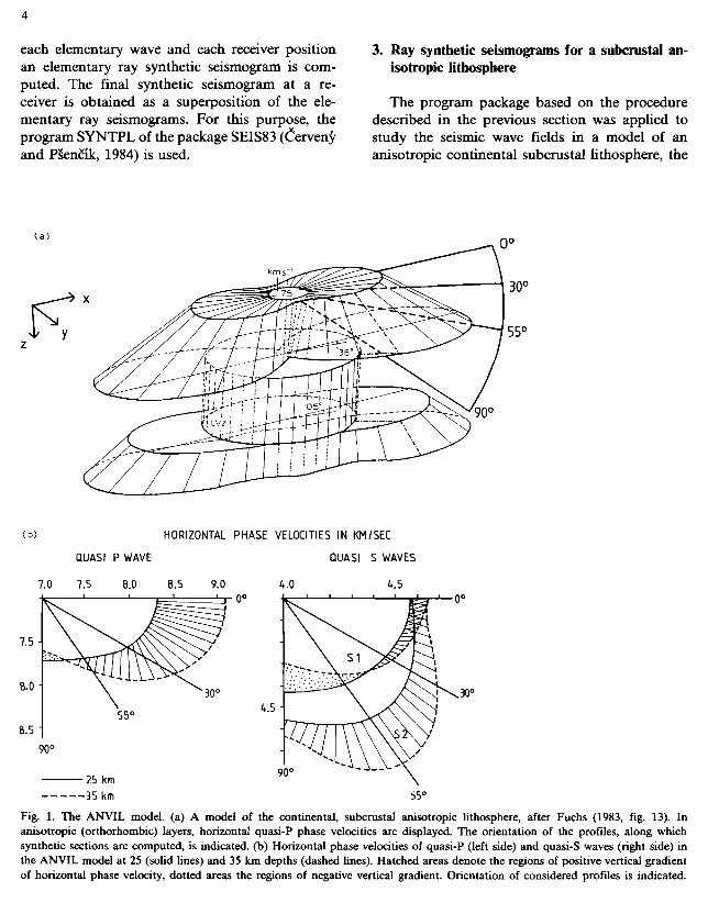
Fig. 1. The ANVIL model. (a) A model of the continental, subcrustal anisotropic lithosphere, after Fuchs (1983, fig. 13). In anisotropic (orthorhombic) layers, horizontal quasi-P phase velocities are displayed. The orientation of the profiles, along which synthetic sections are computed, is indicated. (b) Horizontal phase velocities of quasi-P (left side) and quasi-S waves (right side) in the ANVIL model at 25 (solid lines) and 35 km depths (dashed lines). Hatched areas denote the regions of positive vertical gradient of horizontal phase velocity, dotted areas the regions of negative vertical gradient. Orientation of considered profiles is indicated.

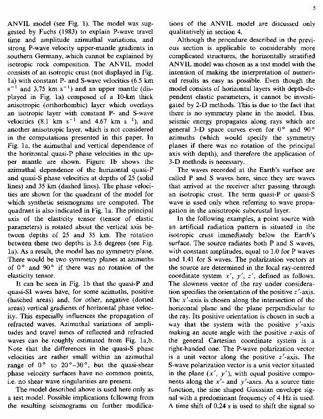
ANVIL model (see Fig. 1). The model was suggested by Fuchs (1983) to explain P-wave travel time and amplitude azimuthal variations, and strong P-wave velocity upper-mantle gradients in southern Germany, which cannot be explained by isotropic rock composition. The ANVIL model consists of an isotropic crust (not displayed in Fig. la) with constant P- and S-wave velocities (6.5 km s-I and 3.75 km s-') and an upper mantle (displayed in Fig. la) composed of a 10-km thick anisotropic (orthorhombic) layer whch overlays an isotropic layer with constant P- and S-wave velocities (8.1 km s-' and 4.67 km s-I), and another anisotropic layer, which is not considered in the computations presented in ths paper. In Fig. la, the azimuthal and vertical dependence of the horizontal quasi-P phase velocities in the upper mantle are shown. Figure l b shows the azimuthal dependence of the horizontal quasi-P and quasi-S phase velocities at depths of 25 (solid lines) and 35 km (dashed lines). The phase velocities are shown for the quadrant of the model for which synthetic seismograms are computed. The quadrant is also indicated in Fig. la. The principal axis of the elasticity tensor (tensor of elastic parameters) is rotated about the vertical axis between depths of 25 and 35 km. The rotation between these two depths is 3.6 degrees (see Fig. la). As a result, the model has no symmetry plane. There would be two symmetry planes at azimuths of 0" and 90" if there was no rotation of the elasticity tensor.

It can be seen in Fig. l b that the quasi-P and quasi-S1 waves have, for some azimuths, positive (hatched areas) and, for other, negative (dotted areas) vertical gradients of horizontal phase velocity. This especially influences the propagation of refracted waves. Azimuthal variations of amplitudes and travel times of reflected and refracted waves can be roughly estimated from Fig. la,b. Note that the differences in the quasi-S phase velocities are rather small within an azimuthal range of 0 " to 20 "-30 ", but the quasi-shear phase velocity surfaces have no common points, i.e. no shear wave singularities are present.

The model described above is used here only as a test model. Possible implications fcllowing from the resulting seismograms on further modifica-

tions of the ANVIL model are discussed only qualitatively in section 4.

Although the procedure described in the previous section is applicable to considerably more complicated structures, the horizontally stratified ANVIL model was chosen as a test model with the intention of making the interpretation of numerical results as easy as possible. Even though the model consists of horizontal layers with depth-dependent elastic parameters, it cannot be investi- gated by 2-D methods. This is due to the fact that there is no symmetry plane in the model. Thus, seismic energy propagates along rays which are general 3-D space curves even for 0" and 90" azimuths (which would specify the symmetry planes if there was no rotation of the principal axis with depth), and therefore the application of 3-D methods is necessary.

The waves recorded at the Earth's surface are called P and S waves here, since they are waves that arrived at the receiver after passing through an isotropic crust. The term quasi-P or quasi-S wave is used only when referring to wave propagation in the anisotropic subcrustal layer.

In the following examples, a point source with an artificial radiation pattern is situated in the isotropic crust immediately below the Earth's surface. The source radiates both P and S waves, with constant amplitudes, equal to 1.0 for P waves and 1.41 for S waves. The polarization vectors at the source are determined in the local ray-centred coordinate system x', y', z', defined as follows. The slowness vector of the ray under considera- tion specifies the orientation of the positive z'-axis. The x'-axis is chosen along the intersection of the horizontal plane and the plane perpendicular to the ray. Its positive orientation is chosen in such a way that the system with the positive y'-axis making an acute angle with the positive z-axis of the general Cartesian coordinate system is a right-handed one. The P-wave polarization vector is a unit vector along the positive z'-axis. The S-wave polarization vector is a unit vector situated in the plane (x', y'), with equal positive components along the x'- and yr-axes. As a source time function, the sine shaped Gaussian envelope signal with a predominant frequency of 4 Hz is used. A time shift of 0.24 s is used to shift the signal so

that arrival times correspond to the onset of the signal.

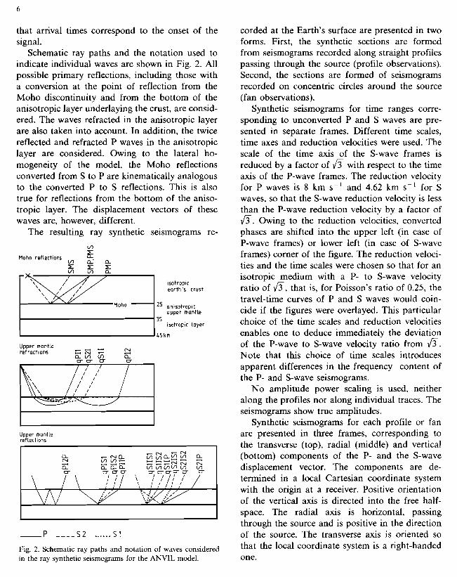
Schematic ray paths and the notation used to indicate individual waves are shown in Fig. 2. All possible primary reflections, including those with a conversion at the point of reflection from the Moho discontinuity and from the bottom of the anisotropic layer underlaying the crust, are considered. The waves refracted in the anisotropic layer are also taken into account. In addition, the twice reflected and refracted P waves in the anisotropic layer are considered. Owing to the lateral ho- mogeneity of the model, the Moho reflections converted from S to P are kinematically analogous to the converted P to S reflections. This is also true for reflections from the bottom of the anisotropic layer. The displacement vectors of these waves are, however, different.

The resulting ray synthetic seismograms re-

isotropic earth's crust

anisotrop~c upper mantle

isotropic layer

Upper mantle refract~ons L K j = ,, , E

\

c-- . ..-

Upper mantle reflections

Fig. 2. Schematic ray paths and notation of waves considered in the ray synthetic seismograms for the ANVIL model.

corded at the Earth's surface are presented in two forms. First, the synthetic sections are formed from seismograms recorded along straight profiles passing through the source (profile observations). Second, the sections are formed of seismograms recorded on concentric circles around the source (fan observations).

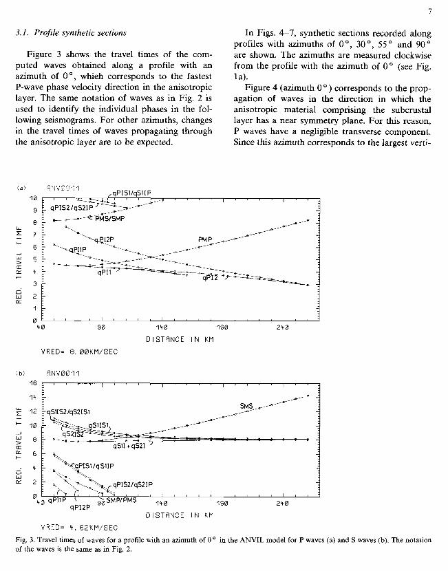
Synthetic seismograms for time ranges corresponding to unconverted P and S waves are presented in separate frames. Different time scales, time axes and reduction velocities were used. The scale of the time axis of the S-wave frames is reduced by a factor of 6 with respect to the time axis of the P-wave frames. The reduction velocity for P waves is 8 km s-' and 4.62 krn s-' for S waves, so that the S-wave reduction velocity is less than the P-wave reduction velocity by a factor of 6. Owing to the reduction velocities, converted phases are shifted into the upper left (in case of P-wave frames) or lower left (in case of S-wave frames) comer of the figure. The reduction velocities and the time scales were chosen so that for an isotropic medium with a P- to S-wave velocity ratio of 6, that is, for Poisson's ratio of 0.25, the travel-time curves of P and S waves would coin- cide if the figures were overlayed. This particular choice of the time scales and reduction velocities enables one to deduce immediately the deviation of the P-wave to S-wave velocity ratio from 6. Note that this choice of time scales introduces apparent differences in the frequency content of the P- and S-wave seismograms.

No amplitude power scaling is used, neither along the profiles nor along individual traces. The seismograms show true amplitudes.

Synthetic seismograms for each profile or fan are presented in three frames, corresponding to the transverse (top), radial (middle) and vertical (bottom) components of the P- and the S-wave displacement vector. The components are determined in a local Cartesian coordinate system with the origin at a receiver. Positive orientation of the vertical axis is directed into the free half- space. The radial axis is horizontal, passing through the source and is positive in the direction of the source. The transverse axis is oriented so that the local coordinate system is a right-handed one.

3.1. Profile synthetic sections

Figure 3 shows the travel times of the computed waves obtained along a profile with an azimuth of 0°, whieh corresponds to the fastest P-wave phase velocity direction in the anisotropic layer. The same notation of waves as in Fig. 2 is used to identify the individual phases in the following seismograms. For other azimuths, changes in the travel times of waves propagating through the anisotropic layer are to be expected.

In Figs. 4-7, synthetic sections recorded along profiles with azimuths of 0 O, 30 O, 55 and 90 " are shown. The azimuths are measured clockwise from the profile with the azimuth of 0" (see Fig. la).

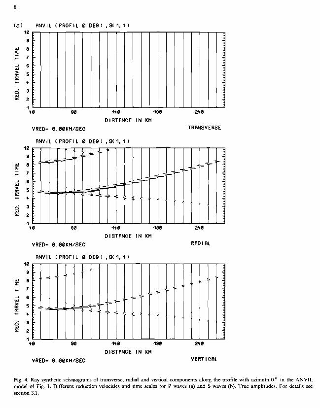
Figure 4 (azimuth 0 " ) corresponds to the propagation of waves in the direction in which the anisotropic material comprising the subcrustal layer has a near symmetry plane. For this reason, P waves have a neghgible transverse component. Since thls azimuth corresponds to the largest verti-

AbIVOO<'I I0

9

8

7

6

5

4

3

2

1

0 4 0 90 140 190 24 0

DISTANCE I N KM

VRED= 8. 00KM/SEC

DISTANCE I N KM

VRED= 4. 62KM/SEC

Fig. 3. Travel times of waves for a profile with an azimuth of 0 in the ANVIL model for P waves (a) and S waves (b). The notation of the waves is the same as in Fig. 2.

(a) R N V I L ( P R O F I L 0 D E G ) , S ( l , I )

DISTANCE I N KM

VRED- 8.00KM/SEC TRANSVERSE

ANVIL (PROFIL 0 DEG) , S ( I , I ) 10

1 4 0 90 14B I90 24 0

DISTANCE I N KM

VRED- 8. 00KM/SEC RRD l AL

ANVIL (PROFIL 0 DEO) , S ( 1 , 1 ) 40

9

I 4 0 80 I+0 198 25 0

DISTRNCE I N KM

VRED- 8.00KM/SEC VERT l CAL

Fig. 4. Ray synthetic seismograms of transverse, radial and vertical components along the profile with azimuth 0 in the ANVIL model of Fig. 1. Different reduction velocities and time scales for P waves (a) and S waves (b). True amplitudes. For details see section 3.1.

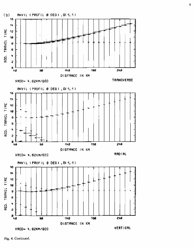
(b) ANVIL (PROFIL 0 DEG) , S ( I , l ) 16

0 r 0 90 1r0 1.90

DISTANCE I N KH

VRED- 4.62KH/SEC

2r 8

TRANSVERSE

ANVIL (PROFIL 0 DEG) , S ( 1 , 1 )

B re 98 1'40 190 2r 8

DISTANCE I N KH

VRED= 4.62KM/SEC RRD l RL

RNVIL (PROFIL 0 DEG) , S ( 1 . 1 )

DISTRNCE I N KH

VRED- 4.62KMISEC VERT l CAL

Fig. 4. Continued.

cal gradient of the P-wave phase velocity in the anisotropic layer (see Fig. la) the travel-time branch of the P wave refracted in this layer is the shortest when compared to the set of other profiles. The refracted P wave appears as the first arrival up to an offset of 160 krn in Fig. 4a. Owing to the strong gradient, its relative intensity with respect to the Moho reflection (PMP) is quite high. This corresponds to the field observations of refraction seismic data made in southwest Germany (Gajewski et al., 1987). The intensity of the corresponding refracted S waves is considerably lower (see Fig. 4b). This is due to the weak positive vertical gradient of the quasi-shear phase velocities in the anisotropic layer. The weak gradient also accounts for the quasi-shear waves qS11, qS21, qSlISl and qS2IS2 being seen at large epicentral distances. Because of the small differences in quasi-S phase velocities for this particular azimuth (Fig. lb, right side), practically no splitting of the qSlI and qS2I waves can be observed. The travel-time curves of the P and S waves refracted below the Moho (qPI1, qS11, qS2I) have extremely different slopes, which, under an assumption of isotropy would imply a large deviation of Poisson's ratio from the base value of 0.25. The wave which follows the first arrival (qP11) in Fig. 4a and continues to be seen at large epicentral distances is an interference wave formed by P waves twice refracted (qPI2) and reflected (qPI2P) in the anisotropic layer. The dominant branches on all components are the P and S Moho reflections (PMP, SMS). It is interesting to note the approximate position of the critical point on these branches. For Fig. 4a it is around 70 km. Although the wave reflected from the Moho propagates completely in an isotropic Earth's crust, the position of its critical point displays an azimuthal dependence which can be observed by comparison with the other profile directions (Figs. 5-7). This is caused by the dependence of the reflection coefficient from the Moho discontinuity upon the parameters of the underlying anisotropic layer.

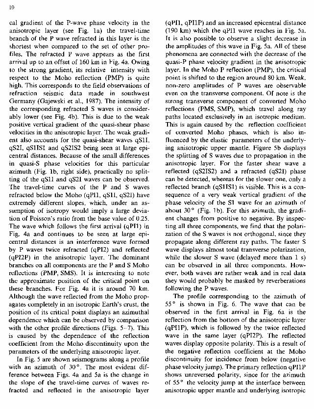
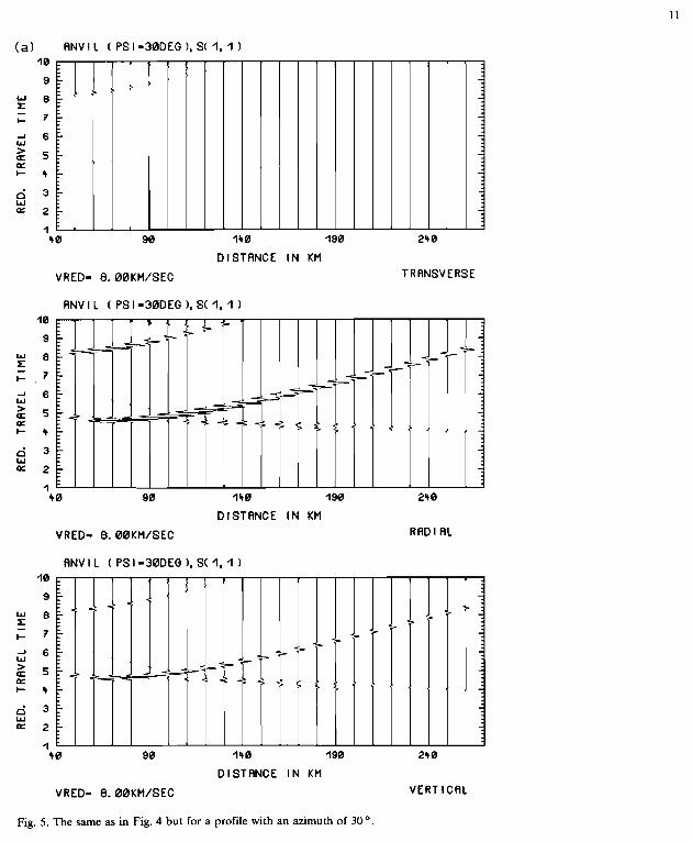
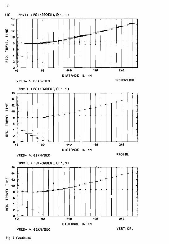
In Fig. 5 are shown seismograms along a profile with an azimuth of 30°. The most evident dif- ference between Figs. 4a and 5a is the change in the slope of the travel-time curves of waves refracted and reflected in the anisotropic layer

(qPI1, qPI1P) and an increased epicentral distance (190 krn) which the qPIl wave reaches in Fig. 5a. It is also possible to observe a slight decrease in the amplitudes of this wave in Fig. 5a. All of these phenomena are connected with the decrease of the quasi-]? phase velocity gradient in the anisotropic layer. In the Moho P reflection (PMP), the critical point is shifted to the region around 80 km. Weak, non-zero amplitudes of P waves are observable even on the transverse component. Of note is the strong transverse component of converted Moho reflections (PMS, SMP), which travel along ray paths located exclusively in an isotropic medium. This is again caused by the reflection coefficient of converted Moho phases, which is also in- fluenced by the elastic parameters of the underlying anisotropic upper mantle. Figure 5b displays the splitting of S waves due to propagation in the anisotropic layer. For the faster shear wave a reflected (qS2IS2) and a refracted (qS2I) phase can be detected, whereas for the slower one, only a reflected branch (qS1ISl) is visible. This is a consequence of a very weak vertical gradient of the phase velocity of the S1 wave for an azimuth of about 30° (Fig. lb). For ths azimuth, the gradient changes from positive to negative. By inspec- ting all three components, we find that the polarization of the S waves is not orthogonal, since they propagate along different ray paths. The faster S wave displays almost total transverse polarization, while the slower S wave (delayed more than 1 s) can be observed in all three components. How- ever, both waves are rather weak and in real data they would probably be masked by reverberations following the P waves.

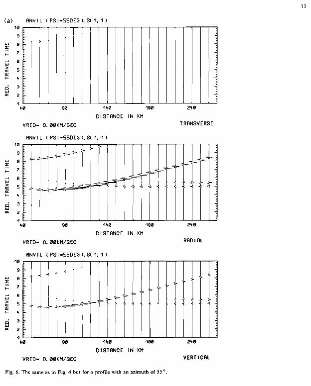
The profile corresponding to the azimuth of 55O is shown in Fig. 6. The wave that can be observed in the first arrival in Fig. 6a is the reflection from the bottom of the anisotropic layer (qPIlP), which is followed by the twice reflected wave in the same layer (qPI2P). The reflected waves display opposite polarity. This is a result of the negative reflection coefficient at the Moho discontinuity for incidence from below (negative phase velocity jump). The primary reflection qPIlP shows unreversed polarity, since for the azimuth of 55O the velocity jump at the interface between anisotropic upper mantle and underlying isotropic

(a) ANVI L ( PSI -30DEG 1, S( 1.1 1 I 0

9

w e x - I- 7

> a 5 a t- + d 3 W = 2

1 + 0 90 140 190 24 0

DISTANCE I N KM


ANVIL ( P S I - 3 0 D E G ) , S ( l . l 1

40 90 140 190 24 0

DISTANCE I N KM

VRED- 8.00KM/SEC RAD l AL

ANVIL (PSI-30DEO).S(1.1 40

9

w e f I - ?

6 W

h 5 & I- + d 3 W = 2

1 $0 90 I40 190 2+0

DISTANCE I N KM

VRED- 8.00KM/SEC VERT ICRL

Fig. 5. The same as in Fig. 4 but for a profile with an azimuth of 30 ".

0 40 90 140 190

,DISTANCE I N KM

VRED- 4.62KM/SEC

240

TRANSVERSE

ANVIL ( PSI-30DEG 1, S( 1. I )

0 +0 90 1+0 190 240

DISTANCE I N KM

VRED= +.62KM/SEC RRD l RL

RNVIL ( P S I = 3 0 D E G ) , S ( l , I ) 16

14

g 12 - t- 10 -1 W > a E d W = 2

0 40 90 140 190 24 0

DISTANCE I N KM


Fig. 5. Continued.

(a) ANV I L ( PSI -55DEG 1. S( 1, I

DISTANCE I N KM


RNV I L t PSI -55DEG ). S( 1, I 10

9

d 3 W = 2

1 + 0 90 1+0 190 240

DISTANCE I N KM

VRED- 8.00KM/SEC RAD l AL

ANV I L t PSI -55DEG 1, S( 1, I 40

I +0 90 I'i0 I@@ 240

DISTANCE I N KU

VRED- B.OOKM/SEC VERT l CAL

Fig. 6. The same as in Fig. 4 but for a profile with an azimuth of 55 O

( b) RNV I L ( PSI =55DEG ). S( 1,l 4 6

0 +0 90 190 190

DlSTRNCE I N KM

VRED- 4.62KM/SEC

29 0

TRRNSVERSE

ANVIL ( P S I - S S D E G ) , S ( I , l )

ANVIL (PSI=SSDEG) ,S( l , I )

- 40 9fi 140 190 24 0

DISTANCE I N KM

VRED- 4. 62KM/SEC VERT l CAL

Fig. 6. Continued.

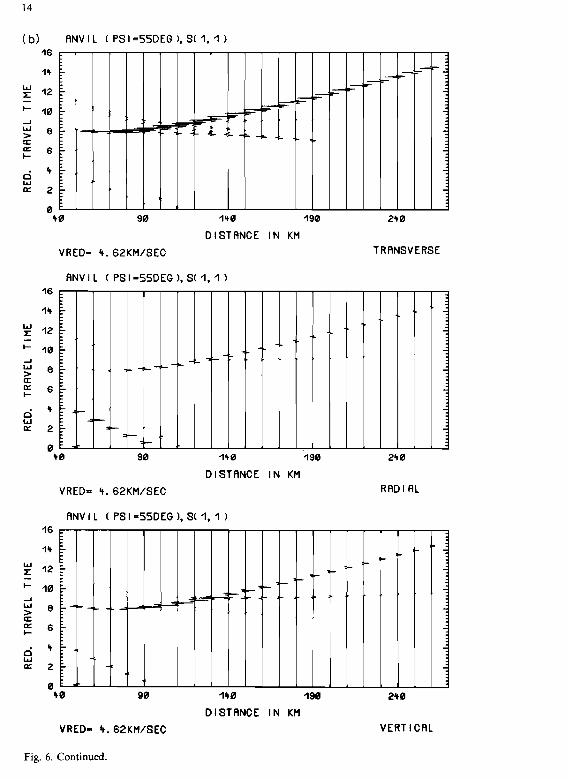
layer is positive in contrast to the previous profiles where this jump was negative (Fig. la). The refracted wave qPIl is so weak that is is not observable. This is a consequence of the very weak gradient of its phase velocity. The transverse components of the qPIlP, PMS and SMP phases, although observable, are again very weak. The prominent feature of Fig. 6b is the strong arrival on the transverse component corresponding to an S wave refracted in the anisotropic layer (qS2I). The strong amplitudes are caused by the largest vertical gradient of the phase velocity of the S2 wave existing for this particular azimuth (Fig. Ib). The reflected branch (qS21S2) of this phase can also be observed on the transverse component in the traces between epicentral distances of 100-130 km. This is closely followed by a surprisingly strong quasi-shear wave conversion (qSlIS2) from the bottom of the anisotropic layer. It has an intensity as strong as the unconverted reflection qS2IS2. The converted arrivals can be observed between epicentral distances of 100 and 150 km, where this phase terminates. The slower refracted S wave (qS1I) is missing due to the negative gradient of its phase velocity. The reflected branch observed on all three components up to the end of the profile and preceding the Moho reflection SMS corresponds to the reflection of the slower S wave from the bottom of the anisotropic layer (qSlIS1). In this example, refracted shear-wave amplitudes reach very high intensities, which on some traces are of a magnitude comparable to the amplitudes of the dominant Moho reflection (SMS).

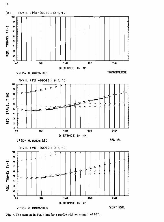
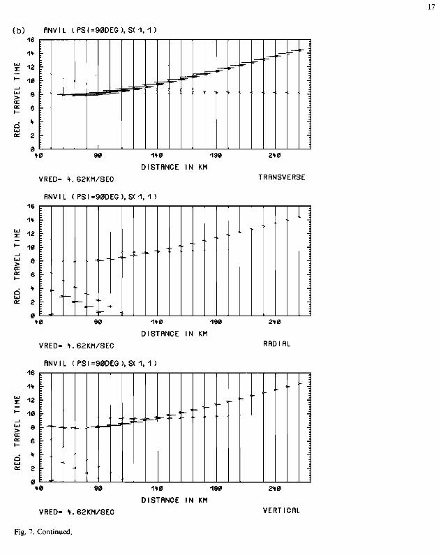
The profile corresponding to the azimuth of 90 O, shown in Fig. 7, is again in a direction that corresponds to a near symmetry plane. Therefore, no P waves are observed on the transverse component. The critical-point position on the Moho P reflection (PMP) reaches maximum range at about 90 km in this case. The amplitudes of the reflections are generally smaller than on the previous profiles due to the descrease of the velocity contrast across the Moho. In Fig. 7b, an obvious splitting of reflected S waves (qSlIS1, qS2IS2) can be seen. The faster phase has mainly a transverse component, while the slower one has components in both radial and vertical directions (in this case

the polarization of S waves is close to SV and SH polarization). All other features of Fig. 7 are sirni- lar to the features discussed for the previous profile (see the description of Fig. 6).

3.2. Fan synthetic sections

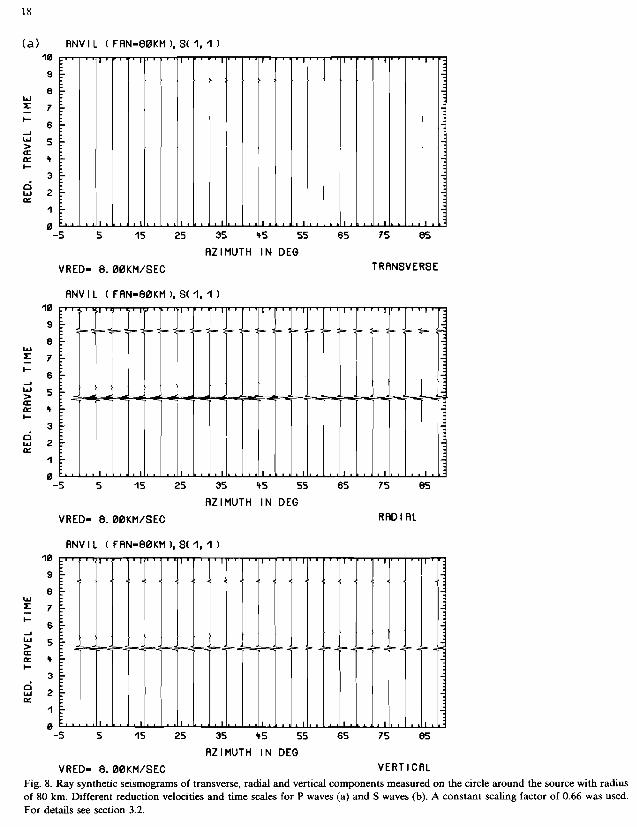
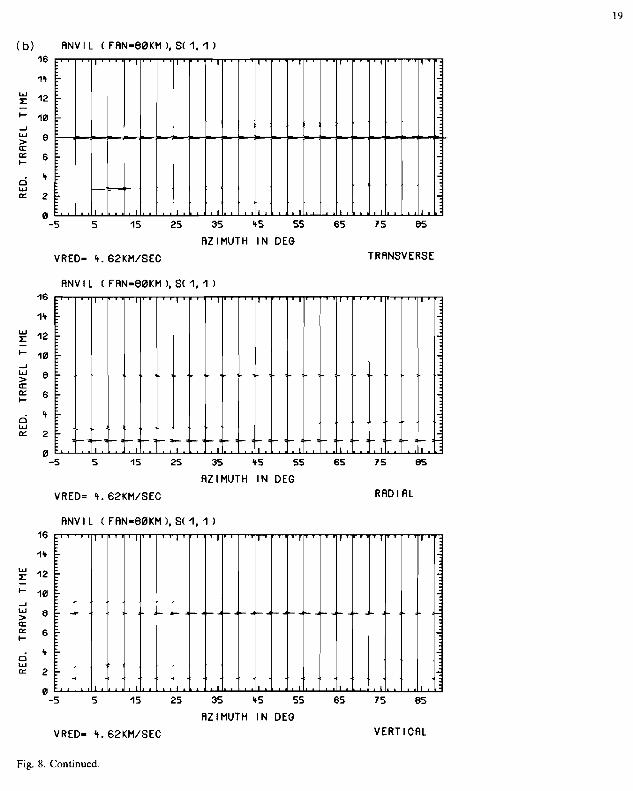
Synthetic sections recorded on a quarter of two concentric circles around the source, with radii of 80 and 150 km are shown in Figs. 8 and 9. In Fig. 8 amplitudes are reduced by a factor of 0.66 so as to reveal better the phase changes of the unconverted Moho reflections near the critical epicentral distances (about 80 km).

The most prominent waves in Fig. 8 are the Moho reflections, whose arrival times are ap- proximately 4.4 s for P waves and 8 s for S waves. Since these propagate in the isotropic Earth's crust, their travel-time curves are horizontal lines (all seismograms are recorded at a constant offset). Closer inspection of the form of individual signals reveals, however, that their shape and amplitude change with azimuth. This is another display of the critical-point shift phenomena, discussed in the preceding sections. The waves following the Moho reflection are the reflections from the bottom of the anisotropic layer. These waves already display azimuthal dependence of travel times. The strong arrival with azimuthally dependent intensity, at 8.5 s in Fig. 8a is an interference of the reflected converted waves from the crust-mantle boundary (PMS, SMP). These arrivals can be detected even on the transverse component, which again is an exhibition of the influence of the underlying anisotropic upper mantle on the crustal phases propagating in an isotropic medium. For azimuths close to symmetry planes (close to O 0 and 90 O), this amval is not seen in the transverse component. Note, that neither P nor S waves refracted in the anisotropic layer are observed at this epicentral distance. The weak reverberations close to 9.5 s in Fig. 8b, just following the SMS reflection, are caused by the quasi-shear waves qSlIS1, qS2IS2, qSlIS2 and qS2IS1. The arrivals near 2 s in Fig. 8b are converted waves, the fastest corresponding to the PMS, SMP reflections discussed above, while the slower events are converted reflections from the bottom of the

(a) ANV I L ( PSI -90DEG I, S( 1.1

40 90 140 190 2'1 0

DISTANCE I N KM


ANVIL (PSI -90DEG) ,S(1 .1 )

+0 90 140 190 24 0

DISTANCE I N KM

VRED- 8.00KM/SEC RAD I AL

ANVIL ( P S I - 9 0 D E 8 ) , S ( I , l 10

9

w e x - I- 7

6 W > a 5 a + 4

d 3 W = 2

1 50 90 140 190 250

DISTANCE I N KM


Fig. 7. The same as in Fig. 4 but for a profile with an azimuth of 90°.

RED.

TR

AVE

L T

IME

RE

D.

TRA

VEL

TIM

E

RED.

TR

AVE

L T

IME

,-.

u -

(a) RNVIL (FRN-80KM).S(1,11

0 -5 5 15 25 35 45 55 65 75 85

AZIMUTH I N DEG

VRED- 8.00KM/SEC TRRNSVERSE

RNV I L ( FAN-80KM ), S( 1 , l 1 I0

9

B -5 5 15 25 35 45 55 65 75 85

RZIMUTH I N DEG

VRED- 8.00KM/SEC RRD l RL

RNV I L ( FRN-80KM 1, S( 1.1 1 10

9

1

0 -5 5 15 25 35 45 55 65 75 85

AZIMUTH I N DEG

VRED- 8.00KM/SEC VERT l CRL Fig. 8. Ray synthetic seismograms of transverse, radial and vertical components measured on the circle around the source with radius of 80 km. Different reduction velocities and time scales for P waves (a) and S waves (b). A constant scaling factor of 0.66 was used. For details see section 3.2.

l't

0 -5 5 15 25 35 45 55 65 75 85

RZIMUTH I N DEG


RNV I L ( FRN-BOKM 1, S( 1.1

0 -5 5 15 25 35 45 55 65 75 85

RZIMUTH I N DEG

VRED= C. 62KM/SEC RRD l AL

RNV I L ( FRN-80KM 1, S( 1, I

RZIMUTH I N DEG

VRED- 4. 62KM/SEC VERT l CAL

Fig. 8. Continued

( a ) ANV I L ( FAN-IS0KM 1, S( 1.1

AZIMUTH I N DEQ


ANVIL ( FAN-ISBKM ), Sf 1. I ) I 0

I

0 -5 5 15 25 35 45 55

AZIMUTH I N DEG

VRED- 8.00KM/SEC

65 75 85

RAD l AL

RNVI L ( FAN-ISBKM 1. S( 1.1 ) 10

1

0 -5 5 15 25 35 45 55

AZIMUTH I N DEG

VRED- 8. 00KM/SEC

65 I 5 85

VERT l CAL

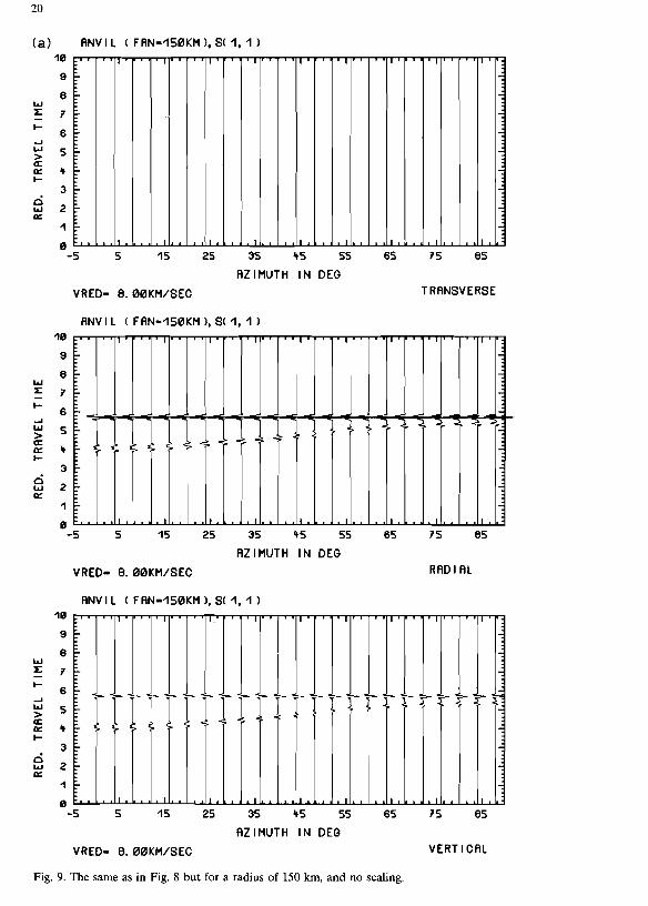
Fig. 9. The same as in Fig. 8 but for a radius of 150 km, and no scaling.

( b ) ANVI L ( FAN=150KM 1, S( 1, I )

AZIMUTH I N DEG

VRED- 4.62KM/SEC TRRNSVERSE

RNVI L ( FRN-I50KM 1. S( 1. I )

AZIMUTH I N DEG

VRED= 4.62KM/SEC RRD l AL

RNV I L ( FAN-I50KM ). S( 1, I

AZIMUTH I N DEG

VRED- +.62KM/SEC VERT l CAL

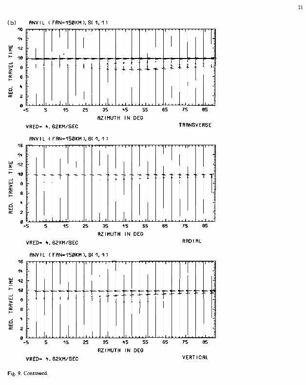
Fig. 9. Continued.

anisotropic layer (qPIS1, qSlIP and qPIS2, qSZIP), which differ only slightly in time.

Figure 9 shows a synthetic section recorded on a fan with a radius of 150 km. For the Moho reflections (PMP - 5.5 s, SMS - 9.6 s) t h s is a supercritical distance, therefore the amplitudes as well as the wave forms of Moho reflections are practically azimuthally independent. At this range, the waves refracted in the subcrustal anisotropic layer can be observed. They display strong azimuthal dependence both in arrival times and amplitude. In Fig. 9b the refracted waves for some azimuths disappear completely due to the negative vertical gradient of the corresponding phase velocities (Fig. lb). The refracted waves are followed immediately by reflections from the bottom of the anisotropic layer. As was stated previously, the S wave with a prevailing transverse component propagates faster than the other S-wave type, which can be observed on all three displacement components. The amplitudes of the split shear waves are rather large, especially for azimuths close to 50 ".

4. Discussion of numerical results and observed data

The numerical results are in a good qualitative agreement with P-wave observations. Extremely high apparent P-wave velocities as well as PMP/qPIl amplitude ratios close to unity can be observed in the refraction seismic data from southwest Germany (Gajewski et al., 1987). Both of these phenomena are in a good agreement with the numerical results. The observed data also show, as do the numerical results, azimuthal dependence of travel times and amplitudes of P waves.

In the case of shear waves, numerical results show that for some azimuths, relatively strong split shear-wave arrivals should be expected. In real data, however, to this point in time no refracted upper-mantle shear wave has been observed. On the other hand, crustal shear waves, specifically reflections from the crust-mantle boundary (SMS), are recorded on all components, similar to the computed SMS onsets. Even in the

case of extremely strong refracted upper-mantle P waves, no shear-wave arrivals were recorded. This may indicate either anisotropy of a different type than that considered in the ANVIL model, or a strong deviation of Poisson's ratio from the assumed value of 0.25 in the isotropic upper mantle of southwest Germany. Another possible explana- tion could be a lower value of Q for shear waves in the upper mantle. The ANVIL model cannot explain the absence of shear-wave observations, as it produces shear arrivals from the upper mantle which are too strong. This remains true even for a more realistic type of source than that used in the present study. This follows from the quahtatively good agreement between observed and computed shear-wave Moho reflections. The range of initial angles of upper-mantle refracted shear waves is practically the same as that of the shear-wave reflections from the crust-mantle boundary. Since clear SMS reflections are observed in the computed and recorded data for all components, the missing upper mantle shear-wave data must be due to the physical properties of the upper mantle and not the source properties. It should be mentioned, that when Fuchs (1983) suggested the ANVIL model on the basis of refraction seismic P-wave data from southwest Germany, no high quality shear-wave observations were available. To make quantitative conclusions on an anisotropic upper mantle and the ANVIL model, we need to take into account the complicated 3-D isotropic crustal structure of southwest Germany (Gajewslu et a]., 1987) and the shape of the crust-mantle boundary as it descends beneath the Alps. Com- putations for such complicated 3-D structures can be performed with the program package described here. It will be, however, a rather complicated task to fit observed travel times and amplitudes of both P and S waves, dealing with modelling techniques based on varying both the anisotropy and inhomogeneity of a 3-D structure. Experience in treat- ing data from anisotropic structures and probably new observation techniques, different from those presently used, are required. Numerical experi- ments are expected to play an important role in this process.

5. Conclusions Acknowledgements

A procedure for the evaluation of ray synthetic seismograms in 3-D laterally varying layered anisotropic structures was programmed, and first examples of its application presented. For test purposes, the ANVIL model, a model of the continental subcrustal lithosphere in southern Germany was used. Although the parameters of the model change only with depth, due to its anisotropic properties, the model requires a 3-D treatment.

The main conclusions that follow from this study are related for the most part to the P waves propagating in an anisotropic structure. The rea- sons for t h s are the following. First, the model used for the study was derived from the P-wave observations. Second, the S-wave source considered in the study was to some extent artificial. Finally, the procedure employed may give arnpli- tudes and polarizations of S waves whch are not sufficiently accurate if the phase velocities of the two quasi-S waves propagating in the anisotropic layer are close to one another. Nonetheless, even with the mentioned limitations, some conclusions for the S waves may be drawn from this study.

The most prominent features observed were the azimuthal dependence of the maximum range and amplitude of waves refracted in the anisotropic layer, the azimuthally dependent shift of the critical point of the Moho reflections, and the refracted and reflected shear-wave splitting. It is also worth mentioning, that the apparent velocities of P and S waves in the synthctic data would lead to extreme deviations from a Poisson's ratio of 0.25, if isotropy were assumed for the interpretation of such kind of data.

The study undertaken shows that even in simple models like the one presented in this paper, which displays a relatively high symmetry of elastic properties (orthorhombic symmetry) and a low measure of inhomogeneity (vertical inhomogeneity), 3-D modelling is a necessity. It also confirms the well known fact that without three-component recording, there is little chance to observe seis~nic anisotropy. Finally, this study seems to indicate that to obtain observable effects of seismic anisotropy on shear waves, controlled shear-wave source seismology should be used.

The authors thank Professor K. Fuchs for fruit- ful discussions and Pat Daley for a critical review of the paper.

References

Babich, V.M., 1961. Ray method for the computation of the intensity of wave fronts in elastic inhomogeneous anisotropic medium. In: Problems of the Dynamic Theory of Propagation of Seismic Waves, 5. Leningrad, University Press, Leningrad, pp. 36-46 (in Russian).

Cerveng, V., 1972. Seismic rays and ray intensities in inhomogeneous anisotropic media. Geophys. J.R. Astron. Soc.. 29: 1-13.

Cerveng, V. and Firbas, P., 1984. Numerical modelling and inversion of travel-time fields of seismic body waves in inhomogeneous anisotropic media. Geophys. J.R. Astron. Soc., 76: 41-51.

Cerveng, V. and PSenEik, I., 1972. Rays and travel-time curves in inhomogeneous anisotropic media. J. Geophys., 38: 565-578.

Cerveng, V. and PSenEik. I., 1984. SEIS83 - Numerical model- ing of seismic wave fields in 2-D laterally varying layered structures by the ray method. In: E.R. Engdahl (Editor), Documentation of Earthquake Algorithms. World Data Center (A) for Solid Earth Geophysicists, Boulder, Col- orado, Report SE-35, pp. 36-40.

Cervenq, V., Molotkov, I.A. and PSenEik, I., 1977. Ray Method in Seismology. Charles University Press, Prague, 210 pp.

Crampin, S., 1981. A review of wave motion in anisotropic and cracked elastic media. Wave Motion, 3: 343-391.

Fedorov, F.I., 1968. Theory of Elastic Waves in Crystals. Plenum Press, NY. 375 pp.

Fuchs, K., 1983. Recently formed elastic anisotropy and petro- logical models for the continental subcrustal lithosphere in southern Germany. Phys. Earth Planet. Inter., 31: 93-118.

Gajewski, D. and PSenEik, I., 1987. Computation of high- frequency seismic wave fields in 3-D laterally inhomogeneous anisotropic media. Geophys. J.R. Astron. Soc., 91: 383-411.

Gajewski, D., Holbrook, W.S. and Prodehl, C., 1987. A three- dimensional crustal model of southwest Germany derived from refraction seismic data. Tectonophysics, 42: 49-70.

Gruenewald, M., 1986. Body wave seismograms for anisotropic gradient zones with the reflectivity method. Terra cognita, 6: 307.

Hanyga, A,, 1986. Gaussian beams in anisotropic elastic media. Geophys. J.R. Astron. Soc., 85: 473-503.

Kravtsov, Yu. A. and Orlov, Yu. I., 1980. Geometrical Optics of Inhomogeneous Media. Nauka, Moscow, 304 pp. (in Russian).

Mikhadenko, B.G., 1985. Numerical experiment in seismic investigations. J. Geophys., 58: 101-124.

Documents

Ray synthetic seismograms for a 3-D anisotropic …seis.karlov.mff.cuni.cz/papers.bin/a88ip1.pdf · each elementary wave and each receiver position 3. Ray synthetic seismograms for