Machine Learning

Azure Machine Learning Lab

What is Azure Machine Learning?The Problem DomainFirst Time SetupThe DataData Pre-ProcessingTraining the ModelOptimising ClassifiersCreating a Scoring ExperimentPublish as a Web ServiceTesting the Web ServicePublish to the GalleryConclusion

Contents

This lab will introduce you to machine learning capabilities available in Microsoft Azure. Microsoft Azure Machine Learning (Azure ML) allows you to create basic designs and complete experimentation and evaluation tasks. In this lab, we will cover Azure ML Studio, a fully managed machine learning platform that allows you to perform predictive analytics. Azure ML Studio is a user facing service that empowers both data scientists and domain specialists to build end-to-end solutions and significantly reduce the complexity of building predictive models. It provides an interactive and easy to use web-based interface with drag-and-drop authoring and a catalogue of modules that provide functionality for an end-to-end workflow.In some scenarios a data scientist may not understand the domain data as thoroughly as a domain expert does. Microsoft Azure Machine Learning has made it possible for the people who know the most about the data to produce predictive analytics for that data.

What is Azure Machine Learning?

During this lab, you will create and publish a model that predicts if a flight will be delayed depending on a range of flight details and weather data. The two datasets used are flight delay data and weather data. These sets consist of records for flights and the weather at each airport on an hourly basis. The columns of the flight delay dataset hold information such as the date and time of a flight, the carrier, origin and destination ID’s as well as delay time information.The columns of the weather dataset hold information such as the Airport ID, date and time and various weather measures such as visibility and temperatures.The model you will create is a form of supervised learning; we will use historical flight and weather data to predict if a future flight is delayed. This model will use a binary classification technique, is the flight delayed or not, and produce a web service you can query with new flights

The Problem Domain

Microsoft Azure Machine Learning offers a free-tier service and a standard tier for which you need an Azure subscription. In order to access the free workspace, go to https://studio.azureml.net/ , sign in with a Microsoft account (@hotmail.com, @outlook.com etc.) and a free workspace is automatically created for you.If you wish to use an Azure subscription to create a paid workspace, you will need an Azure subscription to complete the lab. You can sign up for a free Azure one month trial; using your Microsoft account; where you get £125 to try out all the services in Azure. Sign up to Azure for one month free trial here: http://azure.microsoft.com/en-gb/pricing/free-trial/ If you don’t have a Microsoft account, create one here: https://signup.live.com/signup.aspxOnce you have an Azure subscription you can go to http://www.azure.microsoft.com and choose ‘My Account’ at the top of the page then choose the ‘Management Portal’ where it will ask you to sign in with your Microsoft account.Once into the management portal scroll down the toolbar on the left side of the screen and find the Machine Learning Icon. To create a new workspace click on the ‘New’, ‘Data Services’, ‘Machine Learning’ and ‘Quick Create’.

First Time Setup

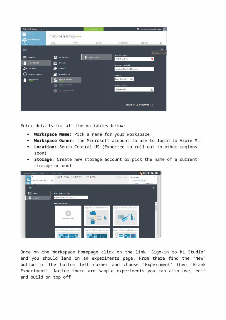
Enter details for all the variables below: Workspace Name: Pick a name for your workspace Workspace Owner: the Microsoft account to use to login to Azure ML. Location: South Central US (Expected to roll out to other regions soon) Storage: Create new storage account or pick the name of a current storage

account.

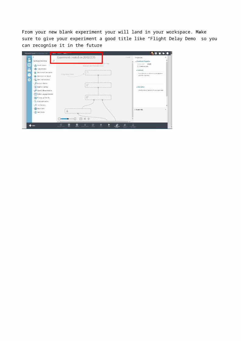
Once on the Workspace homepage click on the link ‘Sign-in to ML Studio’ and you should land on an experiments page. From there find the ‘New’ button in the bottom left corner and choose ‘Experiment’ then ‘Blank Experiment’. Notice there are sample experiments you can also use, edit and build on top off.From your new blank experiment your will land in your workspace. Make sure to give your experiment a good title like “Flight Delay Demo” so you can recognise it in the future

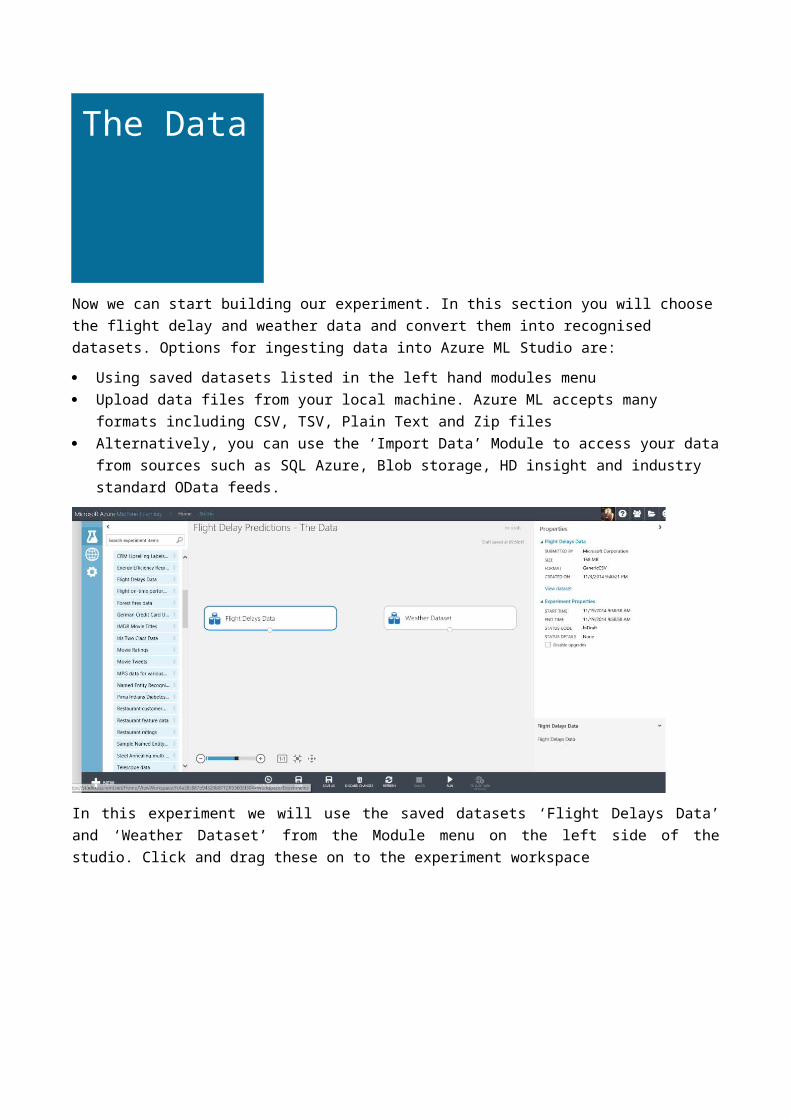
Now we can start building our experiment. In this section you will choose the flight delay and weather data and convert them into recognised datasets. Options for ingesting data into Azure ML Studio are: Using saved datasets listed in the left hand modules menu Upload data files from your local machine. Azure ML accepts many formats including

CSV, TSV, Plain Text and Zip files Alternatively, you can use the ‘Import Data’ Module to access your data from

sources such as SQL Azure, Blob storage, HD insight and industry standard OData feeds.

In this experiment we will use the saved datasets ‘Flight Delays Data’ and ‘Weather Dataset’ from the Module menu on the left side of the studio. Click and drag these on to the experiment workspace

The Data

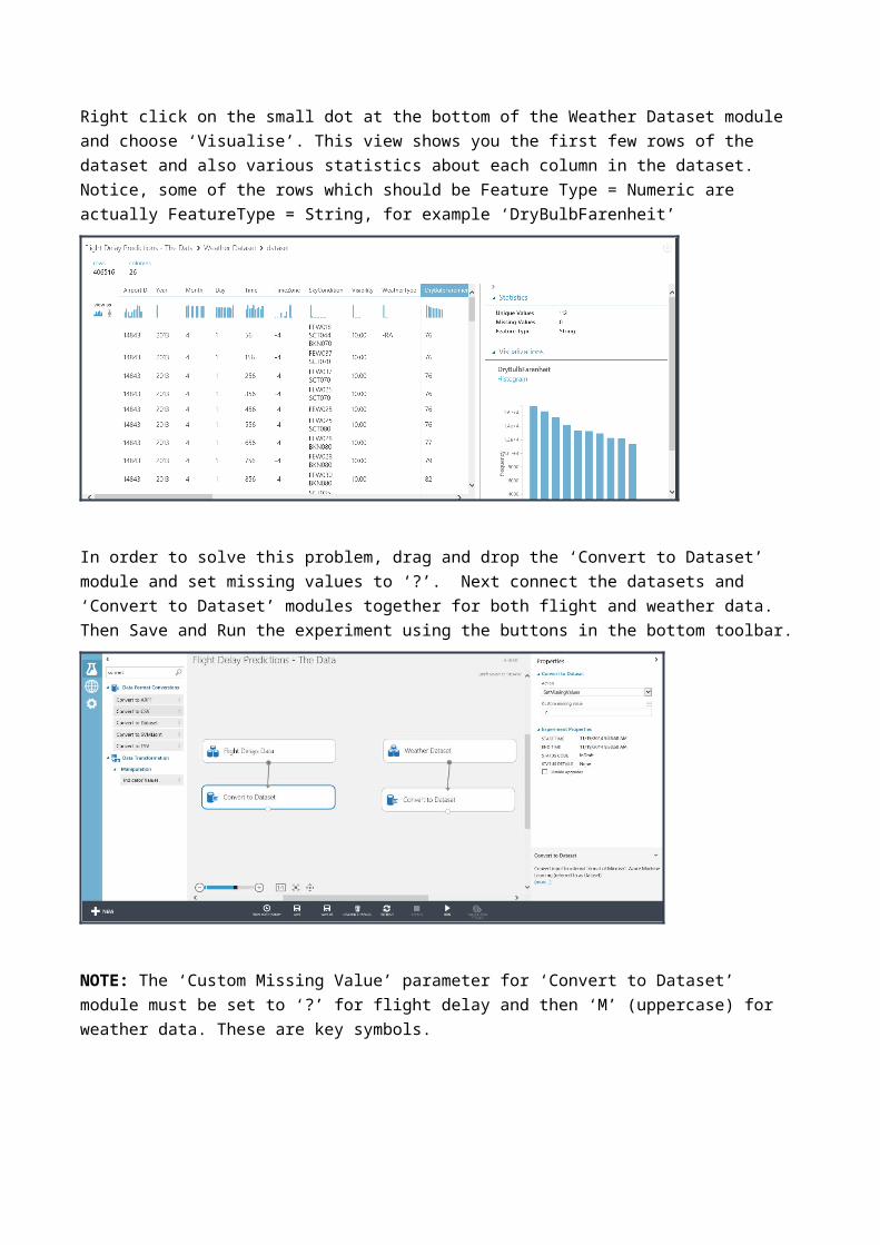
Right click on the small dot at the bottom of the Weather Dataset module and choose ‘Visualise’. This view shows you the first few rows of the dataset and also various statistics about each column in the dataset. Notice, some of the rows which should be Feature Type = Numeric are actually FeatureType = String, for example ‘DryBulbFarenheit’

In order to solve this problem, drag and drop the ‘Convert to Dataset’ module and set missing values to ‘?’. Next connect the datasets and ‘Convert to Dataset’ modules together for both flight and weather data. Then Save and Run the experiment using the buttons in the bottom toolbar.

NOTE: The ‘Custom Missing Value’ parameter for ‘Convert to Dataset’ module must be set to ‘?’ for flight delay and then ‘M’ (uppercase) for weather data. These are key symbols.

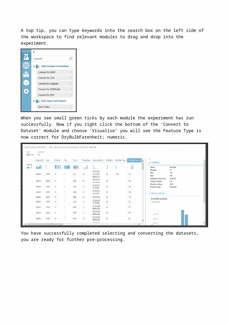
A top tip, you can type keywords into the search box on the left side of the workspace to find relevant modules to drag and drop into the experiment.

When you see small green ticks by each module the experiment has run successfully. Now if you right click the bottom of the ‘Convert to Dataset’ module and choose ‘Visualise’ you will see the Feature Type is now correct for DryBulbFarenheit; numeric.

You have successfully completed selecting and converting the datasets, you are ready for further pre-processing.

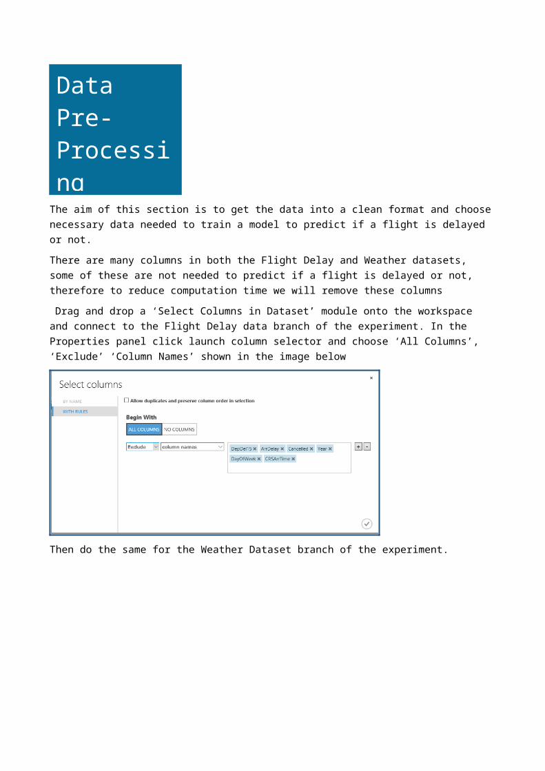
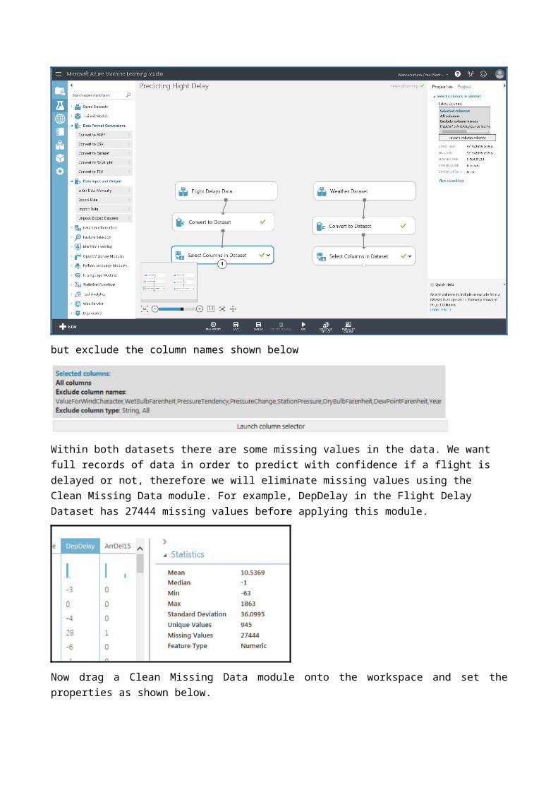
The aim of this section is to get the data into a clean format and choose necessary data needed to train a model to predict if a flight is delayed or not. There are many columns in both the Flight Delay and Weather datasets, some of these are not needed to predict if a flight is delayed or not, therefore to reduce computation time we will remove these columns Drag and drop a ‘Select Columns in Dataset’ module onto the workspace and connect to the Flight Delay data branch of the experiment. In the Properties panel click launch column selector and choose ‘All Columns’, ‘Exclude’ ‘Column Names’ shown in the image below

Then do the same for the Weather Dataset branch of the experiment.

Data Pre-Processing

but exclude the column names shown below

Within both datasets there are some missing values in the data. We want full records of data in order to predict with confidence if a flight is delayed or not, therefore we will eliminate missing values using the Clean Missing Data module. For example, DepDelay in the Flight Delay Dataset has 27444 missing values before applying this module.

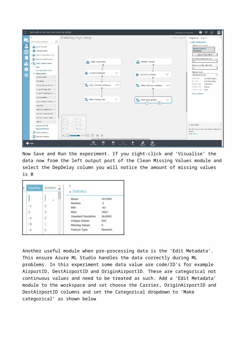
Now drag a Clean Missing Data module onto the workspace and set the properties as shown below.

Now Save and Run the experiment. If you right-click and ‘Visualise’ the data now from the left output port of the Clean Missing Values module and select the DepDelay column you will notice the amount of missing values is 0

Another useful module when pre-processing data is the ‘Edit Metadata’. This ensure Azure ML Studio handles the data correctly during ML problems. In this experiment some data value are code/ID’s for example AirportID, DestAirportID and OriginAirportID. These are categorical not continuous values and need to be treated as such. Add a ‘Edit Metadata’ module to the workspace and set choose the Carrier, OriginAirportID and DestAirportID columns and set the Categorical dropdown to ‘Make categorical’ as shown below

To predict if a flight is delayed we want use both the flight and weather data therefore we need to join the datasets. Currently we have month, day and AirportID that can join in each dataset, however we want to match on the time as well. Currently the flight time is to the nearest minute and the weather time recordings are once an hour at 56 minutes past.Now we will transform the time and round to the hour. Drag and drop the ‘Apply Math Operation’ module onto the workspace and connect to the Flight Delay Data branch. Set the Properties as shown below:

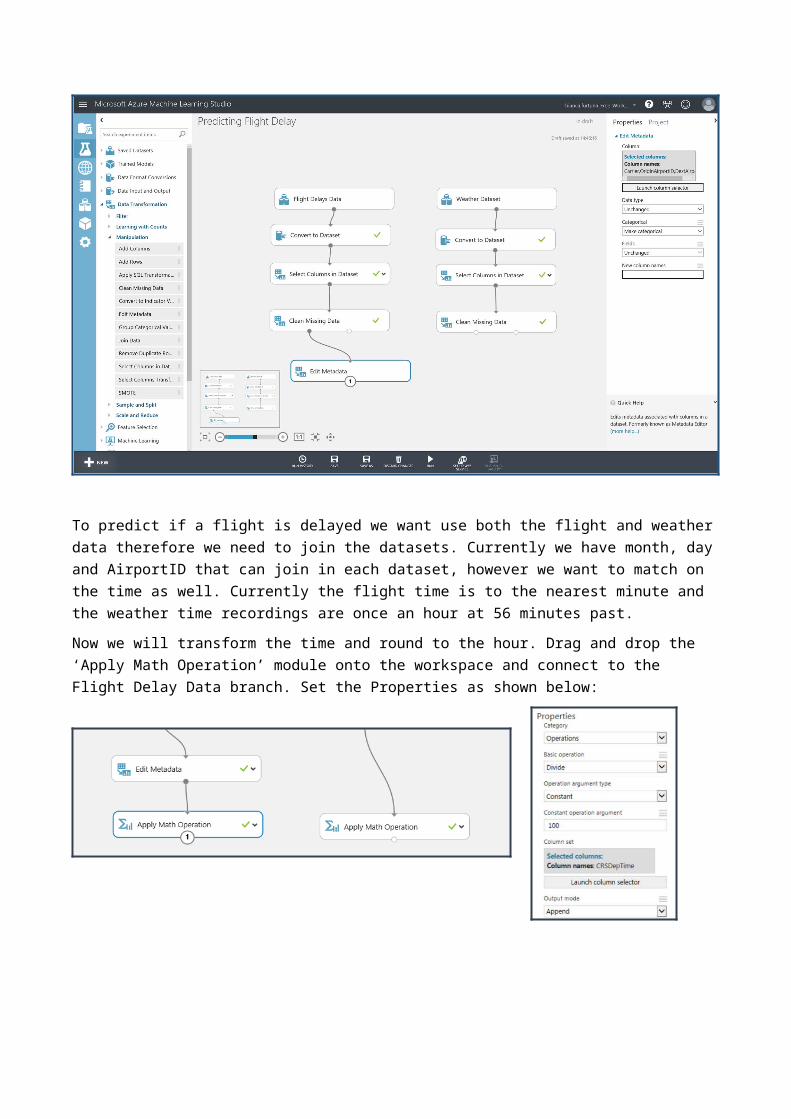
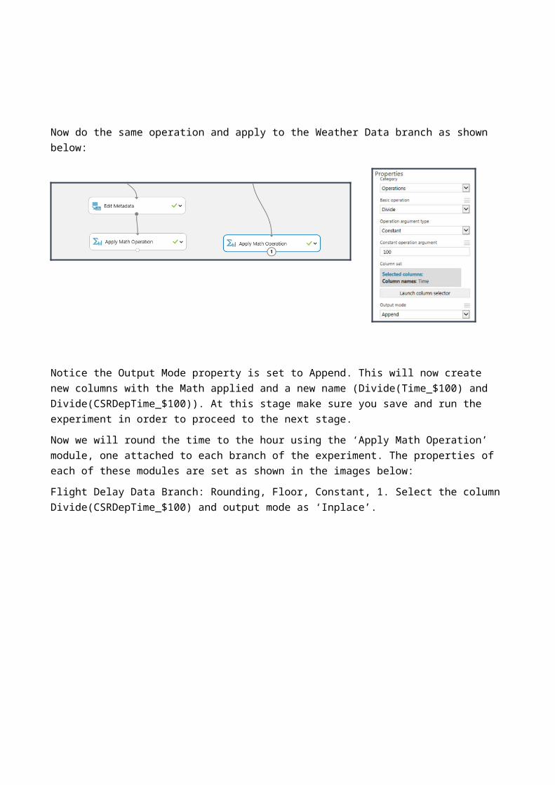
Now do the same operation and apply to the Weather Data branch as shown below:

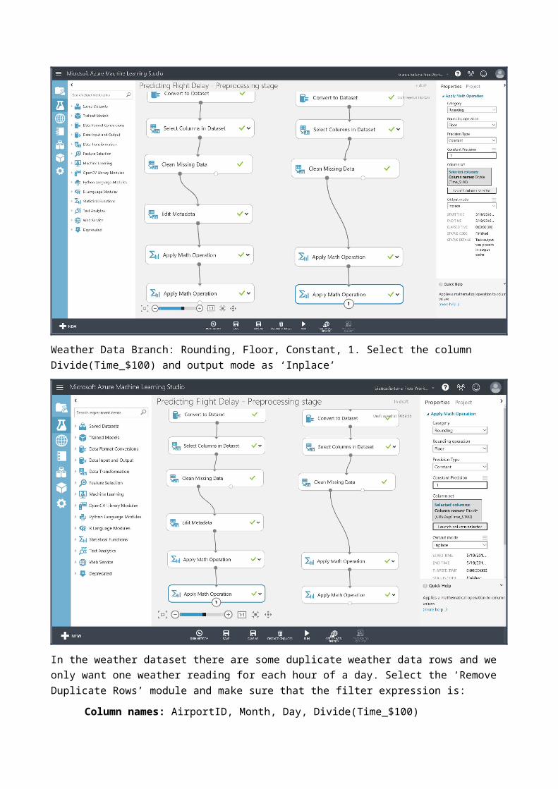
Notice the Output Mode property is set to Append. This will now create new columns with the Math applied and a new name (Divide(Time_$100) and Divide(CSRDepTime_$100)). At this stage make sure you save and run the experiment in order to proceed to the next stage. Now we will round the time to the hour using the ‘Apply Math Operation’ module, one attached to each branch of the experiment. The properties of each of these modules are set as shown in the images below:Flight Delay Data Branch: Rounding, Floor, Constant, 1. Select the column Divide(CSRDepTime_$100) and output mode as ‘Inplace’.

Weather Data Branch: Rounding, Floor, Constant, 1. Select the column Divide(Time_$100) and output mode as ‘Inplace’

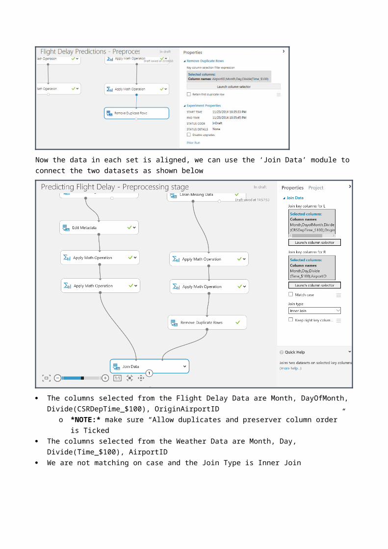
In the weather dataset there are some duplicate weather data rows and we only want one weather reading for each hour of a day. Select the ‘Remove Duplicate Rows’ module and make sure that the filter expression is:

Column names: AirportID, Month, Day, Divide(Time_$100)

Now the data in each set is aligned, we can use the ‘Join Data’ module to connect the two datasets as shown below

The columns selected from the Flight Delay Data are Month, DayOfMonth, Divide(CSRDepTime_$100), OriginAirportID

o *NOTE:* make sure “Allow duplicates and preserver column order” is Ticked The columns selected from the Weather Data are Month, Day, Divide(Time_$100),

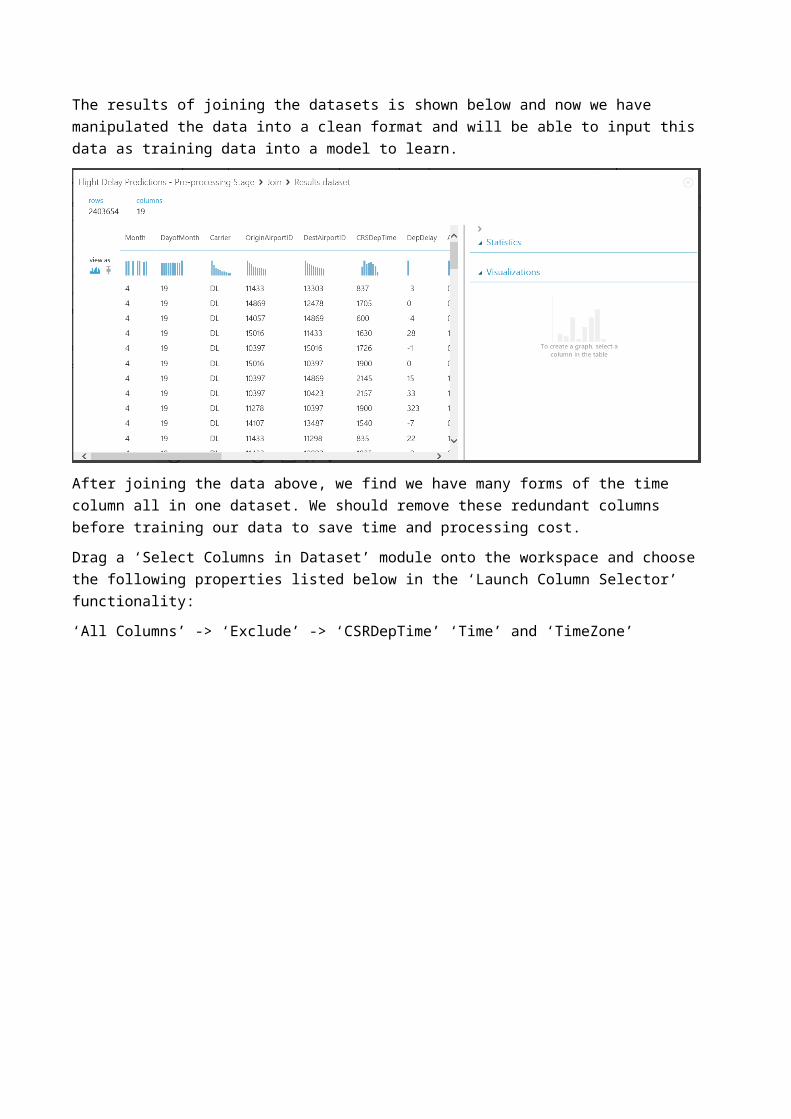
AirportID We are not matching on case and the Join Type is Inner JoinThe results of joining the datasets is shown below and now we have manipulated the data into a clean format and will be able to input this data as training data into a model to learn.

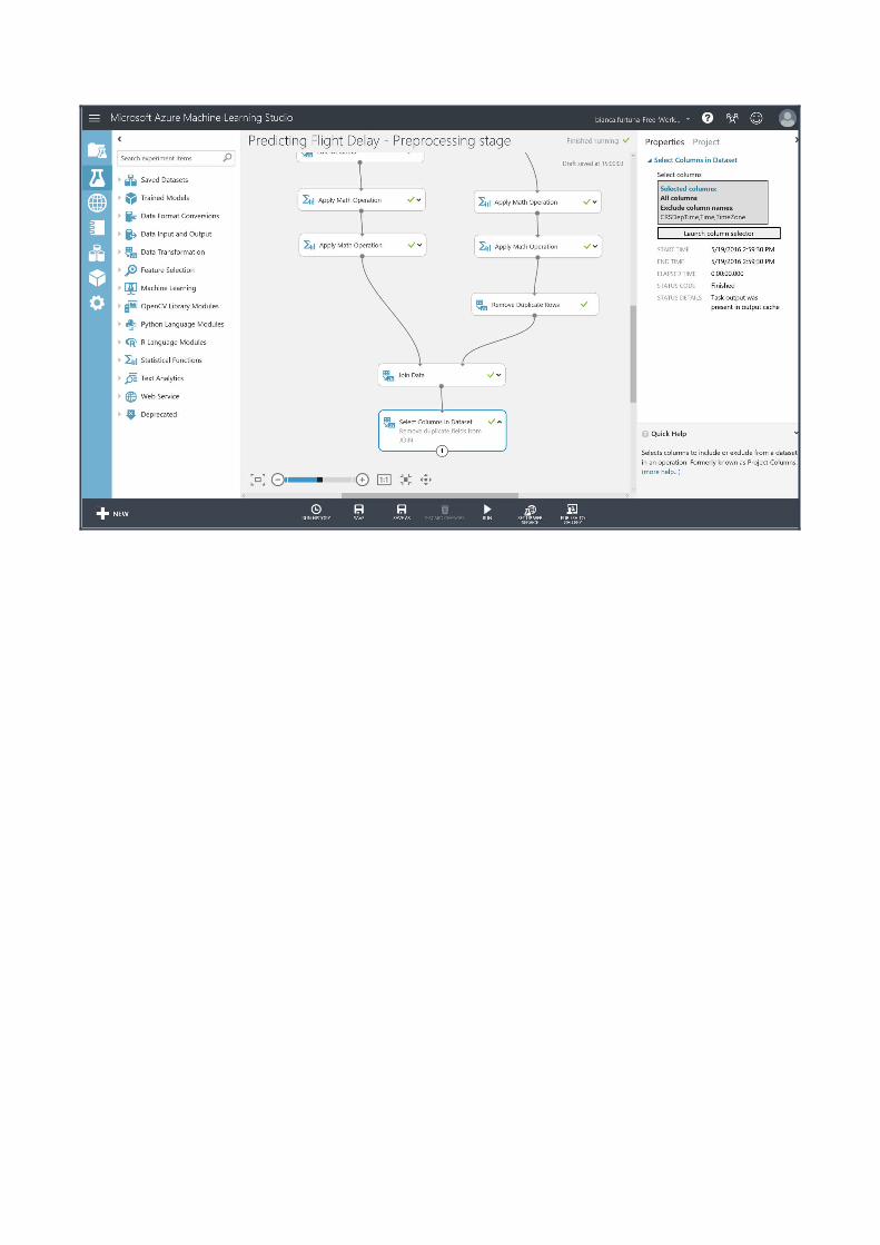
After joining the data above, we find we have many forms of the time column all in one dataset. We should remove these redundant columns before training our data to save time and processing cost.Drag a ‘Select Columns in Dataset’ module onto the workspace and choose the following properties listed below in the ‘Launch Column Selector’ functionality:‘All Columns’ -> ‘Exclude’ -> ‘CSRDepTime’ ‘Time’ and ‘TimeZone’

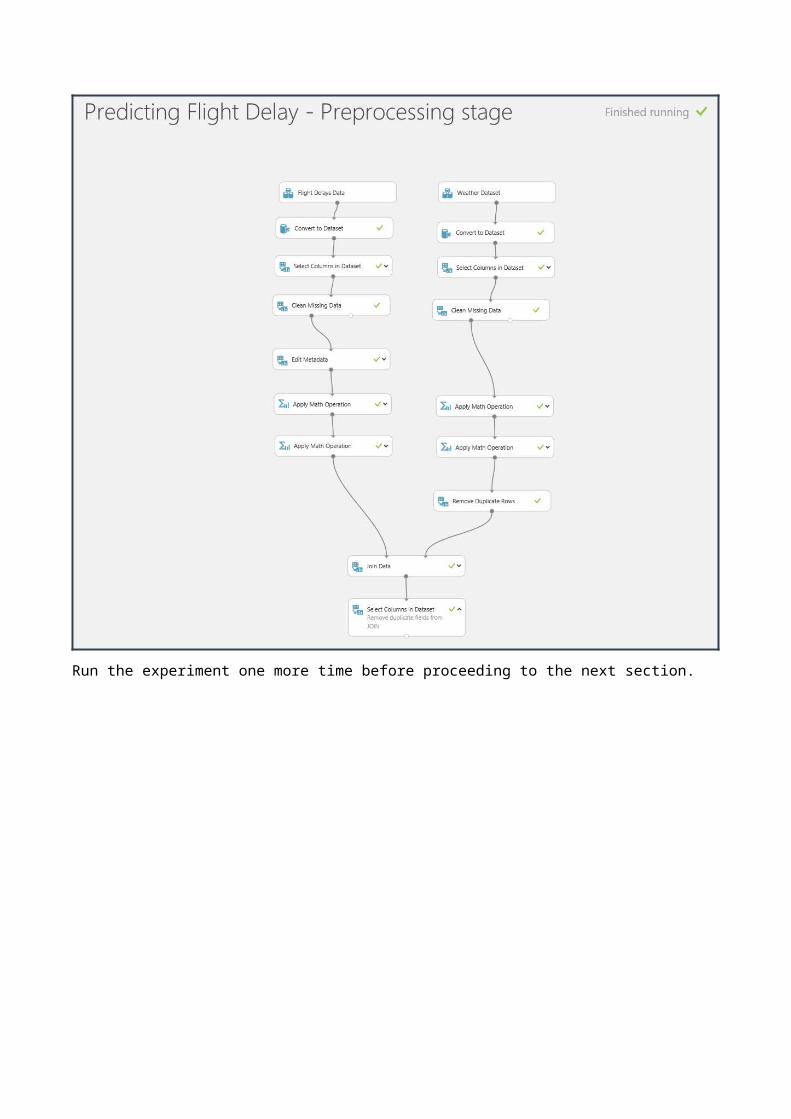
Run the experiment one more time before proceeding to the next section.

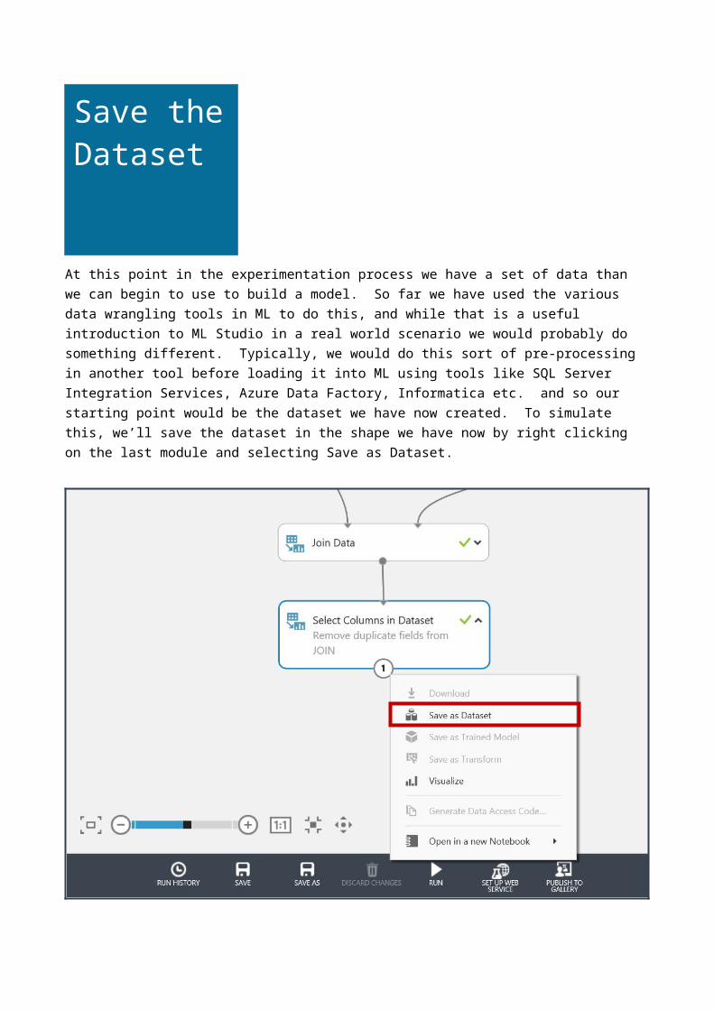
At this point in the experimentation process we have a set of data than we can begin to use to build a model. So far we have used the various data wrangling tools in ML to do this, and while that is a useful introduction to ML Studio in a real world scenario we would probably do something different. Typically, we would do this sort of pre-processing in another tool before loading it into ML using tools like SQL Server Integration Services, Azure Data Factory, Informatica etc. and so our starting point would be the dataset we have now created. To simulate this, we’ll save the dataset in the shape we have now by right clicking on the last module and selecting Save as Dataset.

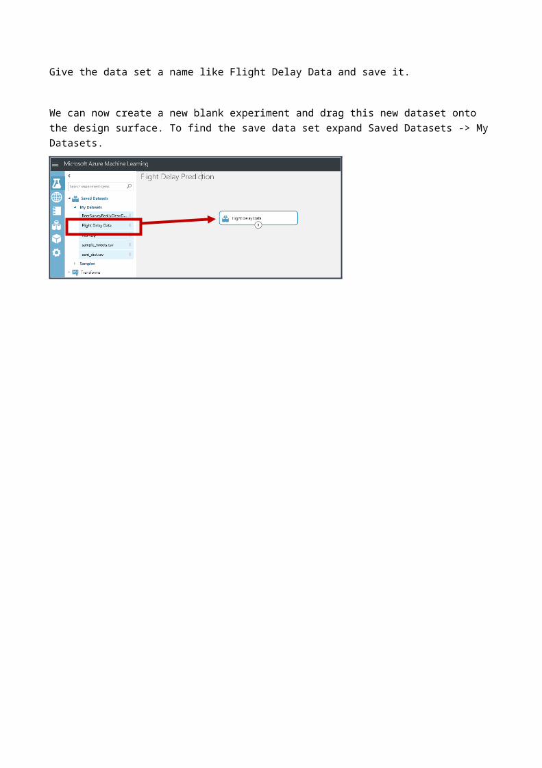
Give the data set a name like Flight Delay Data and save it.

Save the Dataset

We can now create a new blank experiment and drag this new dataset onto the design surface. To find the save data set expand Saved Datasets -> My Datasets.

At this point in the experimentation process we have a clean set of data that can be used to train and evaluate a model. We are moving from the business knowledge domain to the machine learning domain. To predict if a flight is delayed or not based on historical data sets, this experiment is a form of supervised learning and we will apply binary classification models to the data to predict if a flight is delayed or not.Check out the ‘Key Word Definitions’ section at the bottom of this document for machine learning term explanations

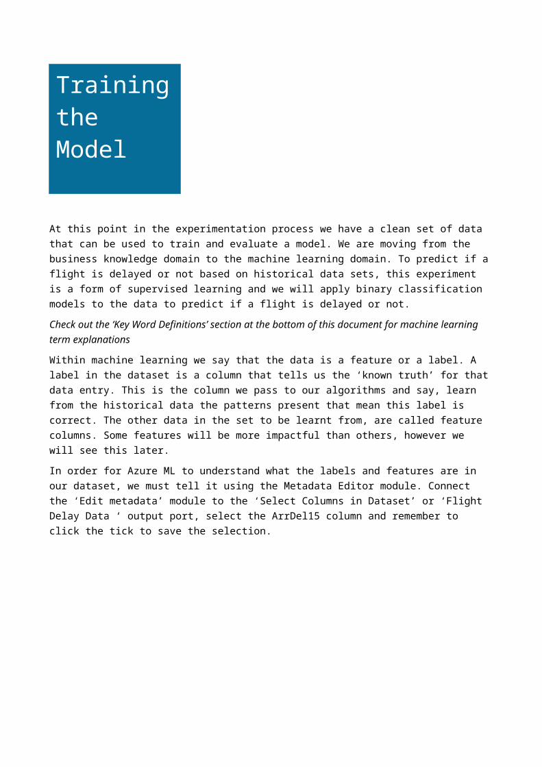
Within machine learning we say that the data is a feature or a label. A label in the dataset is a column that tells us the ‘known truth’ for that data entry. This is the column we pass to our algorithms and say, learn from the historical data the patterns present that mean this label is correct. The other data in the set to be learnt from, are called feature columns. Some features will be more impactful than others, however we will see this later.In order for Azure ML to understand what the labels and features are in our dataset, we must tell it using the Metadata Editor module. Connect the ‘Edit metadata’ module to the ‘Select Columns in Dataset’ or ‘Flight Delay Data ‘ output port, select the ArrDel15 column and remember to click the tick to save the selection.

Training the Model

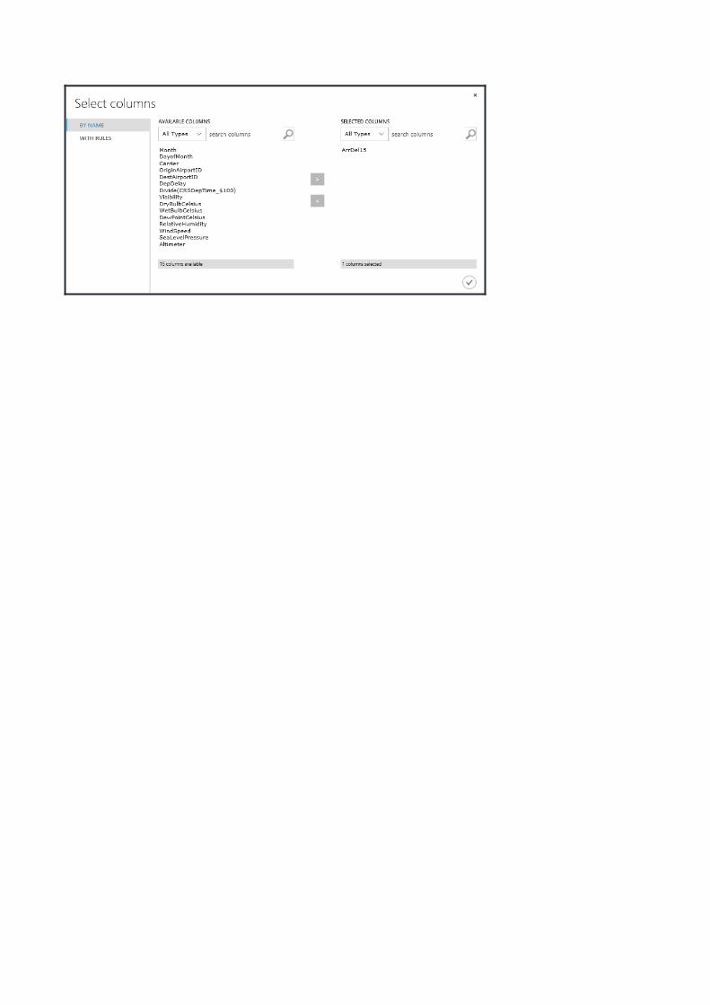
In this lab we want the classifier to learn the behaviour of ‘ArrDelay15’ therefore in the ‘Fields’ parameter select ‘Label’.

Finally, we need to tell Azure ML that the rest of the columns in the set are features and it should find patterns in this data that effect the ArrDel15 column. Drag another ‘Edit Metadata’ module onto the design surface and edit its properties as follows. In the Select columns dialog select “WITH RULES”, Begin with all columns and ‘Exclude’ all labels. Set the Fields property of the ‘Edit Metadata’ module to ‘Features’.

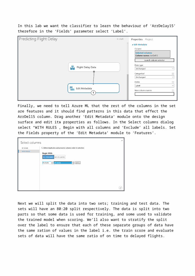
Next we will split the data into two sets; training and test data. The sets will have an 80:20 split respectively. The data is split into two parts so that some data is used for training, and some used to validate the trained model when scoring. We’ll also want to stratify the split over the label to ensure that each of these separate groups of data have the same ration of values in the label i.e. the train score and evaluate sets of data will have the same ratio of on time to delayed flights.

Drag and drop the first split module onto the workspace. Connect this to the project columns module and set the ‘fraction of rows in the first output dataset’ field to 0.8 (80%). Set the “Stratified Split” option to True and set the stratification key column to all labels.

After splitting the data, choose a classifier from the module list in the left hand menu. There are many classifiers depending on your prediction problem and the type of learning you want to use. In the accompanying deck with this lab there is a cheat sheet on which algorithm to use. For this lab we will use the ‘Two-Class Logistic Regression’ classifier module. Drag and drop this onto the workspace.

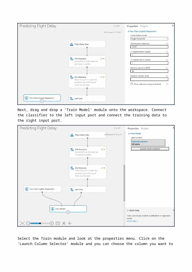
Next, drag and drop a ‘Train Model’ module onto the workspace. Connect the classifier to the left input port and connect the training data to the right input port.

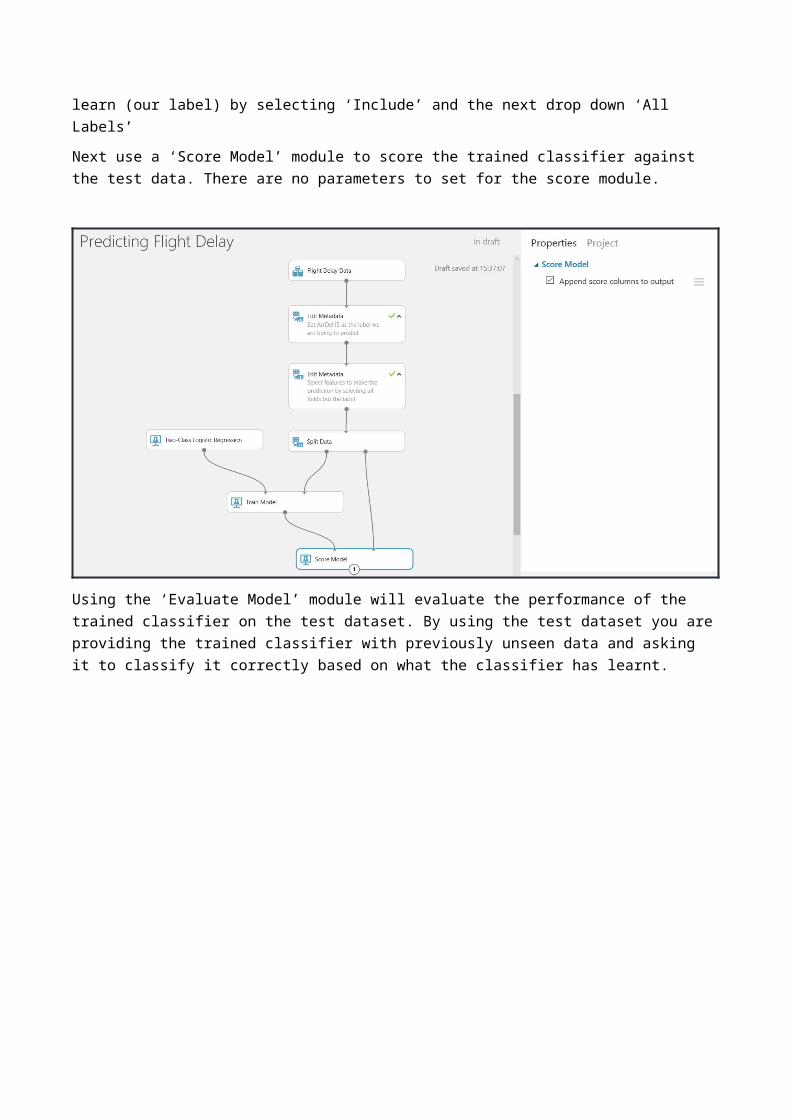
Select the Train module and look at the properties menu. Click on the ‘Launch Column Selector’ module and you can choose the column you want to learn (our label) by selecting ‘Include’ and the next drop down ‘All Labels’

Next use a ‘Score Model’ module to score the trained classifier against the test data. There are no parameters to set for the score module.

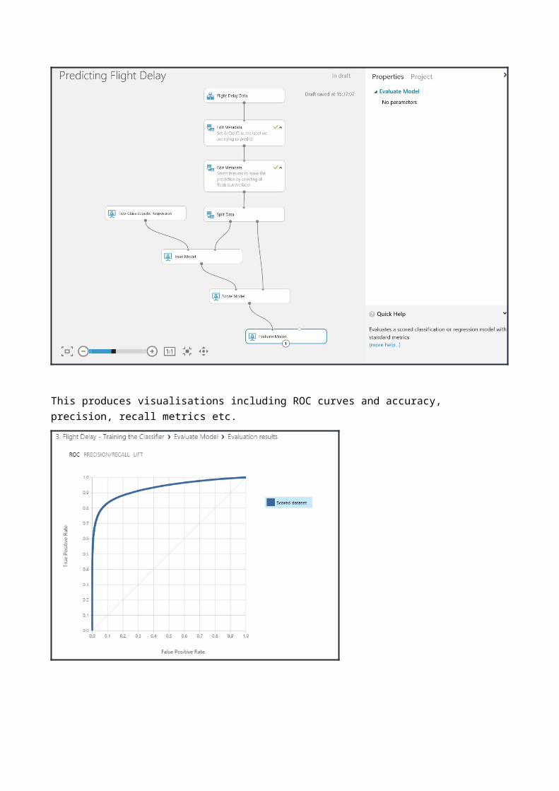
Using the ‘Evaluate Model’ module will evaluate the performance of the trained classifier on the test dataset. By using the test dataset you are providing the trained classifier with previously unseen data and asking it to classify it correctly based on what the classifier has learnt.

This produces visualisations including ROC curves and accuracy, precision, recall metrics etc.

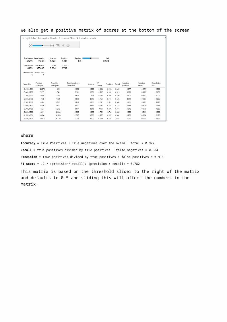
We also get a positive matrix of scores at the bottom of the screen

Where Accuracy = True Positives + True negatives over the overall total = 0.922Recall = true positives divided by true positives + false negatives = 0.684 Precision = true positives divided by true positives + false positives = 0.913F1 score = .2 * (precision* recall)/ (precision + recall) = 0.782

This matrix is based on the threshold slider to the right of the matrix and defaults to 0.5 and sliding this will affect the numbers in the matrix.

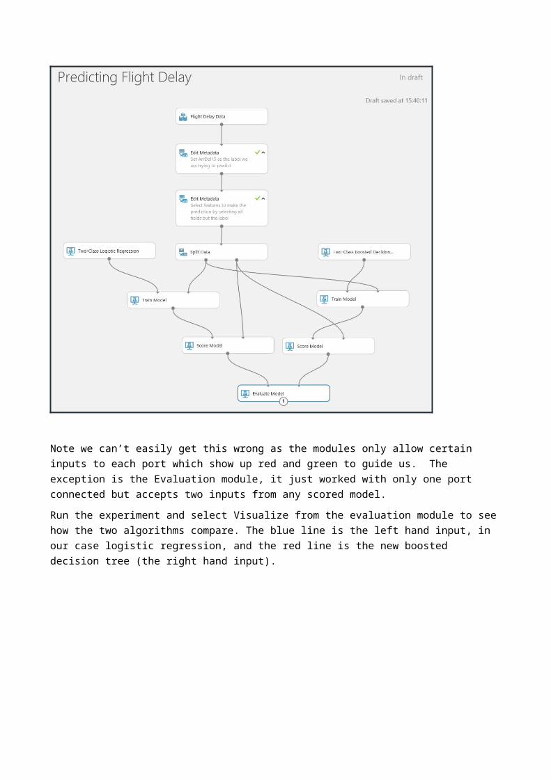
Currently we have one classifier and its evaluation metrics. A great feature of Azure ML studio is that you can very easily compare multiple classifiers.In this section we will compare the Logistic Regression classifier against the Boosted Decision Tree classifier to see which one best suits the data for our prediction.Find the ‘Two-Class Boosted Decision Tree’ classifier and drag this onto the workspace. Notice in the properties pane there are many parameters you can set for each classifier. It is hard to optimise parameters manually, we will see later on in the lab how to optimise the parameters.To speed things up lasso the train and score modules copy and paste them back onto the design surface and wire them up as shown below.

Optimizing Classifiers

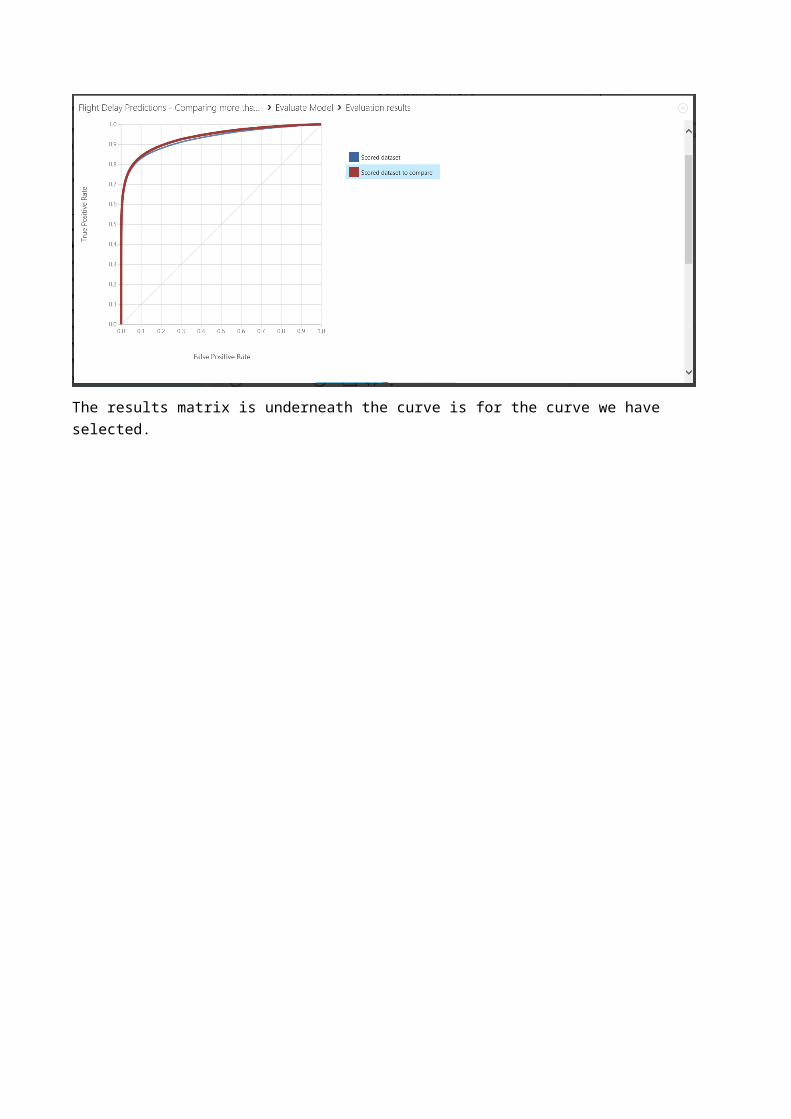
Note we can’t easily get this wrong as the modules only allow certain inputs to each port which show up red and green to guide us. The exception is the Evaluation module, it just worked with only one port connected but accepts two inputs from any scored model. Run the experiment and select Visualize from the evaluation module to see how the two algorithms compare. The blue line is the left hand input, in our case logistic regression, and the red line is the new boosted decision tree (the right hand input).

The results matrix is underneath the curve is for the curve we have selected.

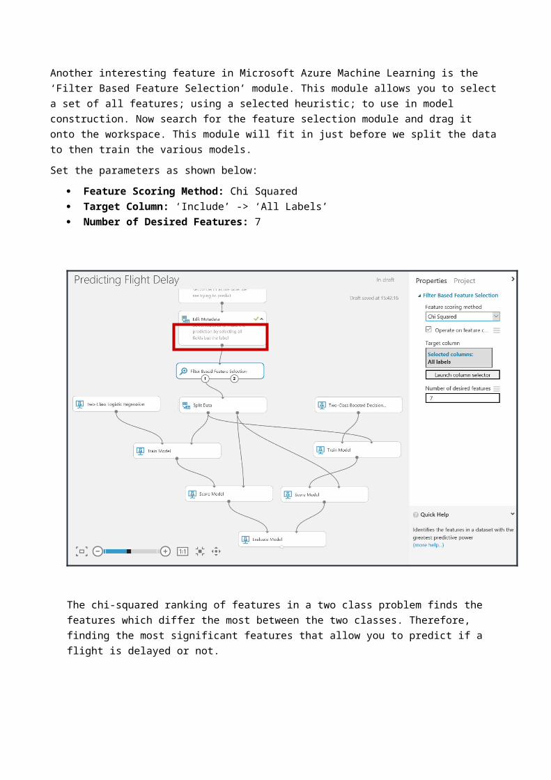
Another interesting feature in Microsoft Azure Machine Learning is the ‘Filter Based Feature Selection’ module. This module allows you to select a set of all features; using a selected heuristic; to use in model construction. Now search for the feature selection module and drag it onto the workspace. This module will fit in just before we split the data to then train the various models.Set the parameters as shown below:

Feature Scoring Method: Chi Squared Target Column: ‘Include’ -> ‘All Labels’ Number of Desired Features: 7

The chi-squared ranking of features in a two class problem finds the features which differ the most between the two classes. Therefore, finding the most significant features that allow you to predict if a flight is delayed or not.

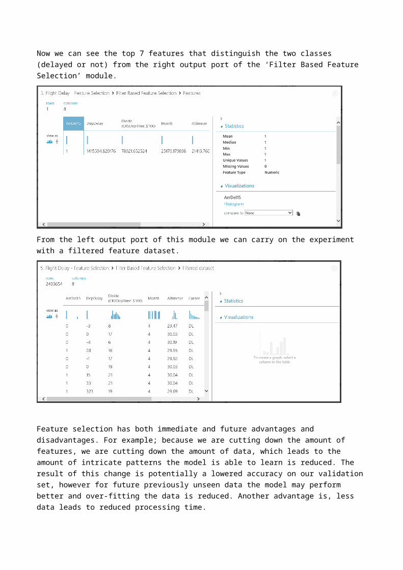
Now we can see the top 7 features that distinguish the two classes (delayed or not) from the right output port of the ‘Filter Based Feature Selection’ module.

From the left output port of this module we can carry on the experiment with a filtered feature dataset.

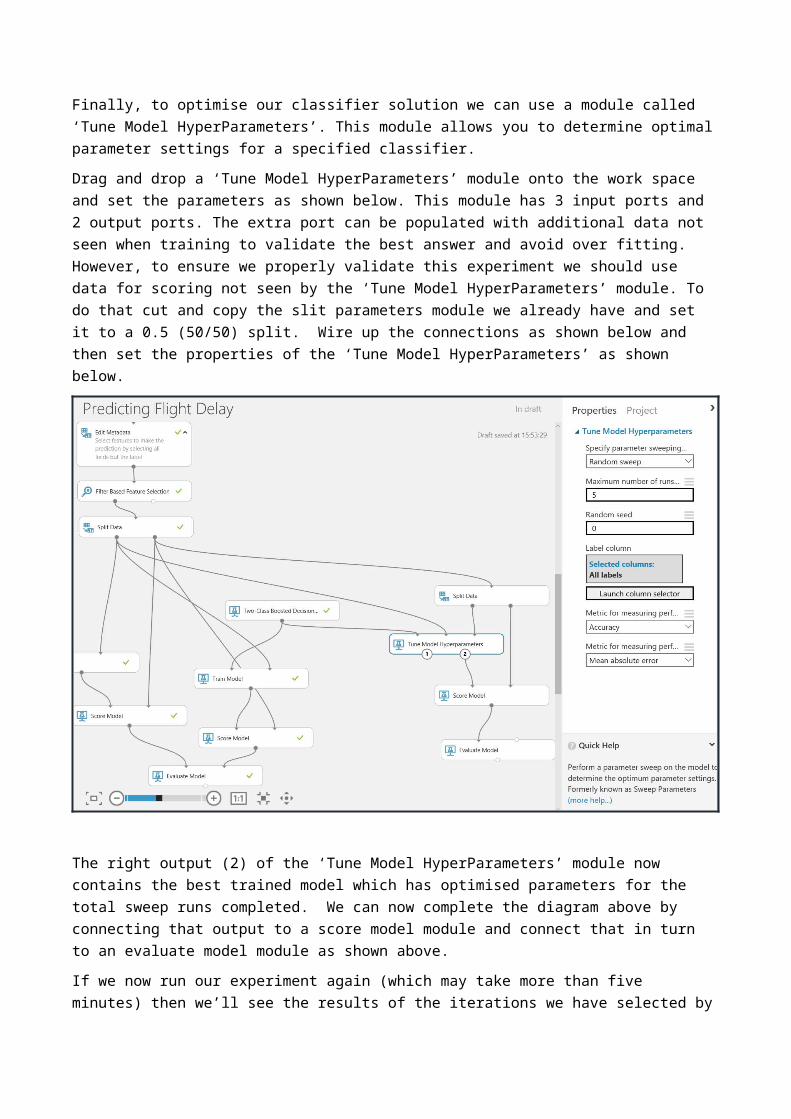
Feature selection has both immediate and future advantages and disadvantages. For example; because we are cutting down the amount of features, we are cutting down the amount of data, which leads to the amount of intricate patterns the model is able to learn is reduced. The result of this change is potentially a lowered accuracy on our validation set, however for future previously unseen data the model may perform better and over-fitting the data is reduced. Another advantage is, less data leads to reduced processing time.Finally, to optimise our classifier solution we can use a module called ‘Tune Model HyperParameters’. This module allows you to determine optimal parameter settings for a specified classifier.

Drag and drop a ‘Tune Model HyperParameters’ module onto the work space and set the parameters as shown below. This module has 3 input ports and 2 output ports. The extra port can be populated with additional data not seen when training to validate the best answer and avoid over fitting. However, to ensure we properly validate this experiment we should use data for scoring not seen by the ‘Tune Model HyperParameters’ module. To do that cut and copy the slit parameters module we already have and set it to a 0.5 (50/50) split. Wire up the connections as shown below and then set the properties of the ‘Tune Model HyperParameters’ as shown below.

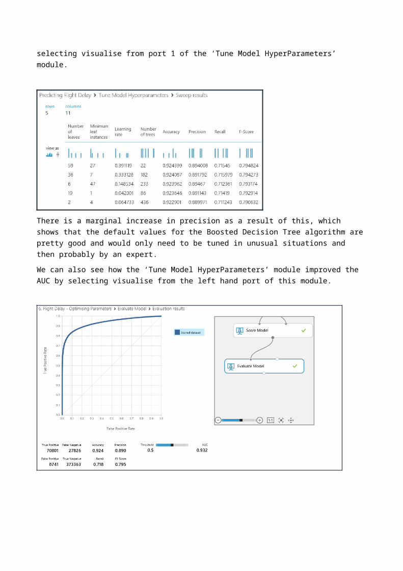
The right output (2) of the ‘Tune Model HyperParameters’ module now contains the best trained model which has optimised parameters for the total sweep runs completed. We can now complete the diagram above by connecting that output to a score model module and connect that in turn to an evaluate model module as shown above.If we now run our experiment again (which may take more than five minutes) then we’ll see the results of the iterations we have selected by selecting visualise from port 1 of the ‘Tune Model HyperParameters’ module.

There is a marginal increase in precision as a result of this, which shows that the default values for the Boosted Decision Tree algorithm are pretty good and would only need to be tuned in unusual situations and then probably by an expert.We can also see how the ‘Tune Model HyperParameters’ module improved the AUC by selecting visualise from the left hand port of this module.

That shows how we can use the more advanced features in Azure ML to tune our model and assess how successful it is. Do bear in mind that this depends on what success looks like, for example:

Accuracy at any cost Speed The best result using the minimum amount of data is it accuracy.

There is no right answer here it depends on the business problem we are trying to solve.

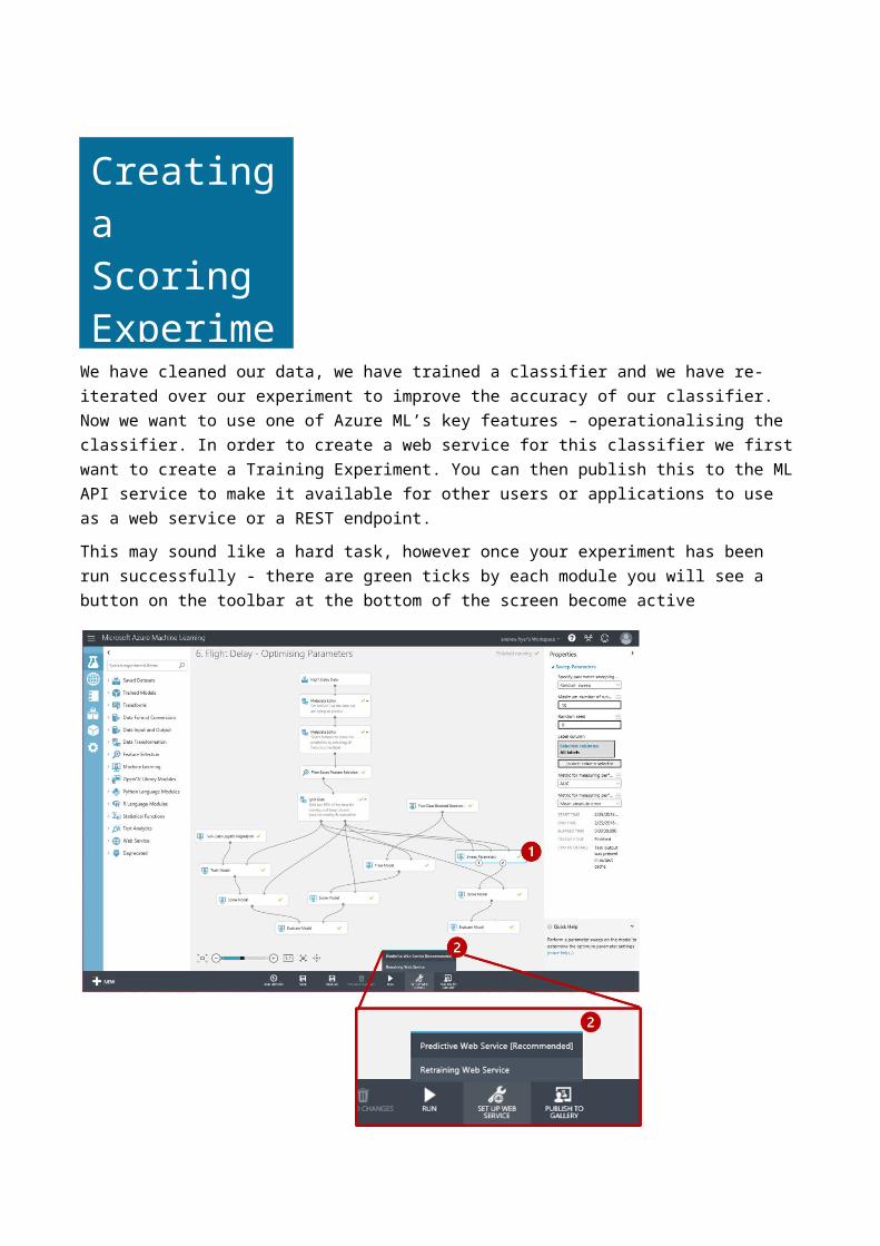
We have cleaned our data, we have trained a classifier and we have re-iterated over our experiment to improve the accuracy of our classifier. Now we want to use one of Azure ML’s key features – operationalising the classifier. In order to create a web service for this classifier we first want to create a Training Experiment. You can then publish this to the ML API service to make it available for other users or applications to use as a web service or a REST endpoint.This may sound like a hard task, however once your experiment has been run successfully - there are green ticks by each module you will see a button on the toolbar at the bottom of the screen become active

*Note:* Make sure you select the module that you want the studio to save as your best trained model. In this case we select the ‘Tune Model HyperParameters’ module.

Creating a Scoring Experiment

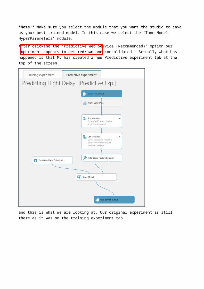
After clicking the ‘Predictive Web Service (Recommended)’ option our experiment appears to get redrawn and consolidated. Actually what has happened is that ML has created a new Predictive experiment tab at the top of the screen.

and this is what we are looking at. Our original experiment is still there as it was on the training experiment tab.

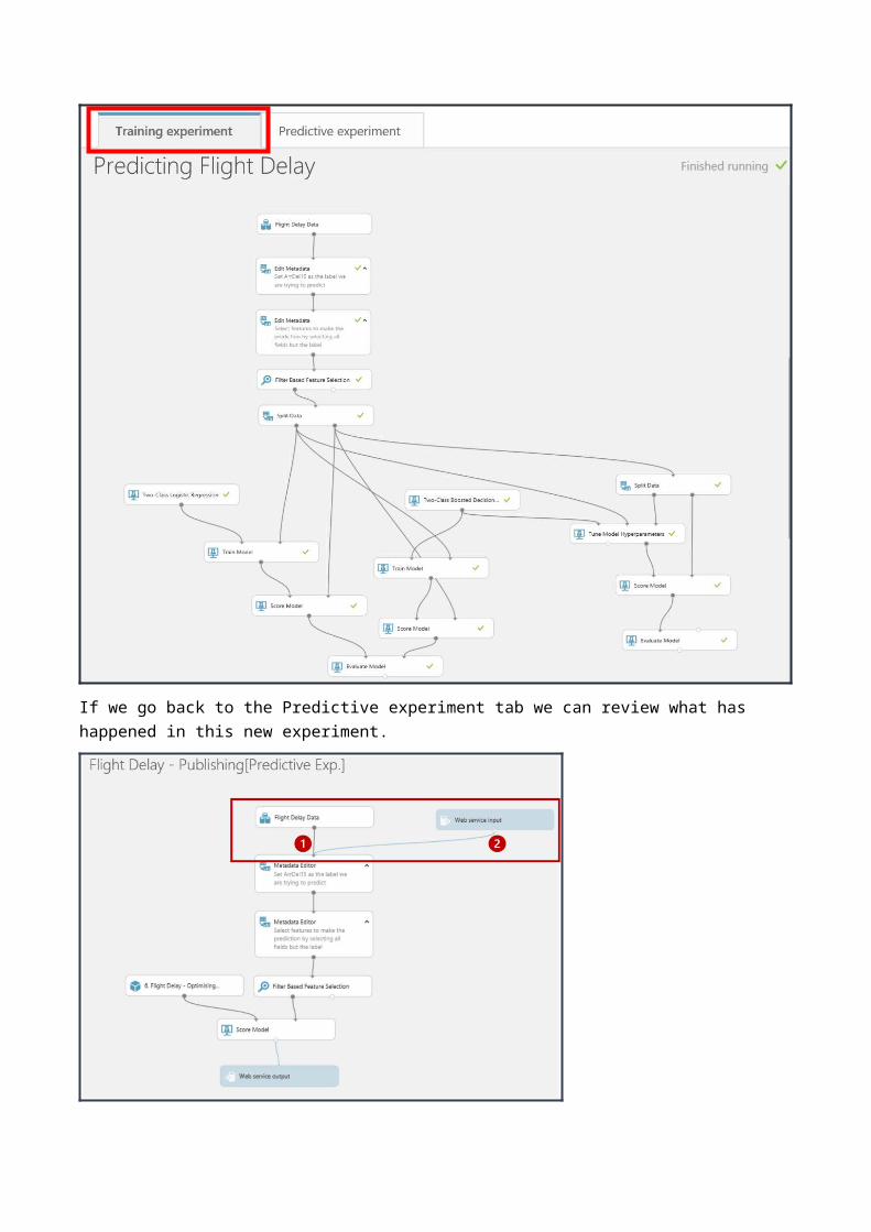
If we go back to the Predictive experiment tab we can review what has happened in this new experiment.

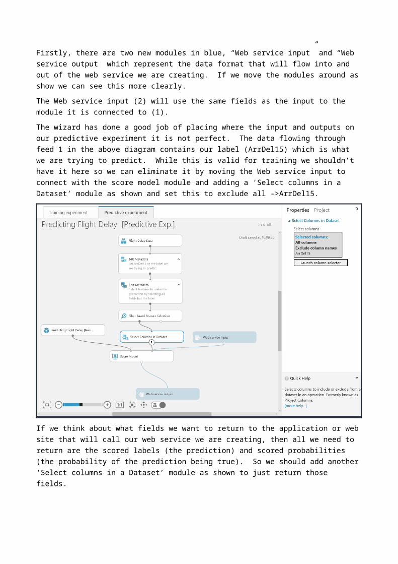
Firstly, there are two new modules in blue, “Web service input” and “Web service output” which represent the data format that will flow into and out of the web service we are creating. If we move the modules around as show we can see this more clearly.The Web service input (2) will use the same fields as the input to the module it is connected to (1).The wizard has done a good job of placing where the input and outputs on our predictive experiment it is not perfect. The data flowing through feed 1 in the above diagram contains our label (ArrDel15) which is what we are trying to predict. While this is valid for training we shouldn’t have it here so we can eliminate it by moving the Web service input to connect with the score model module and adding a ‘Select columns in a Dataset’ module as shown and set this to exclude all ->ArrDel15.

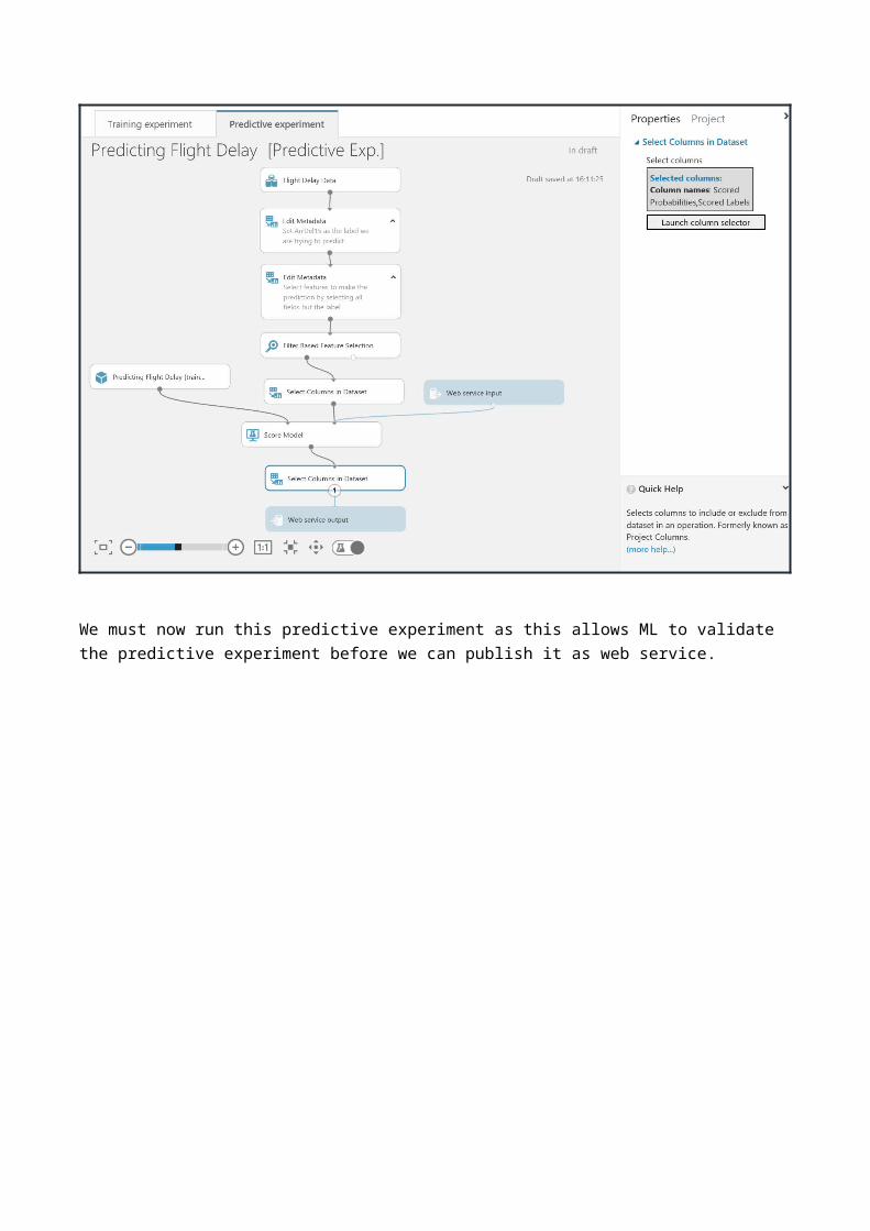
If we think about what fields we want to return to the application or web site that will call our web service we are creating, then all we need to return are the scored labels (the prediction) and scored probabilities (the probability of the prediction being true). So we should add another ‘Select columns in a Dataset’ module as shown to just return those fields.

We must now run this predictive experiment as this allows ML to validate the predictive experiment before we can publish it as web service.

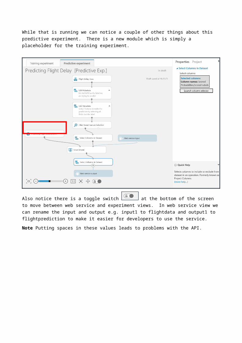
While that is running we can notice a couple of other things about this predictive experiment. There is a new module which is simply a placeholder for the training experiment.

Also notice there is a toggle switch at the bottom of the screen to move between web service and experiment views. In web service view we can rename the input and output e.g. input1 to flightdata and output1 to flightprediction to make it easier for developers to use the service. Note Putting spaces in these values leads to problems with the API.

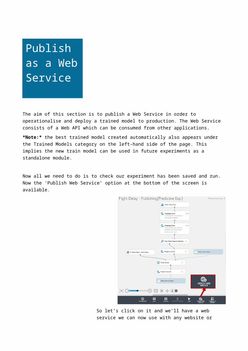
The aim of this section is to publish a Web Service in order to operationalise and deploy a trained model to production. The Web Service consists of a Web API which can be consumed from other applications. *Note:* the best trained model created automatically also appears under the Trained Models category on the left-hand side of the page. This implies the new train model can be used in future experiments as a standalone module.

Now all we need to do is to check our experiment has been saved and run. Now the ‘Publish Web Service’ option at the bottom of the screen is available.

So let’s click on it and we’ll have a web service we can now use with any website or application capable of making a call to a rest api.

Publish as a Web Service

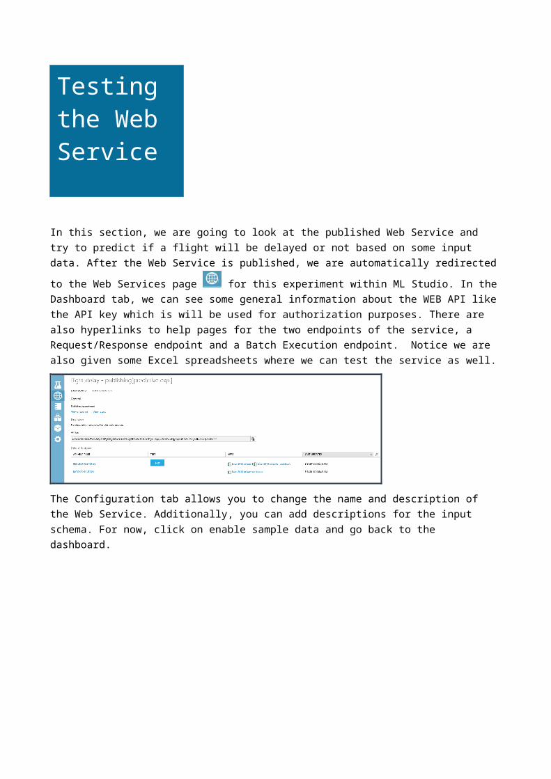
In this section, we are going to look at the published Web Service and try to predict if a flight will be delayed or not based on some input data. After the Web Service is published, we are automatically redirected to the Web Services page for this experiment within ML Studio. In the Dashboard tab, we can see some general information about the WEB API like the API key which is will be used for authorization purposes. There are also hyperlinks to help pages for the two endpoints of the service, a Request/Response endpoint and a Batch Execution endpoint. Notice we are also given some Excel spreadsheets where we can test the service as well.

The Configuration tab allows you to change the name and description of the Web Service. Additionally, you can add descriptions for the input schema. For now, click on enable sample data and go back to the dashboard.

Testing the Web Service

On the Dashboard tab click on the button alongside the REQUEST/RESPONSE API as a quick sense check to see if our web service is working as expected.Enter the following values in the Enter data to predict dialog:

DepDelay = 33 Divide(CRSDEPTIME_$100) = 8 Month = 4 Altimeter = 29.6 Carrier = DL SeaLevelPressure 30 DewPointCelcius = 1.7

The result you receive back after processing returns a JSON like output.

Notice we just get back the Scored Label and the Scored Probabilities. So in the case below we can say that given the parameters above the classifier has predicted the flight will be more than 15 mins delayed (1) and it is very confident in its decision (0.997861325740814).We can also use the excel add-ins to test the web site and there is also a partially configured web site in the Azure Web App Marketplace. Simply go to the site and look for Azure ML.This will create a web app in our azure subscription.

If we then click on the URL of the new site we’ll be presented with a simple page where we can enter our API URL and API key ..

The key is on the API dashboard and the URL is at the top of the Request response page. Click Submit and close the page. Go back to the Azure Portal and open the site again and enter some trial values..

Optionally try the Excel spreadsheet to see how that works if you have Excel on your machine. Below is what the Excel 2013 version looks like which uses the new Excel add-ins to automatically setup a connection to the API we have and also allows us to use sample data to test.

The most recent release of Azure ML includes a community-driven gallery that lets you discover and use interesting experiments authored by others. You can ask questions or post comments about experiments in the gallery and more importantly publish your own!The gallery is a great way for users to get started with Azure Machine Learning and learn from others in the community: https://gallery.azureml.net/

You can access this gallery via the URL above, or if you are already in the studio you can click the ‘Gallery’ option in the top toolbar:

Publish to the Gallery

In order to publish your own experiment, you need to have met the conditions below:1. You have created an experiment in Azure ML Studio2. Your experiment runs (all green ticks)3. You have created a web service and scoring experimentIt is that easy! So everything we have done in this lab has meant that we could publish our experiments in the Gallery. As you will notice in your experiment workspace the ‘Publish to Gallery’ option in the bottom toolbar has become available

This will take you through various stages to Name, give a description, image and tags for your experiment. Then publish it to the Gallery for you.

The experiment we have created in this lab is now available in two forms in the gallery. Check them out here:Flight Delay Pre-processing stage: https://gallery.azureml.net/Details/cc618dd8dfb14af0a6354c01ffd606e6

Flight Delay Web Service stage: https://gallery.azureml.net/Details/bc3008585f374b62be54d4e57ae8a240

This lab was intended to introduce you to the basic concepts of Machine Learning such as binary classification, feature selection, training and testing a model and using Azure Machine Learning. A web service was created to operationalize and deploy the model for production.

Next Steps: Check out the UK Data Developer page on MSDN here:

Check out the Azure ML Gallery and download and edit/run other types of machine learning experiments: https://gallery.azureml.net/

Also check out other Azure Services that can be used with Machine Learning such as HDInsight, Data Factory and Stream Analytics: http://azure.microsoft.com/en-us/services/

Conclusion