Raven: Scheduling Virtual Machine Migration during

Manuscript No. MONE-D-20-00162R1

Raven : Scheduling Virtual Machine Migrationduring Datacenter Upgrades with Reinforcement Learning

Chen Ying · Baochun Li · Xiaodi Ke · Lei Guo

the date of receipt and acceptance should be inserted later

Abstract Physical machines in modern datacenters are

routinely upgraded due to their maintenance require-

ments, which involve migrating all the virtual machines

they currently host to alternative physical machines.

For this kind of datacenter upgrades, it is critical to

minimize the time it takes to upgrade all the physical

machines in the datacenter, so as to reduce disruptions

to cloud services. To minimize the upgrade time, it is

essential to carefully schedule the migration of virtual

machines on each physical machine during its upgrade,

without violating any constraints imposed by virtual

machines that are currently running. Rather than re-

sorting to heuristic algorithms as existing work, we pro-

pose a new scheduler, Raven, that uses an experience-

driven approach with deep reinforcement learning to

schedule the virtual machine migration. With our de-

sign of the state space, action space and reward func-

tion, Raven trains a fully-connected neural network us-

ing the cross-entropy method to approximate the policy

of choosing a destination physical machine for each vir-

tual machine before its migration. We compare Raven

with state-of-the-art algorithms in the literature, and

our results show that Raven can effectively shorten the

Chen YingUniversity of TorontoE-mail: [email protected]

Baochun LiUniversity of TorontoE-mail: [email protected]

Xiaodi KeHuawei CanadaE-mail: [email protected]

Lei GuoHuawei CanadaE-mail: [email protected]

time to complete the datacenter upgrade under differ-

ent datacenter settings.

Keywords Virtual machine migration · Deep rein-

forcement learning

1 Introduction

In a modern datacenter, it is routine for its physical

machines to be upgraded to newer versions of operat-

ing systems or firmware versions from time to time, as

part of their maintenance. However, production data-

centers are used for hosting virtual machines, and these

virtual machines will have to be migrated to alternative

physical machines during the upgrade process. The mi-

gration process takes time, which involves transferring

the images of virtual machines between physical ma-

chines across the datacenter network.

To incur the least amount of disruption to cloud

services provided by a production datacenter, it is com-

monly accepted that we need to complete the upgrade

process as quickly as possible. Assuming that the time

of upgrading a physical machine is dominated by the

time it takes to migrate the images of all the virtual

machines on this physical machine, the problem of min-

imizing the upgrade time of all physical machines in a

datacenter is equivalent to minimizing the total migra-

tion time, which is the time it takes to finish all the

virtual machine migrations during the datacenter up-

grade.

In order to reduce the total migration time, we will

need to plan the schedule of migrating virtual machines

carefully. To be more specific, we should carefully select

the best possible destination physical machine for each

virtual machine to be migrated. However, as it is more

2 Chen Ying et al.

realistic to assume that the topology of the datacen-

ter network and the network capacity on each link are

unknown to such a scheduler, computing the optimal

migration schedule that minimizes the total migration

time becomes more challenging.

With the objective of minimizing the migration time,

a significant amount of work on scheduling the migra-

tion of virtual machines has been proposed. However, to

the best of our knowledge, none of them considered the

specific problem of migrating virtual machines during

datacenter upgrades. Commonly, existing studies focus

on migrating a small number of virtual machines to re-

duce the energy consumption of physical machines [1]

[2] [3], or to balance the utilization of different resources

across physical machines [4]. Further, most of the pro-

posed schedulers are based on heuristic algorithms and

a set of strong assumptions that may not be realized in

practice.

Without such detailed knowledge of the datacenter

network, we wish to explore the possibilities of making

scheduling decisions based on deep reinforcement learn-

ing [5], which trains an agent to learn the policy with

a deep neural network as the function approximator to

make better decisions from its experience, as it inter-

acts with an unknown environment. Though it has been

shown that deep reinforcement learning is effective in

playing games [6], whether it is suitable for scheduling

resources, especially in the context of scheduling migra-

tion of virtual machines, is not generally known.

In this paper, we propose Raven, a new scheduler for

scheduling the migration of virtual machines in the spe-

cific context of datacenter upgrades. In contrast to ex-

isting work in the literature, we assume that the topol-

ogy and link capacities of the datacenter network are

not known a priori to the scheduler, which is more

widely applicable to realistic scenarios involving pro-

duction datacenters. By considering the datacenter net-

work as an unknown environment that needs to be

explored, we seek to leverage reinforcement learning

to train an agent to choose an optimal scheduling ac-

tion, i.e., the best destination physical machine for each

virtual machine to be migrated, with the objective of

achieving the shortest possible total migration time for

the datacenter upgrade. By tailoring the state space, ac-

tion space and reward function for our scheduling prob-

lem, Raven uses the off-the-shelf cross-entropy method

to train a fully-connected neural network to approxi-

mate the policy of choosing a destination physical ma-

chine for each virtual machine before its migration, aim-

ing at minimizing the total migration time.

Highlights of our original contributions in this paper

are as follows. First, we consider the real-world problem

of migrating virtual machines for upgrading physical

machines in a datacenter, which is rarely studied in the

previous work. Second, we design the state space, action

space, and reward function for our deep reinforcement

learning agent to schedule the migration of virtual ma-

chines with the objective of minimizing the total mi-

gration time. Finally, we propose and implement our

new scheduler, Raven, and conduct a collection of sim-

ulations to show Raven’s effectiveness of outperforming

the existing methods with respect to minimizing the to-

tal migration time, without any a priori knowledge of

the datacenter network under different datacenter set-

tings.

2 Problem Formulation and Motivation

To start with, we consider two different resources, CPU

and memory, and we assume the knowledge of both

the number of CPUs and the size of the main mem-

ory in each of the virtual machines (VMs) and physical

machines (PMs). In addition, we assume that the cur-

rent mapping between the VMs and PMs is known as

well, in that for each PM, we know the indexes of the

VMs that are currently hosted there. It is commonly

accepted that the number of CPUs and the size of the

main memory of every VM on a PM can be accommo-

dated by the total number of physical CPUs and the

total size of physical memory on this hosting PM.

Firstly, we use an example to illustrate the way

of computing the migration time of a migration batch.

Some migration processes can be conducted at the same

time, if 1) for all these migration processes, no source

PM is the same as any destination PM and no desti-

nation PM is the same as any source PM and 2) every

destination PM in these migration processes has enough

residual CPUs and memory to host all VMs that will

be migrated to it. We treat migration processes that

can process at the same time as a migration batch.

Core Switch

AggregationSwitch #0

PM #0 PM #1 PM #2

AggregationSwitch #1

PM #4 PM #5PM #3

Fig. 1: The network topology of the example.

Fig. 1 shows the assumed network topology. There

are 6 PMs, with PM #0 to PM #2 linked to AS (ag-

gregation switch) # 0, and PM #3 to PM #5 linked to

AS #1. AS #0 and AS #1 connect to the core switch.

Raven: Scheduling Virtual Machine Migration during Datacenter Upgrades with Reinforcement Learning 3

Assume that the network capacity of each link be-

tween an aggregation switch and the core switch is

1GB/s, and the network capacity of each link between

a PM and an AS is 2GB/s.

Take computing the migration time of a migration

batch with three migration processes as an example:

♦ VM #0 (with 1GB of image): PM #0 → PM #3



According to the network topology, the route of each

migration process is:

♦ VM #0: PM #0 → AS #0 → core switch → AS #1

→ PM #3

♦ VM #1: PM #0 → AS #0 → PM #1

♦ VM #2: PM #0 → AS #0 → core switch → AS #1

→ PM #5

In the beginning, all these three migration processes

proceed at the same time, and we assume that every

migration process using the same bottleneck link gets

equal throughput. So the bandwidth of each possible

bottleneck link is:

PM #0 → AS #0: 23GB/s;

AS #0 → core switch: 12GB/s.

Thus the migration rate of VM #1 is 23GB/s, while

VM #0 and VM #2 are both 12 GB/s.

To complete the migration with these rates, the time

needed by each VM is:

VM #0: 1GB / ( 12GB/s) = 2s;

VM #1: 2GB / ( 23GB/s) = 3s;

VM #2: 3GB / ( 12GB/s) = 6s.

As VM #0 takes the minimal time of 2s, the band-

width of every link might change after 2s.

In the first 2s, VM #1 transfers 2s × 23GB/s = 4

3GB

size of image. It needs to transfer 23GB later. VM #2

finishes transferring 2s × 12GB/s = 1GB, with 2GB left.

Starting from 2s, the bandwidth of each possible

bottleneck link is:

PM #0 → AS #0: 1GB/s;


So the rates of VM #1 and VM #2 are both 1GB/s.

VM #1 can finish its migration in 23GB / (1GB/s)

= 23 s. After that, VM #2 will be the only VM whose

migration has not finished. In this 23 s, VM #2 transfers

23GB of image, remaining 4

3GB to be transferred.

Starting from 2s + 23 s, the bandwidth of each pos-

sible bottleneck link is:

PM #0 → AS #0: 2GB/s;


So the migration rate of VM #2 is 1GB/s, and thus

VM #2 finishes its migration in 43GB / (1GB/s) = 4

3 s.

Therefore, the migration time of this migration batch

is 2s + 23 s +

43 s = 4s.

Now, we use the following example to illustrate the

upgrade process of the physical machines, and to ex-

plain why the problem of scheduling VM migrations to

minimize the total migration time may be non-trivial.

Assume there are three PMs in total, each hosting

one of the three VMs. The information of these PMs

and VMs, with respect to the number of CPUs and the

amount of memory, are shown in Fig. 2. These PMs are

updated one by one. To show the total migration times

of different schedules, we assume the simplest possible

datacenter network topology, where all of these three

PMs are connected to the same core switch, and the

network capacity of the link between the core switch

and each PM is 1GB/s.

In the first schedule, as shown in Fig. 2, we first

upgrade PM #0 and migrate VM #0 to PM #2, and

then upgrade PM #1 by migrating VM #1 to PM #2.

Finally, we upgrade PM #2 with migrating VM #0,

VM # 1 and VM # 2 to PM #0.

From the perspective of VMs, the migration process

of each VM is:

♦ VM #0: PM #0 → PM #2 → PM #0;

♦ VM #1: PM #1 → PM #2 → PM #0;

♦ VM #2: PM #2 → PM #0.

To calculate the total migration time, we start from

the VM on the PM that is upgraded first. In this sched-

ule, we start from the migration of VM #0 from PM

#0 to PM #2. As PM #0 is being upgraded now, we

cannot migrate VM #1 or VM #2, whose destination

PM is PM #0. Since only VM #0 is being migrated, it

can use all the network capacity through the link in its

migration. This migration takes 1GB/(1GB/s) = 1s.

Then we come to VM #1 as PM #1 is upgraded

next. Now the rest of migration processes whose migra-

tion times have not been calculated are:

♦ VM #0: PM #2 → PM #0;

♦ VM #1: PM #1 → PM #2 → PM #0;

♦ VM #2: PM #2 → PM #0.

As VM #1 is migrated to PM #2, here we cannot

migrate VM #0 or VM #2, whose source PM is PM

#2. Since only VM #1 is being migrated, it can occupy

all the network capacity through the link during its

migration. This migration takes 2GB/(1GB/s) = 2s.

At last, we come to PM#2. All unfinished migration

processes are:

♦ VM #0: PM #2 → PM #0;

♦ VM #1: PM #2 → PM #0;

♦ VM #2: PM #2 → PM #0.

Apparently, all these three migration processes can

be conducted in one migration batch. Since at first,

4 Chen Ying et al.

VM #0 ��&38��*%�PHPRU\�

VM #1 ��&38��*%�PHPRU\�

VM #0 ��&38��*%�PHPRU\�VM #2 ��&38V��*%�PHPRU\�

PM #04 CPUs, 8GB memory



VM #1 ��&38��*%�PHPRU\�

VM #0 ��&38��*%�PHPRU\�VM #1 ��&38��*%�PHPRU\�

VM #2 ��&38V��*%�PHPRU\�

Upgrade PM #0 Upgrade PM #1 Upgrade PM #2

VM #2 ��&38V��*%�PHPRU\�VM #0 ��&38��*%�PHPRU\�VM #1 ��&38��*%�PHPRU\�

VM #2 ��&38V��*%�PHPRU\�

Fig. 2: Scheduling VM migration: a schedule that takes 9 seconds of total migration time.

VM #0 ��&38��*%�PHPRU\�

VM #1 ��&38��*%�PHPRU\�

VM #2 ��&38V��*%�PHPRU\�




VM #0 ��&38��*%�PHPRU\�VM #1 ��&38��*%�PHPRU\�

VM #2 ��&38V��*%�PHPRU\�

VM #0 ��&38��*%�PHPRU\�

VM #1 ��&38��*%�PHPRU\�VM #2 ��&38V��*%�PHPRU\�

Upgrade PM #0 Upgrade PM #2 Upgrade PM #1

VM #2 ��&38V��*%�PHPRU\�

VM #0 ��&38��*%�PHPRU\�VM #1 ��&38��*%�PHPRU\�

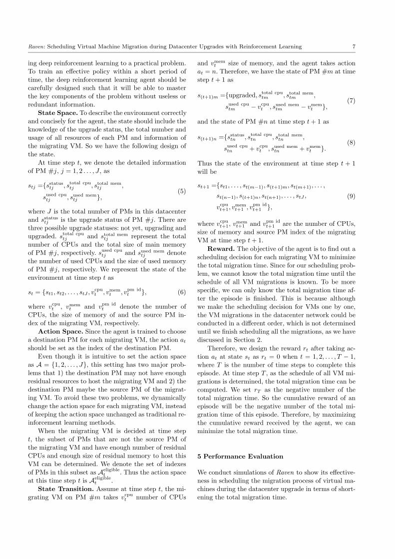
Fig. 3: Scheduling VM migration: a schedule that takes 7 seconds of total migration time.

these three VMs share the link from the core switch

to PM #0, each of them will get the rate of 13GB/s.

To finish migrating each VM with this rate, VM #0

will take 1GB/( 13GB/s) = 3s, while VM #1 will take

2GB/( 13GB/s) = 6s, and VM#2 will take 3GB/( 13GB/s)

= 9s. So the migration of VM #0 is completed in 3s.

After 3s, VM #1 and VM #2 share the link from

the core switch to PM #0. Each of them get the rate

of 12GB/s. To finish migrating these two VMs under

this rate, VM #1 will take 1GB/( 12GB/s) = 2s, while

VM #2 will take 2GB/( 12GB/s) = 4s. So we can finish

the migration of VM #1 in 2s. Now, we need to finish

transferring 1GB of the image on VM #2 with the rate

of 1GB/s, which can be done in 1s.

Therefore, the migration time of this migration batch

is 3s + 2s + 1s = 6s. So the total migration time is 1s

+ 2s + 6s = 9s.

In contrast, a better schedule in terms of reducing

the total migration time is shown in Fig. 3. We first

upgrade PM #0 and migrate VM #0 to PM #1, and

then upgrade PM #2 by migrating VM #2 to PM #0.

Finally, we upgrade PM #1 and migrate VM #0 to PM

#2 and VM #1 to VM #0.

From the perspective of VMs, the migration process

of each VM is:

♦ VM #0: PM #0 → PM #1 → PM #2;

♦ VM #1: PM #1 → PM #0.

♦ VM #2: PM #2 → PM #0.

We start from VM #0 which is initially on the first

migrated PM, PM #0. Since the destination PM of VM

#1 is PM #0, which is the source PM of VM #0, the

migration of VM #1 cannot be proceeded now. For the

same reason, the migration of VM #2 cannot be done

either. Therefore, the migration time of migrating VM

#0 from PM #0 to PM #1 is 1GB/(1GB/s) = 1s.

Then we come to VM #2 which is on PM #2, the

next upgraded PM. The migration of VM #1 from PM

#1 to PM #0 can be done at the same time. At first,

These two VMs share the link between the core switch

to PM #0, with 12GB/s. To finish migrating these two

VMs with this rate, VM #1 will take 2GB/( 12GB/s) =

4s, while VM #2 will take 3GB/( 12GB/s) = 6s. So we

can finish the migration of VM #1 in 4s. Now, we need

to finish transferring 1GB of image on VM #2 with

the rate of 1GB/s, which can be done in 1s. Thus, the

migration time of this batch is 4s + 1s = 5s.

At last, we compute the migration time of VM #0

from PM #1 to PM #2, which is 1s. Therefore, the

total migration time of this schedule is 1s + 5s + 1s =


7s, which is shorter than that of the previous schedule

taking 9s.

As we can observe from our examples, even though

we schedule the migration of VMs one by one, the actual

migration order cannot be determined until we have

the schedule of all VM migrations that will take place

during the datacenter upgrade. This implies that we

will only be able to compute the total migration time

when the datacenter upgrade is completed. To make

the scheduling problem even more difficult to solve, it

is much more practical to assume that, unlike our ex-

amples, the topology and network capacities of the dat-

acenter network are not known a priori, which makes it

even more challenging to estimate the total migration

time when scheduling the migration of VMs one by one.

Therefore, we propose to leverage deep reinforce-

ment learning to schedule the destination PM for each

migrating VM, with the objective of minimizing the to-

tal migration time. The hope is that the agent of deep

reinforcement learning can learn to make better deci-

sions by iteratively interacting with an unknown envi-

ronment over time.

3 Preliminaries

Before advancing to our proposed work, we first intro-

duce some preliminaries on deep reinforcement learn-

ing, which applies deep neural networks as function ap-

proximators of reinforcement learning.

Under the standard reinforcement learning setting,

an agent learns by interacting with the environment

E over a number of discrete time steps in an episodic

fashion [5]. During an episode, the agent observes the

state st of the environment at each time step t and

takes an action at from a set of possible actions Aaccording to its policy π : π(a|s) → [0, 1], which is

a probability distribution over actions. π(a|s) is the

probability that action a is taken in state s. Follow-

ing the taken action at, the state of the environment

transits to state st+1 and the agent receives a reward

rt. The process continues until the agent reaches a ter-

minal state. The states, actions, and rewards that the

agent experienced during one episode form a trajectory

x = (s1, a1, r1, s2, a2, r2, · · · , sT , aT , rT ), where T is the

last time step. The cumulative reward R(x) =!T

t=1 rtis used to measure how good a trajectory is.

As the agent’s behaviour is defined by a policy π(a|s),which maps state s to a probability distribution over all

actions a ∈ A, the method of storing the state-action

pairs should be carefully considered. Since the number

of state-action pairs in complex decision-making prob-

lems would be too large to store in tabular form, it is

common to use function approximators, such as deep

neural networks [6] [7] [8] [9]. A function approximator

has a manageable number of adjustable policy param-

eters θ. To show that the policy corresponds to param-

eters θ, we represent it as π(a|s; θ). For the problem

of choosing a destination PM for a migrating VM, an

optimal policy π(a|s; θ∗) with parameters θ∗ is the mi-

gration strategy we want to obtain.

To obtain the parameters θ∗ of an optimal policy,

we could use a basic but efficient method, cross-entropy

[10], whose objective is to maximize the cumulative re-

ward R(x) received in a trajectory x from an arbitrary

set of trajectories X . Denote x∗ as the corresponding

trajectory at which the cumulative reward is maximal,

and let ξ∗ be the maximum cumulative reward, we thus

have R(x∗) = maxx∈X R(x) = ξ∗.

Assume x has the probability density f(x;u) with

parameters u on X , and the estimation of the probabil-

ity that the cumulative reward of a trajectory is greater

than a fixed level ξ is l = P(R(x) ≥ ξ) = E[1{R(x)≥ξ}],

where 1{R(x)≥ξ} = 1 if R(x) ≥ ξ, and 0 otherwise. If ξ

happens to be set closely to the unknown ξ∗, R(x) ≥ ξ

will be a rare event, which requires a large number of

samples to estimate the expectation of its probability

accurately.

A better way to perform the sampling is to use

importance sampling. Let f(x; v) be another proba-

bility density with parameters v such that for all x,

f(x; v) = 0 implies that 1{R(x)≥ξ}f(x;u) = 0. Using

the probability density f(x; v), we can represent l as

l =

"1{R(x)≥ξ}

f(x;u)

f(x; v)f(x; v)dx

= Ex∼f(x;v)

#1{R(x)≥ξ}

f(x;u)

f(x; v)

$.

(1)

Thus the optimal importance sampling probability for

a fixed level ξ is given by f(x; v∗) ∝ |1{R(x)≥ξ} |f(x;u),which is generally difficult to obtain. So the idea of the

cross-entropy method is to choose an importance sam-

pling probability density f(x; v) in a specified class of

densities so that the distance between the optimal im-

portance sampling density f(x; v∗) and f(x; v) is min-

imal. The distance between two probability densities

f1 and f2 could be measured by the Kullback-Leibler

divergence, Ex∼f1(x)

%log f1(x)

&− Ex∼f1(x)

%log f2(x)

&,

The second term −Ex∼f1(x)

%log f2(x)

&is called cross-

entropy, a common optimization objective in deep learn-

ing. While the first term Ex∼f1(x)

%log f1(x)

&could be

omitted as it does not reflect the distance between f1(x)

and f2(x). It turns out that the optimal parameters v∗

is the solution to the maximization problem

maxv

"1{R(x)≥ξ}f(x;u) log f(x; v)dx, (2)

6 Chen Ying et al.

which can be estimated via sampling by solving a stochas-

tic counterpart program with respect to parameters v:

v̂ = argmaxv

1

N

'

n∈[N ]

1{R(xn)≥ξ}f(xn;u)

f(xn;w)log f(xn; v),

(3)

where x1, · · · , xN are random samples from f(x;w) for

any reference parameter w.

To train the deep neural network, randomly initial-

ize the parameters u = v̂0. By sampling with the impor-

tance sampling distribution in each iteration k, we cre-

ate a sequence of levels ξ̂1, ξ̂2, · · · converging to the opti-mal performance ξ∗, and the corresponding sequence of

parameter vectors v̂0, v̂1, · · · , converging to the optimal

parameter vector v∗. Note that ξ̂k is typically chosen

as the (1− ρ)-quantile of performances of the sampled

trajectories, which means that we will leave the top ρ of

episodes sorted by cumulative reward. Sampling from

an importance sampling distribution that is close to the

theoretically optimal importance sampling density will

produce optimal or near-optimal trajectories x∗.

The probability of a trajectory x is determined by

the transition dynamics p(st+1|st, at) of the environ-

ment and the policy π(at|st; θ). As the transition dy-

namics is determined by the environment and cannot

be changed, the parameters θ in policy π(at|st; θ) are tobe updated to improve the importance sampling den-

sity f(x; v) of a trajectory x with R(x) of high value.

Thus the parameter estimator at iteration k is

θ̂k = argmaxθk

'

n∈[N ]

1{R(xn)≥ξk}

( '

at,st∈xn

π(at|st; θk)),

(4)

where x1, · · · , xN are sampled from policy π(a|s; θ̃k−1),

and θ̃k = αθ̂k + (1− α)θ̃k−1. α is a smoothing parame-

ter. The equation (4) could be interpreted as maximiz-

ing the likelihood of actions in trajectories with high

cumulative rewards.

4 Design

This section presents the design of Raven. It begins with

illustrating an overview of the architecture of Raven.

We then formulate the problem of VMmigration schedul-

ing for reinforcement learning, and show our design of

the state space, action space, and reward function.

4.1 Architecture

Fig. 4 shows the architecture of Raven. The upgrade

process starts from choosing a PM among PMs that

have not been upgraded to upgrade. Then we have a

queue of VMs that are on the chosen PM to be mi-

grated. At each time step, one of the VMs in this queue

is migrated. The key idea of Raven is to use a deep

reinforcement learning agent to perform scheduling de-

cision of choosing a destination PM for the migrating

VM. The core component of the agent is the policy

π(a|s; θ), providing the probability distribution over all

actions given a state s. The parameters θ in π(a|s; θ)are learned from experiences collected when the agent

interacts with the environment E.

Action

Reward

Agent Environment: Datacenter

PMs that have not been upgraded

…

State

…

π(a|s;θ)

#1 #2 #3 …

Choose a PM to upgrade

VMs on the upgrading PM

Choose a VM to migrate

Migrate the VM to the chosen PM

Choose an action from action space

state s:migrate a VM

#1 #2 #3 …

Fig. 4: The architecture of Raven.

An episode here is to finish upgrading all physical

machines in the datacenter. At time step t in an episode,

the agent senses the state st of the environment, recog-

nizes which VM is being migrated right now, and takes

an action at, which is to choose a destination PM for

this migrating VM based on its current policy. Then

the environment will return a reward rt to the agent

and transit to st+1.

We play a number of episodes with our environment.

Due to the randomness of the way that the agent se-

lects actions to take, some episodes will be better, i.e.,

have higher cumulative rewards, than others. The key

idea of the cross-entropy method is to throw away bad

episodes and train the policy parameters θ based on

good episodes. Therefore, the agent will calculate the

cumulative reward of every episode and then decide

a reward boundary, and train a deep neural network

based on episodes whose cumulative reward is higher

than the reward boundary by using each state as the

input and the issued action as the desired output.

4.2 Deep Reinforcement Learning Formulation

The design of the state space, action space and reward

function is one of the most critical steps when apply-


ing deep reinforcement learning to a practical problem.

To train an effective policy within a short period of

time, the deep reinforcement learning agent should be

carefully designed such that it will be able to master

the key components of the problem without useless or

redundant information.

State Space. To describe the environment correctly

and concisely for the agent, the state should include the

knowledge of the upgrade status, the total number and

usage of all resources of each PM and information of

the migrating VM. So we have the following design of

the state.

At time step t, we denote the detailed information

of PM #j, j = 1, 2 . . . , J , as

stj ={sstatustj , stotal cputj , stotal mem

tj ,

sused cputj , sused mem

tj },(5)

where J is the total number of PMs in this datacenter

and sstatustj is the upgrade status of PM #j. There are

three possible upgrade statuses: not yet, upgrading and

upgraded. stotal cputj and stotal mem

tj represent the total

number of CPUs and the total size of main memory

of PM #j, respectively. sused cputj and sused mem

tj denote

the number of used CPUs and the size of used memory

of PM #j, respectively. We represent the state of the

environment at time step t as

st = {st1, st2, . . . , stJ , vcput , vmemt , vpm id

t }, (6)

where vcput , vmemt and vpm id

t denote the number of

CPUs, the size of memory of and the source PM in-

dex of the migrating VM, respectively.

Action Space. Since the agent is trained to choose

a destination PM for each migrating VM, the action atshould be set as the index of the destination PM.

Even though it is intuitive to set the action space

as A = {1, 2, . . . , J}, this setting has two major prob-

lems that 1) the destination PM may not have enough

residual resources to host the migrating VM and 2) the

destination PM maybe the source PM of the migrat-

ing VM. To avoid these two problems, we dynamically

change the action space for each migrating VM, instead

of keeping the action space unchanged as traditional re-

inforcement learning methods.

When the migrating VM is decided at time step

t, the subset of PMs that are not the source PM of

the migrating VM and have enough number of residual

CPUs and enough size of residual memory to host this

VM can be determined. We denote the set of indexes

of PMs in this subset as Aeligiblet . Thus the action space

at this time step t is Aeligiblet .

State Transition. Assume at time step t, the mi-

grating VM on PM #m takes vcput number of CPUs

and vmemt size of memory, and the agent takes action

at = n. Therefore, we have the state of PM #m at time

step t+ 1 as

s(t+1)m ={upgraded, stotal cputm , stotal mem

tm ,

sused cputm − vcput , sused mem

tm − vmemt },

(7)

and the state of PM #n at time step t+ 1 as

s(t+1)n ={sstatustn , stotal cputn , stotal mem

tn ,

sused cputn + vcput , sused mem

tn + vmemt }.

(8)

Thus the state of the environment at time step t + 1

will be

st+1 ={st1, . . . , st(m−1), s(t+1)m, st(m+1), . . . ,

st(n−1), s(t+1)n, st(n+1), . . . , stJ ,

vcput+1, vmemt+1 , vpm id

t+1 },(9)

where vcput+1, vmemt+1 and vpm id

t+1 are the number of CPUs,

size of memory and source PM index of the migrating

VM at time step t+ 1.

Reward. The objective of the agent is to find out a

scheduling decision for each migrating VM to minimize

the total migration time. Since for our scheduling prob-

lem, we cannot know the total migration time until the

schedule of all VM migrations is known. To be more

specific, we can only know the total migration time af-

ter the episode is finished. This is because although

we make the scheduling decision for VMs one by one,

the VM migrations in the datacenter network could be

conducted in a different order, which is not determined

until we finish scheduling all the migrations, as we have

discussed in Section 2.

Therefore, we design the reward rt after taking ac-

tion at at state st as rt = 0 when t = 1, 2, . . . , T − 1,

where T is the number of time steps to complete this

episode. At time step T , as the schedule of all VM mi-

grations is determined, the total migration time can be

computed. We set rT as the negative number of the

total migration time. So the cumulative reward of an

episode will be the negative number of the total mi-

gration time of this episode. Therefore, by maximizing

the cumulative reward received by the agent, we can

minimize the total migration time.

5 Performance Evaluation

We conduct simulations of Raven to show its effective-

ness in scheduling the migration process of virtual ma-

chines during the datacenter upgrade in terms of short-

ening the total migration time.

8 Chen Ying et al.

5.1 Simulation Settings

We evaluate the performance of Raven under various

datacenter settings, where the network topology, the

total number of physical machines and the total num-

ber of virtual machines are different. Also, we randomly

generate the mapping between the virtual machines

and physical machines before the datacenter upgrade

to make the environment more uncertain.

We simulate two types of network topology. One is

of two-layer, where all physical machines are linked to

a core switch. The other one is of three-layer, where

several physical machines are linked to an aggregation

switch, and all aggregation switches are linked to a core

switch. Fig, 1 is an example of the three-layer topology.

The network topology is set by the number of aggre-

gation switches. The two-layer topology is applied with

0 aggregation switches, and the three-layer topology is

used when the number is no less than 2.

Since to the best of our knowledge, there is no exist-

ing work that studies the same scheduling problem of

virtual machine migration for the datacenter upgrade

as we do, we can only compare our method with ex-

isting scheduling methods of virtual machine migration

designed for other migration reasons.

We compare Raven with the state-of-the-art virtual

machine migration scheduler, Min-DIFF [4], which uses

a heuristic-based method to balance the usage of differ-

ent resources on each physical machine. We also come

up with a heuristic method to minimize the total mi-

gration time. The main idea of this heuristic method

is to migrate a VM to the PM with the least residual

memory among PMs that have enough resources to host

this VM. Before migrating a VM, we pick up PMs with

enough residual CPU and memory to host this VM and

choose the PM with the least residual memory among

these PMs to be the destination PM.

5.2 Simulation Results

Convergence behaviour. The convergence behaviour

of a reinforcement learning agent is a useful indicator

to show whether the agent successfully learns the policy

or not. A preferable convergence behaviour is that the

cumulative rewards can gradually increase through the

training iterations and converge to a high value.

We plot the figures of the number of training it-

erations and cumulative rewards under different dat-

acenter settings. Each iteration has 16 episodes. The

reward mean is the average cumulative rewards of the

16 episodes in one iteration, and the reward bound is

the 70-th percentile of cumulative rewards in one iter-

ation. Fig. 5 is for 9 physical machines and 30 virtual

machines, while Fig. 6 is for 10 physical machines and

40 virtual machines. The network topology here is of

two-layer, where all physical machines are connected to

the same core switch.

Fig. 5: The learning curve of Raven in datacenter with

9 physical machines and 30 virtual machines.



As shown in these two figures, Raven is able to learn

the policy of scheduling the virtual machine migration

in a datacenter with various numbers of physical ma-

chines and virtual machines, as the cumulative rewards

gradually increase through the training. However, we

find that when the number of physical machines and

virtual machines becomes large, for example, 50 physi-

cal machines and 100 virtual machines, as shown in Fig.

7, it seems difficult for Raven to converge. Fig 8 shows

the learning curve of Raven within a datacenter of 260

physical machines and 520 virtual machines. The ten-


dency of this curve is similar to the curve in Fig. 7. The

cumulative rewards first gradually increase then start

to bounce from a specific point but seem unlikely to

converge.





As the number of physical machines and virtual ma-

chines becomes even larger, for example, 260 physical

machines and 1158 virtual machines, the learning curve

is as Fig. 9. It starts to decrease when it reaches a high

cumulative reward and then jitters. In terms of con-

vergence, this learning curve is not satisfactory. And

the root cause behind it is the sparse reward of this

scheduling problem. Before the last time step of a train-

ing episode, the reward of every time step is 0, which

makes the agent hard to tell whether an action is good

or not. To be more specific, for one training episode,

only the reward of the last time step contributes to the

cumulative reward, and the agent cannot learn much

from the actions it takes before the last time step.



However, even when the convergence behaviour is

not satisfying, we find that the agent can still generate

schedules with shorter total migration time than the

methods we compare to, which will be presented next.

Total migration time. In this part, we evaluate

the schedule generated by Raven. Since we set the cu-

mulative reward as the negative number of the total

migration time, the negative number of the cumulative

reward is the total migration time of the schedule gen-

erated by Raven.

We compute the total migration times of using Min-

DIFF and the heuristic method for comparison. Both

two-layer and three-layer network topologies are ap-

plied, as we mentioned at the beginning of this section.

The results are indicated in Table 1. We also calcu-

late the percentage that Raven shortens the total mi-

gration time compared to Min-DIFF and the heuris-

tic method. In this table, the number of aggregation

switches indicates the network topology. If it is 0, the

network topology is two-layer; otherwise the network

topology is three-layer.

As we can see from this table, Raven is able to

come up with schedules with shorter total migration

time than that of the other two methods. And as the

number of physical machines and virtual machines be-

come larger, and the network topology becomes more

complex, e.g., with more aggregation switches, Raven

performs even better than the other two methods. We

believe that this is because Raven can learn the infor-

mation of datacenter through its training and adap-

tively take different and possibly better actions in the

10 Chen Ying et al.

Table 1: Total migration time within different datacenters.

Datacenter Setting Total Migration Time

Number ofPMs

Number ofVMs

Number ofAggregationSwitches

Min-DIFF Heuristic Raven

50 100 0 35.56 (11%) 57.50 (45%) 31.5050 100 2 130.5 (27%) 110.0 (14%) 94.00

50 150 0 55.50 (31%) 103.00 (63%) 38.0050 150 2 168.00 (16%) 159.00 (11%) 140.50

100 200 0 43.50 (28%) 91.50 (66%) 31.00100 200 2 227.00 (35%) 221.50 (34%) 146.00

100 300 0 65.50 (2%) 192.50 (66%) 63.99100 300 2 339.00 (15%) 378.00 (24%) 286.00

260 520 6 791.00 (58%) 510.00 (34%) 332.14260 520 7 681.00 (35%) 445.78 (1%) 440.15260 520 8 651.25 (58%) 440.00 (39%) 268.00

260 1158 6 944.31 (7%) 924.42 (5%) 869.97260 1158 7 903.00 (10%) 910.50 (11%) 805.85260 1158 8 918.50 (15%) 870.95 (11%) 774.23

next iterations. While the other two methods always

generate deterministic schedules based on simple and

unchanged rules. These rules may good for some data-

center settings but are bad for others. Therefore, they

cannot outperform Raven under our simulated settings.

Test the trained model of Raven. Since we trainRaven under one initial mapping of virtual machines to

physical machines, it is necessary to test if the trained

model can also work well under other initial mappings.

For each datacenter setting, we apply the trained

model to ten different initial mappings, and average

the total migration time of the schedule for each initial

mapping. The results are shown in Table 2. The per-

centage of the total migration time reduced by Raven

is the number in brackets.

From this table, we can see that Raven can achieve

shorter migration time than the other two methods in

most cases. As the network topology becomes more

complex, and the number of physical machines and vir-

tual machines increases, the superiority of Raven in

terms of shortening the total migration time becomes

more obvious. This again indicates that it may be dif-

ficult for heuristic methods to handle the scheduling of

virtual machine migration with minimal total migration

time when the datacenter has large numbers of physical

machines and virtual machines under complex network

topology, while Raven can gradually learn to come up

with schedules of shorter total migration time.

However, for some small number of physical ma-

chines and virtual machines and simple network topol-

ogy, for example, with 50 physical machines, 100 phys-

ical machines and under the two-layer topology, Raven

has slightly longer average total migration time than

Min-DIFF. We check the total migration time of each

initial mappings, as we conduct 10 different initial map-

pings here. It turns out that for most initial mappings,

Raven has shorter total migration time, while for the

rest, Min-DIFF has shorter total migration time. This

result is reasonable as the network topology here is sim-

ple for Min-DIFF and the heuristic method to handle.

But we should be noted that this kind of small-scale

datacenter with simple network topology is not that

common in reality. Larger numbers of physical machines

and virtual machines, for example, 260 physical ma-

chines and 1158 virtual machines, and the three-layer

topology is more common and widely used in the real

world. And under these datacenter settings, Raven out-

performs the two other methods.

6 Related Work

For a modern datacenter, providing users with stable

and reliable cloud services is always one of its top pri-

orities, and migrating virtual machines is a common,

sometimes essential way to reach this goal [11]. There-

fore, scheduling virtual machine migration, with vari-

ous focuses and optimization goals, has been extensively

studied in recent years.

Energy consumption is one of the critical factors

stuied in previous work [1]. Borgetto et al. [12] formu-

lated the virtual machine migration and physical ma-

chine power management as a NP-hard resource allo-

cation problem, and designed a multi-level action ap-

proach to break down and solve this problem. Another


Table 2: Average total migration time within different datacenter.

Datacenter Setting Average Total Migration Time

Number ofPMs

Number ofVMs

Number ofAggregationSwitches

Min-DIFF Heuristic Raven

50 100 0 36.20 (0%) 57.55 (36%) 36.3950 100 2 117.00 (1%) 107.38 (-7%) 115.13

50 150 0 47.25 (-1%) 94.50 (49%) 47.9450 150 2 172.95 (9%) 165.83 (5%) 157.00

100 200 0 53.05 (17%) 100.16 (56%) 43.54100 200 2 248.24 (15%) 214.80 (2%) 209.14

100 300 0 66.80 (7%) 156.65 (60%) 61.96100 300 2 335.95 (12%) 299.65 (1%) 296.32

260 520 6 725.55 (46%) 451.52 (14%) 388.94260 520 7 667.70 (35%) 465.76 (7%) 433.17260 520 8 622.65 (45%) 420.08 (19%) 338.65

260 1158 6 971.67 (12%) 1020.25 (17%) 846.06260 1158 7 912.01 (14%) 987.62 (20%) 782.55260 1158 8 836.54 (10%) 969.42 (22%) 748.93

energy-conscious migration strategy for datacenters was

proposed by Maurya et al. [2]. This strategy considers

higher and lower thresholds for virtual machine migra-

tion. Virtual machines will be migrated when the load

is higher or lower than defined upper or lower thresh-

olds. Luo et al. [3] devised a communication-aware al-

location algorithm in which virtual machines with high

traffic volumes are preferred to be migrated. As this

algorithm reduces the data traffic, energy consumption

of datacenters could be decreased.

Another optimization goal in the literature is to

maximize resource utilization. Garg et al. [13] proposed

a virtual machine scheduling strategy to maximize the

utilization of cloud datacenter and allow the execu-

tion of heterogeneous application workloads. Hieu et

al. [14] designed a virtual machine management algo-

rithm that can maximize the resource utilization and

balance the usage of different resources. This algorithm

is based on multiple resource-constraint metrics to find

the most suitable physical machine for deploying virtual

machines in large cloud datacenters.

Virtual machine migration is also studied in the field

of over-committed cloud datacenter [4] [15] [16]. Within

this kind of datacenter, the service provider allocates

more resources to virtual machines than it has to re-

duce resource wastage, as studies indicated that vir-

tual machines tend to utilize fewer resources than re-

served capacities. Therefore, it is necessary to migrate

virtual machines when the hosting physical machines

reach their capacity limitations. Ji et al. [4] proposed a

virtual machine migration algorithm that can balance

the usage of different resources on activated physical

machines and also minimize the number of activated

physical machines in an over-committed cloud. Dab-

bagh et al. [16] designed an integrated energy-efficient

prediction-based virtual machine placement and migra-

tion framework for cloud resource allocation with over-

commitment. This framework reduces the number of

active physical machines and decreases migration over-

heads, and thus makes significant energy savings.

7 Future Work

This paper proposes a virtual machine migration sched-

uler which aims at minimizing the total migration time.

However, other metrics such as load balancing and en-

ergy efficiency could also affect the performance of vir-

tual machines and physical machines in a datacenter. In

future work, we may study and design other schedulers

to optimize these metrics.

Moreover, our work focuses on cold migration, where

the virtual machine is shut-off before its migration. There

is another type of virtual machine migration, live migra-

tion, which is also widely used in the real world. In live

migration, the virtual machine keeps running during its

migration. Therefore, the migration would involve an it-

erative copy of dirty pages in successive rounds. This is

different from the cold migration, which only needs a

one-time copy. We are also interested in live migration

and may explore the scheduling problem of this kind of

virtual machine migration in the future.

12 Chen Ying et al.

8 Conclusion

In this paper, we study a scheduling problem of vir-

tual machine migration during the datacenter upgrade

without a priori knowledge of the topology and network

capacity of the datacenter network. We find that for

this specific scheduling problem which is rarely studied

before, it is difficult for previous schedulers of virtual

machine migration using heuristics to reach the optimal

total migration time.

Inspired by the success of applying deep reinforce-

ment learning in recent years, we develop a new sched-

uler, Raven, which uses an experience-driven approach

with deep reinforcement learning to decide the desti-

nation physical machine for each migrating virtual ma-

chine with the objective of minimizing the total migra-

tion time it takes to complete the datacenter upgrade.

With our careful design of the state space, action space

and reward function, Raven learns to generate sched-

ules with the shortest possible total migration time by

interacting with the unknown environment.

Our extensive simulation results show that Raven

is able to outperform existing scheduling methods un-

der different datacenter settings with various number

of physical machines and virtual machines and different

network topologies. Although it is difficult for Raven to

converge under some datacenter settings during train-

ing due to the sparse reward problem, it can still come

up with schedule with shorter total migration time than

that of the existing methods.

References

1. Beloglazov A, Abawajy J, Buyya R (2012) Energy-

Aware Resource Allocation Heuristics for Effi-

cient Management of Data Centers for Cloud

Computing. Future generation computer systems

28(5):755–768

2. Maurya K, Sinha R (2013) Energy conscious dy-

namic provisioning of virtual machines using adap-

tive migration thresholds in cloud data center. In-

ternational Journal of Computer Science and Mo-

bile Computing 2(3):74–82

3. Luo J, Fan X, Yin L (2019) Communication-Aware

and Energy Saving Virtual Machine Allocation Al-

gorithm in Data Center. In: 21st IEEE Interna-

tional Conference on High Performance Computing

and Communications, IEEE, pp 819–826

4. Ji S, Li MD, Ji N, Li B (2018) An online virtual

machine placement algorithm in an over-committed

cloud. In: 2018 IEEE International Conference on

Cloud Engineering, IC2E 2018, Orlando, FL, USA,

April 17-20, 2018, pp 106–112

5. Sutton RS, Barto AG (1998) Reinforcement Learn-

ing: An Introduction. MIT Press

6. Mnih V, Kavukcuoglu K, Silver D, Rusu AA, Ve-

ness J, Bellemare MG, Graves A, Riedmiller M,

Fidjeland AK, Ostrovski G, Petersen S, Beattie C,

Sadik A, Antonoglou I, King H, Kumaran D, Wier-

stra D, Legg S, Hassabis D (2015) Human-level con-

trol through deep reinforcement learning. Nature

518:529–533

7. Mao H, Alizadeh M, Menache I, Kandula S (2016)

Resource management with deep reinforcement

learning. In: Proceedings of the 15th ACM Work-

shop on Hot Topics in Networks, ACM, pp 50–56

8. Silver D, Huang A, Maddison CJ, et al. (2016) Mas-

tering the game of go with deep neural networks

and tree search. nature 529(7587):484–489

9. Silver D, Schrittwieser J, Simonyan K, Antonoglou

I, et al. (2017) Mastering the game of go without

human knowledge. Nature 550:354–359

10. Rubinstein R, Kroese D (2004) The Cross-Entropy

Method. Springer

11. Ahmad RW, Gani A, Hamid SHA, Shiraz M, Xia

F, Madani SA (2015) Virtual Machine Migration

in Cloud Data Centers: a Review, Taxonomy, and

Open Research Issues. The Journal of Supercom-

puting 71(7):2473–2515

12. Borgetto D, Maurer M, et al. (2012) Energy-

Efficient and SLA-Aware Management of IaaS

Clouds. In: Proceedings of the 3rd International

Conference on Energy-Efficient Computing and

Networking, Madrid, Spain, May 9-11, 2012, ACM,

p 25

13. Garg SK, Toosi AN, Gopalaiyengar SK, Buyya R

(2014) SLA-Based Virtual Machine Management

for Heterogeneous Workloads in a Cloud Datacen-

ter. J Netw Comput Appl 45:108–120

14. Hieu NT, Francesco MD, et al. (2014) A Virtual

Machine Placement Algorithm for Balanced Re-

source Utilization in Cloud Data Centers. In: 2014

IEEE 7th International Conference on Cloud Com-

puting, Anchorage, AK, USA, June 27 - July 2,

2014, IEEE Computer Society, pp 474–481

15. Zhang X, Shae ZY, Zheng S, Jamjoom H (2012)

Virtual Machine Migration in an Over-Committed

Cloud. In: Proc. IEEE Network Operations and

Management Symposium (NOMS)

16. Dabbagh M, Hamdaoui B, Guizani M, Rayes A

(2015) Efficient Datacenter Resource Utilization

Through Cloud Resource Overcommitment. In:

Proc. IEEE Conference on Computer Communica-

tions Workshops (INFOCOM WKSHPS)

Documents

Raven: Scheduling Virtual Machine Migration during