Embed Size (px)
Citation preview

Rationing problems with payoff thresholds Pere Timoner Josep Maria Izquierdo
Col.lecció d’Economia E14/311

UB Economics Working Papers 2014/311
Rationing problems with payoff thresholds
Abstract: An extension of the standard rationing model is introduced. Agents are not only identi fied by their respective claims over some amount of a scarce resource, but also by some payoff thresholds. These thresholds introduce exogenous differences among agents (full or partial priority, past allocations, past debts, ...) that may influence the final distribution. Within this framework we provide generalizations of the constrained equal awards rule and the constrained equal losses rule. We show that these generalized rules are dual from each other. We characterize the generalization of the equal awards rule by using the properties of consistency, path-independence and compensated exemption. Finally, we use the duality between rules to characterize the generalization of the equal losses solution.
JEL Codes: D63. Keywords: Rationing, equal awards rule, equal losses rule, claims problems.
Pere Timoner Facultat d'Economia i Empresa Universitat de Barcelona Josep Maria Izquierdo Facultat d'Economia i Empresa Universitat de Barcelona
Acknowledgements: We thank Carles Rafels for his helpful comments. The authors acknowledge the support by research grant ECO2011-22765 (Spanish Ministry of Science and Innovation and FEDER) and 2009SGR960 (Government of Catalonia). The first author also acknowledges program APIF (University of Barcelona). .
ISSN 1136-8365

1 Introduction
A standard rationing problem is an allocation problem, where each agent i
of a given set N claims a quantity ci over an amount r of some (perfectly
divisible) resource (e.g., money) that is insufficient to satisfy all the claims,∑i∈N ci ≥ r. A solution to this problem assigns to each agent i ∈ N a part
xi of the available amount of resource not larger than his claim. Assignment
taxes, bankruptcy and distribution of emergency supplies are examples of
rationing problems.
Standard rationing problems have been widely studied in the literature
(see the survey of Thomson, 2003). In the classical approach agents are repre-
sented by one characteristic, the claimed amount, and they are rewarded ac-
cording to it. Since ancient times, several solutions to this problem have been
proposed and analysed (see O’Neill, 1982 and Aumann and Maschler, 1985).
Among them we highlight the constrained equal awards rule (CEA) that
equalizes gains (xi = min{ci, λ}), the constrained equal losses rule (CEL)
that equalizes losses from claims (xi = max{0, ci − λ}) or the proportional
rule that equalizes average rewards with respect to claims (xi = λci), where
the parameter λ that appears in the formulas represents the individual gain,
the individual loss and the per unit gain assigned to each agent, respectively.
Standard rationing analysis consider that claims are the only relevant in-
formation that affects the final distribution. Recently, several authors study
complex rationing situations, where not only claims, but also individual rights
or other entitlements affect the final distribution. Pulido et al. (2002 and
2008) and Hougaard et al. (2012, 2013a and 2013b) introduce references
or baselines based on past experience or exogenous entitlements in order to
refine the claims of agents.
When applying the constrained equal awards rule, the final distribution
can be viewed as a dynamic allocation process where agents are assigned
additional equal quantities of the scarce resource at the same speed until the
total available amount is fully distributed. However, exogenous arguments
might recommend assigning no payoff to an agent until another agent would
3

have received a minimum amount of resource. To incorporate this fact in
the model we consider different payoff thresholds from where agents start to
receive payoff.
In order to illustrate the concept of payoff threshold let us consider the
following examples. Imagine that every year different departments of a uni-
versity claim funds over a limited budget and the latest year one of the de-
partments has received an extra assignment to renovate its offices. It seems
plausible that this extra assignment influences the current assignment, so
that a positive payoff threshold is fixed for this department for the present
and maybe for future allocations. Continuing with the same example, maybe
the university had promised some amount of money to another department
that it has not been finally satisfied. Then, in the current allocation it also
seems plausible that this department starts receiving funds before other de-
partments do. This fact will be included in our model by assigning a negative
payoff threshold to this department representing a debt to it. Obviously a
situation may combine positive thresholds corresponding to some agents and
negative ones corresponding to others.
Another example is food supplies to refugees. Consider that the food
distributor divides the refugees of a camp in three categories; children, adults
and elders, fully prioritizing the first category over the others which means
that adults and elders will not receive anything until each child receives all
his claim. This fact can be introduced in our model by assigning to each
adult and to each elder a payoff threshold equal to the highest claim among
children. Furthermore, imagine now that the elders have, at his turn, partial
priority over the adults, which means that the adults will not receive anything
until each elder had receive a minimum amount (e.g., a subsistence level).
To incorporate this fact, we will add to the threshold of adults this minimum
amount. In this way, payoff thresholds can partially prioritize some agents
with respect to others. Partial priority may also arises from a rationing
situation where there are differences in the wealth of agents; including payoff
thresholds can help to discriminate among them. At this point let us remark
4

that asymmetric allocations were already analysed in Moulin (2000). This
author assigns weights to agents and distributes proportionally with respect
to the weights (up to the claims) awards and losses. He also combines these
weighted solutions with full priority rules. In our approach the asymmetries
are included in the definition of the problem and the rules that we apply,
preserve the idea of equal distribution.
Another interesting example can be a periodical allocation problem within
the same set of agents where each agent makes in each period an estimation
of his claim. If the claim estimation of an agent has been higher than his
real needs, receiving an excessive assignment for that reason, then it seems
plausible that we fix a positive payoff threshold for this agent in the next
period. Finally, in a multiple bankruptcy situation where agents claim for
different types of assets (buildings, equities, cash, . . .), it is reasonable to
think that the allocation of an asset should be influenced by the amount
received in the rest of assets.
In Section 2 we introduce the main notations, we define a rationing prob-
lem with payoff thresholds and we extend the constrained equal awards rule
and the constrained equal losses rule to new framework. In Section 3 we char-
acterize axiomatically both rules by extending, and in some cases, adapting
the axioms used to characterize the rules in the standard rationing context
(Herrero and Villar, 2001). In Section 4 we conclude.
2 Rationing problems with payoff thresholds
and rules
Let N denote the set of all potential agents (a set with an infinite number of
members), and let N be the family of all finite subsets of N.
Given a finite subset of agents N = {1, 2, . . . , n} ∈ N , a standard ra-
tioning problem is to distribute r ≥ 0 among these n agents with claims
c = (c1, c2, . . . , cn) ∈ RN+ . It is assumed that r ≤
∑i∈N ci since otherwise no
rationing problem exists. We denote a standard rationing problem by the
5
pair (r, c) ∈ R+ × RN+ .
An allocation of r is represented by a vector x = (x1, x2, . . . , xn) ∈ RN
such that 0 ≤ xi ≤ ci and∑
i∈N xi = r, where xi represents the payoff
associated to agent i ∈ N . Given a vector x ∈ RN and a subset S ⊆ N , we
denote by x|S ∈ RS the vector x restricted to the members of S. Finally, for
all S ⊆ N , we denote by s the cardinality of S. A rationing rule associates
to each rationing problem a unique allocation.
Next we define the CEA and the CEL rules.
Definition 1. (Constrained equal awards rule, CEA). For any rationing
problem (r, c) ∈ R+ × RN+ the CEA rule is defined as
CEAi(r, c) = min{ci, λ}, for all i ∈ N,
where λ ∈ R+ satisfies∑
i∈N min{ci, λ} = r.
Definition 2. (Constrained equal losses rule, CEL). For any rationing
problem (r, c) ∈ R+ × RN+ the CEL rule is defined as
CELi(r, c) = max{0, ci − λ}, for all i ∈ N,
where λ ∈ R+ satisfies∑
i∈N max{0, ci − λ} = r.
Now suppose that each agent has been assigned a payoff threshold. In
order to illustrate this new concept, let us discuss the following example that
aims to extend the CEA rule to new framework.
Example 1. Consider the following four-person standard rationing problem
(without payoff thresholds):
r = 9 and (c1, c2, c3, c4) = (2.5, 1.5, 2, 4.5).
If we apply the CEA rule to this problem we obtain the allocation (x1, x2, x3, x4)
= (2.5, 1.5, 2, 3) that can be obtained in several steps by assigning progres-
sively equal additional units of payoff: first, by assigning 1.5 units to each
agent (in this case agent 2 is fully satisfied and leaves the picture); second,
6

the assignment process follows by additionally assigning 0.5 units to agents
1,3 and 4 (in this case agent 3 is fully satisfied and also leaves the picture);
third, we further assign 0.5 units to agents 1 and 4 (and agent 1 is also fully
satisfied); finally the procedure ends by assigning the remaining 0.5 units to
agent 4.
Let us add to the problem the following vector of payoff thresholds:
(δ1, δ2, δ3, δ4) = (0, 1, 2,−1).
Recall that the positive payoff thresholds of agents 1, 2 and 3 might be
interpreted as a consequence of earlier allocations to these agents, while the
negative threshold of agent 4 might be interpreted as a debt to this agent in
the past. Let us apply now the same equalizing procedure. Notice that, since
there is a debt to agent 4, we will first assign 1 unit to this agent. In the next
step, we will continue equally assigning to agents 1 and 4 but not to agents 2
and 3, since they have a positive payoff threshold; in particular agent 2 (and
so agent 3) will not receive any payoff until agents 1 and 4 had reach a net
payoff (of debts) of 1 unit (the payoff threshold of agent 2). Then agents 1,
2 and 4 continue receiving payoff until they have been assigned a net payoff
of 2 units (the payoff threshold of agent 3). Then, all agents additionally
receive 0.5 units each until agents 1 and 2 are fully satisfied (and they leave
the picture). Finally, the remaining unit left is split equally between agents
3 and 4. The final allocation is x = (2.5, 1.5, 1, 4). A graphic representation
of this procedure can be found in Figure 1 which is inspired in the hydraulic
representation of rationing rules given by Kaminski (2000).
The aim of a rationing problem with payoff thresholds is to distribute an
amount of a scarce resource in a fair way but taking into account the payoff
thresholds.
Definition 3. A rationing problem with payoff thresholds is a triple (r, c, δ),
where r ∈ R+ is the amount of resource, c ∈ RN+ is the vector of claims such
that r ≤∑
i∈N ci and δ ∈ RN is the vector of payoff thresholds.
7

λ = 3
δ2 = 1
c1 = 2.5 c2 = 1.5
c3 = 2
c4 = 4.5
δ3 = 2
δ4 = −1−1
0
1
2
3
2.51.5
1
4
Figure 1: Equalizing awards with payoff thresholds.
We denote by RN the set of all rationing problems with payoff thresholds
and agent’s set N . The definition of an allocation rule for these problems
does not differ essentially from the standard definition.
Definition 4. A generalized rationing rule is a function F that associates
to each rationing problem with payoff thresholds (r, c, δ) ∈ RN a unique allo-
cation x∗ = F (r, c, δ) ∈ RN+ such that
•∑
i∈N x∗i = r (efficiency) and
• 0 ≤ x∗i ≤ ci, for all i ∈ N.
Next we will extend the constrained equal awards rule to new framework.
Definition 5. (Generalized equal awards rule, GEA). For any rationing
problem with payoff thresholds (r, c, δ) ∈ RN the GEA rule is defined as1
GEAi(r, c, δ) = min {ci, (λ− δi)+} , for all i ∈ N,
where λ ∈ R satisfies that∑
i∈N GEAi(r, c, δ) = r.
1From now we will use the following notation: for all a ∈ R, (a)+ = max{0, a}.
8

Notice that the GEA rule is well-defined. Indeed, by Bolzano’s Theorem
applied to the continuous function ϕ(λ) =∑i∈N
ϕi(λ) =∑i∈N
min {ci, (λ− δi)+},
the existence of a value λ such that ϕ(λ) = r is guaranteed since ϕ(mini∈N{δi})≤ r ≤ ϕ(maxi∈N{ci + δi}). Moreover, let us suppose that there would ex-
ist λ, λ′ ∈ R, with λ < λ′, such that ϕ(λ) = ϕ(λ′) = r. As the reader
may check ϕk(λ) is a non-decreasing function for all k ∈ N . Hence, we
have that ϕk(λ) ≤ ϕk(λ′), for all k ∈ N . Therefore, we get
∑k∈N ϕk(λ) ≤∑
k∈N ϕk(λ′) = r and so ϕk(λ) = ϕk(λ
′) for all k ∈ N . We conclude that the
solution is unique and so it is well-defined for all problem.
Obviously the GEA rule coincides with the CEA rule for standard ra-
tioning problems (without payoff thresholds). In fact they coincide if payoff
thresholds of agents are all equal.
Remark 1. If δ = (α, α, . . . , α) ∈ RN , then GEA(r, c, δ) = CEA(r, c).
The GEA rule can also be described by means of comparing the payoffs
for any pair of agents.
Proposition 1. Let (r, c, δ) be a rationing problem with payoff thresholds
and let x∗ = F (r, c, δ). Then,
x∗ = GEA(r, c, δ)⇔ for all i, j ∈ N, such that x∗i + δi < x∗j + δj,
it holds that either x∗j = 0, or x∗i = ci.
Proof. ⇒) Let us suppose that x∗ = GEA(r, c, δ) and there exist i, j ∈ N ,
such that x∗i + δi < x∗j + δj but x∗j > 0 and x∗i < ci. Hence, x∗i = (λ − δi)+,
λ− δj > 0, and so
x∗i + δi = (λ− δi)+ + δi ≥ λ ≥ min{cj + δj, λ}
= min{cj, λ− δj}+ δj = min{cj, (λ− δj)+}+ δj = x∗j + δj.
Hence, we reach a contradiction with the hypothesis x∗i + δi < x∗j + δj and
we conclude that either x∗i = ci, or x∗j = 0.
9

⇐) Let us suppose that for all i, j ∈ N, such that x∗i + δi < x∗j + δj, it holds
that either x∗j = 0, or x∗i = ci, but x∗ 6= GEA(r, c, δ). Then, by efficiency,
there exist i, j ∈ N such that
0 ≤ x∗i < GEAi(r, c, δ) ≤ ci and cj ≥ x∗j > GEAj(r, c, δ) ≥ 0. (1)
This means that x∗i < ci, λ− δi > 0 and (λ− δj)+ < cj. However,
x∗j + δj > GEAj(r, c, δ) + δj = (λ− δj)+ + δj ≥ λ ≥ min{ci + δi, λ}
= min{ci, λ− δi}+ δi = GEAi(r, c, δ) + δi > x∗i + δi.
By assumption, it should hold that either x∗j = 0, or x∗i = ci, but this con-
tradicts (1). Hence we conclude that x∗ = GEA(r, c, δ).
�
Now we extend the idea of equalizing losses to the payoff thresholds ra-
tioning framework. The loss of an agent is the difference between his claim
and his assigned payoff. If an agent has a positive payoff threshold, then
he can suffer a higher loss compare to an agent without payoff threshold or
with a negative payoff threshold (a debt or an acquired loss). We define the
generalized equal losses rule as follows:
Definition 6. (Generalized equal losses rule, GEL). For any rationing prob-
lem with payoff thresholds (r, c, δ) ∈ RN the GEL rule is defined as
GELi(r, c, δ) = max {0, ci − (λ+ δi)+} , for all i ∈ N,
where λ ∈ R satisfies that∑
i∈N GELi(r, c, δ) = r.
The reader may check that the GEL rule is well-defined by using similar
arguments as for the case of the GEA rule.
Remark 2. If δ = (α, α, . . . , α) ∈ RN , then GEL(r, c, δ) = CEL(r, c).
Next example illustrates the idea of the GEL rule.
10
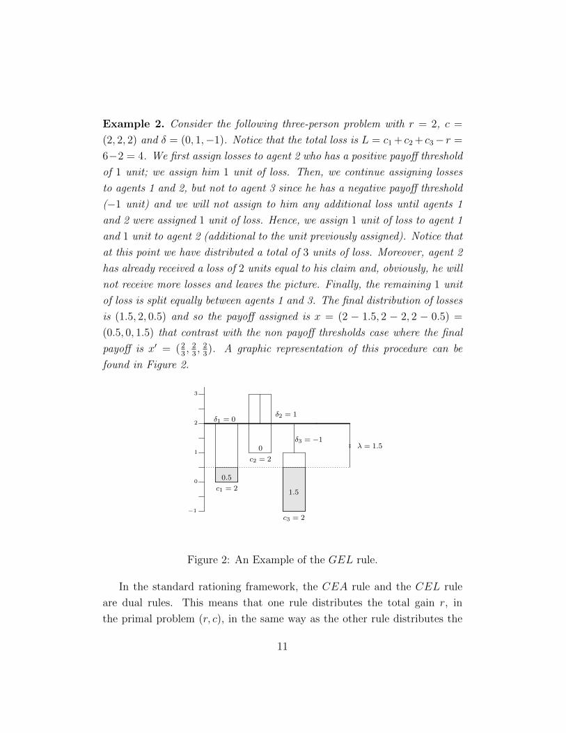
Example 2. Consider the following three-person problem with r = 2, c =
(2, 2, 2) and δ = (0, 1,−1). Notice that the total loss is L = c1 + c2 + c3− r =
6−2 = 4. We first assign losses to agent 2 who has a positive payoff threshold
of 1 unit; we assign him 1 unit of loss. Then, we continue assigning losses
to agents 1 and 2, but not to agent 3 since he has a negative payoff threshold
(−1 unit) and we will not assign to him any additional loss until agents 1
and 2 were assigned 1 unit of loss. Hence, we assign 1 unit of loss to agent 1
and 1 unit to agent 2 (additional to the unit previously assigned). Notice that
at this point we have distributed a total of 3 units of loss. Moreover, agent 2
has already received a loss of 2 units equal to his claim and, obviously, he will
not receive more losses and leaves the picture. Finally, the remaining 1 unit
of loss is split equally between agents 1 and 3. The final distribution of losses
is (1.5, 2, 0.5) and so the payoff assigned is x = (2 − 1.5, 2 − 2, 2 − 0.5) =
(0.5, 0, 1.5) that contrast with the non payoff thresholds case where the final
payoff is x′ = (23, 23, 23). A graphic representation of this procedure can be
found in Figure 2.
λ = 1.5
c1 = 2
2
1
0
0
−1
3
c2 = 2
c3 = 2
δ2 = 1δ1 = 0
δ3 = −1
0.5
1.5
0
Figure 2: An Example of the GEL rule.
In the standard rationing framework, the CEA rule and the CEL rule
are dual rules. This means that one rule distributes the total gain r, in
the primal problem (r, c), in the same way as the other rule distributes the
11

total loss L, where L =∑
i∈N ci − r, in the dual problem (L, c). The idea
of duality can be adapted for rationing problems with payoff thresholds but
taking into account that positive payoff thresholds become negative (and vice
versa) when passing from the primal problem (r, c, δ) to the dual problem
(L, c,−δ). Next we define formally dual rules.
Definition 7. F ∗ is the dual rule of F if, for all (r, c, δ) ∈ RN ,
F ∗(r, c, δ) = c− F (L, c,−δ).
The duality of the GEA and the GEL rule is maintained as it is the case
for the CEA and the CEL rule in the standard framework.
Proposition 2. The GEA and the GEL are dual rules from each other.
Proof. Let us first prove that GEA(r, c, δ) = c−GEL(L, c,−δ). By definition
and for all i ∈ N ,
GEAi(r, c, δ) = min{ci, (λ− δi)+}
= ci + min{0, (λ− δi)+ − ci}
= ci −max{0, ci − (λ− δi)+}.
(2)
By (2),∑
i∈N GEAi(r, c, δ) =∑
i∈N ci−∑
i∈N max{0, ci− (λ− δi)+} and
so∑
i∈N max{0, ci − (λ− δi)+} =∑
i∈N ci − r = L. Hence, max{0, ci − (λ−δi)+} = GELi(L, c,−δ) for all i ∈ N .
Next we prove that GEL(r, c, δ) = c − GEA(L, c, δ). By definition, for
all i ∈ N ,
GELi(r, c, δ) = max{0, ci − (λ+ δi)+}
= ci −min{ci, (λ+ δi)+}.(3)
By (3),∑
i∈N GELi(r, c, δ) =∑
i∈N ci −∑
i∈N min{ci, (λ+ δi)+} and so∑i∈N min{ci, (λ+ δi)+} =
∑i∈N ci − r = L.
Hence, min{ci, (λ + δi)+} = GEAi(L, c,−δ), for all i ∈ N . We conclude
that GEA and GEL are dual rules from each other.
�
12

3 Axiomatic characterizations
The CEA and the CEL rule (for standard rationing problems) had been
characterized by Herrero and Villar (2001) among others. Besides consistency
(a property that is common to most rationing rules) the properties that
characterize the CEA rule are path-independence and exemption. In this
section we will adapt the characterization to our framework.
First, to characterize the GEA rule we need the properties of path-
independence, consistency and we introduce a new property called compen-
sated exemption that can be viewed as an extension of the classical exemption
property for the two-person case.
Path-independence states that if we apply a rule to some problem (ob-
taining an allocation) but the available amount of resource diminishes sud-
denly, the new allocation obtained by applying again the rule (with the new
amount and the original claims) is equal to the one we would obtain using
the previous allocation as claims.
Property 1. A generalized rationing rule F satisfies path-independence if
for all (r, c, δ) ∈ RN and∑
i∈N ci ≥ r′ ≥ r it holds
F (r, c, δ) = F (r, F (r′, c, δ), δ).
If a rule satisfies path-independence it is monotonic with respect to the
available amount of resource as the reader may check. That is for all N , for
all c ∈ RN and for all r, r′ : {r ≤ r′ ≤∑
i∈N ci} ⇒ {F (r, c, δ) ≤ F (r′, c, δ)}.This property is called resource monotonicity.
Concerning exemption, this property requires that an agent with a small
enough claim will not suffer from rationing. In particular the two-person case
N = {i, j} states that if ci ≤ r2
then xi = ci.
Compensated exemption is defined just for the two-person case and re-
quires that exemption applies after payoff compensations between agents due
to differences in payoff thresholds are carried out. In case of δi > δj, this
property requires that if ci ≤ r−(δi−δj)2
then xi = ci. This property reads as
13
follows: we apply exemption taking into account not r but the net amount
after compensating agent j for the difference between payoff thresholds.
To cover the case where δi < δj, we define in general this property as
follows2:
Property 2. A generalized rationing rule F satisfies compensated exemption
if for any two-person rationing problem (r, c, δ) ∈ R{i,j} it holds that
if min{r, ci} ≤r − (δi − δj)
2=⇒ Fi(r, c, δ) = min{r, ci}.
On the other hand, consistency is a property that requires that if we
re-evaluate the allocation of resources within a subgroup of agents using the
same rule, the allocation does not change.
Property 3. A generalized rationing rule F is consistent if for all (r, c, δ) ∈RN and all T ⊆ N it holds
F (r, c, δ)|T = F
r − ∑i∈N\T
Fi(r, c, δ), c|T , δ|T
.
Next we show that the GEA rule satisfies these properties.
Proposition 3. The GEA rule satisfies path-independence.
Proof. Notice that if r = r′ the result is straightforward. Let us suppose now
that r < r′. We claim
GEA(r, c, δ) = GEA(r,GEA(r′, c, δ), δ).
Let i ∈ N ; by definition we have
GEAi(r, c, δ) = min{ci, (λ− δi)+} with∑
k∈N GEAk(r, c, δ) = r,
GEAi(r′, c, δ) = min{ci, (λ′ − δi)+} with
∑k∈N GEAk(r
′, c, δ) = r′ and
GEAi(r,GEA(r′, c, δ), δ) = min{min{ci, (λ′ − δi)+}, (λ′′ − δi)+}
with∑
k∈N GEAk(r,GEA(r′, c, δ), δ) = r.
2Notice that if δi = δj then compensated exemption implies exemption for two-person
case.
14

First, we claim
λ < λ′. (4)
If not, λ ≥ λ′, we would have that, for all i ∈ N ,
GEAi(r, c, δ) = min{ci, (λ− δi)+} ≥ min{ci, (λ′ − δi)+} = GEAi(r′, c, δ),
and adding up all the above inequalities, we obtain r =∑
i∈N GEAi(r, c, δ) ≥∑i∈N GEAi(r
′, c, δ) = r′ which contradicts r < r′.
Let us suppose now that GEA(r, c, δ) 6= GEA(r,GEA(r′, c, δ), δ) and so
there exists i∗ ∈ N such that
GEAi∗(r, c, δ) = min{ci∗ , (λ− δi∗)+}
< min{min{ci∗ , (λ′ − δi∗)+}, (λ′′ − δi∗)+}
= GEAi∗(r,GEA(r′, c, δ), δ) ≤ GEAi∗(r′, c, δ) ≤ ci∗ .
(5)
Hence, notice that min{ci∗ , (λ−δi∗)+} = (λ−δi∗)+. Taking this into account,
and substituting in (5), we have
(λ− δi∗)+ < min{min{ci∗ , (λ′ − δi∗)+}, (λ′′ − δi∗)+}
≤ (λ′′ − δi∗)+
and so we obtain that λ − δi∗ ≤ (λ − δi∗)+ < (λ′′ − δi∗)+ = λ′′ − δi∗ which
implies
λ < λ′′. (6)
Moreover, by (4) and (6) we get that, for all j ∈ N \ {i∗},
GEAj(r, c, δ) = min{cj, (λ− δj)+}
≤ min{cj,min{(λ′ − δj)+, (λ′′ − δj)+}}
= min{min{cj, (λ′ − δj)+}, (λ′′ − δj)+}
= GEAj(r,GEA(r′, c, δ), δ).
15

Finally, taking this into account, we conclude that
r =∑j∈N
GEAj(r, c, δ) = GEAi∗(r, c, δ) +∑
j∈N\{i∗}
GEAj(r, c, δ)
< GEAi∗(r,GEA(r′, c, δ), δ) +∑
j∈N\{i∗}
GEAj(r, c, δ)
≤∑j∈N
GEAj(r,GEA(r′, c, δ), δ) = r,
getting a contradiction. Therefore, we conclude
GEA(r, c, δ) = GEA(r,GEA(r′, c, δ), δ).
�
Proposition 4. The GEA rule satisfies compensated exemption.
Proof. Notice that if r = 0 the result is straightforward. Let (r, c, δ) ∈R{i,j} be a two-person rationing problem with payoff thresholds and let x∗ =
GEA(r, c, δ). Let us suppose to the contrary that (w.l.o.g.) min{r, ci} ≤r−(δi−δj)
2but x∗i < min{r, ci}. Hence, by efficiency, x∗j = r − x∗i > 0.
We consider two cases:
Case 1: r ≤ ci. In this case r ≤ r−(δi−δj)2
or
r + δi ≤ δj and so δj ≥ δi. (7)
Moreover, since x∗ = GEA(r, c, δ) and x∗i < ci, we claim x∗i = min{ci, (λ −δi)+} = (λ − δi)+ = λ − δi; otherwise 0 > λ − δi ≥ λ − δj, where the last
inequality follows from (7), and then x∗j = 0 which implies a contradiction.
On the other hand, since x∗ = GEA(r, c, δ) and x∗j > 0, we get 0 < x∗j =
min{cj, (λ − δj)+} = min{cj, λ − δj} ≤ λ − δj. However, if λ − δj > 0 we
would have that, by (7), λ > δj ≥ r + δi and so r < λ − δi = x∗i which is
infeasible.
Case 2: r > ci. In this case
ci ≤r − (δi − δj)
2. (8)
16
Since we are assuming that x∗i < ci < r and by definition of the GEA
rule, we get x∗i = min{ci, (λ − δi)+} = (λ − δi)+. If λ − δi ≥ 0 we have
r = x∗i + x∗j = λ− δi + x∗j ≤ λ− δi + λ− δj, where the last inequality follows
from 0 < x∗j = min{cj, (λ− δj)+} ≤ λ− δj. Henceforth r + δj ≤ 2λ− δi and
so, substituting in (8), ci ≤ λ − δi which implies that x∗i = ci contradicting
our hypothesis. On the other hand, if λ − δi < 0 we have that x∗i = 0
and r = x∗j ≤ λ − δj. Henceforth r + δj ≤ λ and so, substituting in (8),
ci ≤ λ−δi2
< 0 which is a contradiction.
We conclude that the GEA rule satisfies compensated exemption. �
Proposition 5. The GEA rule is consistent.
Proof. Notice that in Proposition 1 we characterize the GEA rule by making
payoff bilateral comparisons. Then, it is straightforward that if we reconsider
the problem within a subgroup of agents, then the solution must fulfill the
same bilateral comparisons and so the solution does not change.
�
The next theorem characterizes the GEA rule by means of the properties
we have presented.
Theorem 1. The GEA rule is the unique rule that satisfies path-independence,
compensated exemption and consistency.
Proof. TheGEA rule satisfies consistency (Proposition 5), path-independence
(Proposition 3) and compensated exemption (Proposition 4). Let us check
that it is unique. Let F be a rule satisfying these properties. If |N | = 1,
it is straightforward. Consider now the two-person case N = {1, 2} and
(r, c, δ) ∈ R{1,2}. Let us denote x∗ = (x∗1, x∗2) = F (r, c, δ). Let us suppose
that (w.l.o.g.) δ1 ≤ δ2. We consider three cases:
Case 1: r ≤ δ2 − δ1. Then,
min{r, c1} ≤ r =r
2+r
2≤ r − (δ1 − δ2)
2.
Hence, by compensated exemption, we have that x∗1 = min{r, c1} and x∗2 =
(r − c1)+ and so it is uniquely determined.
17

Case 2: r > δ2 − δ1 ≥ c1. Then,
min{r, c1} = c1 ≤ δ2 − δ1 =δ2 − δ1
2+δ2 − δ1
2<r − (δ1 − δ2)
2.
Hence, by compensated exemption, we have that x∗1 = min{r, c1} = c1 and
x∗2 = r − c1 and so it is uniquely determined.
Case 3: r > δ2 − δ1 and c1 > δ2 − δ1. We consider two subcases:
Subcase 3.a: c1 + δ1 = c2 + δ2. Since r > δ2 − δ1 and by Lemma 1 (see
Appendix) we have that x∗1 + δ1 = x∗2 + δ2 and so, taking into account that
x∗1 + x∗2 = r, it is uniquely determined.
Subcase 3.b: c1 + δ1 6= c2 + δ2. First, if for agent 1 min{r, c1} ≤ r−(δ1−δ2)2
,
then, by compensated exemption, x∗1 = min{r, c1} and x∗2 = (r − c1)+ and
so it is uniquely determined. Similarly for agent 2, if min{r, c2} ≤ r−(δ2−δ1)2
,
then, by compensated exemption, x∗2 = min{r, c2} and x∗1 = (r− c2)+ and so
it is uniquely determined. Otherwise,
min{r, ci}+ δi >r + δ1 + δ2
2for all i ∈ {1, 2}. (9)
Let us suppose that
ci + δi < cj + δj, where i, j ∈ {1, 2} with i 6= j. (10)
Now we claim that for r′ = 2ci + δi − δj, we have that x′ = F (r′, c, δ) is such
that x′i = ci and x′j = ci + δi − δj. To check it, first notice that, by (10),
r′ < ci + cj. Moreover, notice that ci + δi − δj ≥ 0; otherwise ci < δj − δiand if i = 1, we would get a contradiction with the hypothesis of Case 3,
and if i = 2, c2 < δ1 − δ2 ≤ 0 and we would reach a contradiction, where
the second inequality follows from the assumption δ1 ≤ δ2. Now, notice that
we can apply compensated exemption to the agent i in the problem (r′, c, δ),
since ci + δi − δj ≥ 0, and so
min{r′, ci}+ δi = min{2ci + δi − δj, ci}+ δi = ci + δi =r′ + δi + δj
2.
Hence, by compensated exemption, we have that x′i = ci. By efficiency,
x′j = r′ − x′i = ci + δi − δj, and the proof of the claim is done.
18

On the other hand, let us remark that r′ = 2ci + δi − δj ≥ 2 min{r, ci}+
δi − δj > r, where the last inequality follows from (9). Therefore, by path-
independence, we obtain
F (r, c, δ) = F (r, F (r′, c, δ), δ) = F (r, x′, δ).
Finally, notice that we can apply Lemma 1 to the problem (r, x′, δ) since
x′j + δj = ci + δi = x′i + δi and r > δ2 − δ1, where the inequality is the
hypothesis of Case 3. Then we get
Fi(r, c, δ) + δi = Fi(r, x′, δ) + δi = Fj(r, x
′, δ) + δj = Fj(r, c, δ) + δj,
where the first and the last equalities follow from path-independence and the
remainder equality follows from Lemma 1. Hence it is uniquely determined.
Then we conclude that, for the two-person case, the GEA rule is the unique
rule that satisfies path-independence and compensated exemption.
Let |N | ≥ 3 and suppose that F and F ′ satisfies the three properties
but F 6= F ′. Hence, there exists (r, c, δ) ∈ RN such that x = F (r, c, δ) 6=F ′(r, c, δ) = x′. This means that there exists i, j ∈ N such that xi > x′i,
xj < x′j and xi + xj ≤ x′i + x′j. However, since F and F ′ are consistent,
(xi, xj) = F (r −∑
k∈N\{i,j} xk, (ci, cj), (δi, δj)) and
(x′i, x′j) = F ′(r −
∑k∈N\{i,j} x
′k, (ci, cj), (δi, δj)).
Since path-independence implies resource monotonicity (see page 13) and
F = F ′ for the two-person case, we have that
(x′i, x′j) = F ′(x′i + x′j, (ci, cj)(δi, δj)) = F (x′i + x′j, (ci, cj)(δi, δj))
≥ F (xi + xj, (ci, cj)(δi, δj)) = (xi, xj).
Hence we reach a contradiction with xi > x′i. We conclude that the rule is
unique and F = GEA.
�
The properties that characterize the GEA rule are independent as the
reader may check in Examples 3, 4 and 5 in the Appendix.
19

In what follows, we characterize the GEL rule using the fact that the
GEA and GEL are dual rules (see Proposition 2). The properties that
characterize the GEL rule are the corresponding dual ones that characterize
the GEA rule.
Definition 8. P∗ is the dual property of P if for every rule F it is true that
F satisfies P if and only if its dual rule F ∗ satisfies P∗.
The dual property of compensated exemption is compensated exclusion
(see Proposition 6 in Appendix).
Property 4. A generalized rationing rule F satisfies compensated exclusion
if for any two-person rationing problem (r, c, δ) ∈ R{i,j} it holds that
if min{L, ci} ≤L− (δj − δi)
2=⇒ Fi(r, c, δ) = (r − cj)+.
Parallel to standard rationing problems (without payoff thresholds), the
dual property of path-independence is composition (see Proposition 7 in Ap-
pendix).
Property 5. A generalized rationing rule F satisfies composition if for all
(r, c, δ) ∈ RN and all r1, r2 ∈ R+ such that r1 + r2 = r, it holds
F (r, c, δ) = F (r1, c, δ) + F (r2, c− F (r1, c, δ), δ).
Before giving the characterization result for the GEL rule, let us men-
tion that Herrero and Villar connect the properties that characterize a rule
for a standard rationing problem with the properties that characterize the
corresponding dual rule.
“Theorem 0 (Herrero and Villar, 2001). If a rule F is character-
ized by a set of independent properties P = {P1,P2, . . . ,Pk} and
if for any Pi there exists a dual property P∗i , then the dual rule
F ∗ is characterized by the corresponding set of dual properties
P∗ = {P∗1 ,P∗2 , . . . ,P∗k}. Moreover, the properties in P∗ are also
independent”.
20

This result can be extended directly to the case of our generalized frame-
work. This allows to characterize the GEL rule by the corresponding dual
properties that characterize the GEA rule.
Theorem 2. The GEL rule is the unique rule that satisfies composition,
compensated exclusion and consistency.
Proof. We know that GEA and GEL are dual rules from each other (Propo-
sition 2). Moreover, compensated exclusion is the dual property of compen-
sated exemption (Proposition 6), composition is the dual property of path-
independence (Proposition 7) and consistency is dual of itself. Therefore, the
result follows from Theorem 0 of Herrero and Villar (2001). �
4 Conclusions
We have presented an extension of the standard model of rationing situations.
The aim of this extension is to take into account ex-ante inequalities of
agents (different from claims) involved in the rationing process and try to
compensate these inequalities. Two of the most outstanding rules (equal
awards and equal losses) have been generalized and characterized within this
new framework.
Two final remarks can be done as a future research work. Firstly, in
the standard rationing framework, there are two important solutions that we
have not analysed yet: the Talmudic rule and the proportional rule. With
respect to the Talmudic rule, notice that in the standard framework the
Talmudic is a self-dual rule and it is based essentially on the CEA and
the CEL rule. An extension to the case of rationing problems with payoff
thresholds and an analysis of self-duality might be interesting. With respect
to the proportional solution (another self-dual solution), it is not so clear
that the extension to the payoff thresholds framework should also maintain
the self-duality property.
Secondly, the consideration of payoff thresholds can be attributed not only
to priorities, past allocations or debts, but also to the fact that the same set of
21

agents might be involved in simultaneous or parallel rationing situations and
so we have to take into account what agents receive in a particular rationing
situation to distribute the resource in the remaining rationing situations. The
problem becomes not of a single-issue but of a multi-issue rationing nature.
A global approach to the overall rationing is needed. Payoff thresholds in
each particular single-issue rationing will not be exogenous to the model, but
endogenous in a global multi-issue rationing situation. The definition of rules
and extensions of the GEA rule and the GEL rule needs to be afforded.
References
[1] Aumann, R., & Maschler, M. (1985). Game theoretic analysis of a
bankruptcy problem from the Talmud. Journal of Economic Theory
36, 195-213.
[2] Herrero, C., & Villar, A. (2001). The three musketeers: four classical
solutions to bankruptcy problems. Mathematical Social Sciences 39,
307-328.
[3] Hougaard, J.L., Moreno-Ternero, J., & Østerdal, L.P. (2012). A unify-
ing framework for the problem of adjudicating conflicting claims. Jour-
nal of Mathematical Economics 48, 107-114.
[4] Hougaard, J.L., Moreno-Ternero, J., & Østerdal, L.P. (2013a). Ra-
tioning in the presence of baselines. Social Choice and Welfare 40,
1047-1066.
[5] Hougaard, J.L., Moreno-Ternero, J., & Østerdal, L.P. (2013b). Ra-
tioning with baselines: the composition extension operator. Annals of
Operations Research. DOI 10.1007/s10479-013-1471-8.
[6] Kaminski, M. (2000). Hydraulic rationing. Mathematical Social Sci-
ences 40, 131-155.
22

[7] Moulin, H. (2000). Priority rules and other asymmetric rationing meth-
ods. Econometrica 68, 643-684.
[8] O’Neill, B. (1982). A problem of rights arbitration from the Talmud.
Mathematical Social Sciences 2, 345-371.
[9] Pulido, M., Borm, P., Hendrickx, R., Llorca, N., & Sanchez-Soriano,
J. (2008). Compromise Solutions for Bankruptcy Situations with refer-
ences. Annals of Operations Research 158, 133-141.
[10] Pulido, M., Sanchez-Soriano, J. & Llorca, N. (2002). Game theory
techniques for university management: an extended bankruptcy model.
Annals of Operations Research 109, 129-142.
[11] Thomson, W. (2003). Axiomatic and game-theoretic analysis of
bankruptcy and taxation problems: a survey. Mathematical Social Sci-
ences 45, 249-297.
Appendix
Lemma 1. If a generalized rationing rule F satisfies compensated exemption
and path-independence then, for any (r, c, δ) ∈ R{1,2} it holds that
if c1 + δ1 = c2 + δ2 and r > |δ1 − δ2| =⇒ F1(r, c, δ) + δ1 = F2(r, c, δ) + δ2.
Proof. Let x∗ = F (r, c, δ). Consider c1 + δ1 = c2 + δ2 and r > |δ1 − δ2|, but
let us suppose to the contrary that (w.l.o.g.)
x∗1 + δ1 < x∗2 + δ2. (11)
By (11), notice that x∗1 + δ1 <x∗1+δ1+x
∗2+δ2
2= r+δ1+δ2
2and so x∗1 <
r+δ2−δ12
.
CLAIM. There exists r′ > r such that F1(r′, c, δ) = r+δ2−δ1
2.
Proof. Notice that r+δ2−δ12
> 0 since x∗1 ≥ 0. Notice also that r+δ2−δ12
≤ c1
since c1 + δ1 = c2 + δ2. Since F satisfies path-independence it also satisfies
resource monotonicity. Hence, F is a continuous and increasing function of r.
23

Therefore, by continuity, since F1(0, c, δ) = 0, F1(c1 + c2, c, δ) = c1 and F is
an increasing function in r, there will exist r′ such that F1(r′, c, δ) = r+δ2−δ1
2
and we are done. �Let us denote x′ = F (r′, c, δ). Notice that min{r, x′1} ≤ x′1 = r−(δ1−δ2)
2
which implies, by compensated exemption applied to the problem (r, x′, δ),
that F1(r, x′, δ) = min{r, x′1} = min{r, r+δ2−δ1
2} = r+δ2−δ1
2, where the last
equality follows from r > |δ2 − δ1|. Finally, by path-independence, we obtain
F (r, c, δ) = F (r, F (r′, c, δ), δ) =
(r + δ2 − δ1
2,r + δ1 − δ2
2
)and we conclude that x∗1 + δ1 = r+δ1+δ2
2= x∗2 + δ2. �
Example 3. Let F be a generalized rationing rule such that, for all (r, c, δ),
F (r, c, δ) = GEA(r, c,~0
).
This rule satisfies consistency and path-independence but does not verify
compensated exemption.
Example 4. Let (r, c, δ) ∈ RN and let us denote by ci = min{r, ci} the
truncated claim of agent i ∈ N . Up to reordering of agents, there exist
k1, k2, . . . , km such that k1 + k2 + . . .+ km = n and
c1 + δ1 = c2 + δ2 = . . . = ck1 + δk1
< ck1+1 + δk1+1 = ck1+2 + δk1+2 = . . . = ck1+k2 + δk1+k2
< ck1+k2+1 + δk1+k2+1 = . . . = ck1+k2+k3 + δk1+k2+k3...
< ck1+...+km−1+1 + δk1+...+km−1+1 = . . . = ck1+...+km + δk1+...+km .
Notice we have grouped the agents in m groups according to the value ci +
δi, where this value is constant within groups and strictly increasing across
groups. Let us denote each group by N1 = {i ∈ N : 1 ≤ i ≤ k1} and
Nt = {i ∈ N : k1 + . . .+ kt−1 + 1 ≤ i ≤ k1 + . . .+ kt}, for all t ∈ {2, . . . ,m}.
24

Then, can define recursively an allocation rule by assigning payoffs to the
members of each group as follows.
Step 1 (group N1):
If∑
i∈N1ci ≥ r then xi = GEAi(r, c|N1 , δ|N1), for all i ∈ N1, and xi = 0,
otherwise. Stop.
If not,∑
i∈N1ci < r, we assign xi = ci, for all i ∈ N1 and we go to the
next step.
Step t (2 ≤ t ≤ m, groups N2 to Nm):
If∑i∈Nt
ci ≥ r −∑i∈Nj
j=1,...,t−1
ci then xi = GEAi
r − ∑i∈Nj
j=1,...,t−1
ci, c|Nt , δ|Nt
,
for all i ∈ Nt, and xi = 0, for all i ∈ Nk with k = t+ 1, t+ 2, . . . ,m. Stop.
If not,∑i∈Nt
ci < r −∑i∈Nj
j=1,...,t−1
ci, we assign xi = ci, for all i ∈ Nt and we
go to the next step.
This rule satisfies consistency and compensated exemption but does not
verify path-independence.
Example 5. Let |N | ≥ 3 and define N = N1 ∪ N2 = {1, 2, . . . , n}, where
N1 = {1, 2} and N2 = N \ N1. Let CN1 = c1 + c2, CN2 =∑
i∈N2ci, ∆N1 =
δ1+δ2, and ∆N2 =∑
i∈N2δi. Next, let us denote by z = (z1, z2) the allocation
obtained by applying the GEA rule to the two-subgroup problem; that is
z = (z1, z2) = GEA (r, (CN1 , CN2), (∆N1 ,∆N2)) .
Then, define the rule F as follows: if |N | ≤ 2, F (r, c, δ) = GEA(r, c, δ); if
|N | ≥ 3
Fi(r, c, δ) =
GEAi (z1, (c1, c2), (δ1, δ2)) if i ∈ N1,
GEAi (z2, (ci)i∈N2 , (δi)i∈N2) if i ∈ N2.
This rule F satisfies compensated exemption and path-independence but it
is not consistent.
25

Proposition 6. Compensated exemption and compensated exclusion are dual
properties.
Proof. Let (r, c, δ) ∈ R{1,2} be a two-person rationing problem with pay-
off thresholds and let us suppose that F and F ∗ are dual rules, that is
F ∗(r, c, δ) = c−F (L, c,−δ). Hence, we claim that if F satisfies compensated
exemption then F ∗ satisfies compensated exclusion. To check it, suppose
(w.l.o.g.) that for the problem (r, c, δ), we have
min{L, c1} ≤L− (δ2 − δ1)
2. (12)
Notice that (12) is the same condition that we use in the definition of com-
pensated exemption when we apply the rule F to the problem (L, c,−δ).Hence, since F satisfies compensated exemption and by (12), we have
F ∗1 (r, c, δ) = c1 − F1(L, c,−δ) = c1 −min{c1, L} = max{0, c1 − L}
= max{0, c1 − (c1 + c2 − r)} = (r − c2)+.
We conclude that F ∗ satisfies compensated exclusion.
Similarly, we claim that if F satisfies compensated exclusion then F ∗
satisfies compensated exemption. Let us suppose (w.l.o.g.) that for the
problem (r, c, δ), we have
min{r, c1} ≤r − (δ1 − δ2)
2. (13)
Notice that (13) is the same condition that we use in the definition of compen-
sated exclusion when we apply the rule F to the problem (L, c,−δ). Hence,
since F satisfies compensated exclusion we have that
F ∗1 (r, c, δ) = c1 − F1(L, c,−δ) = c1 − (L− c2)+= c1 −max{0, L− c2} = min{c1, c1 + c2 − L}
= min{c1, r}.
We conclude that F ∗ satisfies compensated exemption.
�
26

Proposition 7. Path-independence and composition are dual properties.
Proof. Let us suppose that F and F ∗ are dual rules. Then, by definition
F ∗(r, c, δ) = c − F (L, c,−δ). We claim that if F satisfies composition then
F ∗ satisfies path-independence. To check it, let r ≥ r1 ≥ 0 and define
r2 = r − r1. Moreover, let L1 =∑
i∈N ci − r1. Hence,
L =∑i∈N
ci − r = L1 − r2, and so L1 ≥ L. (14)
On one hand, we have
F ∗(r1, c, δ) = c− F (L1, c,−δ)
= c− (F (L, c,−δ) + F (r2, c− F (L, c,−δ),−δ))
= F ∗(r, c, δ)− F (r2, c− F (L, c,−δ),−δ),
(15)
where the first and the last equality follows from definition of dual rule and
the second one follows from the composition property of F and (14).
On the other hand, by definition of dual rule, we have
F ∗(r1, F∗(r, c, δ), δ) = F ∗(r, c, δ)− F (r − r1, F ∗(r, c, δ),−δ)
= F ∗(r, c, δ)− F (r2, c− F (L, c,−δ),−δ).(16)
Therefore, since (15) and (16), F ∗ satisfies path-independence.
Similarly, we claim that if F satisfies path-independence then F ∗ satisfies
composition. To check it, let r1 + r2 = r, where r1, r2 ∈ R+ and L1 =∑i∈N ci − r1. Notice that L1 ≥ L. By path-independence and by definition
of dual rule, we have
F (L, c,−δ) = F (L, F (L1, c,−δ),−δ)
= F (L1, c,−δ)− F ∗(r2, F (L1, c,−δ), δ).(17)
Then, by definition of dual rule and by (17), we have
F ∗(r, c, δ) = c− F (L, c,−δ)
= c− (F (L1, c,−δ)− F ∗(r2, F (L1, c,−δ), δ))
= F ∗(r1, c, δ) + F ∗(r2, F (L1, c,−δ), δ)
= F ∗(r1, c, δ) + F ∗(r2, c− F ∗(r1, c, δ), δ).
27

Therefore F ∗ satisfies composition.
�
28