Rational Point Counts for del Pezzo Surfaces over Finite Fields and Coding Theory

A dissertation presented

by

Nathan Kaplan

to

The Department of Mathematics

in partial fulfillment of the requirementsfor the degree of

Doctor of Philosophyin the subject of

Mathematics

Harvard UniversityCambridge, Massachusetts

April 2013

© 2013 – Nathan KaplanAll rights reserved.

Dissertation Advisor: Professor Noam Elkies Nathan Kaplan

Rational Point Counts for del Pezzo Surfaces over Finite Fields and Coding Theory

Abstract

The goal of this thesis is to apply an approach due to Elkies to study the dis-

tribution of rational point counts for certain families of curves and surfaces over

finite fields. A vector space of polynomials over a fixed finite field Fq gives rise to

a linear code, and the weight enumerator of this code gives information about point

count distributions. The MacWilliams theorem gives a relation between the weight

enumerator of a linear code and the weight enumerator of its dual code.

For certain codes C coming from families of varieties where it is not known how to

determine the distribution of point counts directly, we analyze low-weight codewords

of the dual code and apply the MacWilliams theorem and its generalizations to gain

information about the weight enumerator of C. These low-weight dual codes can be

described in terms of point sets that fail to impose independent conditions on this

family of varieties.

Our main results concern rational point count distributions for del Pezzo surfaces

of degree 2, and for certain families of genus 1 curves. These weight enumerators

have interesting geometric and coding theoretic applications for small q.

iii

Contents

Acknowledgements vi

Chapter 1. Introduction 1

Chapter 2. Del Pezzo Surfaces over Finite Fields 14

1. The Geometry of del Pezzo Surfaces 14

2. The Picard Group of a Weak del Pezzo Surface 21

3. Points on del Pezzo Surfaces over Finite Fields 30

4. Point Counts for Cubic Surfaces 34

5. Codes from Degree 2 del Pezzo Surfaces 39

Chapter 3. Quadratic Residue Weight Enumerators and Elliptic Curves over

Finite Fields 47

1. The MacWilliams Theorem 47

2. MacWilliams Theorem for the Quadratic Residue Weight Enumerator 50

3. The Quadratic Residue Weight Enumerator for Quadrics 53

4. Cones over Singular Quartics on P1(Fq) 63

5. Elliptic Curves over Finite Fields and C1,4 68

6. The Quadratic Residue Weight Enumerator for Quartics on P1(Fq) 76

7. The Quadratic Residue Weight Enumerator of C⊥1,4 84

8. Quartic Curves with Non-Isolated Singularities 91

9. Other MacWilliams Theorems and Codes from Genus 1 Curves 100

Chapter 4. The Distribution of Point Counts for del Pezzo Surfaces of Degree 2105

1. A Sketch of the Proof 105

iv

2. Del Pezzo Surfaces of Trace 7 and 6 111

3. Examples of Surfaces of Maximal Trace for Small q 120

4. Dual Code Coefficients from del Pezzo Surfaces of Degree 2 136

Chapter 5. MacWilliams Identities for m-tuple Weight Enumerators 160

1. Statement of Results 161

2. The Proof of Theorem 102 167

3. Applications of Theorem 102 to Other Weight Enumerators 169

4. Support Weight Enumerators and Applications 171

5. The Repetition Code and the Parity Check Code 180

Chapter 6. Rational Points on Complete Intersections 184

1. Intersections of Two Conics in P2(Fq) 184

2. Del Pezzo Surfaces of Degree 4 188

3. (2, 2)-forms on P1(Fq)× P1(Fq) 191

4. Further Directions 197

Bibliography 200

v

Acknowledgements

I thank my advisor, Noam Elkies, for his guidance and support throughout this

project and his incredibly generosity with his time and his ideas. I also thank Henry

Cohn and Joe Harris for helpful discussions and for being valuable mentors through-

out my time in graduate school. Ramin Takloo-Bighash, Scott Chapman, and Joe

Gallian have also played important roles in my development during graduate school

and have given me great advice and encouragement.

I thank Nathan Pflueger and Ian Petrow for helpful discussions and comments

related to this project. I thank Alexander Barg, Thomas Britz, Irfan Siap, and two

anonymous referees for comments that helped improve Chapter 5. I thank Abhinav

Kumar for being a member of my thesis committee.

I thank Susan Gilbert and the rest of the staff of the Harvard math department

for all of the valuable work that they do to make the graduate program run smoothly.

I thank Robin Gottlieb and the preceptor staff for the thought and energy they put

into the teaching program. They have created a very positive environment to help

me and the other graduate students develop as educators.

I thank the NSF for supporting me with a Graduate Research Fellowship.

Finally, I thank my parents and Amie Sugarman for their support and encour-

agement.

vi

CHAPTER 1

Introduction

The main goal of this thesis is to apply an approach of Elkies using coding theory

to understand the distribution of rational point counts for a family of varieties over

a finite field [20]. In particular, we focus del Pezzo surfaces and certain families of

genus 1 curves. A vector space of polynomials gives a linear code, a linear subspace

of FNq for some N , and studying properties of this code will answer questions about

the distribution of rational point counts. The major coding theoretic tool that we

use is the relationship between a linear code C and its dual code C⊥, specifically

the relationship between their weight enumerators given by the MacWilliams theo-

rem. We prove several variations of the MacWilliams theorem that let us gain new

information about point counts.

We first state the problem in the language of algebraic geometry. Let V be a

variety over a finite field Fq and let L → V be a line bundle. We choose an M -

dimensional space C of sections of L. We also require that there is no nonzero

c ∈ C that vanishes on all of V (Fq). Then C gives a map ϕ : V (Fq) → PM−1(Fq).

As we vary over all c ∈ C, what is the distribution of the number of points of

p ∈ V (Fq) | c(p) = 0? We study C as a linear subspace of FNq where N = #V (Fq).

A linear subspace of FNq is also known as a linear code. For example we consider

V = Pn(Fq), L = O(d), and C = Γ(L) (homogeneous degree d polynomials on

Pn) and get a linear code over FNq where N = (qn+1 − 1)/(q − 1). In other parts

of this thesis V will not be a projective space but some other variety, for example

P1(Fq)× P1(Fq) or a smooth quadric in P4(Fq).

1

We now give some of the key definitions in coding theory that will play a major

role throughout this thesis.

Definition. A code C is a subset of FNq . We say that C is a linear code if C is a

linear subspace, that is, for all c1, c2 ∈ C we have c1 + c2 ∈ C and ac ∈ C for all

a ∈ Fq.

For x, y ∈ FNq define the Hamming distance d(x, y) as the number of coordinates

in which they differ. That is, if x = (x1, x2, . . . , xN) and y = (y1, y2, . . . , yN) then

d(x, y) = #i such that xi 6= yi, 1 ≤ i ≤ N.

For x ∈ FNq we define wt(x), the weight of x, to be d(x, 0), the number of nonzero

coordinates of x.

In this thesis we study codes coming from the evaluation of polynomials. Given

a polynomial f , the weight of the codeword associated to f gives the number of

zeros of the variety cut out by f . Our goal is to understand how these counts vary

as we consider all of the polynomials in a given vector space. Therefore, it will be

convenient to have a way to keep track of the distribution of weights that occur in a

code C.

Definition. The Hamming weight enumerator of a code C is a homogeneous poly-

nomial

WC(X, Y ) =∑c∈C

XN−wt(c)Y wt(c) =N∑i=0

AiXN−iY i,

where

Ai = #c ∈ C such that wt(c) = i.

This project builds heavily on work of Elkies [20] in which he determines the

Hamming weight enumerator for the code of homogeneous cubics in P3(Fq). In the

language of the paragraph above, this is the code with V = P3(Fq), L = O(3), and

2

C its space of global sections. More concretely, consider the q20 homogeneous cubic

polynomials f3(w, x, y, z) on P3(Fq), which has N := q3 + q2 + q + 1 points. It does

not really make sense to evaluate a polynomial at point of P3 since the coordinates of

such a point are defined only up to scalar multiplication, but whether a polynomial

evaluated at a point is zero or nonzero does not depend on the scalar multiple chosen.

By fixing an affine representative for each projective point and choosing some ordering

for these N points, evaluation now gives a well defined map taking a polynomial to

an element of FNq . Changing the choice of affine representatives gives an equivalent

code.

The goal is to determine for each t ∈ [0, N ], how many of these cubics have t

zeros. This is exactly the information contained in the Hamming weight enumerator

of C. The zeros of a cubic polynomial f3 are the Fq-points of the variety given by

f3(w, x, y, z) = 0, so this problem is equivalent to understanding the distribution of

the number of Fq-points for this family of varieties.

There is a dual code C⊥ associated to a linear code C ⊂ FNq , and studying

properties of this dual code often helps lead to a better understanding of C. We

being with some definitions.

Definition. Let x = (x1, . . . , xN) and y = (y1, . . . , yN) be two elements of FNq . Define

a pairing

〈·, ·〉 : FNq × FNq → FNq

by

〈x, y〉 :=N∑i=1

xiyi.

Given a linear code C we define the dual code

C⊥ := y ∈ FNq : ∀x ∈ C, 〈x, y〉 = 0.

3

Throughout this thesis we study a linear code C by studying properties of the

dual code C⊥. The MacWilliams theorem of coding theory allows us to draw con-

clusions about the weight enumerator of C given information about the weights of

codewords of C⊥. In fact, the weight enumerator of C completely determines the

weight enumerator of C⊥ and vice versa [33]. In Chapter 3 we give a proof of the

following theorem using discrete Poisson summation.

Theorem 1 (MacWilliams). Let C be a linear code over FNq . Then

WC⊥(X, Y ) =1

|C|WC(X + (q − 1)Y,X − Y ).

In order to determine the weight enumerator of a linear code C, it suffices to com-

pute the weight enumerator of C⊥. Since the codewords of C come from evaluating

polynomials, the codewords of the dual code C⊥ are also related to the geometry of

projective space. We define the support of a codeword c to be the set of points p in

Pn(Fq) such that the coordinate of c corresponding to p is nonzero. If C is a code that

comes from the evaluation of polynomials, then codewords of C⊥ have supports that

fail to impose independent conditions on these polynomials, that is, the dimension of

the space of polynomials vanishing at these points exceeds what we expect for gener-

ically chosen points. With the description given above, points imposing dependent

conditions are subsets S ⊂ Pn(Fq) for which ϕ(S) is linearly dependent.

This is the subject of interpolation problems in algebraic geometry: given a vari-

ety V and a vector space of polynomials, describe all configurations of n points of V

that fail to impose independent conditions on these polynomials. It is often easier to

count point sets failing to impose independent conditions than it is to count ratio-

nal points on varieties directly. This gives information about the possible supports

of dual codewords, and the MacWilliams theorem lets us draw conclusions about

distributions of rational point counts.

4

We give an example from [20] to motivate this kind of analysis. We denote the

code of homogeneous degree d forms on Pn(Fq) by Cn,d. Consider the code Cn,1 of

linear forms on Pn(Fq). Linear forms give an n + 1 dimensional vector space, and

evaluation gives a map to FNq where N = (qn+1 − 1)/(q − 1). Every nonzero linear

form defines a hyperplane in Pn(Fq) that has (qn − 1)/(q − 1) Fq-rational points.

Therefore the weight enumerator of this code is given by

WCn,1(X, Y ) = XN + (qn+1 − 1)XN−qnY qn .

Applying the MacWilliams theorem shows that

WC⊥n,1(X, Y ) = XN +

(qn+1 − 1)(qn − 1)q

6XN−3Y 3 +O(Y 4).

We see that the number of weight 3 codewords of the dual code is exactly q−1 times

the number of triples of collinear points in Pn(Fq). It is not difficult to check that

every collinear triple occurs as the support of exactly q−1 codewords, and that these

are the only possible supports.

We explain in more detail how the supports of dual codewords relate to points

that fail to impose independent conditions in the case of linear forms on P2(Fq).

Suppose we have c ∈ C⊥2,1 of weight three. There are three nonzero coordinates of

c, ai, aj, ak, and each coordinate corresponds to a point in P2(Fq). We have

aif(pi) + ajf(pj) + akf(pk) = 0,

for all linear forms f(x, y, z). Since aif(pi) + ajf(pj) = −akf(pk), the value of f(pk)

can be determined from the value of f(pi) and f(pj). In particular, it is not possible

for f(x, y, z) to vanish on the points pi and pj, but be nonzero at pk. Therefore, these

points are collinear. They fail to impose independent conditions on linear forms

because we do not expect any linear form to vanish on three generic points, but for

collinear points such a form does exist.

5

A dual codeword carries more information than just the fact that the support

corresponds to points failing to impose independent conditions. It explicitly gives

a linear relation among values of these functions taken at these points. Suppose

p1, . . . , p4 are four points of a line L ⊂ P2(Fq) and p5 is a point not on L. Bezout’s

theorem implies that a conic intersecting a line at 4 points must contain that line.

Generically, given five points there is a unique conic containing them, but here we

have all conics consisting of L together with a line through p5. So, these points fail

to impose independent conditions on degree 2 polynomials in P2(Fq).

Suppose we have a dual codeword c with support p1, . . . , p5. For concreteness we

suppose that L is given by the line z = 0 and p5 = (0, 0, 1), the affine representative

of [0 : 0 : 1]. The nonzero coordinates of c are coefficients ai satisfying

5∑i=1

aif(pi) = a5f(p5) +4∑i=1

aif(pi) = 0, for all

f(x, y, z) = b1x2 + b2xy + b3xz + b4y

2 + b5yz + b6z2.

This implies

a5b6 +4∑i=1

aif(pi) = 0.

The terms f(pi) for each i satisfying 1 ≤ i ≤ 4 are linear combinations of the

coefficients b1, b2, and b4. The only way for this equality to hold for all f(x, y, z) is

for a5 = 0. These points fail to impose independent conditions, so we can find dual

codewords supported on them. We have seen that every linear relation supported on

these points has a5 = 0. Throughout this thesis we will be interested in counting

dual codewords of given weight, and will need to do more than just determine the

point sets failing to impose independent conditions.

The family of codes arising from evaluation of polynomials contains some famous

examples from coding theory. This code of linear forms on Pn(Fq) is the q-ary Simplex

Code of dimension n + 1, an interesting object that arises in other areas of coding

6

theory and has other constructions [26]. Its dual is the more famous q-ary Hamming

code, one of the most studied objects in coding theory. This construction of these

famous codes in terms of linear forms on Pn(Fq) lets us study them using the geometry

of Pn(Fq).

A common theme of this thesis will be the use of refinements of the classical

Hamming weight enumerator that keep track of more information about a code to

draw conclusions about rational points. We give such an example in the setting of

linear forms on P2(Fq).

Definition. We define the 2-tuple weight enumerator of a code C ⊆ FNq by

W[2]C (X, Y ) =

N∑i=0

BiXN−iY i,

where Bi is equal to the number of pairs of codewords x, y ∈ C with x = (x1, . . . , xN)

and y = (y1, . . . , yN) such that there are N − i coordinates for which xj = yj = 0.

This weight enumerator tells us about the common zeros among pairs of code-

words drawn from the same code. If a code C comes from the evaluation of some

vector space of polynomials, then its 2-tuple weight enumerator gives information

about the distribution of counts for common zeros of pairs of polynomials in this

space. This tells us about the counts for rational points on complete intersections of

codimension 2.

As a first example, consider the code C2,1 of linear forms on P2(Fq). We have

already seen that

WC2,1(X, Y ) = Xq2+q+1 + (q3 − 1)Xq+1Y q2 .

A simple calculation gives the 2-tuple weight enumerator

W[2]C2,1

(X, Y ) = Xq2+q+1 + (q2 − 1)(q2 + q + 1)Xq+1Y q2 + (q − 1)2(q2 + q + 1)XY q2+q,

7

since any pair of distinct Fq-rational lines intersect in a unique point of P2(Fq).

The MacWilliams theorem extends to this 2-tuple weight enumerator and to other

generalizations. In Chapter 5 we will develop the theory of these higher weight

enumerators, and in Chapter 6 we will use them to study certain codes coming from

varieties.

Proposition 2. Let C be a linear code over FNq . Then

W[2]

C⊥(X, Y ) =

1

|C|2W

[2]C (X + (q2 − 1)Y,X − Y ).

In this particular case, we see that

W[2]

C⊥2,1(X, Y ) − (q + 1)(WC⊥2,1

(X, Y )−Xq2+q+1)−Xq2+q+1

=(q − 2)(q − 1)3q2(q + 1)2(q2 + q + 1)

24Xq2+q−2Y 3 +O(Y 4).

This is (q − 1)2q(q + 1) times the number of collections of four collinear points in

P2(Fq), the number of choices of a basis for a 2-dimensional subspace of C⊥2,1 that is

spanned by two codewords of weight three such that the union of their supports is

four collinear points. We will explain this type of result in further detail in Chapter 6.

The Hamming weight enumerator keeps track only of the number of coordinates of

a codeword that are zero and the number that are nonzero. All nonzero coordinates

are treated the same. Much of this thesis is focused on counting points on varieties

expressed as double covers of P1 and of P2, so it will be useful to distinguish between

coordinates that are nonzero squares in F∗q and coordinates that are non-squares of

F∗q.

Definition. For a field Fq of characteristic not equal to 2, let r(q) denote the set of

squares in F∗q and s(q) denote the set of non-squares in F∗q. For x = (x1, . . . , xN) ∈ Fq8

we define

Res(x) = #i such that xi ∈ r(q), and NRes(x) = #i such that xi ∈ s(q).

We see that Res(x) + NRes(x) = wt(x).

Given a linear code C ⊂ FNq we define the quadratic residue weight enumerator

of C to be the homogeneous polynomial in three variables defined by

QRC(X, Y, Z) =∑c∈C

XN−wt(c)Y Res(c)ZNRes(c).

We first give an example of an application of this weight enumerator. Consider

homogeneous quadratic polynomials on P1(Fq), binary quadratic forms, C1,2. It is a

simple exercise to write down the weight enumerator of this three-dimensional code:

WC1,2(X, Y ) = Xq+1 +(q + 1)q(q − 1)

2X2Y q−1 + (q− 1)(q+ 1)XY q +

(q − 1)2q

2Y q+1.

Suppose we are interested in knowing the distribution of point counts for w2 = f2(x, y)

as f2(x, y) varies over all homogeneous quadratic polynomials. This is equivalent to

knowing QRC1,2(X,X2, 1). In this case the quadratic residue weight enumerator is

not difficult to determine, as each such variety defines a conic in P2(Fq). There are

two types of points on this variety, those that come from w = 0 and f2(x, y) = 0, and

pairs of points coming from points for which f2(x, y) is a nonzero square. We can

gain extra information by keeping track of these counts separately.

We note that any quadratic polynomial f2(x, y) on P1(Fq) with two distinct roots

defines a variety w2 = f2(x, y) in P2(Fq) that is a smooth conic. This does not

depend on whether the two roots are Fq-rational or a pair of Galois-conjugate points

defined over Fq2 . All smooth conics are equivalent under automorphisms of P2(Fq)

and in particular, have q + 1 Fq-rational points. If f2(x, y) has a double zero, then

w2 = f2(x, y) gives the intersection of two lines. For a fixed f2(x, y), half of the

scalar multiples of the right hand side of this equation give the intersection of two

9

Fq-rational lines and half give the intersection of two Galois-conjugate lines. This

shows that the quadratic residue weight enumerator is given by

QRC1,2(X, Y, Z) = Xq+1 +

(q + 1)q(q − 1)

2X2Y

q−12 Z

q−12

+(q − 1)(q + 1)

2X(Y q + Zq) +

(q − 1)2q

2Y

q+12 Z

q+12 .

The minimum weight codewords of C1,2⊥ have weight 4 and the MacWilliams theorem

for this enumerator shows how these four nonzero coordinates split up into nonzero

squares and non-squares. In this case, the (q − 1)(q+1

4

)dual codewords of weight 4

contribute

(q − 1)3q(q + 1)

32Y 2Z2 +

(q − 5)(q − 1)2q(q + 1)

192

(Y 4 + Z4

),

to the quadratic residue weight enumerator of C1,2⊥ if q ≡ 1 (mod 4) and contribute

(q − 3)(q − 1)2q(q + 1)

32Y 2Z2 +

(q − 1)2q(q + 1)2

192

(Y 4 + Z4

),

if q ≡ 3 (mod 4).

We give the quadratic residue weight enumerator for the code of quadrics in

Pn(Fq), QRCn,2(X, Y, Z), in Chapter 3. We also apply the MacWilliams theorem for

this weight enumerator to get information about the low-weight dual code coefficients.

We compute this quadratic residue weight enumerator for quartics on P1(Fq) in

Chapter 3 and use it to analyze points on families of elliptic curves over finite fields.

We will give a more refined version of a result of Schoof [40] that builds on work of

Deuring and Waterhouse [14, 52]. Applying the MacWilliams theorem here leads to

interesting questions about powers of traces of elliptic curves over finite fields that

are related to previous results of Birch [3].

The largest part of this thesis is spent studying del Pezzo surfaces of degree 2

over finite fields. In Chapter 2 we will review the theory of del Pezzo surfaces over

10

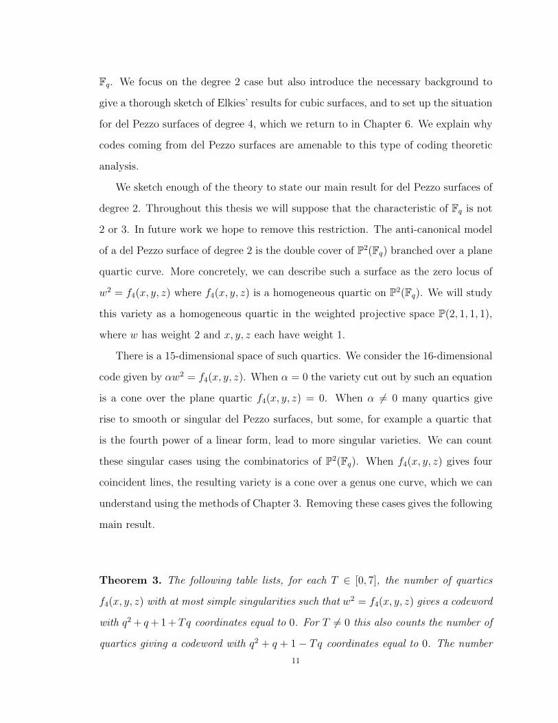
Fq. We focus on the degree 2 case but also introduce the necessary background to

give a thorough sketch of Elkies’ results for cubic surfaces, and to set up the situation

for del Pezzo surfaces of degree 4, which we return to in Chapter 6. We explain why

codes coming from del Pezzo surfaces are amenable to this type of coding theoretic

analysis.

We sketch enough of the theory to state our main result for del Pezzo surfaces of

degree 2. Throughout this thesis we will suppose that the characteristic of Fq is not

2 or 3. In future work we hope to remove this restriction. The anti-canonical model

of a del Pezzo surface of degree 2 is the double cover of P2(Fq) branched over a plane

quartic curve. More concretely, we can describe such a surface as the zero locus of

w2 = f4(x, y, z) where f4(x, y, z) is a homogeneous quartic on P2(Fq). We will study

this variety as a homogeneous quartic in the weighted projective space P(2, 1, 1, 1),

where w has weight 2 and x, y, z each have weight 1.

There is a 15-dimensional space of such quartics. We consider the 16-dimensional

code given by αw2 = f4(x, y, z). When α = 0 the variety cut out by such an equation

is a cone over the plane quartic f4(x, y, z) = 0. When α 6= 0 many quartics give

rise to smooth or singular del Pezzo surfaces, but some, for example a quartic that

is the fourth power of a linear form, lead to more singular varieties. We can count

these singular cases using the combinatorics of P2(Fq). When f4(x, y, z) gives four

coincident lines, the resulting variety is a cone over a genus one curve, which we can

understand using the methods of Chapter 3. Removing these cases gives the following

main result.

Theorem 3. The following table lists, for each T ∈ [0, 7], the number of quartics

f4(x, y, z) with at most simple singularities such that w2 = f4(x, y, z) gives a codeword

with q2 + q+ 1 +Tq coordinates equal to 0. For T 6= 0 this also counts the number of

quartics giving a codeword with q2 + q + 1− Tq coordinates equal to 0. The number

11

is given as a multiple of |GL3(Fq)|/2903040.

T 2903040/|GL3(Fq)| times the number of w2 = f4(x, y, z) of weight q3 − Tq − 1

0 26·33·653|GL3(Fq)|

(q15 + 4103

15672q14 − 18773

15672q13 + 10715

3918q12 − 32417

7836q11 + 173425

15672q10 − 274399

15672q9

+13229915672

q8 + 4440715672

q7 − 81673918

q6 − 1302653

q5 − 663535224

q4 + 828455224

q3 − 1680653

q2 + 1680653

)1 3·7·29·1187

(q−1)(q+1)

(q8 + 24499

34423q7 + 67671

34423q6 + 10890

34423q5

+21361234423

q4 − 32454934423

q3 + 50039934423

q2 + 35828034423

q − 60874534423

)2 27 · 7 · 132

(q6 + 15415

10816q5 + 1025

1352q4 + 77035

10816q3 − 198671

10816q2 + 314675

5408q − 653745

10816

)3 33 · 5 · 7 · 13

(q6 + 31

39q5 + 70

13q4 − 1591

39q3 + 2446

13q2 − 6536

13q + 6351

13

)4 25 · 3 · 7

(q6 + 5

8q5 − 185

4q4 + 3095

8q3 − 15673

8q2 + 9695

2q − 34965

8

)5 32 · 7(q − 3) (q5 − 12q4 + 146q3 − 1235q2 + 4461q − 5185)

6 2 · 32 · 7(q − 7)(q − 5)(q − 3)(q2 − 9q + 15)

7 (q − 7)(q − 5)(q − 3)(q3 − 20q2 + 119q − 175)

This is the analogue of a result of Elkies for cubic surfaces [20]. This theorem has

some interesting geometric consequences for small q. For example, for q = 9, 11, there

is a unique del Pezzo surface with q2 + 8q+ 1 Fq-rational points up to automorphism,

while for q = 13 there are two isomorphism classes of such surfaces. We also show

that for q satisfying certain congruence conditions w2 = x4 +y4 +z4 gives a del Pezzo

surface with the maximal number of rational points. We prove this theorem and

discuss these types of consequences in Chapter 4.

This approach has the potential to be applied in several other settings. For

example, in Chapter 6 we set up much of the necessary material to prove the analogue

of this result for del Pezzo surfaces of degree 4.

We note that his project fits in with previous work on counting points on varieties

over finite fields. For example, Li has studied del Pezzo surfaces of degree 1 and 2 that

have few rational points over Fq for small q [31]. Codes from del Pezzo surfaces have

12

also been investigated by Tsfasman and Vladut [49], and Boguslavsky [4, 5], although

their work focuses more on finding the minimal weights of subcodes rather than

determining weight enumerators. More generally, codes coming from the evaluation

of polynomials include famous examples such as Goppa codes and Reed-Solomon

codes. Codes coming from quadrics and from curves given as complete intersections

have been studied previously, but again, the focus has been on determining minimal

weights rather than weight enumerators [46, 47, 50, 51]. Finally, low-weight dual

codewords of codes of this type have been studied by Couvreur [13], and Fontanari

and Marcolla [22].

There is a large computational component to this thesis. Most of these computa-

tions were done in the computer algebra system Sage [45]. We also use the algebra

system Magma in Chapter 4 to compute the automorphism groups of certain curves

over finite fields [6].

13

CHAPTER 2

Del Pezzo Surfaces over Finite Fields

This chapter gives the necessary background for the weight enumerator calculation

for del Pezzo surfaces of degree 2. We begin by giving several of the basic definitions

in this area and reviewing the classical theory. We will also give a fairly detailed

sketch of Elkies’ results about the distribution of point counts for cubic surfaces [20].

At the end of this chapter we give an outline of the proof of Theorem 3, breaking it up

into a combinatorial part, a part about elliptic curves over finite fields, and a rather

intricate computation involving low-weight coefficients of the dual of two particular

codes.

We will state a first goal for this section.

Proposition 4. Suppose that f4(x, y, z) = 0 defines a plane quartic that does not

have non-isolated singularities and is not the union of four coincident lines. Then

w2 = f4(x, y, z) defines a homogeneous quartic in P(2, 1, 1, 1) with q2 + q+ 1 + tq Fq-

rational points, for some integer t ∈ [−7, 7].

1. The Geometry of del Pezzo Surfaces

This section relies heavily on Chapter 8 of Dolgachev’s book [15]. We begin with

the classical definition of a del Pezzo surface. We recall that a surface in Pn is called

nondegenerate if it is not contained in a proper linear subspace of Pn.

Definition. A del Pezzo surface is a nondegenerate irreducible surface of degree d in

Pd that is not a cone and not isomorphic to a projection of a surface of degree d in

Pd+1.

14

The more modern viewpoint is to define these surfaces in terms of the anti-

canonical class −KS.

Definition. A del Pezzo surface is a nonsingular surface S with ample −KS. A

weak del Pezzo surface is a nonsingular surface with −KS nef and big.

We recall that a divisor D is called nef, or numerically effective, if for any irre-

ducible curve C the intersection number C ·D > 0. If we only require C ·D ≥ 0 then

D is called ample. We say that D is big if its self-intersection is positive, D2 > 0.

We will refer to a singular surface that has minimal desingularization equal to a

del Pezzo surface as a singular del Pezzo surface. The most natural invariant of a del

Pezzo surface is its degree.

Definition. The number d := K2S is called the degree of a weak del Pezzo surface.

It is not difficult to prove that a del Pezzo surface has degree at most 9. In this

thesis we focus on the particular case of del Pezzo surfaces of degree 2, but also discuss

Elkies’ work on del Pezzo surfaces of degree 3 (cubic surfaces) and will mention del

Pezzo surfaces of degree 4 in Chapter 6. Del Pezzo surfaces of different degrees have

much in common, but each degree has its own flavor.

The definition of a weak del Pezzo surface limits the types of curves it can contain.

The curves that do appear play a special role in the study of rational points of del

Pezzo surfaces over finite fields.

Proposition 5. Let S be a weak del Pezzo surface. Then any irreducible reduced

curve C on S with negative self-intersection satisfies C · C = −1 or −2.

This is Lemma 8.1.13 of [15]. We say that such a C is a (−1)-curve, or a (−2)-

curve, respectively. The divisor classes of these curves play an important role in

studying the Picard group Pic(S) of S, because they arise from blow-ups.

15

Del Pezzo surfaces have only rational double points as singularities. These singu-

larities are related to the presence of (−2)-curves on the minimal desingularization

of the surface. We will not need to study these singularities in detail. For more

information see [15].

Proposition 6.

(1) A del Pezzo surface S has only rational double points as singularities.

(2) A smooth del Pezzo surface S does not contain any (−2)-curves. Let S be

a singular del Pezzo surface and π : S → S a minimal desingularization.

Then S is a weak del Pezzo surface and the inverse image of the singular

points of S is exactly the collection of (−2)-curves on S.

The first part of this statement is Theorem 8.1.11 in [15]. The second part follows

from Theorem 2.4.4 of [32].

We see that S has a rational double point if and only if its minimal desingulariza-

tion S has a (−2)-curve. We are primarily concerned with rational points not on del

Pezzo surfaces S, but on the anti-canonical model of S, which we define below. For

example, we do not study rational points on del Pezzo surfaces of degree 3, but on

models of such surfaces as cubic hypersurfaces in P3(Fq), and do not study points on

del Pezzo surfaces of degree 2, but on double covers of P2(Fq) branched over a plane

quartic. The rational double points on S, the (−2)-curves on S, and singular points

on these models, for example on the cubic surface or quartic curve, are all closely

related.

We would like to give a concrete way to produce all del Pezzo surfaces of given

degree d over a fixed finite field Fq. We can do this by describing these surfaces as

the blow-up of P2 at 9− d points. We first recall that a blow-up of a variety X at a

point x is a variety X along with a morphism π : X → X. The inverse image of x

is called the exceptional divisor E of the blow-up, and π is an isomorphism outside

16

of E. A point x′ ∈ X is infinitely near to x if it lies in the support of E. Given a

collection of points x1, . . . , xn, the point xi is proper if no xj with j 6= i is infinitely

near to xi.

For the blow-up P2 atN points, we consider a composition of birational morphisms

π : S = Skπk→ Sk−1

πk−1−→ · · · π2→ S1π1→ P2,

where each πi : Si → Si−1 is the blow-up of a point xi in Si−1. If all of these points

are proper, then they are in P2, but can also consider the blow-up of P2 at infinitely

near points.

We note that F2 is the Hirzebruch surface, a minimal ruled surface. The following

result is Corollary 8.1.17 of [15].

Theorem 7. Let S be a weak del Pezzo surface. Then either S ∼= P1×P1, or S ∼= F2,

or S is obtained from P2 by blowing up N ≤ 8 points. If S is a nonsingular del Pezzo

surface, then the case S ∼= F2 does not occur.

It is not the case that blowing up any collection of N ≤ 8 points leads to a weak

del Pezzo surface. We give exactly the conditions that yield weak del Pezzo surfaces.

Proposition 8. Let η = x1, . . . , xr be a collection of points in P2, possibly infinitely

near, and Sη be the blow-up of these points. Then Sη is a weak del Pezzo surface if

and only if each of the following conditions holds:

(1) r ≤ 8;

(2) the Enriques diagram of η is the disjoint union of chains;

(3) |OP2(1)− η′| = ∅ for any η′ ⊂ η consisting of four points;

(4) |OP2(2)− η′| = ∅ for any η′ ⊂ η consisting of seven points.

This is Corollary 8.1.24 of [15]. We will not define the Enriques diagram here

because it is not needed in what follows. See Section 7.3.2 of [15] for details.

17

Points satisfying these four conditions are said to be in almost general position.

We next give the analogous definition for general position and the analogue of the

above result for del Pezzo surfaces.

Definition. We say that a collection of points is in general position if each of the

following conditions holds:

(1) all points are proper points;

(2) no three points are on a line;

(3) no six points are on a conic.

Proposition 9. The blow-up of N ≤ 7 points in P2 is a smooth del Pezzo surface if

and only if the points are in general position.

The blow-up of 8 points in P2 is a smooth del Pezzo surface if and only if it

satisfies these conditions and also no cubic passes through these 8 points with one of

the points being a singular point.

The first part of this result follows from Proposition 8. The second part is Propo-

sition 8.1.25 of [15].

Next we describe how this modern notion of del Pezzo surface relates to the classi-

cal definition that began this section. This connection comes from the anti-canonical

map. The following result, Theorem 8.3.2 of [15], explains why we study the particu-

lar models of curves mentioned above, cubic surfaces and double covers of P2 branched

over plane quartics. This also provides a concrete link between rational double points

of a del Pezzo surface and the (−2)-curves of its minimal desingularization.

Theorem 10. Let S be a weak del Pezzo surface of degree d and let R be the union

of (−2)-curves on S. Then we have the following:

(1) |−KS| has no fixed part.

(2) If d > 1, then |−KS| has no base points.

18

(3) If d > 2, then |−KS| defines a regular map φ to Pd that is an isomorphism

outside of R. The image surface S is a del Pezzo surface of degree d in Pd.

The image of each connected component of R is a rational double point of

φ(S).

(4) If d = 2, then |−KS| defines a regular map φ : S → P2. It factors as a

birational morphism f : S → S onto a normal surface and a finite map

π : S → P2 of degree 2 branched along a not necessarily irreducible curve

B of degree 4. The image of each connected component of R is a rational

double point of S. The curve B is either nonsingular or has only simple

singularities.

(5) If d = 1, then |−2KS| defines a regular map φ : S → P3. It factors as a

birational morphism f : S → S onto a normal surface and a finite map

π : S → Q ⊂ P3 of degree 2, where Q is a quadric cone. The morphism π is

branched along a curve B of degree 6 cut out on Q by a cubic surface. The

image of each connected component of R under f is a rational double point

of S. The curve B is either nonsingular or has only simple singularities.

We emphasize a certain difficulty in studying del Pezzo surfaces in terms of blow-

ups. We are interested in anti-canonical models of del Pezzo surfaces over Fq, that

is, the coefficients of the defining equation are in Fq. This does not mean that a del

Pezzo surface S of degree d is the blow-up of 9− d points of P2 where the maps are

considered over Fq, even if we do not require the individual points to be Fq-rational

points. We consider the blow-ups to be defined over the algebraic closure Fq. This

gives an equation for the anti-canonical model. We are only interested in choices of

coordinates where the defining coefficients are in Fq. We then study the Fq-rational

solutions to this equation. It is clear that for a surface defined over the algebraic

closure there can be many choices of coordinates for the anti-canonical model that

give an equation defined over Fq but with different numbers of Fq-rational solutions.

19

We now focus on the case d = 2. We will study the 2 : 1 map π for del Pezzo

surfaces of degree 2 in detail in Chapter 4. We recall that a simple singularity

is one that is isolated and has no moduli. More formally, a simple singularity is

characterized by the property that there are only finitely many isomorphism classes

of indecomposable torsion-free modules over its local ring [15]. We note that the

quartic given by four coincident lines has a singularity that is not simple, but ‘simple

elliptic’ [9]. This implies that the double cover of P2 branched along a quartic that

has non-isolated singular points does not give a weak del Pezzo surface, nor does the

double cover branched along the union of four coincident lines. For a linear system

L, let L∨ denote the dual linear system. The following result is Proposition 6.3.9 in

[15].

Proposition 11. Let P = p1, . . . , p7 be a set of seven distinct points in P2 in

general position. Let L be the linear system of cubic curves through these points. The

rational map L → L∨ given by the linear system L is of degree 2. It extends to a

regular degree 2 finite map π : X → L∨ ∼= P2, where X is the blow-up of the set P.

The branch curve C is a nonsingular plane quartic in L∨. The ramification curve R

is the proper transform of a curve B ⊆ L of degree 6 with double points at each pi.

Conversely, given a nonsingular plane quartic C, the double cover of P2 ramified

over C is a nonsingular surface isomorphic to the blow-up of 7 points p1, . . . , p7 in

general position.

In this thesis we study counts for rational points on del Pezzo surfaces of degree 2

in terms of rational point counts for double covers of P2 branched along plane quartics.

Certain plane quartics do not lead to del Pezzo surfaces, but to varieties with more

complicated singularities, cones over genus 1 curves for example, but quartics with

at most simple singularities will be the most interesting situation.

20

2. The Picard Group of a Weak del Pezzo Surface

In order to understand rational points on del Pezzo surfaces we will study Picard

groups of these surfaces in detail. A theorem of Weil, which we state below, lets us

write the number of Fq-rational points on a del Pezzo surface in terms of the trace

of the Frobenius endomorphism acting on its Picard group. In fact, this is the key

property that makes our method of counting points work in this case, but not for more

general surfaces. For example, our methods will not extend easily to study rational

points on cubic surfaces in P4 because these point counts cannot be understood as

easily in terms of Pic(S).

We can give a very explicit description of the Picard group of a del Pezzo surface

because such a surface arises as a blow-up of P2. The following result describes the

Picard group of a blow-up. This is Theorem 2.2.2 of Loughran’s thesis [32]. The

proof is assembled from several propositions in Hartshorne [24].

Proposition 12. Let X be a smooth projective surface, and let π : X → X be the

blow-up of X at a point x with exceptional divisor E. Then X is a smooth projective

surface and KX = π∗KX + E. Moreover the natural map

Pic(X)⊕ Z → Pic(X)

(D,n) → π∗(D) + nE,

is an isomorphism. The following facts completely determine the intersection behavior

of divisors of X.

(1) π∗(D1) · π∗(D2) = D1 ·D2 for any two divisors D1, D2 on X.

(2) π∗(D) · E = 0 for any divisor D on X.

(3) E is a (−1)-curve.

(4) π∗(D) =D + rE where D is any effective divisor on X with multiplicity r

through x. In particularD2

= D2 − r.21

In fact, any (−1)-curve on X arises as the exceptional divisor of a blow-up of some

surface at a smooth rational point.

The following definition gives an explicit way to write down a basis for the Picard

group of a weak del Pezzo surface [15].

Definition. A blowing-down structure on a weak del Pezzo surface S is a composition

of birational morphisms

π : S = SNπN→ SN−1

πN−1−→ · · · π2→ S1π1→ P2,

where each πi : Si → Si−1 is the blow-up of a point xi.

Set

πki := πi+1 · · · πk : Sk → Si, k > i.

Let Ei = π−1i (xi) and E = π∗Ni(Ei). The divisors Ei are called the exceptional config-

urations of the birational morphism π : S → P2.

Proposition 13. A blowing-down structure on a del Pezzo surface S gives a basis

(H, e1, . . . , eN) in Pic(S), where H is the class of the full preimage of a line and ei

is the class of the exceptional configuration Ei defined by the point xi.

The canonical class is represented by

kN = −3H + e1 + · · ·+ eN

in this basis.

We call such a basis a geometric basis. See Section 7.5.1 of [15] for a proof. A

geometric basis gives a way to identify the Picard group with a well-known class of

lattices.

Proposition 14. A blowing-down structure defines an isomorphism of free abelian

groups φ : ZN+1 → Pic(S), such that φ(kN) = KS.

22

The orthogonal complement of the lattice spanned by kN is isomorphic to the

negative definite lattice EN . A basis for EN is given by

H − e1 − e2 − e3, e1 − e2, e2 − e3, . . . , eN−1 − eN .

Again, see Chapter 7 of [15] for a proof.

We note that many sources consider EN to be a positive definite lattice, so would

call the lattice in this proposition EN〈−1〉, that is, EN with the inner product scaled

by −1. We also define two other classes of lattices that occur as sublattices of EN .

Definition. For N ≥ 3, DN is the checkerboard lattice

(x1, . . . , xN) ∈ ZN : x1 + · · ·+ xN ≡ 0 (mod 2)

.

For N ≥ 1, AN is defined by

(x0, . . . , xN) ∈ ZN+1 : x0 + x1 + · · ·+ xN = 0

.

This is an n-dimensional lattice embedded in Zn+1 as the integer points of a hyper-

plane. It is possible, although a little less nice, to write An as a sublattice of Rn.

We also recall the standard form for E8. Let

E8 =

(x1, . . . , x8) : all xi ∈ Z or all xi ∈ Z +

1

2,

8∑i=1

xi ≡ 0 (mod 2)

.

We can define EN for N < 8 in terms of orthogonal complements of vectors of E8.

We note that A3∼= D3 and that E3

∼= A1⊕A2, that E4∼= A4, and that E5

∼= D5,

where these EN are positive definite. From this definition it is not clear that E8 is a

lattice at all since it is written as the union of vectors in a copy of D8 and a shifted

copy of D8, but one can see that it is by writing down a basis for it. Our interest

in these lattices comes from their occurrence as lattices generated by (−2)-curves on

23

weak del Pezzo surfaces, but we point out that they play a key role in many other

areas of mathematics. For more details see [12].

Given a lattice L ⊂ RN , there are two important related lattices we derive from

it. We note that a lattice in RN comes equipped with an inner product.

Definition. Suppose L is a sublattice of M . We define the orthogonal complement

of L in M by

L⊥ = y ∈M : x · y = 0 ∀x ∈ L.

The dual lattice of L is

L∗ = y ∈ L⊗ R : x · y ∈ Z ∀x ∈ L.

A lattice L is called integral if 〈x, y〉 ∈ Z for all x, y ∈ L. It is not difficult to

show that if L is integral then

L ⊂ L∗ ⊆ 1

det(L)L,

where det(L) is the square of the determinant of a generator matrix of L. It will be

useful for us to consider the group L∗/L. For example, A∗N/AN is a cyclic group of

order N + 1, and E∗7/E7 has order 2. In Chapter 4 we will need to consider A1 ⊂ E7

and its orthogonal complement inside this lattice, which is a copy of D6 [12].

We need a few more definitions in order to understand the (−2)-curves of a weak

del Pezzo surface in terms of lattices. We now return to the negative definite version

of EN along with the basis we described above.

Definition. A vector α ∈ EN is called a root if α2 = −2. Suppose that N ∈ [3, 8]. An

ordered set B of roots β1 . . . , βr is called a root basis if they are linearly independent

over Q and βi ·βj ≥ 0. A root basis is called irreducible if it is not equal to the union

of non-empty subsets B1 and B2 such that βi · βj = 0 if βi ∈ B1 and βj ∈ B2. The

symmetric r × t matrix C with (i, j) entry βi · βj is called the Cartan matrix of this

24

root basis. A lattice with a quadratic form defined by a Cartan matrix is called a

root lattice. In this setting, the quadratic form will be negative definite. A sublattice

R ⊂ EN isomorphic to a root lattice is called a root sublattice.

A canonical root basis in EN is a root basis with Cartan matrix equal to the one

for the basis given above in terms of H, e1, . . . , eN , and with Coxeter-Dynkin diagram

equal to the standard one for EN .

We will not define a Coxeter-Dynkin diagram here, but note that it is a graph

given by considering inner products between basis vectors. See Section 8.2.3 of [15]

for details. The first part of the following result is Proposition 8.2.10 of [15]. The

second is a classical result independently due to Borel and de Siebenthal, and Dynkin.

This is also explained in Section 8.2.3 of [15].

Proposition 15. The Cartan matrix C of an irreducible root basis in EN is equal to

an irreducible Cartan matrix of type Ar, Dr, Er with r ≤ N .

Every root sublattice of EN is isomorphic to the orthogonal sum of root lattices

with irreducible Cartan matrices. These can be classified in terms of root bases.

Our goal in this discussion has been to understand singular del Pezzo surfaces, or

equivalently (−2)-curves on weak del Pezzo surfaces, in terms of certain root lattices.

The following result is Proposition 8.2.25 of [15].

Proposition 16. Let S be a weak del Pezzo surface of degree d = 9 − N . The

number r of (−2)-curves on S is less than or equal to N . The sublattice RS of

Pic(S) generated by these (−2)-curves is a root lattice of rank r.

We introduce one more definition in order to clarify the connection between sin-

gular points of del Pezzo surfaces and (−2)-curves on weak del Pezzo surfaces.

Definition. A Dynkin curve is a reduced connected curve R on a projective non-

singular surface X such that its irreducible components Ri are (−2)-curves and the

25

matrix (Ri · Rj) is a Cartan matrix. The type of a Dynkin curve is the type of the

corresponding root system.

Rational double points can be described in terms of these root systems. This

gives the direct link between singularities of del Pezzo surfaces and the sublattice of

EN generated by the classes of (−2)-curves of its minimal desingularization.

Theorem 17. A rational double point is locally analytically isomorphic to one of the

following singularities:

An : z2 + x2 + yn+1 = 0, n ≥ 1,

Dn : z2 + y(x2 + yn−2) = 0, n ≥ 4,

E6 : z2 + x3 + y4 = 0,

E7 : z2 + x3 + xy3 = 0,

E8 : z2 + x3 + y5 = 0.

The corresponding Dynkin curve is of respective type AN , DN , EN .

There is a correspondence between these surface singularities and the simple sin-

gularities of plane curves as classified by du Val. We will focus on the case of del

Pezzo surfaces of degree 2. This next result follows from the discussion in Section

8.7.1 of [15].

Theorem 18. Let S be a singular del Pezzo surface and S the weak del Pezzo surface

that is its minimal desingularization. This resolution of singularities composed with

the anti-canonical map gives a double cover

π : S → S → P2,

26

branched over a plane quartic B. The singularities of B coincide with the singularities

of S. Let x be a singular point of B. Then π∗(x) is a Dynkin curve on S with the

same singularity type.

It is instructive to look at this result together with Proposition 11. Now that we

have given a thorough discussion of (−2)-curves and their relation to singular points,

we turn to the connection between (−1)-curves and lines.

Definition. A vector in ZN+1 ∼= Pic(S) is called exceptional is kN · v = v · v = −1.

An exceptional curve is a (−1)-curve on S associated to an exceptional vector.

Let S be a weak del Pezzo surface. Let φ : ZN+1 → Pic(S) come from a geometric

basis of Pic(S). We recall that such a basis is equivalent to a blowing-down structure

of S.

In order to explain the connection between (−1)-curves on a weak del Pezzo

surface and lines on the anti-canonical model we briefly discuss the Weyl group.

Definition. Let β = (β1, . . . , βN) be a canonical root basis for EN . We define the

Weyl group of EN , denoted W (EN), to be the group generated by the reflections rβi.

Let S be a weak del Pezzo surface and (H, e1, . . . , eN) be a geometric basis for

Pic(S). We let W (S) be the group generated by reflections with respect to the roots of

the orthogonal complement of kN . We also define W (S)n to be the subgroup of W (S)

generated by reflections with respect to (−2)-curves.

The following result is Proposition 8.2.34 in [15].

Proposition 19. Let φ : W (S) → W (EN) be an isomorphism of groups give by a

geometric basis of Pic(S). There is a natural bijection

(−1)-curves on S ↔ W (S)n/φ−1(ExcN),

where ExcN denotes the set of exceptional vectors in ZN+1.

27

Weyl groups play an important role in Chapter 4 because of their relationship to

blowing-down structures for a weak del Pezzo surface.

Proposition 20. The group W (EN) acts simply transitively on canonical root bases

of EN .

This is Corollary 8.2.15 in [15]. This follows from studying the stabilizer of the

canonical class kN . This gives a way to compute the orders of the Weyl groups of the

EN lattices.

Proposition 21. The orders of the Weyl groups W (EN) are given by the following

table:

N 3 4 5 6 7 8

#W (EN) 22 · 3 5! 24 · 5! 23 · 32 · 6! 26 · 32 · 7! 27 · 33 · 5 · 8!.

This is a well-known result about the EN lattices. It is given as Corollary 8.2.20

in [15] where it is proven by relating the order of W (EN) to the order of W (EN−1)

by studying the stabilizer of a single vector.

We will give a general summary of the kinds of exceptional curves that occur for

smooth del Pezzo surfaces. This is Theorem 26.2 in Manin’s book [35].

Theorem 22. Let S be a smooth del Pezzo surface of positive degree d satisfying

2 ≤ d ≤ 7 and let π : S → P2 be its representation as the blow-up of the plane at

N = 9− d points x1, . . . , xN . Then the following assertions hold:

(1) The map that takes an exceptional curve to its divisor class in Pic(S) gives

a one-to-one correspondence between exceptional curves of S and classes D

in Pic(S) such that D ·KS = D2 = −1. These classes generate Pic(S).

(2) The image π(D) in P2 of a (−1)-curve of S is one of the following types:

(a) one of the points xi;

(b) a line passing through two of the points xi;

28

(c) a conic passing through five of the points xi;

(d) a cubic passing through seven of the points xi such that one of them is

a double point;

(3) The number of lines of S is given by the following table:

N 3 4 5 6 7

# Lines 6 10 16 27 56.

We have omitted the statement of this result for del Pezzo surfaces of degree 1

because it is more complicated and we will not need it in the rest of this thesis. We

note that for d ≥ 3 only the first three types of images occur. We also note that one

can give a similar statement for exceptional curves on a singular del Pezzo surface,

although the number of such curves changes depending on the singularity type.

We now consider lines of del Pezzo surfaces of degree 2. For a smooth surface S

of degree 2 there are 56 lines. The anti-canonical model of S is the double cover of

P2 branched over a plane quartic curve B. When S is singular the branch quartic

is singular as well and the types of these singularities coincide. We study the (−1)-

curves in terms of bitangents of B.

The 56 lines come in 28 pairs that correspond to the 28 bitangents of B as

follows. Let S be the minimal desingularization of the singular del Pezzo surface

S and π : S → P2 be the composition of this desingularization with the 2 : 1 map

to P2. The restriction of φ to a (−1)-curve E has image equal to a line l in P2. The

preimage of l is a divisor D = E ′+R, where E ′ is a (−1)-curve on S and R is the union

of (−2)-curves. From this we can see that l is either tangent to C at two nonsingular

points, tangent to B at one nonsingular point and passes through a singular point,

or is a component of B. We have seen that we can determine the singular lattice

generated by (−2)-curves of S by classifying the singularities of B. For an extensive

discussion of the role that bitangents play in the theory of plane quartics and a more

29

detailed discussion of the correspondence between the 28 bitangents and the 56 lines

of a del Pezzo surface of degree 2 see Chapter 6 and Section 8.7.1 of [15].

There is a special kind of set of bitangents of a quartic curve called an Aronhold

set, or Aronhold seven. We note that a blowing-down structure of a smooth del Pezzo

surface S corresponds to an Aronhold set of seven bitangents. An Aronhold set of

bitangents is equivalent to a set of seven (−1)-curves E1, . . . , E7 such that Ei ·Ej = 0

for i 6= j. For a definition of an Aronhold set in terms of theta characteristics see

Section 6.1.2 [15].

3. Points on del Pezzo Surfaces over Finite Fields

Our next goal is to understand the number of rational points of a del Pezzo surface

S defined over Fq in terms of the Galois structure of its Picard group Pic(S). Over

Fq we have the Frobenius endomorphism ϕ : Pn(Fq)→ Pn(Fq), which sends a point

[x0 : x1 : · · · : xn] to [xq0 : xq1 : · · · : xqn], taking the qth power of each coordinate.

The Fq-points of Pn(Fq) are exactly those points fixed by ϕ. A major idea of modern

arithmetic algebraic geometry is to study these questions about Fq-points of varieties

using various fixed-point theorems from algebraic topology. For example, there is the

Grothendieck trace formula that describes the number of fixed points of the Frobenius

morphism acting on a variety X over Fq in terms of the trace of its action on certain

etale cohomology groups.

In this thesis we are able to avoid the intricacies of the theory of etale cohomology

since the surfaces we study will mostly be birationally trivial, that is, birational to

P2 over Fq. In this case, these groups are much easier to understand. A result of

Weil implies that we can understand the fixed points of Frobenius by understanding

its action on the Picard group of S [35].

30

Theorem 23 (Weil). Let S be a surface defined over a finite field Fq. If S ⊗ Fq is

birationally trivial, then

#S(Fq) = q2 + qTr(ϕ∗) + 1,

where ϕ denotes the Frobenius endomorphism and Tr(ϕ∗) denotes the trace of ϕ in

the representation of Gal(Fq/Fq) on Pic(S ⊗ Fq).

We see that this theorem applies to weak del Pezzo surfaces. However, our real

goal is to count rational points on anti-canonical models of del Pezzo surfaces. We

will focus here on surfaces of degree 2, but much of what we say holds more generally.

Let S be a singular del Pezzo surface with minimal desingularization S and

π : S → P2 be the composition of this desingularization with the anti-canonical map.

The theorem above allows us to count points on S, but this does not necessarily co-

incide with rational points on the image of π. This is because the (−2)-curves of

Pic(S) are sent to the singular points of the anti-canonical model. This can change

the counts for rational points.

Proposition 24. Let S be a del Pezzo surface, possibly singular, and S the weak

del Pezzo surface that is its minimal desingularization. Let R ⊂ E7 be the root

sublattice generated by (−2)-curves of S. Then the number of Fq-rational points of

the anti-canonical model of S is given by q2 + q + 1 + qt, where

t = Tr(ϕ|E7)− Tr(ϕ|R) = Tr(ϕ|R⊥).

Proof. Every (−2)-curve of S is orthogonal to the canonical class KS, so R is

a sublattice of E7. We can extend a Q-basis β1, . . . , βr of R to a basis of E7. We

consider R⊥ ⊂ E7. Even though E7 does not have to be a direct sum of R and R⊥

we can choose a Q-basis for E7, β1, . . . , βr, βr+1, . . . , β7, where the first r elements

form a Q-basis for R, and the last 7− r form a Q-basis for R⊥. We note that Pic(S)

31

is generated by classes of the (−1)-curves of S and that ϕ permutes these curves.

Therefore,

Tr(ϕ|E7) = Tr(ϕ|R) + Tr(ϕ|R⊥).

Combining this observation with Theorem 23 completes the proof.

We note that the trace of Frobenius acting on a sublattice of E7 is bounded in

absolute value by the dimension of the lattice. Let r be dim(R). We have

Tr(ϕ|R⊥) = Tr(ϕ|E7)− Tr(ϕ|R),

and conclude that |Tr(ϕ|R⊥)| ≤ 7− r. We will use this fact in Chapter 4. By a slight

abuse of notation we will often refer to a del Pezzo surface whose anti-canonical model

has q2 + q + 1 + tq points as a del Pezzo surface of trace t.

This result makes it much easier to study rational points on del Pezzo surfaces

over finite fields. We can explicitly write down generators of the Picard group of S

in terms of a geometric basis, or a blowing-down structure of S. We can determine

the sublattice of Pic(S) generated by (−2)-curves by studying the singularities of

the branch quartic given by the anti-canonical model. It is clear that Frobenius

preserves the intersection theory of Pic(S). Therefore, it sends a canonical root basis

to a canonical root basis. By Proposition 20 the permutation of (−1)-curves of S is

given by an element of the Weyl group of S. For a weak del Pezzo surface, we see

that Tr(ϕ|E7) = Tr(g), for some element g ∈ W (E7).

The Weyl group of a del Pezzo surface is finite, so we may tabulate the distribution

of Tr(g) as g varies. Checking the character tables of W (E6) and W (E7) gives the

following results.

Proposition 25. Let π ∈ W (E6), the Weyl group of E6. Then Tr(π) ∈ [−3, 6]\5.

The number of elements of W (E6) with each trace value is given by the following

32

table:

Trace −3 −2 −1 0 1 2 3 4 6

#W (E6) 80 3465 11664 20820 13104 24300 120 36 1.

Let π ∈ W (E7), the Weyl group of E7. Then Tr(π) ∈ [−7, 7] \ −6, 6. Since

−1 ∈ W (E7), the number of elements with trace t is equal to the number elements

of trace −t. The number of elements of W (E7) with each trace value is given by the

following table:

Trace 0 1 2 3 4 5 7

#W (E7) 1128384 722883 151424 12285 672 63 1.

In Chapter 6 we will state the analogous result for the Weyl group of D5 when

we discuss del Pezzo surfaces of degree 4. Using this Proposition together with the

Proposition 24 proves the statement that opened this chapter, Proposition 4.

Note that these counts for elements of the Weyl group of E7 with given trace

match the q6 coefficients in the polynomials in the statement of Theorem 3, including

the T = 6 case where this coefficient is 0. In the next section we will see that

Elkies’ result for point counts of cubic surfaces gives the analogous result for traces

of elements of W (E6). For each surface S we consider the permutation of (−1)-

curves given by Frobenius and ask for its conjugacy class in the relevant Weyl group

G. Consider the set of all weak del Pezzo surfaces of degree d over Fq together with

a geometric basis. This can be given the structure of a moduli space. They relevant

Weyl group acts on this variety. The quotient gives the surface without the basis.

An application of the Cebotarev density theorem for extensions of function fields of

varieties shows that if we consider all anti-canonical models of del Pezzo surfaces of

degree d over Fq as q goes to infinity, the proportion for which this permutation is in

a conjugacy class C ⊆ G is equal to |C|/|G|. See Theorem 1 of [29] for the type of

Cebotarev density statement needed here. We omit the details.

33

In the rest of this chapter we will consider two situations. First, we give a detailed

sketch of the theorem of Elkies giving the weight enumerator of a 20-dimensional code

coming from homogeneous cubics on P3(Fq). We then discuss the analogue for del

Pezzo surfaces of degree 2 and set up the calculations that will be done in Chapters

3 and 4. The difficulty in each of these theorems is computing the polynomials that

count the number of codewords corresponding to a del Pezzo surface of trace t, or

equivalently, whose anti-canonical model has q2 + q+ 1 + tq Fq-rational points. Let k

be the degree of the sum of these polynomials. The asymptotic result of the previous

paragraph is enough to determine the qk coefficient of each of these polynomials. The

hard work comes in finding the entire polynomial explicitly.

4. Point Counts for Cubic Surfaces

In this section we will give a detailed outline of the proof of the following result

of Elkies [20].

Theorem 26. The following table lists for each T ∈ [−3, 6], the number of irreducible

cubics of cone dimension zero giving a codeword of weight q3 − Tq. For T 6= 0 this

also counts the number of cubics giving a codeword of weight q3 +Tq. The number is

34

given as a multiple of |GL4(Fq)|/51840.

T 51840/|GL4(Fq)| times the number of f3(w, x, y, z) of weight q3 − Tq

−3 80(q + 1)2(q2 + q + 3)

−2 45q+1

(77q5 + 34q4 + 90q3 + 152q2 + 281q − 26)

−1 72q3−q (162q7 + 325q6 − 249q5 + 205q4 + 177q3 + 670q2 + 30q − 360)

0 12q2(q2−1)(q3−1)

(1735q11 + 1329q10 + 3314q9 − 225q8 + 6846q7

−3993q6 + 2546q5 + 4785q4 + 4999q3 + 264q2 − 12960q − 4320

)1 72

|GL2(Fq)|

(182q8 − 57q7 + 90q6 + 840q5 − 1262q4 + 1907q3

+1350q2 − 2690q + 360

)2 90

q−1(27q5 + 20q4 + 136q3 − 374q2 + 1229q − 990)

3 120(2q4 + 9q3 − 27q2 + 182q − 270)

4 36(q4 − 5q3 + 59q2 − 235q + 260)

5 72(q − 4)(q − 3)(q − 2)

6 (q − 5)2(q − 3)(q − 2)

We follow the same strategy described in Chapter 1. A homogeneous cubic

f3(w, x, y, z) is determined by 20 coefficients, so we get a 20-dimensional code C3,3

over Fq3+q2+q+1q . The goal is to compute WC3,3(X, Y ), and the previous theorem is

the most difficult part of this computation.

Most of these q20 polynomials cut out a variety f3(w, x, y, z) = 0 that is a possibly

singular cubic surface, the anti-canonical model of a weak del Pezzo surface of degree

3. The only f3(w, x, y, z) that do not give such a surface are those that have non-

isolated singularities and those that are cones over smooth plane cubics in P2(Fq).

It is elementary to count the cubics that give a variety with non-isolated singular-

ities. There are only a few types of varieties that occur, for example, a triple plane,

or a smooth quadric together with a plane. One can write down the contribution to

35

the weight enumerator coming from such cubics without too much difficulty. See [20]

for details.

One must also understand the contribution to the weight enumerator from cones

over smooth plane cubics. Let p be the vertex of this cone and choose any plane in

P3(Fq) not containing p. The cone can be understood as the union of the lines between

p and some cubic curve in this plane. If the plane cubic has t Fq-points, then the

resulting cone has 1 + qt points. Therefore, in order to understand the contribution

to WC3,3(X, Y ) from cones, we need to understand the weight enumerator of cubics

in P2(Fq), WC2,3(X, Y ).

A smooth plane cubic is a genus 1 curve. Hasse’s theorem, which is stated in

the next chapter, shows that every genus 1 curve over Fq has an Fq-point, and is

therefore an elliptic curve. In the next chapter we will discuss some of the theory of

elliptic curves over finite fields and how it is used to compute the weight enumerator

for plane cubics. We note that the contribution to the weight enumerator from cones

over singular plane cubics can be determined by elementary methods, and that such

a cone has non-isolated singularities.

Every homogeneous cubic f3(w, x, y, z) that gives a variety with no isolated sin-

gularities and is not a cone cuts out a cubic surface in P3(Fq). Some of these surfaces

are singular, but each is the anti-canonical model of some weak del Pezzo surface

of degree 3. We consider the minimal desingularization of this surface and choose

a geometric basis for its Picard group. This gives Tr(ϕ|E6). We can determine the

sublattice R generated by (−2)-curves by first studying the singularities of the cubic

surface. Once we have found (−2)-curves generating R written in terms of the geo-

metric basis, we find Tr(ϕ|R). Theorem 23 together with these facts about singular

cubic surfaces shows that such a surface must have q2 + q + 1 + tq Fq-rational points

for some t ∈ [−3, 6].

36

Once we have analyzed cubics with non-isolated singularities and cones over plane

cubics, WC3,3(X, Y ) is determined except for 10 unknown terms:

WDPC3,3

(X, Y ) := a−3Xq2−2q+1Y q3+3q + a−2X

q2−q+1Y q3+2q + · · ·+ a6Xq2+7q+1Y q3−6q.

Determining these unknown coefficients is equivalent to understanding how the

values of the trace of Frobenius are distributed as we consider all weak del Pezzo

surfaces that are given by homogeneous cubics. We know the sum of these coefficients;

it is q20 minus the number of cubics that give one of the more singular varieties, a

number we have already computed. It is not known how to compute this distribution

of trace values directly, so one of the key ideas of Elkies is to use information about

C⊥3,3 to solve for these unknowns [20].

By the MacWilliams theorem, the weight enumerator of C⊥3,3 is determined by the

weight enumerator of C3,3. We see that

WC3,3(X, Y ) = WDPC3,3

(X, Y ) +W sC3,3

(X, Y ) +WG1C3,3

(X, Y ),

where W sC3,3

(X, Y ) is the contribution to the weight enumerator from cubics that

have non-isolated singularities and WG1C3,3

(X, Y ) is the contribution to the weight

enumerator from cones over smooth plane cubics. The notation reflects the fact that

a smooth plane cubic is a genus 1 curve. Therefore,

WC⊥3,3(X, Y ) =

1

q20

(WDPC3,3

(X + (q − 1)Y,X − Y ) +

W sC3,3

(X + (q − 1)Y,X − Y ) +WG1C3,3

(X + (q − 1)Y,X − Y )

).

We consider only the dual coefficients up to weight 9, that is, WC⊥3,3(X, Y ) modulo

Y 10.

The contribution from the singular cubics W sC3,3

(X + (q − 1)Y,X − Y ) modulo

Y 10 is∑9

i=0 si(q)Xq3+q2+q+1−iY i, where each si(q) is a polynomial. In fact, we could

37

expand this series as far out as we want, and all of its coefficients will be given by

polynomials in q.

The cones over smooth plane cubics are more complicated. As we will explain in

the next chapter in some detail, computing the Y t coefficient of the dual of the code of

cubics on P2(Fq) is related to computing the sum of the trace of Frobenius acting on

E raised to the power t as E varies through all isomorphism classes of elliptic curves

over Fq. Once t ≥ 10, these powers of traces involve the Fourier series expansions of

modular forms. However, for this computation we avoid these issues. It is still true

that WG1C3,3

(X+(q−1)Y,X−Y ) modulo Y 10 is also∑9

i=0 ri(q)Xq3+q2+q+1−iY i, where

each ri(q) is a polynomial in q.

By expanding powers of (X + (q − 1)Y )q3+q2+q+1−i(X − Y )i, it is clear that

WDPC3,3

(X + (q − 1)Y,X − Y ) modulo Y 10 equals

9∑i=0

ui(a−3, . . . , a6, q)Xq3+q2+q+1−iY i,

where for each i, ui(a−3, . . . , a6, q) is linear in each of the aj and the coefficient of

each aj is a polynomial in q. We therefore see that the number of dual codewords of

weight i can be expressed as a linear equation involving polynomials in q and these

10 unknown values of aj.

We can determine the low-weight coefficients of C⊥3,3 directly. The minimal weight

dual codewords have weight 6. This is because any five points in P3(Fq) impose

independent conditions on cubic polynomials but six points on a line fail to impose

independent conditions on cubics. The dual codewords up to weight 9 are not so

difficult to count because the support of such a codeword of weight less than 10 must

be contained in some two-dimensional linear subspace of P3(Fq), a plane. Therefore,

we can find the dual coefficients of weight up to 9 by understanding the low-weight

codewords of the simpler code C⊥2,3, the dual of the code of cubics in P2(Fq).

38

Once we have found the number of dual codewords of weight i for i ∈ [1, 9] we

have 9 linear equations in 9 unknowns aj. There are 10 aj that we are trying to find,

but since we know their sum we have only 9 unknowns. Alternatively, since we know

the Xq3+q2+q+1 coefficient of C⊥3,3 is 1, we can think of this as 10 linear equations

in 10 unknowns. Using standard techniques of linear algebra over Q[q], we compute

the values aj as polynomials in q, proving Theorem 26. In the next section we will

describe how this approach becomes more complicated for the code of double covers

of P2 branched over a plane quartic.

5. Codes from Degree 2 del Pezzo Surfaces

We now turn to the main topic of this thesis, the determination of rational point

count distributions for del Pezzo surfaces of degree 2. We study the weight enu-

merator of a particular 16-dimensional code. We have already seen in Theorem 10

that studying anti-canonical models of del Pezzo surfaces of degree 2 is equivalent

to studying double covers of P2 branched over a plane quartic with at most simple

singularities.

A homogeneous quartic in f4(x, y, z) on P2(Fq) is determined by 15 coefficients.

We consider varieties of the form αw2 = f4(x, y, z) where α ∈ Fq. Such an equation

is determined by 16 coefficients. When α = 0 such an equation defines a cone over

a plane quartic. An equation of the form αw2 = f4(x, y, z) defines a homogeneous

quartic not on P3(Fq), but on the weighted projective space P(2, 1, 1, 1) over Fq, where

w has weight 2 and the other variables have weight 1. We note that any weighted

projective space is an irreducible projective variety, and that P(2, 1, 1, 1) has a unique

singular point, the point where x = y = z = 0. For more on the geometry of weighted

projective space see [16].

We consider the 16-dimensional code coming from evaluation of these homoge-

neous quartics on P(2, 1, 1, 1). For q = 2 the dimension is actually smaller than 16,

39

but we have excluded this case by supposing that the characteristic of Fq is not equal

to 2. For characteristic not equal to 2 every homogeneous quartic on P(2, 1, 1, 1)

w2 + wf2(x, y, z) + f4(x, y, z) = 0,

is equivalent to one of the form w2 + f4(x, y, z) = 0, by completing the square. This

is why we focus only of the quartics of the form w2 = f4(x, y, z).

Evaluation gives a map to Fq3+q2+q+1q , but we will instead consider the map to

Fq3+q2+qq where we omit the singular point, x = y = z = 0. Let C ′2,4 ⊂ Fq3+q2+q

q

be the 16-dimensional linear code given by the image of this map. We choose this

notation because C2,4 denotes the code of homogeneous quartics on P2(Fq), and this

related code consists of double covers of P2 branched over these quartics as varieties

in weighted projective space. Our goal is to study the contribution to WC′2,4(X, Y )

from varieties of the form w2 = f4(x, y, z). Equivalently, we determine the weight

enumerator of the nonlinear code of size q15 coming from quartics on P(2, 1, 1, 1) of

the form w2 = f4(x, y, z). This weight enumerator is called WDC′2,4

(X, Y ) below. This

is also equivalent to determining the specialization QRC2,4(X,X2, 1) of the quadratic

residue weight enumerator of the 15-dimensional code of plane quartics.

The most difficult part of this problem is the content of Theorem 3. We have

already seen that any variety of the form w2 = f4(x, y, z) where f4(x, y, z) has at

most simple singularities comes from the anti-canonical map of a possibly singular

del Pezzo surface of degree 2 and that such a variety has q2 + q + 1 + tq Fq-points,

for some t satisfying |t| ≤ 7.

We now break up WC′2,4(X, Y ) into WCc2,4

(X, Y ) + (q− 1)WDC′2,4

(X, Y ), where Cc2,4

is the code of cones over plane quartics, the 15-dimensional subcode of C ′2,4 given by

α = 0, and WDC′2,4

(X, Y ) is the contribution to the weight enumerator from equations

of the form w2 = f4(x, y, z) as f4(x, y, z) varies through all q15 homogeneous quartics.

We note that the codewords coming from equations of this type do not constitute a

40

linear code, which is why we allow α to vary, but for any nonzero α the contribution

to the weight enumerator of C ′2,4 is the same.

Our goal is to compute WDC′2,4

(X, Y ). We do this by breaking it up into three parts.

We let W sC′2,4

(X, Y ) be the contribution to this weight enumerator from equations of

the form w2 = f4(x, y, z) where f4(x, y, z) = 0 defines a plane quartic with non-

isolated singularities, or equivalently, a quartic with a double component. We let

WG1C′2,4

(X, Y ) be the contribution to this weight enumerator from equations of the

form w2 = f4(x, y, z) where f4(x, y, z) = 0 is the union of four distinct coincident

lines. Such a union of lines has a non-simple elliptic singularity. We chose this

terminology to reflect the fact that such a variety is a cone over a curve of genus 1

given as a double cover of P1. We explain this below. We define WDPC′2,4

(X, Y ) to be the

contribution to the weight enumerator from everything else, that is, anti-canonical

models of del Pezzo surfaces of degree 2.

We have

WDC′2,4

(X, Y ) = W sC′2,4

(X, Y ) +WG1C′2,4

(X, Y ) +WDPC′2,4

(X, Y ).

By Proposition 4 we can write

WDPC′2,4

(X, Y ) = a−7Xq2+q+1−(−7q)Y q3−7q−1 + · · ·+ a7X

q2+q+1−(7q)Y q3+7q−1.

Our goal is to solve for these 15 unknown coefficients. Since −1 ∈ W (E7), or equiv-

alently because we can multiply any quartic f4(x, y, z) by a non-square, we have

aj = a−j. So, we are really solving for 8 unknown coefficients. The values of these

8 unknowns are the content of Theorem 3. We note that since −1 is not an element

of W (E6) we do not get a similar relation between point counts for cubic surfaces of

trace t and −t. In fact, the set of t that occur when studying cubic surfaces is not

symmetric with respect to multiplication by −1.

41

At the end of Chapter 3, we determine W sC′2,4

(X, Y ) by elementary, but rather

intricate, counting. There is a small set of types of quartics that contribute to this

weight enumerator. For example, f4(x, y, z) can be β(f2(x, y, z))2 where β ∈ F∗q and

f2(x, y, z) = 0 defines a smooth conic in P2(Fq). We can count the number of such

quartics and the number of points on the corresponding varieties with little trouble.

In Chapter 3, we determine WG1C′2,4

(X, Y ) by studying elliptic curves over finite

fields. Suppose f4(x, y, z) gives the union of four distinct coincident lines. For such

a quartic to be defined over Fq it is clear that this common point must be an Fq-

rational point. By applying an automorphism of P2(Fq) we can suppose that this

point is [0 : 0 : 1]. We write

f4(x, y, z) = b0z4 + b1z

3 + b2z2 + b3z + b4,

where each bi is a homogeneous polynomial of degree i in x and y. Since f4(x, y, z)

has a zero of degree 4 at the point [0 : 0 : 1], we see that b0 = b1 = b2 = b3 = 0.

Therefore, f4(x, y, z) is a homogeneous quartic in x and y. Such a plane quartic

defines a cone over a homogeneous quartic on P1(Fq). In case this quartic does not

have a double zero, that is, when this quartic on P1(Fq) is smooth, this is a cone over

a genus 1 curve. So, in order to determine WG1C′2,4

(X, Y ) we need only determine the

point count distribution for equations of the form w2 = f4(x, y) where f4(x, y) is a

smooth homogeneous quartic on P1(Fq). We do this in Chapter 3. In fact, using the

quadratic residue weight enumerator defined in the Introduction, we give something

stronger, a distribution of point counts that distinguishes between Fq-rational points

that come from zeros of f4(x, y) and points that come from values of f4(x, y) that are

nonzero squares in F∗q.

At this point, we will have determined all of WDC′2,4

(X, Y ) except for the 8 un-

knowns of WDPC′2,4

(X, Y ). We will find these by studying dual coefficients of low weight.

In the case of cubic surfaces we had 10 unknowns but we also know their sum. We

42

saw that computing the dual coefficients up to weight 9 gave 10 linear equations

involving these unknown coefficients, exactly enough information to solve for them

uniquely.

We will compute the contribution to dual codewords of weight up to 7 coming

from WDPC′2,4

(X, Y ). That is, we compute WDPC′2,4

(X + (q − 1)Y,X − Y ) modulo Y 8 by

investigating the geometry of points that fail to impose independent conditions on

varieties of the form αw2 = f4(x, y, z). Unfortunately, this is not enough information

to determine these counts uniquely.

In the case of cubic surfaces, we can express the contribution to the dual code

coming from the 10 unknown terms as a 10 × 10 matrix A, where each column

corresponds to the contribution to the dual coefficients of weight i, or the Y i term of

this expansion for some i ∈ [0, 9], and each row corresponds to one of the unknowns

aj, for j ∈ [−3, 6]. The entries are given by polynomials in q. We then solve a system

of linear equations A~x = ~y, where ~x is a column vector with 10 entries corresponding

to our unknowns aj, and ~y is a column vector with entries that are polynomials in q

corresponding to the contributions to the dual coefficients of weight up to 9 coming

from these ten unknown terms. This equation has a unique solution because this

matrix has rank 10.

In the case of del Pezzo surfaces of degree 2, we form an 8× 8 matrix where each

column corresponds to the contribution to the dual coefficient of weight i, and each

row corresponding to the terms of trace ±j. However, this matrix does not have full

rank; in fact, the rank is only 4. In order to solve for these eight unknowns we must

work harder.

We will determine the contribution to of WDPC′2,4

(X, Y ) to the dual code coeffi-

cients of weight up to 10, that is, WDPC′2,4

(X + (q − 1)Y,X − Y ) modulo Y 11. In

order to do this we compute WC′2,4⊥(X, Y ) modulo Y 11 by determining the possible

supports of dual codewords of weight up to 10, and counting the number of dual

43

codewords with given support. We do the same for the dual of the 15-dimensional

subcode coming from cones over plane quartics, computing WCc2,4⊥(X, Y ) modulo Y 11.

We compute W sC′2,4

(X + (q − 1)Y,X − Y ) modulo Y 11 with little trouble. Finding

WG1C′2,4

(X + (q − 1)Y,X − Y ) modulo Y 11 involves some new difficulties because the

weight 10 coefficient is not a polynomial in q, but involves a term of the Fourier series

expansion of the modular form ∆.

In the calculation for cubic surfaces, the contribution to the dual codes coeffi-

cients from cones over plane cubics was not difficult to determine because the co-

efficients of WC⊥2,3(X, Y ) up to weight 9 are given by polynomials in q. The weight

10 coefficient involves the Ramanujan tau function, τ(q), which is the qth coeffi-

cient of the Fourier series expansion of the modular form ∆. Since this calculation

did not require the dual code coefficients of weight larger than 9, this complica-

tion was avoided. However, for del Pezzo surfaces of degree 2, we will see that the

Y 10 term of WG1C′2,4

(X + (q − 1)Y,X − Y ) also involves τ(q), as does the Y 10 term of

WC′2,4⊥(X + (q − 1)Y,X − Y ) because it includes this contribution from cones over

genus 1 curves. In this setting we really do need to analyze these non-elementary

terms. We will explain this issue in Chapter 3.

We see that

(q − 1)WDPC′2,4

(X + (q − 1)Y,X − Y ) = q16WC′2,4⊥(X, Y )− q15WCc2,4

⊥(X, Y )−

(q − 1)(W sC′2,4

(X + (q − 1)Y,X − Y ) +WG1C′2,4

(X + (q − 1)Y,X − Y )).

We compute the right-hand side of this equation modulo Y 11. This lets us compute

WDPC′2,4

(X + (q − 1)Y,X − Y ) (mod Y 11). Individual terms of the right-hand side in-

volve τ(q), but these non-elementary terms cancel out. We will express this as an

8× 10 matrix with entries that are polynomials in q. This matrix has rank 6. So, we

still do not have enough information to solve for the eight unknowns aj, for j ∈ [0, 7].

44

We use the geometry of blow-ups of P2 at seven points to find a7 and a6 directly.

This involves counting 7-tuples of points in P2(Fq) in general position to find a7, and

in what we call near general position to find a6. A key observation is that we can

understand surfaces of trace 7 and 6 by considering blow-ups of P2 at seven points of

P2(Fq) that are actually Fq-rational points.

Given a fixed 4-tuple of points (p1, p2, p3, p4) in P2(Fq), no three of them on a line,

let S(q) denote the number of choices of an ordered set of points in P2(Fq), (p5, p6, p7),

such that the points p1, . . . , p7 are in general position. Since PGL3(Fq) acts simply

transitively on collections of four points, no three of which lie on a line, the number

of 7-tuples of points of P2(Fq) in general position is |PGL3(Fq)|S(q).

Similarly, let R(q) denote the number of choices of an ordered tuple of points in

P2(Fq), (p5, p6, p7), such that the points p1, . . . , p7 satisfy the following conditions

(1) no three points lie on a line,

(2) there is a unique smooth conic that contains exactly 6 of the 7 points.

We say that a 7-tuple of points satisfying these hypotheses is in near general position.

The number of 7-tuples of points of P2(Fq) in near general position is |PGL3(Fq)|R(q).

Theorem 27. Let WDPC′2,4

(X, Y ) be defined as above. Then

a7 =|GL3(Fq)|S(q)

|W (E7)|,

and

a6 =18|GL3(Fq)|R(q)

|W (E7)|.

In Chapter 4 we will prove this result and use the geometry of P2(Fq) to determine

S(q) and R(q). This requires us to investigate the Picard group of a surface with a

single (−2)-curve in detail.

45

We can now write down a modified version of the matrix described above, which

is now 6× 10 and has rank 6. The resulting matrix equation has a unique solution,

giving Theorem 3.

There is an interesting issue related to this computation. We determine the low-

weight dual code coefficients of the 15-dimensional code of cones over plane quartics.

This is equivalent to finding WCc2,4(X + (q − 1)Y,X − Y ) modulo Y 11. With our

current techniques it is hopeless to try to find WCc2,4(X, Y ) completely, because this

is equivalent to finding WC2,4(X, Y ), the weight enumerator of the code of homoge-

neous quartics in P2(Fq). A generic homogeneous quartic defines a smooth genus

3 curve. There are many difficulties with questions about rational points on genus

3 curves over finite fields that do not arise for the far easier case of plane cubics,

or for more general genus 1 curves over finite fields. Even though we cannot hope

to determine WC2,4(X, Y ), we are able to compute the specialization of the residue

weight enumerator QRC2,4(X,X2, 1). Perhaps this related weight enumerator can say

something new for this more difficult situation.

46

CHAPTER 3

Quadratic Residue Weight Enumerators and Elliptic Curves

over Finite Fields

In this chapter we define a weight enumerator that keeps track of more information

than the classical Hamming weight enumerator, prove a variation of the MacWilliams

theorem for it, and then apply this result to study quadrics in Pn(Fq) and elliptic

curves over finite fields. The results for elliptic curves will be a applied to study the

weight enumerator WG1C′2,4

(X, Y ) defined in the previous chapter. At the end of this

chapter we also compute W sC′2,4

(X, Y ) by studying double covers of P2 branched over

plane quartics with non-isolated singularities.

1. The MacWilliams Theorem

We begin by giving a proof of the MacWilliams theorem using discrete Poisson

summation. We then adapt this proof to give a version of this result that applies to

the quadratic residue weight enumerator.

Lemma 28 (Discrete Poisson summation). Let G be a finite abelian group, H ⊂ G

a subgroup, G = Hom(G,C∗) the character group of G, and H∗ = g ∈ G | ∀h ∈

H, g(h) = 1 the annihilator of H in G. For any function φ on G define the Fourier

transform of φ to be the function on G given by

φ(g) =∑g∈G

g(g)φ(g).

Then

[G : H]∑h∈H

φ(h) =∑h∗∈H∗

φ(h∗).

47

See Chapter 12 of [48] for a proof. The main idea is to choose a function that

gives some information about an element of FNq , for example, its number of nonzero

coordinates. We sum this function over the elements of a linear code. Taking the sum

of the Fourier transform of this function over the dual code gives an identity. Since

the Fourier transform is given in terms of certain sums of characters, this strategy

only works in cases where we can compute the relevant character sums. We recall a

simple lemma.

Lemma 29. Let ψ be a non-trivial character on Fq. Suppose g = (g1, . . . , gN) ∈

FNq \ (0, . . . , 0). Then ∑h∈FNq \(0,...,0)

ψ(〈g, h〉) = −1.

Proof. The map h → ψ(〈g, h〉) is a character on the finite additive group FNq .

Therefore, the sum of this character over all h vanishes unless it is the trivial character,

which is the case if and only if g = (0, . . . , 0). We see that

∑h=(h1,...,hN )∈FNq \(0,...,0)

N∏i=1

ψ(gihi) = 0−N∏i=1

ψ(0) = −1.

We recall the statement of the MacWilliams theorem for the Hamming weight

enumerator. This is Theorem 1 in the Introduction, but we state it again here.

Theorem 30 (MacWilliams). Let C be a linear code over FNq and C⊥ be its dual

code. Then

WC⊥(X, Y ) =1

|C|WC(X + (q − 1)Y,X − Y ).

Proof. Let ψ be a non-trivial character on Fq. We let G = FNq and identify

G with G by identifying the element g ∈ FNq with the character taking h ∈ FNq to

ψ(〈g, h〉). A linear code C is a subgroup of G and C is identified with C⊥. The index

[G : C] is equal to qn/|C| = |C⊥|.48

Let g = (g1, . . . , gN) ∈ FNq and define

φ(g) :=N∏i=1

F (gi), where F (gi) :=

X if gi = 0,

Y otherwise

.

Then

φ(g) =∑g∈FNq

ψ(〈g, g〉)φ(g).

We take the sum of φ over all elements of C and get

∑c∈C

φ(c) = WC(X, Y ).

Discrete Poisson summation implies that

WC(X, Y ) =1

|C⊥|∑d∈C⊥

φ(d).

We consider the coordinates of d = (d1, . . . , dN) one at a time. Note that

φ(d) =∑g∈FNq

ψ(〈d, g〉)φ(g) =N∏i=1

∑gi∈Fq

ψ(digi)F (gi),

where g = (g1, . . . , gN). For some fixed value of i,

∑gi∈Fq

ψ(digi)F (gi) =

X + (q − 1)Y if di = 0

X − Y otherwise,

since ∑gi∈F∗q

ψ(digi)F (gi) = Y∑gi∈F∗q

ψ(digi) = −Y,

by the previous lemma.

49

We take the product over all coordinates i ∈ [1, N ] and have

WC(X, Y ) =1

|C⊥|∑d∈C⊥

N∏i=1

F ′(di), where F ′(di) =

X + (q − 1)Y if di = 0

X − Y otherwise

.

This last sum is 1|C⊥|WC⊥ (X + (q − 1)Y,X − Y ), completing the proof.

2. MacWilliams Theorem for the Quadratic Residue Weight Enumerator

In the previous argument we encountered some elementary character sums. We

need only the most basic facts about characters to evaluate them. In proving ana-

logues of the MacWilliams theorem for more refined weight enumerators we need to

understand more complicated character sums. We next turn to one of the simplest

non-trivial examples, quadratic Gauss sums.

Proposition 31. Suppose that q = pk is odd where p is prime and k ≥ 1. Let ψ be

an additive character on Fq. Then

∑x∈F∗q

ψ(x2) = εq√q, where εq =

1 if q ≡ 1 (mod 4)

i if q ≡ 3 (mod 4)

.

Many number theory textbooks contain a proof of this fact, for example, see

Chapter 8 of [27]. We use this fact to give a proof of the MacWilliams identity for

the quadratic residue weight enumerator defined in the Introduction.

We first recall the definition of this weight enumerator. Let C be a linear code

defined over FNq . Let R denote the set of nonzero squares in F∗q and NR denote the

set of non-squares. We define the quadratic residue weight enumerator by

QRC(X, Y, Z) =∑c∈C

XN−wt(c)Y Res(c)ZNRes(c),

50

where Res(c) is equal to the number of coordinates of c in R and NRes(c) is the

number of coordinates of c in NR. It is clear that Res(c) + NRes(c) = wt(c). We can

write this weight enumerator as a product over coordinates

QRC(X, Y, Z) =∑

c=(c1,...,cN )∈C

N∏i=1

F (ci), where F (ci) =

X if ci = 0

Y if ci ∈ R

Z if ci ∈ NR.

.

We now state the MacWilliams theorem for this quadratic residue weight enumerator.

Theorem 32. Let C ⊆ FNq be a linear code. Then QRC(X, Y, Z) equals |C⊥|−1 times

QRC⊥

(X +

q − 1

2(Y + Z), X − Z +

ε√q − 1

2(Y − Z), X − Y +

ε√q − 1

2(Z − Y )

),

where

ε =

1 if char(q) ≡ 1 (mod 4)

√−1 if char(q) ≡ 3 (mod 4)

.

Proof. Let φ(c) be defined by∏N

i=1 F (ci) where F is defined above. Then

∑c∈C

φ(c) =∑c∈C

XN−wt(c)Y Res(c)ZNRes(c) = QRC(X, Y, Z).

The Fourier transform of φ is defined by

φ(g) =∑g∈FNq

ψ(〈g, g〉)φ(g).

Discrete Poisson summation gives

QRC(X, Y, Z) =∑c∈C

φ(c) =1

|C⊥|∑d∈C⊥

φ(d).

51

We consider the coordinates of φ(d) one at a time. We have

φ(d) =∑

g=(g1,...,gN )∈FNq

N∏i=1

ψ(digi)F (gi) =N∏i=1

∑gi∈Fq

ψ(digi)F (gi)

=N∏i=1

(X + Y

∑x∈R

ψ(xdi) + Z∑x∈NR

ψ(xdi)

).

Consider the expression within the product. If di = 0 this is X + q−12

(Y + Z). If

di ∈ R, this is

X + Y∑x∈R

ψ(x) + Z∑x∈NR

ψ(x).

If di ∈ NR, this is

X + Y∑x∈NR

ψ(x) + Z∑x∈R

ψ(x).

The previous result on quadratic Gauss sums shows that

∑x∈R

ψ(x) = εq√q, and

∑x∈NR

ψ(x) = − (1 + εq√q) ,

since∑

x∈F∗qψ(x) = −1.

Rearranging terms implies that φ(d) equals

(X + q−1

2(Y + Z)

)N−wt(d)(X − Z +

ε√q − 1

2(Y − Z)

)Res(d)

·(X − Y +

ε√q−1

2(Z − Y )

)NRes(d)

.

Summing over all d ∈ C⊥ completes the proof.

In the final section of this chapter we will use results about cubic Gauss sums to

prove a version of the MacWilliams identity for another variation of the Hamming

weight enumerator.

52

3. The Quadratic Residue Weight Enumerator for Quadrics

In the Introduction we considered the quadratic residue weight enumerator for

the three-dimensional code C1,2 of quadratic polynomials on P1(Fq). We showed that

QRC1,2(X, Y, Z) = Xq+1 +

(q + 1)q(q − 1)

2X2Y

q−12 Z

q−12

+(q − 1)(q + 1)

2X(Y q + Zq) +

(q − 1)2q

2Y

q+12 Z

q+12 .

We noted that the (q − 1)(q+1

4

)dual codewords of weight 4, contribute

(q − 1)3q(q + 1)

32Y 2Z2 +

(q − 5)(q − 1)2q(q + 1)

192

(Y 4 + Z4

),

to the quadratic residue weight enumerator of C⊥1,2 in the case q ≡ 1 (mod 4) and

contribute

(q − 3)(q − 1)2q(q + 1)

32Y 2Z2 +

(q − 1)2q(q + 1)2

192

(Y 4 + Z4

),

when q ≡ 3 (mod 4). This is a simple application of the MacWilliams identity given

above. We note that for a codeword c ∈ C⊥1,2 of minimum weight, the product of the

coordinates of c is in R. We will see that this is common for codes that come from

the evaluation of polynomials.

In Elkies’ paper [20], elementary facts about quadratic forms over finite fields

are used to determine WCn,2(X, Y ), the weight enumerator of the code of quadrics

on Pn(Fq) for any n. Our next goal to to determine the quadratic residue weight

enumerators of these codes.

We first recall the different types of quadrics that occur in P3(Fq). There are the

singular quadrics given by double planes, the union of two distinct rational planes,

the union of two Galois-conjugate planes defined over Fq2 , and quadric cones. Unlike

in P2(Fq) it is not true that all smooth quadrics are isomorphic. There are two

isomorphism classes: plus quadrics, which are isomorphic to P1(Fq) × P1(Fq) and

53

have (q + 1)2 Fq-rational points, and minus quadrics, which have q2 + 1 Fq-rational

points. The different types of quadrics in Pn(Fq) will be explained below, and will

clarify this special case.

We first compute QRC2,2(X, Y, Z) following the strategy used for C1,2 in the In-

troduction. Consider the different orbits given by the automorphism group of P2(Fq)

acting on the space of quadrics. We need only consider one quadric from each of these

different types: double lines, the product of two distinct rational lines, the product of

two Galois-conjugate lines, and smooth conics. We consider a representative equation

of this type f(x, y, z) and the resulting quadrics in P3(Fq) given by w2 = f(x, y, z)

and w2 = αf(x, y, z) with α a non-square in F∗q.

For a double line we choose f(x, y, z) = x2 and note that w2 = x2 gives the union

of two rational planes, and that w2 = αx2 gives the union of two Galois-conjugate

planes. For the product of two rational lines we choose f(x, y, z) = xy and note

that both w2 = xy and w2 = αxy are quadric cones. For two Galois-conjugate

lines we take f(x, y, z) = −x2 + αy2 where α is a non-square and note that both

w2 = f(x, y, z) and w2 = αf(x, y, z) give quadric cones. For a smooth conic we take

f(x, y, z) = −x2−y2−z2 and note that w2 = f(x, y, z) gives a plus quadric on P3(Fq)

and w2 = αf(x, y, z) gives a minus quadric. Putting all of this together and counting

the number of quadrics of different types gives the weight enumerator.

Proposition 33. Let C2,2 be the code of quadrics on P2(Fq). Then

QRC2,2(X, Y, Z) = Xq2+q+1 +

q3 − 1

2

(Xq+1Y q2 +Xq+1Zq2

)+

q3 − 1

2(q2 + q)X2q+1Y

q2−q2 Z

q2−q2 +

q3 − 1

2(q2 − q)XY

q2+q2 Z

q2+q2

+q3 − 1

2q2(q − 1)

(Xq+1Y

q2+q2 Z

q2−q2 +Xq+1Y

q2−q2 Z

q2+q2

).

54

By being more systematic and using the weight enumerator of quadrics in Pn(Fq)

from [20], we determine the quadratic residue weight enumerator for quadrics on

Pn(Fq).

We recall the notation

(q)k :=k−1∏i=1

(qk − qi), and

(n

i

)q

:=i−1∏j=0

(n)q(i)q(n− i)q

.

The following proposition from [20] gives the weight enumerator WCn,2(X, Y ).

Proposition 34.

(1) The weight of each f ∈ Cn,2 either equals qn or is of the form qn ± qn−ρ for

some nonnegative even integer ρ ≤ (n+ 1)/2, where the minus sign must be

used if ρ = 0. Moreover, wt(f) = qn ± qn−ρ if and only if the bilinear form

(·, ·)f associated to f defined by (x, x′)f := f(x+x′)− f(x)− f(x′), has rank

2ρ and f vanishes on its kernel.

(2) Let ρ be such an integer and ε ∈ ±1, with ε = +1 if ρ = 0. Then the

number of f ∈ Cn,2 of weight qn − εqn−ρ is

qρ2 qρ + ε

2

(n+ 1

2ρ

)q

(2ρ)q(ρ)q2

.

(3) The weight enumerator of Cn,2 is

Xqn−1q−1 Y qn

[q(

n+22 ) +

bn+12c∑

ρ=0

qρ2 (n+ 1)q(n+ 1− 2ρ)q(ρ)2

q

·

(qρ + 1

2

X

Y

qn−ρ

+qρ − 1

2

X

Y

q−n−ρ

− qρ)]

The proof of this result relies on some basic facts about quadratic forms over

finite fields given in [20]. We recall that we have assumed that the characteristic of

Fq is not 2. Let f be a quadratic form on a vector space V and W be the kernel of

the bilinear form associated to f . Then f descends to a well-defined nondegenerate

55

form f on the cokernel V/W . Let r = dim(V/W ). The weight of f as an element

of Cn,2 is determined by the weight of f as an element of Cr−1,2. If r is odd then all

nondegenerate f are GLr(Fq) equivalent and the associated forms on Cn,2 all have

weight qn. We note that the stabilizer of such a form on an r dimensional vector

space has size (qr − q)(qr − q3) · · · (qr − qr−2). We count the number of quadratic

forms with r odd by first counting the number of r dimensional subspaces of Pn(Fq)

and then counting the number of quadratic forms of rank r on each one. This gives

(qn+1 − 1)(qn+1 − q) · · · (qn+1 − qr−1)

(qr − 1)(qr − q) · · · (qr − qr−1)· (qr − 1)(qr − q) · · · (qr − qr−1)

(qr − q)(qr − q3) · · · (qr − qr−2).

When r is even things are more complicated. There are two GLr(Fq) inequivalent

forms and they are defined by their Witt index. There are

qρ2 qρ + 1

2

(2ρ)q(ρ)2

q

forms f ∈ C2ρ−1,2 with Witt index ρ, and each has weight qρ−1(qρ − 1). Similarly,

there are

qρ2 qρ − 1

2

(2ρ)q(ρ)2

q

forms f ∈ C2ρ−1,2 with Witt index ρ−1, and each has weight qρ−1(qρ+1). Combining

these observations gives the proposition.

We now want to give the quadratic residue weight enumerator for Cn,2. For each

form in Cn,2 with rank dim(V/W ) described above, we know the number of rational

points. We want to determine how many of the wt(f) nonzero coordinates of f are

nonzero squares and how many are non-squares. This is equivalent to knowing the

number of rational points on the quadric w2 = f(x0, . . . , xn). This is a quadric in

Pn+1(Fq) with rank one larger than the rank of f . Therefore, if f has even rank then

this form has odd rank, and if f has odd rank then this form has even rank.

56

All forms of rank r+ 1 where r+ 1 is odd are GLr+1(Fq) equivalent and give rise

to quadrics with the same weight, qn+1, as elements of Cn+1,2. All f of odd rank r are

GLr(Fq) equivalent to a single form of rank r, fr, and whether the associated form

of rank r+ 1 has Witt index r+12

or r+12− 1 depends solely on whether f if PGLr(Fq)

equivalent to fr times a nonzero square or times a non-square. Since there are q−12

non-zero squares and q−12

non-squares the f of rank r for r odd give rise to the same

number of quadrics of rank r + 1 with each Witt index. This gives the distribution

of the number of points on the quadrics of rank r + 1 coming from forms of rank r.

Proposition 35. The quadratic residue weight enumerator QRCn,2(X, Y, Z) equals

Xqn−1q−1

[ bn+12c∑

ρ=0

qρ2 (n+ 1)q(n+ 1− 2ρ)q(ρ)q2

·

·

(qρ + 1

2Xqn−ρY

qn−qn−ρ2 Z

qn−qn−ρ2 +

qρ − 1

2

Yqn+qn−ρ

2 Zqn+qn−ρ

2

2Xqn−ρ

)]

+ Xqn−1q−1

[ bn2c∑

r=0

(qn+1 − 1)(qn+1 − q) · · · (qn+1 − q2r)

2(q2r+1 − q)(q2r+1 − q3) · · · (q2r+1 − q2r−1)(Y

qn+qn−r2 Z

qn−qn−r2 + Y

qn−qn−r2 Z

qn+qn−r2

)]

This matches our computations for QRC1,2(X, Y, Z) and QRC2,2

(X, Y, Z). We first

consider C1,2. There are two terms in the first sum. The ρ = 0 term gives Xq+1 and

the ρ = 1 term gives

(q2 − q)(q + 1

2X2Y

q−12 X

q−12 +

q − 1

2Y

q+12 Z

q+12

).

There is one term, r = 0, in the second sum. It gives

q2 − 1

2(XY q +XZq) .

Adding these together gives the value of QRC1,2(X, Y, Z) computed above.

57

For QRC2,2(X, Y, Z) the first sum has two terms. For ρ = 0 we get Xq2+q+1. For

ρ = 1 we get

q(q3 − 1)

(q + 1

2X2q+1Y

q2−q2 Z

q2−q2 +

q − 1

2XY

q2+q2 Z

q2+q2

).

The second term also has two terms. The r = 0 term gives

q3 − 1

2

(Xq+1Y q2 +Xq+1Zq2

).

The r = 1 term gives

(q3 − 1)(q3 − q2)

2

(Xq+1Y

q2+q2 Z

q2−q2 +Xq+1Y

q2−q2 Z

q2+q2

).

Adding these terms together gives the polynomial computed above for C2,2.

We now consider the quadratic residue weight enumerator of C⊥n,2 using the

MacWilliams theorem proven above. The Hamming weight enumerator of the dual

of Cn,2 is given in [20]. We do not attempt to compute QRC⊥n,2(X, Y, Z) in general,

but instead focus on small values of n. We begin with C1,2. We use the quadratic

residue version of the MacWilliams theorem to formally expand the first few terms of

the quadratic residue weight enumerator of the dual of C1,2. We consider two cases

based on the value of ε. When ε = 1, that is, the characteristic of Fq is 1 modulo 4,

we compute that QRC⊥(X, Y ) is

Xq+1 +

((q − 5)(q − 1)2q(q + 1)

26 · 3(Y 4 + Z4) +

(q − 1)3q(q + 1)

25Y 2Z2

)Xq−3

+

((q − 3)(q − 1)2q(q + 1)(q2 − 6q + 53)

28 · 3 · 5(Y 5 + Z5)

+(q − 5)(q − 3)(q − 1)3q(q + 1)

28 · 3(Y Z4 + Y 4Z)

+(q − 5)(q − 3)(q − 1)3q(q + 1)

27 · 3(Y 2Z3 + Y 3Z2)

)Xq−4,

58

plus terms involving Y iZj with i+ j ≥ 6.

When ε = −1 we compute that QRC⊥(X, Y ) is

Xq+1 +

((q − 1)2q(q + 1)2

26 · 3(Y 4 + Z4) +

(q − 3)(q − 1)2q(q + 1)

25Y 2Z2

)Xq−3

+

((q − 7)(q − 3)(q − 1)2q(q + 1)2

28 · 3 · 5(Y 5 + Z5)

+(q − 7)(q − 3)(q − 1)2q(q + 1)2

28 · 3(Y 4Z + Y Z4)

+(q − 3)(q − 1)2q(q + 1)2(q2 − 6q + 17)

27 · 3(Y 3Z2 + Y 2Z3)

)Xq−4,

plus terms involving Y iZj with i+ j ≥ 6.

We note that if we set Z = Y in either of these polynomials we get the first few

terms of WC1,2(X, Y ),

Xq+1 + (q − 1)

(q + 1

4

)Y 4Xq−3 + (q − 1)(q − 4)

(q + 1

5

)Y 5Xq−4 +O(Y 6).

We note that these first two nonzero coefficients correspond to q − 1 times the

number of collections 4 points and (q− 1)(q− 4) times the number of collections of 5

points of P1(Fq), respectively. We will give a similar kind of geometric interpretation

for the low-weight coefficients QRC⊥1,2(X, Y, Z). This involves the number of Fq-points

on certain curves in P2(Fq) and P3(Fq).

Suppose that we have a weight 4 codeword C⊥1,2. This is equivalent to four points

α, β, γ, δ and four coefficients r1, r2, r3, r4 6= 0, such that

r1g(α) + r2g(β) + r3g(γ) + r4g(δ) = 0

for all quadratic polynomials g(x, y) = ax2 +bxy+cy2. Up to scalar multiplication we

may suppose that r4 = 1. There exists a unique automorphism of P1(Fq) that sends

(α, β, γ) to (α′, β′, γ′) = ([0 : 1], [1 : 1], [1 : 0]). This sends δ to another point that we

59

call δ′ = [1 : u] for u ∈ Fq, u 6= 0, 1. We have g(α′) = c, g(β′) = a+ b+ c, g(γ′) = a

and g(δ′) = cu2 + bu+ a.

The linear combination of these values coming from the weight 4 codeword can

be expressed as

(1 + r3 + r2)a+ (u+ r2)b+ (u2 + r2 + r1)c.

In order for this expression to vanish for all values of a, b, c we must have r2 = −u.

Now the a coefficient vanishes if and only if r3 = u − 1. Finally, the c coefficient

vanishes if and only if r1 = −u(u − 1). Therefore, the nonzero coordinates of a

weight 4 codeword are given by (ω,−uω, (u − 1)ω,−u(u − 1)ω), where ω ∈ F∗q. We

immediately see that an even number of these coefficients are squares, since their

product is obviously a square. Therefore, determining the Xq−3Y 4 coefficient of

QRC1,2(X, Y, Z) is equivalent to determining the number of u ∈ Fq \ 0, 1 for which

−u and u− 1 are simultaneously squares.

Suppose −u is a nonzero square in F∗q. Then u+x2 = 0 for some x ∈ F∗q. Suppose

that u − 1 is also a nonzero square. Then y2 − u + 1 = 0 for some y ∈ F∗q. This

implies x2 + y2 + 1 = 0 in Fq. We consider the homogenization of this polynomial,

x2 + y2 + z2 = 0, a smooth conic in P2(Fq). This conic has q + 1 rational points.

When −u and u− 1 are nonzero squares there are two distinct choices for the value

of x and two distinct choices for the value of y, leading to 4 distinct points of this

conic. There are two rational points with x = 0 and two rational points with y = 0 if

and only if the characteristic of Fq is 1 modulo 4. We consider the points with z = 0.

Again, there are two of these if and only if the characteristic of Fq is 1 modulo 4.

Combining these observations shows that there are q+14

values u ∈ Fq \ 0, 1 when

the characteristic of Fq is 3 modulo 4 and q−54

such values when the characteristic of

Fq is 1 modulo 4 for which −u and u − 1 are simultaneously squares. We use this

fact to recover the Xq−3 coefficient of QRC⊥1,2(X, Y, Z).

60

We can perform a similar kind of analysis on weight 5 codewords. Again, a unique

projective automorphism takes the first three of these points to the (α′, β′, γ′) of the

previous example, and the last two points are δ′ = [1 : u] and ε′ = [1 : v], where

u 6= v and u, v 6∈ 0, 1. This gives g(δ′) = cu2 + bu+ a and g(ε′) = cv2 + cv + a. Up

to scalar multiplication we can suppose r5 = 1. For convenience, let r4 = ρ.

In order for the b coefficient to vanish we must have r3 = −(ρu + v). If the a

coefficient vanishes then r2 = ρu + v − ρ − 1 = ρ(u − 1) + (v − 1). Finally, if the c

coefficient vanishes then r1 = v(1− v) + ρu(1− u).

For fixed u, v neither equal to 0, 1 there are exactly q−4 values of ρ so that each of

r1, r2, r3, ρ are nonzero. If r3 6= 0 then ρ 6= −vu−1. If r2 6= 0 then ρ 6= −(v−1)(u−1)−1.

This inverse exists because u, v 6= 1. Also, vu−1 = −(v − 1)(u− 1)−1 implies u = v.

Since this is not the case, these two conditions eliminate distinct possibilities for ρ.

Finally, if r1 6= 0 then ρ 6= −v(1 − v)u−1(1 − u)−1. Since u 6= v, we have vu−1 6= 1

and (1− v)(1− u)−1 6= 1, so this condition on ρ does not coincide with either of the

earlier two conditions. Therefore, for any fixed u, v there are three values in F∗q that

ρ cannot take, giving q − 4 possibilities.

We can also interpret this factor of q − 4 as follows. Given two distinct vectors

α = (r1,1, r2,1, r3,1, ρr, 1) and β = (r1,2, r2,2, r3,2, ρ2, 1) with ρ1 6= ρ2 satisfying the con-

ditions of the above paragraph and with no coordinates equal to zero, expressing the

coordinates in terms of ρ1, ρ2, u and v it is easy to see that no r1,i = r2,i. So, taking

aα+bβ gives a 2-dimensional subspace of F5q with q2−1 nonzero vectors. Projectiviz-

ing gives a P1(Fq) of 5-tuples that are given by β, α + iβ where i ∈ 0, 1, . . . , q − 1.

None of these vectors has more than one coordinate equal to zero so it is clear that

there are (q+ 1)− 5 = q− 4 of these vectors that have all nonzero coordinates. This

gives the q − 4 values of ρ described above.

61

This gives (q − 1)(q − 4) times the number of collections of five collinear points

dual codewords, and we verify that this is in fact the number of codewords of weight

5 of the dual of the code of quadrics on P1(Fq).

Suppose we have chosen some u, v, ρ so that r1, r2, r3, r4, ρ are nonzero and that

give a weight 5 element c of C⊥1,2. This c contributes Xq−4Y iZ5−i to the weight

enumerator for some i. The value of i depends on how many of the elements of

the set ρ,−(ρu + v), ρ(u − 1) + (v − 1), v(1 − v) + ρu(1 − u) are simultaneously

squares. We could investigate this question with the strategy used for the discussion

of weight 4 codewords, but this involves some intricate work. It is far easier to use

the MacWilliams theorem to obtain these types of results.

For C⊥2,2 and C⊥1,2 we saw that the product of the coordinates of a codeword

of minimum weight is always a non-zero square. Minimum weight codewords have

support given by four collinear points. The argument given above generalizes to the

code Cn,2.

Proposition 36. Let Cn,2 be the code of quadrics on Pn(Fq). The minimum weight

codewords of C⊥n,2 have weight 4 and the product of the coordinates of any such code-

word is a square in F∗q.

In fact, this type of behavior occurs much more generally. We will see in the

next section that a similar statement holds for the code C1,4 consisting of quartics on

P1(Fq). In Chapter 4 we will prove a similar statement for the code of homogeneous

quartics restricted to a smooth conic in P2(Fq).

A nice property of the quadratic residue weight enumerator of the code of homo-

geneous polynomials of weight 2k on Pn(Fq) is that it does not depend on the choices

of affine representatives for the points of Pn(Fq). Scaling a point [x0 : · · · : xn] by

some α ∈ F∗q gives

F2k(αx0, . . . , αxn) = α2kF2k(x0, . . . , xn).

62

If the degree of F is odd, then scaling a point by a non-square α ∈ F∗q can change

whether F takes a square or a non-square value at a given point. Therefore, we will

not consider quadratic residue weight enumerators of codes coming from homogeneous

polynomials of odd degree.

Over the next few sections, we turn to the next simplest case, the quadratic residue

weight enumerator for C1,4, the code of quartics on P1(Fq). This is significantly more

difficult than the case of quadrics because here we first encounter varieties that are

not rational.

4. Cones over Singular Quartics on P1(Fq)

Let C1,4 denote the 5-dimensional code of homogeneous quartics on P1(Fq). We

can determine the Hamming weight enumerator of C1,4 by noting that there are only

a few possibilities for the factorization of a homogeneous quartic on P1(Fq) over Fq

and counting the number of quartics that give rise to such a factorization. These

possibilities are: the fourth power of a linear form defined over Fq, the cube of a

linear form defined over Fq times a distinct linear form, the product of the squares of

two distinct linear forms defined over Fq, the product of the square of one linear form

defined over Fq and two other distinct linear forms defined over Fq, the product of

four distinct linear forms defined over Fq, the product of four Galois-conjugate forms

defined over Fq4 , the product of three Galois-conjugate linear forms defined over Fq3

and one linear form defined over Fq, the square of a product of two Galois-conjugate

linear forms defined over Fq2 , the product of two Galois-conjugate linear forms defined

over Fq2 with the square of a linear form defined over Fq, the product of two Galois-

conjugate linear forms defined over Fq2 with the product of two distinct linear forms

defined over Fq, and the product of two distinct pairs of Galois-conjugate linear forms

defined over Fq2 . One can see how counting the number of quartics of each of these

types is a straightforward, although quite tedious, way to compute WC1,4(X, Y ).

63

Proposition 37. We have

WC1,4(X, Y ) = Xq+1 +(q − 1)2(q − 2)q(q + 1)

24X4Y q−3

+(q − 1)2q(q + 1)

2X3Y q−2 +

(q − 1)q(q + 1)(q2 − q + 6)

4X2Y q−1

+(q − 1)(q + 1)(2q3 + 3q2 − 5q + 6))

6XY q

+(q − 1)2q(3q2 + q + 2)

8Y q+1.

There is a much more general way to understand the Hamming weight enumera-

tors for the codes C1,n of homogeneous degree n forms on P1(Fq) that is explained in

[20]. These codes are known as classical Goppa codes and come from line bundles on

P1. They are directly related to the famous Reed-Solomon codes, which can be recov-

ered by deleting a coordinate. They are maximum distance separable, denoted MDS,

which means that their minimum distance gives equality for the Singleton bound.

Proposition 38 (Singleton Bound). Let C ⊂ FNq be a linear code with minimum

distance d. Then

|C| ≤ qN−d+1.

See Section 10 of Chapter 1 of [34] for a proof of this simple fact.

The weight enumerator of an MDS code C ⊂ FNq is determined by its minimum

distance d and its length N . We give the description of WC(X, Y ) given in [20]. Let

d = n− h+ 1 be the minimum weight of a nonzero codeword of C. Let w ≥ d. The

number of words of weight w is(n

w

)(q − 1)

w−d∑j=0

(−1)j(w − 1

j

)qw−d−j.

See Section 3 of Chapter 11 of [34] for a proof. We note that this matches the

computation above for C1,4 and the earlier computation for C1,2.

64

We determine the first few coefficients WC1,4(X, Y ) by applying the MacWilliams

theorem. The dimension of this code is 5 and we see that q−5WC1,4(X+(q−1)Y,X−Y )

equals

Xq+1 + (q − 1)

((q + 1

6

)Xq−5Y 6 + (q − 6)

(q + 1

7

)Xq−6Y 7

+ (q2 − 7q + 21)

(q + 1

8

)Xq−7Y 8 + (q3 − 8q2 + 28q − 56)

(q + 1

9

)Xq−8Y 9

+ (q4 − 9q3 + 36q2 − 84q + 126)

(q + 1

10

)Xq−9Y 10

)+O(Y 11).

A major goal of this chapter is to compute QRC1,4(X, Y, Z). It is easy to see that

this is related to counting points on varieties given by w2 = f4(x, y), which are ho-

mogeneous quartics in the weighted projective space P(2, 1, 1). Every homogeneous

quartic of this type takes a nonzero value at the singular point of this weighted projec-

tive space. We see that computing the specialization QRC1,4(X,X2, 1) is equivalent

to determining the weight enumerator of the nonlinear code of size q5 coming from

homogeneous quartics of the form w2 = f4(x, y) on P(2, 1, 1). We will return to this

correspondence in Chapter 4.

A quartic on P1(Fq) is singular if and only if it has a double root. For a singular

quartic f4(x, y) the variety w2 = f4(x, y) is also singular and it is easy to count its

Fq-points. When f4(x, y) is nonsingular, then the Riemann-Hurwitz formula implies

that the variety w2 = f4(x, y) is a smooth genus 1 curve. Hasse’s theorem implies

that every genus 1 curve defined over Fq has an Fq-rational point. We recall that a

genus 1 curve with a rational point is an elliptic curve.

Before turning to the theory of elliptic curves over finite fields, we give some

results that we will later need when computing QRC1,4(X, Y, Z) about varieties of the

form w2 = f4(x, y) where f4(x, y, ) is singular.

Proposition 39. Let g(x, y) be an irreducible quadratic polynomial on P1(Fq) with

two Galois-conjugate roots defined over Fq2. For each non-isomorphic quartic on

65

P1(Fq), we list its the number of roots, the number of quartics f4(x, y) of this type,

and the number of Fq-points of the variety w2 = f4(x, y):

Type of Equation # Quartics # Roots # points on w2 = f4(x, y)

η(x− αy)4 (q−1)(q+1)2 1 1 + 2q

δ(x− αy)4 (q−1)(q+1)2 1 1

η(x− αy)3(x− βy) (q−1)q(q+1)2 2 q + 1

δ(x− αy)3(x− βy) (q−1)q(q+1)2 2 q + 1

η(x− αy)2(x− βy)2 (q−1)q(q+1)4 2 2q

δ(x− αy)2(x− βy)2 (q−1)q(q+1)4 2 2

η(x− αy)2(x− βy)(x− γy) (q−1)2q(q+1)4 3 q + 1± 1

δ(x− αy)2(x− βy)(x− γy) (q−1)2q(q+1)4 3 q + 1∓ 1

η(x− αy)2g(x, y) (q−1)2q(q+1)4 1 q + 1± 1

δ(x− αy)2g(X,Z) (q−1)2q(q+1)4 1 q + 1∓ 1

ηg(x, y)2 (q−1)2q4 0 2(q + 1)

δg(x, y)2 (q−1)2q4 0 0

where η is any nonzero square in F∗q and δ is any non-square in F∗q.

66

Let QRsingC1,4

(X, Y, Z) denote the Hamming weight enumerator form codewords of

this form. Then QRsingC1,4

(X, Y, Z) is given by

Xq+1 +(q − 1)(q + 1)

2X(Y q + Zq) + (q − 1)

q(q + 1)

2X2Y

q−12 Z

q−12

+(q − 1)q(q + 1)

4X2(Y q−1 + Zq−1) +

(q − 1)2q(q + 1)

4X3(Y

q−12 Z

q−32 + Y

q−32 Z

q−12 )

+(q − 1)2q(q + 1)

4X(Y

q+12 Z

q−12 + Y

q−12 Z

q+12 ) +

(q − 1)2q

4(Y q+1 + Zq+1).

We note that there is a slight notational difficulty. The linear form that vanishes

at [x : y] = [0 : 1] cannot actually be expressed as x−αy for α ∈ Fq, but up to scalar

multiplication all other linear forms can.

Proof. We note that f(x, y) and its twist by a quadratic non-square, δf(x, y),

must vanish at the same set of r points, and on the other (q+ 1)− r points of P1(Fq)

exactly one of f(x, y) and δf(x, y) takes a square value. Therefore the total number

of points on a curve plus the number of points on its twist is 2(q + 1). Given a

monic quartic, we can multiply by any of the q−12

nonzero squares and get a curve

isomorphic to this one, or by any of the q−12

nonzero non-squares to get a twist of

this curve.

We first consider quartics vanishing to order four at a single point of P1(Fq). At

any of the other q points of P1(Fq) it takes a nonzero square value.

A polynomial that vanishes to order three but not higher at a given point must

vanish at one other point, and is isomorphic to (x − αy)3(x − βy). There are q + 1

choices for the first factor and q for the second. We want to determine how often

(x− αy)(x− βy) is a square. We do this by counting points on the curve defined by

w2 = (x− αy)(x− βy) on P2(Fq). This is a smooth conic, so it has q + 1 Fq-points.

A quartic vanishing to order two at two distinct Fq-points is isomorphic to one of

the form (x − αy)2(x − βy)2 with α 6= β. There are (q+1)q2

to pick two of the q + 1

67

factors of this form. This quartic evaluates to a square on the q − 1 points where it

does not vanish.

A quartic vanishing to order two at one Fq-point and vanishes at two other Fq-

points is isomorphic to a quartic of the form (x − αy)2(x − βy)(x − γy). There

are (q+1)q(q−1)2

ways to choose these three factors. We consider the number of points

on w2 = (x − αy)2(x − βy)(x − γy) in P(2, 1, 1). We have already seen that w2 =

(x − βy)(x − γy) has q + 1 points. Therefore, the above equation has q + 1 ± 1

solutions, depending on whether (x− βy)(x− γy) takes a square value at the zero of

(x− αy).

A quartic vanishing to order two at one Fq-point and not vanishing on any other

Fq-point is isomorphic to (x−αy)2g(x, y), where g(x, y) is a quadratic polynomial with

Galois-conjugate roots. There are q(q−1)2

such quadratic polynomials. We consider the

variety w2 = (x − αy)2g(x, y) in P(2, 1, 1). We first consider the conic w2 = g(x, y)

in P2(Fq). This plane conic is nonsingular, so it has q + 1 points. We now see that

y2 = (x−αy)2g(x, y) has either q+ 2 or q points depending on whether g(x, y) takes

a square value at the zero of x− αy.

For the last two rows of this table, we note that g(x, y)2 does not vanish at any

Fq-points, but takes a square value at each of them.

One nice check that the counts for the singular quartics is correct is that if we

sum the second column and 1 more for the zero quartic, here we get q4 + q3 − q2,

which is exactly q5− (q− 1)2q2(q+ 1), the number of nonsingular quartics on P1(Fq).

5. Elliptic Curves over Finite Fields and C1,4

In order to determine QRC1,4(X, Y, Z) we need only count Fq-points on genus 1

curves given by w2 = f4(x, y) where f4(x, y) is a homogeneous quartic with no double

root.

68

In this section we review the classical theory of elliptic curves over finite fields.

We have seen that these double covers of P1(Fq) branched at the roots of a quartic

f4(x, y) give genus 1 curves, so our first goal is to determine how many points such a

curve can have.

Theorem 40 (Hasse). Let E be an elliptic curve defined over Fq. Then

#E(Fq) = (q + 1)− t,

where |t| ≤ 2√q.

See Section 1 of Chapter 5 of [43] for a proof.

Hasse’s theorem shows that the number of points on an elliptic curves over a

finite field lies in a rather restricted range around the central value q + 1. A natural

question to ask is: For fixed q, which points in this range occur as the number of

points of an elliptic curve E defined over Fq?

Theorem 41 (Deuring). Let t ∈ Z satisfy |t| ≤ 2√q and suppose that t - q. Then

there exists an elliptic curve E defined over Fq with #E(Fq) = q + 1− t.

See [14] or Chapter 13 of [30] for a proof. The main idea is to consider the

possible endomorphism rings of E over Fq. We recall that the endomorphism ring of

an elliptic curve E defined over Q is either Z or an order in an imaginary quadratic

number field, and in the latter case we say that E has complex multiplication. The

situation over finite fields is different. The endomorphism ring of an elliptic curve E

defined over Fq is either an order in an imaginary quadratic field, or a maximal order

in a quaternion algebra. In the latter case the curve is supersingular. Deuring’s proof

relies on considering all of the possibilities for the endomorphism ring of an elliptic

curve E defined over Fq with q + 1− t points and determining how many times each

occurs. A more refined version of this result is stated by Schoof in [40], which follows

Deuring’s original ideas and related work of Waterhouse [14, 52].

69

We will use Schoof’s result that counts the number of isomorphism classes of

elliptic curves with a given number of points. We note that if #E(Fq) = q+1−t then

the quadratic twist E ′ of such a curve satisfies j(E) = j(E ′) and #E ′(Fq) = q+1+ t.

Suppose that p is a prime with q = pk. We recall some notation about class numbers

from [40].

Definition. Let ∆ ∈ Z<0 with ∆ ≡ 0, 1 (mod 4). Let

B(∆) =aX2 + bXY + cY 2 ∈ Z[X, Y ] : a > 0 and b2 − 4ac = ∆

denote the set of positive definite binary quadratic forms of discriminant ∆ and let

b(∆) =aX2 + bXY + cY 2 ∈ B(∆) : gcd(a, b, c) = 1

denote the set of primitive forms of discriminant ∆. There is an action of SL2(Z) on

B(∆) given as follows. For f = aX2 + bXY + cY 2 ∈ B(∆) and σ = ( r st u ) ∈ SL2(Z),

let

f σ = a(rX + sY )2 + b(rX + sY )(tX + uY ) + c(tX + uY )2.

One can check that his action respects the set b(∆) and that there are only finitely

many SL2(Z)-orbits in B(∆).

Definition. Let N(t) denote the number of Fq-isomorphism classes of elliptic curves

E over Fq with #E(Fq) = q + 1− t.

Let h(∆) = |b(∆)/SL2(Z)| denote the form class number of the discriminant ∆.

We define the Kronecker class number as

H(∆) =∑d

h

(∆

d2

),

where d runs over d ∈ Z>0 for which d2 | ∆ and ∆d2≡ 0 or 1 (mod 4).

70

The weight enumerator of C1,4 involves the size of the automorphism groups of

elliptic curves E over Fq. For most values k ∈ Fq there are exactly 2 isomorphism

classes of curves with j-invariant k. However, it is possible that more than 2 iso-

morphism classes have j-invariant 0 or 1728. The following result focuses on these

more complicated j-invariants. This is the main place in this thesis where we use the

assumption that the characteristic of Fq is not equal to 3.

Proposition 42. Suppose q = pf with p 6= 2, 3.

(1) If(−3q

)6= 1, then there are two isomorphism classes of elliptic curves over

Fq with j-invariant 0.

(2) If(−3q

)= 1, then there are six isomorphism classes of elliptic curves over

Fq with j-invariant 0.

(a) If p ≡ 2 (mod 3), then there are two classes each with q+1±√q points,

and one class each with q + 1± 2√q points.

(b) If p ≡ 1 (mod 3), let (a, b) be any pair of integers with p - a and

a2 − ab+ b2 = q. There is one class each with q + 1 − t points for the

following six values of t : ±(2a− b),±(a+ b),±(2b− a).

(1) If(−1q

)6= 1, then there are two isomorphism classes of elliptic curves over

Fq with j-invariant 1728.

(2) If(−1q

)= 1, then there are four isomorphism classes of elliptic curves over

Fq with j-invariant 1728.

(a) If p ≡ 3 (mod 4), then there are two classes with q + 1 points and one

class each with q + 1± 2√q points.

(b) If p ≡ 1 (mod 4), let (a, b) be any pair of integers with p - a and

a2 + b2 = q. There is one class each with q+1−t points for the following

four values of t : ±2a,±2b.

71

We recall the well-known fact that an elliptic curve E defined over Fq is super-

singular if and only if it satisfies #E(Fq) = q + 1 − t where t ≡ 0 (mod p). This is

exercise 5.10 in [43].

Proof. The statements about the number of isomorphism classes and about the

supersingular curves are from Section 5 of [40]. We can determine the number of

points on a curve by writing the Frobenius endomorphism ϕ as an element of the

endomorphism ring of the curve and doing a simple calculation.

The elliptic curves of j-invariant 0 that are not supersingular are exactly those

with EndFq(E) = Z[ζ3], where ζ3 is a primitive third root of unity. We write

ϕ = a+ bζ3 where q = a2 − ab+ b2, the norm of this endomorphism. We see that

#E(Fq) = |ϕ− 1| = (a− 1)2 − (a− 1)b+ b2 = q + 1− (2a− b).

Switching the role of a and b gives a curve with q+1−(2b−a) points. Since a2−ab+b2

is the norm of the element a+ bζ3 in Q[ζ3], we see that ζk3 (a+ bζ3) for k ∈ [1, 2] have

the same norm. For k = 1,

aζ3 + bζ23 = aζ3 + b(−ζ3 − 1) = −b+ (a− b)ζ3.

The resulting curve has q+ 1− (2(−b)− (a− b)) = q+ 1 + (a+ b) points. For k = 2,

aζ23 + ζ3

3b = b− a− aζ3,

and the resulting curve has q + 1− (2(b− a) + a) = q + 1− (2b− a) points. We also

see that replacing ϕ by −ϕ takes a curve with q + 1− t points to one with q + 1 + t

points. This gives the counts for the number of points of the six isomorphism classes

of curves with j-invariant 0.

The curves of j-invariant 1728 that are not supersingular all have EndFq(E) = Z[i]

[40]. We write ϕ = a + bi where q = a2 + b2, the norm of this endomorphism.

72

Therefore, #E(Fq) = |ϕ−1| = (a−1)2 + b2 = q+ 1−2a. Switching the role of a and

b or replacing ϕ by −ϕ gives the point counts for these four isomorphism classes.

Theorem 4.6 from [40] gives the values of N(t).

Theorem 43. Let t ∈ Z. Then

N(t) = H(t2 − 4q) if t2 < 4q and p - t;

= H(−4p) if t = 0

= 1 if t = 2q and p = 2

= 1 if t = 3q and p = 3

if q is not a square, and

N(t) = H(t2 − 4q) if t2 < 4q and p - t;

= 1−(−1p

)if t = 0

= 1−(−3p

)if t2 = q

= 112

(p+ 6− 4

(−3p

)− 3

(−1p

))if t2 = 4q

if q is a square, and N(t) = 0 in all other cases.

We now know exactly how many isomorphism classes of curves E over Fq have

q + 1 − t points. Given an elliptic curve E over Fq, there is a homogeneous quartic

f4(x, y) such that w2 = f4(x, y) is isomorphic to E. We now need to know how many

different quartics give an equation of this form isomorphic to E.

Proposition 44. Let E be an elliptic curve defined over Fq. The number of homoge-

neous quartic polynomials f4(x, y) such that w2 = f4(x, y) gives a curve isomorphic

73

to E is

(q − 1)|PGL2(Fq)||Aut(E)|

=(q − 1)2q(q + 1)

|Aut(E)|.

Proof. We will phrase this as a double counting argument. Suppose we begin

with an elliptic curve E with q + 1− t Fq-rational points. We want to know in how

many ways we can write this as w2 = f4(x, y), where f4(x, y) is a quartic polynomial.

We recall that there are exactly q + 1 − t choices of degree two divisor classes on

E. The Riemann-Roch theorem implies that a degree 2 divisor has a 2-dimensional

space of sections. Choosing a basis for this space of sections gives a degree 2 map to

P1(Fq). Taking the inverse image of a point in P1(Fq) recovers the degree two divisor

class. The branch points of this map are the roots of this quartic.

Now we want to consider how many maps there are taking a particular equation

of the form w2 = f4(x, y) to the underlying elliptic curve E. We can recover E with

a distinguished identity element and a degree 2 divisor class D directly from this

equation. Now we take a map that forgets D, taking (E,D) to E, and note that this

map is defined only up to an automorphism of E. Since an automorphism must fix

the identity element of E, we multiply |Aut(E)| by the number of possible choices of

identity element, q + 1− t. Therefore, given E there are

(q + 1− t)(q − 1)|PGL2(Fq)||Aut(E)|(q + 1− t)

=(q − 1)|PGL2(Fq)||Aut(E)|

quartics f4(x, y) with w2 = f4(x, y) isomorphic to E.

In Chapter 6, we will see a similar result when we study genus 1 curves given

as (2, 2)-curves on P1(Fq)× P1(Fq). Combining this result with the determination of

N(t) and the analysis of singular quartics on P1(Fq) of the previous section gives us

everything we need to determine the distribution of point counts for equations of the

form w2 = f4(x, y).

74

Proposition 45. Let q = pf with p 6= 2, 3 and N(t) be the number of isomor-

phism classes of elliptic curves defined over Fq with exactly q + 1 − t points. Let

QRSC1,4

(X,X2, 1) denote the contribution to QRC1,4(X,X2, 1) coming from quartics

that do not have a double root.

Let

QRS1C1,4

(X,X2, 1) =

b2√qc∑t=d−2

√qe

N(t)(q − 1)2q(q + 1)

2Xq+1−t.

If(−3q

)=(−1q

)= −1, then QRS

C1,4(X,X2, 1) = QRS1

C1,4(X,X2, 1).

If p ≡ 1 (mod 3), let (a, b) be any pair of integers with p - a and a2− ab+ b2 = q.

Then we define

P0(X) =∑t′∈T0

(q − 1)2q(q + 1)

3Xq+1−t′

where T0 = ±(2a− b),±(a+ b),±(2b− a).

If p ≡ 2 (mod 3) and f is even, then we define

P0(X) =(q − 1)2q(q + 1)

3

(Xq+1−2

√q +Xq+1+2

√q + 2Xq+1−√q + 2Xq+1+

√q).

Otherwise, let P0(X) = 0.

If p ≡ 1 (mod 4), let (a, b) be any pair of integers with p - a and a2 + b2 = q.

Then we define

P1728(X) =(q − 1)2q(q + 1)

4

(Xq+1−(2a) +Xq+1+(2a) +Xq+1−(2b) +Xq+1+(2b)

).

If p ≡ 3 (mod 4) and f is even, we let

P1728(X) =(q − 1)2q(q + 1)

4

(Xq+1−2

√q +Xq+1+2

√q + 2Xq+1

).

Otherwise let P1728(X) = 0.

We have

QRSC1,4

(X,X2, 1) = QRS1C1,4

(X,X2, 1)− P0(X)− P1728(X).

75

This matches our explicit computation for small values of q. If the characteristic of

Fq is 3 then j-invariant 0 and 1728 coincide and we must be more careful in studying

curves with more than two automorphisms. In future work, we would like to adapt

this statement to deal with this case.

Later in this chapter we will homogenize this to a polynomial of degree q3 +q2 +q

in X and Y and investigate what happens under the linear transformation of the

classical MacWilliams identity.

We have not quite computed QRSC1,4

(X, Y, Z). For these terms coming from genus

1 curves we need to separate equations of the form w2 = f4(x, y) by the number of

Fq-rational roots of f4(x, y).

6. The Quadratic Residue Weight Enumerator for Quartics on P1(Fq)

In this section we adapt the previous computation of QRSC1,4

(X,X2, 1) to deter-

mine QRSC1,4

(X, Y, Z). The main problem we need to solve is the following. Sup-

pose that there are M smooth quartics f4(x, y) such that w2 = f4(x, y) has exactly

q+ 1− t Fq-points. Let Mk be the number of these quartics with k Fq-rational roots.

We know that M0 + M1 + M2 + M3 + M4 = M , but we need the individual values

of these terms. If a quartic f4(x, y) defined over P1(Fq) has 4 distinct roots and 3 of

them are Fq-rational, then because the roots are distinct and the coefficients of the

quartic are in Fq, the fourth root is also Fq-rational. Therefore, M3 = 0. This lets us

determine M1.

Lemma 46. Suppose that q + 1 − t is odd and that there are M smooth quartics

f4(x, y) such that w2 = f4(x, y) has exactly q + 1 − t Fq-points. Then M1 = M and

M0 = M2 = M4 = 0.

Suppose that q+ 1− t is even and that there are M smooth quartics f4(x, y) such

that w2 = f4(x, y) has exactly q + 1− t Fq-points. Then M1 = 0.

76

Proof. The number of Fq-rational points of w2 = f4(x, y) is the number of Fq-

rational roots of f4(x, y) plus twice the number of points [x1 : y1] of P1(Fq) for which

f4(x1, y1) is a nonzero square value. Therefore, if q + 1 − t is odd, then the number

of roots of f4(x, y) is odd. If q + 1− t is even, then the number of roots of f4(x, y) is

even.

We must now suppose that q+ 1− t is even and determine how these M quartics

break up into those that have 0, 2, and 4 Fq-rational roots. We first note that for an

elliptic curve in affine Weierstrass form y2 = f(x) = x3 + ax + b, the roots of the

homogeneous quartic y(x3 + axy2 + by3) are exactly the 2-torsion points of E. When

we consider curves given by w2 = f4(x, y), a homogeneous quartic on P1(Fq) there is

a similar correspondence between roots of f4(x, y) and 2-torsion points of E.

Lemma 47. Let E be an elliptic curve defined over Fq and suppose that there are M

quartics f4(x, y) with w2 = f4(x, y) isomorphic to E. Let M = M0 +M2 +M4, where

Mk is the number of quartics with k Fq-rational roots.

(1) If E(Fq)[2] ∼= Z/2Z then M0 = M2 = M2

and M4 = 0.

(2) If E(Fq)[2] ∼= Z/2Z× Z/2Z then M0 = 3M4,M2 = 0, and M4 = M

4.

Proof. Given an elliptic curve E defined over Fq we describe how to find all

quartics f4(x, y) with w2 = f4(x, y) isomorphic to E. The Riemann-Roch theorem

implies that a degree 2 divisor on E has a 2-dimensional space of sections. Given a

degree 2 divisor on E, choosing a basis for this space of sections gives a degree 2 map

to P1(Fq). We take this divisor to be (O) + (P ), where O is the identity element of

the group law of E and P is another Fq-rational point of E.

A point P ∈ E(Fq) gives a map from E to P1(Fq) given by sections of the divisor

(O)+(P ). A zero of this quartic corresponds to a point Q ∈ E(Fq) with 2Q ∼ O+P ,

or 2Q = P in the group law on the curve.

77

We vary over all choices of P and consider how many Q occur as points with

2Q = P . If #E(Fq) is odd, then the map P → 2P is an isomorphism, so every P gives

exactly one such Q. If #E(Fq) is even then there are two possibilities for the group

structure of E(Fq)[2]. If E(Fq)[2] ∼= Z/2Z then 1/2 of points of E(Fq) have 0 preim-

ages under the map P → 2P , and 1/2 have exactly 2. If E(Fq)[2] ∼= Z/2Z× Z/2Z

then 1/4 of points of E(Fq) have 4 preimages under the map P → 2P , and 3/4 have

none.

We now give a criterion to determine the group structure of E(Fq)[2]. We have

already seen that E(Fq) is exactly the set of points fixed by the Frobenius endomor-

phism ϕ, or equivalently ker(ϕ − 1). Therefore, all 2-torsion of E is rational if and

only if E[2] ⊆ E[ϕ− 1]. This will be a useful characterization when studying curves

with j-invariant 0 and 1728. For curves with other j-invariants we use the following

result, Lemma 4.8 in [40].

Lemma 48. Let q = pf where p is prime. Suppose that t ∈ Z satisfies |t| ≤ 2√q.

Let N2×2(t) be the number of isomorphism classes of elliptic curves E defined over

Fq with #E(Fq) = q + 1− t.

(1) If p - t and t ≡ q + 1 (mod 4), then

N2,2(t) = H

(t2 − 4q

4

).

(2) If t2 = q, 2q, or 3q, then N2,2(t) = 0.

(3) If t2 = 4q then N2,2(t) = N(t).

(4) Let t = 0. If q ≡ 1 (mod 4) then N2,2(t) = 0. If q ≡ 3 (mod 4) then

N2,2(t) = h(−p).

We now turn to the case where the j-invariant of E is 0 or 1728.

Lemma 49. Suppose q = pf and that(−3q

)= 1 . Then there are six isomorphism

classes of elliptic curves defined over Fq with j-invariant 0.

78

(1) If p ≡ 1 (mod 3) then there exists a pair of integers (a, b) with p - a and

a2 − ab + b2 = q. There is an elliptic E of j-invariant 0 isomorphic to a

curve in Weierstrass form y2 = x3 + a6. Then E(Fq)[2] ∼= Z/2Z × Z/2Z if

and only if a6 is a cube in F∗q. This occurs if and only if a is odd and b is

even.

(2) When q ≡ 2 (mod 3) every elliptic curve E of j-invariant 0 has E(Fq)[2] ∼=

Z/2Z.

Proof. The statement about the number of isomorphism classes is part of Propo-

sition 42. Every elliptic curve E of j-invariant 0 is isomorphic to one of the form

y2 = x3 + a6. This follows from the fact that every elliptic curve over a finite field

of characteristic not equal to 2 is isomorphic to one of the form y2 = x3 + a4x + a6,

and that j(E) = 17284a34

4a34+27a26. The 2-torsion points of E correspond to the roots of

x3 + a6 in Fq together with the point at infinity.

When p ≡ 2 (mod 3) the map x → x3 on F∗q is an isomorphism and x3 + a6 has

exactly one root. Therefore E(Fq)[2] ∼= Z/2Z.

When p ≡ 1 (mod 3) exactly q−13

elements a6 ∈ F∗q are cubes, so the map x→ x3

has three preimages, and the other points have no preimages. So, exactly 1/3 of

the quartics f4(x, y) with w2 = f4(x, y) isomorphic to E have four rational 2-torsion

points.

The elliptic curves of j-invariant 0 that are not supersingular are exactly those

with EndFq(E) = Z[ζ3] where ζ3 is a primitive third root of unity. We have seen

above that if we write ϕ = a+ bζ3 then |ϕ− 1| = q + 1− (2a− b). Multiplying ϕ by

ζ3 gives ϕ = −b+ (a− b)ζ3. Multiplying ϕ by ζ23 gives ϕ = (b− a)− aζ3. In each of

these cases, we can also replace ϕ by −ϕ. We have E(Fq)[2] ∼= Z/2Z× Z/2Z if and

only if ϕ−12

is in Z[ζ3]. If ϕ = a+ bζ3, this occurs if and only if a is odd and b is even.

79

Lemma 50. Suppose q = pf and(−1q

)= 1. Then there are four isomorphism classes

of elliptic curves defined over Fq with j-invariant 1728.

(1) If p ≡ 1 (mod 4) then there exists a pair of integers (a, b) with p - a and

q = a2 + b2. Then there is an elliptic E of j-invariant 1728 isomorphic to

a curve in Weierstrass form y2 = x3 − a4x and E(Fq)[2] ∼= Z/2Z× Z/2Z if

and only if a4 is a square in F∗q. This occurs if and only if a is odd and b is

even.

(2) If p ≡ 3 (mod 4) and f is even, then any elliptic curve E with j-invariant

1728 is supersingular and satisfies either #E(Fq) = q + 1 and E(Fq)[2] ∼=

Z/2Z, or #E(Fq) = q + 1± 2√q and E(Fq)[2] ∼= Z/2Z× Z/2Z.

Proof. This is very similar to the proof of the previous result. The statement

about the number of isomorphism classes is part of Proposition 42. The fact that

every elliptic curve E of j-invariant 1728 is isomorphic to one of the form y2 = x3−a4x

follows from the fact that every elliptic curve is isomorphic to one in Weierstrass form,

y2 = x3 + a4x + a6, and that j(E) = 1728 if and only j(E) = 1728 if and only if

a4 6= 0 and a6 = 0. Now, we see that 2-torsion corresponds to the number of roots of

x2 − a4 in Fq. So E(Fq)[2] ∼= Z/2Z× Z/2Z if and only if a4 is a square in F∗q.

We have already seen above that the curves with j-invariant 1728 that are not

supersingular satisfy EndFq(E) = Z[i]. We write ϕ = a + bi where q = a2 + b2, the

norm of this endomorphism. We see that #E(Fq) = |ϕ−1| = (a−1)2+b2 = q+1−2a.

We multiply ϕ by ik with k ∈ [0, 3] without changing |ϕ|. All of the 2-torsion of E

is rational if and only if ϕ−12

is an endomorphism of E. This is the case if and only

if a− 1 and b are both even.

When a curve of j-invariant 1728 is supersingular and has exactly q + 1 points,

the fact that q ≡ 1 (mod 4) together with Lemma 48 imply that E(Fq)[2] ∼= Z/2Z.

When #E(Fq) = q+1±2√q, Theorem 48 implies that E(Fq)[2] ∼= Z/2Z×Z/2Z.

80

We can now give the main result of this section, the contribution to the quadratic

residue weight enumerator from all smooth homogeneous quartics f4(x, y).

Theorem 51. Let q = pf with p 6= 2, 3 and N(t) be the number of isomorphism

classes of elliptic curves defined over Fq with exactly q + 1 − t points and N2,2(t) be

the number of these isomorphism classes for which E(Fq)[2] ∼= Z/2Z × Z/2Z. Let

QRSC1,4

(X, Y, Z) denote the contribution to QRC1,4(X, Y, Z) coming from quartics that

do not have a double root.

Let

QRS1C1,4

(X, Y, Z) =∑

d−2√qe≤t≤b2√qc

t≡1 (mod 2)

N(t)(q − 1)2q(q + 1)

2XY

q−t2 Z

q+t2

+∑

d−2√qe≤t≤b2√qc

t≡0 (mod 2)

((N(t)−N2,2(t))

(q − 1)2q(q + 1)

4(X2Y

q−1−t2 Z

q−1+t2 + Y

q+1−t2 Z

q+1+t2 )

+N2,2(t)(q − 1)2q(q + 1)

8

(3X4Y

q−3−t2 Z

q−3+t2 + Y

q+1−t2 Z

q+1+t2

))

If(−3q

)=(−1q

)= −1, then QRS

C1,4(X, Y, Z) = QRS1

C1,4(X, Y, Z).

If p ≡ 1 (mod 3), let (a, b) be any pair of integers with p - a and a2− ab+ b2 = q.

We define P0(X, Y, Z, a, b, t) for t in the set T0 := ±(2a− b),±(a+ b),±(2b− a).

If t is odd, then

P0(X, Y, Z, a, b, t) =(q − 1)2q(q + 1)

3XY

q−t2 Z

q+t2 .

If t is even, a is odd, and b is even,

P0(X, Y, Z, a, b, t) =(q − 1)2q(q + 1)

12

(3X4Y

q−3−t2 Z

q−3+t2 + Y

q+1−t2 Z

q+1+t2

).

If t is even, and it is not the case that a is odd and b is even,

P0(X, Y, Z, a, b, t) =(q − 1)2q(q + 1)

6

(X2Y

q−1−t2 Z

q−1+t2 + Y

q+1−t2 Z

q+1+t2

).

81

We define P0(X, Y, Z) to be the sum of P0(X, Y, Z, a, b, t) where t ranges through the

set T0.

If p ≡ 2 (mod 3) and f is even, then we define

P0(X, Y, Z) =(q − 1)2q(q + 1)

6

(X2

(Y

q−1−2√q

2 Zq−1+2

√q

2 + Yq−1+2

√q

2 Zq−1−2

√q

2

+2(Y

q−1−√q2 Z

q−1+√q

2 + Yq−1+2

√q

2 Zq−1−2

√q

2

))+Y

q+1−2√q

2 Zq+1+2

√q

2 + Yq+1+2

√q

2 Zq+1−2

√q

2

+2(Y

q+1−√q2 Z

q+1+√q

2 + Yq+1+2

√q

2 Zq+1−2

√q

2

)).

Otherwise, let P0(X, Y, Z) = 0.

If p ≡ 1 (mod 4), let (a, b) be any pair of integers with p - a and a2 + b2 = q.

Then we define P (X, Y, Z, a, b, t) to be

(q − 1)2q(q + 1)

8

(X2Y

q−1−t2 Z

q−1+t2 + Y

q+1−t2 Z

q+1+t2

)if b odd and a even,

(q − 1)2q(q + 1)

16

(3X4Y

q−3−t2 Z

q−3+t2 + Y

q+1−t2 Z

q+1+t2

)if a odd and b even.

We let

P1728(X, Y, Z) := P (X, Y, Z, a, b, 2a) + P (X, Y, Z, a, b, 2b)

+ P (X, Y, Z, a, b,−2a) + P (X, Y, Z, a, b,−2b).

If p ≡ 3 (mod 4) and f is even, then

P1728(X, Y, Z) =(q − 1)2q(q + 1)

4

(X2Y

q−12 Z

q−12 + Y

q+12 Z

q+12

)+

(q − 1)2q(q + 1)

16

(3X4

(Y

q−3+2√t

2 Zq−3−2

√t

2 + Yq−3−2

√t

2 Zq−3+2

√t

2

)+

(Y

q+1+2√t

2 Zq+1−2

√t

2 + Yq+1−2

√t

2 Zq+1+2

√t

2

)).

82

We have

QRSC1,4

(X, Y, Z) = QRS1C1,4

(X, Y, Z)− P0(X, Y, Z)− P1728(X, Y, Z).

The proof of this theorem comes from carefully applying the previous lemmas. We

can combine this result with the computation of QRsingC1,4

(X, Y, Z), the contribution

from singular quartics above to completely determine the quadratic residue weight

enumerator of quartics on P1(Fq), QRC1,4(X, Y, Z).

We give the example q = 5. We have computed

QRsingC1,4

(X, Y, Z) = X6 + 120X3Y 2Z + 120X3Y Z2 + 30X2Y 4 + 120X2Y 2Z2

+ 30X2Z4 + 12XY 5 + 120XY 3Z2 + 120XY 2Z3 + 12XZ5

+ 20Y 6 + 20Z6.

We also compute that

QRSC1,4

(X, Y, Z) = 30X4Y 2 + 30X4Z2 + 60X2Y 4 + 120X2Y 3Z + 240X2Y 2Z2

+ 120X2Y Z3 + 60X2Z4 + 240XY 4Z + 240XY 3Z2

+ 240XY 2Z3 + 240XY Z4 + 60Y 5Z + 210Y 4Z2

+ 240Y 3Z3 + 210Y 2Z4 + 60Y Z5.

The sum of these two terms matches our explicit computation, listing all 55 ele-

ments of this code and keeping track of how many coordinates of each codeword are

0, nonzero squares, and non-squares.

We focus on a particular term. Consider the contribution to this weight enumera-

tor from smooth quartics f4(x, y) such that w2 = f4(x, y) has 5+1−2 = 4 F5-points.

We compute that N(2) = 2 and N2,2(2) = 1. We see that 5 = (−1)2 + 22, so there

is an elliptic curve over F5 of j-invariant 1728 with 5 + 1− t = 4. The isomorphism

83

class with j-invariant 1728 contributes 120 quartics, and since a is odd and b is even

we see that 14

of them have four Fq-rational roots, and 34

have no Fq-rational roots.

The other isomorphism class contributes 240 quartics, half of which have two roots,

and half of which have no roots. Together these quartics contribute

30X4Y 2 + 120X2Y Z3 + 210Y 2Z4.

Applying the quadratic residue version of the MacWilliams identity shows that

QRC⊥1,4(X, Y, Z) is equal to

QRC1,4

(X + 2(Y + Z), X − Z +

√5−12

(Y − Z), X − Y +√

5−12

(Z − Y ))

55,

which is X6 + 2Y 6 + 2Z6.

7. The Quadratic Residue Weight Enumerator of C⊥1,4

We would like to find the first few nonzero coefficients of the quadratic residue

weight enumerator of C⊥1,4. We first consider the related problem of the studying

the weight enumerator of cones over elliptic curves given as double covers of P1(Fq)

under the MacWilliams transformation. If the curve w2 = f4(x, y) in the weighted

projective space P(2, 1, 1) has t Fq-rational points, then the cone over this curve

in P(2, 1, 1, 1) will have 1 + qt points. We recall that in the setup of codes from

degree 2 del Pezzo surfaces given by equations of the form w2 = f4(x, y, z) we do

not evaluate at the singular point of the weighted projective space [1 : 0 : 0 : 0].

We saw that a quartic f4(x, y, z) depending only on [x : y] gives a cone with vertex

[w : x : y : z] = [0 : 0 : 0 : 1]. Changing the cone point does not change the

contribution to the weight enumerator from codewords of this form. Therefore, we

want to find the contribution to the weight enumerator from the terms of

(q2 + q + 1)XQRC⊥1,4(Xq, X2q, 1),

84

where we homogenize this polynomial with respect to a variable Y so that it has

degree q3 + q2 + q. This polynomial is exactly the WG1C′2,4

(X, Y ) defined in Chapter 2.

We now need a critical fact about the contribution of WG1C′2,4

(X, Y ) to the dual

code. We first recall a definition from the theory of modular forms.

Definition. Let ∆ denote the unique cusp form of weight 12 for SL2(Z). Let τ(q)

denote the coefficient of the e2πizq term of the Fourier expansion of ∆.

Theorem 52. Each coefficient of WG1C′2,4

(X + (q − 1)Y,X − Y ) (mod Y 10) is a poly-

nomial in q. The Y 10 coefficient of WG1C′2,4

(X + (q − 1)Y,X − Y ) is a polynomial in q

plus a polynomial in q times τ(q).

This result follows from work of Birch on powers of traces of elliptic curve [3].

We will discuss this work at the end of this section.

Supposing that we have established that these coefficients are polynomials in q

we can find them by producing these weight enumerators explicitly for many small

values of q and using Lagrange interpolation. We note that the degree of any co-

efficient of WG1C′2,4

(X, Y ) as a polynomial in q is at most 7, since there are only

(q2 + q + 1)q5 terms that contribute to the sum. So, the maximum degree in of

the Y j coefficient of WG1C (X + (q − 1)Y,X − Y ) is at most 7 plus the degree of(

q3+q2+qj

). Therefore, to determine the polynomials of weight up to 9, we need only

determine WG1C (X + (q − 1)Y,X − Y ) for the first 35 primes larger than 3. As a

check on this computation we produce this weight enumerator for all primes less

than 350. We want to find the value of P1(q) + P2(q)τ(q) where P1(q) and P2(q) are

polynomials in q that give the Y 10 term. By the same reasoning, the degree of each

of these polynomials is at most 37.

Proposition 53. WG1C (X + (q − 1)Y,X − Y ) modulo Y 11 is equal to

(q3 − 1)(q3 − q)q10∑j=0

Aj(q)

j!Xq3+q2+q−jY j +O(Y 11),

85

where the values of Aj(q) are:

A0(q) = 1, A1(q) = 0,

A2(q) = (q − 1)(q3 − q − 1

)q,

A3(q) = −(q − 2)(q − 1)2(3 q2 + 4 q + 2

)q

A4(q) =(2 q9 − 6 q8 + 16 q6 − 36 q5 + 37 q4 + 12 q3 − 30 q2 − 15 q + 18

)q

A5(q) = −2(q − 2)(10 q9 − 25 q8 − 5 q7 + 45 q6 − 47 q5 + 39 q4 + 11 q3 − 48 q2 − 14 q + 24

)q

A6(q) =

(5 q14 − 30 q13 + 36 q12 + 195 q11 − 976 q10 + 1675 q9 − 256 q8 − 2630 q7 + 3111 q6 − 1570 q5

+205 q4 + 1240 q3 − 1015 q2 − 770 q + 600

)q

A7(q) = −(q − 2)

(105 q14 − 560 q13 + 546 q12 + 1995 q11 − 7070 q10 + 9387 q9 − 133 q8 − 14426 q7 + 13443 q6

−3290 q5 − 273 q4 + 3066 q3 − 4578 q2 − 2052 q + 2160

)q

A8(q) =

(14 q19 − 140 q18 + 392 q17 + 1422 q16 − 13972 q15 + 39969 q14 − 28420 q13 − 110600 q12

+335741 q11 − 398609 q10 + 86072 q9 + 424152 q8 − 587104 q7 + 264278 q6 + 18872 q5 − 67284 q4

+95081 q3 − 55748 q2 − 56196 q + 35280

)q

A9(q) = −4(q − 2)

(126 q19 − 1155 q18 + 2898 q17 + 4734 q16 − 45150 q15 + 108141 q14 − 60851 q13

−251137 q12 + 637627 q11 − 612699 q10 + 26580 q9 + 675483 q8 − 807465 q7 + 293991 q6 + 84801 q5

−74122 q4 + 66898 q3 − 85276 q2 − 49104 q + 40320

)q

A10(q) =(42 q24 − 630 q23 + 3060 q22 + 7065 q21 − 148760 q20 + 667161 q19 − 971176 q18 − 2513430 q17

+14478573 q16 − 28181285 q15 + 14657832 q14 + 51350346 q13 − 133352087 q12 + 139182213 q11

−33173604 q10 − 102090456 q9 + 154331241 q8 − 96138111 q7 + 10416711 q6 + 17983764 q5

−9578403 q4 + 8318628 q3 − 4658148 q2 − 5973264 q + 3265920)q − τ(q)q19.

We will combine this computation with the expansion ofW sC′2,4

(X+(q−1)Y,X−Y )

given later in this chapter.

We point out that the weight enumerator WG1C′2,4

(X, Y ), and equivalently, the

weight enumerator QRC1,4(X,X2, 1), can be understood in terms of the weight enu-

merator of a certain code from evaluation of homogeneous quartics in a weighted

projective space. Let P(2, 1, 1) denote the weighted projective space with coordinates

86

[w : x : y] where w has weight 2 and x, y each has weight 1. Now consider the q5

homogeneous quartics given by w2 = f4(x, y) with f4(x, y) a homogeneous quartic on

P1(Fq). We take such a quartic to a codeword by evaluating at the q2 + q nonsingular

points of P(2, 1, 1). These q5 codewords do not form a linear code since we have fixed

the coefficient of w to be 1. However, we see that the information given by the weight

enumerator of this nonlinear code of size q5 is exactly equivalent to the information

given by QRC1,4(X,X2, 1).

Theorem 52 implies the following.

Proposition 54. Consider the weight enumerator WC′1,4(X, Y ) of the nonlinear code

of size q5 given by evaluating homogeneous quartics w2 = f4(x, y) on P(2, 1, 1). Then

WC′(X + (q − 1)Y,X − Y ) = q5Xq2+q +10∑j=1

Aj(q)Xq2+q−iY j,

where Aj(q) is a polynomial for j ∈ [1, 9], and A10(q) is a polynomial in q plus τ(q)

times a polynomial in q.

We will use this result in the last section of Chapter 4 when we consider certain

configurations of low-weight dual codewords for codes coming from homogeneous

quartics on P(2, 1, 1, 1).

We now return to the quadratic residue weight enumerator of C1,4. We begin with

the case where q ≡ 1 (mod 4). Computation suggests that the dual code coefficients

of weight 6 break up as follows:

QRC⊥1,4(X, Y, Z) = Xq+1 + (q − 1)2q(q + 1)Xq−5

((q − 3)(q2 − 6q + 53)

23040(Y 6 + Z6)

+(q − 5)(q − 3)(q − 1)

1536(Y 4Z2 + Y 2Z4)

),

plus terms of the form Xq+1−(i+j)Y iZj where i + j ≥ 7. As a check, we see that

setting Y = Z does give the Y 6 coefficient of the Hamming weight enumerator of

87

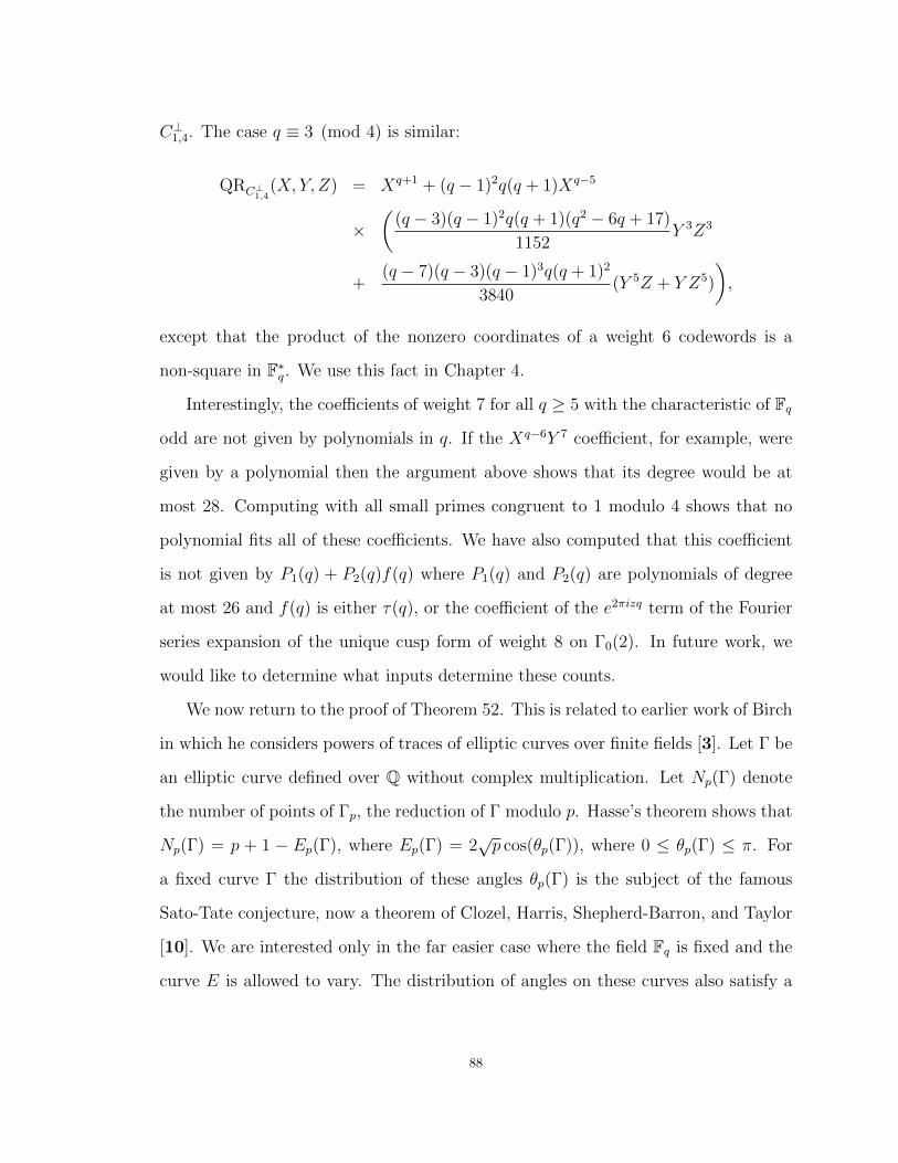
C⊥1,4. The case q ≡ 3 (mod 4) is similar:

QRC⊥1,4(X, Y, Z) = Xq+1 + (q − 1)2q(q + 1)Xq−5

×(

(q − 3)(q − 1)2q(q + 1)(q2 − 6q + 17)

1152Y 3Z3

+(q − 7)(q − 3)(q − 1)3q(q + 1)2

3840(Y 5Z + Y Z5)

),

except that the product of the nonzero coordinates of a weight 6 codewords is a

non-square in F∗q. We use this fact in Chapter 4.

Interestingly, the coefficients of weight 7 for all q ≥ 5 with the characteristic of Fq

odd are not given by polynomials in q. If the Xq−6Y 7 coefficient, for example, were

given by a polynomial then the argument above shows that its degree would be at

most 28. Computing with all small primes congruent to 1 modulo 4 shows that no

polynomial fits all of these coefficients. We have also computed that this coefficient

is not given by P1(q) + P2(q)f(q) where P1(q) and P2(q) are polynomials of degree

at most 26 and f(q) is either τ(q), or the coefficient of the e2πizq term of the Fourier

series expansion of the unique cusp form of weight 8 on Γ0(2). In future work, we

would like to determine what inputs determine these counts.

We now return to the proof of Theorem 52. This is related to earlier work of Birch

in which he considers powers of traces of elliptic curves over finite fields [3]. Let Γ be

an elliptic curve defined over Q without complex multiplication. Let Np(Γ) denote

the number of points of Γp, the reduction of Γ modulo p. Hasse’s theorem shows that

Np(Γ) = p + 1 − Ep(Γ), where Ep(Γ) = 2√p cos(θp(Γ)), where 0 ≤ θp(Γ) ≤ π. For

a fixed curve Γ the distribution of these angles θp(Γ) is the subject of the famous

Sato-Tate conjecture, now a theorem of Clozel, Harris, Shepherd-Barron, and Taylor

[10]. We are interested only in the far easier case where the field Fq is fixed and the

curve E is allowed to vary. The distribution of angles on these curves also satisfy a

88

kind of Sato-Tate distribution that is proven in the following form by Birch [3]. He

focuses only on Fp, but the behavior when q = pf for f > 1 should be similar.

Given an equation of a curve E in Weierstrass form y2 = x3 − ax − b, the trace

of E, p+ 1 minus the number of Fp-rational points, is given by

p+ 1 +

p−1∑x=0

(x3 − ax− b

p

).

This formula holds for elliptic curves as well as for singular curves. Let

SR(p) =

p−1∑a,b=0

(p−1∑x=0

(x3 − ax− b

p

))2R

.

Birch computes that the average over pairs (a, b) of the 2R power of the trace of the

curve in Weierstrass form y2 = x3− ax− b is given by p−2SR(p) +O(pR−1). We gain

information about average values of powers of point counts by studying SR(p).

Theorem 55 (Birch). We have

SR(p) ∼ 2R!

R!(R + 1)!pR+2, as R→∞.

These moments match those of the Sato-Tate distribution. Birch also gives exact

formulas for R ≤ 5, polynomials in p for R ∈ [1, 4] and a polynomial in p minus τ(p)

for R = 5. In order to get these exact formulas he rewrites SR(p) in terms of a sum of

Kronecker class numbers. This sum of Kronecker class numbers can be expressed in

terms of σk(Tp), the trace of the Hecke operator Tp acting on the space of cusp forms

of weight 2 + 2k on SL2(Z). The same strategy applied to dual code coefficients of

weight 2k will prove Theorem 52.

Unfortunately, there is a well-known typo in this paper, so the exact formulas are

off by a small factor [37]. The proof of this result uses a version of the Selberg trace

formula, which we will not discuss here.

89

The connection between powers of traces of elliptic curves and the weight enumer-

ator WG1C (X + (q − 1)Y,X − Y ) should be clear. Each homogeneous quartic f4(x, y)

such that w2 = f4(x, y) defines an elliptic curve E over Fq with #E(Fq) = q + 1− t

contributes a monomial to this weight enumerator, Xq2+q−tq+1Y q3+tq−1. Substituting

X + (q − 1)Y for X and X − Y for Y shows that this term contributes

(X + (q − 1)Y )q2+q−tq+1(X − Y )q

3+tq−1 (mod Y 11)

to the first 10 dual code coefficients. The Y j term of this expansion can be expressed

in terms of the first j powers of t. Taking the sum over all such quartics shows how

the dual code coefficients are related to these powers of traces.

Consider the sum

S ′R(q) :=∑E/∼

t2k,

where E/ ∼ denotes the sum over all isomorphism classes of elliptic curves E over

Fq where #E(Fq) = q + 1 − t, and the isomorphism classes are counted in inverse

proportion to the size of Aut(E).

The exact counts in [3] use the fact that this sum can be expressed as a linear

combination of the trace of the Hecke operator Tp acting on the full space of cusp

forms of weight 2 + 2k for SL2(Z) where the coefficients are polynomials in p. This

is exactly the fact needed to prove Theorem 52 for fields of prime order.

We point out that this result of Birch is written only for fields of prime order.

For q = pk with k > 1 we should technically replace the statement that A10(q) is

a polynomial in q plus a polynomial in q times τ(q) with the statement that A10(q)

is a polynomial in q plus a polynomial in q times S ′R(q). In future work we plan to

analyze this sum in the prime power case to address this issue.

We will use Proposition 53 in Chapter 4 as part of the proof of Theorem 3. The

contribution of the this non-elementary term involving 10th powers of traces of elliptic

90

curves will exactly cancel with the computation of a certain dual code coefficient.

Therefore, this prime power issue is not relevant to the proof of Theorem 3.

8. Quartic Curves with Non-Isolated Singularities

Our main goal is to find the distribution of point counts as we vary through the q15

varieties in P(2, 1, 1, 1) given by w2 = f4(x, y, z), where f4(x, y, z) is a homogeneous

plane quartic. The discussion of the previous sections gives us a way to understand

the contribution to this weight enumerator from cones over genus one curves given by

w2 = f4(x, y), for example, the contribution coming from quartics f4(x, y, z) where

f4(x, y, z) is actually homogeneous in x and y and has no repeated root. This lets us

compute the weight enumerator WG1C′2,4

(X, Y ) and its contribution to dual codewords

of weight up to 10, WG1C (X + (q − 1)Y,X − Y ) modulo Y 11.

We need to understand the contribution to the weight enumerator coming from

quartics f4(x, y, z) with non-isolated singularities. We first observe that a cone over

a variety w2 = f4(x, y) where f4(x, y) is singular has a non-isolated singularity. We

know that f4(x, y) is singular if and only if it has a double root. If f4(x, y) has a

root of multiplicity at least two, the cone contains a line with the same multiplicity.

Therefore, when we consider the contribution to the weight enumerator coming from

varieties of the form w2 = f4(x, y), we want to also assume that f4(x, y) is nonsingular,

that this equation gives a genus 1 curve.

We recall that the contribution to this weight enumerator coming from varieties

given by w2 = f4(x, y, z) where f4(x, y, z) has non-isolated singularities is called

W sC′2,4

(X, Y ). We actually give more information, computing the contribution to the

quadratic residue weight enumerator coming from these terms.

This weight enumerator can be divided into two parts. There are quartics with a

double component that do not vanish to degree 2 on a line, and those that do. Let

QRsnLC′2,4

(X, Y, Z) be the contribution from quartics of this first type, and QRsLC′2,4

(X, Y, Z)

91

be the contribution from quartics of the second type. The terms ‘sL’ and ‘snL’ reflect

whether the variety contains a double Fq-rational line.

Lemma 56. We have

QRsnLC′2,4

(X, Y, Z) =q − 1

2(q5 − q2)Xq+1(Y q2 + Zq2) +

q − 1

2

q4 − q2

X(Y q2+q + Zq2+q).

Proof. The only types of quartics that contribute to this sum are double smooth

conics and the union of two Galois-conjugate double lines defined over Fq2 .

The contribution from the double smooth conics is

q − 1

2(q5 − q2)Xq+1(Y q2 + Zq2),

since there are q5 − q2 smooth conics, such a quartic f(x, y, z)2 takes only square

nonzero values, and the number of squares in F∗q is equal to the number of non-

squares, q−12

.

The contribution from double Galois-conjugate Fq2-rational lines is

q − 1

2

q4 − q2

X(Y q2+q + Zq2+q),

since there are q4−q2

such conjugate lines, and f(x, y, z)2 takes only square nonzero

values, and we have q−12

choices of a scalar multiple.

We also single out the contribution from one other type of quartic. The contri-

bution from the union of two Fq-rational double lines is

q − 1

2

(q2 + q + 1)(q2 + q)

2X2q+1(Y q2−q + Zq2−q).

We isolate this term because every other quartic with a non-isolated singularity

contains a unique line with multiplicity two or greater. All lines are equivalent under

automorphisms of P2(Fq). Therefore, we will determine the weight enumerator com-

ing from a particular choice of a fixed double line and the product with each of the

92

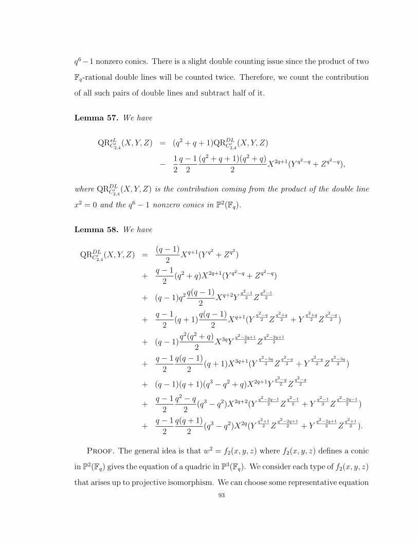
q6−1 nonzero conics. There is a slight double counting issue since the product of two

Fq-rational double lines will be counted twice. Therefore, we count the contribution

of all such pairs of double lines and subtract half of it.

Lemma 57. We have

QRsLC′2,4

(X, Y, Z) = (q2 + q + 1)QRDLC′2,4

(X, Y, Z)

− 1

2

q − 1

2

(q2 + q + 1)(q2 + q)

2X2q+1(Y q2−q + Zq2−q),

where QRDLC′2,4

(X, Y, Z) is the contribution coming from the product of the double line

x2 = 0 and the q6 − 1 nonzero conics in P2(Fq).

Lemma 58. We have

QRDLC′2,4

(X, Y, Z) =(q − 1)

2Xq+1(Y q2 + Zq2)

+q − 1

2(q2 + q)X2q+1(Y q2−q + Zq2−q)

+ (q − 1)q2 q(q − 1)

2Xq+2Y

q2−12 Z

q2−12

+q − 1

2(q + 1)

q(q − 1)

2Xq+1(Y

q2−q2 Z

q2+q2 + Y

q2+q2 Z

q2−q2 )

+ (q − 1)q2(q2 + q)

2X3qY

q2−2q+12 Z

q2−2q+12

+q − 1

2

q(q − 1)

2(q + 1)X3q+1(Y

q2−3q2 Z

q2−q2 + Y

q2−q2 Z

q2−3q2 )

+ (q − 1)(q + 1)(q3 − q2 + q)X2q+1Yq2−q

2 Zq2−q

2

+q − 1

2

q2 − q2

(q3 − q2)X2q+2(Yq2−2q−1

2 Zq2−1

2 + Yq2−1

2 Zq2−2q−1

2 )

+q − 1

2

q(q + 1)

2(q3 − q2)X2q(Y

q2+12 Z

q2−2q+12 + Y

q2−2q+12 Z

q2+12 ).

Proof. The general idea is that w2 = f2(x, y, z) where f2(x, y, z) defines a conic

in P2(Fq) gives the equation of a quadric in P3(Fq). We consider each type of f2(x, y, z)

that arises up to projective isomorphism. We can choose some representative equation

93

for such a quartic and determine the number of points on the corresponding quadric

in P3(Fq). We consider the quartic f4(x, y, z) that is f2(x, y, z) times the square of our

chosen linear form and determine how many of the coordinates of the corresponding

codeword are nonzero squares and how many are non-squares. Suppose that this

linear form defines a line L in P2(Fq). We then consider the restriction of f2(x, y, z)

to L. Combining our knowledge of the quadric in P3(Fq) given by w2 = f2(x, y, z) with

our knowledge of the f2(x, y, z) restricted to L lets us determine the contribution to

the weight enumerator from the quartic f4(x, y, z). Since this restriction of f2(x, y, z)

to L gives a quadratic polynomial on P1(Fq), there are not too many cases to consider.

We explain each term that appears in the statement of this lemma in order. We

first consider double lines. We choose the square of the linear form defining L. This

vanishes at all q + 1 points and takes square values at the other q2 points of P2(Fq).

Multiplying by a non-square gives an equation that vanishes at exactly q + 1 points

and otherwise takes non-square values. Now we consider a polynomial defining the

union of two distinct Fq-rational lines. Such a variety has 2q+ 1−Fq rational points.

The square of such a polynomial takes nonzero values that are all squares or all non-

squares depending on which nonzero scalar we choose. There are q2 + q lines distinct

from L.

For the next term, we consider a polynomial defining the product of two Galois-

conjugate lines with their Fq-rational point of intersection not lying on L. This

gives q+2 total Fq-rational points. There are q4−q2

pairs of Galois-conjugate lines and

q4−q2

q2

q2+q+1= q4−q3

2of them intersect off our given line. This implies that q3−q

2of them

do intersect on L. This polynomial restricts to a quadric with two Galois-conjugate

roots on L. The contribution from the q + 1 points of L is Yq+12 Z

q+12 . The quadric

in P3(Fq) coming from a pair of Galois-conjugate lines is a quadric cone, which has

q2 + q + 1 Fq-rational points. Therefore, since we have q + 2 rational zeros, there

must be q2+q+1−(q+2)2

= q2−12

nonzero square values taken by this polynomial. This

94

means that there are just as many nonzero non-square values. This completes the

explanation for this term.

For the next term, corresponding to the q3−q22

pairs of Galois-conjugate lines with

their point of intersection on L, we note that there are now only q+ 1 Fq-points, and

that this polynomials restricted to L has a double root. The contribution of such a

polynomial restricted to L is either XY q or XZq depending on the restriction of this

conic to L, whether it is a square in F∗q times a square, or a non-square in F∗q times

a square. Each of these possibilities arises equally often. The resulting quadric in

P3(Fq) is a cone with q2 + q + 1 points, so there are either q2−((2q+1)−(q+1))2

= q2−q2

coordinates that are squares, or q2−(1−(q+1))2

= q2+q2

such coordinates.

The next term corresponds to the union of two distinct Fq-rational lines. We

consider two cases based on whether or not the point of intersection of these two

lines lies on L. First suppose that it does not. There are q2 choices for the point

of intersection and (q+1)q2

pairs of distinct Fq-rational lines intersecting at that point.

This polynomial restricted to L has two Fq-rational zeros, so the contribution to

the quadratic residue weight enumerator from the points of L is X2Yq−12 Z

q−12 . The

quadric in P3(Fq) coming from this union of lines is a cone. Therefore there must be

q2+q+1−3q2

= q2−2q+12

nonzero coordinates that are squares and the same number of

non-squares.

Now, if the intersection of our two Fq-rational lines lies on L, this quartic has

3q + 1 rational points. The polynomial defining this union of lines restricts to a

polynomial with a double root on L, which contributes either XY q or XZq to our

weight enumerator depending on which scalar multiple we take. The resulting quadric

in P3(Fq) is a cone. There are either q2+q+1−(3q+1)−(1−(q+1))2

= q2−q2

coordinates that

are nonzero squares, or q2+q+1−(3q+1)−(2q+1−(q+1)2

= q2−3q2

coordinates that are nonzero

squares. Each of these possibilities occurs equally often.

95

The next term breaks down into two pieces. We first consider when the polynomial

gives a union of two Fq-rational lines, exactly one equal to L. There are q(q+ 1) such

pairs of lines. This polynomial is identically 0 when restricted to L and the quadric

in P3(Fq) resulting from it is again a cone. There are q2+q+1−(2q+1)2

= q2−q2

coordinates

that are squares, so there is the same number of non-squares.

Finally, we consider smooth conics intersecting L. We point out that the variety

w2 = f2(x, y, z) where f2(x, y, z) defines a smooth conic in P2(Fq) is a smooth quadric

in P3(Fq). So, it is either a plus quadric, isomorphic to P1(Fq)×P1(Fq) with (q+ 1)2

rational points, or a minus quadric with q2 + 1 points.

First we consider conics that are tangent to the line L at some point. There

are (q5 − q2)(q + 1) pairs of a smooth conic in P2(Fq) along with a Fq-rational line

tangent to it at a point. Dividing by the number of lines and then again by the

number of points on L, there are q2(q − 1) smooth conics tangent to L at a given

point. We note that each point of P2(Fq) not on L lies on a unique line through

the point of tangency and another Fq-rational point on the conic. We see that the

contribution to the quadratic residue weight enumerator of the conic on any such line

is X2Yq−12 Z

q−12 , since it must restrict to a polynomial on this line with two distinct

Fq-points. Summing over the q lines shows that a conic tangent to a point of L

contributes X2q+1Yq(q−1)

2 Zq(q−1)

2 .

We next consider smooth conics that intersect L at two Galois-conjugate points.

There are q2−q2

such pairs of points on L, and q4−q2

total such pairs of points. Each

smooth conic passes through q + 1 Fq-rational points and q2 + 1 Fq2-rational points,

so it must pass through q2−q2

pairs of Galois-conjugate Fq2-points. Therefore we have

(q5− q2)( q2−q2

) pairs of a smooth conic and a pair of conjugate points on it. Dividing

by q4−q2

, we see that there are q2(q−1) smooth conics through a given pair of conjugate

points.

96

The restriction to L of the polynomial defining a smooth conic passing through

two conjugate points on L gives q+12

nonzero squares and the same number of non-

squares. We choose any rational point of this conic and consider all of the lines passing

through it. Every point in P2(Fq) aside from this chosen point is on a unique such

line. We see that q of these lines pass through another Fq-point of the conic, but the

tangent line does not. Each of these q lines contributes X2Yq−12 X

q−12 to the quadratic

residue weight enumerator. The tangent line contributes either XY q or XZq, each

possibility occurring equally often as we vary over the q − 1 scalar multiples of the

conic. We must adjust the quadratic residue weight enumerator to account for the

restriction of the conic to L. Instead of the term Yq+12 Z

q+12 coming from the conic

restricted to L, we have Xq+1 from L. Therefore, this quartic contributes

X2q+2Y q q−12− q+1

2+qZq q−1

2− q+1

2 ,

to the quadratic residue weight enumerator if the polynomial defining the conic re-

stricts to a square in F∗q times a square on the line tangent to the chosen Fq-point,

and the same term but with Y and Z switched otherwise.

Finally, we consider smooth conics passing through two distinct rational points of

L. There are (q2+q+1)(q2+q)2

pairs of distinct Fq-points, (q+1)q2

of which lie on L. Each

smooth conic passes through (q+1)q2

pairs of Fq-points. Therefore, there are

(q5 − q2) (q+1)q2

(q2+q+1)(q2+q)2

= (q3 − q2),

smooth conics through each pair of Fq-points.

We choose one of the two Fq-rational points in the intersection of the conic and

L, and consider all the lines through it. There are q lines on which the contribution

of the conic restricted to L is X2Yq−12 Z

q−12 , including L. The last of these lines is

tangent to the conic and on this line it either restricts to XY q or XZq with each

possibility occurring equally often. Therefore, the contribution of such quartics to

97

the quadratic residue weight enumerator is

q − 1

2

q(q + 1)

2(q3 − q2)X2q(Y q q−1

2− q−1

2+qZq q−1

2− q−1

2 + Y q q−12− q−1

2 Zq q−12− q−1

2+q).

This completes the proof.

Alternatively, we could have given a proof in the following way. We could argue

from the form of the terms contributing to QRDLC′2,4

(X, Y, Z) that all of its coefficients

will be polynomials in q. By computing QRDLC′2,4

(X, Y, Z) for the first several primes,

say the first 10 odd primes or so, and arguing that the degree of each polynomial

will be at most 6, we can find the coefficient of each term of QRDLC′2,4

(X, Y, Z) by

polynomial interpolation. In the next chapter we will need to solve a similar problem

where the case-by-case analysis is too intricate.

We next turn to the contribution of W sC′2,4

(X, Y ) to the low-weight codewords of

C ′⊥2,4 . We could apply the MacWilliams identity for quadratic residue weight enumer-

ators to gain information about how the coordinates of low-weight dual codewords

split up into nonzero squares and non-squares, however this is more information than

we need. We instead consider

QRsnLC′2,4

(X,X2, 1) + QRsLC′2,4

(X,X2, 1),

homogenized to a polynomial of degree q3 + q2 + q in X and Y . This degree is the

number of points in the weighted projective space P(2, 1, 1, 1) omitting the singular

point. This homogenized polynomial is the W sC′2,4

(X, Y ) defined in Chapter 2. Since

the coefficients of this weight enumerator are polynomials in q, applying the linear

transformation form the MacWilliams identity produces contributions to dual code

coefficients that are also polynomial in q.

98

Theorem 59. W sC′2,4

(X + (q − 1)Y,X − Y ) modulo Y 11 is equal to

(q3 − 1)10∑j=0

Aj(q)

j!Xq3+q2+q−jY j +O(Y 11),

where the values of Aj(q) are:

A0(q) = q5 + q4 + 2 q3 + 1, A1(q) = 0, A2(q) =(q8 − 2 q7 − q6 + q5 + q3 + 1

)q

A3(q) = −(q − 2)(4 q8 − 5 q7 − q6 + 2 q5 − q4 + 2 q3 + 2

)q

A4(q) =(q14 − 8 q12 + 11 q11 + 17 q10 − 68 q9 + 100 q8 − 51 q7 − 20 q6 + 39 q5 − 36 q4 + 18 q3 + 6 q2 − 15 q + 18

)q

A5(q) = −2(q − 2)

(5 q14 − 35 q12 + 45 q11 + 38 q10 − 118 q9 + 156 q8 − 89 q7 − 15 q6 + 57 q5 − 60 q4 + 24 q3

+12 q2 − 14 q + 24

)q

A6(q) =

(q20 − 15 q18 + 10 q17 + 146 q16 − 381 q15 − 234 q14 + 2445 q13 − 3638 q12 − 109 q11 + 6239 q10 − 8730 q9

+6916 q8 − 2040 q7 − 2040 q6 + 3325 q5 − 2280 q4 + 130 q3 + 785 q2 − 770 q + 600

)q

A7(q) = −(q − 2)

(21 q20 − 280 q18 + 210 q17 + 1736 q16 − 3451 q15 − 2093 q14 + 15561 q13 − 21293 q12

+1859 q11 + 28299 q10 − 36317 q9 + 27195 q8 − 8294 q7 − 7047 q6 + 12120 q5 − 9000 q4 + 204 q3

+2982 q2 − 2052 q + 2160

)q

A8(q) =

(q26 − 28 q24 + 21 q23 + 532 q22 − 1414 q21 − 3296 q20 + 18024 q19 − 6236 q18 − 90587 q17

+169532 q16 + 60557 q15 − 609723 q14 + 917659 q13 − 414191 q12 − 677404 q11 + 1373296 q10 − 1181278 q9

+575351 q8 + 30205 q7 − 346262 q6 + 344036 q5 − 143948 q4 − 59143 q3 + 85372 q2 − 56196 q + 35280

)q

A9(q) = −4(q − 2)

(9 q26 − 231 q24 + 189 q23 + 2709 q22 − 5481 q21 − 12990 q20 + 54612 q19 − 17036 q18

−209160 q17 + 365393 q16 + 106430 q15 − 1070395 q14 + 1460443 q13 − 616234 q12 − 921947 q11

+1837128 q10 − 1466383 q9 + 655377 q8 + 59587 q7 − 394022 q6 + 371404 q5 − 167992 q4

−73430 q3 + 96164 q2 − 49104 q + 40320

)q

A10(q) =

(q32 − 45 q30 + 36 q29 + 1500 q28 − 4050 q27 − 20700 q26 + 99498 q25 + 56509 q24 − 1001101 q23

+1206436 q22 + 4319196 q21 − 13616003 q20 + 4281177 q19 + 41588189 q18 − 76832522 q17 + 2845541 q16

+181091943 q15 − 298047467 q14 + 189503865 q13 + 78529809 q12 − 295879830 q11 + 313354185 q10

−176095173 q9 + 34145724 q8 + 47631213 q7 − 62669700 q6 + 38639664 q5 − 5261751 q4

−15015852 q3 + 11671452 q2 − 5973264 q + 3265920

)q.

99

We have now computed two of the key terms needed to understand WDPC′2,4

(X, Y ),

the contribution from cones over genus 1 curves given by w2 = f4(x, y), and from

homogeneous quartics w2 = f4(x, y, z) with non-isolated singularities. In the next

chapter we will consider the contribution coming from the 15-dimensional subcode

of cones over plane quartics, and the counts for dual codewords of weight up to 10.

This dual code calculation will be the most intricate part of the proof of Theorem 3.

9. Other MacWilliams Theorems and Codes from Genus 1 Curves

Before moving on to the proof of Theorem 3 we return to variations of the

MacWilliams theorem coming from character sums. We begin with cubic Gauss

sums.

For p ≡ 1 (mod 3), the prime p factors in Z[ω] where ω is a primitive cube root

of unity, as ππ = p for some prime π ∈ Z[ω]. We have F∗p/(F∗p)3

is a cyclic group of

order three. There is a cubic character χπ(β) taking values 1, ω, ω2 which determines

the coset of β in this group. Let ζp = e2πi/p.

Proposition 60. Let p ≡ 1 (mod 3) be a prime and let ψ be an additive character

on Fq. Let α1, α2, α3 be the roots of the polynomial f(x) = x3 − 3px − Ap, where

4p = A2 + 27B2 and A ≡ 1 (mod 3).

Then ∑x∈Fp

ζx3

p

is one of the roots αi. This is 3G1 + 1 where

G1 =∑

x |χπ(x)=1

ψ(x).

100

The other two roots are 3G2 + 1 and 3G3 + 1 where

G2 =∑

x |χπ(x)=ω

ψ(x), and G3 =∑

x |χπ(x)=ω2

ψ(x).

See Section 12 of Chapter 9 of [27] for a proof.

We can now state our cubic residue version of the MacWilliams Theorem. We

will only state this for codes over prime fields.

Theorem 61. Let C be a linear code of length N over Fp with p ≡ 1 (mod 3) and

let

CRC(W,X, Y, Z) :=∑c∈C

N∏i=1

H(ci),

where c = (c1, . . . , cN) and

H(x) =

W if x = 0

X if χπ(x) = 1

Y if χπ(x) = ω

Z if χπ(x) = ω2

.

Then

CRC(W,X, Y, Y ) =1

|C⊥|CRC⊥(W ′, X ′, Y ′, Y ′′),

where

W ′ = W +p− 1

3(X + 2Y ), X ′ = W +G1X + (G2 +G3)Y,

Y ′ = W +G2X + (G3 +G1)Y, Y ′′ = W +G3X + (G1 +G2)Y.

If c = (c1, . . . , cN) ∈ FNq has α coordinates with ci = 0, β coordinates with

χπ(ci) = 1, γ coordinates with χπ(cj) = ω, and δ coordinates with χπ(ci) = ω2,

then for some ε ∈ Fq with χπ(ε) = ω we see that εc = (εc1, . . . , εcN) has (α, δ, β, γ)

of each of these types of coordinates, and that ε2c has (α, γ, δ, β) of each of these

101

coordinates. Since there are p−13

nonzero elements taking each possible value under

χπ and C is linear, we see that the linear transformation in this statement still holds

if we replace (G1, G2, G3) with (G3, G1, G2) or (G2, G3, G1). We note that it is not

generally equivalent to the linear transformation where (G1, G2, G3) is replaced by

(G2, G1, G3).

Proof. We closely follow the strategy from the proof of the MacWilliams identity

for the quadratic residue weight enumerator given at the beginning of this chapter.

Let φ(c) =∏N

i=1H(ci). So∑

c∈C φ(c) = CRC(W,X, Y, Z). We see that the Fourier

transform of φ is defined by

φ(g) =∑g∈FNp

ψ(〈g, g〉)φ(g).

Discrete Poisson summation gives

∑c∈C

φ(c) =1

|C⊥|∑d∈C⊥

φ(d).

We consider the coordinates of φ(d) one at a time. We have

φ(d) =∑g∈FNp

N∏i=1

ψ(digi)H(gi) =N∏i=1

∑gP∈Fp

ψ(digi)H(gi)

=N∏i=1

W +X∑

x | χπ(x)=1

ψ(xdi) + Y∑x| x 6=0

χπ(x)6=1

ψ(xdi)

.

We consider the internal sum. If di = 0, this is W + p−13

(X + 2Y ). If χπ(dP ) = 1,

this is

W +X∑

x | χπ(x)=1

ψ(x) + Y∑

x | x 6=0

χπ(x)6=1

ψ(x) = W +G1X + (G2 +G3)Y.

102

If χπ(di) = ω, this is

W +X∑

x | χπ(x)=ω

ψ(x) + Y∑

x | x6=0

χπ(x) 6=ω

ψ(x) = W +G2X + (G3 +G1)Y.

Finally, if χπ(di) = ω2, this is

W +X∑

x | χπ(x)=ω

ψ(x) + Y∑

x | x6=0

χπ(x) 6=ω

ψ(x) = W +G3X + (G1 +G2)Y.

Taking the product over all coordinates i and then the sum over all d ∈ C⊥ completes

the proof.

We note that it is not strictly necessary to determine which of the three roots αi

of x3− 3px−Ap satisfies G1 = αi−13

. This is not easy to determine and is the subject

of Kummer’s conjecture for cubic Gauss sums, now a theorem of Heath-Brown [25].

We can simply choose some αi, the largest one for example, and let K1 = αi−13

. Then

we substitute K1 for G1 and (K2, K3) for (G2, G3) where K2 and K3 and given in

terms of the other two roots of the polynomial. One of these choices will lead to an

identity that holds, and the others generally will not.

Just as we studied the quadratic residue weight enumerator for the code of ho-

mogeneous degree 2k forms on Pn(Fq), we can study this cubic weight enumerator

for homogeneous degree 3k forms on Pn(Fq). In the simplest case, k = 1, n = 1,

we get homogeneous cubics on P1(Fq). Like the quadratic residue weight enumerator

applied to quartics on P1(Fq) led to the study of elliptic curves over finite fields, this

setting also gives genus 1 curves, although a more restricted family.

Proposition 62. Let f3(x, y) be a smooth homogeneous cubic on P1(Fp). Then

w3 = f3(x, y) is a genus 1 curve, an elliptic curve with j-invariant 0. Given an ellip-

tic curve E defined over Fp with j-invariant 0 there is a homogeneous cubic f3(x, y)

such that w3 = f3(x, y) is isomorphic to E.

103

Proof. This is a standard fact about elliptic curves given as homogeneous cubics.

For a general discussion of how to take such a cubic and put it into Weierstrass form

see Section 1.4 of [11]. For a general definition of the j-invariant attached to a

nonsingular homogeneous cubic, see the appendix of [18].

In future work we plan to compute CRC(W,X, Y, Z) for this 4-dimensional code

and study the low-weight coefficients of its dual. We can then study the code of

diagonal cubic surfaces w3 = f3(x, y, z) in P3(Fq). The weight enumerator of this

code will contain a contribution from cones over these genus 1 curves of j-invariant

0. It would be interested to compare point counts for these diagonal cubics to point

count for general cubic surfaces.

There is another natural setting for this type of variation of the MacWilliams

identity. Using results on biquadratic Gauss sums we can prove a variation of this

identity that keeps track of whether a coordinate is a 4th power or not modulo p.

This weight enumerator can be applied to the code of quadrics on P1(Fq) leading

to equations of the form w4 = f2(x, y), where f2(x, y) is a quadric on P1(Fq) with

distinct roots. Such an equation defines a genus 1 curve with j-invariant 1728. We

can think of this as a homogeneous quartic in the weighted projective space P(1, 2, 2)

where w has weight 1 and x and y each have weight 2. We plan to pursue this in

future work.

104

CHAPTER 4

The Distribution of Point Counts for del Pezzo Surfaces of

Degree 2

In this chapter we give the proof of Theorem 3. This will involve a computation

of low-weight dual code coefficients for a particular 16-dimensional code, and for a

related 15-dimensional code. We also use the geometry of P2(Fq) and facts about the

Picard group of a del Pezzo surface of degree 2 to determine the number of equations

w2 = f4(x, y, z) with q2 + 8q + 1 Fq-points and with q2 + 7q + 1 Fq-points. We also

describe interesting geometric consequences of Theorem 3 for small values of q.

1. A Sketch of the Proof

We recall the setup from Chapter 2. Let C ′2,4 be the 16-dimensional code coming

from varieties of the form

αw2 = f4(x, y, z),

which we can think of as homogeneous quartics in the weighted projective space

P(2, 1, 1, 1). We also need to consider Cc2,4, the 15-dimensional subcode from varieties

with α = 0.

We write

WC′2,4(X, Y ) = WCc2,4

(X, Y ) + (q − 1)WDC′2,4

(X, Y ),

where WDC′2,4

(X, Y ) is the contribution to the weight enumerator from codewords with

α = 1. We let

WDC′2,4

(X, Y ) = W sC′2,4

(X, Y ) +WG1C′2,4

(X, Y ) +WDPC′2,4

(X, Y ),

105

where W sC′2,4

(X, Y ) is the contribution to this weight enumerator from equations of

the form w2 = f4(x, y, z) where f4(x, y, z) defines a plane quartic with non-isolated

singularities, WG1C′2,4

(X, Y ) is the contribution to this weight enumerator from equa-

tions of the form w2 = f4(x, y, z) where f4(x, y, z) gives the union of four coincident

lines, a quartic curve with a non-simple elliptic singularity, and WDPC′2,4

(X, Y ) is the

contribution to the weight enumerator from everything else. We have seen that

WDPC′2,4

(X, Y ) = a−7Xq2+q+1−(−7q)Y q3−7q−1 + · · ·+ a7X

q2+q+1−(7q)Y q3+7q−1,

where aj = a−j for j ∈ [1, 7].

In this chapter we find these 8 unknowns a0, a1, . . . , a7. A first major step will be

determining the WDPC′2,4

(X + (q − 1)Y,X − Y ) modulo Y 11. It is clear that

WDC′2,4

(X + (q − 1)Y,X − Y ) = W sC′2,4

(X + (q − 1)Y,X − Y )

+ WG1C′2,4

(X + (q − 1)Y,X − Y ) +WDPC′2,4

(X + (q − 1)Y,X − Y ).

The MacWilliams theorem implies that

q16WC′⊥2,4

(X, Y ) = WCc2,4(X + (q − 1)Y,X − Y ) + (q − 1)WD

C′2,4(X + (q − 1)Y,X − Y ),

and

WCc2,4(X + (q − 1)Y,X − Y ) = q15WCc⊥2,4

(X, Y ).

In the previous chapter we computed

W sC′2,4

(X + (q − 1)Y,X − Y ) +WG1C′2,4

(X + (q − 1)Y,X − Y ) (mod Y 11).

Therefore, in order to compute WDPC′2,4

(X + (q − 1)Y,X − Y ) modulo Y 11 we instead

find WC′⊥2,4

(X, Y ) modulo Y 11 and WCc⊥2,4(X, Y ) modulo Y 11.

We first state our main results and postpone the proofs until later.

106

Theorem 63. WCc⊥2,4(X, Y ) modulo Y 11 is equal to

Xq3+q2+q + (q − 1)2q(q2 + q + 1)10∑j=2

Aj(q)

j!Xq3+q2+q−jY j +O(Y 11),

where the values of Aj(q) are:

A2(q) = 1, A3(q) = (q − 2)2

A4(q) = (3 q5 − 2 q4 − 11 q3 + 27 q2 − 33 q + 18)

A5(q) = (q − 2)2(10 q5 − 9 q4 − 19 q3 + 38 q2 − 38 q + 24

)A6(q) = (16 q10 − 13 q9 − 237 q8 + 863 q7 − 1108 q6 − 274 q5 + 2790 q4 − 4180 q3 + 3525 q2 − 1970 q + 600)

A7(q) = (q − 2)

(q12 + 109 q11 − 452 q10 − 124 q9 + 3725 q8 − 8267 q7 + 6270 q6 + 5699 q5 − 18472 q4

+21651 q3 − 15312 q2 + 7452 q − 2160

)A8(q) =

(q16 + 135 q15 − 138 q14 − 4625 q13 + 22564 q12 − 32694 q11 − 52554 q10 + 287862 q9 − 490272 q8

+318928 q7 + 277242 q6 − 881251 q5 + 1056237 q4 − 807919 q3 + 430360 q2 − 162036 q + 35280

)A9(q) = (q − 2)

(q18 + 40 q17 + 1382 q16 − 8928 q15 + 491 q14 + 129139 q13 − 415145 q12 + 358839 q11

+953277 q10 − 3280584 q9 + 4232208 q8 − 1611694 q7 − 3300122 q6 + 6798764 q5 − 6798260 q4

+4587408 q3 − 2201072 q2 + 760896 q − 161280

)A10(q) =

(q22 + 48 q21 + 1734 q20 − 5599 q19 − 86758 q18 + 641336 q17 − 1337083 q16 − 2292639 q15

+18254124 q14 − 39440054 q13 + 21366100 q12 + 84882388 q11 − 239151303 q10 + 290151336 q9

−123793500 q8 − 178740396 q7 + 406197288 q6 − 433630392 q5 + 312483609 q4 − 166440924 q3

+66046428 q2 − 19036944 q + 3265920

).

107

Theorem 64. WC′⊥2,4

(X, Y ) modulo Y 11 is equal to

Xq3+q2+q + (q − 1)2(q2 + q + 1)10∑j=2

Aj(q)

j!Xq3+q2+q−jY j +O(Y 11),

where the values of Aj(q) are:

A2(q) = 1, A3(q) = (q − 3)(q − 2)

A4(q) = (3 q5 − 2 q4 − 11 q3 + 30 q2 − 48 q + 36)

A5(q) = (q − 2)(10 q6 − 29 q5 − q4 + 76 q3 − 120 q2 + 142 q − 120

)A6(q) = (16 q10 − 13 q9 − 236 q8 + 854 q7 − 1073 q6 − 329 q5 + 2804 q4 − 4256 q3 + 4195 q2 − 3510 q + 1800)

A7(q) = (q − 2)

(q12 + 109 q11 − 452 q10 − 124 q9 + 3704 q8 − 8078 q7 + 5640 q6 + 6539 q5 − 18466 q4

+20892 q3 − 16467 q2 + 12582 q − 7560

)A8(q) =

(q16 + 135 q15 − 138 q14 − 4625 q13 + 22565 q12 − 32721 q11 − 52050 q10 + 283431 q9 − 470154 q8

+268885 q7 + 340997 q6 − 899977 q5 + 1005543 q4 − 770224 q3 + 510076 q2 − 330624 q + 141120

)A9(q) = (q − 2)

(q18 + 40 q17 + 1382 q16 − 8928 q15 + 491 q14 + 129139 q13 − 415265 q12 + 360567 q11

+939809 q10 − 3210332 q9 + 3988076 q8 − 1086638 q7 − 3894778 q6 + 6900916 q5 − 6222468 q4

+3976924 q3 − 2277288 q2 + 1448352 q − 725760

)A10(q) =

(q22 + 48 q21 + 1734 q20 − 5599 q19 − 86758 q18 + 641337 q17 − 1336992 q16 − 2294532 q15

+18273165 q14 − 39568799 q13 + 22020658 q12 + 82256547 q11 − 230767899 q10 + 269456593 q9

−86914540 q8 − 219872635 q7 + 421463214 q6 − 404765268 q5 + 263019501 q4 − 138762972 q3

+74629836 q2 − 42930000 q + 16329600

)− (q − 1)(q + 1)q5τ(q).

Combining these results with the computations of W sC′2,4

(X + (q − 1)Y,X − Y ))

and WG1C′2,4

(X + (q − 1)Y,X − Y ), both modulo Y 11, gives the following statement.

Corollary 65. WDPC′2,4

(X + (q − 1)Y,X − Y ) modulo Y 11 is given by

A0(q) + (q3 − 1)(q2 − q)10∑j=2

Aj(q)

j!Xq3+q2+q−jY j +O(Y 11),

108

where the values of Aj(q) are:

A0(q) = (q15 − q8 − 2 q7 − 2 q6 + 2 q5 + 2 q4 + q3 − q2 + 1),

A2(q) = (−2 q8 + 3 q7 + 3 q6 − 2 q5 − 2 q4 − q3 + q2 − 1)

A3(q) = −(q − 2)(q15 − 7 q8 + 7 q7 + 7 q6 − 4 q5 − 4 q4 − 2 q3 + 2 q2 − 2

)A4(q) =

(3 q17 − 15 q16 + 18 q15 − q14 − 2 q13 + 14 q12 − 9 q11 − 39 q10 + 104 q9 − 121 q8 + 3 q7 + 87 q6 − 12 q5

−12 q4 − 33 q3 + 12 q2 + 15 q − 18

)A5(q) = −2(q − 2)

(3 q17 − 21 q16 + 36 q15 − 5 q14 − 10 q13 + 60 q12 − 30 q11 − 108 q10 + 160 q9 − 150 q8 + 31 q7

+102 q6 − 32 q5 − 12 q4 − 38 q3 + 12 q2 + 14 q − 24

)A6(q) =

(q23 − 9 q22 + 35 q21 − 56 q20 + 14 q19 − 66 q18 + 690 q17 − 1717 q16 + 1356 q15 + 1246 q14 − 3925 q13

+2918 q12 + 4414 q11 − 9606 q10 + 7670 q9 − 4010 q8 − 770 q7 + 3260 q6 − 1315 q5 + 665 q4 − 900 q3

−185 q2 + 770 q − 600

)A7(q) = − (q − 2)

(21 q23 − 189 q22 + 630 q21 − 861 q20 − 6 q19 + 934 q18 + 1505 q17 − 7307 q16 + 6296 q15

+9709 q14 − 22953 q13 + 14356 q12 + 21954 q11 − 41875 q10 + 25181 q9 − 13479 q8 + 1938 q7 + 11352 q6

−7002 q5 + 2262 q4 − 2256 q3 − 822 q2 + 2052 q − 2160

)A8(q) =

(q27 − 28 q26 + 504 q25 − 4403 q24 + 20083 q23 − 50435 q22 + 64791 q21 − 16992 q20 − 54354 q19

+5384 q18 + 184751 q17 − 187551 q16 − 318878 q15 + 897732 q14 − 667990 q13 − 408570 q12 + 1350580 q11

−1213422 q10 + 575302 q9 − 243789 q8 − 106414 q7 + 334726 q6 − 192759 q5 + 52920 q4 + 2947 q3

−50092 q2 + 56196 q − 35280

)A9(q) = −4(q − 2)

(30 q27 − 441 q26 + 3367 q25 − 17332 q24 + 60718 q23 − 132818 q22 + 151373 q21 − 18437 q20

−150512 q19 + 66250 q18 + 243915 q17 − 177979 q16 − 663788 q15 + 1431957 q14 − 849396 q13 − 671948 q12

+1755992 q11 − 1455636 q10 + 574117 q9 − 287264 q8 − 41684 q7 + 405176 q6 − 255402 q5 + 42396 q4

+24326 q3 − 55844 q2 + 49104 q − 40320

)A10(q) =

(91 q31 − 1848 q30 + 19005 q29 − 130287 q28 + 659238 q27 − 2608159 q26 + 8276211 q25

−20599432 q24 + 37219965 q23 − 41516259 q22 + 14127321 q21 + 27031378 q20 − 28077430 q19

−14089496 q18 + 5884299 q17 + 121271322 q16 − 255860130 q15 + 197868984 q14 + 51768804 q13

−266034654 q12 + 289927485 q11 − 169439655 q10 + 61973298 q9 − 14150610 q8 − 37966077 q7

+57749445 q6 − 24347772 q5 − 2662317 q4 + 9042588 q3 − 8405532 q2 + 5973264 q − 3265920

)q.

109

We are very fortunate that even though both WG1C′2,4

(X + (q − 1)Y,X − Y ) and

WC′⊥2,4

(X, Y ) have a Y 10 term that involves τ(q), these non-elementary contributions

cancel out, leaving counts for WDPC′2,4

(X + (q − 1)Y,X − Y ) that are polynomial in q.

We have 11 constraints given by the Y j coefficient of WDPC′2,4

(X + (q− 1)Y,X − Y )

for each j ∈ [0, 10] and 8 unknowns aj for j ∈ [0, 7]. It is easy to see that not every

dual coefficient gives a new constraint. For example, the fact that the Y 1 coefficient

is 0 is implied by the condition that aj = a−j. The fact that these constraints are not

independent is one of the key differences between this computation and the analogous

one for del Pezzo surfaces of degree 3.

For each j ∈ [1, 7] we consider the Taylor series expansion of

((X + (q − 1)Y )q2+q+1−qj(X − Y )q

3−qj−1 + (X + (q − 1)Y )q2+q+1+qj(X − Y )q

3+qj−1

in the variable Y . The Y 1 term is equal to 0, but we use Y 0 and then Y k for

k ∈ [2, 10] to create a column vector for each j with 10 entries. For j = 0 we consider

the expansion of (X + (q− 1)Y )q2+q+1(X − Y )q

3−1, again omitting the Y 1 term. The

rows of the resulting matrix correspond to increasing powers of Y .

We multiply this 10× 8 matrix by a column vector with entries a0, a1, . . . , a7 and

try to solve the matrix equation where this is equal to the column vector with entries

given by Corollary 65. One would hope that this system of linear equations in the aj

is uniquely determined; that is what happens in the analogous computation for cubic

surfaces. Unfortunately, a computation shows that this matrix only has rank 6.

Therefore, if we can find the values of a7 and a6 we can adjust this matrix equation

and hope for a unique solution. This gives a modified version of the column vector

with entries given by Corollary 65 consisting only of the contribution to these values

from a0, . . . , a5. Once we have solved for a6 and a7, this will give a system where

we multiply a 10 × 6 matrix by a column vector with entries, a0, a1, . . . , a5 and get

this modified version of the vector with entries from Corollary 65 as the result. This

110

matrix has rank 6 and we get a unique solution. This solution is the content of

Theorem 3.

For the particular case q = 5 we get

a7 = a6 = 0, a5 = 7750, a4 = 2728000, a3 = 119977750,

a2 = 1646534000, a1 = 7426406500, a0 = 12125699601.

This matches our direct computation of the weight distribution of the 516 elements

of the code C ′2,4 over F5. This took over a day of computing time and is the last case

where this computation is feasible using our current implementation. Later in this

chapter we return to this example and explain the value a5 = 7750. We also study

these counts for other small values of q.

2. Del Pezzo Surfaces of Trace 7 and 6

The goal of this section is to give a proof of Theorem 27. First we consider the

easier case of surfaces of trace 7. We show that these surfaces come from blowing

up seven points in P2(Fq) in general position. We then count how many times each

surface arises from blowing up such a 7-tuple. Next, we show that surfaces of trace 6

come from blowing up seven points in P2(Fq) in near general position. Given such a

weak del Pezzo surface S we study Pic(S) to determine the number of ways S arises

from blowing up seven such points. In this case, the lattice generated by (−2)-curves

of S is one-dimensional, so we must study the action of the Weyl group of E7 on

Pic(S) in more detail.

Let S be a weak del Pezzo surface of degree 2. By Proposition 24, the number of

Fq-rational solutions of the anti-canonical model of S is q2 + q + 1 + tq, where

t = Tr(ϕ|E7)− Tr(ϕ|R) = Tr(ϕ|R⊥),

111

ϕ is the Frobenius endomorphism and R is the sublattice of Pic(S) generated by

(−2)-curves. Since Tr(ϕ|E7) takes values between −7 and 7, but not ±6, and t is

bounded in absolute value by dim(R⊥), we see that t = 7 if and only if R is trivial

and Tr(ϕ|E7) = 7. Moreover, we see that t = 6 implies that R is one-dimensional.

Since R is a root lattice, it is isomorphic to A1.

In order to determine a7 and a6 we give some information about the 2 : 1 map

φ : S → P2. Suppose that S is the blow-up of points p1, . . . , p7 in P2(Fq). We would

like to determine how many equations of the form w2 = f4(x, y, z) arise from S.

We recall some facts from Proposition 11. There is a 3-dimensional space of cubics

vanishing at p1, . . . , p7. We choose a basis for this space, and call these cubics x, y, z.

We can choose these coordinates in |PGL3(Fq)| ways.

There is a 7-dimensional space of sextic polynomials vanishing to order 2 at each

pi. Any such sextic w not in the space spanned by quadratic polynomials in x, y and

z, 〈x2, xy, xz, y2, yz, z2〉, satisfies an equation of the form

w2 − w · f2(x, y, z)− f4(x, y, z) = 0,

where f2(x, y, z) is quadratic, and f4(x, y, z) is a homogeneous quartic. We want a

sextic for which the polynomial f2(x, y, z) is zero. This gives six linear conditions,

leading to a 1-dimensional space. We must not choose w = 0, so we have q−1 choices

for w.

We recall that the number of 7-tuples of points in P2(Fq) in general position is

given by S(q)|PGL3(Fq)| and the number of 7-tuples in near general position is given

by R(q)|PGL3(Fq)|.

We now give the proof of the trace 7 case.

Proof. A weak del Pezzo surface with q2 + q + 1 + 7q points is the blow-up of

seven Fq-points of P2(Fq) in general position. Consider the surfaces we get by blowing

112

up all such 7-tuples. We saw in the previous paragraph that one such 7-tuple gives

rise to |GL3(Fq)| quartics w2 = f4(x, y, z).

A homogeneous quartic w2 = f4(x, y, z) with q2 + q+ 1 + 7q Fq-points is the anti-

canonical model of a smooth del Pezzo surface S. We want to know the number of

blowing-down structures of this surface. The 28 bitangent lines of the branch quartic

f4(x, y, z) are the images of the (−1)-curves of S under φ. The quartic restricted to

one of these lines is a perfect square. Choosing a value of w is equivalent to choosing

which square root we take on such a quartic. Taking seven pairwise-skew (−1)-curves

on S gives a geometric basis H, e1, . . . , e7 for Pic(S). Because the divisor classes

must satisfy ei · ej = 0 for i 6= j, we cannot choose these square roots arbitrarily for

each bitangent.

Blowing up each tuple in general position and choosing coordinates for the anti-

canonical model of the resulting surface gives

|PGL3(Fq)|S(q)|GL3(Fq)|

homogeneous quartics w2 = f4(x, y, z). However, we have over-counted. A surface S

arises as the blow-up of more than one 7-tuple.

Starting from a tuple p1, . . . , p7, blowing up gives a surface S and a canonical

root basis for Pic(S), or equivalently, a blowing-down structure for S. Starting with

an equation of the form w2 = f4(x, y, z) with f4(x, y, z) smooth, we can find the

bitangents of the quartic and take the preimages under this φ. Any set of seven

pairwise disjoint (−1)-curves gives a canonical root basis for Pic(S), or equivalently,

a blowing-down structure of S. We have seen that the Weyl group of E7 acts simply

transitively on these canonical root bases, so the number of blowing-down structures

of S is equal to |W (E7)|.

The smooth surface S arises as the blow-up of seven points in general position in

exactly |W (E7)| ways. A blowing-down structure gives points in P2(Fq), p1, . . . , p7,

113

but it does not give a canonical choice of coordinates for this space. There are

|PGL3(Fq)| choices for these coordinates. Therefore, we get

a7 =|PGL3(Fq)|S(q)|GL3(Fq)||PGL3(Fq)||W (E7)|

,

completing the proof of the statement for a7.

We now turn to the more complicated case, surfaces of trace 6.

Proof. Given a weak del Pezzo surface S of degree 2, the number of points on

the anti-canonical model of S is q2 + q+ 1 + tq, for t = Tr(ϕ|E7)−Tr(ϕ|R), where R

is the sublattice of E7 generated by the (−2)-curves of S. We have seen above that if

t = 6, then R is one-dimensional and Tr(ϕ|E7) = 7. So there is a unique (−2)-curve

of S. Since R is a root sublattice of E7, it is isomorphic to A1. All sublattices A1 are

equivalent under automorphisms of E7.

Given any geometric basis of Pic(S), H, e1, . . . , e7, consider the divisor class

D = 2H − (e1 + · · · e6). This satisfies

D ·D = 4H ·H +6∑i=1

ei · ei = 4− 6 = −2.

Recall that the anti-canonical class is given by

K = 3H − (e1 + · · ·+ e7),

and that the orthogonal complement of K in Pic(S) is isomorphic to E7. It is easy

to verify that D · K = 0. Since D has norm −2 this divisor class generates an

A1 sublattice in E7. By taking an automorphism of E7 we may suppose that the

sublattice R generated by the (−2)-curve of S is generated by D. Blowing up a

7-tuple of points p1, . . . , p7 in near general position gives a weak del Pezzo surface S

with a geometric basis such that D is the class of the (−2)-curve on S exactly when

p1, . . . , p6 lie on a conic not containing p7. This is the case for exactly 1/7 of the

114

7-tuples in near general position. The orthogonal complement of A1 in E7 is D6. The

direct sum A1⊕D6 is contained in E7 with index 2. The presence of this (−2)-curve

gives this decomposition.

We now determine how many blowing-down structures for S give a 7-tuple in near

general position. Suppose we have a geometric basis H, e1, . . . , e7 for Pic(S) and a

sublattice A1 generated by the divisor D = 2H − (e1 + · · · e6). Let ri = ei− K2

. Then

ri ·K = ei ·K −K ·K

2= 0.

We also have

ri · rj =

(ei −

K

2

)·(ej −

K

2

)= −δij − 1 +

K ·K4

= −δij −1

2.

These ri are not in E7 because they are not in the integer span of our basis, but they

are in the dual lattice, E∗7 .

We note that E7 ⊂ E∗7 with index 2. We consider the orthogonal complement of

A1 in E∗7 . This contains the D6 in E7 with index 2. This orthogonal complement in

E∗7 is contained in this D∗6 ⊂ E∗7 with index 2. We can verify these index statements

by computing discriminants of the relevant lattices. This gives the following picture:

E7 ⊂ E∗7

∪ ∪

A⊥1 = D6 ⊂ A⊥1 in E∗7 ⊂ D∗6

.

The class r7 is distinguished from r1, . . . , r6 by its intersection with D. We have

r7 ·D = 0 and ri ·D = ei ·D − K·D2

= 1 otherwise. We see that (ri + D2

) ·D = 0 for

i ∈ [1, 6]. Therefore, we have 7 vectorsr7, r1 +

D

2, . . . , r6 +

D

2

115

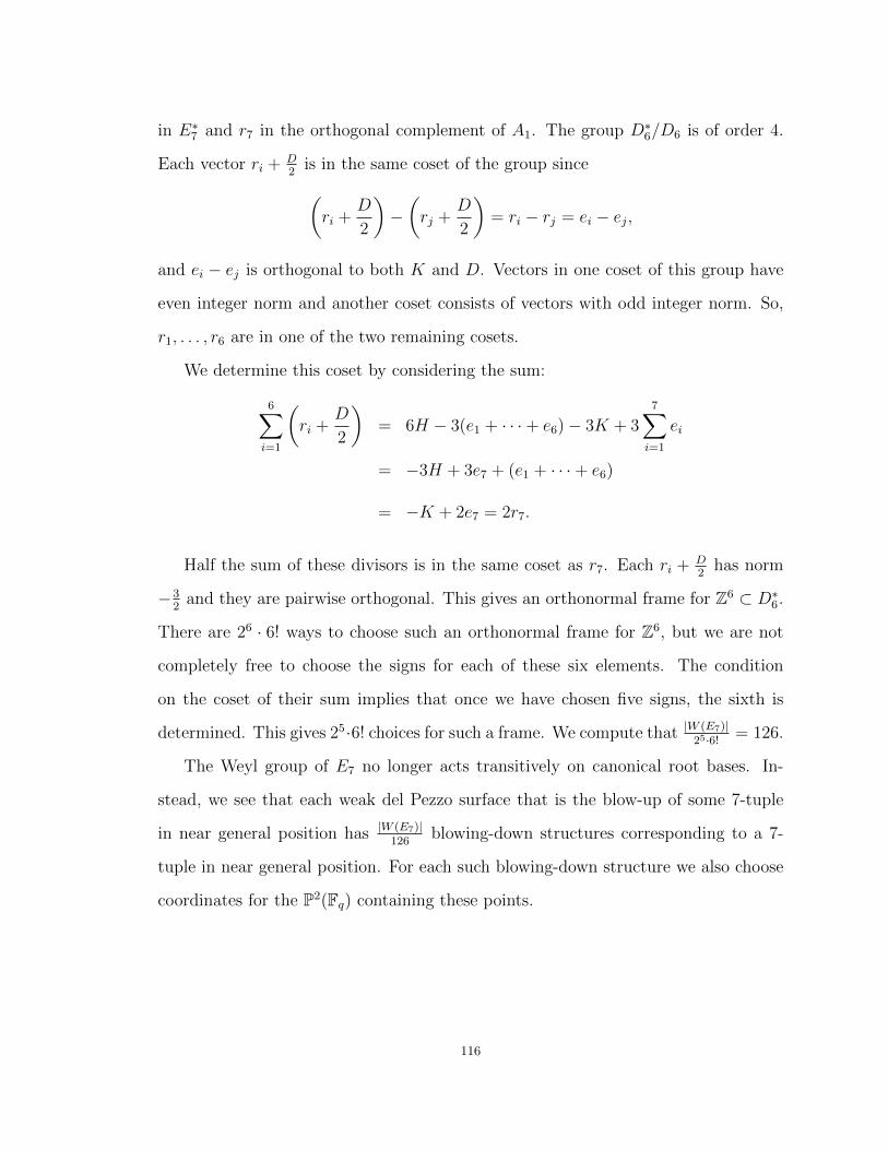
in E∗7 and r7 in the orthogonal complement of A1. The group D∗6/D6 is of order 4.

Each vector ri + D2

is in the same coset of the group since(ri +

D

2

)−(rj +

D

2

)= ri − rj = ei − ej,

and ei − ej is orthogonal to both K and D. Vectors in one coset of this group have

even integer norm and another coset consists of vectors with odd integer norm. So,

r1, . . . , r6 are in one of the two remaining cosets.

We determine this coset by considering the sum:

6∑i=1

(ri +

D

2

)= 6H − 3(e1 + · · ·+ e6)− 3K + 3

7∑i=1

ei

= −3H + 3e7 + (e1 + · · ·+ e6)

= −K + 2e7 = 2r7.

Half the sum of these divisors is in the same coset as r7. Each ri + D2

has norm

−32

and they are pairwise orthogonal. This gives an orthonormal frame for Z6 ⊂ D∗6.

There are 26 · 6! ways to choose such an orthonormal frame for Z6, but we are not

completely free to choose the signs for each of these six elements. The condition

on the coset of their sum implies that once we have chosen five signs, the sixth is

determined. This gives 25·6! choices for such a frame. We compute that |W (E7)|25·6!

= 126.

The Weyl group of E7 no longer acts transitively on canonical root bases. In-

stead, we see that each weak del Pezzo surface that is the blow-up of some 7-tuple

in near general position has |W (E7)|126

blowing-down structures corresponding to a 7-

tuple in near general position. For each such blowing-down structure we also choose

coordinates for the P2(Fq) containing these points.

116

Blowing up all 7-tuples in near general position such that p1, . . . , p6 lie on a conic

not containing p7 and then choosing coordinates for the 2 : 1 map to P2 gives

|PGL3(Fq)|R(q)|GL3(Fq)|

7

homogeneous quartics w2 = f4(x, y, z) with q2 +7q+1 solutions in P(2, 1, 1, 1). Given

such a quartic there are 25 ·6!|PGL3(Fq)| blowing-down structures that give a 7-tuple

in near general position. Dividing gives

a6 =18|GL3(Fq)|R(q)

|W (E7)|,

completing the proof.

Finally, we must compute S(q) and R(q). We begin with a discussion of k-arcs in

P2(Fq). A subset of points S ⊂ P2(Fq) is called an arc if no three points of S lie on a

line. A k-arc is a collection of k distinct points that form an arc. It is elementary to

give a count for k-arcs for k up to 6. For example, suppose p1, . . . , p5 form a 5-arc.

There are(

52

)= 10 distinct lines between these points. Each line contains two of

these five points and q − 1 other points. It is not difficult to show that there are

10q− 20 distinct points on these lines. Therefore, given a 5-arc there are q2− 9q+ 21

choices of another point of P2(Fq) so that the resulting collection forms a 6-arc. This

count is independent of the choice of 5-arc. The following counts for k-arcs are given

in Theorem 4.1 of [23].

Proposition 66. Let A(k, q) denote the number of k-arcs in P2(Fq). Then

A(1, q) = q2 + q + 1, A(2, q) =A(1, q)(q2 + q)

2,

A(3, q) = A(2,q)q2

3, A(4, q) =

A(3, q)(q − 1)2

4,

A(5, q) = A(4,q)(q−2)(q−3)5

, A(6, q) =A(5, q)(q2 − 9q + 21)

6.

117

Counting 7-arcs leads to new difficulties. Starting with a 6-arc p1, . . . , p6, the

number of choices of p7 leading to a 7-arc depends on the choice of p1, . . . , p6. This

is also the first case where the count is not a polynomial in q. The function A(7, q)

is a polynomial in q plus a term involving the number of copies of P2(F2) in P2(Fq),

which is zero if the characteristic of Fq is not equal to 2. Therefore, A(7, q) is a

polynomial in q as long as we exclude characteristic 2. For details, see [23]. The

following result is Theorem 4.2 of that paper.

Proposition 67. Let (73) denote the number of copies of P2(F2) in P2(Fq). Then

A(7, q) =1

7!(q2 + q + 1)(q + 1)q3(q − 1)2(q − 3)(q − 5)

× (q4 − 20q3 + 148q2 − 468q + 498)− (73).

In order to compute S(q) we need to understand how many of these 7-arcs satisfy

the additional condition that no six points lie on a conic. It is easy to count the

number of collections of seven points that lie on a smooth conic in P2(Fq). This is

the number of smooth conics, q5 − q2, times(q+1

7

). We call this quantity C7(q). It

follows that A(7, q) = S(q) +R(q) + C7(q), giving

S(q)+R(q) =1

7!(q2 +q+1)(q2 +q)q2(q−1)2(q−3)(q−5)(q−7)(q3−13q2 +56q−70).

The factor of (q2 + q + 1)(q2 + q)q2(q − 1)2 = |PGL3(Fq)| comes from fixing the first

four points of the configuration. We find R(q) and subtract to get S(q).

Lemma 68. We have

S(q) = (q − 7)(q − 5)(q − 3)(q3 − 20q2 + 119q − 175),

and that

R(q) = 7(q − 7)(q − 5)(q − 3)(q2 − 9q + 15).

118

Proof. There are q5−q2 smooth conics in P2(Fq), all equivalent under PGL3(Fq).

We fix one such conic C and count collections of points p1, . . . , p6 on C and p7 not

on C such that p1, . . . , p7 form a 7-arc. We first consider the number of choices of

p7. For any p7 6∈ C, there are two tangent lines to C passing through it. They are

either both rational, or are Galois-conjugate. There are q2 points not on C, q(q+1)2

of

which lie on two Fq-rational tangent lines to C. The other q(q−1)2

points lie on two

Galois-conjugate tangent lines.

First suppose that p7 does not lie on any Fq-rational tangent line. Then the line

between any Fq-point p of C and p7 passes through one other Fq-point of C, which

we call p′. If both p and p′ are in p1, . . . , p6 then p1, . . . , p7 is not a 7-arc. So,

the q + 1 rational points of C split into q+12

pairs. We choose six of these pairs and

one point of each pair, giving 26( q+1

26

)sets p1, . . . , p6, p7 forming a 7-arc.

Now suppose that p7 lies on two Fq-rational tangent lines. Each point of tangency

is an Fq-point of C. The remaining q−12

points of C are paired as in the previous

paragraph. We can choose either 0, 1, or 2 of the points of tangency on the lines

through p7 to be in the set p1, . . . , p6. We then must pick the remaining points

from the q−12

pairs of points of C that do not include the two points of tangency.

This gives

26

( q−12

6

)+ 2 · 25

( q−12

5

)+ 24

( q−12

4

)choices of the 6 points of C. We call this quantity N and see that

|PGL3(Fq)|R(q) = 7(q5 − q2)

(q(q − 1)

226

( q+12

6

)+q(q + 1)

2N

),

completing the proof.

Similar computations let us to determine the analogous counts for even values of

q. We omit this case because we have assumed that the characteristic of Fq is odd

earlier in this thesis.

119

3. Examples of Surfaces of Maximal Trace for Small q

In this section we consider the consequences of the counts given in Theorem 3 for

small values of q. We let

T7(q) =2S(q)

|W (E7)|=

2(q − 7)(q − 5)(q − 3)(q3 − 20q + 119q − 175)

|W (E7)|.

We see that T7(q) = 0 for all odd q < 9 because there are no configurations of 7

points in general position in P2(Fq) for q ≤ 7. For q = 9 there is such a configuration.

In fact, T7(q) = 240. This is small enough that we can classify such configurations and

completely understand del Pezzo surfaces of degree 2 over Fq with an anti-canonical

model that has the maximum number of points, q2 + 8q+ 1. We say that a del Pezzo

surface of degree 2 with this number of points has maximal trace.

Before focusing on particular values of q, we give a more general discussion of how

a single equation of the form w2 = f4(x, y, z) affects the count for T7(q). Let C be

the curve in P2(Fq) defined by f4(x, y, z) = 0. After choosing coordinates, there are

|PGL3(Fq)|/|Aut(C)| quartics f4(x, y, z) that give a curve isomorphic to C. There is

a factor of q − 1 that comes from considering scalings of w.

Suppose that w2 = f4(x, y, z) is the anti-canonical model of a smooth del Pezzo

surface S. The Weyl group of E7 acts transitively on the 7-tuples of pairwise disjoint

(−1)-curves of S. Choose seven such (−1)-curves and consider their image under the

2 : 1 map φ. This gives 7 bitangents of the quartic f4(x, y, z).

We claim that there are |W (E7)|/2 possible collections of 7 points in P2(Fq) that

blow up to this surface. This is because −1 ∈ W (E7) and switching −w and w on

each of these 7 bitangent lines does not change the resulting configuration. Therefore,

we have |GL3(Fq)| |W (E7)|2|Aut(C)| surfaces that are equivalent to w2 = f4(x, y, z) together

with a choice of 7 pairwise disjoint (−1)-curves coming from proper transforms of the

7 points of the blow-up. Blowing down these lines gives a configuration of 7 points.

This discussion gives the following result.

120

Lemma 69. We have ∑C

1

|Aut(C)|= T7(q),

where the sum is taken over all non-isomorphic curves C given by f4(x, y, z) where

w2 = f4(x, y, z) is the anti-canonical model of a del Pezzo surface of maximal trace.

This argument works for more general counts for quartics on P(2, 1, 1, 1) with

trace t, that is, w2 = f4(x, y, z) with q2 + q + 1 + tq Fq-points. Let w2 = f4(x, y, z)

have trace t, and suppose that the curve given by f4(x, y, z) = 0 is smooth. Then

this quartic contributes

|GL3(Fq)|2

|Aut(C)||W (E7)|

to the overall count for surfaces of trace t.

Suppose that f4(x, y, z) defines a plane quartic with a single node and that

w2 = f4(x, y, z) is the anti-canonical model of a weak del Pezzo surface S. Then

the lattice R generated by the (−2)-curves of S is one-dimensional. In this case, the

quartic f4(x, y, z) contributes

|GL3(Fq)|252

|Aut(C)||W (E7)|

to the overall count of surfaces of trace t. The extra factor of 126 accounts for the

fact that the Weyl group of E7 no longer acts transitively on 7-tuples of pairwise

disjoint (−1)-curves of S. For surfaces with more complicated singular lattices, or

equivalently quartics with other types of singularities, we could determine the relevant

contribution to the total count for surfaces of trace t, but we will not need this here.

This gives a strategy for classifying all quartics f4(x, y, z) over a fixed Fq for which

w2 = f4(x, y, z) has trace t in the case where all such quartics are either smooth or

have a single node. This is somewhat similar to mass formulas for lattices. From our

computation of the total number of quartics such that w2 = f4(x, y, z) has trace t

we know the result when we sum over the size of the automorphism groups of these

121

quartics. We need only find enough non-isomorphic quartics that the sum of the

reciprocals of the orders of their automorphism groups gives this value. When these

terms add up to the desired count, we know that there are no other quartics left to

find. We apply this approach for several small values of q.

We will see that for small values of q several of the curves giving the anti-canonical

model of a del Pezzo surface of degree 2 of maximal trace are highly symmetric and

have many automorphisms. Below we give a process to find the a quartic f4(x, y, z)

coming from the blow-up of a 7-tuple in general position. We often find a quartic

f4(x, y, z) through this process with somewhat complicated coefficients, and then after

finding the automorphism group can give an isomorphic quartic that is simpler. The

number of automorphisms of a curve C defined over C will be equal to the number

of automorphisms of the reduction of this curve over Fq, except in some exceptional

cases, such as the reduction of the Klein quartic over F9. Therefore, in order to find

a nice model of a curve over Fq with a particular large number of automorphisms, 24

for example, we start by considering the reductions of plane quartic curves with 24

automorphisms over C. A list of smooth plane quartic curves C/C with large Aut(C)

is given in [2]. We use this list throughout this section to find nicer models for the

curves that we discover.

Much of the work in this section involves computing the automorphism groups of

plane quartics over finite fields. The computer algebra system Magma has built-in

commands to compute automorphism groups of curves over finite fields and to check

whether two curves are isomorphic [6].

Proposition 70. There is a unique degree 2 del Pezzo surface of maximal trace over

F9. Up to automorphisms of P2(F9), its anti-canonical model is given by

w2 = x4 + y4 + z4.

The curve f4(x, y, z) = x4 + y4 + z4 is known as the Fermat quartic.

122

Proof. It is straightforward to see that w2 = x4+y4+z4 has 92+8·9+1 Fq-points

over F9. It is also well known that the Fermat quartic has 6048 automorphisms defined

over F9. A computation in Magma verifies the size of the automorphism group. We

see that T7(9) = 16048

, completing the proof.

In this case one might guess that the Fermat quartic gives the anti-canonical model

of a surface of maximal trace. Computing T7(9) shows that all homogeneous quartics

w2 = f4(x, y, z) with trace 7 come from automorphisms of the Fermat quartic. For

values q > 9 it will not be so easy to guess the curves that give anti-canonical models

of surfaces of maximal trace.

We explain how to go from a 7-tuple of points in P2(Fq) to the w2 = f4(x, y, z)

model of the del Pezzo surface of degree 2 obtained from blowing up these points.

This is the content of Proposition 11.

Given 7 points in P2(Fq) there is a 3-dimensional space of cubic polynomials van-

ishing at each of them. We choose a basis for this space of cubics. Taking quadratic

polynomials in the polynomials of this basis gives a 6-dimensional space of sextic

polynomials vanishing to degree 2 at each of these 7 points. We consider the space

of sextic polynomials with this property. There is a 28-dimensional space of sextics

on P2(Fq). Vanishing to degree 2 at a point imposes three independent conditions.

For example, for a sextic polynomial to vanish to degree 2 at [0 : 0 : 1] the z6, xz5,

and yz5 coefficients must all be 0. For points in general position these conditions are

independent, giving a 28− 21 = 7 dimensional space of sextic polynomials vanishing

to degree 2 at each point.

There are q7−q6 sextic polynomials satisfying this property that cannot be written

as a quadratic in the three cubics found earlier. Let T (x, y, z) be one such sextic.

This polynomial satisfies a quadratic relation in the cubics we found earlier. That is,

T (x, y, z)2 + T (x, y, z)f2(c1, c2, c3) + f4(c1, c2, c3) = 0,

123

where c1, c2 are c3 are a basis for the space of cubics vanishing on these seven points,

f2(x, y, z) is a quadratic polynomial, and f4(x, y, z) is a quartic. We find the equation

w2 + wf2(x, y, z) + f4(x, y, z) = 0. Completing the square gives an equation of the

form w2 = f4(x, y, z).

We will demonstrate this process starting with a 7-tuple in general position over

F9. The previous proposition implies that the end result will be an equation of the

form w2 = f4(x, y, z) where f4(x, y, z) is isomorphic to the Fermat quartic. Let a

be defined so that a2 − a − 1 = 0 in F9. The element of F9 are 0, 1, 2, a, a + 1, a +

2, 2a, 2a+ 1, 2a+ 2. Now let

p1 = [1 : 0 : 0], p2 = [0 : 1 : 0], p3 = [0 : 0 : 1],

p4 = [1 : 1 : 1], p5 = [2 : a : 1], p6 = [a+ 1 : 2a+ 1 : 1], p7 = [2a+ 2 : 2 : a].

It is not difficult to check that these 7 points are in general position. For example, a

3×3 matrix with rows corresponding to the entries of pi, pj, pk will have determinant

0 if and only if these points are collinear. Evaluating coordinates at monomials of

degree 2 gives a row vector with 6 elements, and checking whether 6 points lie on a

conic is equivalent to checking the non-vanishing of a 6× 6 determinant.

The three dimensional space of cubics vanishing on these points is generated by

c0(x, y, z) = x2y + (2a+ 1) xyz + 2xz2 + 2a y2z + (2a+ 2) yz2

c1(x, y, z) = x2z + (2a+ 2) xyz + (a+ 1) xz2 + 2 y2z

c2(x, y, z) = xy2 + 2a xyz + (a+ 1) xz2 + y2z.

A similar, but more complicated, linear algebra calculation finds that the 7-

dimensional space of sextics vanishing to order 2 at each of p1, . . . , p7 is generated by

124

the six quadratic monomials in c0, c1, c2 together with

h(x, y, z) = x4y2 + 2x3yz2 + 2a x2y3z + (a+ 1) x2yz3 + (2a+ 2) x2z4 + 2xy4z

+a xy2z3 + a xyz4 + a y3z3 + (a+ 1) y2z4.

Interpolating at many points in P2(F9) suggests the quadratic relation satisfied by

h(x, y, z) and the six quadratic monomials in c0, c1, c2. We verify that the following

identity holds:

(2a+ 2) x4 + x3y + a x3z + 2a x2y2 + (a+ 2) x2yz + (a+ 2) x2z2 + (2a+ 1) xy2z

+2xyz2 + (a+ 2) y2z2 + (a+ 2) yz3 + awx2 + 2wxy + 2awxz + awy2 + awyz

+ (2a+ 1)wz2 + w2 = 0,

where w = h(x, y, z), x = c0(x, y, z), y = c1(x, y, z) and z = c2(x, y, z). Completing

the square gives

w2 = (a+ 1) x4 + (2a+ 1) x3y + 2x3z + 2a xy3 + xz3

+ (2a+ 2) y4 + (a+ 1) y3z + (a+ 1) yz3 + (a+ 1) z4.

A computation in Magma gives an explicit isomorphism between the quartic on the

right-hand side of this equation and the Fermat quartic.

We apply this type of analysis for other small values of q.

Proposition 71. There is a unique degree 2 del Pezzo surface of maximal trace

over F11. Up to automorphisms of P2(F11), it has anti-canonical model given by

w2 = f4(x, y, z), where

f4(x, y, z) = x4 + y4 + z4 + (x2y2 + x2z2 + y2z2),

a form of the Klein quartic over F11.

125

Proof. We check this this homogeneous quartic in P(2, 1, 1, 1) is the anti-canonical

model of a surface with maximal trace and that the curve f4(x, y, z) = 0 has 168 au-

tomorphisms. The computed value of T7(q) shows that this accounts for all maximal

surfaces.

Starting with a 7-tuple of points in P2(F11) in general position leads to a different

quartic. Magma computes that it has 168 automorphisms. Once we know that there

is exactly one isomorphism class of curve C contributing to this count, and that it

has this many isomorphisms, we find a model of the Klein quartic, the unique curve

with 168 automorphisms over C, where these automorphisms are all defined over F11.

This model of the Klein quartic exists because F11 contains a square root of −7 [21].

The first case where there exist non-isomorphic maximal trace del Pezzo surfaces

of degree 2 is over F13. However, we cannot predict this from the value T7(13) = 116

.

It turns out that there is no plane quartic f4(x, y, z) with 16 automorphisms such

that w2 = f4(x, y, z) is the anti-canonical model of a maximal trace del Pezzo surface,

but we did not know this a priori.

Proposition 72. There are two distinct isomorphism classes of del Pezzo surface

of degree 2 over F13 with maximal trace. Up to automorphisms of P2(F13) the anti-

canonical models of these surfaces are given by w2 = fj(x, y, z) with

f1(x, y, z) = x4 + y4 + z4 + 8(x2y2 + x2z2 + y2z2)

f2(x, y, z) = x4 + y4 + z4 − x2y2.

The quartic f1(x, y, z) has 24 automorphisms and the quartic f2(x, y, z) has 48 auto-

morphisms.

Proof. We note that 124

+ 148

= T7(q). By choosing collections of seven points in

general position and going through the process described above we found two quartics

126

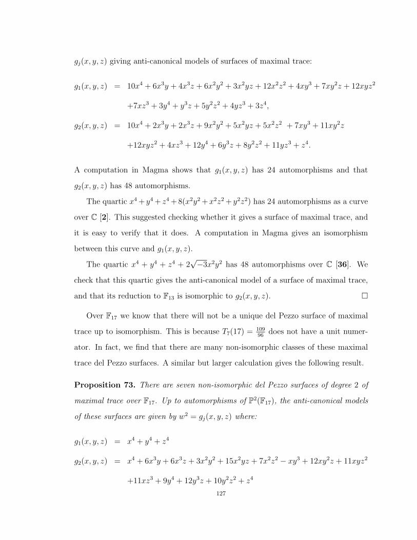
gj(x, y, z) giving anti-canonical models of surfaces of maximal trace:

g1(x, y, z) = 10x4 + 6x3y + 4x3z + 6x2y2 + 3x2yz + 12x2z2 + 4xy3 + 7xy2z + 12xyz2

+7xz3 + 3y4 + y3z + 5y2z2 + 4yz3 + 3z4,

g2(x, y, z) = 10x4 + 2x3y + 2x3z + 9x2y2 + 5x2yz + 5x2z2 + 7xy3 + 11xy2z

+12xyz2 + 4xz3 + 12y4 + 6y3z + 8y2z2 + 11yz3 + z4.

A computation in Magma shows that g1(x, y, z) has 24 automorphisms and that

g2(x, y, z) has 48 automorphisms.

The quartic x4 + y4 + z4 + 8(x2y2 +x2z2 + y2z2) has 24 automorphisms as a curve

over C [2]. This suggested checking whether it gives a surface of maximal trace, and

it is easy to verify that it does. A computation in Magma gives an isomorphism

between this curve and g1(x, y, z).

The quartic x4 + y4 + z4 + 2√−3x2y2 has 48 automorphisms over C [36]. We

check that this quartic gives the anti-canonical model of a surface of maximal trace,

and that its reduction to F13 is isomorphic to g2(x, y, z).

Over F17 we know that there will not be a unique del Pezzo surface of maximal

trace up to isomorphism. This is because T7(17) = 10996

does not have a unit numer-

ator. In fact, we find that there are many non-isomorphic classes of these maximal

trace del Pezzo surfaces. A similar but larger calculation gives the following result.

Proposition 73. There are seven non-isomorphic del Pezzo surfaces of degree 2 of

maximal trace over F17. Up to automorphisms of P2(F17), the anti-canonical models

of these surfaces are given by w2 = gj(x, y, z) where:

g1(x, y, z) = x4 + y4 + z4

g2(x, y, z) = x4 + 6x3y + 6x3z + 3x2y2 + 15x2yz + 7x2z2 − xy3 + 12xy2z + 11xyz2

+11xz3 + 9y4 + 12y3z + 10y2z2 + z4

127

g3(x, y, z) = x4 + 10x3y + 16x2y2 + 5x2yz + 14x2z2 + 6xy3 + 16xy2z + 4xyz2 − y4

+14y3z + 14y2z2 + yz3 + 15z4

g4(x, y, z) = 2x4 + 9x3y + 5x3z + x2y2 + 6x2yz + 16x2z2 + 14xy3 + 6xy2z

+14xyz2 + 6xz3 + 4y4 + 5y3z + 5y2z2 + 9yz3 + 9z4

g5(x, y, z) = 15x4 + 16x3y + 14x3z + 6x2y2 + 9x2yz + 13x2z2 + xy3 + 16xy2z

+16xyz2 + 9xz3 + 15y4 + 3y3z + 13y2z2 + 8yz3 + 16z4

g6(x, y, z) = 9x4 + 9x3y + x3z + 8x2y2 + 2x2yz + 5x2z2 + 5xy3 + 8xy2z + 13xyz2

+13xz3 + 16y4 + 4y3z + 15y2z2 + 7yz3 + 8z4

g7(x, y, z) = 13x4 + 12x3y + 13x3z + 11x2y2 + 12x2yz + 2x2z2 + 4xy3 + 5xy2z

+2xyz2 + 10xz3 + 9y4 + 14y3z + 13y2z2 + 9yz3 + 9z4.

The quartics gj(x, y, z) have 96, 24, 24, 8, 6, 4, and 2 automorphisms, respectively.

We compute

T7(17) =1

96+

2

24+

1

8+

1

6+

1

4+

1

2.

We also note that we first found a different model of the curve with 96 automorphisms.

A calculation shows that it is isomorphic to the Fermat quartic. We could similarly

try to find a nicer model of the curves of 24 automorphisms, for example, but have

not.

We note that T7(q) grows like a constant times q6. It is an easy calculation to see

that it is increasing for all q ≥ 7 and that it is greater than 1 for all q ≥ 13.

Proposition 74. The only finite fields Fq of odd characteristic for which there is a

unique degree 2 del Pezzo surface of maximal trace are F9 and F13.

128

In fact, the number of isomorphism classes of surfaces of maximal trace grows

quickly. The generic genus 3 curve has no non-trivial automorphisms, so as q →∞,

we expect a constant times q6 isomorphism classes of surfaces of maximal trace.

A more extensive calculation gives the classification of degree 2 del Pezzo surfaces

of maximal trace over F19.

Proposition 75. There are 14 non-isomorphic maximal del Pezzo surfaces of degree

2 over F19. Up to automorphisms of P2(F19), the anti-canonical models of these

surfaces are given by w2 = gj(x, y, z) where:

g1(x, y, z) = 16x4 + 9x3y + 10x3z + 11x2y2 + 14x2yz + 9xy3 + 4xyz2 + 3xz3

+16y4 + 4y3z + 17y2z2 + 17yz3 + 6z4

g2(x, y, z) = 9x4 + 4x3y + 9x3z + 18x2y2 + 10x2yz + 5x2z2 + 10xy3 + 9xy2z

+2xyz2 + 18xz3 + 4y4 + 9y3z + 8y2z2 + 15yz3 + 17z4

g3(x, y, z) = 11x4 + 15x3y + 11x3z + 6x2y2 + 12x2yz + 4x2z2 + 4xy3

+2xy2z + 18xyz2 + 3xz3 + 11y4 + 16y3z + 16y2z2 + 5yz3 + 6z4

g4(x, y, z) = 4x4 + 15x3y + 13x3z + 13x2y2 + 3x2yz + 16x2z2 + 13xy3

+10xy2z + 4xyz2 + 17xz3 + 9y4 + 15y3z + 5y2z2 + 5yz3 + 11z4

g5(x, y, z) = 7x4 + 5x3y + 17x3z + x2y2 + 11x2yz + x2z2 + 6xy3 + 10xy2z

+5xyz2 + 15xz3 + 4y4 + 4y3z + 7y2z2 + 10yz3 + 9z4

g6(x, y, z) = 9x4 + 13x3y + 5x3z + 13x2y2 + 12x2yz + 8x2z2 + 15xy3

+10xy2z + 7xyz2 + 2xz3 + 4y4 + 2y3z + 7y2z2 + 15yz3 + 6z4

g7(x, y, z) = 5x4 + 4x3y + 17x3z + 14x2y2 + 11x2yz + 14x2z2 + 3xy3

+6xy2z + 13xyz2 + 17xz3 + 4y4 + 8y3z + 18y2z2 + 14yz3 + 5z4

129

g8(x, y, z) = 6x4 + 3x3z + 5x2y2 + 8x2yz + 10x2z2 + 18xy2z + 6xyz2

+3xz3 + 5y4 + 16y3z + 12y2z2 + yz3 + 6z4

g9(x, y, z) = 9x4 + 14x3y + 11x3z + 11x2y2 + 16x2yz + 12x2z2 + 13xy3

+9xy2z + 14xyz2 + 10xz3 + 16y4 + 7y3z + 14y2z2 + 4yz3 + z4

g10(x, y, z) = 16x4 + 14x3y + 12x3z + 16x2yz + 5x2z2 + 2xy3 + 16xy2z

+9xyz2 + 4xz3 + 17y4 + 15y3z + 6y2z2 + 11yz3 + 6z4

g11(x, y, z) = x4 + 7x3y + 15x3z + 13x2y2 + 2x2yz + 8x2z2 + 5xy3 + 6xy2z

+5xyz2 + 11xz3 + 4y4 + 4y3z + 15y2z2 + 4z4

g12(x, y, z) = x4 + 17x3y + 5x3z + 2x2y2 + 6x2yz + 16x2z2 + 18xy3 + 10xy2z

+16xyz2 + 3xz3 + 5y4 + 2y2z2 + 11yz3 + 11z4

g13(x, y, z) = 7x4 + x3y + 6x3z + 4x2yz + 15x2z2 + 11xy3 + 11xy2z

+6xyz2 + 2xz3 + 11y4 + 9y2z2 + 11yz3 + 5z4

g14(x, y, z) = 16x4 + 2x3y + 10x3z + 16x2y2 + 8x2yz + 5x2z2 + 3xy3

+18xy2z + 17xyz2 + xz3 + 17y4 + 14y3z + y2z2 + 5yz3 + 7z4.

A computation shows that the first four quartics, gj(x, y, z), have 2 automorphisms

each, the next has 4, the next two have 6, the next three have 8, the next one has 9,

and the final three have 24 each.

We note that

T7(19) =115

36=

4

2+

1

4+

2

6+

3

8+

1

9+

3

24,

so these quartics account for all surfaces of maximal trace. This is the last case in

which we intend to completely classify the del Pezzo surfaces of degree 2 of maximal

trace. For F23 we first see a quartic f4(x, y, z) with trivial automorphism group such

130

that w2 = f4(x, y, z) is the anti-canonical model of a del Pezzo surface of maximal

trace.

Proposition 76. There are at least 19 distinct isomorphism classes of degree 2 del

Pezzo surfaces of maximal trace over F23. The equations w2 = gj(x, y, z) where

g1(x, y, z) = 18x4 + 18x3y + 11x3z + 9x2y2 + 11x2yz + 4x2z2 + 8xy3

+13xy2z + 2xyz2 + 7xz3 + y4 + 8y2z2 + 11yz3 + 9z4,

g2(x, y, z) = 4x4 + x3y + 12x3z + 7x2y2 + 10x2yz + 8x2z2 + 5xy3 + 18xy2z

+16xyz2 + 10xz3 + 8y4 + 19y3z + 4y2z2 + 5yz3 + 13z4,

are anti-canonical models of surfaces of maximal trace. Each of these quartics has

no non-trivial automorphisms.

Proof. Computation shows that T7(23) = 46128

= 16 + 1328

. It takes at least 19

unit fractions to reach this sum. The two quartics in the proposition statement come

from carrying out the process described above starting with a 7-tuple of points of

P2(F23) in general position.

We now turn to a different aspect of these counts. By studying congruence prop-

erties of the sextic polynomial in the numerator of T7(q) we can show that over

certain fields Fq there must exist a maximal trace surface with anti-canonical model

w2 = f4(x, y, z), where f4(x, y, z) has an automorphism of given order.

Proposition 77. Suppose that q is an odd prime power.

(1) If q ≡ 1, 2, 4 (mod 7) then there exists a quartic f4(x, y, z) with an automor-

phism of order 7 such that w2 = f4(x, y, z) is the anti-canonical model of a

del Pezzo surface of degree 2 of maximal trace.

131

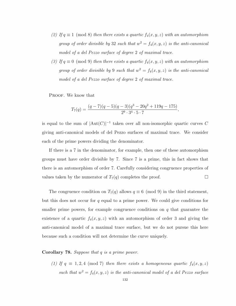
(2) If q ≡ 1 (mod 8) then there exists a quartic f4(x, y, z) with an automorphism

group of order divisible by 32 such that w2 = f4(x, y, z) is the anti-canonical

model of a del Pezzo surface of degree 2 of maximal trace.

(3) If q ≡ 0 (mod 9) then there exists a quartic f4(x, y, z) with an automorphism

group of order divisible by 9 such that w2 = f4(x, y, z) is the anti-canonical

model of a del Pezzo surface of degree 2 of maximal trace.

Proof. We know that

T7(q) =(q − 7)(q − 5)(q − 3)(q3 − 20q2 + 119q − 175)

29 · 34 · 5 · 7,

is equal to the sum of |Aut(C)|−1 taken over all non-isomorphic quartic curves C

giving anti-canonical models of del Pezzo surfaces of maximal trace. We consider

each of the prime powers dividing the denominator.

If there is a 7 in the denominator, for example, then one of these automorphism

groups must have order divisible by 7. Since 7 is a prime, this in fact shows that

there is an automorphism of order 7. Carefully considering congruence properties of

values taken by the numerator of T7(q) completes the proof.

The congruence condition on T7(q) allows q ≡ 6 (mod 9) in the third statement,

but this does not occur for q equal to a prime power. We could give conditions for

smaller prime powers, for example congruence conditions on q that guarantee the

existence of a quartic f4(x, y, z) with an automorphism of order 3 and giving the

anti-canonical model of a maximal trace surface, but we do not pursue this here

because such a condition will not determine the curve uniquely.

Corollary 78. Suppose that q is a prime power.

(1) If q ≡ 1, 2, 4 (mod 7) then there exists a homogeneous quartic f4(x, y, z)

such that w2 = f4(x, y, z) is the anti-canonical model of a del Pezzo surface

132

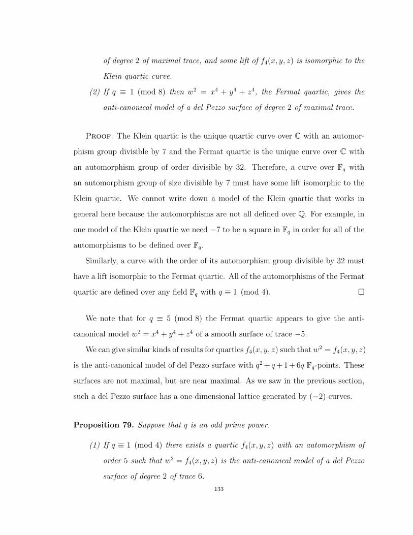
of degree 2 of maximal trace, and some lift of f4(x, y, z) is isomorphic to the

Klein quartic curve.

(2) If q ≡ 1 (mod 8) then w2 = x4 + y4 + z4, the Fermat quartic, gives the

anti-canonical model of a del Pezzo surface of degree 2 of maximal trace.

Proof. The Klein quartic is the unique quartic curve over C with an automor-

phism group divisible by 7 and the Fermat quartic is the unique curve over C with

an automorphism group of order divisible by 32. Therefore, a curve over Fq with

an automorphism group of size divisible by 7 must have some lift isomorphic to the

Klein quartic. We cannot write down a model of the Klein quartic that works in

general here because the automorphisms are not all defined over Q. For example, in

one model of the Klein quartic we need −7 to be a square in Fq in order for all of the

automorphisms to be defined over Fq.

Similarly, a curve with the order of its automorphism group divisible by 32 must

have a lift isomorphic to the Fermat quartic. All of the automorphisms of the Fermat

quartic are defined over any field Fq with q ≡ 1 (mod 4).

We note that for q ≡ 5 (mod 8) the Fermat quartic appears to give the anti-

canonical model w2 = x4 + y4 + z4 of a smooth surface of trace −5.

We can give similar kinds of results for quartics f4(x, y, z) such that w2 = f4(x, y, z)

is the anti-canonical model of del Pezzo surface with q2 + q+ 1 + 6q Fq-points. These

surfaces are not maximal, but are near maximal. As we saw in the previous section,

such a del Pezzo surface has a one-dimensional lattice generated by (−2)-curves.

Proposition 79. Suppose that q is an odd prime power.

(1) If q ≡ 1 (mod 4) there exists a quartic f4(x, y, z) with an automorphism of

order 5 such that w2 = f4(x, y, z) is the anti-canonical model of a del Pezzo

surface of degree 2 of trace 6.

133

(2) If q ≡ 1 (mod 8) there exists a quartic f4(x, y, z) with an automorphism

group of order divisible by 16 such that w2 = f4(x, y, z) is the anti-canonical

model of a del Pezzo surface of degree 2 with trace 6.

(3) If q ≡ 1, 2, 4, 8 (mod 9) there exists a quartic f4(x, y, z) with an automor-

phism of order 3 such that w2 = f4(x, y, z) is the anti-canonical model of a

del Pezzo surface of degree 2 with trace 6.

It will be useful for this proof and in the arguments that follow to define the

analogue of T7(q) for trace 6 surfaces. Let

T6(q) =(q − 7)(q − 5)(q − 3)(q3 − 20q2 + 119q − 175)

28 · 32 · 5.

This is a62

|W (E7)| divided by |GL3(Fq)|. Just as T7(q) is the sum of |Aut(C)|−1 over

all non-isomorphic curves f4(x, y, z) with w2 = f4(x, y, z) the anti-canonical model of

a surface of maximal trace, T6(q) is this sum over all non-isomorphic curves C giving

the anti-canonical model of a surface of trace 6.

Proof. We consider the prime factors that occur in the denominator of T6(q).

Studying congruence properties of the quintic in the numerator shows that there is

a factor of 5 in the denominator of T6(q) exactly when q ≡ 1 (mod 4). Similarly, the

denominator of T6(q) is divisible by 16 when q ≡ 1 (mod 8), and is divisible by 3

when q ≡ 1, 2, 4, 8 (mod 9).

We can also go through a similar analysis to the one used above for surfaces of

maximal trace in order to study del Pezzo surfaces of near-maximal trace.

Proposition 80. There is a unique del Pezzo surface of degree 2 of trace 6 over F9.

Up to automorphisms of P2(F9), its anti-canonical model is given by the homogeneous

quartic w2 = x4 − y4 + xyz2.

Proof. We compute T6(q) = 116

. We found this quartic by starting with a 7-tuple

of points in P2(Fq) in near general position and following the procedure to produce

134

an equation of the form w2 = f4(x, y, z) described above. We get the quartic

f4(x, y, z) = 2ax3y + (2a+ 1)x2y2 + 2x2yz + (a+ 1)xy3 + (2a+ 1)xy2z

+(a+ 1)xyz2 + (2a+ 2)y3z + (a+ 1)y2z2 + x4 + (a+ 1)y4.

We note that this curve has a unique singular point at [x : y : z] = [0 : 0 : 1], since the

z4, xz3 and yz3 coefficients of this curve are 0. Some convenient changes of variables

give us the form described in the statement.

It is no longer so straightforward to compute the size of the automorphism group

of this curve. Magma does not return the size of the automorphism group of a

singular curve, but of the normalization of the curve. In this case, the normalization

has 48 automorphisms. However, with our nicer model it is possible to determine the

automorphism group directly. We omit the details of this computation.

We could continue this kind of analysis like we did above for maximal trace

surfaces. We compute T6(11) = 3760

, so it is already clear that there is not a unique

surface of trace 6. For q ≥ 13 we see that T6(q) > 1, so it is not possible for there to

be a unique surface of trace 6.

Proposition 81. The only finite field of odd characteristic for which there is a unique

degree 2 del Pezzo surface of trace 6 is F9.

We now turn to the values of q for which Fq does not have characteristic 2 or 3,

and there are no del Pezzo surfaces of trace 6 or 7. These are q = 5 and q = 7.

Proposition 82. There is a unique del Pezzo surface of degree 2 over F5 of trace 5.

Up to automorphisms of P2(F5), its anti-canonical model is w2 = 2(x4 + y4 + z4).

Proof. By Theorem 3 that there are 7750 equations of the form w2 = f4(x, y, z)

that are anti-canonical models of a del Pezzo surface of degree 2 of trace 5. It

is not hard to verify that f4(x, y, z) = 2(x4 + y4 + z4) gives one such surface and

135

that f4(x, y, z) is smooth. This curve has 96 automorphisms. Therefore, this curve

contributes

|GL3(F5)|2 · 96

= 7750

equations to the total count.

The analogous count for surfaces of trace 5 over F7 is 10557540. Multiplying by

2|GL3(F7)| gives 5

8. Therefore, it is not possible that there is a unique smooth surface

of trace 5 over F7.

4. Dual Code Coefficients from del Pezzo Surfaces of Degree 2

In this section we prove Theorems 63 and 64. The main idea is to determine the

possible supports of a codeword of weight at most 10 of C′⊥2,4 and of Cc⊥

2,4 and then to

find the number of codewords with given type of support by polynomial interpolation.

Recall that these codes have length q3 + q2 + q corresponding to the nonsingular

points of P(2, 1, 1, 1) with coordinates [w : x : y : z]. The standard affine representa-

tives for P2(Fq) are the points (1, a, b), (0, 1, a), (0, 0, 1), where a, b ∈ Fq. We choose

affine representatives for the nonsingular points of P(2, 1, 1, 1) given by (w, p) where

w ∈ Fq and p is one of these standard affine representatives for P2(Fq). We think

of each point p as having q values of w lying above it, giving q points (w, p) where

w ∈ Fq.

Suppose c is a codeword of C′⊥2,4 of weight k with with nonzero coordinates

a1, . . . , ak corresponding to the points (w1, p1), (w2, p2), . . . , (wk, pk). These points

are called the support of c. It will be important for us to consider the multiset given

by the projection to P2(Fq), p1, . . . , pk. This is a multiset that does not have to

be a set because there can be distinct points (wi1 , pi) and (wi2 , pi) in the support of

a codeword. We have

αk∑i=1

aiw2i +

k∑i=1

aif4(pi) = 0,

136

for all α ∈ Fq and all homogeneous quartics f4(x, y, z). The only difference if c is a

codeword of Cc⊥2,4 is that we need only consider α = 0. In this case, it is clear that

once the multiset p1, . . . pk is fixed, we need only choose the values of wi so that

the points of the support are distinct.

It is only possible for this equality to hold for all homogeneous quartics of the

form αw2 − f4(x, y, z) if both sums are zero. Suppose that this is not the case. Then

there is a collection of points (w1, p1), . . . , (wk, pk) and some collection of coefficients

a1, . . . , ak for which the first sum α∑k

i=1 aiw2i is nonzero but

α

k∑i=1

aiw2i +

k∑i=1

aif4(pi) = 0,

for all α and f4(x, y, z). Taking α = 0 shows that this is not possible.

We consider the two sums separately. Let p′1, . . . , p′r be a maximal subset of

distinct elements of p1, . . . , pk. Then

k∑i=1

aif4(pi) =r∑j=1

a′jf(p′j) = 0,

where the a′j are expressed as sums of the ai. We focus on the subset of the a′j that are

nonzero. Call this set b1, . . . , bm and the corresponding points p′′1, . . . , p′′m. This

set defines a codeword of weight m ≤ r of C⊥2,4. The following result, Proposition 1

in [19], narrows down the possibilities for the set p′′1, . . . , p′′m. This result is a step

in the direction of the Cayley-Bacharach theorem.

Proposition 83. Let Ω = p1, . . . , pn ⊂ P2 be any collection of n ≤ 2d+ 2 distinct

points. The points of Ω fail to impose independent conditions on curves of degree d

if and only if either d + 2 of the points of Ω are collinear or n = 2d + 2 and Ω is

contained in a conic.

We apply this to the case d = 4 and conclude that if k ≤ 10 points fail to impose

independent conditions on homogeneous quartics then either 6 points lie on a line or

137

k = 10 and these points are contained in a conic. In the case of 10 points, either 6

points lie on a line, all 10 points lie on a smooth conic, or the 10 points lie on a conic

given as the union of two lines, exactly 5 points on each.

Corollary 84. Either the set p′′1, . . . , p′′m consists of m collinear points, or m = 10

and this set is contained in a smooth conic, or is contained in two lines, exactly 5

points on each.

Proof. Suppose this is not the case. By the previous proposition, the set

p′′1, . . . , p′′m contains 6 points on some line L and at least one point not on L.

Consider such a configuration that has the minimal number of collinear points. We

rearrange these points so that p′′1, . . . , p′′l is this set of collinear points. We see that

l ≥ 6. Without loss of generality suppose p′′m is not on L.

Consider any dual codeword with support p′′1, . . . , p′′m and nonzero coordinates

b1, . . . , bm with each bi 6= 0. For any 6 collinear points, for example p′′1, . . . , p′′6, there

is a dual codeword supported on these points with coefficients c1, . . . , c6. Subtracting

the appropriate scalar multiple of this codeword gives a dual codeword with the

coordinate corresponding to p′′1 equal to 0. The support of this codeword is contained

in p′′2, . . . , p′′m. The number of collinear points of the support of this codeword is at

most l − 1, contradicting the above assumption.

This gives a complete description of the possible supports of a codeword of weight

at most 10 of C⊥2,4. We now return to the dual codewords of weight at most 10 of C′⊥2,4

and Cc⊥2,4.

Proposition 85. Let c be a codeword of weight at most 10 of either C′⊥2,4 or Cc⊥

2,4 with

support (w1, p1), . . . , (wk, pk). Let p′1, . . . , p′r be the underlying set of points pi.

(1) If k ≤ 9 then the set p′1, . . . , p′r either consists of at most four points, or is

contained in a line together with one point not on the line.

138

(2) If k = 10 and r < 10 then the set p′1, . . . , p′r either consists of at most five

points, or is contained in a line together with two points not on the line.

(3) If k = 10 and r = 10 then the set p′1, . . . , p′10 either consists of ten points

on a line, ten points on a smooth conic, or ten points contained in two lines,

exactly five points on each.

Proof. Suppose c has nonzero coordinates a1, . . . , ak corresponding to the points

of its support. For each p′i ∈ p′1, . . . , p′r let a′i be the sum of aj for all points of the

support (wj, pj) with pj = p′i. Let b1, . . . , bm be the multiset of a′i that are nonzero

and let p′′1, . . . , p′′m be the corresponding set of points. As above, the coordinates

b1, . . . , bm determine an element of C⊥2,4 of weight m. The third statement follows

directly from Corollary 84. That result also shows that if m < 10 then the points

p′′1, . . . , p′′m are collinear.

Suppose pj is such that (wj1 , pj), . . . , (wjl , pj) are points of the support of c with

nonzero coordinates aj1 , . . . , ajl . Then

l∑i=1

ajif4(pj) = 0

implies that∑l

i=1 aji = 0. Therefore, l ≥ 2. It is possible to have l = 2 since

af4(p′j) + (−a)f4(p′j) = 0 for all f4(x, y, z). Therefore, the set p′1, . . . , p′r consists of

m ≥ 6 collinear points together with at most b r−m2c other points.

This result classifies the sets p′1, . . . , p′r that occur for a dual codeword of weight

at most 10. The next goal is to count the number of codewords that have a spe-

cific type of underlying set. For weight at most 7 it is not so difficult to give ex-

plicit formulas the number of codewords with each possible type of underlying set

p′1, . . . , p′r, but for weights 8, 9, and 10 the counts become very intricate. We de-

termine these counts by showing that for each weight k ≤ 10 and each possible type

of set p′1, . . . , p′r, the number of codewords of C′⊥2,4 and of Cc⊥

2,4 of weight k with

139

this type of underlying set is given by a polynomial in q, with a single exception.

The count for weight 10 codewords of C′⊥2,4 where p′1, . . . , p′r are 10 points on a line

involves τ(q). We consider this case separately.

We recall the definition of a code restricted to a subset. For a code C over FNq and

a set i1, . . . , ik ⊆ [1, N ], the code C restricted to this set is the image of the map

taking c = (c1, . . . , cN) to c′ ∈ FN−kq where all of the coordinates except ci1 , . . . , cik

are omitted. This map is not necessarily injective. In this case, C restricted to this

set is actually a multiset of codewords.

Lemma 86. Let C ′ denote either the code C ′2,4 or the code Cc2,4. Let

S := (w1, p1), . . . , (wk, pk)

denote a subset of distinct points of P(2, 1, 1, 1). Let C ′|S denote the code C ′ restricted

to the coordinates corresponding to points of S. The number of codewords of C ′⊥ of

weight r supported on S is given by the Xk−rY r coefficient of

1

|C ′|WC′|S(X + (q − 1)Y,X − Y ).

Proof. This is a straightforward application of the MacWilliams theorem and

the definition of a dual code coefficient of a code that comes from evaluating polyno-

mials. When the set S is small it is possible that codewords corresponding to distinct

polynomials can be equal, that is, the kernel of the map taking a polynomial to an

element of Fkq is non-trivial. In this case the size of the kernel is cancelled by the

appropriate factor of |C ′|−1.

As an example, we determine the number of codewords of weight at most 10 of

Cc⊥2,4 supported on the q points (w, p1), where p1 is fixed and w ∈ Fq. Such a codeword

has underlying set p′1, . . . , p′r = p1 in the notation defined above. It is clear that

there are no such codewords of weight 1.

140

Suppose that c is a codeword of weight 2 with support (w1, p1) and (w2, p1) and

nonzero coordinates a1 and a2. By definition w1 6= w2 and a1f4(p1) + a2f4(p1) = 0

for all homogeneous quartics f4(x, y, z). Therefore, a2 = −a1. This gives q − 1 such

codewords. We check that this matches the computation from the previous lemma.

There are q15 homogeneous quartics f4(x, y, z) and q14 of them vanish at a given

point p1. This gives

WC′|S(X, Y ) = q14X2 + (q15 − q14)Y 2.

Therefore

1

q15WC′|S(X + (q − 1)Y,X − Y ) =

1

q2

(q(X + (q − 1)Y )2 + (q2 − q)(X − Y )2

)= X2 + (q − 1)Y 2,

for the set S consisting of these two chosen points.

We can similarly count the number of such codewords where w1 and w2 are allowed

to vary. This multiplies the previous count by q(q−1)2

, which we could also see from

the weight enumerator of the punctured code. We have

1

q15WC′|S(X + (q − 1)Y,X − Y ) =

1

q((X + (q − 1)Y )q + (q − 1)(X − Y )q)

= Xq +(q − 1)2q

2Xq−2Y 2 +

(q − 1)2(q − 2)2q

6Xq−3Y 3 +O(Y 4).

For a weight k codeword supported on points of the form (w, p1) the k values of

wi can be chosen arbitrarily as long as they are distinct, and the nonzero coordinates

ai can be chosen arbitrarily as long as they sum to 0. It is clear that for all k the

number of codewords of this type is a polynomial in q.

We now investigate the codewords supported on points of the form (w, p1) of

C′⊥2,4. A weight k codeword still comes from choosing the nonzero coordinates ai that

141

sum to 0, but there is now the additional condition that∑k

i=1 aiw2i = 0. We have

ak = −(a1 + · · ·+ ak−1).

We first choose k distinct values w1, . . . , wk. The goal is to count solutions to

a1(w21 − w2

k) + a2(w22 − w2

k) + · · ·+ ak−1(w2k−1 − w2

k) = 0,

such that each ai is nonzero. Since wj 6= wk for j 6= k the only way for w2j − w2

k = 0

is for wj = −wk. We see that this can hold for at most one value of j ∈ [1, k − 1].

We consider two cases based on whether there is a term w2j − w2

k = 0 for some

j < k. We claim that in each case the number of solutions with each ai 6= 0 is given

by a polynomial in q. We prove this by induction on k. This holds for k = 1 where

we note that all solutions correspond to the case where w21 − w2

2 = 0. Suppose this

holds for all k ≤ m− 1.

First suppose that there is some j < m for which w2j − w2

k = 0. Without loss of

generality, suppose that w21−w2

k = 0. Then a1 can be any nonzero element of F∗q and

a2(w22 − w2

m) + · · ·+ am−1(w2m−1 − w2

m) = 0,

where each w2j − w2

m 6= 0. By induction, the number of such solutions a1, . . . , am−1

with each aj nonzero is given by a polynomial in q.

We now consider the case where each w2j − w2

k 6= 0. There are qk−2 solutions

a1, . . . , ak−1, but we only want to count the ones for which each ai 6= 0. By letting

a′i = ai(w2i −w2

k)−1, we see that this does not depend on the choice of w1, . . . , wk. We

need only note that for each k, the number of solutions of a1 + · · ·+ ak−1 = 0 where

each ai is nonzero is given by a polynomial in q. We summarize this below.

Lemma 87. For each k ≤ 10, the number of codewords of weight k of C′⊥2,4 that are

supported on points of the form (w, p1) where w ∈ Fq and p1 is fixed, is given by a

polynomial in q.

142

We can find these polynomials explicitly by Lagrange interpolation. We note that

the number of codewords of weight k is bounded by q2k, the number of possibilities

for the nonzero coordinates a1, . . . , ak times the number of possibilities of the points

(w1, p1), . . . , (wk, p1).

Corollary 88. The contribution to the weight enumerator of C′⊥2,4 from codewords of

weight at most 10 that are supported on points of the form (w, p1) where w ∈ Fq and

p1 is fixed, is given by

(q − 1)2

10∑j=2

Aj(q)

j!Xq3+q2+q−jY j,

where the Aj(q) are given by:

A2(q) = 1 A3(q) = (q − 3)(q − 2)

A4(q) = (q − 3)(q − 2)(q2 − 3 q + 6

)A5(q) = (q − 4)(q − 3)(q − 2)

(q3 − 4 q2 + 6 q − 10

)A6(q) = (q − 5)(q − 4)(q − 3)(q − 2)

(q4 − 5 q3 + 10 q2 − 10 q + 15

)A7(q) = (q − 6)(q − 5)(q − 4)(q − 3)(q − 2)

(q5 − 6 q4 + 15 q3 − 20 q2 + 15 q − 21

)A8(q) = (q − 7) (q − 6)(q − 5) (q − 4) (q − 3)(q − 2)

(q6 − 7 q5 + 21 q4 − 35 q3

+35 q2 − 21 q + 28

)A9(q) = (q − 8)(q − 7)(q − 6)(q − 5)(q − 4)(q − 3) (q − 2)

×(q7 − 8 q6 + 28 q5 − 56 q4 + 70 q3 − 56 q2 + 28 q − 36

)A10(q) = (q − 9)(q − 8)(q − 7)(q − 6)(q − 5)(q − 4)(q − 3)(q − 2)

×(q8 − 9 q7 + 36 q6 − 84 q5 + 126 q4 − 126 q3 + 84 q2 − 36 q + 45

).

Allowing different choices of p1 multiplies this expression by q2 + q + 1.

143

It is easy to give a similar result for Cc⊥2,4 but we do not exhibit it here.

The same argument gives a similar statement for dual codewords c of either C′⊥2,4 or

Cc⊥2,4 of weight at most 10 supported on the 5q points of the form (w, p1), . . . , (w, p5),

where each pi is fixed and w ∈ Fq is allowed to vary. Such a codeword of weight

k ≤ 10 with nonzero coordinates a1, . . . , ak satisfies

k∑i=1

aif4(pi) = 0,

for all homogeneous quartics f4(x, y, z). By Corollary 84, for each j ∈ [1, 5] the sum

of the ai taken over all i such that pi = pj is zero. For C′⊥2,4 the inclusion-exclusion

needed to determine these counts exactly becomes complicated, but the arguments

given above show the following. We note that there are(q2+q+1

k

)ways to choose k

points in P2(Fq), and this is a polynomial in q of degree 2k.

Proposition 89. Let C ′ denote the code C ′2,4 or Cc2,4. The number of codewords of

C ′⊥ of weight k ≤ 10 with support (w1, p1), . . . , (w10, p10) such that the multiset

p1, . . . , p10 contains at most 5 distinct points is given by a polynomial in q of degree

at most 4k.

Using this result and inclusion-exclusion it is possible to find for each k ≤ 10 and

for each j satisfying 1 ≤ j ≤ 5 the number of such codewords of weight k such that

p1, . . . , p10 contains exactly j distinct points. For example, the number of weight

10 codewords of C′⊥2,4 such that the set p1, . . . , p10 contains exactly 5 distinct points

is (q2 + q + 1

5

)(q − 1)10q4

32.

The initial factor comes from choosing 5 points in P2(Fq) and the rest comes from

counting codewords supported on 5 chosen points.

We next turn to one of the more complicated types of support described in Corol-

lary 84, namely 10 points on a smooth conic.

144

Proposition 90. The number of codewords of C⊥2,4 of weight 10 supported on a given

smooth conic is (q − 1)(q+110

).

Proof. We claim that given any 10 points on a smooth conic there is a unique

dual codeword supported on these points up to scalar multiplication. The count

is given by q − 1 times the number of collections of 10 points on a smooth conic.

By Bezout’s theorem a quartic intersecting a given conic at 9 points p1, . . . , p9 must

contain that conic. Given such a collection and any additional point of the conic p10

we can express

f4(p10) =9∑i=1

aif4(pi),

for a unique linear combination a1, . . . , a9, completing the proof.

Lemma 91. Suppose that c is a weight 10 codeword of C⊥2,4 supported on a smooth

conic. Then the product of the nonzero coordinates of c is −1 times a nonzero square

in F∗q.

We recall that a diagonal quadric in Pm−1(Fq) defines a plus quadric if the product

of the diagonal coefficients takes the same value that (−1)m2 does under the quadratic

character on F∗q. This follows directly from taking the product of the relevant Gauss

sums. This lemma gives exactly the condition required for a diagonal form in 10

variables with these coefficients to define a smooth plus quadric in P9(Fq).

Proof. A smooth conic has q+1 points so if q+1 < 10 there is nothing to prove.

For q = 9 we can verify this proposition directly by looking at the dual of the code of

quartics restricted to a particular smooth conic, say x2 + y2 + z2, using the fact that

PGL3(Fq) acts transitively on smooth conics. There is a unique codeword supported

on these ten points up to scalar multiplication. We can explicitly compute the linear

145

relation satisfied by these ten points

10∑i=1

aif4(pi) = 0,

for all quartic polynomials f4(x, y, z). In each case, the product of the ai is a square.

Now suppose that q > 9. A smooth conic is given by a quadratic embedding

[x2 : xy : y2] of P1(Fq) after a change of coordinates. A homogeneous quartic restricted

to this conic is just a homogeneous polynomial of degree 8 in x and y, the coordinates

of the original P1(Fq). Therefore, 10 points on this conic fail to impose independent

conditions on these quartics. The statement to be proven is equivalent to showing

that the product of the nonzero coordinates of a weight 10 codeword in the dual of

the code of homogeneous degree 8 polynomials on P1(Fq) takes the same value as −1

under the quadratic character.

Given 10 points p1, . . . , p10 on P1(Fq) we apply an automorphism of P1(Fq) so that

[1 : 0] is not one of these points. We dehomogenize and suppose that these points are

represented by x1, . . . , x10 in Fq. We define

Q(x) =10∏i=1

(x− xi), and Rjk(x) =Q(x)

(x− xj)(x− xk),

for each pair j, k satisfying 1 ≤ j < k ≤ 10. There is a linear relation among these

points

c1f(x1) + · · ·+ c10f(x10) = 0,

for all f(x) of degree at most 9. Let f(x) = Rjk(x). Note that Rjk(xk) 6= 0. Then

cjRjk(xj) + ckRjk(xk) = 0, and socjck

= (−1)Rjk(xj)

Rjk(xk).

We have10∏j=2

c1

cj=

c91

c2c3 · · · c10

= (−1)9

10∏i=2

R1i(x1)

R1i(xi).

146

Multiplying the left hand side by (c2 · · · c10)2 we see that it is a square times the

product c1c2 · · · c10. The right hand side is

(−1)

∏10i=2(xi − x1)8∏

2≤i<j≤10(xi − xj)(xj − xi).

This is −1 times (−1)(92) = 1 times a square, completing the proof.

Proposition 92. The number of weight 10 codewords of C′⊥2,4 that have support

(w1, p1), . . . , (w10, p10) such that p1, . . . , p10 are 10 distinct points on a smooth conic

in P2(Fq) is

(q − 1)(q5 − q2)

(q + 1

10

)(q9 + (q − 1)q4

).

The number of weight 10 codewords of Cc⊥2,4 with support (w1, p1), . . . , (w10, p10)

such that p1, . . . , p10 are 10 distinct points on a smooth conic in P2(Fq) is

(q − 1)(q5 − q2)

(q + 1

10

)q10.

Proof. The number of smooth conics in P2(Fq) is q5 − q2. The number of pos-

sibilities for p1, . . . , p10 lying on a particular smooth conic is given by Proposition

90.

By the previous lemma, if c is a weight 10 codeword of C′⊥2,4 that has support

(w1, p1), . . . , (w10, p10) with nonzero coordinates a1, . . . , a10 and p1, . . . , p10 satisfy-

ing the conditions of this proposition, then

10∑i=1

aiw2i = 0.

Since∏10

i=1 ai is −1 times a nonzero square,∑10

i=1 aix2i defines a plus quadric in

P9(Fq). Such a quadric has q9−1q−1

+ q4 Fq-rational points. Taking scalar multiples of

these projective points and adding in the possibility (w1, . . . , w10) = (0, . . . , 0) gives

q9 + (q − 1)q4 possibilities for (w1, . . . , w10).

147

If c is a weight 10 codeword of Cc⊥2,4 satisfying the conditions of this proposition

then there are q10 possibilities for (w1, . . . , w10).

Now suppose that c is a codeword of weight k ≤ 10 of C′⊥2,4 or of Cc⊥

2,4 that

has support (w1, p1), . . . , (wk, pk) and nonzero coordinates a1, . . . , ak. Consider the

multiset p1, . . . , pk and the underlying set p′1, . . . , p′r. Let a′j be the sum of the

ai such that pi = p′j. As we discussed above, some of the r values a′1, . . . , a′r may be

zero. Let b1, . . . , bm be the set that are nonzero. We have analyzed codewords with

p1, . . . , p10 lying on a smooth conic and codewords where each a′i = 0.

We now consider the case where the points p′1, . . . , p′r are collinear. We then

consider the case where we have a set of collinear points, and at most two other

points. Let L denote a fixed line in P2(Fq). For concreteness, we may suppose that

L is given by z = 0. Suppose we consider the code C ′2,4 punctured on all coordinates

except those corresponding to points (w, p), where w ∈ Fq and p ∈ L. This punctured

code has length q2 + q.

In Chapter 3 we studied the quadratic residue weight enumerator of the code

C1,4 with codewords corresponding to homogeneous quartics f4(x, y) on P1(Fq). We

determined QRC1,4(X, Y, Z) and studied the specialization QRC1,4

(X,X2, 1). This

latter polynomial tells us the distribution of point counts for the q5 homogeneous

quartics on P(2, 1, 1) of the form w2 − f4(x, y). This is the α = 1 part of the weight

enumerator of the six dimensional code of homogeneous quartics in the weighted

projective space P(2, 1, 1) given by equations of the form αw2 − f4(x, y). This is

very similar to the setup of the current problem. It is easy to write down the weight

enumerator of the 5-dimensional subcode given by α = 0, and we see that for each

k ≤ 10 the number of dual codewords of weight k is given by a polynomial in q.

We computed a homogenized version of the polynomial QRC1,4(X,X2, 1) and

then applied the classical MacWilliams theorem to it. Proposition 54 connected

this weight enumerator to the weight enumerator coming from the q5 homogeneous

148

quartics w2 = f4(x, y) on P(2, 1, 1). We note that the preimage in P(2, 1, 1, 1) of

a line in the [x : y : z] projective plane is a copy of P(2, 1, 1). After applying the

MacWilliams transformation to this weight enumerator of these q5 codewords we saw

that the Y 10 coefficient was a polynomial in q plus a polynomial in q times τ(q). For

each k satisfying 0 ≤ k ≤ 9, the Y k coefficient is given by a polynomial in q.

Proposition 93. The number of codewords c ∈ C′⊥2,4 of weight 10 with support

(w1, p1), . . . , (w10, p10) such that p1, . . . , p10 are distinct points on a line is equal

to P1(q) + P2(q) · τ(q), where P1(q), P2(q) are polynomials in q of degree at most 32.

Proof. This follows directly from Theorem 52 since the code coming from vari-

eties of the form w2 − f4(x, y, z) restricted to a line is equivalent to the code coming

from varieties of the form w2− f4(x, y). To make this more concrete, since PGL3(Fq)

acts transitively on lines we can choose the particular line given by z = 0.

The bound on the degree comes from the fact that there are at most (q + 1)10q10

possibilities of (w1, p1), . . . , (w10, p10) for a given line, at most (q − 1)10 choices of

nonzero coordinates (a1, . . . , a10), and exactly q2 + q + 1 lines.

Proposition 94. For each k ≤ 10, the number of codewords c ∈ Cc⊥2,4 of weight k with

support (w1, p1), . . . , (wk, pk) such that p1, . . . , pk are contained in a line is given by

a polynomial in q of degree at most 3k + 2.

For each k ≤ 9, the number of codewords c ∈ C′⊥2,4 of weight k with support

(w1, p1), . . . , (wk, pk) such that p1, . . . , pk are points in a line is given by a polyno-

mial in q of degree at most 3k + 2.

Proof. For the degree statement we note that there are at most (q + 1)kqk

possibilities of (w1, p1), . . . , (wk, pk) for a given line, at most (q − 1)k choices of

nonzero coordinates (a1, . . . , ak), and exactly q2+q+1 lines. The rest of the statement

follows from the discussion above.

149

As a corollary we state the contribution to the weight enumerator of C′⊥2,4 from

codewords of this type. We found this expression by computing the weight enumer-

ator of C ′2,4 restricted to the line z = 0 for many small values of q, applying the

MacWilliams theorem, and interpolating.

Corollary 95. The contribution to WC′⊥2,4

(X, Y ) from codewords that have support

(w1, p1), . . . , (wk, pk) such that p1, . . . , pk are contained in a line is given by

(q − 1)2(q + 1)(q2 + q + 1)10∑j=2

Aj(q)

j!Xq3+q2+q−jY j,

where the Aj(q) are:

A2(q) = 1, A3(q) = (q − 3)(q − 2)

A4(q) = ( q4 − 14 q3 + 30 q2 − 48 q + 36)

A5(q) = (q − 2)(11 q5 − 51 q4 + 96 q3 − 120 q2 + 142 q − 120

)A6(q) =

(q9 + 32 q8 − 317 q7 + 1292 q6 − 2979 q5 + 4390 q4 − 4646 q3 + 4195 q2 − 3510 q + 1800

)A7(q) = (q − 2)

(q11 + 3 q10 + 71 q9 − 1059 q8 + 5215 q7

−13904 q6 + 23381 q5 − 26593 q4 + 22530 q3 − 16467 q2 + 12582 q − 7560

)A8(q) = (q − 2)

(q14 + 3 q13 − 28 q12 + 212 q11 − 3633 q10 + 27323 q9 − 109335 q8 + 271198 q7

−449398 q6 + 521763 q5 − 442785 q4 + 301189 q3 − 190022 q2 + 130032 q − 70560

)A9(q) = (q − 2)

(q17 + 3 q16 − 37 q15 − 81 q14 + 1477 q13 − 14561 q12 + 124477 q11 − 681919 q10

+2401876 q9 − 5733040 q8 + 9629370 q7 − 11636558 q6 + 10325912 q5 − 6983436 q4 + 4000252 q3

−2277288 q2 + 1448352 q − 725760

)A10(q) =

(q21 + q20 − 53 q19 − 8 q18 + 1258 q17 + 1619 q16 − 78694 q15 + 744136 q14 − 5008985 q13

+24916147 q12 − 90514598 q11 + 242287029 q10 − 484799964 q9 + 732875889 q8 − 841222633 q7

+735105906 q6 − 494759040 q5 + 269674245 q4 − 136112652 q3 + 74629836 q2 − 42930000 q + 16329600)

−(q − 1)q5τ(q).

150

The term involving τ(q) exactly cancels with the term involving τ(q) coming from

WG1C′2,4

(X + (q − 1)Y,X − Y ). We can easily give a similar result for the contribution

to the weight enumerator of Cc⊥2,4, but do not write it here.

For small weight codewords we can explain the individual terms contributing

to this sum. For weight 8, 9, and 10 there are so many possibilities to consider

that it would be very difficult to write down this polynomial without some sort of

interpolation argument.

For example, we saw above that every codeword of weight 2 that has support

(w1, p), (w2, p) has nonzero coordinates a and −a. There are q+1 choices for p and

must choose w1 6= w2 satisfying aw21 − aw2

2 = 0. Since x21 − x2

2 = (x1 − x2)(x1 + x2),

we conclude w1 + w2 = 0. This gives (q + 1) (q−1)2

2such codewords.

A codeword of weight 3 has (w1, p), (w2, p), (w3, p) with nonzero coordinates

a, b,−(a + b). There are q + 1 choices of p and (q − 1)(q − 2) choices of a and b.

We must have aw21 + bw2

2 − (a + b)w23 = 0, where the wi are distinct. The equation

ax21 + bx2

2− (a+ b)x23 defines a smooth conic in P2(Fq), so it has q+ 1 rational points.

There are 4 additional points that we do not want to count because of the constraint

that the wi are distinct. These are the affine representatives of the projective points:

[1 : 1 : 1], [1 : 1 : −1], [1 : −1 : 1], [−1 : 1 : 1]. This gives (q−1)(q−3)6

choices for the

set w1, w2, w3, explaining the Y 3 coefficient.

For the Y 4 coefficient the support can either be (w1, p), (w2, p), (w3, p), (w4, p)

for some point p with the wi distinct, or can be (w1, p1), (w2, p1), (w3, p2), (w4, p2)

for some choice of p1 6= p2 where w1 6= w2 and w3 6= w4. We can determine the number

of codewords of each type and add them to get this term. We can do something very

similar for the weight 5 coefficient since there are still at most two distinct values of

p that occur.

For weight 6, things become a little more complicated. We consider the set of

(wi, pi) where 1 ≤ i ≤ 6. We can count codewords where exactly 1, 2, or 3 distinct

151

values of pi occur as above. However, it is possible now that all of the pi are distinct.

In this case,6∑i=1

aif4(pi) = 0 for all f4(x, y),

so these six points and the nonzero coordinates ai define a weight 6 codeword of

C⊥1,4. We have seen that any 6 points support a unique such codeword up to scalar

multiplication. Moreover, for such a codeword the product of the ai is a nonzero

square if q ≡ 1 (mod 4), and is a non-square if q ≡ 3 (mod 4). Therefore∑6

i=1 aix2i

defines a plus quadric in P5(Fq), which has exactly q4 + q3 + 2q2 + q + 1 Fq-points.

Taking scalar multiples and adding in the case where (w1, . . . , w6) = (0, . . . , 0) gives

q5 + (q − 1)q2. The number of codewords of this type is

(q − 1)

(q + 1

6

)(q5 + (q − 1)q2).

Adding these terms gives the weight 6 coefficient.

The weight 7 coefficient is the last case we analyze in complete detail. We deter-

mine the counts where 1, 2, or 3 distinct values of pi occur as above. We determine

the number of codewords such that the 7 values of pi are distinct using the number

of weight 7 codewords of C⊥1,4. The resulting quadric in P6(Fq) given by∑7

i=1 aix2i is

smooth, and all such quadrics have the same number of rational points.

The more complicated situation in where exactly 6 distinct points pi occur among

these 7 points and one occurs twice. For this repeated point there are two nonzero

coordinates a, b such that a + b 6= 0. Given a choice of 6 points there is a unique

codeword of C⊥1,4 supported on them. There are (q−1)(q−2)2

total choices of this pair

a, b. When considering the possibilities for (w1, . . . , w7) that lie on a smooth quadric

in P6(Fq) we must subtract the number of points for which the two w-values above

the point p occurring twice are equal. Restricting a smooth quadric to a hyperplane

xi = xj gives a smooth quadric in P5(Fq). Since the coefficients attached to the 6

distinct points that occur define a weight 6 codeword of C⊥1,4, this is a plus quadric

152

in P5(Fq). Taking scalar multiples gives an extra factor of q− 1. Therefore, the total

number of codewords of this form is

6

(q + 1

6

)(q − 1)(q − 2)

2(q− 1)2((q5 + q4 + q3 + q2 + q + 1)− (q4 + q3 + 2q2 + q + 1)).

Adding these terms gives the weight 7 term. We will not explain the weight 8, 9, and

10 coefficients in detail, but use the fact that the remaining terms are polynomials in

q to find them by interpolation. We checked these calculations well past the bound

on the degree of the resulting polynomials in order to get a check on the consistency

of the output.

We now turn to the next possibility for the support of a codeword of C′⊥2,4 or Cc⊥

2,4

of weight k ≤ 10. Suppose that such a codeword has support (w1, p1), . . . , (wk, pk)

such that p1, . . . pk is contained in a line together with two points, and has nonzero

coordinates a1, . . . , ak. Let p′1, . . . , p′r be the distinct values of pi that occur. For

each i satisfying 1 ≤ i ≤ r let a′i be the sum of the aj corresponding to points of

the support (wj, pj) satisfying pj = p′i. Consider the set b1, . . . , bm of these a′i that

are nonzero, and the corresponding set of points p′′1, . . . , p′′m. We see that this set

of p′′i must be contained in a line. In the case where this set is empty, it is easy to

count codewords of this type using the techniques described above. When this set is

not empty, the nonzero coordinates bi and the corresponding points give a weight m

codeword of C⊥1,4, so 6 ≤ m ≤ 10.

We have already analyzed the case where the set p1, . . . , pk is contained in a line

L. The only interesting case left is where this does not occur, when some elements of

this multiset of k points are equal to the two chosen points not lying on L. Let p′ be

one of these points not lying on L. In order for this c to give a dual codeword, the

sum of the nonzero coefficients for points (w, p) in the support of c with p = p′ must

be equal to zero. Therefore, we need only investigate a few new types of possible

supports of codewords.

153

We describe these codewords by describing the multiset p1, . . . , pk. The only

weight 8 codewords of this type have 6 distinct points on a line, and one point off the

line with two w-values above it. For weight 9 there are a few possibilities. There can

be 7 distinct points on the line and one point off the line that occurs twice. There

can also be 6 points on the line, one occurring twice, and a point off the line that

also occurs twice. Finally, there can be 6 points on the line each occurring once, and

one points off the line occurring three times.

For weight 10, we can have 6 points on the line each occurring once, and one point

off the line occurring four times. We can have 6 points on the line each occurring

once, and two distinct points off the line, each occurring twice. We can have 6 points

on the line, exactly one occurring twice, and one point off the line occurring three

times. We can have 6 points on the line, exactly two occurring twice, and one point

off the line occurring twice. We can have 6 points on the line, exactly one occurring

three times, and one point off the line occurring twice. We can have 7 distinct points

on the line each occurring once, and one point off the line occurring three times. We

can have 7 distinct points on the line exactly one occurring twice, and one point off

the line occurring twice. We can have 8 distinct points on the line each occurring

once, and one point off the line occurring twice.

Counting each such configuration is tedious, but the arguments given earlier in

this section imply the following. Again, this result is related to the analogous result

for P(2, 1, 1), Proposition 54.

Proposition 96. Let C ′ denote either the code C ′2,4 or Cc2,4. For each k ∈ [8, 10], the

number of weight k codewords of C ′⊥ with support (w1, p1), . . . , (wk, pk) such that

the underlying set p′1, . . . , p′r of the multiset p1, . . . , pk is not contained in a line

but is contained in a line together with two points, is given by a polynomial in q.

We go through a particular example in detail. Similar techniques can be used to

determine the counts for the other cases.

154

Suppose c ∈ C ′⊥2,4 has support (w1, p1), . . . , (w8, p8) with coefficients a1, . . . , a8

and that the multiset p1, . . . , p8 consists of 7 distinct points. Suppose that p1, . . . , p6

lie on a line and p7 = p8 is a point not on this line. So, w7 6= w8. Since a1, . . . , a6

gives a codeword of C′⊥2,4 of weight 6, the product of these coordinates is −1 times a

nonzero square in F∗q and∑6

i=1 aix2i defines a plus quadric in P5(Fq). Therefore,

a7w27 − a7w

28 +

6∑i=1

aiw2i

defines a plus quadric in P7(Fq) since the product of the coordinates is a nonzero

square in F∗q and (−1)7+12 = 1. Such a plus quadric has

∑6i=0 qi+q3 points. Multiply-

ing by q − 1 to account for scalar multiples and adding 1 for the solution (0, . . . , 0)

gives q7 + (q − 1)q3 solutions.

However, we must take into account the additional constraint that w7 6= w8. We

count the number of solutions that violate this condition. We see that (w1, . . . , w6)

must satisfy6∑i=1

aiw2i = 0,

the equation of a plus quadric in P5(Fq). Multiplying by q − 1 for scalar multiples

and by q to account for the value of w7 and then adding in the solutions where

(w1, . . . , w6) = (0, . . . 0) gives

q + q(q − 1)(q4 + q3 + 2q2 + q + 1) = q6 + q3(q − 1)

solutions. Subtracting gives q7 − q6 total possibilities for (w1, . . . , w8). We multiply

this by (q−1)(q+1

6

), the number of choices of a1, . . . , a6 and p1, . . . , p6, and by q2+q+1

to account for the number of choices of lines. We also have q2 choices of p7 not on

that line. In total this gives

(q2 + q + 1)q2(q − 1)

(q + 1

6

)q − 1

2(q7 − q6)

155

total dual codewords of weight 8 with support of this type. We could perform a

similar type of analysis for other possible supports, but it is enough for our purposes

to know that these counts are given by polynomials and then interpolate.

We now consider the final possibility for the support of a codeword.

Proposition 97. Let c ∈ C⊥2,4 be a codeword of weight 10 with support consisting of

exactly 5 points on each of two lines.

The number of such codewords is

(q − 1)(q2 + q + 1)(q + 1)q

2

(q

5

)2

.

Proof. The argument of Proposition 90 shows that any 10 points of a conic

fail to impose dependent conditions on quartics, but we also know that if there is

no subset of 6 collinear points then any subset of 9 of these points does impose

independent conditions. Therefore we need only count the number of collections of 5

points on each of two lines.

We first choose the point of intersection of these lines and then note that there

are (q+1)q2

pairs of lines intersecting at this point. For each of these two lines there

are(q5

)ways to choose 5 points not including the intersection point. Taking scalar

multiples gives an extra factor of q − 1. This completes the count.

Lemma 98. If c is a weight 10 codeword of C⊥2,4 supported on the union of two lines

then the product of the nonzero coordinates of c is −1 times a square in F∗q.

Proof. We let p1, . . . , p5 be the five points on the first line and q1, . . . , q5 be

the points of the second line. Let p′ be the point of intersection of these two lines. We

note that there is exactly one codeword supported on the points p1, . . . , p5, p′ up to

scalar multiplication, and exactly one supported on q1, . . . , q5, p′ up to scalar multi-

plication. Taking the appropriate scalar multiples so that the coefficients of p′ match,

the difference gives a dual codeword of weight 10 supported on p1, . . . , p5, q1, . . . , q5.

156

Taking all possible pairs of lines and collections of 5 points on each line satisfying

these conditions along with a choice of scalar multiple produces exactly the number

of codewords given in the previous proposition.

The product of the coefficients of the codeword c1 with support p1, . . . , p5, p′ is

always −1 times a nonzero square in F∗q, independent of the scalar multiple that we

take, and the same statement is true of the codeword c2 with support q1, . . . , q5, q′.

Now without loss of generality suppose the scalar multiples are chosen so that the p′

coefficient of each is 1. The product of the coefficients of c1 and c2 is a square. The

weight 10 codeword that we get from the difference c1− c2 is equal to the product of

the coefficients of p1, . . . , p5 in c1 times (−1)5 times the product of the coefficients of

q1, . . . , q5 in c2. This is a square divided by −1, since we have omitted the coefficient

of p′ in both c1 and −c2.

This lemma shows that such a codeword of weight 10 with nonzero coefficients

a1, . . . , a10 leads to a plus quadric in P9(Fq) given by∑10

i=1 aix2i = 0.

Proposition 99. The number of weight 10 codewords of C′⊥2,4 that have support

(w1, p1), . . . , (w10, p10) such that p1, . . . , p5 are distinct points on one line and

p6, . . . , p10 are distinct points on another line of P2(Fq) is

(q − 1)(q2 + q + 1)(q + 1)q

2

(q

5

)2

(q9 + (q − 1)q4).

The number of weight 10 codewords of Cc⊥2,4 with support (w1, p1), . . . , (w10, p10)

such that p1, . . . , p5 are distinct points on one line and p6, . . . , p10 are distinct

points on another line of P2(Fq) is

(q − 1)(q2 + q + 1)(q + 1)q

2

(q

5

)2

q10.

157

Proof. We first choose one of the q2 + q + 1 rational points of P2(Fq). The

number of pairs of Fq-rational lines through this point is (q+1)q2

. The number of ways

of choosing 5 points on each of these lines not including the intersection point is(q5

)2.

By the previous lemma, if c is a weight 10 codeword of C′⊥2,4 with support given

by (w1, p1), . . . , (w10, p10) satisfying the conditions of the proposition and nonzero

coordinates a1, . . . , a10, then10∑i=1

aiw2i = 0.

The previous lemma shows that∑10

i=1 aix2i defines a plus quadric in P9(Fq). Such a

quadric has q9−1q−1

+ q4 Fq-rational points. Taking scalar multiples of these projective

points and adding in the possibility (w1, . . . , w10) = (0, . . . , 0) gives q9 + (q − 1)q4

possibilities for (w1, . . . , w10).

If c is a weight 10 codeword of Cc⊥2,4 satisfying the conditions of this proposition

then there are q10 possibilities for (w1, . . . , w10).

Taking scalar multiples of these codewords gives an extra factor of q − 1.

Combining the counts for these different types of dual codewords is the final part

of the proof of Theorems 63 and 64.

Before moving on to the next topic, we briefly mention two directions for future

work. First, the main count given by Theorem 3 treats all anti-canonical models

of del Pezzo surfaces of degree 2 the same. It would be interesting to separate

the contribution coming from singular del Pezzo surfaces from the contribution of

the smooth surfaces. Said another way, it would be interesting to determine how

the trace of Frobenius acting on Pic(S) splits up as we vary over all homogeneous

quartics in P(2, 1, 1, 1) given by w2 = f4(x, y, z) where f4(x, y, z) is a smooth quartic

on P2(Fq), not just a quartic with at most simple singularities. This would require

some new extension of these ideas.

158

We have also seen that the Frobenius endomorphism induces a permutation of

the (−1)-curves of S that is given by an element of the Weyl group of E7. Theorem 3

gives a count closely related to the distribution of the values taken by the trace of

this Weyl group element as we vary over all weak del Pezzo surfaces of degree 2

over Fq. However, many conjugacy classes of the Weyl group of E7 can have the

same trace. It would be interesting to see if we could give exact counts for how often

the permutation induced by Frobenius falls into each conjugacy class. We point out

that the asymptotic version of this result mentioned at the end of Chapter 2 is given

by an application of the Cebotarev density theorem, but it is unclear how to obtain

exact counts in general.

159

CHAPTER 5

MacWilliams Identities for m-tuple Weight Enumerators

In this chapter we give a self-contained discussion of certain generalizations of the

MacWilliams theorem. After this was written, Irfan Siap pointed out that the main

generalization here, Theorem 102, is already present in the paper [39]. See this paper

for another discussion of this result and some applications. For further applications

of how this result can be used, and for other directions for possible generalization see

Siap’s thesis [42].

In a 1963 article [33], MacWilliams gave an identity relating the weight enumer-

ator of a linear code to the weight enumerator of its dual code. Several authors have

generalized this work in a few different directions. One type of generalization leads to

weight enumerators in more than two variables, such as the Lee and complete weight

enumerators, and to weight enumerators for codes defined over alphabets other than

Fq. Another type of generalization considered by several authors is to adapt the

notion of weight to consider more than one codeword at a time. This leads to the

generalized Hamming weights of Wei [53], and to the MacWilliams type results for m-

tuple support enumerators of Kløve [28], Shiromoto [41], and Simonis [44]. Barg [1],

and later Britz [7], generalized these results and gave matroid-theoretic proofs. Britz

[8] also recently described new and broad connections between weight enumerators

and Tutte polynomials of matroids.

We prove a MacWilliams type result that implies the two main theorems of Britz

[7], which in turn imply the earlier results of Kløve [28], Shiromoto [41], and Barg [1].

While these earlier results mostly concern m-tuple generalizations of the MacWilliams

160

theorem for Hamming weight enumerators, we give the corresponding m-tuple gen-

eralization of the MacWilliams theorem for complete weight enumerators. Secondly,

where the earlier results concern the analogue of the weight for m-tuples of codewords

drawn from the same linear code C, our result applies for m-tuples of vectors, one

each chosen from linear codes of length N, C1, . . . , Cm that need not be the same.

In the last part of this chapter we mention some of the ways in which m-tuple

support enumerators are used in the theory of linear codes and give some applications.

1. Statement of Results

We first give the necessary definitions to state MacWilliams’ original theorem

[33]. Let Fq be a finite field of q elements, N a nonnegative integer, and C ⊆ FNq

a linear code. Let |C| denote the number of codewords of C, and let 〈a, b〉 denote

the usual pairing on FNq . The Hamming weight of any f ∈ FNq , denoted wt(f), is the

number of nonzero coordinates of f . We define the Hamming weight enumerator of

C,

WC(X, Y ) =∑c∈C

XN−wt(c)Y wt(c),

a homogeneous polynomial of degree N .

Theorem 100 (MacWilliams). Let C ⊆ FNq be a linear code and let C⊥ be its dual

code. Then

WC⊥(X, Y ) =1

|C|WC(X + (q − 1)Y,X − Y ).

Many authors have considered not only the weights of individual codewords, but

weights coming from m-tuples of codewords. We give some terminology from [44].

We will usually denote codewords with superscripts when we are considering more

than one since we will use subscripts to denote the coordinates of a codeword.

Let [N ] denote 1, . . . , N. For v = (v1, . . . , vN) ∈ FNq , we define the support

of v by S(v) = e ∈ [N ] | ve 6= 0. Note that wt(v) = |S(v)|. If we consider a

161

codeword c as a 1×N row vector then wt(c) is the number of nonzero columns of this

matrix. We define the weight, sometimes called the effective length, of an m-tuple of

vectors (v1, . . . , vm) ∈ (FNq )m as the number of nonzero columns of the m×N matrix

with rows v1, . . . , vm. This is the size of the union of the supports of v1, . . . , vm. For

such an m-tuple (v1, . . . , vm) we define its support, S(v1, . . . , vm) =⋃mi=1 S(vi). For

a subspace V of FNq we define its support as S(V ) =⋃v∈V S(v). Note that S(V ) is

the union of the supports of any set of vectors generating V . We define the weight

of V as the size of this support.

We begin with the simplest generalization of the Hamming weight enumerator

that considers multiple codewords at the same time. Let C1, . . . , Cm be linear codes

over FNq . We define the m-tuple weight enumerator by

W[m]C1,...,Cm

(X, Y ) =∑c1∈C1

· · ·∑

cm∈Cm

f(c1, . . . , cm),

where if the m-tuple of vectors (c1, . . . , cm) has effective length equal to r, then

f(c1, . . . , cm) = XN−rY r. One of our goals is to prove a version of the MacWilliams

theorem for this m-tuple weight enumerator.

We now give one of the main theorems of [7]. For consistency we state this as

an identity involving homogeneous polynomials, which is different from, but equiv-

alent to, the original presentation. For E ⊆ [N ], let A[m]E denote the number of

ordered m-tuples of codewords in C whose support is E. We also define 2N variables

X1, . . . , XN , Y1, . . . , YN that indicate whether a certain position is in the support of

a given m-tuple of codewords. We define the m-tuple support enumerator of a linear

code C of length N as

SE[m]C (X1, . . . , XN , Y1, . . . , YN) =

∑E⊆[N ]

A[m]E

∏i∈E

Xi

∏j∈[N ]\E

Yj

=∑

(c1,...,cm)∈CmH(c1, . . . , cm),

162

where H(c1, . . . , cm) =∏N

P=1HP (c1, . . . , cm), and

HP (c1, . . . , cm) =

XP if (c1

P , . . . , cmP ) = (0, . . . , 0)

YP otherwise

.

Theorem 101 (Britz). Let C ⊆ FNq be a linear code and let C⊥ be its dual code.

Then

SE[m]

C⊥(X1, . . . , XN , Y1, . . . YN) =

1

|C|mSE

[m]C (X1 + (qm − 1)Y1, . . . , XN + (qm − 1)YN , X1 − Y1, . . . , XN − YN).

In this theorem the supports of m-tuples of codewords of C are related to the

supports of m-tuples of codewords of C⊥. This support enumerator keeps track of

the supports, not just their sizes. However, given an m-tuple of codewords c1, . . . , cm

written as an m×N matrix, this weight enumerator tells us only about the positions

of the nonzero columns, not what these columns are.

We next define the complete weight enumerator of a linear code C ⊆ FNq . Let

z0 = 0, z1, . . . , zq−1 index the elements of Fq. The complete weight enumerator of a

code C ⊆ FNq is a homogeneous polynomial in q variables, Xz0 , Xz1 , . . . , Xzq−1 , one for

each of the q elements of Fq. For c = (c1, . . . , cN) ∈ FNq , we define F (c) =∏q−1

i=0 Xai(c)zi ,

where ai(c) is the number of j ∈ [N ] such that cj = zi. The complete weight enumer-

ator of C is

CWC(Xz0 , . . . , Xzq−1) =∑c∈C

F (c).

We also define the m-tuple complete weight enumerator of C1, . . . , Cm. Suppose

ci ∈ Ci for 1 ≤ i ≤ m. For any m-tuple (c1, . . . , cm), we consider the m×N matrix

with rows c1, . . . , cm. We define qm variables,

X(z0,z0,...,z0), X(z0,...,z0,z1), . . . , X(z0,...,z0,zn), X(z0,z0,...,,z1,z0), . . . , X(zq−1,zq−1,...,zq−1),

163

one for each element of Fmq . When we have one variable for each possible m-tuple we

always order the variables lexicographically.

Let a(i1,...,im)(c1, . . . , cm) be the number of columns of this matrix that are equal

to (zi1 , . . . , zim)ᵀ. We are not concerned with the positions of the columns equal to a

fixed m-tuple, only the number of such columns. Now let

F (c1, . . . , cm) =∏

0≤i1,...,im<q

Xa(i1,...,im)(c

1,...,cm)

(zi1 ,...,zim ) .

We now define the m-tuple complete weight enumerator as

CW[m]C1,...,Cm

(X(z0,...,z0), . . . , X(zq−1,...,zq−1)) =∑c1∈C1

· · ·∑

cm∈Cm

F (c1, . . . , cm).

We also define a support analogue of the m-tuple complete weight enumerator of

linear codes C1, . . . , Cm. The idea is to consider all possible m-tuples of codewords

and to keep track of which of the qm possible column vectors occurs in each of the

N positions. This is a homogeneous polynomial in Nqm variables XP,(zi1 ,...,zim ) where

1 ≤ P ≤ N and (zi1 , . . . , zim) ∈ Fmq .

Suppose ci ∈ Ci for 1 ≤ i ≤ m with ci = (ci1, . . . , ciN). For any m-tuple

(c1, . . . , cm), consider the m×N matrix with rows c1, . . . , cm. Let

G(c1, . . . , cm) =N∏P=1

GP (c1P , . . . , c

mP ),

where GP (c1, . . . , cm) = GP (c1P , . . . , c

mP ) = XP,(c1P ,...,c

mP ).

We now define the m-tuple exact weight enumerator of C1, . . . , Cm,

EW[m]C1,...,Cm

(X1,(z0,...,z0), . . . , X1,(zq−1,...,zq−1), . . . , XN,(z0,...,z0), . . . , XN,(zq−1,...,zq−1))

=∑c1∈C1

· · ·∑

cm∈Cm

G(c1, . . . , cm).

For m = 1 this weight enumerator coincides with the exact weight enumerator in

the book of MacWilliams and Sloane [34]. We note that the m-tuple exact weight

164

enumerator contains strictly more information than the m-tuple complete weight

enumerator since it keeps track not only of how many times each of the qm possible

columns occurs, but also in what positions they occur. It is clear that this weight

enumerator completely specifies the words of each code C1, . . . , Cm.

We aim to prove the following generalizations of Theorem 1.

Theorem 102. Let C1, . . . , Cm be linear codes of length N , with dual codes C⊥1 , . . . , C⊥m,

and let ψ be a non-trivial character on Fq. Then

EW[m]

C⊥1 ,...,C⊥m

(X1,(z0,...,z0), . . . , X1,(zq−1,...,zq−1), . . . , XN,(z0,...,z0), . . . , XN,(zq−1,...,zq−1)) =

1∏mi=1 |Ci|

EW[m]C1,...,Cm

(Y1,(z0,...,z0), . . . , Y1,(zq−1,...,zq−1), . . . , YN,(z0,...,z0), . . . , YN,(zq−1,...,zq−1)),

where if (α1, . . . , αm) ∈ (FNq )m and αP = (α1P , . . . , α

mP ) then,

YP,(α1P ,...,α

mP ) =

∑β=(β1,...,βm)∈Fmq

ψ(〈αP , β〉)XP,(β1,...,βm).

The generalization for m-tuple complete weight enumerators follows easily from

this.

Theorem 103. Let C1, . . . , Cm be linear codes of length N , with dual codes C⊥1 , . . . , C⊥m,

and let ψ be a non-trivial character on Fq. Then

CW[m]

C⊥1 ,...,C⊥m

(X(z0,...,z0), . . . , X(zq−1,...,zq−1)) =

1∏mi=1 |Ci|

CW[m]C1,...,Cm

(Y(z0,...,z0), . . . , Y(zq−1,...,zq−1)),

where for α = (α1, . . . , αm) ∈ Fmq ,

Y(α1,...,αm) =∑

β=(β1,...,βm)∈Fmq

ψ(〈α, β〉)X(β1,...,βm).

We use this result to prove the following analogue for m-tuple weight enumerators.

165

Theorem 104. Let C1, . . . , Cm be linear codes over FNq , with dual codes C⊥1 , . . . , C⊥m.

Then

W[m]

C⊥1 ,...,C⊥m

(X, Y ) =1∏m

i=1 |Ci|W

[m]C1,...,Cm

(X + (qm − 1)Y,X − Y ).

This result allows one to compare the effective length of m-tuples of vectors drawn

from different linear codes of the same length, and gives a generalization of an earlier

result of Shiromoto [41] concerning the effective lengths of m-tuples of vectors from

the same linear code C.

In the final part of the paper we discuss extensions to r-th support weight enu-

merators. Wei [53] first considered the r-th generalized Hamming Weight dr(C),

which is the smallest effective length of an r-tuple of codewords of C that generate

an r-dimensional subcode of C. Kløve [28] was the first to prove MacWilliams type

relations for these effective length distributions. We first define the r-th support

weight distribution A(r)i | i ≥ 0 of C where A

(r)i is the number of r-dimensional

subspaces of C that have support of size exactly i.

We define the r-th support weight enumerator of a linear code C,

W(r)C (X, Y ) =

N∑i=0

A(r)i XN−iY i.

Britz [7] gave a generalization of this weight enumerator that considers not only

the dimension of the subcode but also which of the coordinates in [N ] lie in the

support of the subcode. We consider an analogue of this r-th support weight enu-

merator for linear codes of length N, C1, . . . , Cm, not necessarily equal, and see that

things do not carry over so neatly in this setting. We discuss this issue and give some

applications of our results.

We can express an m-tuple of elements of FNq as the rows of an m × N matrix.

A column of this matrix gives an m-tuple (α1, . . . , αm) ∈ Fmq . If we choose a basis

for Fmq , we can think of this m-tuple as an element of Fmq . The resulting code over

Fmq is no longer linear since it is not closed under scalar multiplication by elements

166

of Fmq \ Fq, but it is Fq-linear. Codes of this type are often called additive codes. We

can then think of Theorem 104 as a kind of MacWilliams theorem for additive codes

over Fmq . We will not pursue this interpretation further here, but it may be useful in

future work.

2. The Proof of Theorem 102

We prove Theorem 102 on m-tuple exact weight enumerators using an argument

similar in spirit to one of the original proofs of the MacWilliams identity [33]. Sim-

ilar ideas have been used by Britz and others [7, 20]. We apply discrete Poisson

summation and a simple lemma on characters.

Lemma 105 (Discrete Poisson summation). Let G be a finite abelian group, H ⊂ G

a subgroup, G = Hom(G,C∗) the character group of G, and H∗ = g ∈ G | ∀h ∈

H, g(h) = 1 the annihilator of H in G. For any function φ on G define the Fourier

transform of φ to be the function on G

φ(g) =∑g∈G

g(g)φ(g).

Then

[G : H]∑h∈H

φ(h) =∑h∗∈H∗

φ(h∗).

See Chapter 12 of [48] for a proof.

In this m-tuple weight enumerator setting we let G = (FNq )m and let ψ be

a non-trivial character on Fq. We identify G and G by identifying the element

g = (g1, . . . , gm) ∈ (FNq )m with the character that takes h = (h1, . . . , hm) ∈ (FNq )m to

ψ(〈h, g〉). Let C1, . . . , Cm be linear codes of length N . Consider the subgroup of Gm

that consists of elements of the form (c1, . . . , cm) where ci ∈ Ci. This subgroup has

index qNm (∏m

i=1 |Ci|)−1

=∏m

i=1 |C⊥i |.167

Proof of Theorem 102. Let

φ(c1, . . . , cm) = G(c1, . . . , cm) =N∏P=1

GP (c1, . . . , cm),

where the function GP is defined in the previous section. Now we see that

φ(g) =∑

g∈(FNq )m

ψ(〈g, g〉)φ(g).

Summing over all (c1, . . . , cm) with ci ∈ Ci gives

∑c1∈C1,...,cm∈Cm

φ(c1, . . . , cm) = EW[m]C1,...,Cm

(X1,(z0,...,z0), . . . , XN,(zq−1,...,zq−1)).

Discrete Poisson summation implies that this is equal to

1∏mi=1 |C⊥i |

∑d1∈C⊥1 ,...,dm∈C⊥m

φ(d1, . . . , dm).

We now consider the coordinates of φ(d1, . . . , dm) one at a time. Note that

φ(d1, . . . , dm) =∑

(g1,...,gm)∈(FNq )m

m∏i=1

ψ(〈di, gi〉)φ(g1, . . . , gm)

=∑

(g1,...,gm)∈(FNq )m

m∏i=1

ψ(〈di, gi〉)N∏P=1

GP (g1P , . . . , g

mP ),

where gi = (gi1, . . . , gin).

We can switch the order of the sum and product and still account for every

(g1, . . . , gm) ∈ (FNq )m exactly once. This sum is equal to

N∏P=1

∑(g1P ,...,g

mP )∈Fmq

m∏i=1

ψ(diP , giP )GP (g1

P , . . . , gmP ).

168

Let gP = (g1P , . . . , g

mP ) and dP = (d1

P , . . . , dmP ). We can rewrite the previous sum as

N∏P=1

∑gP∈Fmq

ψ(〈dP , gP 〉)XP,(g1P ,...,gmP ),

completing the proof.

3. Applications of Theorem 102 to Other Weight Enumerators

In this section we deduce Theorem 103 and then Theorem 101 from Theorem 102,

and then deduce Theorem 104 from Theorem 103.

Proof of Theorem 103. For all P satisfying 1 ≤ P ≤ N and all (i1, . . . , im)

with 0 ≤ i1, . . . , im < q, set XP,(zi1 ,...,zim ) = X(zi1 ,...,zim ). By definition, for any fixed

(i1, . . . , im) the YP,(zi1 ,...,zim ) for 1 ≤ P ≤ N are all equal. We also see that for all P

satisfying 1 ≤ P ≤ N we have GP (c1, . . . , cm) = X(c1P ,...,cmP ). Therefore

G(c1, . . . , cm) =∏

0≤i1,...,im<q

Xa(i1,...,im)(c

1,...,cm)

(zi1 ,...,zim ) .

Taking the sum over all m-tuples satisfying c1 ∈ C1, . . . , cm ∈ Cm gives the weight

enumerator CW[m]C1,...,Cm

(X(z0,...,z0), . . . , X(zq−1,...,zq−1)), so the left-hand sides of the iden-

tities in the two theorems are equal. The observation that YP,(zi1 ,...,zim ) = Y(zi1 ,...,zim )

for all P completes the proof.

We recall a useful lemma on sums of characters.

Lemma 106. Suppose α = (α1, . . . , αm) ∈ Fmq \ (0, . . . , 0). Let ψ be a non-trivial

character on Fq. Then

∑β=(β1,...,βm)∈Fmq \(0,...,0)

ψ(〈α, β〉) = −1.

169

Proof. The map β → ψ(〈α, β〉) is a character on the finite additive group Fmq .

Therefore, the sum of this character over all β vanishes unless it is the trivial char-

acter, which is the case if and only if α = (0, . . . , 0). We see that

∑β=(β1,...,βm)∈Fmq \(0,...,0)

m∏i=1

ψ(αiβi) = 0−m∏i=1

ψ(0) = −1.

Proof of Theorem 101. Suppose for each i satisfying 1 ≤ i ≤ m, Ci = C1.

For convenience we write C := C1. For each P ∈ [1, N ] set XP,(0,...,0) = XP and for

all other m-tuples, set XP,(i1,...,im) = YP .

First consider

YP,(z0,...,z0) =∑

β=(β1,...,βm)∈Fmq

XP,(β1,...,βm).

This is equal to XP + (qm − 1)YP .

Suppose αP = (α1P , . . . , α

mP ) 6= (0, . . . , 0) and consider

YP,(α1P ,...,α

mP ) =

∑β=(β1,...,βm)∈Fmq

ψ(〈αP , β〉)XP,(β1,...,βm).

In this case, the map that takes β ∈ Fmq to ψ(〈β, αP 〉) is a non-trivial character on

Fq. From the β = (0, . . . , 0) term we get XP and from the other terms we get

YP∑

β 6=(0,...,0)

ψ(〈αP , β〉) = −YP ,

by the above lemma. Therefore, YP,(α1P ,...,α

mP ) = XP − YP .

Collecting terms completes the proof.

Proof of Theorem 104. For any m-tuple (i1, . . . , im) 6= (0, . . . , 0) satisfying

0 ≤ i1, . . . , im < q, set X(zi1 ,...,zim ) equal to Y . Set X(z0,...,z0) = X. We note that

Y(z0,...,z0) =∑

(zi1 ,...,zim )∈Fmq

X(zi1 ,...,zim ) = X + (qm − 1)Y.

170

Consider an m-tuple (α1, . . . , αm) 6= (0, . . . , 0) satisfying 0 ≤ α1, . . . , αm < q. By the

lemma, we have

Y(α1,...,αm) = X +∑

β=(β1,...,βm)6=(0,...,0)

ψ(〈α, β〉)Y = X − Y.

We note that a(0,...,0)(c1, . . . , cm) just counts the number of columns of the m × N

matrix with rows c1, . . . , cm that are equal to (0, . . . , 0)ᵀ. Collecting terms completes

the proof.

4. Support Weight Enumerators and Applications

Several authors have studied weight enumerators from m-tuples of codewords

from a single linear code C where these m-tuples are grouped by the dimension of

the subcode that they generate. This leads to the definition of generalized Hamming

weights, which have been studied extensively [26, 53].

Definition. Let C be a linear code of dimension k. For each r satisfying 1 ≤ r ≤ k we

define the r-th generalized Hamming weight of C, denoted dr(C), to be the minimum

size of the support of an r-tuple of codewords of C that generate an r-dimensional

subcode of C.

We can now give a definition of r-th generalized Hamming weights for an r-tuple

of not necessarily equal codes C1, . . . , Cr.

Definition. Let C1, . . . , Cr be not necessarily equal linear codes of the same length

N . Suppose there exists an r-tuple of codewords c1, . . . , cr where ci ∈ Ci that span

an r-dimensional subspace of FNq . Then we define the r-th generalized Hamming

weight for C1, . . . , Cr to be the minimum size of the support of such an r-dimensional

subspace.

171

We note that dr(C1, . . . , Cr) does not depend on the order of the codes, only

on the underlying multiset of codes. We also note that codewords c1, . . . , cr where

ci ∈ Ci can generate an r-dimensional subspace of FNq that is not a subspace of any

particular Ci. In the case where for each i ∈ [1,m], Ci = C1 and C1 has dimension

k, we see that for r ≤ k this is exactly dr(C1).

First, we recall the following result of Wei [53].

Proposition 107 (Wei). Suppose that C is a code over Fq of length N and dimension

k. Then for each r satisfying 1 ≤ r ≤ k − 1, dr(C) < dr+1(C).

A simple example shows that the analogue of this result does not hold when

the codes C1, . . . , Cr are not equal. For example, let C1 be the binary repetition

code of length N and C2 be FN2 . We see that d2(C1, C2) = N , since any two-

dimensional subspace of FN2 spanned by c1 ∈ C1 and c2 ∈ C2 must have c1 nonzero

and therefore equal to (1, . . . , 1). So, this subspace has weight N . We also note that

dr(C1, C2, . . . , C2) = N for any r ∈ [2, N ] where C2 is repeated r− 1 times, since the

nonzero vector c1 ∈ C1 must be (1, . . . , 1).

There is an analogue of the m-tuple weight enumerator that keeps track of the

effective length of collections of codewords of C that generate an r-dimensional sub-

code. The main fact that allows one to adapt the MacWilliams theorem for m-tuple

support enumerators to give information about only m-tuples of codewords of C that

span a subspace of dimension r is the following classical result.

Proposition 108. Let D be an r-dimensional subspace of FNq . The number of ordered

m-tuples of vectors (d1, . . . , dm) ∈ Dm that span D is independent of D. It is equal

to [m]r :=∏r−1

i=0 (qm − qi).

172

Let C be a linear code of length N and dimension k over Fq. It is now an

elementary observation that

W[m]C (X, Y ) =

k∑r=0

[m]rW(r)C (X, Y ).

Applying the MacWilliams theorem to this weight enumerator gives the following

result originally due to Kløve [28].

Proposition 109 (Kløve). Let C be a linear code of length N and dimension k over

Fq. Then for any m ≥ 1,

N−k∑r=0

[m]rW(r)

C⊥(X, Y ) =

1

qkm

k∑r=0

[m]rW(r)C (X + (qm − 1)Y,X − Y ).

Adapting this result for m-tuples of words from different codes is not so straight-

forward. Suppose we have linear codes C1, . . . , Cm that are not necessarily the same

and want to consider only m-tuples of codewords (c1, . . . , cm) with ci ∈ Ci that span a

particular r-dimensional subspace D of FNq . It is no longer the case that the number of

m-tuples spanning D depends only on r. For example, if we choose a one-dimensional

space D, the number of m-tuples spanning D depends on the number of Ci that con-

tain D. In general, for a particular space, in order to know the number of m-tuples

of codewords that span it, we must know the dimension of the intersection of this

space with each of the codes Ci.

We next consider one of the simplest examples with unequal codes. We will see

that the analogue of Proposition 109 is much more complicated. Let C1 and C2 be

distinct linear codes over Fq of the same length N . Suppose that C1 has dimension

k, C2 has dimension l, and C1 ∩ C2 has dimension s. For each subspace of the

code generated by C1 and C2 that is spanned by some pair (c1, c2) with c1 ∈ C1

and c2 ∈ C2, we can ask for the number of such pairs of codewords that span this

173

subspace. We see that only the pair ((0, . . . , 0), (0, . . . , 0)) spans the zero-dimensional

subspace consisting only of the zero codeword.

We first consider one-dimensional spaces. Suppose we have a one-dimensional

subspace of C1 ∩ C2. By Proposition 108, this is generated by [2]1 = q2 − 1 pairs.

A one-dimensional subspace of C1 that does not lie in C1 ∩ C2 must have a zero-

dimensional intersection with it, so can only be generated by a pair of the form (c1, 0)

where c1 lies in the subspace. There are q − 1 nonzero vectors in a one-dimensional

subspace of FNq . A similar statement holds for one-dimensional subspaces of C2 that

do not lie in C1 ∩ C2. Adding these up gives

(q − 1)W(1)C1

(X, Y ) + (q − 1)W(1)C2

+ (q − 1)2W(1)C1∩C2

(X, Y ),

since we have taken 2(q − 1) of the pairs of vectors generating subspaces in C1 ∩ C2

and q2 − 1− 2(q − 1) = (q − 1)2.

We next consider two-dimensional subspaces of the code generated by C1 and C2.

We note that C1 \ C1 ∩ C2 = C1 \ C2.

Proposition 110. Let C1 and C2 be linear codes over Fq of length N and dimensions

k and l, respectively. Suppose that C1 ∩ C2 has dimension s. Then

W[2]C1,C2

(X, Y ) = XN + (q − 1)(W

(1)C1

(X, Y ) +W(1)C2

(X, Y ))

+ (q − 1)2W(1)C1∩C2

(X, Y )

+ (q2 − 1)(q2 − q)W (2)C1∩C2

(X, Y )

+ q(q − 1)2(W

(2)C1\C2

(X, Y ) +W(2)C2\C1

(X, Y ))

+ (q − 1)2W(2)〈C1,C2〉\C1∪C2(X, Y ),

where

W(2)Ci\C1∩C2

(X, Y ) =N∑i=0

A(2)i XN−iY i,

174

and A(2)i denotes the number of two-dimensional subcodes of Ci that have a one-

dimensional intersection with C1 ∩ C2 and weight i, and

W(2)〈C1,C2〉\C1∪C2(X, Y ) =

N∑i=0

B(2)i XN−iY i,

where B(2)i denotes the number of two-dimensional subcodes of the code spanned by

C1 and C2 but are not subcodes of either C1 or C2, that have weight i.

Proof. The number of pairs of vectors generating a two-dimensional subspace

of C1 ∩ C2 is [2]2 = (q2 − 1)(q2 − q). The number of such subspaces is given by

((qs − 1)(qs − q))/((q2 − 1)(q2 − q)). We next consider two-dimensional subspaces

of C1 that are not contained in C1 ∩ C2. If such a space can be generated by a pair

(c1, c2) then c2 ∈ C1 ∩ C2. Given such a space, if we first choose c2 there are q2 − q

choices for c1, since the space contains q2 total vectors. There are (qs − 1)/(q − 1)

one-dimensional subspaces of C1 ∩ C2 and ((qs − 1)(qs − q))/((q2 − 1)(q2 − q)) two-

dimensional subspaces. There are ((qk−1)(qk−q))/((q2−1)(q2−q)) two-dimensional

subspaces of C1 each containing (q2 − 1)/(q − 1) = q + 1 one-dimensional subspaces.

Therefore, there are

(qk − 1)(qk − q)(q2 − 1)(q2 − q)

· (q + 1)(q − 1)

qk − 1=qk−1 − 1

q − 1

two-dimensional subspaces of C1 containing a given one-dimensional subspace of

C1 ∩ C2. We see that (qs−1−1)/(q−1) of these are actually two-dimensional subspaces

of C1 ∩ C2. Therefore, we have

qk−1 − 1− (qs−1 − 1)

q − 1· q

s − 1

q − 1=

(qk − qs)(qs − 1)

q(q − 1)2

two-dimensional subspaces of C1 \ C2 that can be generated by a pair (c1, c2) with

c1 ∈ C1, c2 ∈ C2. For each such space there are (q2 − q)(q − 1) pairs generating it,

giving a total of (qk − q)(qs − 1) pairs generating such subspaces. This is the same

175

as the total number of pairs c1 ∈ C1 \ C2, c2 ∈ C1 ∩ C2, giving a useful verification

of this count. We similarly count (ql − qs)(qs − 1) pairs of vectors that generate a

two-dimensional subspace of C2 \ C1.

Using similar techniques we see that there are (qk−qs)(ql−qs)/(q−1)2 subspaces

of the code generated by C1 and C2 that have trivial intersection with C1 ∩ C2, and

that each of these is generated by (q − 1)2 pairs (c1, c2) with ci ∈ Ci. We omit the

details.

We can now apply Theorem 104 to this expression and see that this is equal to(|C⊥1 ||C⊥2 |

)−1times the right hand side where each Ci is replaced with C⊥i , C1 ∩ C2

is replaced with C⊥1 ∩ C⊥2 and (X, Y ) is replaced with (X + (q2 − 1)Y,X − Y ).

We give an example in order to make this more concrete. We give binary codes

of length 6, C1 and C2 in terms of generator matrices,

C1 =

1 1 0 0 0 0

1 0 1 0 0 0

1 1 1 1 1 1

, C2 =

1 1 1 0 0 0

1 1 1 1 1 1

.

We see that C1∩C2 is the one-dimensional subspace generated by (1, 1, 1, 1, 1, 1), and

that

C⊥1 =

0 0 0 0 1 1

0 0 0 1 0 1

1 1 1 1 1 1

, C⊥2 =

1 1 0 0 0 0

1 0 1 0 0 0

0 0 0 1 0 1

0 0 0 0 1 1

,

showing that C1 is not self-dual, but is permutation equivalent to its dual.

176

We compute

W(1)C1

(X, Y ) = 3X4Y 2 + 3X2Y 4 + Y 6, W(1)C2

(X, Y ) = 2X3Y 3 + Y 6,

W(1)C1∩C2

(X, Y ) = Y 6, W(2)C1∩C2

(X, Y ) = 0, W(2)C1\C2

(X, Y ) = 3Y 6,

W(2)C2\C1

(X, Y ) = Y 6, W(2)〈C1,C2〉\C1∪C2(X, Y ) = 3(X3Y 3 +X2Y 4 +XY 5 + Y 6).

The above proposition now gives

W[2]C1,C2

(X, Y ) = X6 + 3X4Y 2 + 5X3Y 3 + 6X2Y 4 + 3XY 5 + 14Y 6.

Applying Theorem 104 gives

W[2]

C⊥1 ,C⊥2

(X, Y ) = X6 + 12X4Y 2 + 6X3Y 3 + 39X2Y 4 + 42XY 5 + 28Y 6.

We can also see this by noting that C⊥1 ∩C⊥2 =

0 0 0 0 1 1

0 0 0 1 0 1

, and performing

an analysis similar to the one above. We can compute each of the polynomials

in the statement of the theorem, add them up with the proper constants and get

W[2]

C⊥1 ,C⊥2

(X, Y ).

We state a corollary of Theorem 104 separately.

Corollary 111. Let m ≥ 1 and C be a linear code of length N over Fq. Then

W[2m]

C,...,C,C⊥,...,C⊥(X, Y ) =

1

qNmW

[2m]

C,...,C,C⊥,...,C⊥(X + (qm − 1)Y,X − Y ),

where C and C⊥ are each repeated m times.

A self-dual code C must have its m-tuple weight enumerators invariant under

certain transformations. This is the main idea behind Gleason’s theorem giving nec-

essary conditions for the weight enumerators of self-dual codes [26, 38]. This corol-

lary lets us produce polynomials that are invariant under the m-tuple analogue of the

MacWilliams transformation, but are not necessarily the m-tuple weight enumerators

177

of self-dual codes, in fact, are not necessarily the m-tuple weight enumerators of any

single code C.

Let C3 be the binary code with generator matrix

1 0 0 1 0 0

0 1 1 0 0 0

0 0 0 1 1 1

. Then,

W[2]

C3,C⊥3(X, Y ) = X6 + 5X4Y 2 + 8X3Y 3 + 11X2Y 4 + 24XY 5 + 15Y 6

=1

26W

[2]

C3,C⊥3(X + 3Y,X − Y ),

but this cannot be the 2-tuple weight enumerator of any code. This is because for a

binary code C,

W[2]C (X, Y ) =

2∑r=0

[2]rW(r)C (X, Y ),

so for each i ∈ [1, N ] the X iY N−i coefficient must be divisible by 3, but the X4Y 2

term has coefficient 5.

Let C4 have generator matrix

1 1 0 0 0 0

1 1 1 1 1 1

. This code has

W[2]

C4,C⊥4(X, Y ) = X6 + 9X4Y 2 + 27X4Y 2 + 9Y 6,

which is the 2-tuple weight enumerator of the self dual code C5 with generator matrix1 1 0 0 0 0

0 0 1 1 0 0

1 1 1 1 1 1

.

We can also ask, given a polynomial that arises as W[m]C (X, Y ) for some C, whether

we can characterize the m-tuples of codes C1, . . . , Cm that give the same m-tuple

weight enumerator.

We can ask questions of the following type. Given m and q, which homogeneous

polynomials W (X, Y ) of degree N are invariant under the transformation sending it

178

to q−Nm

2 W (X+(qm−1)Y,X−Y )? This is asking for a kind of analogue of Gleason’s

theorem for these m-tuple weight enumerators. For more information on this subject

see the work of Nebe, Rains and Sloane [38]. We know that there are polynomials

invariant under this transformation that cannot be the m-tuple weight enumerator of

any code, for example polynomials with multiple coefficients not divisible by q2 − 1.

What further necessary conditions can we find for such an invariant polynomial to

occur as the m-tuple weight enumerator of a code? We would like to be able to use

results of this type to aid in the classification of self-dual codes, and in more general

classification problems.

We note that C5 has the same weight enumerator as C1, but that these two codes

have different 2-tuple weight enumerators. This implies that the m-tuple weight

enumerator of C does not determine the (m+ 1)-tuple weight enumerator. It is less

clear whether it is possible for two codes to have the same (m + 1)-tuple weight

enumerators and different m-tuple weight enumerators. Extensive computer search

produced the following example (and many others). Let D1 be the binary code of

length 12 and dimension 6 with generator matrix

1 0 0 0 0 0 0 0 1 1 0 0

0 1 0 0 1 0 1 0 1 0 0 1

0 0 1 0 0 0 1 0 1 0 1 0

0 0 0 1 0 0 0 0 0 1 1 1

0 0 0 0 0 1 1 0 0 1 0 0

0 0 0 0 0 0 0 1 1 1 0 0

,

179

and let D2 be the binary code of length 12 and dimension 6 with generator matrix

1 0 0 0 1 0 1 0 0 0 1 0

0 1 0 0 0 0 1 1 0 0 1 0

0 0 1 0 1 0 0 0 0 0 0 0

0 0 0 1 0 0 0 0 0 1 0 1

0 0 0 0 0 1 1 1 0 0 0 1

0 0 0 0 0 0 0 0 1 0 1 1

.

We compute that D1 has Hamming weight enumerator

X12+X10Y 2+3X9Y 3+6X8Y 4+15X7Y 5+14X6Y 6+9X5Y 7+9X4Y 8+5X3Y 9+X2Y 10,

and that

W[2]D1

(X, Y ) = X12 + 3X10Y 2 + 9X9Y 3 + 24X8Y 4 + 75X7Y 5 + 162X6Y 6

+399X5Y 7 + 771X4Y 8 + 957X3Y 9 + 975X2Y 10 + 576XY 11 + 144Y 12.

We compute that D2 has Hamming weight enumerator

X12+X10Y 2+3X9Y 3+8X8Y 4+11X7Y 5+12X6Y 6+17X5Y 7+7X4Y 8+X3Y 9+3X2Y 10,

and the same 2-tuple weight enumerator as D1. Therefore, (m + 1)-tuple weight

enumerators do not determine m-tuple weight enumerators. This is related to recent

work of Britz [8], in which he shows that for a k-dimensional linear code C the

collection of m-tuple weight enumerators for all m satisfying 1 ≤ m ≤ k is equivalent

to the Tutte polynomial of the matroid associated to C.

5. The Repetition Code and the Parity Check Code

We end this chapter with one more type of example. Let R be the q-ary repetition

code of length N , that is, the one-dimensional code generated by (1, 1, . . . , 1). Then

180

R⊥ is the parity check code, which consists of all vectors of FNq , (c1, . . . , cN) with

c1 + · · ·+ cN = 0 in Fq. Let C1, . . . , Cm be linear codes of length N over Fq. It is easy

to see how to determine higher weight enumerators involving R, and less obvious how

to determine weight enumerators involving R⊥. Theorem 104 gives one way to solve

this problem.

For any m ≥ 1,

W[m+1]C1,...,Cm,R

(X, Y ) = W[m]C1,...,Cm

(X, Y ) + (q − 1)m∏i=1

|Ci|Y N ,

since we can either choose the all zero codeword from R, giving the first term, or one

of the q − 1 words of weight N , giving the second term. Similarly, we see that for

any m ≥ 1,

W[m+s]C1,...,Cm,R,...,R

(X, Y ) = W[m]C1,...,Cm

(X, Y ) + (qs − 1)m∏i=1

|Ci|Y N ,

where R is repeated s times. More generally, the same result holds if R is any one-

dimensional code over Fq generated by a vector with all nonzero coordinates. This

will be our assumption on R from now on.

Proposition 112. Let C1, . . . , Cm be linear codes of length N over Fq and let R be

a one-dimensional code over Fq of length N generated by (c1, . . . , cN), where each ci

is nonzero. Then

W[m+s+t]

C1,...,Cm,R,...,R,R⊥,...,R⊥(X, Y ) = (qs − 1)q(N−1)t

m∏i=1

|Ci|Y N +(qt − 1)

qt(X − Y )N

+1

qtW

[m]C1,...,Cm

(X + (qt − 1)Y, qtY ),

where R is repeated s times and R⊥ is repeated t times.

181

Proof. We consider W[m+s+t]

C1,...,Cm,R,...,R,R⊥,...,R⊥(X, Y ), where R is repeated s times

and R⊥ is repeated t times. From the previous paragraph we have

W[m+s+t]

C1,...,Cm,R,...,R,R⊥,...,R⊥(X, Y ) = W

[m+t]

C1,...,Cm,R⊥,...,R⊥(X, Y ) + (qs − 1)q(N−1)t

m∏i=1

|Ci|Y N ,

since |R⊥| = q(N−1). We apply Theorem 104 and see that

W[m+t]

C1,...,Cm,R⊥,...,R⊥(X, Y ) =

1

qt∏m

i=1 |C⊥i |W

[m+t]

C⊥1 ,...,C⊥m,R,...,R

(X + (qm+t − 1)Y,X − Y )

=1

qt∏m

i=1 |C⊥i |(W

[m]

C⊥1 ,...,C⊥m

(X + (qm+t − 1)Y,X − Y ) + (qt − 1)m∏i=1

|Ci|⊥(X − Y )N).

Applying Theorem 104 one more time gives

W[m]

C⊥1 ,...,C⊥m

(X + (qm+t − 1)Y,X − Y )

qt∏m

i=1 |C⊥i |

=W

[m]C1,...,Cm

(X + (qm+t − 1)Y + (qm − 1)(X − Y ), X + (qm+t − 1)Y − (X − Y ))

qt∏m

i=1 |Ci||Ci|⊥

=1

qtqNmW

[m]C1,...,Cm

(qm(X + (qt − 1)Y ), qm(qtY ))

=1

qtW

[m]C1,...,Cm

(X + (qt − 1)Y, qtY ).

In certain cases it is not difficult to work out this proposition directly without use

of the MacWilliams theorem and its generalizations. For example this is not difficult

when m = 1, q = 2, s = 0, and t = 1. In this case R⊥ is the even weight subcode of

FN2 and we get

W[2]

C1,R⊥(X, Y ) =

(X − Y )N

2+WC1(X + Y, 2Y )

2= WR⊥(X, Y ) +

W(1)C1

(X + Y, 2Y )

2,

since WR⊥(X, Y ) = (X−Y )N+(X+Y )N

2.

182

Proposition 112 gives a unified way to compute some of these more complicated

higher weight enumerators. Hopefully results of this type can be used to give further

conditions on the existence of codes with certain weight enumerators or parameters.

183

CHAPTER 6

Rational Points on Complete Intersections

In this chapter we study problems about distributions of point counts for families

of varieties cut out by pairs of polynomials taken from some vector space. That

is, we study point count distributions for complete intersections of codimension 2.

One approach to problems of this type makes use of the m-tuple weight enumerators

analyzed in the previous chapter. We will consider del Pezzo surfaces of degree 4,

which are isomorphic to the intersection of two quadrics in P4, using this framework

and building on results of Chapter 2. One step in this process involves studying genus

1 curves arising as (2, 2)-curves on P1 × P1. This analysis is similar to the analysis

of homogeneous quartics w2 = f4(x, y) in P(2, 1, 1) carried out in Chapter 3. We end

this chapter with some directions for future investigations.

1. Intersections of Two Conics in P2(Fq)

In the first part of this thesis we saw how finding counts for the number of low-

weight codewords of the dual of a code C can help to compute the weight enumerator

of C. We begin this section by extending this idea to the 2-tuple weight enumerators

of the previous chapter. This will tell us about common zeros of pairs of codewords

drawn from C. Equivalently when C is a code coming from the evaluation of poly-

nomials, this tells us about rational points on the intersections of the varieties cut

out by these polynomials. The main idea will be to use the low-weight coefficients of

W[2]

C⊥(X, Y ) to help compute W

[2]C (X, Y ).

We prove the following result.

184

Theorem 113. Let C2,2 ⊂ Fq2+q+1q be the 6-dimensional code coming from conics on

P2(Fq). Then

W[2]C2,2

(X, Y ) = Xq2+q+1 +(q − 1)q(q + 1)2(q2 + q + 1)

2X2q+1Y q2−q

+ (q − 1)2q3(q + 1)(q2 + q + 1)Xq+2Y q2−1

+ (q − 1)(q + 1)(q2 + q + 1)(2q3 − q2 − q + 1)Xq+1Y q2

+(q − 1)4q4(q + 1)2(q2 + q + 1)

24X4Y q2+q−3

+(q − 1)3q4(q + 1)2(q2 + q + 1)

2X3Y q2+q−2

+(q − 1)2q3(q + 1)2(q2 + q + 1)(q3 − 2q2 + 7q − 4)

4X2Y q2+q−1

+(q3 − q)(q3 − 1)(2q6 + q5 − 2q4 + 5q3 + 6q2 − 6q + 3)

6XY q2+q

+(q − 1)3q4(q + 1)(q2 + q + 1)(3q2 + 1)

8Y q2+q+1.

We first proved this result by a very intricate analysis of all of the possible ways

that two conics can intersect. For example, two conics can intersect in exactly two

Fq-rational points in several different ways. If both conics are smooth, they can be

tangent at two distinct Fq-rational points, or they can intersect at two Fq-rational

points and at two Galois-conjugate points defined over Fq2 . We can count the number

of pairs of conics that have each type of intersection. This becomes quite tedious,

and here we avoid many of these intricacies.

Proof. We break upW[2]C2,2

(X, Y ) by considering pairs of codewords that generate

a 0, 1 or 2 dimensional subspace of Fq2+q+1q . That is,

W[2]C2,2

(X, Y ) = W(0)C2,2

(X, Y ) + (q2 − 1)W(1)C2,2

(X, Y ) + (q2 − 1)(q2 − q)W (2)C2,2

(X, Y ),

where W(r)C2,2

(X, Y ) is the rth support weight enumerator of C2,2, defined in Sec-

tion 4 of Chapter 5. We see that W(0)C2,2

(X, Y ) = Xq2+q+1 and that the 1st support

185

weight enumerator is W(1)C2,2

(X, Y ) = WC2,2(X, Y )−Xq2+q+1. Recall from Proposition

33 that

WC2,2(X, Y ) = Xq2+q+1 +(q3 − 1)(q2 + q)

2X2q+1Y q2−q

+(q3 − 1)(q3 − q2 + 1)Xq+1Y q2 +(q3 − 1)(q2 − q)

2XY q2+q.

We need only determine the weight enumerator W(2)C2,2

(X, Y ). Given two distinct

conics such that their corresponding codewords generate a 2-dimensional subspace of

Fq2+q+1q there are relatively few possibilities for the size of their intersection. Either

one conic is a double line and the other is a product of that line and another Fq-

rational line, or both conics are products of Fq-rational lines and one of these lines

is common to both conics, or the conics do not share a component and by Bezout’s

theorem the number of Fq-points of the intersection is at most 4.

We count pairs of codewords c1, c2 that share a common line, L. First suppose

that the variety corresponding to c1 consists of the double line L. Then the variety

corresponding to c2 must consist of L together with another rational line, since these

codewords span a two-dimensional space. The size of the intersection of these varieties

is q + 1. This happens in q2 + q ways.

Suppose the variety corresponding to c1 consists of L together with a distinct

line L1. The variety corresponding to c2 also consists of L together with a line L2,

possibly equal to L. If the intersection of L1 and L2 lies on L then the intersection

has size q + 1. This happens in (q2 + q)q ways, since they must intersect at the

common intersection point of L and L1, but L2 cannot be equal to L1. Otherwise,

the intersection of L1 and L2 is not on L, and these codewords have q + 2 common

zeros. This occurs in (q2 + q)q2 ways. Therefore, we have determined all but 5

coefficients of W(2)C2,2

(X, Y ), but we also know the sum of these coefficients.

186

We have

W(2)C2,2

(X, Y ) = q2(q2 + q + 1)Xq+2Y q2−1 + (q + 1)(q2 + q + 1)Xq+1Y q2

+ c4X4Y q2+q−3 + c3X

3Y q2+q−2 + c2X2Y q2+q−1

+ c1XYq2+q + c0Y

q2+q+1,

where

c0 + · · ·+ c4 =(q6 − 1)(q6 − q)(q2 − 1)(q2 − q)

− (q2 + q + 1)2 = (q2 + q + 1)(q5 + q3 + q2 − 1)q.

Now, as we did in the sketch of the proof of Theorem 3 in Chapter 2, we can create

a 5 × 5 matrix where rows correspond to the terms of this expansion and columns

correspond to powers of Y . We compute the first Y k coefficient of W[2]C2,2

(X, Y ) for

each k ∈ [0, 4] using the geometry of low-weight codewords of C⊥2,2. This gives a

matrix M . Expanding all of the other terms of this weight enumerator under the

MacWilliams transformation and subtracting gives a column vector that we call ~b.

We note that the lowest weight codewords of C⊥2,2 have weight 4 and have support

corresponding to 4 collinear points in P2(Fq). In fact, there are exactly

(q2 + q + 1)(q + 1)q(q − 1)2(q − 2)

24

such codewords, q− 1 times the number of collections of 4 collinear points in P2(Fq).

Therefore, the Xq2+q−3Y 4 coefficient of W[2]

C⊥2,2(X, Y ) is

(q2 − 1)(q2 + q + 1)(q + 1)q(q − 1)(q − 2)

24.

187

Let ~c be a column vector with entries c0, . . . , c4. Solving the resulting matrix

equation gives M · ~c = ~b, where

~b =

(q + 1) · (q − 1)2 · q2 · (q2 + q + 1) · (q5 + q3 + q2 − 1)

(−1) · (q + 1) · (q − 1)2 · q2 · (q2 + q + 1) · (q4 + 3q3 + q2 − q − 1)(− 1

2

)· (q − 1)2 · (q + 1)2 · q3 · (q2 + q + 1) · (q5 + 2q4 − 4q3 − 2q2 + q + 1)(

− 16

)· (q + 1)2 · (q − 1)3 · q3 · (q2 + q + 1) · (q7 + 2q6 − 7q5 − 8q4 + 7q3 + 4q2 − q − 1)(

− 124

)· (q + 1)2 · q3 · (q − 1)4 · (q2 + q + 1) · (q8 − 11q7 − 10q6 + 32q5 + 24q4 − 21q3 − 9q2 + 3q + 2)

.

This completes the proof.

The pairs of elements of C⊥2,2 such that the union of their support has size 4 give

the Y 4 coefficient of W[2]

C⊥2,2(X, Y ). Each pair of this type generates a 1-dimensional

subspace of C⊥2,2. The lowest weight nonzero coefficient of W(2)

C⊥2,2(X, Y ) comes from

pairs of codewords such that the union of their supports of has size 5. Both of

these codewords must have weight 4 or 5, which means their support must consist

of collinear points. Two-dimensional subcodes of weight 6 must also have support

consisting of collinear points. For weight 7 subcodes something new can happen.

Consider the space spanned by two elements of weight 4 that share a common point

in their support. The support now consists of 7 points lying on two lines. The fact

that there are so few possibilities for the support of these low-weight subcodes makes

it possible for us to analyze these cases in detail, but we will not do so here.

2. Del Pezzo Surfaces of Degree 4

In the previous section we studied the weight enumerator coming from the in-

tersection of two quadrics in P2(Fq). The motivation for considering this particular

example comes from the study of del Pezzo surfaces of degree 4.

The anti-canonical model of a del Pezzo surface of degree 4 is the intersection of

two quadrics in P4(Fq). Let C4,2 be the 15-dimensional code of quadrics on P4(Fq).

We can easily determine WC4,2(X, Y ). If we can compute W[2]C4,2

(X, Y ) then we will

know the distribution of rational point counts for the intersection of two quadrics as

188

we vary through all q30 pairs. Given two quadrics f, g we can consider the pencil

defined by this pair and the number of Fq-points in its base locus. This is equivalent

to knowing the number of points of the intersection.

The intersection of a generic pair of quadrics will be smooth, giving a del Pezzo

surface of degree 4. In Chapter 2 we saw that a del Pezzo surface of degree 4 is given

as the blow-up of P2 at 5 points. The resulting surface is smooth if and only if no

three of these points lie on a line. The number of Fq-points of this blow-up is given by

Theorem 23, q2 + 1 plus q times the trace of Frobenius acting on the Picard group of

the surface. The Picard group is generated by the hyperplane class and the classes of

five pairwise disjoint (−1)-curves on S. We note that there are 16 (−1)-curves on S.

Frobenius fixes the hyperplane class and induces a permutation of these lines. This

permutation is given by an element of the Weyl group of D5, W (D5). By looking at

the character table of D5, as we did for E6 and E7 in Chapter 2, we determine the

number of elements of W (D5) that have given trace.

Proposition 114. Let π ∈ W (D5). Then Tr(π) ∈ [−3, 5] \ 4. The number of

elements of W (D5) with each trace value is given by the following table:

Trace −3 −2 −1 0 1 2 3 5

#W (D5) 25 80 420 864 430 80 20 1.

Much like in Chapters 2 and 3 when we studied homogeneous quartics of the

form w2 = f4(x, y, z), there are a few kinds of intersections of quadrics that have

singularities that are not simple. That is, the intersection can include a non-isolated

singularity or an elliptic singularity. An example of the first case comes from in-

tersecting any nonzero quadrics with a double hyperplane. For the second case we

have a cone over a genus 1 curve. When studying cubic surfaces Elkies needed to

study cones over genus 1 curves coming from cubic curves in P2 [20]. Earlier in this

thesis we considered cones over genus 1 curves coming from double covers of P1(Fq)189

branched at four points, w2 = f4(x, y). In this situation, the genus 1 curves arise

come from (2, 2)-forms on P1(Fq)× P1(Fq).

In fact, every intersection of two quadrics in P4(Fq) is either a del Pezzo surface

of degree 4, possibly singular, a cone over a genus 1 curve, or has a non-isolated

singularity. We can proceed in a similar manner to the case of double covers of

P2 branched over a plane quartic. We can study the intersections with non-isolated

singularities directly as we did at the end of Chapter 3 for del Pezzo surfaces of degree

2. We will study (2, 2)-curves on P1(Fq)× P1(Fq) in the next section

We will then have 9 unknown coefficients to determine, one corresponding to

each trace value in [−3, 5], since a singular del Pezzo surface of degree 4 can have

q2 + 5q+ 1 Fq-points. We can attempt to find these coefficients by finding the first 9

coefficients of W[2]C4,2

(X, Y ) and applying the 2-tuple MacWilliams theorem that was

used in the previous section.

There are other ways to study del Pezzo surfaces of degree 4 over finite fields. We

begin by stating Theorem 8.6.2 in [15].

Theorem 115. Let S be a del Pezzo surface of degree 4. The S is a complete inter-

section of two quadrics in P4(Fq). Moreover, if S is nonsingular, then the equations

of the quadrics can be reduced, after a linear change of variables to the diagonal forms

4∑i=0

t2i =4∑i=0

ait2i = 0,

where ai 6= aj for i 6= j.

The main idea here is that a smooth complete intersection of two quadrics can

be simultaneously diagonalized. Unfortunately, this is not necessarily true over a

non-algebraically closed field. However, we can still get a perfectly good, although

somewhat restricted, code from this 5-dimensional space of diagonal quadrics inter-

sected with a given smooth quadric.

190

Let C ′ denote the 5-dimensional code given by evaluation of the polynomials∑4i=0 ait

2i at the q3+q2+q+1 Fq-points of the smooth quadric t20+· · ·+t24. Computing

WC′(X, Y ) would tell us quite a lot about the distribution of point counts for del Pezzo

surfaces of degree 4 over Fq.

We can actually consider a slightly more restricted version of this code. We evalu-

ate these diagonal quadrics only at Fq-points of the chosen smooth quadric t20+· · ·+t24.

Therefore, adding multiples of this conic will not change the resulting codeword. This

shows that we may assume a0 = 0 and consider the resulting 4-dimensional code. This

explains the restriction that the ai are distinct in the statement of the theorem. If

ai = aj for some i 6= j then adding −ai(t20 + · · · + t24) will give a diagonal quadrics

with at most 3 nonzero terms. All such quadrics are singular. It is not difficult to

collect computational results on this 4-dimensional code for various values of q.

Alternatively, we could consider the 15-dimensional code of length q3 + q2 + q+ 1

given by evaluating the entire space of quadrics in P4(Fq) at the set of Fq-points of the

chosen smooth diagonal quadric. This gives another way to approach this problem.

3. (2, 2)-forms on P1(Fq)× P1(Fq)

We recall that P1(Fq)×P1(Fq) is a smooth quadric in P3(Fq) with (q+1)2 Fq-points.

There is another type of smooth quadric, a minus quadric, with only q2 +1 Fq-points.

A cone over a smooth conic in has 1 + q(q+ 1) = q2 + q+ 1 Fq-points. There are also

quadrics defined by the product of two planes. These planes can either be distinct Fq-

rational planes, Galois-conjugate planes, or a double plane such as x2 = 0. We focus

here on the smooth intersections of two quadrics in P3(Fq). In the case where one of

these quadrics contains a plane we can determine the distribution of rational point

counts by elementary means. We would eventually like to compute W[2]C3,2

(X, Y ), the

2-tuple weight enumerator for the code of quadrics on P3(Fq), but for now focus only

on the code coming from the intersection of a conic with a chosen smooth quadric.

191

Consider the quadric given by wz = xy. This is a smooth quadric isomorphic to

P1(Fq)× P1(Fq). A homogeneous quadratic polynomial in the variables (x, y, z, w) is

determined by 10 coefficients. Let [x0 : x1] and [y0 : y1] give coordinates for the two

factors of P1(Fq)×P1(Fq). We identify x with x0x1, y with y0y1, z with x0y1, and w

with x1y1. This gives a q to 1 map from quadrics in P3(Fq) to equations of the form

(dy20 + ey0y1 + fy2

1)x20 + (ay2

0 + by0y1 + cy21)x0x1 + (gy2

0 + hy0y1 + iy21)x2

1 = 0,

where the 9 coefficients a, b, c, . . . , i ∈ Fq. For each of these q9 equations we want to

count Fq-rational solutions of this equation in P1(Fq)×P1(Fq). Each such equation is

homogeneous of degree 2 in the coordinates [x0 : x1] and in the coordinates [y0 : y1].

An equation of this type is called a (2, 2)-form and the variety cut out by such a form

is called a (2, 2)-curve. It is a standard result in algebraic geometry that a smooth

(a, b)-curve on P1 × P1 has genus (a − 1)(b − 1). When this (2, 2)-form cuts out a

smooth subvariety of P1(Fq) × P1(Fq) it is a genus 1 curve and we can use methods

from Chapter 3 to understand the distribution of point counts.

In order to determine the number of zeros of a (2, 2)-form written this way we think

of it as a quadric in x0, x1 and use the quadratic formula. Consider ax20 + bx0x1 + cx2

1.

The number of zeros is 0, 1 or 2 depending on whether the discriminant b2 − 4ac is a

non-square, zero, or a nonzero square, respectively. We evaluate the form at each of

the q + 1 points [y0 : y1], and for each we count solutions for the resulting quadratic

equation. The case where we have to do more than just count the number of times

b2 − 4ac is a square is when a, b, c are all simultaneously equal to zero. In this case

b2 − 4ac = 0, but we actually have q + 1 solutions for our form, one for each point

[x0 : x1].

192

The coefficients are quadratic polynomials in y0 and y1 so that b2 − 4ac is equal

to the homogeneous quartic on P1(Fq)× P1(Fq)

(a2 − 4dg)y40 + (2ab− 4eg − 4dh)y3

0y1 + (b2 + 2ac− 4fg − 4eh− 4di)y20y

21

+ (2bc− 4fh− 4ei)y0y31 + (c2 − 4fi)y4

1.

Therefore, we are really interested in the distribution of rational points on equations

of the form w2 = f4(y0, y1) where f4(y0, y1) is a homogeneous quartic on P1(Fq). We

studied this problem in depth in Chapter 3. In this section we only consider the

quartics with distinct roots, the case where the resulting variety in P(2, 1, 1) is an

elliptic curve.

The following result is the analogue of Proposition 44 in Chapter 3.

Proposition 116. Let E be an elliptic curve defined over Fq with q+1−t Fq-rational

points. The number of (2, 2)-forms on P1(Fq)×P1(Fq) that give a zero set isomorphic

to E is

(q − 1)(q − t)|PGL2(Fq)|2

|Aut(E)|=

(q − t)(q − 1)3q2(q + 1)2

|Aut(E)|.

Proof. Let E be an elliptic curve over Fq embedded in P1(Fq) × P1(Fq) as a

(2, 2)-curve. The embedding comes with a projection to each P1(Fq). Taking the

inverse image of a point on one of these factors gives a degree 2 divisor class. The

divisor class comes from looking at the lines of each ruling. We claim that these two

divisor classes from the projections, D1 and D2, cannot be linearly equivalent.

Suppose that D1 ∼ D2 and let p be an Fq-rational point of E such that 2p 6∼ D1.

Let π1 be the projection to the first P1(Fq) and π2 the projection to the second. Then

there are points q and r on P1(Fq)×P1(Fq) such that π−11 (x) = p+q and π−1

2 (y) = p+r.

The points p and q lie on the same line from one ruling of P1(Fq)×P1(Fq) and p and r

lie on the same line of the other ruling. Since D1 ∼ D2 each fiber of the projections is

in the same divisor class. Therefore p+ q ∼ p+ r, which implies q ∼ r. We conclude

193

that q = r. Since a pair of lines from different rulings of P1(Fq)× P1(Fq) intersect at

only one point, we have p = q = r. This contradicts the assumption that 2p 6∼ D1,

and therefore D1 6∼ D2.

We count the number of degree 2 divisor classes on E. We recall that for each

d, |Picd(E)| = |E(Fq)|. Therefore, the number of degree 2 divisors of E is equal to

the number of Fq-points of E, q + 1 − t. By the Riemann-Roch theorem, a divisor

class of degree 2 has a two-dimensional space of sections. Choosing a basis gives a

map to P1(Fq). This map is defined only up to automorphisms of P1(Fq).

Starting with a (2, 2)-curve E embedded in P1(Fq) × P1(Fq) with two distinct

degree 2 divisor classes D1, D2, we take the map that forgets the divisor classes. This

takes (E,D1, D2) to E, a (2, 2)-curve. The size of a fiber of this map is (q+1−t)(q−t)|Aut(E)| ,

where the first two terms come from choices of divisor classes and the last from

automorphisms of E that fix the identity element of E.

Recall the assumption that the characteristic of Fq is not 2 or 3.

Corollary 117. Let j ∈ Fq. The number of (2, 2)-forms in P1(Fq) × P1(Fq) with

j-invariant equal to j is (q − 1)3q3(q + 1)2.

The number of equations of the form y2 = f(x) with f(x) a quartic polynomial of

j-invariant equal to j is (q − 1)2q(q + 1).

Proof. The number of isomorphism classes of elliptic curves with given j-invariant

is equal to the size of the automorphism group of any such curve. We consider a curve

E with q + 1 − t Fq-points together with its quadratic twist, a curve of the same j-

invariant with q + 1 + t points. We sum

(q − 1)3q2(q + 1)2(q − t+ q + t)

|Aut(E)|,

over all such pairs of isomorphism classes with given j-invariant. We add curves with

exactly q + 1 Fq-points separately. This proves the first statement.

194

For the second statement, we sum (q−1)2q(q+1)|Aut(E)| over these isomorphism classes.

Proposition 118. Suppose that y2 = f(x) gives the equation of an elliptic curve

over Fq with q + 1 − t rational points. Then the number of ways that this quartic

arises as the discriminant of a (2, 2)-form is (q − t)(q − 1)q(q + 1).

Proof. We recall from the proof of Proposition 44 that writing E as w2 = f4(x, y)

is equivalent to choosing a single degree 2 divisor class on E. In order to write E as

the zero set of a (2, 2)-form we must choose another distinct divisor class and a basis

of sections for it, which we can do in (q − t)|PGL2(Fq)| ways.

We must pay special attention to curves with j-invariant 0 and 1728 just as we

did in Chapter 3. The facts we need are exactly the content of Proposition 42. The

values of N(t) are given in Lemma 48. Again, we emphasize that the characteristic

of Fq is not equal to 2 or 3.

We determine the weight enumerator from (2, 2)-forms on P1(Fq) × P1(Fq) that

have zero set isomorphic to a smooth genus 1 curve. This is the analogue of Propo-

sition 45 for (2, 2)-forms.

Proposition 119 (Smooth part). Fix q = pf with p 6= 2, 3 and recall the function

N(t), the number of isomorphism classes of elliptic curves defined over Fq with exactly

q + 1− t points.

Let

W ′2,2(X, Y ) =

b2√qc∑t=d−2

√qe

N(t)(q − 1)3q2(q + 1)2 q − t2

Xq+1−tY (q+1)2−(q+1−t).

If(−3q

)=(−1q

)= −1, then the contribution to the weight enumerator from

(2, 2)-forms that have zero set isomorphic to a smooth genus 1 curve is W ′2,2(X, Y ).

195

If p ≡ 1 (mod 3), let (a, b) be any pair of integers with p - a and a2− ab+ b2 = q.

Then let

P0(X, Y ) =∑t′∈T0

(q − 1)3q2(q + 1)2(q − t′)3

Xq+1−t′Y (q+1)2−(q+1−t′)

where T0 = ±(2a− b),±(a+ b),±(2b− a).

If p ≡ 2 (mod 3) and f is even, then let

P0(X, Y ) =(q − 1)3q2(q + 1)2

3

((q − 2

√q)Xq+1−2

√qY (q+1)2−(q+1−2

√q)

+ (q + 2√q)Xq+1+2

√qY (q+1)2−(q+1+2

√q)

+ 2(q −√q)Xq+1−√qY (q+1)2−(q+1−√q)

+ 2(q +√q)Xq+1+

√qY (q+1)2−(q+1+

√q)

).

Otherwise, let P0(X, Y ) = 0.

If p ≡ 1 (mod 4), let (a, b) be any pair of integers with p - a and a2 + b2 = q.

Then let

P1728(X, Y ) =(q − 1)3q2(q + 1)2

4

((q − 2a)Xq+1−(2a)Y (q+1)2−(q+1−2a)

+ (q + 2a)Xq+1+(2a)Y (q+1)2−(q+1+2a) + (q − 2b)Xq+1−(2b)Y (q+1)2−(q+1−2b)

+ (q + 2b)Xq+1+(2b)Y (q+1)2−(q+1+2b)

).

If p ≡ 3 (mod 4) and f is even, let

P1728(X, Y ) =(q − 1)3q2(q + 1)2

4

((q − 2

√q)Xq+1−2

√qY (q+1)2−(q+1−2

√q)

+ (q + 2√q)Xq+1+2

√qY (q+1)2−(q+1+2

√q) + 2qXq+1Y (q+1)2−(q+1)

).

Otherwise let P1728(X) = 0.

196

The contribution to the weight enumerator from (2, 2)-forms that have zero set

isomorphic to a smooth genus 1 curve is

W ′2,2(X, Y )− P0(X, Y )− P1728(X, Y ).

This weight enumerator is a useful piece in determining any of the weight enumer-

ators coming from intersections of quadrics in P4(Fq) defined in the previous section.

4. Further Directions

In future work we intend to carry out the strategy described in this chapter to

compute the weight enumerators coming from intersections of two quadrics in P4(Fq).

We also note that other families of del Pezzo surfaces can be studied using these ideas.

For example, a smooth del Pezzo surface of degree 5 is isomorphic to a linear section

of the Grassmannian of lines in P4, and this Grassmannian can be defined in terms

of the five Pfaffians of the 4 × 4 minors of a skew-symmetric 5 × 5 matrix [15]. It

seems that issues related to the intersections of varieties cut out by these Pfaffians

could arise.

Del Pezzo surfaces of degree 1 can also be studied as varieties in a certain weighted

projective space. Consider the weighted projective space P(1, 1, 2, 3) with coordinates

[w : x : y : z] where x and y have degree 1, z has degree 2, and w has degree 3. A

del Pezzo surface of degree 1 is given by a homogeneous sextic equation of the form

w2 + z3 + L(x, y)wz +H(x, y)w = Q(x, y)z2 +G(x, y)z + F (x, y),

where H(x, y), L(x, y), Q(x, y), G(x, y) and F (x, y) are homogeneous polynomials of

degrees 1, 3, 2, 4, and 6, respectively. Varying the coefficients of such forms gives

q16 total equations, and adding coefficients to the w2 and z3 terms gives an 18-

dimensional linear code. The relevant Weyl group here is W (E8), and the conditions

for 8 points in P2 to be in general position are more complicated than what we have

197

seen previously. These varieties are more complicated than the homogeneous quartics

in P(2, 1, 1, 1) that occur for del Pezzo surfaces of degree 2, so studying the weight

enumerator of these sextics is likely to be quite challenging. If the characteristic of

Fq is not equal to 2 or 3 we may suppose that H(x, y) = Q(x, y) = 0, making things

slightly easier.

There is no real conceptual reason why we need to avoid characteristic 2 and 3

in the type of analysis given in this thesis. In future work we would like to remove

this restriction for the study of del Pezzo surfaces of degree 2. For characteristic 2

we need to consider homogeneous quartics in P(2, 1, 1, 1) of the form

αw2 + f2(x, y, z)w + f4(x, y, z) = 0,

where f2(x, y) is a homogeneous quadratic polynomial on P1(Fq). This is a 22-

dimensional code. This may make finding the counts for low-weight dual codewords

more complicated, but similar techniques should work.

We also need to adapt results for cones over genus 1 curves in the case where the

characteristic is 2 or 3. In Chapter 3, when studying varieties of the form w2 = f4(x, y)

we used the fact that an elliptic curve with j-invariant not equal to 0 or 1728 has

exactly 2 automorphisms, and that these two special j-invariants can have curves

with 6 and 4 automorphisms, respectively. Over fields of characteristic 2 and 3 there

can be curves with 24 and 12 automorphisms, respectively. We will have to analyze

these curves with extra automorphisms more carefully.

We would like to extend this analysis to deal with codes coming from curves of

higher genus. For example, it is easy to compute the weight enumerator of homoge-

neous sextics on P1(Fq). The double cover of P1(Fq) branched at six points gives a

variety in the weighted projective space P(2, 1, 1), w2 = f6(x, y) that is generically

a genus 2 curve. If we could compute QRC1,6(X,X2, 1) for this 7-dimensional code,

then we would understand point count distributions for genus 2 curves over Fq. There

198

will be some new difficulties here. For example, Deuring’s result gives the number

of isomorphism classes of genus 1 curves with q + 1 − t rational points over Fq in

terms of a Dedekind class number. Since the set of rational points of a curve of

genus g > 1 does not form a group one will most likely have to study the Jacobian

of the curve, an abelian variety of dimension g. In the genus 2 case there are more

kinds possibilities the endomorphism ring of the Jacobian of C and we would need to

carefully analyze how often these different structures arise. For genus greater than 2

many new difficulties from the theory of abelian varieties will arise.

We would also like to investigate whether other weight enumerators and variations

of the MacWilliams theorem can be useful in studying point count distributions for

varieties over finite fields. There are many other weight enumerators to consider,

for example complete weight enumerators and more complicated weight enumerators

from m-tuples of codewords, but the MacWilliams identities for these become much

more complicated. In future work we intend to investigate how far this approach can

be taken.

199

Bibliography

[1] A. Barg, The matroid of supports of a linear code. Appl. Algebra Engrg. Comm. Comput. 8(1997), no. 2, 165-172.

[2] F. Bars, On the automorphisms groups of genus 3 curves. Notes del Seminari deTeoria Nombres, UB-UAB-UPC 2004/05: Genus 3 curves. Barcelona, Gener 2005,http://mat.uab.es/ francesc/mates/autgen3.pdf.

[3] B. Birch, How the number of points of an elliptic curve over a fixed prime field varies. J. LondonMath. Soc. 43 (1968), 57-60.

[4] M. I. Boguslavsky, Sections of del Pezzo surfaces, and generalized weights. Problems of Infor-mation Transmission, 34 (1998), no. 1, 14-24.

[5] M. I. Boguslavsky, Lattices, codes, and Radon transforms. Thesis (Ph.D.)-University of Ams-terdam. 1999. 67 pp.

[6] W. Bosma, J. Cannon, and C. Playoust, The Magma algebra system. I. The user language, J.Symbolic Comput. 24 (1997), 235265.

[7] T. Britz, MacWilliams identities and matroid polynomials. Electron. J. Combin. 9 (2002), no.1, Research Paper 19, 16 pp. (electronic).

[8] T. Britz, Code enumerators and Tutte polynomials. IEEE Trans. Inform. Theory 56 (2010),no. 9, 4350-4358.

[9] J. W. Bruce and P. J. Giblin, A stratification of the space of plane quartic curves. Proc. LondonMath. Soc. (3) 42 (1981), no. 2, 270-298.

[10] L. Clozel, M. Harris, and R. Taylor, Automorphy for some l-adic lifts of automorphic mod l

Galois representations. Publ. Math. Inst. Hautes Etudes Sci. No. 108 (2008), 1-181.

[11] I. Connell, Elliptic curve handbook. 1996,http://pendientedemigracion.ucm.es/BUCM/mat/doc8354.pdf.

[12] J. H. Conway and N. J. A. Sloane, Sphere packings, lattices and groups. Springer-Verlag, NewYork 1999.

[13] A. Couvreur, The dual minimum distance of arbitrary-dimensional algebraic-geometric codes.J. Algebra 350 (2012), 84-107.

[14] M. Deuring, Die Typen der Multiplikatorenringe elliptischer Funktionenkrper. Abh. Math. Sem.Hansischen Univ. 14 (1941). 197-272.

200

[15] I. Dolgachev, Classical algebraic geometry: A modern view. Cambridge University Press, Cam-bridge, 2012.

[16] I. Dolgachev. Weighted projective varieties. In Group actions and vector fields (Vancouver,B.C., 1981), 34-71, Lecture Notes in Math., 956, Springer, Berlin, 1982.

[17] S. Dougherty and S. Han, Higher weights and generalized MDS codes. J. Korean Math. Soc.47 (2010), no. 6, 1167-1182.

[18] M. Eastwood, Moduli of isolated hypersurface singularities. Asian J. Math. 8 (2004), no. 2,305-313.

[19] D. Eisenbud, M. Green, and J. Harris, Cayley-Bacharach theorems and conjectures. Bull. Amer.Math. Soc. (N.S.) 33 (1996), no. 3, 295-324.

[20] N. D. Elkies, Linear codes and algebraic geometry in higher dimensions. Preprint, 2006.

[21] N. D. Elkies. The Klein quartic in number theory. In The eightfold way, 51-101, Math. Sci. Res.Inst. Publ., 35, Cambridge Univ. Press, Cambridge, 1999.

[22] C. Fontanari and C. Marcolla, On the geometry of small weight codewords of dual algebraicgeometric codes, 2011, http://arxiv.org/abs/1104.1320.

[23] D. G. Glynn, Ring of geometries II. J. Combin. Theory Ser. A 49 (1988), no. 1, 26-66.

[24] R. Hartshorne, Algebraic geometry. Graduate Texts in Mathematics, No. 52. Springer-Verlag,New York-Heidelberg, 1977.

[25] D. R. Heath-Brown, Kummer’s conjecture for cubic Gauss sums. Israel J. Math. 120 (2000),part A, 97-124.

[26] W. C. Huffman and V. Pless, Fundamentals of error-correcting codes, Cambridge UniversityPress, Cambridge, 2003.

[27] K. Ireland and M. Rosen, A classical introduction to modern number theory. Second edition.Graduate Texts in Mathematics, 84. Springer-Verlag, New York, 1990.

[28] T. Kløve, Support weight distribution of linear codes. Discrete Math. 106/107 (1992), 311-316.

[29] S. Lang, Sur les series L d’une variete algebrique. Bull. Soc. Math. France 84 (1956), 385-407.

[30] S. Lang, Elliptic functions. Second edition. Graduate Texts in Mathematics, 112. Springer-Verlag, New York, 1987.

[31] S. Li, Rational points on del Pezzo surfaces of degree 1 and 2. Thesis (Ph.D.)-Rice University.2010. 78 pp.

[32] D. Loughran, Manin’s conjecture for del Pezzo surfaces, Thesis (Ph.D.)-University of Bristol.2011. 126 pp.

201

[33] F. J. MacWilliams, A theorem on the distribution of weights in a systematic code. Bell SystemTech. J. 42 (1963), 79-94.

[34] F. J. MacWilliams and N. Sloane, The theory of error-correcting codes, North-Holland Pub-lishing Company, New York, 1977.

[35] Y. Manin, Cubic forms: Algebra, geometry, arithmetic. Translated from the Russian by M.Hazewinkel. Second edition. North-Holland Mathematical Library, 4. North-Holland PublishingCo., Amsterdam, 1986.

[36] S. Meagher and J. Top, Twists of genus three curves over finite fields. Finite Fields Appl. 16(2010), no. 5, 347-368.

[37] S. Miller. and R. Murty, Effective equidistribution and the Sato-Tate law for families of ellipticcurves. J. Number Theory 131 (2011), no. 1, 25-44.

[38] G. Nebe, E. Rains, and N. Sloane, Self dual codes and invariant theory, Algorithms and Com-putation in Mathematics, 17. Springer-Verlag, Berlin, 2006.

[39] D. Ray-Chaudhuri and I. Siap, On r-fold complete weight enumerators of r linear codes. Algebraand its applications (Athens, OH, 1999), 501-513, Contemp. Math., 259, Amer. Math. Soc.,Providence, RI, 2000.

[40] R. Schoof, Nonsingular plane cubic curves over finite fields. J. Combin. Theory Ser. A 46 (1987),no. 2, 183-211.

[41] K. Shiromoto, A new MacWilliams type identity for linear codes. Hokkaido Math. J. 25 (1996),no. 3, 651-656.

[42] I. Siap, Generalized r-fold weight enumerators for linear codes and new linear codes withimproved minimal distances. Thesis (Ph.D.)-The Ohio State University. 1999. 158 pp.

[43] J. Silverman. The arithmetic of elliptic curves. Second edition. Graduate Texts in Mathematics,106. Springer, Dordrecht, 2009.

[44] J. Simonis, The effective length of subcodes, Appl. Algebra Engrg. Comm. Comput. 5 (1994),no. 6, 371-377.

[45] W. Stein et al. Sage Mathematics Software (Version 4.8), The Sage Development Team, 2012,http://www.sagemath.org.

[46] L. Z. Tang, Algebraic geometry codes of curves of complete intersection. Sci. China Ser. A 37(1994), no. 8, 909-923.

[47] L. Z. Tang, On the weight hierarchy of codes associated to curves of complete intersection. J.Pure Appl. Algebra 105 (1995), no. 3, 307-317.

[48] A. Terras, Fourier analysis on finite groups and applications, Cambridge University Press, NewYork, 1999.

202

[49] M. A. Tsfasman and S. G. Vladut, Geometric approach to higher weights. IEEE Trans. Inform.Theory 41 (1995), no. 6, part 1, 1564-1588.

[50] Z. Wan, The weight hierarchies of the projective codes from nondegenerate quadrics. Des. CodesCryptogr. 4 (1994), no. 3, 283-300.

[51] Z. Wan and X. Wu, The weight hierarchies and generalized weight spectra of the projectivecodes from degenerate quadrics. Discrete Math. 177 (1997), no. 1-3, 223-243.

[52] W. C. Waterhouse, Abelian varieties over finite fields. Ann. Sci. Ecole Norm. Sup. (4) 2 (1969),521-560.

[53] V. K. Wei, Generalized Hamming weights for linear codes, IEEE Trans. Infom. Theory 37(1991), no. 5, 1412-1418.

203