TITLE: RATING CLAIMS-MADE INSURANCE POLICIES

AUTHOR: Mr. Joseph Marker

Mr. Marker is Actuary with the Westfield Companies. He received his FCAS in 1977 and holds a B. A. from the University of Michigan as well as an M. A. from the

University of Minnesota.

Mr. F. James Mohl

Mr. Mohl is Senior Actuarial Officer for the St. Paul Fire and Marine. He received his FCAS in 1975 and

serves on the CAS Education Committee.

REVIEWER: Mr. Michael F. McManus

Mr. McManus is Associate Actuary with Chubb Insur- ance Company. He received his B. S. from St. Peter's College in New Jersey and earned his FCAS in 1977. Mike Is a member of the American Academy of Actuaries and is a member of the CAS Examination Committee.

- 265 -

1. I n t r o d u c t i o n

In t h i s p a p e r , we p ropose t o d i s c u s s the c l a i m s - m a d e approach

to p r i c i n g M e d i c a l / P r o f e s s i o n a l L i a b i l i t y i n s u r a n c e . We w i l l b e g i n

w i t h a b r i e f summary o f the h i s t o r i c c o n t e x t which l e a d the l a r g e s t

m e d i c a l m a l p r a c t i c e w r i t e r i n t h e c o u n t r y ( S t . P a u l F i r e and M a r i n e )

to switch its book of business to claims-made. Then we will describe

in depth the claims-made concept itself: how it works, how it dif-

fers from traditional occurrence coverage, what its inherent advan~

rages are, and what special problems it presents and how these might

be resolved. In particular, we will compare the accuracy of claims-

made and occurrence ratemaking under varying assumptions about a

changing claim environment. We will outline special features of

The St. Paul filings which distinguish them from previous claims-

made filings by other carriers. Finally, we will highlight special

analytic tools which were developed to price claims-made coverages,

and will show how these same tools can aid the actuary in pricing

and reserving occurrence coverage as well. Let us look back at the

~ime before claims-made to see how the decision to offer this cov-

erage evolved.

- 266 -

II. Claims-Made: A Historic Perspective

The 1950's were an era of steady growth and moderate inflation.

Insurance companies generally did well. And "malpractice insurance",

as it was then called, was particularly favorable, although it was

such a small part of most companies' total hook of business that they

did not bother to distinguish it from other general (non-automobile)

liability lines. Rates were very low and stable--or even falling--

throughout the period. Suing a doctor was almost unheard of; suing

and winning was even more unusual. Medical Liability insurance was

regarded "peace of mind" coverage, if it was thought of at all.

In the |960's the situation began to change, as inflation

gradually accelerated throughout the decade. Moreover, "social

inflation"--a term coined to describe the inflation in value of a

tort in the minds of plaintiffs, attorneys, judges and juries--con-

sistently ran at a higher rate than economic inflation, adversely

affecting claim severity in all liability lines. Compounding the

increase in severity was an increase in frequency, brought about in

part by a "psychology of entitlement"--a feeling that an injured

party should b e compensated even if negligence had not beer proven.

This took the form of the erosion of traditional tort defenses,

especially in the malpractice area. Still, at the end of the decade,

Medical Liability did not appear to have deteriorated as much as some

other liability lines. Appearances were deceiving, however, since

Medical Liability insurers simply failed to recognize the impact of

claims that had been Incurred But Not Reported.

In the early 1970's the insurance industry was hit with a triple

whammy: severe recession resulting in the steepest plunge in the

stock market since the 1930's, soaring economic inflation, and price

- 2 6 7 -

controls which held back rate increases while doing nothing about

social inflation. The combination of inflation and price controls

lead to inadequate rates on current business. Worse yet, reserves

on prior years--particularly reserves for Incurred But Not Reported

claims--had to be increased at the same time. Only much later did

it become apparent how unprofitable results from the late 1960's

and early 1970's really were. This placed further pressure on the

companieSSsurplus, already dwindling due to the stock market col-

lapse. There were some who charged that insurers were trying to

make up for stock market losses by raising rates for their policy-

holders. All lines were affected by these conditions to some de-

gree but the "long tail" Medical/Professional Liability lines were

particularly susceptible due to their high ratio of reserves to

premium.

Some Medical Liability insurers responded to the "malpractice

crisis" by seeking astronomical rate increases. However, company

actuaries had difficulty in estimating IBNR and justifying it to

regulators. Where rate increases were granted, cries of "unafford-

ability" could be heard. Where they were not granted, carriers

pulled out of the market or, in at least one case, went bankrupt.

Availability at any price became a real concern.

For The St. Paul the situation was critical, even assuming we

could obtain any rate increase sought-is highly questionable assump-

tion. Costs were spiralling at such a rate that what had once been

a minor line was now large enough to place the entire company in

jeopardy if we guessed wrong about the IBNR. Something had to be

done to cut the exposure presented by the tail: either get out of the

business or find a way to expose ourselves to that risk a year st

a time and price it a year at a time. Out of that idea grew the de-

cision to try a claims-made approach. - 268 -

llf. Claims-~de Coverage Concepts

The basic idea of claims-made coverage is simple: a

claims-made policy covers clalms reported ("made") during the

policy period, regardless of when the underlying accident

occurred. This contrasts with an occurrence policy which covers

claims occurring during the policy period. "Claims-made" is

not a new concept. Insurers have traditionally written some

professional liability lines and many bonds on a clalms-made

basis.

The St. Paul has modlfled the clalms-made policy concept to meet

the specific needs of professional liability insureds. First, an

insured who is in his first year of professional practice does not

need coverage for acts which occurred prior to his beginning

practice. The same is true of an insured who begins clalms-made

coverage after letting an "occurrence basis" policy expire. These

Insureds need coverage restricted to accidents occurring on or

after the date that they first began insuring on a clalms-made

policy basts. This need is met by placing a "retroactive date" on

a clalms-made poli6y and restrictlng policy coverage to accidents

occurring on or after that date. Second, the insured needs

coverage for claims reported after ha retires from his occupation

-- "tall coverage" policies provide the necessary coverage. This

coverage is also needed in case of death, disability, or simply

changing insurance carriers.

At this point, we will define some of the coverage terms

which will appear throughout the remainder of the paper. A

convenient way to explain the coverages is to define the

occurrences covered in terms of accident period covered and

- 269 -

reported period covered. This turns out to be convenient in

prletng because insurance loss data eontalns both accident date

and reported date. If we can define the occurrences covered in

terms of these dates, then we can price the policies using

insurance loss data, even though that data may be collected under

'occurrence basis" rather than clalms-made policles.

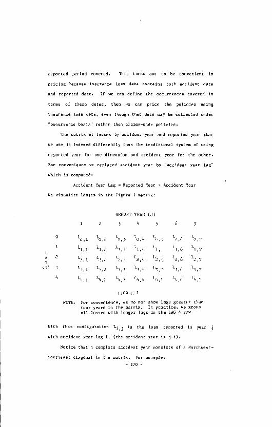
The matrix of losses by accident year and reported year that

we use Is indexed differently than the traditional system of using

reported year for one dimension and aecldent year for the other.

For convenience we replaced accident year by "accident year lag"

which is computed:

Accident Year Lag = Reported Year - Accident Year

We visualize losses in the Figure I matrix:

REPORT YEAR (J)

1 2 3 Ip 5 6 7

[. A

o ~,l Lo,2 Lo,3 tb,~ I o,5 ~1),6 to,7 1 L], 1 Li, 2 L], 3 Li, 6 Ii, [ 11, 6 L], 7

2 L2, I L?,? L2, 3 1.2 ~ 1.3, 5 L?_,6 L2, ?

=. L~, I L::. 2 L%1% L~, h T,.T g 1,~,( 1,%.2

It I,!1 , ] |911:" I , ! 1 % |.11 I I I,jj , 1'~: f. l h ,'.'

NOTE:

j.'IGIII.E i

For convenience, we do not show lags greater than four years in the matrix. In practice, we group all losses with longer lags in the LAG 4 row.

With this configuration Li, j is the loss reported in year j

with accident year lag l, (the aceldent year is j-L).

Notlce that a complete accident year consists of a Northwest-

Southeast diagonal ~n the matrix. For example:

- 270 -

Ace[dent year |

(Ace. year l, report year I) + (Ace. year |, report year 2) + ...

(Report year l, lag O) + (Report year 2, lag l)

+ (Report year 3, tag 2) + ...

LO, | + Li, 2 + L2, 3 + L3, 4 + ...

We are now in a position to describe some of the coverage

concepts in terms of the matrix above (in the examples which

follow, all policies are assumed written at the "beginning of year

J for a one-year term):

"Mature" clalms-made policy. A policy which covers claims

reported during the policy period, regardless o[ accident date.

Such a policy written at the beginning of year ] will cover the

jib column of matrix L in Figure ].

First-year claims-made policy. A policy which covers only

the "lag 0" row Of the Jth column of L. An insured in his first-

year of a clalms-made insurance program would purchase this

coverage.

Second-year claims-made policy. A policy which covers the

"lag 0" and "lag I" row of the Jth column of L. An insured in his

second year of the clalms-made insurance program would purchase

this coverage.

Occurrence policy. A policy which covers claims arising from

accidents occurring during the policy period. Such a policy would

cover a Northwest-to-Southeast diagonal of matrix L. This is the

traditional form of coverage in most liability lines.

Tall polio. A policy written for an insured who leaves the

clalms-made program. It covers losses whose aecldent date lles in

the period during which the claims-made coverage was in force, and

whose reported date Is after the insured'e last claims-made pellcy

expired.

- 271 -

Retroactive date. The earliest accident date for which

coverage is provided under a clalms-made policy. Normally this

would be the date on which an insured's first clalms-made policy

commences. Only claims with accident date subsequent to the

retroactive date are covered by any subsequent clalms-made or tall

policy.

We will illustrate these coverages with the example of a

• hypothetical insured who begins practice at the start of year 1

and retires four years later. He buys an occurrence policy to

cover his first year of practice, then switches to the clalms-made

program. He purchases flrst-year, second-year, and thlrd-year

clalms-made policies for years 2, 3, 4 respectively. At the end

of year 4, he retires and purchases a tall policy. The policies

cover the Figure I loss matrix in the manner shown in Figure 2.

REPORT YEAR

1 2 3 4 5 6

C ~ C - ~ , ~ ICLAU

FIGURE 2

7

0 L

"a 'T"

- 272 -

An important point to note is that the coverage above is

equivalent to the coverage provided under & occurrence pollcles,

as shown in Figure 3 below:

REPO!~T YEAR

i 2 5 ~ 5 C 7

\

3 ¥ Y'

FJGUI%E 3

A l t h o u g h t he c o v e r a g e to t h e i n s u r e d i s t he same unde r the

clalms-made system as under the traditional occurrence system,

there is an important difference in the timing of the premium

determination. To illustrate, the losses for report year 4 lag 2

are covered by the occurrence policy written at (and priced no

later than) the beginning of year 2. For our claims-made insured,

these losses would be covered by the thlrd-year clalms-made policy

written at the beginning of year 4. The clalms-made system

allowed the insurer an extra two years to price this "lag 2" loss

element.

- 273 -

IV. Claims-Made Ratemskin~ Principles

AS noted previously, the major differences between the claims-

made and the occurrence policy lies not in th e coverage provided, but

in the timing of pricing decisions affecting that coverage. Under

claims-made we are always pricing next year's claims. Under occur-

rence pricing we must take into account claims to be reported many

years in the future. The accuracy of any forecast is a direct

function of how far beyond the data the projection is to be carried.

A series of simple examples will illustrate this principle as it

applies to claims-made and occurrence policies.

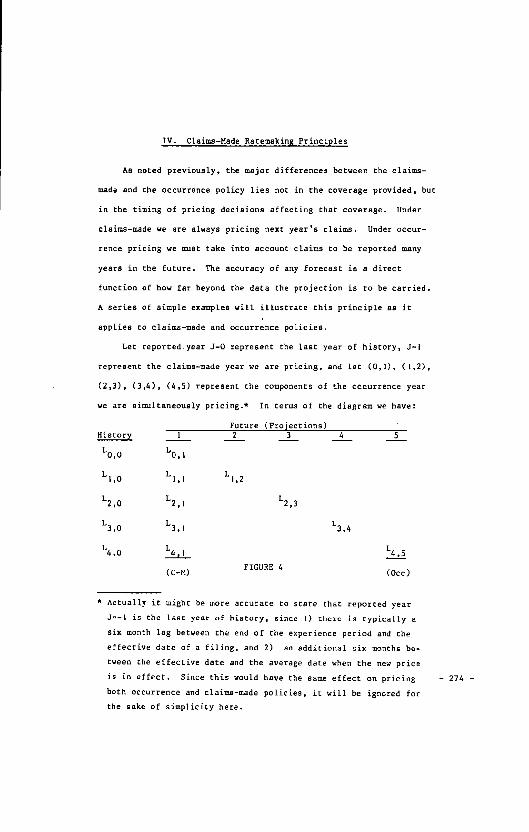
Let reported.year J=O represent the last year of history, J=]

represent the claims-made year we are pricing, and let (0,I), (1,2),

(2,3), (3,4), (4,5) represent the components of the occurrence year

we are simultaneously pricing.* In terms of the diagram we have:

Future (Projections) History I 2 3 4

LO,0 L0,1

L|,0 LI,I LI,2

L2,0 L2,i L2,3

L3,0 L3,1 L3, 4

L4,0 L4rl

FIGURE 4 (c-M)

L4,5

(Occ)

* Actually it might be more accurate to state that reported year

JE-I is the last year of history, since I) there is typically a

six month lag between the end of the experience period and the

effective date of a filing, and 2) an additional six months be-

tween the effective date and the average date when the new price

is in effect. Since this would have the same effect on pricing

both occurrence and claims-made policies, it will be ignored for

the sake of simplicity here.

- 274 -

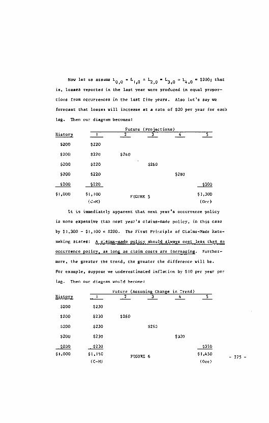
Now let us assume LO, O - Li, 0 = L2, 0 = L3, 0 = L4, O = $200; that

is, losses reported in the last year were produced in equal propor-

tions from occurrences in the last five years. Also let's say we

forecast that losses will increase at a rate of $20 per year for each

lag. Then our diagram becomes:

Future (Projections) 5 History I .2 3 4

$200 $220

$200 $220

$200 $220

$200 $220

$200 ~22o

$],000 $I,100

(C-M)

$240

$260

$280

FIGURE 5

~)oo

$],300

(Oce)

It is immediately apparent that next year's occurrence policy

is more expensive than next year's claims-made policy, in this case

by $1,300 - $I,lO0 = $200. The First Principle of Claims-Made Rate-

making states: A claims-made policy should always cost less than an

occurrence poliey~ as lone as claim costs are increasing. Further-

more, the greater the trend, the greater the difference will be.

For example, suppose we underestimated inflation by $I0 per year per

lag. Then our diagram would become:

Future (Assuming Chan~e in Trend) 2 3 4 5

$260

$290

FIGURE 6

$320

$350

$1,450

(Occ)

History I

$200 $230

$200 $230

$200 $230

$200 $230

920o $230

$ I , 0 0 0 $ I , 1 5 0

(C-M) - 275 -

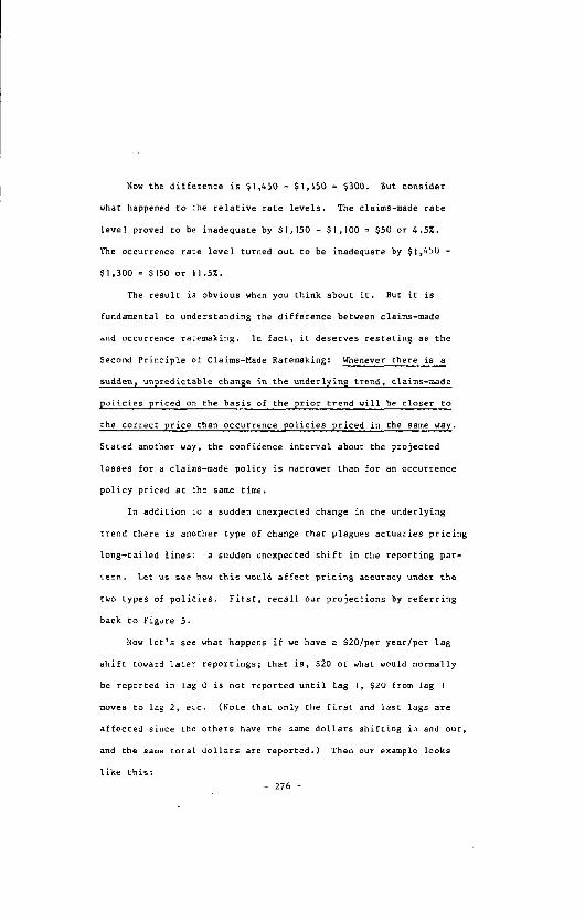
Now the difference is $1,450 - $1,150 = $300. But consider

what happened to the relative rate levels. The claims-made rate

level proved to be inadequate by $lj150 - $I,]00 = $50 or 4.5%.

The occurrence rate level turned out to be inadequate by $I,450 -

$1,300 = $150 or 11.5%.

The result is obvious when you think about it. But it is

fundamental to understanding the difference between claims-made

and occurrence ratemaking. In fact, it deserves restating as the

Second Principle of Claims-Made Ratemaking: Whenever there is a

sudden/ unpredictable chan~e in the underl~in~ trend, claims-made

policies priced on the basis of the prior trend will be closer to

the correct price than occurrence policies priced in the same way.

Stated another way, the confidence interval about the projected

losses for a claims-made policy is narrower than for an occurrence

policy priced at the same time.

In addition to a sudden unexpected change in the underlying

trend there is another type of change that plagues actuaries pricing

long-tailed lines: a sudden unexpected shift in the reporting pat-

tern. Let us see how this would affect pricing accuracy under the

two types of policies. First, recall our projections by referring

back to Figure 5.

Now let's see what happens if we have a $20/per year/per lag

shift toward later reportings; that is, $20 of what would normally

he reported in lag 0 is not reported until lag l, $20 from lag l

moves to lag 2, etc. (Note that only the first and last lags are

affected since the others have the same dollars shifting in and out,

and the same total dollars are reported.) Then our example looks

like this:

- 276 -

Future (Assumin~ Change in Repot.tins Pattern) History I 2 3 .

$200 $200 $200 $200 $200

$200 $220 $240

$200 $220 $260

$200 $220 $280

~200 $240 $280 $320 9360

$1,000 $I,I00 FIGURE 7

5

$200

$4OO

$I,380

Under these circumstances, the mature claims-made policy is

still priced correctly (as we would expect since the total dollars

reported is unchanged), although a first year claims-made policy

would have been slightly over-priced. But the occurrence policy is

under-priced by $1,380 - $1,300 = $80, or 6.2%. The Third Principle

of Claims-Made Ratemaking states: Whenever there is a sudden unex-

pected shift in the reportin~ pattern t the cost of mature claims-

made coverage will be affected very little i£ at all relative to

occurrence coverage.

If we put the two types of errors together, the result is even

more dramatic.

History

$200

$20O

$200

$200

$200

$],000

Future (Assuming Change in Trend & Shift in Reportin~ Pattern)

I 2 3 4 5

$210 $220 $230 $240 $250

$230 $260

$230 $290

$230 $320

~25o $400

$i,15o $~,s3o FIGURE 8

- 277 -

The claims-made policy is under-priced by $50 or 4.5% as be-

fore. But the occurrence policy is under-priced by $1,530 - $1,300

= $230 or 17.7%. By now, it should be obvious that claims-made

rates are both mere accurate (because of a shorter forecast period)

and more responsive to changing conditions (because external changes

affect losses as they are reported). Two other points deserve em-

phasis. Firatj claims-made policies incur no liability for IBNR

claims so the risk of reserve inadequacy is ~reatly reduced. (Prin-

ciple Number Four). For example, a company writing occurrence pol-

icies for five years at the end of the period marked "history" in

Figure 5 would carry an IBNR reserve of 4 x $220 + 3 x $240 + 2 x

$260 + I x $280 = $2,400. A company writing claims-made for the

same period would have an IBNR reserve of $0. The occurrence IBNR

reserve needed under varying assumptions would be $2,600 (Figures

6 and 7) or $2,800 (Figure 8), so either of the two unfavorable

developments would result in an IBNR reserve inadequacy of 8.33%

for the occurrence policy. The IBNR needed for the claims-made

policy is always O.

The final point follows directly from the above. Because there

is no need for IBNR, the time lapse between the collection of prem-

iums and the payment of claims is greatly reduced. Consequently, the

investment income earned from claims-made policies is substantially

less than under occurrence policies. (Principle Number 5). The longer

the reporting lag, or the shorter the settlement lag, the greater the

difference will be.* The point is, as we reduce risk of inadequate

* Algebraically, the reduction may be expressed as R/(R+$+I/2), where R

is the mean reporting lag in years, S is the mean settlement leg and

I/2 represents the I/2 year lag between payment of premium and the

occurrence of a claim on average. Of course integrals rather than

averages should really be used, but this approach produces a reason-

ably accurate answer given the uncertainties about R and S.

- 278 -

rates and insufficient reserves by switching to claims-made coverage,

we pay for it with reduced investment income. On the ether hand, the

reduced risk should allow us to write more policies for a given

amount of capacity, thus making up for the reduction in expected

profitability per policy.

Summarizing the five Principles of Claims-Made Ratemaking dis-

cussed in this section:

I) A claims-made policy should always cost less than an oc-

currence policy, as long as claim costs are increasing.

2) Whenever there is a sudden, unpredictable change in the

underlying trend, claims-made policies priced on the basis

of the prior trend will be closer to the correct price than

occurrence policies priced in the same way.

3) Whenever there is a sudden unexpected shift in the reporting

pattern, the cost of mature claims-made coverage will be

affected very little if at all relative to occurrence cov-

erage;

4) Claims-made policies incur no liability for IBNR

claims so the risk of reserve inadequacy is greatly reduced.

5) The investment income earned from claims-made policies is

substantially less than under occurrence policies.

Now that the advantages of the claims-made approach are apparent,

we will discuss how pure premium data for claims-made pricing is com-

piled, even where claims-made coverage has never been written.

- 2 7 9 -

V. Historical Pure Premium Collection

As explained above, our approach to ratemaking requlres that

we compute ht~torleal pure premiums by reported period and lag.

To do this we collect the loss data and the exposure data and form

the quotient.

Collection of Losses. It is easy enough to cateBortze

losses by reported period and lag using the coded reported date

and accident date. Since we use pure premiums on an "ultimate

value N basis, development factors are applied to the most recent

loss valuations. The development factors used in our approach

have these features:

I. They are a function of report period only.

2. The development factors are applied only to the ease

reserve portion of the loss, not to the pald component.

3. The factors are determined through a "backward recurstve"

formula, described in Appendix A.

Because the factors develop reported period losses to ultimate

value, they provide for anticipated shortages or redundancies in

case reserves, but they do not provide for IBNR (Incurred But Not

Reported) losses. There is no need for IBNR losses in the claims-

made ratemaklng process, since the primary focus Is on losses by

reported period.

Collection of Exposure. Determining the number of exposures

for each reported period and lag in more difficult than tabulating

the losses. Thls is especlally the case when the data base consists

of a mlxture of occurrence and claims-made polleles. The best way

to see the diffleulty in to look at hypothetical premlum trans-

actions and see how much each trsnsactlon contributes "earned

- 2 8 0 -

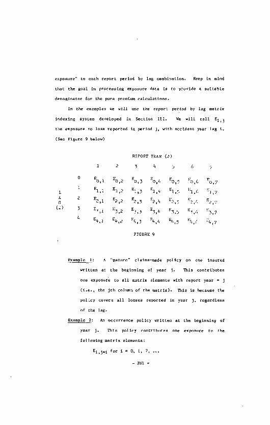
exposure" to each report period by lag combination. Keep in mind

that the goal in processing exposure data is to provide a suitable

denominator for the pure premium calculations.

In the examples we will ose the report period by lag matrix

indexing system developed in Section III. We will call El, j

the exposure to loss reported in period J, with accident year lag i.

(See Figure 9 below)

L A G

(1)

REPORT YEAR (J)

] 2 5 4 5 6 7

o Eo, I Eo, 2 EO,3 EO,4 EO,; EO,6 EO,7

i Ei,i Ei,2 El,. 5 El,4 Ei,5 E l , ( ' El,7

2 5,1 5,2 5,3 5,4 5.~ %/. ~'2,7

3 E~, 1 E3, 2 E3, 3 ES, 4 E3, 5 E~,(, E3, 7

4 E4, I E#, 2 E%, 3 E%,& E4, 5 El{,6 E4,7

FIGURE 9

Example 1: A "ma tu re " c la ims-made p o l i c y on one Insu red

written at the beginning of year J. This contributes

one exposure to all matrix elements with report year = J

(i.e., the ]th column of the matrix). This is because the

policy covers all losses reported in year J, regardless

of the lag.

Example 2: An occurrence policy written at the beginning of

year J. This policy contributes one exposure to the

following matrix elements:

El,j+ i for i = O, l, 2, ...

- 281 -

Example 3: A mature clalms-made policy written I/3 of the

way through year J. This policy contributes:

2/3 exposure to El, j for i = 0, I, 2, ...

I/3 exposure to El,j+ 1 for i - O, I, 2, ...

This is the familiar "uniform earning" which also

characterizes occurrence policies and most other

policies in property and casualty insurance.

Example 4: A second-year clalms-made policy written at the

beginning of year J. This policy generates one exposure

for only lag 0 and I portions of reported year J, (i.e.,

EO, j and El,j).

Example 5: A flrst-year clalms-made policy written I/3 of

the way (i.e., Hay I) through year ]. Before jumping to

any conclusions about the amount of exposure look at

Figure I0 on the next page. In Figure ]0,

we introduce the term "difference" as the difference

between reported date and accident date. (This is in

contrast to "lag', which is the difference between

reported year and accident year.)

In Figure IO, the solid lines delineate regions

represented by re port year-lag combinations. These

are parallelograms except for the "lag 0" region,

which is a right triangle. The shaded area is the

triangular region covered by the policy of Example 5.

We can see that the policy covers the following

- ' 282 -

D I F F E R E N IYR. C E

2. YR,

P.E P O R T DATE"

0 MAY1

, \ L A & |

' lEA R

LAG ~_

F I G U R E I 0

THIS FIGURE ILLUSTRATES THE COVERAGE OF A FIRST-YEAR CLAIMS-MADE POLICY WRITTEN ON MAY 1 OF YEAR i.

SHADED AREA REPRESENTS THE CCVERAGE OF THIS POLICY.

SOLID LINES REPRESENT BOUNDARIES OF "REPORTED YEAR -LAG" CELLS.

"DIFFERENCE" (VERTICAL AXIS) REPRESENTS THE TIME DIFFERENCE BETWEEN DATE OF ACCIDENT AND DATE OF REPORTING.

"LAG" IS REPORTED YEAR [iINUS ACCIDENT YEAR.

- 2 8 3 -

propor t ion of these regions:

2/3 x 2/3 - 4/9 of report year l, lag O;

|/3 x I/3 - I/9 of report year 2, lag 0;

I/3 x 2/3 = 2/9 of report year 2, lag I.

These proportions are the earned exposure contri-

butions to E0,1, E0,2, and El, 2 respectively.

We can see, from Example 5, that the determination of exposure

by report year and lag can be a fairly complex problem. This is

especially so for "non-mature" clalms-made policies and tall

policies. However, the graphical technique used in Figure ]0 Is

general and can be applied to any type of policy.

Before going on to a discussion of pure premium projection

we will make come observations about the earned exposure

calculations. We have concentrated on the general theory of how

to make the exposure calculation, given the "maturity" of a

clalms-m~de policy trensactlon and the actual commencement date.

In reality one may have to make these calculations using only

summarized written premiums and earned premiums by type o[ policy

and by time period (rather than using detailed transection data).

If this is this case~ accuracy is greatly improved if the time

periods are as fine as possible. Another problem which arises is

the actual determination of the "ma~urlty" of a clalms-made

policy. This requires the coding of the date on whlch an insured

first purchases clalms-made coverage (the "retroactive date").

This date is crucial and must he accurately recorded.

A simplification was made in the exposure calculation

argument based on Figure 10. Using the proportional areas of the

- 284 -

figure was equivalent to assuming a "uniform claim potential"

within each year-lag parallelogram or triangle ~n the figure.

Summary. In this section we have attempted to describe the

process by which historical pure premiums (quotient of loss and

exposure) by reported period and lag can be computed. The

tabulation of loss is straightforward, since insurance loss data

contains reported dare and accident date. The tabulation of

exposure is much more complex, since different clalms-made end

occurrence policies contribute to different report period-lag

exposure "cells".

Once these historical pure premlums are computed, the actuary

can begin the projection of future pure premiums.

- 285 -

VI. Future Pure Premium Projection

Once historic pure premiums have been calculated, future pure

premium projection proceeds in two steps. First, the future "mature"

claims-made pure premium is determined. Second, the total pure pre-

mium is distributed back to lags and hence to policies at different

levels of maturity. We will discuss each of these steps in turn.

In its simplest form, mature pure premium projection consists

of nothing more than polynomial or exponential regression, using time

as the independent variable.* This is suitable for countrywide data

and perhaps for a few high volume states. It is not suitable for most

states, however, as random fluctuation and the distortion of changes

in legal o~ social climate can produce very poor fits and unreliable

estimates. The actuary must be careful to check for this every time

he does his analysis, even for the largest states, since a sudden

surge or drop in claims being reported can occur in a single state

at any time, destroying a previously stable trend. Normally, these

events average out when countrywide data is used, although the evi-

dence of recent years indicates that the experience in all states is

becoming more highly correlated with one another.

If the actuary decides a particular state's trend is not suf-

ficiently stable or reliable to use for projecting its future mature

pure premiums, he may project them through a two-stage process. First,

* Other curves, such as log or power functions, have been proposed

as alternatives. Unfortunately, the results derived from fitting

these functions are highly dependent on the time index chosen,

since the regression is done against the log of the index rather

than the index itself.

- 286 -

the actuary generates countr~ide ,fitted ~ure premium using poly-

nomial regression as described above. Second, he applies linear

regression or "regression through the origin", with state pure

premium as the dependent variable and countrywide fitted pure pr 9-

mium as the independent variable. This approach assumes that, in

the long run, a consistent relationship exists between state and

countrywide pure premium. In other words~ it assumes that the

state will have the same percentage change from one year to the

next that all states do, while using the individual state's own

experience to determine its "relativity" to the countrywide rate.

Linear regression is similar, but adds a constant term which allows

partial recognition of the state's own apparent trend. Of course,

if linear regression is used in both stages one and two, the result

is the same as using linear regression against time directly.

Two points merit emphasis about the above procedure. First, as

always, it is the actuary's task to strike the delicate balance be-

tween stability and responsiveness. This is done directly through

his choice of a projection method, rather than indirectly through

the choice of a credibility formula. The question to be kept con-

stantly in mind is : How reliable is this data as an indicator of

the claim process in this state? Fortunately, a wealth of information

about the quality of the regression is available to help answer that

question. Second, all projections are done on the experience itself.

No "outside" frequency or severity trend information is superimposed

on the data, thus avoiding the problem of explaining two or three

sets of data and reeoncil[ng them with one another. There is no reason

why this procedure should be limited to claims-made; its advantages

apply equally well to any type of coverage.

* See Appendix B for a technical description.

- 287 -

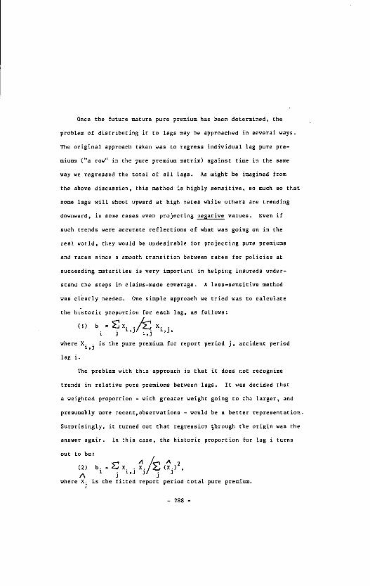
Once the future mature pure premium has been determined, the

problem of distributing it to lags may be approached in several ways.

The original approach taken was to regress individual lag pure pre-

miu~ ("a row" in the pure premium matrix) against time in the same

way we regressed the total of all lags. As might be imagined from

the above discussion, this method is highly sensitive, so much so that

some lags will shoot upward at high rates while others are trending

downward, in some cases even projecting negative values. Even if

such trends were accurate reflections of what was going on in the

real world, they would be undesirable for projecting pure premiums

and rates since a smooth transition between rates for policies at

succeeding maturities is very im~rtant in helping insureds under-

stand the steps in claiM-made coverage. A less-sensitive method

was clearly needed. One simple approach we tried was to calculate

the h~toric proportion for each lag, as follows:

(')b'~jXi'J~ijXi'j'i

where X. . is the pure premium for report period j, accident period 1,3

lag i.

The problem with this approach is that it does not recognize

trends in relative pure premiums between lags. It was decided that

a weighted proportion - with greater weight going to the larger, and

presumably more recent,observations - would be a better representation.

Surprisingly, it turned out that regression through the origin was the

answer again. In this case, the historic proportion for lag i turns

out to be:

~/~j ~ )2 (2) b i =EEl, j . Xj (Xj ,

l where X. is the fitted report period total pure premium.

]

- 288 -

Let's see how this compares to the historic proportion cal-

culated above. Note that:

~i~xij and~ °~x ~ x .... Xj • , j I j J ° i , j ~ ' J

Therefore, (I) can be re-written as follows:

b i

b i ~ X..~.~X j z'31 j i

Thus, we see the difference between (]) and (2) is simply that

A the Xj, s are used as weighting factors to place greater weight on

larger pure premiums. It is important to note that ~b i = ! since i'

the bi, s are the fractions of the total pure premium associated with

each lag.

Summing up, the projection of pure premiums may be viewed as a

two-step process. First, project the total {"mature") pure premium

ignoring lags. Second, distribute the total pure premium back to lags.

Several methods for carrying out each step have been suggested in this

section.

There is no one "right" method for all circumstances. In fact,

once the data is collected into a historic pure premium matrix, the

possibilities for projection methods are limited only by the actuary's

imagination and the flexibility of his statistical software package.

For example, both econometrics and time series analysis merit explor-

ation since the pure premium data by reported year seems to indicate

distinct cycles about the long term trend line roughly corresponding

l, i

* This is true, if and only if, the Xj, s were arrived at through

linear regression. For regression through the origin, the residuals

do not sum to zero. - 289 -

to the economic cycle. This is logical since the incidence of

malpractice should vary only with the utilization of medical ser-

vices, while the reporting of a claim has a lot to do with how the

claimant feels about his own economic situation. In any case, we

suggest a "simulation" approach be used as a means of sensitivity

analysis.

At the St. Paul, we divide states into four categories:

A - States, with highly stable patterns, where we use re-

gression on their total pure premiums to determine their

own trend;

B - States, where we use regression through the origin for

both the total and lag pure premium;

C - States, where we use regression through the origin for

the total pure premium but use the countrywide lag pat-

tern and;

D - States, with very thin data, where we use a judgmental

relativity to the countrywide pure premium.

As noted earlier, the categorization of each state must be re-

viewed each year to make sure changes in claim environment have not

materially altered the data's reliability. Sensitivity analysis

provides valuable insights in this process as well.

The ability to project pure premiums allows the actuary to de-

termine more than prices for claims.made policies. Specifically, it

can also be used to price occurrence policies, and to predict IBNR

emergence and reserve adequacy. We will have more to say on this in

Section Vlll. But first, we will briefly discuss some special features

of The St. Paul filings which distinguish them from those of other

claims-made writers.

- 2 9 0 -

Vll. Special Features of St. Paul Claims-Made Filings

Not all elaims-ulade policies are alike in coverage. The St.

Paul claims-made form contained several unique (at the time) cov-

erage features which presented the actuaries with special pricing

problems. Also, we chose several pricing techniques which were not

traditional to facilitate the process of claims-made ratemaking

from occurrence data. We will briefly discuss each of these special

features in turn.

Several unique features of The St. Paul filings have already

been discussed in Section III. One of these was the retroactive

date; i.e., the earliest accident dete for which coverage is pro-

vided under the claims-made policy. Previous claims-made or "dis-

covery" policies treated all insureds the same, even if they bad

no prior exposure (e.g., just coming out of medical school) or if

they were previously covered by an occurrence policy.

Another concept mentioned earlier was "tail coverage". When we

introduced claims-made we felt it was the wave of the future. Some-

day all insureds would be using it and insureds would move from one

carrier to another, carrying their retroactive dates with them.

However, we recognized that this might not occur for many years and

decided that we would have to offer our claims-made insureds guaranteed

coverage for the "tail"; i.e., for claims which occurred while the

insured was covered by claims-made but were not reported until after

the last claims-made policy had expired. This was considered a rather

dangerous step, since it in effect gave the insured the right to con-

vert his coverage from claims-made to occurrence at any time. Were

we leaving ourselves open to the same pricing problems we had had

under occurrence7 We argued t h a t the r i s k could be g r e a t l y reduced

- 2 9 1 -

by selling the tail coverage in three annual installments, or

reportin 8 endorsements, reserving the right to price them one

at a time. The first reporting endorsement would be just like

the insured's next claims-made policy, providing coverage for

claims reported during that year only, except that accidents occur-

ring in that year would be excluded. The second reporting endorse-

ment would be similar, except that accidents occurring in the two

year period after expiration of the last claims-made policy would

not be covered. Only the third reporting endorsement would pro-

vide the kind of perpetual coverage that the occurrence policy did,

with similar pricing hazards. It was argued that that hazard was

acceptable since I) we would be pricing it at least three years

later than we would have priced the comparable coverage under an

occurrence policy; 2) each insured would buy this "occurrence"

coverage only once instead of every year, while the great majority

of insureds were ~till buying claims-made; and 3) by the time we

reach the third reporting endorsements the proportion of claims re-

maining to be reported is fairly small, so even a large percentage

error in the rate would not result in a large dollar loss.

As we discussed the claims-made concept with our insureds, it

became apparent that the three-pay reporting endorsement concept was

acceptable to the majority but could work a real hardship for a few.

So we added an additional option: We would sell a sin$1e-payment re-

portin s endorsement to any insured terminating coverage due to death,

disability or retirement.

The pricing of reporting endorsements - both three-pay and single-

pay - poses no special problems. It merely requires trending the pro-

jected pure premiums further into the future. In fact, since the

- 292 -

policy is essentially selling IBNR coverage, the pricing of re-

porting endorsements is equivalent to the determination of IBNR

reserves, which will be discussed in Section VIII. Before pro-

ceeding to that discussion, however, we will briefly mention three

special features of The St. Paul rate filings not directly linked

to the coverage provided.

The St. Paul's claims-made policy is on an annual basis. But

semi-annual reporting periods and lags were used in calculating and

projecting pure premiums. The advantages of using this approach are

twofold:

i. Less distortion calculating the earned exposures by "cell"

(See Section IV), and

2. More data points for use in the regression.

Underlying the whole idea of pricing claime-mede coverage from

occurrence data is the implied assumption that the same body of claims

would be reported at the same time under either policy. The more we

thought about it, the less reasonable this assumption see~ed. We de-

cided that two changes were likely to occur at the transition point,

both due to insureds understanding that coverage for a particular

claim would not commence until the claim had been reported.

First, we assumed that, on average, claims would be reportsd

sooner. Specifically, we assumed a two-month "shift" forward in claim

reporting; algebraically,

L ~ = L0, + |/6 L I O,i I , 2

L i , 2 = L i , 2 I / 6 L i , 2 + I / 6 L2 , 3 e t c .

Second, we assumed that there would be some additional reporting

of incidents that would never have come in under the occurrence policy.

Few, if any, of these incidents would result in loss payment, but they

- 293 -

would require investigation and hence loss expense payment.

Specifically, we assumed 5% additional claim dollars would be

reported, and that all of this additional activity would come

in at Lag O. Algebraically,

L~, I = LO, I + ,05 x L i , 1

We can never know what would have been reported had we con-

tinued with the occurrence policy, so it is impossible to test

whether or not the "shift" and the additional incident reporting

actually occurred. Now that several years of claims-made ex-

perience is contained in the data base, the need for this special

adjustment no longer exists and it has been dropped from the filing.

The final special feature of the St. Paul filings involves the

treatment of company expense. It was obvious that the pure premium

and hence the rate for a first-year claims-made policy would be much

less than for a mature policy. It did not follow that all expenses

would be proportionately lower. In fact, most company expenses are

probably fixed: i.e., they do not vary with the size of the premium.

This was recognized by splitting the expense dollar into two parts:

fixed and variable. This affected not only the relativities between

different policy maturities, but between different classes of risk

as well: the higher the rate, the lower the expense ratio. Alge-

braically, the rate calculation changed from:

R - PP/(I-E-P)

to R ~ (PP + FE)/(I-VE-P)

where R is the rate, PP is the pure premium, P is the profit allow-

ance and E = FE + VE is the expense, broken down into its fixed and

variable components. The following example will illustrate how

this early instance of "expense flattening" works.

- 294 -

Fure Fixed Variable Expenses Premium Expenses and Pro.fit

(Relativity) (% of Race) (25% o f Rate) (Relativit..y..~.

Class I Physician, First-Year Claims-Made Policy

$ioo $35 (1.00) (19.4%)

$45 $180 (].oo)

Class I Physician, Mature Claims-Made Policy

$500 $35 (5.00) (4.9%)

$ i78 $713 (3.96)

Class 7 Surgeon, First-Year Claims-Made Policy

$8oo $35 (8.oo) (3.1%)

$278 $I,113 (6.19)

Class 7 Surgeon, Mature Claims-Made Policy

$4,000 $35 (40.00) (0.56%)

$1,345 $5,380 (29.89)

FIGURE l I

- 295 -

Vlll. Other Uses of Analytical Tools Developed

The techniques dlscussed in this article were developed

specifically to price the clalms-made coverages. However, once we

develop a method to project pure premiums by future report year

and lag, we have developed a tool which we can use to solve a

variety of insurance problems. We can price occurrence coverages

by adding up the appropriate elements from Figure I of Section Ill.

For example, the projected pure premium for an occurrence policy

eo~encing at the beginning of year 3 is straightforward:

XO, 3 + Xi, 4 + X2, 5 + X3, 6 + ...,

where Xi, j is the projected pure premium for reported year

J, lag i.

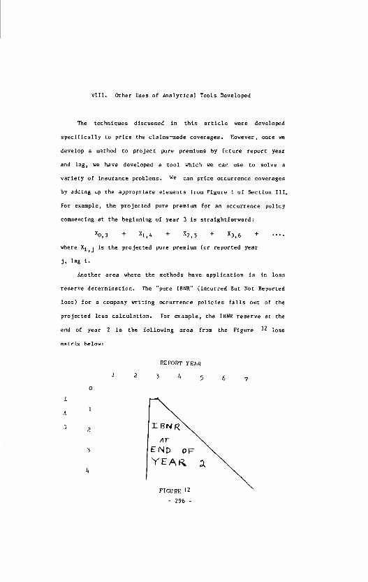
Another area where the methods have application is in loss

reserve determination. The "pure IBNR" (Incurred But Not Reported

loss) for a company wrftlng occurrence policies falls out of the

projected loss calculation. For example, the IBNR reserve st the

end of year 2 is the following area from the Figure ]2 loss

matrix below:

0

1

4

1 2

REFORT YE,~R

} 4 5 6 7

- 296 -

That fs~ the IBNR as of the end o[ year 2 on occurrence poltcles

is the sum of all losses wlth reported year greater than 2 and

accident year less than 3.

Determining "pure IBNR" is only half the problem of

determining a total loss reserve. Ore must also project the

additional development to be incurred on case reserves (reserves

on losses already reported). Thls latter problem must be solved

before we even begin to project the pure premlums In Section VI.

It turns out that the case reserve development is easier to

project once the loss data Is collected Into the report year by

lag format of Figure 1. Appendix A discusses the precise method

by which we project this case development.

Thus, the method of analyzing data which was developed to

price clalms-made policy gives us a convenient way of separating

loss development into Its two major components and projecting each

separately:

Antic ipated loss development - IBNR + Case Development.

Moreover, the method also projects an e~ergenee pattern for the

IBNR Loss.

- 2 9 7 -

IX. Summary

We began this paper by discussing the historical situation

which led to the declalon to write medical malpractice on a

clalms-made basis (Section II). Next we translated the problem of

pricing the claims-made coverages Into the problem of determining

pure premiums by report period and accident period "lag" (Section

lll). Section IV presented a discussion of clalms-made ratemaking

principles.

Next followed a technical discussion of how to calculate

historical pure premiums by report period and lag given insurance

loss and exposure data (Section V). Once this Is accomplished

there are a variety of techniques available to project future

pure premlt~as, and hence rates (Section VI). The St. Paul

claims-made program and pricing techniques have several unique

features (Section VII). Finally, the analytical tools used in

clalms-made ratemaking can also be applied to the general problem

of IBNR determination for occurrence policies (Section VIII).

- 2 9 8 -

Appendix A

The Backward Recursive Reserve Development Method

In claims-made ratemaklng the losses for each reported period

must be developed to their ultimate value. We used a "Backward

Recursive" reserve development method to accomplish this.

This method requires that loss data be available by reported

period and "age". (Age 0 means the valuation as of the end of the

reported period, age I is the valuation one period later, etc.)

It also requlres that the losses be separated into paid and case

reserve components.

The "Backward Rec ursive" method calculates development

factors which are applied to the reserve component of less only.

The determination of these factors proceeds in two steps:

|. "One-step" factors are calculated to develop losses as of

each age to the next age. Two factors are calculated for

each age k. Pk is the proportion of reserves of age k

which ~rlll be pald by age k+l. R k is the ratio of

reserves at age k+l to reserve at age k.

2. Ultimate factors are generatedlfrom the "one-step"

factors. These factors apply to the reserves at age

k to bring them to ultimate valuation.

The calculation of the none-step" factors Is a straight-

forward tabulation of the data. The factors are simply the

following:

Pk TM (Paid as of age k+l - Paid as of age k)/(Aga k reserve)

R k = (Reserve as of age k+l)/(Reserve as of age k).

In order to generate the development factors to take reserves

to their ultimate valuation, we need to assume an "ultimate" age,

t h a t i . . . . . g e N a f t e r w h i c h - - ~ - n ° 2 f ~ r t h e r d e v e l o p m e n t . . . . . . The

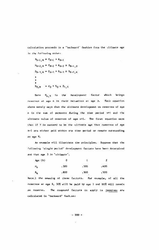
calculation proceeds i n a "backward" fashion from the ultimate age

in the following order:

DN-I,N = PN-I + RN-|

DN-2,N = PN-2 ~ RN-2 x DN_|, N

" PN-3 + RN-3 x DN_2, N DN-3,N

DO, N = PO + RO x D i , H

Here Dn, N is the development factor which brings

reserves at age n to their valuation at age N. Each equation

above merely says that the ultimate development on reserves of age

n is the sum of payments during the time period n+] and the

ultimate value of reserves of age n+l. The first equation says

that if N is assumed to be the ultimate age then reserves of age

N-I are el=her paid within one time period or remain outstanding

at age N.

An example will illustrate the principles. Suppose that the

following "single period" development factors have been determined

and that age 3 is "ultimate".

Age (k) 0 1 2

Pk .300 .500 .400

R k .800 • 500 .500

Recall the meaning of these factors. For example, of all the

reserves at age 0, 30% wlll he paid by age 1 and 80% will remain

as reserve. The compound factors to apply to reserves are

calculated in "backward" fashion:

- 3 0 0 -

D2, 3 = ,400 + .S00 - .900

D i , 3 - .500 + .500 x ( . 9 0 0 ) - .950

D0, 3 - .300 + .800 x ( . 9 5 0 ) ~ 1.060

- 3 0 1 -

Appendix B

Regression Through the Origin

"Regression through the Origin" Is s least-squares

statistical technique similar to linear regression, except that

the llne of best fit is constrained to pass through the "Origin'.

Like linear regression this technique uses a llne of "best fit" t o

fit a set of observations of some dependent variable to a set of

observations of an independent variable. Unlike linear

regression the llne of best fit is constrained so that~ when the

value of the independent variable is zero, the fitted value of the

dependent variable is also zero. The criterion for "best fit" is

the same for both techniques: the Ifne of best fit is chosen to

minimize the sum of the squares of the differences between the

observed and fitted values of the dependent variable.

There are two situations where Regression through the Origin

might be substituted for linear regression. The first is the case

where, a priori, the value of the dependent variable must be zero

when the independent variable is zero. The second situation is

one where linear regression has been run, hut the "intercept" is

not significantly different from zero, so that it can be dropped

without hurting the accuracy of the model.

An example of a problem where Regression through the Origin

might "be used is the" problem of projecting one company's output as

a function of an industry's total output, given historical annual

figures. If the second variable takes on a value of zero, the

first must also.

The structure and mechanics of Regression through the Origin

are similar to linear regression. The modeler has a~ hand

- 302 -

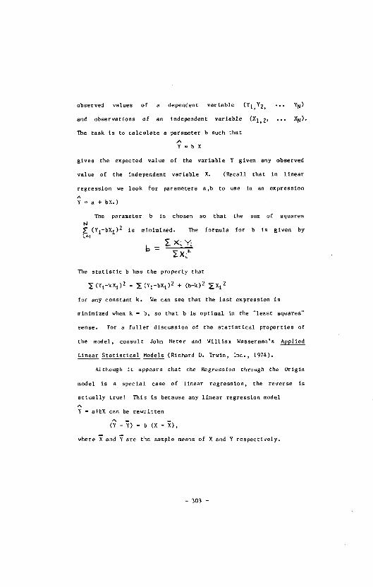
observed values of a dependent variable (Yi,Y2, ... YN )

and observations of an Independent variable (Xi, 2, ... XN).

The task Is to calculate a parameter b such that

~=bX

g i v e s the expec ted v a l u e of the v a r i a b l e Y g i v e n any obse rved

v a l u e o f the i ndependen t v a r i a b l e X. ( R e c a l l t ha t in i t n e a r

r e g r e s s i o n we look fo r pa ramete r s a , b to use In an e x p r e s s i o n

~ = a + b X . )

The parameter b Is chosen so that the sum of squares

(Yi-bXI) 2 is minimized. The formula for b is g i v e n b y

~. x~ y:

- ~_ X : ~

The statistic b has the property that

(YI-kX~) 2 = X (YI-BXi) 2 + (b-k) 2 ~Xi 2

for any constant k. We can see that the last expression is

minimized when k ~ b, so that b is optimal In the "least squares"

sense. For a fuller discussion of the statistical propertles of

the model, consult John Neter and William Wassermsn's Applied

Linear Statistical Models (Richard D. Irwin, Inc., 1974).

A/though it appears that the Regression through the Origin

model Is a special case of linear regression, the reverse Is

actuslly true! Thls Is because any linear regression model

Y - a+bX can be rewritten

(3 ~-b(X-:>, where ~ and ~ are the sample means of X and Y respectively.

- 303 -

With this formulation we can see that any linear regression model

is a speclal case of Regresslon through the Origin in which each

variable has zero mean.

- 304 -