Embed Size (px)
Citation preview
Ras-Raf MM-PB(GB)SA Tutorial: AMBER 7
Bethany L. Kormos and David L. Beveridge*
Department of Chemistry and Molecular Biophysics Program, Wesleyan University, Middletown, CT 06459
Introduction
The examples in this MM-PB(GB)SA tutorial are distributed with AMBER 71,2 and may
be found in the following directory:
~/amber7/src/mm_pbsa/Examples
This tutorial is based on calculations performed with Amber 71,2 and DelPhi II3 on an SGI Origin
200 running Irix 6.5.5. The tutorial content is basically the same for the different versions of
Amber, however there are differences in implementation and technical details between the
versions, thus they have been divided into separate tutorials.
Contained within the ~/amber7/src/mm_pbsa/Examples directory are six examples for
how the MM-PBSA program may typically be used in AMBER. One of the capabilities offered
within the MM-PBSA module in AMBER that is not covered in these examples is the alanine
scanning technique.4 These examples have been drawn from studies performed by Case and
coworkers5,6 on a protein-protein complex (H-Ras/C-Raf1).
Summary of Theory
The calculations described herein as MM-PBSA or MM-GBSA may also be more
precisely designated as MD-PBSA or MD-GBSA. This genre of theoretical calculations is
additionally referred to by several different names in the recent literature, including master
equation,7 end point8 calculations, and component analysis.9-11 The overall objective of these
methods and this tutorial is to calculate the absolute binding free energy for the non-covalent
association of any two molecules, A and B, in solution, i.e.
*][][][ **aqaqaq BABA ⇔+
where [A]aq refers to the dynamical structure of molecule A free in solution, [B]aq refers to the
dynamical structure of molecule B free in solution, and [A*B*]aq* represents the complex formed
from molecules A and B, taking into account any structural changes ([A*] and [B*]) and solvent
reorganization (aq*) that may occur upon complex formation.
In principle, this calculation requires three MD simulations, one each on [A]aq, [B]aq, and
[A*B*]aq*. Gohlke and Case6 refer to this protocol as “separate trajectories” or “three
trajectories” (3T). However, in this tutorial, one makes the (questionable) approximation that
structural adaptation is negligible and draws the trajectories for [A]aq and [B]aq from the single
MD carried out on [A*B*]aq*, simply by separating the complex into its constituent parts, [A*] aq*
and [B*] aq* (1T). The extension to the 3T protocol should be straightforward starting from this
tutorial.
The following is a summary of the thermodynamic quantities determined in this tutorial.
The binding free energy for the noncovalent association of two molecules may be written as:
( ) BAAB GGGABBAG −−=→+∆
The free energy of any molecule X may be divided into a contribution from the solute and a
contribution from the solvent:
( ) ( ) ( )XGXGXG solventsolute +=
The free energy contribution from the solute may be expressed as:
( ) ( ) )(XTSXUXG solute −=
where:
( ) )(XEXU =
( ) configvibrottrans SSSSXS +++=
Here, ⟨E(X)⟩ represents an average of energies obtained from the MD simulation(s),
Strans and Srot are the entropic contributions from translational and rotational motion, respectively,
obtained from classical statistical mechanics,
Svib is the entropic contribution from vibrational motion, obtained from a normal mode
calculation in this tutorial, and
Sconfig is the configurational entropy contribution from sidechain reorganization. Note that
configurational entropy is neglected in this protocol, but may be significant.
2
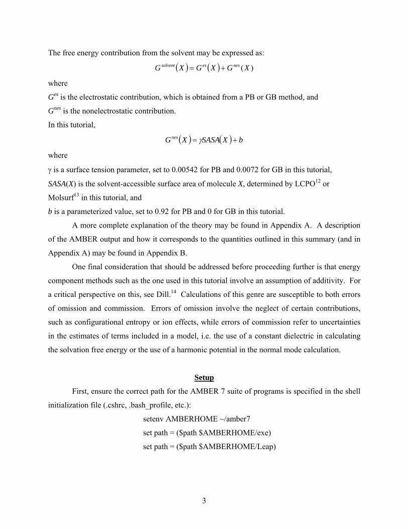
The free energy contribution from the solvent may be expressed as:
( ) ( ) )(XGXGXG nesessolvent +=
where
Ges is the electrostatic contribution, which is obtained from a PB or GB method, and
Gnes is the nonelectrostatic contribution.
In this tutorial,
( ) ( ) bXSASAXGnes += γ
where
γ is a surface tension parameter, set to 0.00542 for PB and 0.0072 for GB in this tutorial,
SASA(X) is the solvent-accessible surface area of molecule X, determined by LCPO12 or
Molsurf13 in this tutorial, and
b is a parameterized value, set to 0.92 for PB and 0 for GB in this tutorial.
A more complete explanation of the theory may be found in Appendix A. A description
of the AMBER output and how it corresponds to the quantities outlined in this summary (and in
Appendix A) may be found in Appendix B.
One final consideration that should be addressed before proceeding further is that energy
component methods such as the one used in this tutorial involve an assumption of additivity. For
a critical perspective on this, see Dill.14 Calculations of this genre are susceptible to both errors
of omission and commission. Errors of omission involve the neglect of certain contributions,
such as configurational entropy or ion effects, while errors of commission refer to uncertainties
in the estimates of terms included in a model, i.e. the use of a constant dielectric in calculating
the solvation free energy or the use of a harmonic potential in the normal mode calculation.
Setup
First, ensure the correct path for the AMBER 7 suite of programs is specified in the shell
initialization file (.cshrc, .bash_profile, etc.):
setenv AMBERHOME ~/amber7
set path = ($path $AMBERHOME/exe)
set path = ($path $AMBERHOME/Leap)
3
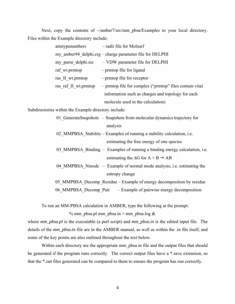
Next, copy the contents of ~/amber7/src/mm_pbsa/Examples to your local directory.
Files within the Example directory include:
atmtypenumbers – radii file for Molsurf
my_amber94_delphi.crg – charge parameter file for DELPHI
my_parse_delphi.siz – VDW parameter file for DELPHI
raf_wt.prmtop – prmtop file for ligand
ras_II_wt.prmtop – prmtop file for receptor
ras_raf_II_wt.prmtop – prmtop file for complex (“prmtop” files contain vital
information such as charges and topology for each
molecule used in the calculation)
Subdirectories within the Example directory include:
01_GenerateSnapshots – Snapshots from molecular dynamics trajectory for
analysis
02_MMPBSA_Stability – Examples of running a stability calculation, i.e.
estimating the free energy of one species
03_MMPBSA_Binding – Examples of running a binding energy calculation, i.e.
estimating the ∆G for A + B AB
04_MMPBSA_Nmode – Example of normal mode analysis, i.e. estimating the
entropy change
05_MMPBSA_Decomp_Residue – Example of energy decomposition by residue
06_MMPBSA_Decomp_Pair – Example of pairwise energy decomposition
To run an MM-PBSA calculation in AMBER, type the following at the prompt:
% mm_pbsa.pl mm_pbsa.in > mm_pbsa.log &
where mm_pbsa.pl is the executable (a perl script) and mm_pbsa.in is the edited input file. The
details of the mm_pbsa.in file are in the AMBER manual, as well as within the .in file itself, and
some of the key points are also outlined throughout the text below.
Within each directory are the appropriate mm_pbsa.in file and the output files that should
be generated if the program runs correctly. The correct output files have a *.save extension, so
that the *.out files generated can be compared to them to ensure the program has run correctly.
4
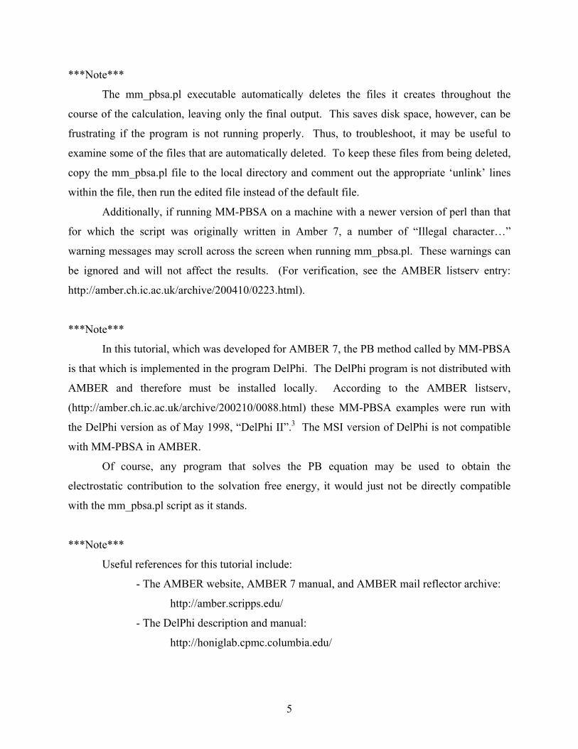
***Note***
The mm_pbsa.pl executable automatically deletes the files it creates throughout the
course of the calculation, leaving only the final output. This saves disk space, however, can be
frustrating if the program is not running properly. Thus, to troubleshoot, it may be useful to
examine some of the files that are automatically deleted. To keep these files from being deleted,
copy the mm_pbsa.pl file to the local directory and comment out the appropriate ‘unlink’ lines
within the file, then run the edited file instead of the default file.
Additionally, if running MM-PBSA on a machine with a newer version of perl than that
for which the script was originally written in Amber 7, a number of “Illegal character…”
warning messages may scroll across the screen when running mm_pbsa.pl. These warnings can
be ignored and will not affect the results. (For verification, see the AMBER listserv entry:
http://amber.ch.ic.ac.uk/archive/200410/0223.html).
***Note***
In this tutorial, which was developed for AMBER 7, the PB method called by MM-PBSA
is that which is implemented in the program DelPhi. The DelPhi program is not distributed with
AMBER and therefore must be installed locally. According to the AMBER listserv,
(http://amber.ch.ic.ac.uk/archive/200210/0088.html) these MM-PBSA examples were run with
the DelPhi version as of May 1998, “DelPhi II”.3 The MSI version of DelPhi is not compatible
with MM-PBSA in AMBER.
Of course, any program that solves the PB equation may be used to obtain the
electrostatic contribution to the solvation free energy, it would just not be directly compatible
with the mm_pbsa.pl script as it stands.
***Note***
Useful references for this tutorial include:
- The AMBER website, AMBER 7 manual, and AMBER mail reflector archive:
http://amber.scripps.edu/
- The DelPhi description and manual:
http://honiglab.cpmc.columbia.edu/
5
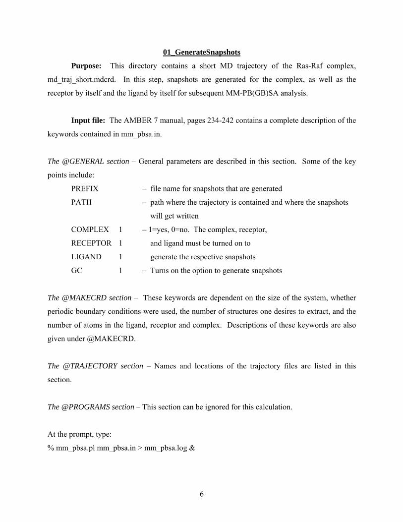
01_GenerateSnapshots
Purpose: This directory contains a short MD trajectory of the Ras-Raf complex,
md_traj_short.mdcrd. In this step, snapshots are generated for the complex, as well as the
receptor by itself and the ligand by itself for subsequent MM-PB(GB)SA analysis.
Input file: The AMBER 7 manual, pages 234-242 contains a complete description of the
keywords contained in mm_pbsa.in.
The @GENERAL section – General parameters are described in this section. Some of the key
points include:
PREFIX – file name for snapshots that are generated
PATH – path where the trajectory is contained and where the snapshots
will get written
COMPLEX 1 – 1=yes, 0=no. The complex, receptor,
RECEPTOR 1 and ligand must be turned on to
LIGAND 1 generate the respective snapshots
GC 1 – Turns on the option to generate snapshots
The @MAKECRD section – These keywords are dependent on the size of the system, whether
periodic boundary conditions were used, the number of structures one desires to extract, and the
number of atoms in the ligand, receptor and complex. Descriptions of these keywords are also
given under @MAKECRD.
The @TRAJECTORY section – Names and locations of the trajectory files are listed in this
section.
The @PROGRAMS section – This section can be ignored for this calculation.
At the prompt, type:
% mm_pbsa.pl mm_pbsa.in > mm_pbsa.log &
6
Output files: After you have executed mm_pbsa.pl you will see five snapshots of the
complex (ras_raf_II_wt_com.crd.#), receptor (ras_raf_II_wt_rec.crd.#), and ligand
(ras_raf_II_wt_lig.crd.#).
02_MMPBSA_Stability
Purpose: The mm_pbsa.in file in this directory computes continuum free energy
estimates with both PB and GB methods to verify convergence (stability) of the energies. In this
calculation, the energy components for the five snapshots of the COMPLEX that were generated
in Part 1 are computed; they could also of course be computed for the ligand and/or the receptor.
Input file:
The @GENERAL section:
The complex is turned on while the ligand and receptor are turned off.
The keywords COMPT, LIGPT, RECPT refer to the path of the prmtop files for the
various molecular species.
The keywords MM, GB, PB, MS are turned on:
MM – Calculation of gas-phase energies using Sander
GB – Calculation of solvation free energies using the GB models in Sander
PB – Calculation of solvation free energies using DelPhi
MS – Calculation of nonpolar contributions to solvation using Molsurf. If MS =
0, nonpolar contributions are instead calculated with the LCPO method in Sander.
Each of the programs used to compute the different energy contributions have different
associated parameters to be specified, thus they each have a section in the input file in which this
may be done:
The @DELPHI section – these are the keywords supplied to the DelPhi program. Keyword
descriptions have been taken from the DelPhi manual and condensed for a synopsis of the most
pertinent points:
7
INDI – the dielectric constant of the solute. The input file has it set at 1.0, which
corresponds to a molecule with no polarizability (the state assumed in most molecular mechanics
applications). INDI=2 represents a molecule with only electronic polarizability. INDI=4-6
represents a small reorganization of molecular dipoles not explicitly represented. According to
Gilson and Honig,15 materials with a similar dipole density, dipole moment and flexibility such
as globular proteins have a dielectric between 4 and 6. Any process where large conformational
changes and reorientation of dipoles occurs should not use a simple dielectric constant and
should instead be modeled explicitly.
EXDI – external dielectric (solvent); 80.0=water
PERFIL – the percentage of the lattice that the largest part of the molecule will fill.
Larger percentage fills provide a more detailed mapping of the molecular shape onto the lattice.
However, a very large fill brings the dielectric boundary of the molecule closer to the lattice
edge, which may cause larger errors arising from the boundary potential.
SCALE – reciprocal of one grid spacing (grids/angstrom)
LINIT – number of iterations with the linear PB equation. Suggested that enough
iterations be performed to give a final maximum change in potential at the grid points of less
than 0.001 kT/e. Number of iterations needed will increase with GSIZE, decrease with
decreasing PERFIL, and decrease with increasing ionic strength.
BNDCON – type of boundary condition imposed on the edge of the lattice. BNDCON=4
represents a coulombic potential.
CHARGE and SIZE – names of the charge and size files required by DelPhi. To create
these files for other systems, consult the DelPhi manual.
SURFTEN and SURFOFF – parameters used to compute the nonpolar contribution of the
solvation free energy. Values used in this input file are literature values for DelPhi.
***NOTE***
According to the AMBER listserv, the values used in DelPhi should be:
SURFTEN = 0.00542
SURFOFF = 0.92 (NOT 0.092, which is in the original input file)
(see http://amber.ch.ic.ac.uk/archive/200409/0013.html)
8
Finally, there are other keywords in the DelPhi program which may or may not be useful
in this section, i.e. SALT (salt concentration), NONIT (to use the non-linear PB equation),
PRBRAD (the radius of the probe molecule that defines the SASA), AUTOC (automatically
calculates number of iterations required for convergence), etc. However, additional keywords
cannot just be added to the mm_pbsa.in file, the mm_pbsa.pl file must also be edited to
recognize the new keywords.
The @GB section – These are the keywords supplied to Sander in AMBER to run GB:
IGB – the generalized born solvation model used. Choices are outlined in the input file
as well as in the AMBER manual. Methods differ between AMBER versions. See Appendix C
for a brief description of the GB methods available in AMBER 7.
SALTCON – sets concentration (M) of mobile counterions in solution.
EXTDIEL – solvent dielectric constant (default = 78.5 in Sander)
SURFTEN and SURFOFF – parameters used to compute the nonpolar contribution of the
solvation free energy. SURFOFF is not a keyword available in Sander, so it will always be set to
0.0 as in the input file. However, SURFTEN = 0.0072 in the input file is slightly different than
the default value in Sander (SURFTEN = 0.005). Changing the value of SURFTEN in this test
case from 0.0072 to 0.005 changes the resultant energy fairly significantly, with an overall
difference of 25.07 kcal/mol in GBTOT, a value larger than the standard deviations computed.
A value of 0.0072 is recommended for calculations in which AMBER charges are used,16 while
the value of 0.005 should be used with PARSE charges.17
Other GB keywords in Sander that may or may not be useful in this section include,
INTDIEL (interior dielectric constant, default = 1), etc.
***NOTE***
The different IGB methods require different atomic radii that are read in from the prmtop
files. This is accomplished using different “set default PBradii” commands when preparing the
prmtop files in LEaP. Consult the AMBER 7 manual and/or Appendix C of this tutorial for
further details.
9
The @MS section – These are the keywords supplied to the Molsurf program. Molsurf is used to
compute the solvent accessible surface area (SASA) of the solute,13 which is used to determine
the hydrophobic contribution to the solvation free energy:
PROBE – radius of the probe used to calculate the SASA
RADII – name of the radii file; use the atmtypenumbers file provided
The @PROGRAMS section:
Remember to specify the correct path for the DelPhi executable under the keyword
“DELPHI.”
Again, use the mm_pbsa.in input file provided and type the command:
% mm_pbsa.pl mm_pbsa.in > mm_pbsa.log &
Output files: The energy components for the five structures are listed in the file
ras_raf_II_wt_all.out.save, and the average value for each component averaged over the five
snapshots and associated standard deviations are listed in the file
ras_raf_II_wt_statistics.out.save. Notice that no entropic terms are included, so this is not a true
free energy value.
03_MMPBSA_Binding
Purpose: The mm_pbsa.in file in this directory may be used to compute the free
energies of binding for the process A + B AB, in this case the association of ras with raf to
form the complex.
Input file:
The @GENERAL section:
This time, the ligand, receptor, and complex are all turned on, and the terms MM, GB,
PB, and MS are computed for EACH species. The remainder of the input file is set up exactly
the same as it was in Part 2.
10
Remember to specify the correct path under the keyword “DELPHI” within the section
@PROGRAMS in the mm_pbsa.in file.
Use the input file provided and type:
% mm_pbsa.pl mm_pbsa.in > mm_pbsa.log &
Output files: The three output files, ras_raf_II_wt_rec.all.out.save,
ras_raf_II_wt_lig.all.out.save, and ras_raf_II_wt_com.all.out.save, contain the energy
components for each the five snapshots generated in the first part of the tutorial for the receptor,
ligand and complex, respectively. The file, ras_raf_II_wt_statistics.out.save, lists the energy
components for complex, receptor, and ligand separately, followed by the difference in energy
between the complex and the free species (under the category DELTA). Notice that no entropic
terms are included, so this is not a true free energy value.
04_MMPBSA_Nmode
Purpose: The mm_pbsa.in file in this directory turns on the NM keyword, which is used
to calculate the entropy of the ligand using the NMODE program in AMBER. The NMODE
program may additionally be used to search for transition states, perform a Newton-Raphson
minimization, or perform a langevin mode calculation. In this section, first, a conjugate-gradient
minimization is performed on each of the five structures of the ligand. Then, the nmode
calculation is performed, which computes normal mode frequencies as well as thermodynamic
parameters for each minimized structure.
Input file:
The @GENERAL section:
Notice that only the ligand is turned on in the input file, thus entropies are only being
calculated for the ligand.
The @NM section - this section contains the parameters for the minimizations and nmode
calculations:
11
DIELC – the distance-dependent dielectric constant for the electrostatic interaction
MAXCYC – the maximum number of minimization cycles
DRMS – the convergence criterion for the energy gradient
***NOTE***
The default value for DRMS in Sander is 1.e-5, much smaller than the 0.1 value used in
this example. DRMS = 0.1 is only used for demonstration purposes in this tutorial to reduce
computation time.
***NOTE***
Setting DIELC = 4 (and EEDMETH = 5, which is not a keyword in the MM-PBSA input,
but is default in the sander input file that MM-PBSA sets up) corresponds to a distance-
dependent dielectric of 4r. See http://amber.ch.ic.ac.uk/archive/200405/0399.html.
There are a number of additional NM keywords available in Sander in AMBER that may
be useful in other circumstances.
The @PROGRAMS section – this section is not necessary for an NMODE calculation.
Again, use the mm_pbsa.in input file provided and type the command:
% mm_pbsa.pl mm_pbsa.in > mm_pbsa.log &
Output files: The ras_raf_II_wt_lig.all.out.save file lists the translational, rotational and
vibrational entropy components as well as the total entropy for each structure, and the
ras_raf_II_wt_statistics.out.save file lists the averages and standard deviations.
The values given for structure 2 in the ras_raf_II_wt_lig.all.out file do not include the
vibrational entropy contribution, and thus the total is not given either. The mm_pbsa.pl script
can be altered so that the individual NM output files are not deleted; this may be done by
commenting out the unlink $nmodeout line in the calc_NM subroutine (line 1250). Looking at
the nmode output for structure 2, the vibrational energy is infinite. However, an entropy value is
given.
12

05_MMPBSA_Decomp_Residue
Purpose: The mm_pbsa.in file in this directory turns on the DECOMP keyword, which
is used to decompose the free energies into individual contributions from gas phase energies,
solvation free energies calculated with GB and nonpolar contributions calculated with the LCPO
method. In this example, the energies are decomposed per residue.
Input file:
The @GENERAL section:
Here the DC keyword is turned on so as to perform energy decomposition. Notice that
the ligand, receptor and complex are all turned on, and that only the MM and GB energetics are
turned on. Energy decomposition is not available for PB in AMBER 7.
The @DECOMP section - this section contains the parameters for the energy decomposition:
The keywords are explained quite well in the input file, so the explanations are not
repeated here. However, notice that only a select number of residues are chosen in the ligand
and receptor (as well as the complementary residues in the complex) on which to perform the
energy decomposition.
The @GB section:
These parameters are set to the same values seen in Sections 2 and 3.
Again, use the mm_pbsa.in input file provided and type the command:
% mm_pbsa.pl mm_pbsa.in > mm_pbsa.log &
Output files: The ras_raf_II_wt_lig.all.out.save, ras_raf_II_wt_rec.all.out.save, and
ras_raf_II_wt_com.all.out.save files list individual energy contributions for each residue selected
of the ligand, receptor and complex.
T – indicates the energy due to the total residue
S – indicates the energy due to the sidechain
B – indicates the energy due to the backbone
13
The ras_raf_II_wt_statistics.out.save file contains the mean energy contributions for each
residue in the complex, receptor and ligand, again for the total residue, sidechain and backbone.
Additionally, the decomposed energy differences of the residues between the free and bound
forms are given in the DELTA section.
06_MMPBSA_Decomp_Pair
Purpose: The mm_pbsa.in file in this directory turns on the DECOMP keyword, which
is used to decompose the free energies into individual contributions from gas phase energies,
solvation free energies calculated with GB and nonpolar contributions calculated with the LCPO
method. In this example, the energies are decomposed pairwise by residue.
Input file: The only difference between this input file and that in Section 5 is in the
@DECOMP parameters. DCTYPE=4 instead of 2, calling for energy decomposition pairwise by
residue. Other than this difference, the remainder of the input file is the same.
Again, use the mm_pbsa.in input file provided and type the command:
% mm_pbsa.pl mm_pbsa.in > mm_pbsa.log &
Output files: The ras_raf_II_wt_lig.all.out.save, ras_raf_II_wt_rec.all.out.save, and
ras_raf_II_wt_com.all.out.save files list individual energy contributions for each residue with all
of the other residues selected for the ligand, receptor and complex.
T – indicates the energy due to the total residue
S – indicates the energy due to the sidechain
B – indicates the energy due to the backbone
The ras_raf_II_wt_statistics.out.save output file contains the pairwise energy
contributions for each of the species, again for the total residue, sidechain and backbone.
Additionally, the decomposed pairwise energy differences of the residues between the free and
bound forms are given in the DELTA section.
14
Conclusions
This tutorial has provided an introduction to the methods provided within the AMBER 7
MM-PB(GB)SA module, including solvation free energy computation, normal mode analysis
and energy decomposition. With a basic familiarity of these concepts, the user should be able to
reliably compute the binding free energy of two macromolecules with an understanding of the
advantages of these methods, as well as assumptions made in the process.
References
1. Case, D. A.; Pearlman, D. A.; Caldwell, J. W.; Cheatham III, T. E.; Wang, J.; Ross, W.
S.; Simmerling, C. L.; Darden, T. A.; Merz, K. M.; Stanton, R. V.; Cheng, A. L.;
Vincent, J. J.; Crowley, M.; Tsui, V.; Gohlke, H.; Radmer, R. J.; Duan, Y.; Pitera, J.;
Massova, I.; Seibel, G. L.; Singh, U. C.; Weiner, P. K.; Kollman, P. A. (2002) AMBER
7. University of California, San Francisco.
2. Pearlman, D. A.; Case, D. A.; Caldwell, J. W.; Ross, W. S.; Cheatham III, T. E.; DeBolt,
S.; Ferguson, D.; Seibel, G.; Kollman, P. (1995) "AMBER, a package of computer
programs for applying molecular mechanics, normal mode analysis, molecular dynamics
and free energy calculations to simulate the structural and energetic properties of
molecules." Comp. Phys. Commun. 91, 1-41.
3. Sharp, K. A.; Nicholls, A.; Sridharan, S. (1998) DelPhi, Version II. Columbia University,
New York.
4. Huo, S.; Massova, I.; Kollman, P. A. (2002) "Computational Alanine Scanning of the 1:1
Human Growth Hormone-Receptor Complex." J. Comput. Chem. 23, 15-27.
5. Gohlke, H.; Kiel, C.; Case, D. (2003) "Insights into Protein-Protein Binding Free Energy
Calculation and Free Energy Decomposition for the Ras-Raf and Ras-RalGDS
Complexes." J. Mol. Biol. 330, 891-913.
6. Gohlke, H.; Case, D. A. (2004) "Converging Free Energy Estimates: MM-PB(GB)SA
Studies on the Protein-Protein Complex Ras-Raf." J. Comput. Chem. 25, 238-250.
7. Ajay, A.; Murcko, M. A. (1995) "Computational Methods to Predict Binding Free
Energies in Ligand- Receptor Complexes." J. Med. Chem. 38, 4953-4967.
15
8. Swanson, J. M.; Henchman, R. H.; McCammon, J. A. (2004) "Revisiting free energy
calculations: a theoretical connection to MM/PBSA and direct calculation of the
association free energy." Biophys. J. 86, 67-74.
9. Jayaram, B.; McConnell, K.; Dixit, S. B.; Beveridge, D. L. (1999) "Free Energy Analysis
of Protein-DNA Binding: The EcoRI Endonuclease - DNA Complex." J. Comput. Phys.
151, 333-357.
10. Kombo, D. C.; B., J.; J., M. K.; Beveridge, D. L. (2002) "Calculation of the Affinity of
the lambda Repressor-Operator Complex Based on free Energy Component Analysis."
Molecular Simulation 28, 187-211.
11. Jayaram, B.; McConnell, K.; Dixit, S. B.; Das, A.; Beveridge, D. L. (2002) "Free-energy
component analysis of 40 protein-DNA complexes: A consensus view on the
thermodynamics of binding at the molecular level." J. Comput. Chem. 23, 1-14.
12. Weiser, J.; Shenkin, P. S.; Still, W. C. (1999) "Approximate Atomic Surfaces from
Linear Combinations of Pairwise Overlaps (LCPO)." J. Comput. Chem. 20, 217-230.
13. Connolly, M. L. (1983) "Analytical Molecular Surface Calculation." J. Appl. Cryst. 16,
548-558.
14. Dill, K. A. (1997) "Additivity principles in biochemistry." J. Biol. Chem. 272, 701-704.
15. Gilson, M. K.; Honig, B. H. (1986) "The Dielectric Constant of a Folded Protein."
Biopolymers 25, 2097-2119.
16. Still, W. C.; Tempczyk, A.; Hawley, R. C.; Hendrickson, T. (1990) "Semianalytical
Treatment of Solvation for Molecular Mechanics and Dynamics." J. Am. Chem. Soc.
112, 6127-6129.
17. Sitkoff, D.; Sharp, K. A.; Honig, B. (1994) "Accurate Calculation of Hydration Free
Energies Using Macroscopic Solvent Models." J. Phys. Chem. 98, 1978-1988.
18. Schlitter, J. (1993) "Estimation of Absolute and Relative Entropies of Macromolecules
Using the Covariance Matrix." Chem. Phys. Lett. 215, 617-621.
19. Dixit, S. B.; Andrews, D. Q.; Beveridge, D. L. (2005) "Induced Fit and the Entropy of
Structural Adaptation in the Complexation of CAP and lambda Repressor with Cognate
DNA Sequences." Biophys. J. 88, 3147-3157.
20. Hawkins, G. D.; Cramer, C. J.; Truhlar, D. G. (1995) "Pairwise Solute Descreening of
Solute Charges from a Dielectric Medium." Chem. Phys. Lett. 246, 122-129.
16
21. Hawkins, G. D.; Cramer, C. J.; Truhlar, D. G. (1996) "Parametrized models of aqueous
free energies of solvation based on pairwise descreening of solute atomic charges from a
dielectric medium." J. Phys. Chem. 100, 19824-19839.
22. Tsui, V.; Case, D. A. (2001) "Theory and Applications of the Generalized Born Solvation
Model in Macromolecular Simulations." Biopolymers (Nucleic Acid Sciences). 56, 257-
291.
23. Onufriev, A.; Bashford, D.; Case, D. A. (2000) "Modification of the Generalized Born
Model Suitable for Macromolecules." J. Phys. Chem. B. 104, 3712-3720.
24. Jayaram, B.; Sprous, D.; Beveridge, D. L. (1998) "Solvation Free Energy of
Biomacromolecules: Parameters for a Modified Generalized Born Model Consistent with
the AMBER Force Field." J. Phys. Chem. B. 102, 9571-9576.
17
Appendix A
Included in this appendix is a description of the thermodynamic quantities determined in
this tutorial.
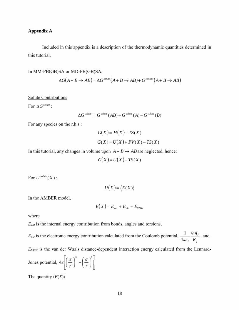
In MM-PB(GB)SA or MD-PB(GB)SA,
( ) ( ) ( )ABBAGABBAGABBAG solventsolute →++→+∆=→+∆
Solute Contributions
For : soluteG∆
)()()( BGAGABGG solutesolutesolutesolute −−=∆
For any species on the r.h.s.:
( ) ( ) )(XTSXHXG −=
( ) )()()( XTSXPVXUXG −+=
In this tutorial, any changes in volume upon ABBA →+ are neglected, hence:
( ) ( ) )(XTSXUXG −=
For : )(XU solute
( ) )(XEXU =
In the AMBER model,
( ) VDWeleval EEEXE ++=
where
Eval is the internal energy contribution from bonds, angles and torsions,
Eele is the electronic energy contribution calculated from the Coulomb potential, ij
ji
Rqq
041
πε, and
EVDW is the van der Waals distance-dependent interaction energy calculated from the Lennard-
Jones potential, ⎥⎥⎦
⎤
⎢⎢⎣
⎡⎟⎠⎞
⎜⎝⎛−⎟
⎠⎞
⎜⎝⎛
612
4rrσσε
The quantity ⟨E(X)⟩
18
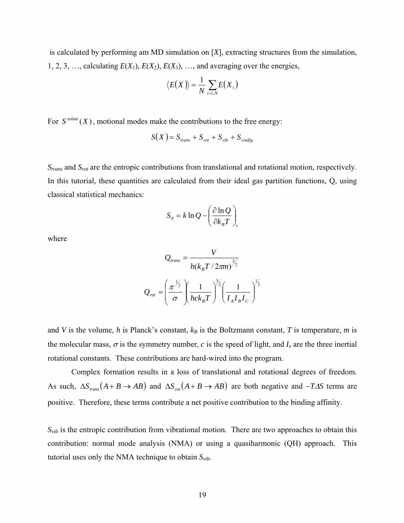
is calculated by performing am MD simulation on [X], extracting structures from the simulation,
1, 2, 3, …, calculating E(X1), E(X2), E(X3), …, and averaging over the energies,
( ) ( )∑=
=Ni
iXEN
XE,1
1
For , motional modes make the contributions to the free energy: )(XS solute
( ) configvibrottrans SSSSXS +++=
Strans and Srot are the entropic contributions from translational and rotational motion, respectively.
In this tutorial, these quantities are calculated from their ideal gas partition functions, Q, using
classical statistical mechanics:
vBTkQQkS ⎟⎟
⎠
⎞⎜⎜⎝
⎛∂∂
−=lnln0
where
23
)2/( mTkh
VQB
transπ
=
21
23
21
11⎟⎟⎠
⎞⎜⎜⎝
⎛⎟⎟⎠
⎞⎜⎜⎝
⎛⎟⎟
⎠
⎞
⎜⎜
⎝
⎛=
CBABrot IIIThck
Qσ
π
and V is the volume, h is Planck’s constant, kB is the Boltzmann constant, T is temperature, m is
the molecular mass, σ is the symmetry number, c is the speed of light, and Ix are the three inertial
rotational constants. These contributions are hard-wired into the program.
Complex formation results in a loss of translational and rotational degrees of freedom.
As such, and ( )ABBAStrans →+∆ ( )ABBASrot →+∆ are both negative and −T∆S terms are
positive. Therefore, these terms contribute a net positive contribution to the binding affinity.
Svib is the entropic contribution from vibrational motion. There are two approaches to obtain this
contribution: normal mode analysis (NMA) or using a quasiharmonic (QH) approach. This
tutorial uses only the NMA technique to obtain Svib.
19
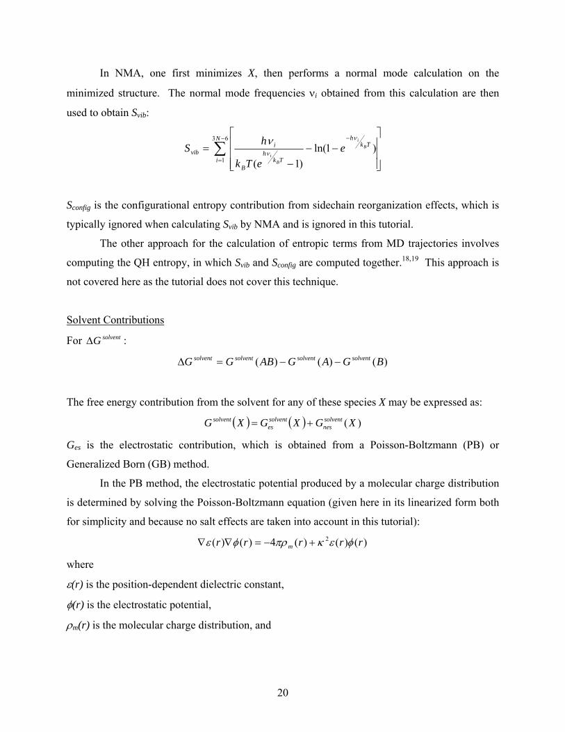
In NMA, one first minimizes X, then performs a normal mode calculation on the
minimized structure. The normal mode frequencies νi obtained from this calculation are then
used to obtain Svib:
∑−
=
−
⎥⎥⎥
⎦
⎤
⎢⎢⎢
⎣
⎡−−
−=
63
1)1ln(
)1(
N
i
Tkh
Tkh
B
ivib
Bi
Bi
eeTk
hS
ν
ν
ν
Sconfig is the configurational entropy contribution from sidechain reorganization effects, which is
typically ignored when calculating Svib by NMA and is ignored in this tutorial.
The other approach for the calculation of entropic terms from MD trajectories involves
computing the QH entropy, in which Svib and Sconfig are computed together.18,19 This approach is
not covered here as the tutorial does not cover this technique.
Solvent Contributions
For : solventG∆
)()()( BGAGABGG solventsolventsolventsolvent −−=∆
The free energy contribution from the solvent for any of these species X may be expressed as:
( ) ( ) )(XGXGXG solventnes
solventes
solvent +=
Ges is the electrostatic contribution, which is obtained from a Poisson-Boltzmann (PB) or
Generalized Born (GB) method.
In the PB method, the electrostatic potential produced by a molecular charge distribution
is determined by solving the Poisson-Boltzmann equation (given here in its linearized form both
for simplicity and because no salt effects are taken into account in this tutorial):
)()()(4)()( 2 rrrrr m φεκπρφε +−=∇∇
where
ε(r) is the position-dependent dielectric constant,
φ(r) is the electrostatic potential,
ρm(r) is the molecular charge distribution, and
20
κ is the Debye-Huckel screening parameter to take into account the electrostatic screening
effects of (monovalent) salt.
Once the electrostatic potential is computed, the electrostatic contribution to the solvation free
energy is given by , where q[ vaciii
i rrq )()( φφ −∑ ] i are the partial atomic charges at positions ri
making up the molecular charge density [ )()( ii
m rrr −= ∑δρ ] and φ(ri)vac is the electrostatic
potential computed for the same charge distribution in vacuum.
In this tutorial, the program DelPhi is used to compute the electrostatic contribution to the
solvation free energy using PB. There is also a PB method implemented in AMBER 8.
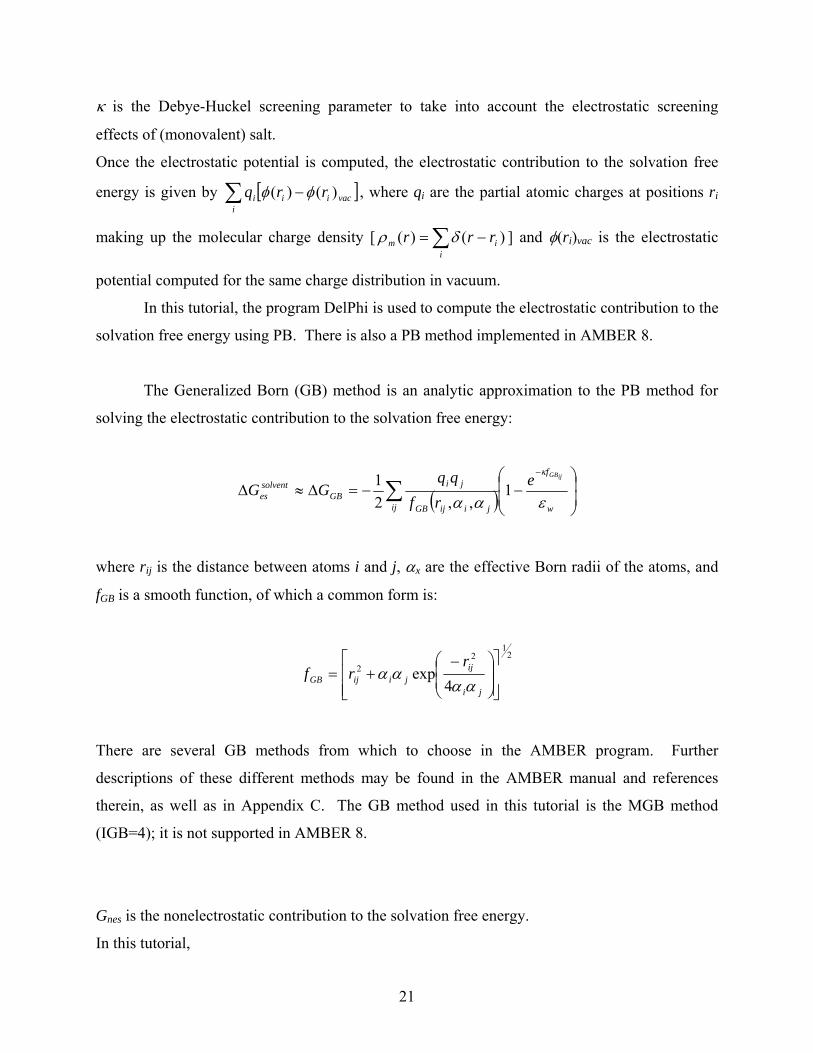
The Generalized Born (GB) method is an analytic approximation to the PB method for
solving the electrostatic contribution to the solvation free energy:
( ) ⎟⎟⎠
⎞⎜⎜⎝
⎛−−=∆≈∆
−
∑w
f
ij jiijGB
jiGB
solventes
ijGBerf
qqGG
εαα
κ
1,,2
1
where rij is the distance between atoms i and j, αx are the effective Born radii of the atoms, and
fGB is a smooth function, of which a common form is:
21
22
4exp
⎥⎥⎦
⎤
⎢⎢⎣
⎡⎟⎟⎠
⎞⎜⎜⎝
⎛ −+=
ji
ijjiijGB
rrf
αααα
There are several GB methods from which to choose in the AMBER program. Further
descriptions of these different methods may be found in the AMBER manual and references
therein, as well as in Appendix C. The GB method used in this tutorial is the MGB method
(IGB=4); it is not supported in AMBER 8.
Gnes is the nonelectrostatic contribution to the solvation free energy.
In this tutorial,
21
( ) ( ) bXSASAXG solventnes += γ
where
γ is a surface tension parameter, set to 0.00542 for PB and 0.0072 for GB in this tutorial,
SASA(X) is the solvent-accessible surface area of molecule X, determined by LCPO or Molsurf in
this tutorial, and
b is a parameterized value, set to 0.92 for PB and 0 for GB in this tutorial.
22
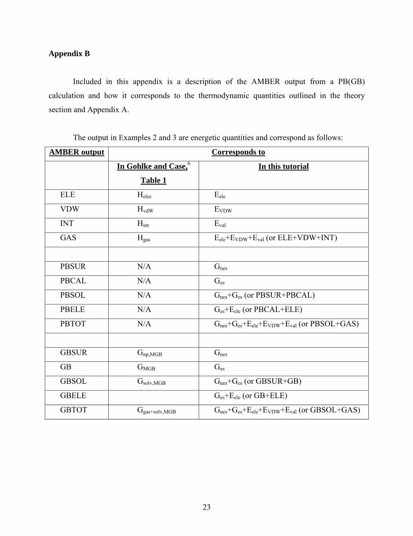
Appendix B
Included in this appendix is a description of the AMBER output from a PB(GB)
calculation and how it corresponds to the thermodynamic quantities outlined in the theory
section and Appendix A.
The output in Examples 2 and 3 are energetic quantities and correspond as follows:
AMBER output Corresponds to
In Gohlke and Case,6
Table 1
In this tutorial
ELE Helec Eele
VDW HvdW EVDW
INT Hint Eval
GAS Hgas Eele+EVDW+Eval (or ELE+VDW+INT)
PBSUR N/A Gnes
PBCAL N/A Ges
PBSOL N/A Gnes+Ges (or PBSUR+PBCAL)
PBELE N/A Ges+Eele (or PBCAL+ELE)
PBTOT N/A Gnes+Ges+Eele+EVDW+Eval (or PBSOL+GAS)
GBSUR Gnp,MGB Gnes
GB GMGB Ges
GBSOL Gsolv,MGB Gnes+Ges (or GBSUR+GB)
GBELE Ges+Eele (or GB+ELE)
GBTOT Ggas+solv,MGB Gnes+Ges+Eele+EVDW+Eval (or GBSOL+GAS)
23
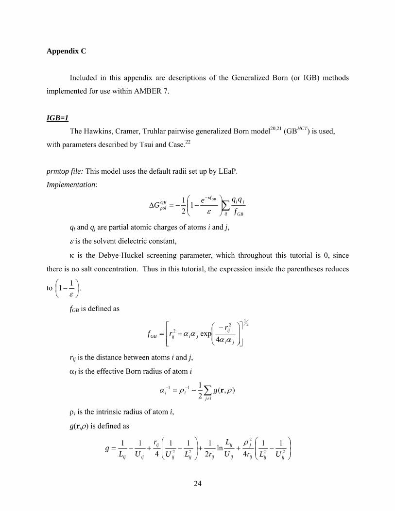
Appendix C
Included in this appendix are descriptions of the Generalized Born (or IGB) methods
implemented for use within AMBER 7.
IGB=1
The Hawkins, Cramer, Truhlar pairwise generalized Born model20,21 (GBHCT) is used,
with parameters described by Tsui and Case.22
prmtop file: This model uses the default radii set up by LEaP.
Implementation:
∑⎟⎟⎠
⎞⎜⎜⎝
⎛−−=∆
−
ij GB
jif
GBpol f
qqeGGB
ε
κ
121
qi and qj are partial atomic charges of atoms i and j,
ε is the solvent dielectric constant,
κ is the Debye-Huckel screening parameter, which throughout this tutorial is 0, since
there is no salt concentration. Thus in this tutorial, the expression inside the parentheses reduces
to ⎟⎠⎞
⎜⎝⎛ −
ε11 .
fGB is defined as
21
22
4exp
⎥⎥⎦
⎤
⎢⎢⎣
⎡⎟⎟⎠
⎞⎜⎜⎝
⎛ −+=
ji
ijjiijGB
rrf
αααα
rij is the distance between atoms i and j,
αi is the effective Born radius of atom i
∑≠
−− −=ij
ii g ),(2111 ρρα r
ρi is the intrinsic radius of atom i,
g(r,ρ) is defined as
⎟⎟⎠
⎞⎜⎜⎝
⎛−++⎟
⎟⎠
⎞⎜⎜⎝
⎛−+−= 22
2
22
114
ln2111
411
ijijij
j
ij
ij
ijijij
ij
ijij ULrUL
rLUr
ULg
ρ
24
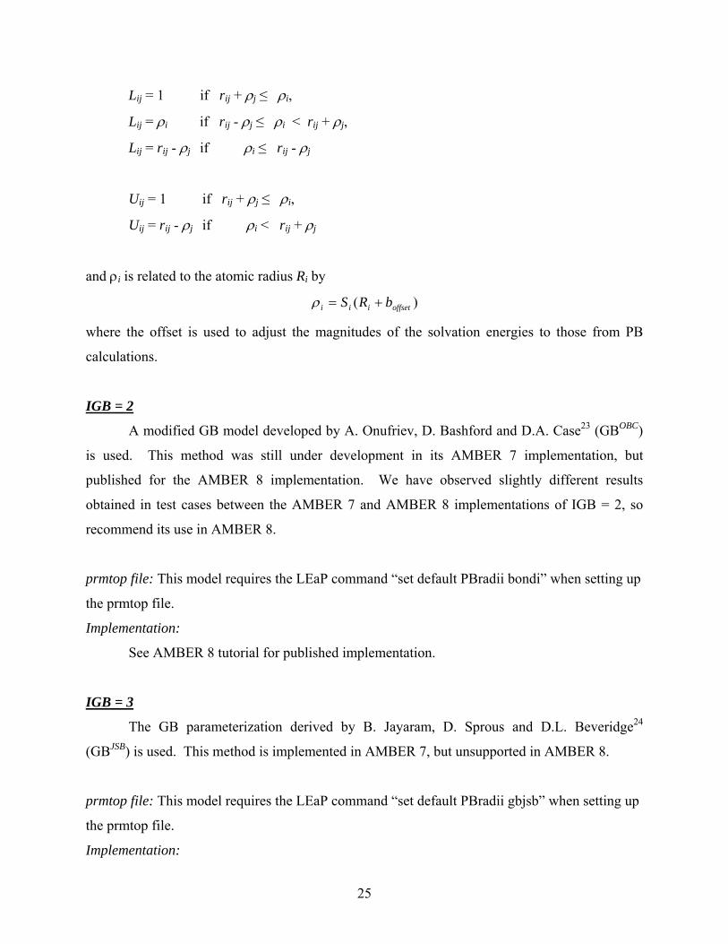
Lij = 1 if rij + ρj ≤ ρi,
Lij = ρi if rij - ρj ≤ ρi < rij + ρj,
Lij = rij - ρj if ρi ≤ rij - ρj
Uij = 1 if rij + ρj ≤ ρi,
Uij = rij - ρj if ρi < rij + ρj
and ρi is related to the atomic radius Ri by
)( offsetiii bRS +=ρ
where the offset is used to adjust the magnitudes of the solvation energies to those from PB
calculations.
IGB = 2
A modified GB model developed by A. Onufriev, D. Bashford and D.A. Case23 (GBOBC)
is used. This method was still under development in its AMBER 7 implementation, but
published for the AMBER 8 implementation. We have observed slightly different results
obtained in test cases between the AMBER 7 and AMBER 8 implementations of IGB = 2, so
recommend its use in AMBER 8.
prmtop file: This model requires the LEaP command “set default PBradii bondi” when setting up
the prmtop file.
Implementation:
See AMBER 8 tutorial for published implementation.
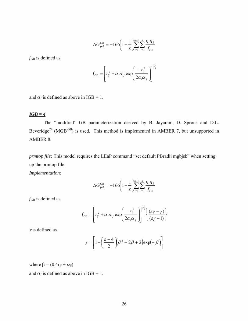
IGB = 3
The GB parameterization derived by B. Jayaram, D. Sprous and D.L. Beveridge24
(GBJSB) is used. This method is implemented in AMBER 7, but unsupported in AMBER 8.
prmtop file: This model requires the LEaP command “set default PBradii gbjsb” when setting up
the prmtop file.
Implementation:
25
∑∑−
= =⎟⎠⎞
⎜⎝⎛ −−=∆
1
1 1
11166n
i
n
j GB
jiGBpol f
qqG
ε
fGB is defined as
21
22
2exp
⎥⎥⎦
⎤
⎢⎢⎣
⎡⎟⎟⎠
⎞⎜⎜⎝
⎛ −+=
ji
ijjiijGB
rrf
αααα
and αi is defined as above in IGB = 1.
IGB = 4
The “modified” GB parameterization derived by B. Jayaram, D. Sprous and D.L.
Beveridge24 (MGBJSB) is used. This method is implemented in AMBER 7, but unsupported in
AMBER 8.
prmtop file: This model requires the LEaP command “set default PBradii mgbjsb” when setting
up the prmtop file.
Implementation:
∑∑−
= =⎟⎠⎞
⎜⎝⎛ −−=∆
1
1 1
11166n
i
n
j GB
jiGBpol f
qqG
ε
fGB is defined as
⎭⎬⎫
⎩⎨⎧
−−
⎥⎥⎦
⎤
⎢⎢⎣
⎡⎟⎟⎠
⎞⎜⎜⎝
⎛ −+=
)1()(
2exp
21
22
εγγεγ
αααα
ji
ijjiijGB
rrf
γ is defined as
( ) ( )⎥⎦
⎤⎢⎣
⎡−++⎟
⎠⎞
⎜⎝⎛ −
−= βββεγ exp222
41 2
where β = (0.4rij + αij)
and αi is defined as above in IGB = 1.
26
Observations/Recommendations:
Gohlke and Case6 found that IGB = 4 predicts the best binding energy compared to
experiment when used in conjunction with the normal mode analysis to obtain entropic terms for
their protein-protein system, Ras-Raf.
In our studies of the protein-RNA system, U1A-RNA, we have observed that IGB = 2
seems to yield the most reasonable overall binding energies in conjunction with normal mode
analysis. The correct trends for the binding energies of mutants is observed by all of the GB
methods, however IGB = 2 performs best, even compared to PB.
27