Embed Size (px)
Citation preview
NBER WORKING PAPER SERIES
RARE BOOMS AND DISASTERS IN A MULTI-SECTOR ENDOWMENT ECONOMY
Jerry TsaiJessica A. Wachter
Working Paper 20062http://www.nber.org/papers/w20062
NATIONAL BUREAU OF ECONOMIC RESEARCH1050 Massachusetts Avenue
Cambridge, MA 02138April 2014
We thank Jonathan Berk, Adlai Fisher, Joao Gomes, Leonid Kogan, Nikolai Roussanov, Harald Uhligand seminar participants at Boston University, McGill University, Stan- ford University, Universityof Miami, University of Pennsylvania, at the American Finance Association Meetings and at the UBCSummer Finance Conference for helpful comments. The views expressed herein are those of the authorsand do not necessarily reflect the views of the National Bureau of Economic Research.
NBER working papers are circulated for discussion and comment purposes. They have not been peer-reviewed or been subject to the review by the NBER Board of Directors that accompanies officialNBER publications.
© 2014 by Jerry Tsai and Jessica A. Wachter. All rights reserved. Short sections of text, not to exceedtwo paragraphs, may be quoted without explicit permission provided that full credit, including © notice,is given to the source.

Rare Booms and Disasters in a Multi-sector Endowment EconomyJerry Tsai and Jessica A. WachterNBER Working Paper No. 20062April 2014, Revised September 2015JEL No. G12
ABSTRACT
Why do value stocks have higher average returns than growth stocks, despite having lower risk? Whydo these stocks exhibit positive abnormal performance while growth stocks exhibit negative abnormalperformance? This paper offers a rare-events based explanation that can also account for the high equitypremium and volatility of the aggregate market. The model explains other puzzling aspects of the datasuch as joint patterns in time series predictablity of aggregate market and value and growth returns,long periods in which growth outperforms value, and the association between positive skewness andlow realized returns.
Jerry TsaiDepartment of EconomicsUniversity of OxfordManor Road BuildingOxford, OX1 [email protected]
Jessica A. WachterDepartment of Finance2300 SH-DHThe Wharton SchoolUniversity of Pennsylvania3620 Locust WalkPhiladelphia, PA 19104and [email protected]

1 Introduction
Among the myriad facts that characterize the cross-section of stock returns, the value
premium stands out both for its empirical robustness and the problem it poses for theory.
The value premium is the finding that stocks with high book-to-market ratios (value)
have higher expected returns than stocks with low book-to-market ratios (growth). By
itself, this finding would not constitute a puzzle, for it could be that value firms are more
risky. Such firms would then have high expected returns in equilibrium, which would
simultaneously explain both their high realized returns and their low valuations. The
problem with this otherwise appealing explanation is that value stocks are not riskier
according to conventional measures. Over the postwar period, which is long enough to
measure second moments, value stocks have lower covariance with the market, and lower
standard deviations. And while one could argue that neither definition of risk is appropriate
in a complex world, the challenge still remains to find a measure of risk that does not, in
equilibrium, essentially amount to covariance or standard deviation. Over a decade of
theoretical research on the value premium demonstrates that this is a significant challenge
indeed.
This paper proposes an explanation of the value premium that is not risk-based but
rather based on rare events. We introduce a representative-agent asset pricing model in
which the endowment is subject to positive and negative events that are much larger than
what would be expected under a normal distribution. One of our theoretical contributions
is to show an asymmetry in how disasters and booms affect average returns. The possibility
of a disaster raises risk premia. While realized returns are lower in samples with disasters
than in those without, these two types of samples are similar in that, in both of them,
an econometrician would calculate a positive disaster premium. The possibility of a boom
also raises risk premia, because it too is a source of risk. Samples with and without booms
look different, however. The econometrician would calculate a positive boom premium in
the first type of sample but a negative boom premium in the second. We use this simple
1

theoretical observation to account for the value premium. In our model, the growth sector
consists of stocks that capture the benefits of a large consumption boom. We show that a
a value premium will be observed if booms were expected but did not occur.
What is the source of the asymmetry between disasters and booms? Why, in other
words, is the measured premium for bearing boom risk positive in population but negative
in samples without rare events? Consider first the case of a risk-neutral investor, and
assume (reasonably) that asset prices rise in booms and fall in disasters. In order to hold
an asset exposed to disasters, the risk-neutral investor must be compensated by higher
realized returns in the event a disaster does not occur. Likewise, when holding an asset
exposed to booms, he is willing to tolerate lower returns in the event the boom does
not occur. If returns were also higher when booms did not occur, no-arbitrage would be
violated.
Now consider the more realistic case of a risk-averse investor. This investor requires a
premium to hold assets exposed to disasters. We would thus expect such assets to have
higher returns, even in samples that contain the “correct” number of disasters. In samples
that, ex post, have no disasters, we would expect these assets to have yet higher returns
because of the no-arbitrage effect discussed in the previous paragraph. As a result, the
econometrician would measure a positive disaster premium in both types of samples: the
true premium is positive, and the observed premium in no-disaster samples is also positive.
As in the case of disasters, the risk-averse investor requires a positive risk premium
to hold assets exposed to booms. However, by no-arbitrage, these assets must have lower
returns in samples where booms do not occur. How can these two statements be reconciled?
It must be that the higher returns due to the risk premium come about when the boom itself
is realized. Samples with and without booms look qualitatively different: assets exposed
to booms have higher true expected returns, but, on average, lower realized returns when
booms do not occur.
This reasoning explains why one should expect to observe a negative premium for boom
risk in samples without rare events. However, it says nothing about the magnitude of the
2

effect. To obtain quantitatively relevant results, a second mechanism is important. In our
model, we make the standard assumption of constant relative risk aversion (CRRA), which
leads to stationary rates of return. This standard assumption also implies that boom risk
has a lower price than disaster risk. Because any risk premium for booms works against our
main mechanism, this second source of asymmetry between disasters and booms combines
with the first to produce an economically significant value premium.
Specifically, in our calibrated model, the average excess market return is 5%. However,
the average return on growth stocks is only 3%, while the average return on value stocks
is 6%. Moreover, our model also explains why value stocks will have strong abnormal
performance, and growth poor abnormal performance relative to the CAPM. The relative
abnormal performance of value stocks implied by our model is 5%, as it is in the data.
Indeed, our model naturally explains aspects of the data on value and growth that have
posed a challenge to previous general equilibrium models. Namely:
1. Growth stocks have higher variance and covariance with the market despite having
lower observed returns.
2. Growth stocks have yet higher covariances with the market, and greater returns than
value stocks, during periods of high market valuations (for example, the late 1990s).
3. The value-minus-growth return, unlike the market excess return, cannot be predicted
by the price-dividend ratio. It can however be predicted by the value spread.
Moreover, while a full explanation of skewness puzzles is outside the scope of this study,
our model does imply that high valuation stocks have high skewness and low expected
returns, as in the data. Our model also implies that assets with high “upside” betas and
low “downside” betas also have low excess returns, as in the data.
In explaining these facts, we tie our hands by assuming that value and growth cash
flows have the same exposure to disaster risk. While differential exposure is plausible and
in the spirit of the model, we assume it away to focus on our main mechanism. Moreover,
3

we assume that booms affect consumption as well as dividends; this implies boom risk is
priced, and this works against us in finding a value premium.
Finally, because of the presence of disasters, the model explains a high equity premium
and equity volatility, along with low volatility of consumption growth. The model achieves
this with a risk aversion coefficient of three. Low risk aversion helps in explaining the value
puzzle in our setting; if risk aversion were too high, growth would carry a higher premium
in population, and we would not be able to match low observed returns over the sample.
The model generates realistic volatility through the mechanism of time-varying disaster and
boom risk, combined with recursive preferences. Without this mechanism, equity claims
would have counterfactually low volatility during normal times.
Thus far the literature has focused on one-sided rare events, namely disasters, to explain
the equity premium. We show however, that the presence of booms has a large affect on the
cross-section if some assets are exposed to them and some are not. That is, by introducing
booms as well as disasters, one can explain not only the equity premium puzzle but the
value puzzle as well.
Relation to the prior literature
In our focus on the underlying dynamics separating value and growth, our model follows a
substantial literature that explicitly models the cash flow dynamics of firms, or sectors, and
how these relate to risk premia in the cross-section (Ai and Kiku (2013), Ai, Croce, and Li
(2013), Berk, Green, and Naik (1999), Carlson, Fisher, and Giammarino (2004), Garleanu,
Kogan, and Panageas (2012), Gomes, Kogan, and Zhang (2003), Kogan, Papanikolaou, and
Stoffman (2013), Novy-Marx (2010), Zhang (2005)). These papers show how endogenous
investment dynamics can lead to a value premium. Ultimately, however, the value premium
arises in these models because of greater risk. Thus these models do not explain the
observed pattern in variances and covariances. A second branch of the literature relates
cash flow dynamics of portfolios, as opposed to underlying firms, to risk premia (Bansal,
Dittmar, and Lundblad (2005), Da (2009), Hansen, Heaton, and Li (2008), Kiku (2006)).
4

This literature finds that dividends on the value portfolio are more correlated with a long-
run component of consumption than dividends and returns on the growth portfolio. In
the context of a model where risk to this long-run component is priced (Bansal and Yaron
(2004)) this covariance leads to a higher premium for value. However, for this long-run
component to be an important source of risk in equilibrium, it also must be present in
the market portfolio, and it must be an important source of variation in these returns
themselves. Again, this would seem to imply, counterfactually, that the covariance with
the market return and volatility of returns would be greater for value than for growth.
Moreover, if the long-run component of consumption growth is an important source of
risk in the market portfolio, consumption growth should be forecastable by stock prices;
however, it is not (Beeler and Campbell (2012)).
To capture the disconnect between risk and return in the cross-section, shocks associated
with growth stocks should have a low price of risk. As shown by Lettau and Wachter
(2007), Santos and Veronesi (2010) and Binsbergen, Brandt, and Koijen (2012), achieving
this pricing poses a challenge for general equilibrium models.1 Kogan and Papanikolaou
(2013) endogenously generate a cross-section of firms through differences in investment
opportunities, but, like Lettau and Wachter, they assume an exogenous stochastic discount
factor. Papanikolaou (2011) does present an equilibrium model in which investment shocks
have a negative price of risk. This is achieved by assuming that the representative agent
has a preference for late resolution of uncertainty. While helpful for explaining the cross-
section, this assumption implies an equity premium that is counterfactually low. In our
model, growth stocks are exposed to a source of risk that with a price that is (endogenously)
small. Nonetheless, our model has a reasonable equity premium.
1Campbell and Vuolteenaho (2004) and Lettau and Wachter (2007) consider the role of duration in
generating a value premium when discount rate shocks carry a zero or negative price. Campbell and
Vuolteenaho use a partial-equilibrium ICAPM while Lettau and Wachter exogenously specify the stochastic
discount factor. McQuade (2013) shows that stochastic volatility in production can generate a value
premium, depending on how the risk of volatility is priced.
5

Our model features rare disasters, as do models of Rietz (1988), Longstaff and Piazzesi
(2004), Veronesi (2004) and Barro (2006). Time-variation in disaster risk is the primary
driver of stock market volatility, and in this our paper is similar to Gabaix (2012), Gourio
(2012) and Wachter (2013). These papers do not study rare booms. Our rare booms are
similar to technological innovations, modeled by Pastor and Veronesi (2009), and Jovanovic
and Rousseau (2003).2 Bekaert and Engstrom (2013) also assume a two-sided risk structure,
but propose a model of the representative agent motivated by habit formation. These
papers do not address the cross-section of stock returns however.
The remainder of the paper is organized as follows. Section 2 describes and solves the
model. Section 3 discusses the model’s quantitative implications for risk and return of value
and growth firms. Section 4 looks at further implications of our model’s mechanism, and
how these fare in the data. Section 5 concludes.
2 Model
2.1 Endowment and preferences
We assume an endowment economy with an infinitely-lived representative agent. Aggregate
consumption (the endowment) follows a diffusion process with time-varying drift:
dCtCt
= µCt dt+ σdBCt, (1)
where BCt is a standard Brownian motion. The drift of the consumption process is given
by
µCt = µC + µ1t + µ2t, (2)
2Pastor and Veronesi (2009) show how the transition from idiosyncratic to systematic risk can explain
time series patterns of returns in innovative firms around technological revolutions. In the present paper, we
assume for simplicity that the risk of the technology is systematic from the start. Jovanovic and Rousseau
(2003) show how technological revolutions can have long-lived effects, in that the firms that capitalize on
such revolutions continue to have high market capitalization in a manner consistent with our model.
6

where
dµjt = −κµjµjtdt+ ZjtdNjt, (3)
for j = 1, 2. Rare events are captured by the Poisson variables Njt. Absent rare events, the
drift rate of consumption is µC and the volatility is σc. This model allows for consumption
to adjust smoothly as in the data (see Nakamura, Steinsson, Barro, and Ursua (2013)), but
yet to undergo periods of extreme growth rates in either direction.
We assume Z1t < 0 and Z2t > 0. Namely, the N1t represents disasters, while N2t
represents booms. Separating disasters and booms in this way will prove useful in the
theoretical results that follow. Let ν1 denote the (time-invariant) disaster distribution and
ν2 the boom distribution. We write Eνj to denote expectations taken over the distribution
νj.
We let λjt denote the intensity of Njt. We will refer to λjt as the probability of rare
event j in what follows; given our calibration, the intensity is a good approximation of the
annual probability. We assume λjt follows the process
dλjt = κλj(λj − λjt) dt+ σλj√λjt dBλjt, j = 1, 2, (4)
where the Bλjt are independent Brownian motions that are each independent of BCt. For
convenience, we now define some vector notation: let λt = [λ1t, λ2t]>, µt = [µ1t, µ2t]
>,
Bλt = [Bλ1t, Bλ2t]> and Bt = [BCt, B
>λt]>.
We assume the continuous-time analogue of the utility function defined by Epstein and
Zin (1989) and Weil (1990), that generalizes power utility to allow for preferences over the
timing of the resolution of uncertainty. The continuous-time version is formulated by Duffie
and Epstein (1992). We assume that the elasticity of intertemporal substitution (EIS) is
equal to one. That is, the utility function Vt for the representative agent is defined using
the following recursion:
Vt = Et
∫ ∞t
f(Cs, Vs) ds, (5)
where
f(Ct, Vt) = β(1− γ)Vt
(logCt −
1
1− γlog((1− γ)Vt)
). (6)
7

The parameter γ represents relative risk aversion and β the rate of time preference. The
assumption of EIS equal to 1 leads to exact expressions that are available in closed-form
up to ordinary differential equations.3
2.2 The state-price density
We start by establishing how the various sources of risk are priced in the economy. We
use the notation Jj(·) to denote how a process changes in response to a rare event of type
j. For example, for the state-price density πt, Jj(πt) = πt − πt− if a type-j jump occurs
at time t. In our complete-markets endowment economy, the state-price density represents
the marginal utility of the representative agent.
Theorem 1. The state-price density πt follows the process
dπtπt−
= µπtdt+ σπtdBt +∑j=1,2
Jj(πt)πt−
dNjt, (7)
where
σπt =[−γσ, bλ1σλ1
√λ1t, bλ2σλ2
√λ2t
], (8)
and
Jj(πt)πt
= ebµjZjt − 1 (9)
bµj =1− γκµj + β
, (10)
bλj =1
σ2λj
(β + κλj −
√(β + κλj
)2 − 2Eνj[ebµjZjt − 1
]σ2λj
), (11)
for j = 1, 2. Moreover, for γ > 1, bλ1 > 0, bλ2 < 0, and bµj < 0 for j = 1, 2.
Proof. See Appendix B.2.
3Using log-linearization, Eraker and Shaliastovich (2008) and Benzoni, Collin-Dufresne, and Goldstein
(2011) find approximate solutions to related continuous-time jump-diffusion models when the EIS is not
equal to one.
8
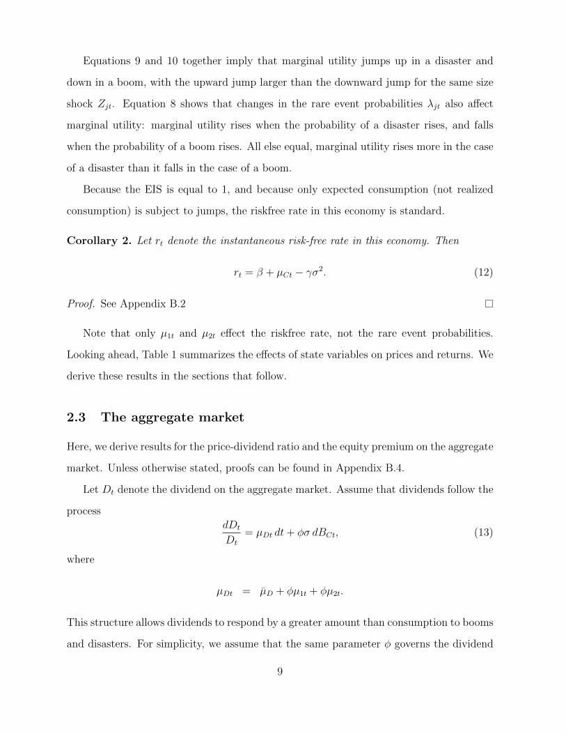
Equations 9 and 10 together imply that marginal utility jumps up in a disaster and
down in a boom, with the upward jump larger than the downward jump for the same size
shock Zjt. Equation 8 shows that changes in the rare event probabilities λjt also affect
marginal utility: marginal utility rises when the probability of a disaster rises, and falls
when the probability of a boom rises. All else equal, marginal utility rises more in the case
of a disaster than it falls in the case of a boom.
Because the EIS is equal to 1, and because only expected consumption (not realized
consumption) is subject to jumps, the riskfree rate in this economy is standard.
Corollary 2. Let rt denote the instantaneous risk-free rate in this economy. Then
rt = β + µCt − γσ2. (12)
Proof. See Appendix B.2
Note that only µ1t and µ2t effect the riskfree rate, not the rare event probabilities.
Looking ahead, Table 1 summarizes the effects of state variables on prices and returns. We
derive these results in the sections that follow.
2.3 The aggregate market
Here, we derive results for the price-dividend ratio and the equity premium on the aggregate
market. Unless otherwise stated, proofs can be found in Appendix B.4.
Let Dt denote the dividend on the aggregate market. Assume that dividends follow the
process
dDt
Dt
= µDt dt+ φσ dBCt, (13)
where
µDt = µD + φµ1t + φµ2t.
This structure allows dividends to respond by a greater amount than consumption to booms
and disasters. For simplicity, we assume that the same parameter φ governs the dividend
9

response to normal shocks, booms and disasters. This φ is analogous to leverage as in Abel
(1999), and we will refer to it as leverage in what follows.
Valuation
Our first result gives the formula for the price of the aggregate market. By no-arbitrage,
F (Dt, µt, λt) = Et
∫ ∞t
πsπtDs ds,
where πs is the state-price density. Valuing the market amounts to calculating the expec-
tation on the right-hand side.
Theorem 3. Let F (Dt, µt, λt) denote the value of the market portfolio. Then
F (Dt, µt, λt) =
∫ ∞0
H (Dt, µt, λt, τ) dτ, (14)
where
H(Dt, µt, λt, τ) = Dt exp{aφ(τ) + bφµ(τ)>µt + bφλ(τ)>λt
}, (15)
bφµj(τ) =φ− 1
κµj
(1− e−κµj τ
), j = 1, 2 (16)
and the remaining terms satisfy
dbφλjdτ
=1
2σ2λjbφλj(τ)2 +
(bλjσ
2λj− κλj
)bφλj(τ) + Eνj
[ebµjZjt
(ebφµj (τ)Zjt − 1
)](17)
daφdτ
= µD − µC − β + γσ2 (1− φ) + bφλ(τ)>(κλ ∗ λ
), (18)
with boundary conditions bφλj(0) = aφ(0) = 0. Furthermore, the price-dividend ratio on the
market portfolio is given by
G(µt, λt) =
∫ ∞0
exp{aφ(τ) + bφµ(τ)>µt + bφλ(τ)>λt
}dτ. (19)
Here and in what follows, bφµ(τ) = [bφµ1(τ), bφµ2(τ)]> and bφλ(τ) = [bφλ1(τ), bφλ2(τ)]>.
Equation 14 expresses the value of the aggregate market as an integral of prices of zero-
coupon equity claims. H gives the values of these claims as functions of the disaster and
10

boom terms µ1t, µ2t, the probabilities of a disaster and boom λ1t, λ2t and the time τ until
the dividend is paid.
These individual dividend prices (and, by extension the price of the market as a whole)
have interpretations based on the primitive parameters. As (16) shows, prices are increasing
in µ1t and µ2t. There is a tradeoff between the effect of expected consumption growth on
future cash flows and on the riskfree rate. Because leverage φ is greater than the EIS
(namely, 1), the cash flow effect dominates and the valuation of the market falls during
disasters and rises during booms. Moreover, the more persistent is the process (the lower
is κµj), the greater is the effect of a change in µjt on prices.4
The probability of rare events also affect prices, but the intuition is more subtle. The
functions bφλ1(τ) and bφλ2(τ) would be identically zero without the last term in the ODE
(17). It is this term that determines the sign of bφλj(τ), and thus how prices respond to
changes in probabilities. We can decompose this last term as follows:
Eνj
[ebµjZjt
(ebφµj (τ)Zjt − 1
)]=
− Eνj[(ebµjZjt − 1
) (1− ebφµj (τ)Zjt
)]︸ ︷︷ ︸
Risk premium effect
+ Eνj
[ebφµj (τ)Zjt − 1
]︸ ︷︷ ︸
Cash flow and riskfree rate effect
. (20)
The first term in (20) is one component of the equity premium, namely, the static rare-event
premium (we discuss this terminology in the next section).5 Because an increase in the
discount rate lowers the price-dividend ratio, this risk premium appears with a negative
sign. The second term is the expected price response if the rare event occurs, representing
the combined effect of changes in expected future cash flows and riskfree rates. Thus the
response of equity values to a change in the rare event probability is determined by a risk
premium effect, and a (joint) cash flow and riskfree rate effect.
These effects have different implications depending on whether the rare event is a dis-
aster or boom. First consider disasters (j = 1). When the risk of a disaster increases, the
4The derivative of (16) with respect to κµj is proportional to (κµjτ + 1)e−κµj τ − 1 which is negative,
because eκµj τ > κµjτ + 1.5More precisely, this is the static rare-event premium for zero-coupon equity with maturity τ .
11
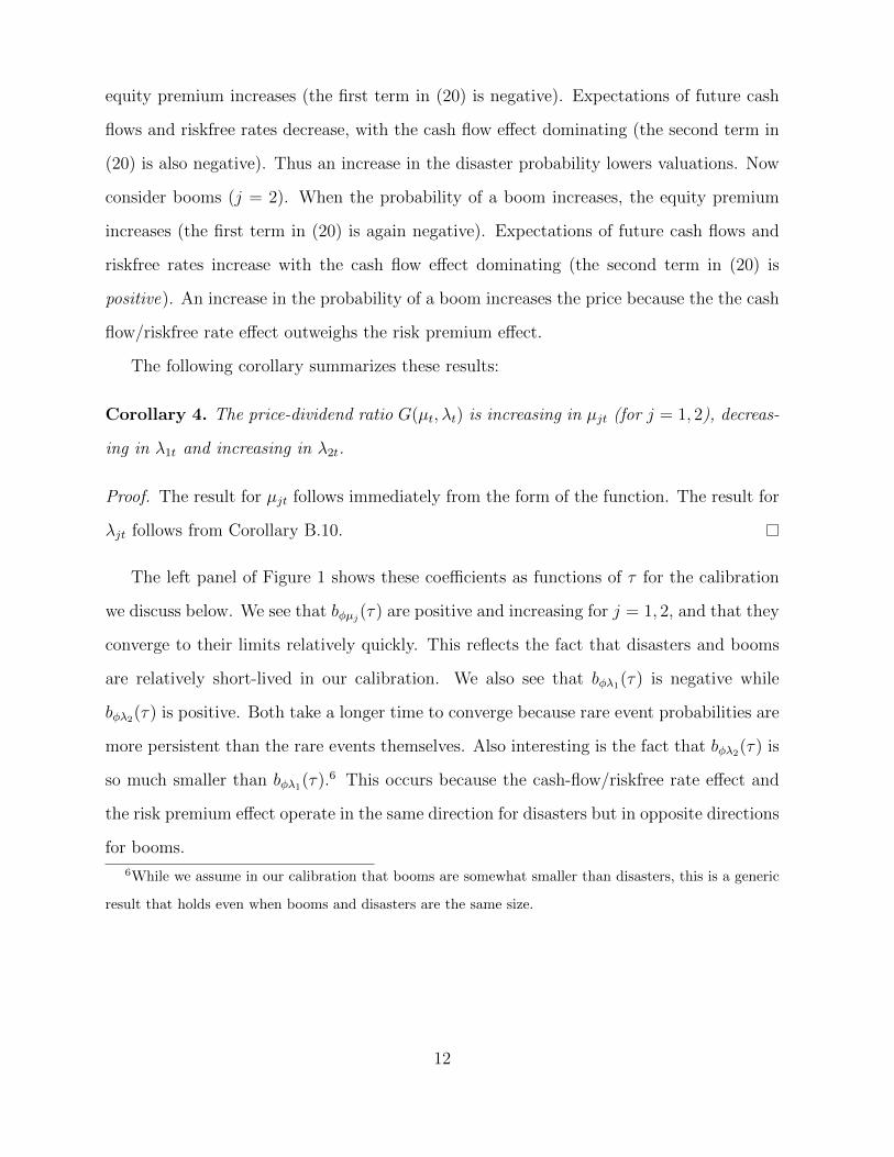
equity premium increases (the first term in (20) is negative). Expectations of future cash
flows and riskfree rates decrease, with the cash flow effect dominating (the second term in
(20) is also negative). Thus an increase in the disaster probability lowers valuations. Now
consider booms (j = 2). When the probability of a boom increases, the equity premium
increases (the first term in (20) is again negative). Expectations of future cash flows and
riskfree rates increase with the cash flow effect dominating (the second term in (20) is
positive). An increase in the probability of a boom increases the price because the the cash
flow/riskfree rate effect outweighs the risk premium effect.
The following corollary summarizes these results:
Corollary 4. The price-dividend ratio G(µt, λt) is increasing in µjt (for j = 1, 2), decreas-
ing in λ1t and increasing in λ2t.
Proof. The result for µjt follows immediately from the form of the function. The result for
λjt follows from Corollary B.10.
The left panel of Figure 1 shows these coefficients as functions of τ for the calibration
we discuss below. We see that bφµj(τ) are positive and increasing for j = 1, 2, and that they
converge to their limits relatively quickly. This reflects the fact that disasters and booms
are relatively short-lived in our calibration. We also see that bφλ1(τ) is negative while
bφλ2(τ) is positive. Both take a longer time to converge because rare event probabilities are
more persistent than the rare events themselves. Also interesting is the fact that bφλ2(τ) is
so much smaller than bφλ1(τ).6 This occurs because the cash-flow/riskfree rate effect and
the risk premium effect operate in the same direction for disasters but in opposite directions
for booms.
6While we assume in our calibration that booms are somewhat smaller than disasters, this is a generic
result that holds even when booms and disasters are the same size.
12

The equity premium
We now turn to the equity premium. For our quantitative results, we will average excess
returns in a simulation, where returns are calculated over a finite time interval that matches
the data. However, we can gain intuition by examining instantaneous (annualized) returns.
By Ito’s Lemma, we can write the price process for the aggregate market as
dFtFt−
= µFt dt+ σFt dBt +∑j=1,2
Jj(Ft)Ft−
dNjt,
for some drift term µFt, a (row) vector of diffusion terms σFt, and termsJj(Ft)Ft−
that denote
percent change in price due to the rare event. Note thatJj(Ft)Ft−
=Jj(Gt)Gt−
, because dividends
themselves do not jump in this model; only the price-dividend ratio does.
The instantaneous expected return is defined as the expected percent price appreciation,
plus the dividend yield. In the notation above,
rmt = µFt +1
Ft
∑j=1,2
λjtEνj [Jt(Ft)]︸ ︷︷ ︸expected price appreciation
+Dt
Ft.︸︷︷︸
dividend yield
(21)
Using this characterization of returns, we can calculate the equity premium.
Theorem 5. The the instantaneous equity premium relative to the risk-free rate rt is
rmt − rt = φγσ2 −∑j=1,2
λjtEνj
[(ebµjZjt − 1
) Jj(Gt)
Gt
]︸ ︷︷ ︸
static rare-event premium
−∑j=1,2
λjt1
Gt
∂G
∂λjbλjσ
2λj︸ ︷︷ ︸
λ-premium
. (22)
Theorem 5 divides the equity premium into three components. The first is the standard
term arising from the consumption CAPM (Breenden (1979)). The second component is the
sum of the premia directly attributable to disasters (j = 1) and to booms (j = 2). These
are covariances between state prices and market returns during rare events, multiplied
by probabilities that the rare events occur.7 We call this second term the static rare
7These terms take the form of uncentered second moments, but they are indeed covariances; this is
because the jump occurs instantaneously and so the conditional expected change in the variable is negligible.
13

event premium because it is there regardless of whether the probabilities of rare events are
constant or time-varying.8
The third component in (22) represents the compensation the investor requires for
bearing the risk of changes in the rare event probabilities. Accordingly, we call this the
λ-premium. This term can also be divided into the compensation for time-varying disaster
probability (the λ1-premium) and compensation for time-varying boom probability (the
λ2-premium). The following corollary shows that all terms in (22) are positive. A closely
related result is that the increases in both the disaster and the boom probability increase
the equity premium, as indicated in Table 1 and discussed in what follows.9
Corollary 6. 1. The static disaster and boom premiums are positive.
2. The premiums for time-varying disaster and boom probabilities (the λj-premiums) are
also positive.
Proof For Result 1, recall that bµj < 0 for j = 1, 2 (Theorem 1). First consider disasters
(j = 1). Note Z1t < 0, so ebµ1Z1t − 1 > 0. Furthermore, because Gt is increasing in µ1t
(Corollary 4), J1(Gt) < 0. It follows that the static disaster premium is positive. Now
consider booms (j = 2). Because Z2t > 0, ebµ2Z2t − 1 < 0. Because Gt is increasing in µ2t,
J2(Gt) > 0. Therefore the static boom premium is also positive.
To show the second statement, first consider disasters (j = 1). Recall that bλ1 > 0
(Theorem 1). Further, ∂G/∂λ1 < 0 (Corollary 4). For booms (j = 2), each of these
quantities takes the opposite sign. The result follows.
8However, the term “static premium” is somewhat of a misnomer, since even the direct effect of rare
events on the price-dividend ratio is a dynamic one. In a model with time-additive utility, only the instan-
taneous co-movement with consumption would matter for risk premia, not changes to the consumption
distribution. Thus there would only be the CCAPM term under our assumptions.9While Table 1 shows that there is no effect of µ1t and µ2t on risk premia, there is in fact a second-
order effect that arises from changes in duration of the claims. This size of this effect is negligible in our
calibration.
14

The static premia are positive because marginal utilities and valuations move in opposite
directions during rare events: during disasters, marginal utility is high, but valuations are
low while during booms the opposite is true. Thus disasters and booms have a direct
positive impact on the equity premium.
Exposure to disasters and booms also increases the equity premium indirectly through
the dynamic effect of time-varying probabilities. An increase in disaster risk raises marginal
utility and lowers valuations, likewise an increase in boom risk lowers marginal utility and
raises market valuations. Thus exposure to time-varying probabilities of rare events further
increases the equity premium.
Figure 2 (top left panel) shows these terms as a function of the disaster probability
for the calibration discussed later in the paper. The dotted line that is essentially at zero
shows the CCAPM. The dash-dotted line shows the static disaster premium; lying above it
is the full static premium, that includes the premium due to booms. Finally, the solid line
is the full equity premium, which includes the λ-premium. While the λ-premium due to
disasters is substantial, the λ-premium due to booms is extremely small. We discuss this
result further in the next section.10
Observed returns in samples without rare events
We now consider the average return the econometrician would observe in an sample without
rare events. To distinguish these average returns from true population returns, we use the
subscript nj (no jump).11 This average return is simply given by the drift rate in the price,
10This figure also shows that the static boom premium is small. This is not a general result; it arises in
our calibration because booms are smaller than disasters. While booms have a smaller effect on marginal
utility and thus on state prices, they have a larger effect on asset prices because of Jensen’s inequality. If
the leverage parameter φ and risk aversion are equal, and booms and disasters are symmetric, then these
terms would be of the same size. On the other hand, the λ-premium due to booms is smaller than for
disasters, even under these conditions.11This “ideal” average return is what one would obtain by averaging over an infinite number of samples
which do not contain rare events.
15

plus the dividend yield:
rmnj,t = µFt +Dt
Ft. (23)
The expression for these average realized returns follows from Theorem 5.
Corollary 7. The average excess market return in a sample without rare events is given
by
rmnj,t − rt = φγσ2 −∑j=1,2
λjtEνj
[ebµjZjt
Jj(Gt)
Gt
]︸ ︷︷ ︸observed static rare-event premium
−∑j=1,2
λjt1
Gt
∂G
∂λjbλjσ
2λj︸ ︷︷ ︸
λ-premium
. (24)
As in the true risk premium, there are components of the observed premium attributable
to disasters (j = 1) and to booms (j = 2). The premium for time-varying λ risk takes the
same form for both the observed and true premium cases, because rare-event risk varies
whether a rare event occurs or not. It is the static premium, or the premium due to the
rare event itself, that differs.12 It follows immediately from (24) (and indeed, it can be
inferred from the definition (23)), that the observed static premium for disasters is higher
than the true static premium, while the observed static premium for booms is lower. In
fact, for booms it will be sufficiently lower so that the observed static premium is negative:
Corollary 8. The observed static disaster premium in a sample without jumps is positive.
The observed static boom premium in a sample without jumps is negative.
Proof The result follows from (24), from ebµjZjt > 0 and from J1(Gt) < 0 and J2(Gt) > 0
(because prices are increasing in µjt).
We now return to a question raised the introduction: why does the average excess return
associated with booms switch signs depending on whether booms are present in the sample?
12We refer to these as the observed premiums to distinguish them from the true risk premiums (note
that, unlike true risk premiums, they do not in fact represent a return for risk). The terminology “observed
static disaster premium” and “observed static boom premium” is used for convenience, not to suggest that
these terms can in fact be observed separately from other parts of the expected excess return in actual
data.
16

Consider first the samples without booms. The intuition in the introduction was based on
no-arbitrage. This intuition is reflected in the very simple proof of Corollary 8. First, the
relevant component of state prices ebµjZjt is positive, regardless of parameter values (this
reflects the absence of arbitrage in the model). Second, during booms, asset prices rise.
The observed (static) boom premium is equal to the negative of the percent change in
asset prices multiplied by the relevant component of the state price. In other words, the
observed premium due to booms must be negative to compensate for the positive returns
when booms are realized; otherwise no-arbitrage would be violated. This effect is mitigated
by risk aversion. The greater is γ, the closer to zero is the observed premium.13 Of course,
as shown in Corollary 6, the true premium due to booms arises from the covariance of state
prices with asset prices and must be positive. This risk premium is realized by the investor
when the boom actually occurs.
We can see the difference between booms and disasters by contrasting the left panels
in Figure 2 with those of Figure 3. Figure 2 shows risk premia as a function of disaster
probability; Figure 3 shows risk premia as a function of boom probability, and hence better
highlights the role of booms. In Figure 2 there is very little difference between true risk
premia and observed risk premia in samples without rare events. In Figure 3, true and
observed risk premia are qualitatively different. The true boom premium is positive, and
increasing in the boom probability, while the observed boom premium is negative, and
decreasing in the probability.
Before leaving the section on risk premia, we note the importance of the asymmetry in
the price of boom versus disaster risk. The discussion above pertains to just the static part
of the premium, not the λ-premium.14 If the λ-premium for booms were large enough it
13More precisely, what matters γ − 1, or more generally, the difference between γ and the inverse of
the EIS. The reason is that the rare events change the consumption distribution rather than consumption
itself. The relevant notion of risk neutrality is thus time-additive utility, in which the agent is indifferent
over the timing of the resolution of uncertainty. In this case, γ = 1 and indeed the static rare-events premia
reduce to price changes.14This raises the question of why we bother making the rare event probabilities vary at all, since the
17

could reduce, or even over-ride our results on the observed static premium. However, the
λ-premium for booms, unlike that for disasters, is negligible. There are two reasons for
this. One is that the price of risk for λ2t is small in magnitude compared to the price of
risk for λ1t, that is bλ1 > −bλ2 . The other is that changes in the probability of boom have
a smaller affect on prices, as explained in the discussion following Theorem 3.
To summarize, this section shows that, while the true premia for both disaster and
boom risk are positive, the observed premium for disaster risk is positive while the observed
premium for boom risk is negative. These results are directly relevant for the cross-section
because, as we will see, value and growth claims differ based on their exposure to these
risks.
2.4 Growth and value sectors
We now turn to the pricing of assets that differ in their exposure to the sources of uncer-
tainty in the economy. See Appendix B.5 for proofs not given below.
The value sector
It makes intuitive sense that firms and industries will differ in their ability to directly profit
from technological progress. For simplicity, we define a sector that does not directly benefit
from a boom, but is otherwise identical to the market. A second sector, one that captures
the benefits of the boom, is simply defined as what remains in the market portfolio after
we subtract the first sector.
Consider an asset with cash flows following the process
dDvt
Dvt
= µvDtdt+ φσdBCt, (25)
where µvDt = µD + φµ1t. We use the superscript v to denote “value”. As we will show, this
main effect in the model does not depend on these terms. The answer is given in the introduction: if
the rare event probabilities were constant, than equity volatility would be essentially zero except when
disasters were to take place.
18

asset will have a lower ratio of price to fundamentals than the market as a whole. This is
the defining characteristic of value in the data.15
Corollary 9. The price-dividend ratio for value is below that of the market.
Dividend growth for the market is weakly greater than dividend growth for value in
every state of the world, and strictly greater in some states of the world. It follows that
the price-dividend ratio, which is the present discounted value of future dividends scaled
by current dividends, is lower for value than for the market.
Pricing for the value claim is directly analogous to that of the market (Theorem 3).
The price of the claim to the dividend stream (25) is given by
F v (Dvt , µt, λt) =
∫ ∞0
Hv (Dvt , µt, λt, τ) dτ, (26)
where
Hv (Dvt , µt, λt, τ) = Dv
t exp{avφ(τ) + bvφµ(τ)>µt + bvφλ(τ)>λt
}. (27)
The price-dividend ratio for the value claim is therefore
Gv(µt, λt) =
∫ ∞0
exp{avφ(τ) + bvφµ(τ)>µt + bvφλ(τ)>λt
}dτ, (28)
with avφ(τ), bvφµ(τ), and bvφλ(τ) given in Appendix B.5. We highlight an important difference
between these terms and their counterparts for the market portfolio. The sensitivity of the
price to booms is given by
bvφµ2(τ) = − 1
κµ2
(1− e−κµ2τ
). (29)
The analogous term for the market is bφµ2(τ) = φ−1κµ2
(1− e−κµ2τ ). From (29), we see that
the price of the value claim fluctuates with booms, even though the cash flow process does
not itself depend on booms. The reason is that, when a boom occurs, the riskfree rate rises
15Our assumptions imply that observed dividend growth is only higher for the growth sector if a rare
boom actually occurs. Thus our model is consistent with the results of Chen (2012), who finds relatively
small differences in the measured growth rate on growth stocks as compared to value stocks.
19
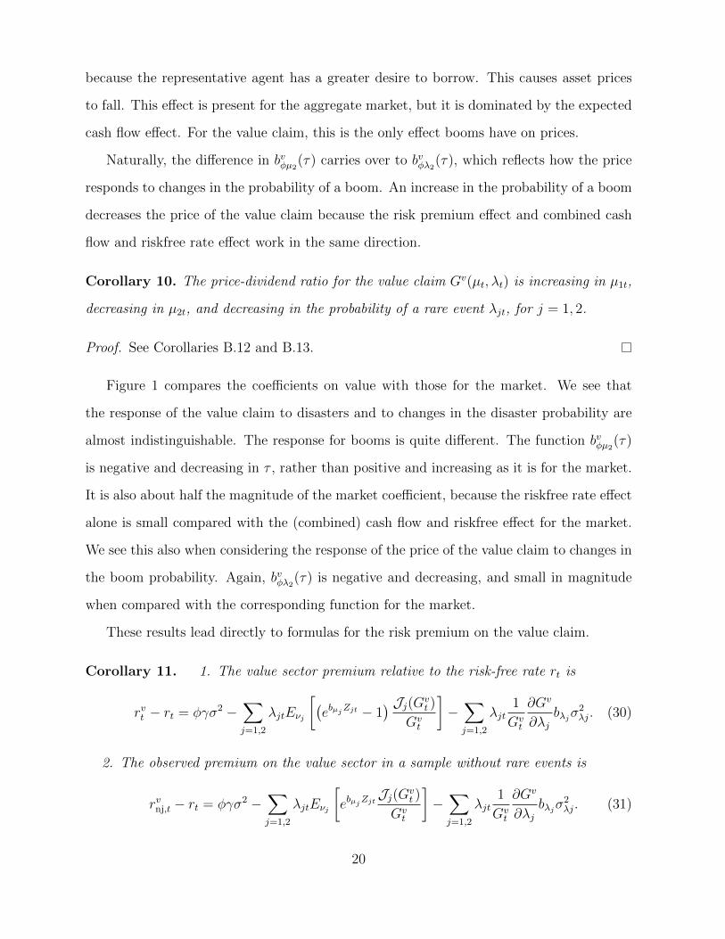
because the representative agent has a greater desire to borrow. This causes asset prices
to fall. This effect is present for the aggregate market, but it is dominated by the expected
cash flow effect. For the value claim, this is the only effect booms have on prices.
Naturally, the difference in bvφµ2(τ) carries over to bvφλ2
(τ), which reflects how the price
responds to changes in the probability of a boom. An increase in the probability of a boom
decreases the price of the value claim because the risk premium effect and combined cash
flow and riskfree rate effect work in the same direction.
Corollary 10. The price-dividend ratio for the value claim Gv(µt, λt) is increasing in µ1t,
decreasing in µ2t, and decreasing in the probability of a rare event λjt, for j = 1, 2.
Proof. See Corollaries B.12 and B.13.
Figure 1 compares the coefficients on value with those for the market. We see that
the response of the value claim to disasters and to changes in the disaster probability are
almost indistinguishable. The response for booms is quite different. The function bvφµ2(τ)
is negative and decreasing in τ , rather than positive and increasing as it is for the market.
It is also about half the magnitude of the market coefficient, because the riskfree rate effect
alone is small compared with the (combined) cash flow and riskfree effect for the market.
We see this also when considering the response of the price of the value claim to changes in
the boom probability. Again, bvφλ2(τ) is negative and decreasing, and small in magnitude
when compared with the corresponding function for the market.
These results lead directly to formulas for the risk premium on the value claim.
Corollary 11. 1. The value sector premium relative to the risk-free rate rt is
rvt − rt = φγσ2 −∑j=1,2
λjtEνj
[(ebµjZjt − 1
) Jj(Gvt )
Gvt
]−∑j=1,2
λjt1
Gvt
∂Gv
∂λjbλjσ
2λj. (30)
2. The observed premium on the value sector in a sample without rare events is
rvnj,t − rt = φγσ2 −∑j=1,2
λjtEνj
[ebµjZjt
Jj(Gvt )
Gvt
]−∑j=1,2
λjt1
Gvt
∂Gv
∂λjbλjσ
2λj. (31)
20

Proof. The result follows from Lemma B.6 and (26). See the proof of Theorem 5 for more
detail.
Corollary 12. 1. The static boom premium for the value sector is negative (it is positive
for the market).
2. The λ2-premium is negative (it is positive for the market).
3. The observed static boom premium for the value sector is positive (it is negative for
the market).
Other components of the risk premium and observed risk premium on value take the
same sign as the market.
Proof. The result follows from Corollary 11 and the same reasoning used to show Corol-
lary 6.
We show the components of the value sector premium next to the market as a function
of disaster probability (Figure 2) and as a function of boom probability (Figure 3). The
difference is most apparent when we consider risk premiums as a function of the boom
probability. For the market portfolio, the static observed boom premium is negative in
samples without rare events. For the value sector, the static observed boom premium
is slightly positive. This reflects the intuition in the introduction: when investors are
expecting booms and they do not occur, the observed returns on assets exposed to booms
will be lower than on assets not exposed to booms (or assets that fall in price when booms
occur). We can see this directly by comparing the left and right figures in Panel B of
Figure 3.
The growth sector
Given this definition of the value sector, the growth sector is defined as the residual. Define
Dgt to be the dividend on the growth claim and F g
t the price. By definition, Dgt = Dt−Dv
t ,
21

and by no-arbitrage,
F gt = Ft − F v
t . (32)
Figure 4 shows dividends (Panel A) and prices (Panel B) for value and for the market in
a typical simulation that contains a boom. The dividend on value is normalized to that of
the market at the start of the simulation. When a boom occurs, a wedge opens up between
the market dividend and the value dividend. This wedge is the dividend on the growth
claim.
Figure 4, Panel B shows the price of a claim to the value sector, the market, and the
growth sector. Though the growth sector pays no dividends prior to the boom, it has a
positive price because investors anticipate the possibility of future dividends. When a boom
occurs, the price of the growth claim immediately rises, the value of the aggregate market
also rises, but by less, and the price of the value claim falls slightly. After the boom, the
price of the growth claim and the overall market remain high relative to value, reflecting
permanently higher dividends.16
We can use the basic accounting identity (32) to derive properties of the growth claim:
Corollary 13. The dividend-price ratio for the growth sector is below the dividend-price
ratio for the value sector.
Proof. It follows from the definition of the growth dividend and from the accounting identity
(32) that
Dgt
F gt
=Dt −Dv
t
Ft − F vt
=Dt −Dv
t
DtGt −DvtG
vt
=1
Gvt
Dt −Dvt
DtGtGvt−Dv
t
. (33)
Note that 1/Gvt is the dividend-price ratio on the value claim. Because value has a lower
16The figure also shows prices of all claims rising after the boom; this is because aggregate dividends are
growing.
22

price-dividend ratio than the market as a whole (Corollary 9), GtGvt
> 1. Furthermore,
Dt > Dvt . Therefore, (Dt −Dv
t )/(DtGtGvt−Dv
t ) < 1. The result follows.
Corollary 14. The price of the growth sector is increasing in µ1, decreasing in λ1, and
increasing in µ2 and λ2.
It is not surprising that the price of the growth claim is increasing in the probability and
expected size of a boom. Less obvious is the fact that growth is also exposed to the risk of a
disaster. Prior to a boom, growth has no cash flows to fall in the case of disaster. However,
after a boom takes place, the cash flows that accrue to growth fall by the same percentage
amount in the event of disaster as the rest of the dividends in the economy. Anticipating
this, investors price the effect of a disaster into growth stocks before the boom occurs.
Finally, a concern one might have with this model is whether the size of the value sector
relative to the market is non-stationary. It might seem that the value sector would grow
ever smaller as a proportion of the market. This would be a problem, as the size of the
value sector in the data does not apear to be trending downward.
It turns out that there is a simple way to avoid the problem of non-stationarity. At
each time t, we assume that a new value sector is created so that the dividend on the value
claim is equal to the dividend of the market.17 The price of this value sector at each time
t is still the no-arbitrage value of the dividend stream (25), and so is equal to (26) with
Dvt = Dt in the first argument.18 Because the price-dividend ratios on value and on the
market are stationary, this normalization yields a stationary value sector. The calculation
of returns is invariant to this normalization, as shown in Appendix C.
The key property of the growth claim that emerges from this section is that it is a
17To be precise, the dividends on the value sector evolve according to
dDvs
Dvs
= µvDsdt+ φσdBCs, s ≥ t (34)
with boundary condition Dvt = Dt.
18Note that Figure 4 shows the time path of prices without redefining value’s dividends; it is therefore
what cash flows and price appreciation look like from the point of view of the owner of each of the claims.
23

levered bet on large booms. Relative to the market as a whole, growth has low value.
However, it bears the entire risk of a boom.
3 Quantitative results
3.1 Data
This section describes our data sources. We will compare our rare events in the model to
tail events in the data, using international consumption data described in detail in Barro
and Ursua (2008). These data contain annual observations on real, per capita consumption
for 43 countries; start dates vary from early in the 19th century to the middle of the 20th
century.
Our aggregate market data come from CRSP. We define the market return to be the
gross return on the value-weighted CRSP index. Dividend growth is computed from the
dividends on this index. The price-dividend ratio is price divided by the previous 12 months
of dividends to remove the effect of seasonality in dividend payments (in computing this
dividend stream, we assume that dividends on the market are not reinvested). We compute
market returns and dividend growth in real terms by adjusting for inflation using changes
in the consumer price index (also available from CRSP). For the government bill rate, we
use real returns on the 3-month Treasury Bill. We also use real, per capital expenditures
on non-durables and services for the U.S., available from the Bureau of Economic Analysis.
These data are annual, begin in 1947, and end in 2010. Focusing on post-war data allows
for a clean comparison between U.S. data and hypothetical samples in which no rare events
take place.
Data on value and growth portfolio are from Ken French’s website. CRSP stocks are
sorted annually into deciles based on their book-to-market ratios. Our growth claim is an
extreme example of a growth stock; it is purely a claim to positive extreme events and
nothing else. In the data, it is more likely that growth stocks are a combination of this
24

claim and the value claim. To avoid modeling complicated share dynamics, we identify
the growth claim with the decile that has the lowest book-to-market ratio, while the value
claim consists of a portfolio (with weights defined by market equity) of the remaining nine
deciles. A standard definition of the value spread is the log book-to-market ratio of the
value portfolio minus the log book-to-market ratio of the growth portfolio (Cohen, Polk,
and Vuolteenaho (2003)). In our endowment economy, book value can be thought of as the
dividend. However, the dividend on the growth claim is identically equal to zero (though
of course this claim has future non-zero dividends), and for this reason, there is no direct
analogue of the value spread. We therefore compute the value spread in the model as the
log dividend-price ratio on the value portfolio minus the log dividend-price ratio on the
aggregate market. For comparability, we use the log book-to-market ratio on value minus
the log book-to-market ratio on the market in the data. Where our non-standard definition
might be an issue is our predictability results; we have checked that these results are robust
to the more standard data definition.
3.2 Calibration
The parameter set consists of the normal-times parameters µC , σ and µD, leverage φ,
the preference parameters β and γ, the parameters determining the duration of disasters
and booms (κµ1 and κµ2 respectively), the parameters determining the disaster and boom
processes (λj, κλj , and σλj for j = 1, 2) and finally the distributions of the disasters
and booms themselves. Some of these parameters define latent processes for which direct
measurement is difficult. The fact that these processes relate to rare events makes the
problem even harder.
For this reason, we proceed by dividing the parameters into groups and impose rea-
sonable restrictions on the parameter space. First, the mean and standard deviation of
consumption growth during normal times are clearly determined by µC and σ. We can
immediately eliminate two free parameters by setting these equal to their values in the
25

postwar data (see Tables 2 and 3).
Second, to discipline to our calibration, we assume that consumption growth after a
disaster reverts to normal at the same rate as consumption growth following a boom,
namely, κµ1 = κµ2 . Further, we assume that the rare event processes are symmetric. That
is, we assume that the average probability of a boom equals that of a disaster (λ1 = λ2),
and that the processes have the same mean reversion and volatility parameters (κλ1 = κλ2
and σλ1 = σλ2).
Third, we calibrate the average disaster probability and the disaster distribution to
international consumption data. Barro and Ursua (2008) estimate that the probability of
a rare disaster in OECD countries is 2.86%.19 We use this number as our average disaster
probability, λ1. Following Barro and Jin (2011), we assume a power law distribution for
rare events (see Gabaix (2009) for a discussion of the properties of power law distributions).
Using maximum likelihood, Barro and Jin estimate a tail parameter of 6.27. They also
argue that the distribution of disasters is better characterized by a double power law, with
a lower exponent for larger disasters. Incorporating this more complicated specification
would lead to a fatter tail and a higher equity premium and volatility. Thus our parameter
choice is conservative.20 Following Barro and Ursua (2008), we assume a 10% minimum
disaster size.
The power law distribution for booms is quite difficult to observe directly. We could
use international data on consumption growth, and in fact such data provide plenty of
evidence of extreme positive growth rates. However, one could reasonably ask whether
19We calibrate the size of the disasters to the full set of countries and the average probability to the
OECD subsample. In both cases, we are choosing the more conservative measure, because the OECD
sub-sample has rarer, but more severe disasters.20One concern is that the consumption data on disasters and booms is international, while our stock
market data is from the U.S. However, many of the facts that we seek to explain have been reported as
robust features of the international data (e.g. Campbell (2003), Fama and French (1992)). We view the
international data as disciplining the choice of distribution of the rare events, as the data from the U.S. is
extremely limited in this regard.
26

these data are directly applicable to a developed country like the United States. We thus
turn to asset markets, and in particular, to the size of the growth sector. The size of the
growth sector in the model turns out to be sensitive to the thickness of the tail of the power
law distribution, a thicker tail implying a larger growth sector. We can therefore infer tail
thickness by matching the size of the growth sector in the model to the size of the growth
sector in the data.21
As discussed in Section 3.1, we identify the growth sector in the model with the lowest
book-to-market decile in the data. We use an annual growth rate of 5% as our minimum
jump size. This would be an unusually high observation for an annual growth rate, so it
is a reasonable choice for the starting point of the upper tail of the consumption growth
distribution. Given this minimum jump size, we require the model to match the relative
book-to-market ratio of value (deciles 2–9) as compared with the market as a whole.22 Given
our other parameter choices, this implies a power law parameter of 15, corresponding to a
thinner tail than for disasters. As we later discuss, it turns out that the value premium is
quite insensitive to the choice of this parameter.
Despite the fact that we use asset market data to infer our distribution for booms, we
still want to compare these booms to those we see in international data. The disaster dis-
tribution and the boom distribution in the model and in the data are reported in Figures 5
and 6. To focus on the tails of the distribution, we consider consumption changes of greater
than 15% for one-year consumption growth rates and consumption changes of greater than
45% for consumption growth rates that are cumulative across five years. These figures
show that, except for small disasters at the five-year horizon, our assumptions imply less
extreme distributions than the data.23 In particular, our model implies fewer, and smaller,
21See, e.g., David and Veronesi (2013) for the use of asset prices to estimate high growth states that may
not have been realized in sample.22In the model, the “book” values of the market and of value are the same. Requiring the model to
match relative market valuations produces very similar answers.23It is the case that our power law distributions are unbounded, thus allowing for small but positive
weight on events that are greater in magnitude than what has occurred in the data. We have checked that
27

booms than observed in the international data.
The remaining parameters are the dividend process parameters µD, and φ, preference
parameters β and γ, and rare event parameters κλ1 = κλ2 and σλ1 = σλ2 . We choose these
parameters to minimize the the distance between the mean value of various statistics in a
sample without rare events and the corresponding statistic in the postwar data. We also
impose some reasonable economic limits on the parameter choices from this search.
The first requirement is that the solution to the agent’s problem exists. It follows from
Theorem 1, that parameters must satisfy
1
2σ2λ1
(κλ1 + β)2 ≥ Eν1
[ebµ1Z1 − 1
](35)
(see also Appendix A). Equation 35 is a joint restriction on the size of a disaster, on the
agent’s risk aversion, on the discount rate of the agent, and on the persistence and volatility
of the disaster probability process.24 Our second requirement is that the discount rate β be
greater than zero. Because of positive consumption growth and a elasticity of intertemporal
substitution equal to 1, matching the low riskfree rate of 1.25 will be a challenge. We discuss
this aspect of the model’s fit in more detail in a later section. We choose a small positive
number for the lower bound of β, and our minimization procedure selects this as optimal
on account of the riskfree rate.
Our third requirement is that leverage (φ) not be “too high”. High leverage helps the
model match the equity premium and volatility, but allowing these data points to determine
φ might lead to a value that is unreasonably high. Cash flow data, on the other hand, does
not clearly pin down a value of φ.25 We choose φ = 3.5, in line with values considered in
the literature (for example, Bansal and Yaron (2004) assume a value of 3.0, while Backus,
truncating the distributions has little effect on the results.24Why, intuitively, is there such a constraint? Note that utility is a solution to a recursive equation;
the above discussion reflects the fact that there is no guarantee in general that a solution to this recursion
exists. In this particular case, it appears that the problematic region of the parameter space is one in which
there is a lot of uncertainty that is resolved very slowly. A sufficiently slow resolution of uncertainty could
lead to infinitely negative utility for our recursive utility agent.25The ratio of dividend to consumption volatility during normal times implies a value of 4.7 (this assumes,
28

Chernov, and Martin (2011) assume a value of 5.1). Given that high values of φ are helpful
for the moments of equity returns, lower values of φ will result in an inferior fit.26
The restrictions above imply that we have three free parameters remaining. We search
over µD, γ, κλ1 as other parameters are determined by these. The moments we use are
average dividend growth, the equity premium, the volatility of the market return, the
average price-dividend ratio and the persistence of the value spread.27 We measure the
model’s fit by simulating 1500 60-year samples and taking only those without rare events.
We minimize the sum of squared differences between the mean across samples and the data
moment, normalizing by the variance across samples. The criterion function is minimized
for average dividend growth µD = 3%, risk aversion γ = 3 and mean reversion κλ1 =
0.11. Value spread moments are reported in Table 4, while aggregate market moments are
reported in Table 5. With these parameters, the probability of not observing a boom in a
60-year period is about 20%. Thus there is no need to assume that the post-war period is
exceptional in that a boom has not been observed.28
however, that dividends are perfectly correlated with consumption in the data). Using the decline in
earnings relative to the decline in consumption during the Great Depression leads to an even higher
number, as earnings fell by nearly 100% (Longstaff and Piazzesi (2004)); however, this decline might have
reasonably been expected by market participants to be temporary, while our model, for simplicity, assumes
such declines are permanent.26We have simulated from a calibration in which the normal-times standard deviation of dividend growth
is twice that of consumption (rather than 3.5 times, as in our benchmark calibration), but where everything
else is the same. The results are very similar to what is reported here, not surprisingly, because it is the
risk of rare events, rather than the normal-times consumption risk, that drives our results. Lowering φ
itself does lead to somewhat lower observed equity and value premia, but the difference is not large. A φ
of 3 implies an equity premium of 5.1% (as compared with 5.4 in our main calibration) and an observed
value premium of 2.6% (as compared with 2.7 in our main calibration).27Attempting to match the very high persistence of the price-dividend ratio leads to unstable results.28Asness, Moskowitz, and Pedersen (2013) report the existence of a value premium in international
equities (Fama and French (1992) also report an international value premium, but over a shorter sample).
The data on individual stocks in Asness et al. come from the U.S., the U.K. and Japan. Given that a large
boom would have worldwide implications, impacting at the least the major developed markets, adding
29

3.3 Simulation results
To evaluate the quantitative succes of the model, we simulate monthly data for 600,000
years, and also simulate 100,000 60-year samples. For each sample, we initialize the λjt
processes using a draw from the stationary distribution.29 Given a simulated series of
the state variables, we obtain price-dividend ratios and one-period dividend growth rates
on the market and on value. Using these quantities we simulate returns as described in
Appendix C. In the tables, we report population values for each statistic, percentile values
from the small-sample simulations, and percentile value for the subset of small-sample
simulations that do not contain rare events. It is this subset of simulations that is the most
interesting comparison for postwar data.
3.3.1 The aggregate market
Table 3 reports moments of log growth rates of consumption and dividends. There is lit-
tle skewness or kurtosis in postwar annual consumption data. Postwar dividend growth
exhibits somewhat more skewness and kurtosis. The simulated paths of consumption and
dividends for the no-jump samples are, by definition, normal, and the results reflect this.
However, the full set of simulations does show significant non-normality; the median kur-
tosis is seven for consumption and dividend growth. Kurtosis exhibits a substantial small-
sample bias. The last column of the table reports the population value of this measure,
which is 55.
Table 5 reports simulation results for the aggregate market. The model is capable of
data from the U.K. and from Japan does not necessarily help us in observing the correct number or size
of the booms. Other data they consider are international equity indices. Our model is a natural fit for
explaining these data as well, since the stock markets of some countries might be expected to outperform
in the event of a large global boom; these would be “growth” according to their measure and would have
lower observed returns. This would also explain the links between the value effects from the international
equity indices and the individual equities.29The stationary distribution for λjt is Gamma with shape parameter 2κj λj/σ
2λj
and scale parameter
σ2λj/(2κj) (Cox, Ingersoll, and Ross (1985)).
30

explaining most of the equity premium: the median value among the simulations with no
disaster risk is 5.4%; in the data it is 7.2%. Moreover, the data value is below the 95th
percentile of the values drawn from the model, indicating that the data value does not reject
the model at the 10% level. The model can also explain high return volatility, and low
volatility of the government bond yield. Note that we define disasters as large deviations
in expected consumption growth. Observed consumption growth is smooth, and it takes
several years for disasters to unfold. Thus the critique of Constantinides (2008), Julliard
and Ghosh (2012) and Mehra and Prescott (1988) concerning the instantaneous nature of
disasters in many models of rare events does not apply here.
Before moving on to the cross-section, we note two limitations to the model’s fit to
the data. First, the average government bond yield in the model is higher than in the
data (1.95% vs. 1.25%). This fit could be improved by allowing a fraction of the disaster
to hit consumption immediately (or a larger fraction than in the present calibration to
hit within the first three months). This effect would be straightforward to implement
but would substantially complicate the notation and exposition without changing any of
the underlying economics. Moreover, Treasury bill returns may in part reflect liquidity
at the very short end of the yield curve (Longstaff (2000)); the model does a better job
of explaining the return on the one-year bond.30 Second, while the model can account
for a substantial fraction of the volatility of the price-dividend ratio (the volatility puzzle,
reviewed in Campbell (2003)), it cannot explain all of it, at least if we take the view that the
postwar series is a sample without rare events. This is a drawback that the model shares
with other models attempting to explain aggregate prices using time-varying moments (see
the discussion in Bansal, Kiku, and Yaron (2012) and Beeler and Campbell (2012)) but
parsimoniously-modeled preferences. It arises from strong general equilibrium effects: time-
varying moments imply cash flow, riskfree rate, and risk premium effects, and one of these
30The model predicts a near-zero volatility for returns on this bill in samples without disasters. This is
not a limitation, since the volatility in returns in the data is due to inflation, which is not captured in the
model.
31

generally acts as an offset to the other two, limiting the effect time-varying moments have
on prices. Some behavior of asset prices (i.e. the “bubble” in the late 1990s) may be beyond
the reach of this type of model. Certainly this is a fruitful area for further research.
3.3.2 Unconditional moments of value and growth portfolios
Tables 6 reports cross-sectional moments in the model. As a “tight” data comparison,
we take the growth portfolio as the bottom decile formed by sorting on book-to-market
and the value portfolio as the remaining nine deciles. This comparison has the advantage
that, in both the model and in the data, the two portfolios considered sum to the market.
However, we also report excess returns for more traditional measures of value and growth
in Table 8.
Table 6 shows that our model can account for an observed value premium of 2.74%, a
substantial fraction of the data value of 4.28%. This value corresponds to the median in
simulations without rare events. The population value premium is negative, as shown in
Section 2. Yet even looking across the full set of simulations implies that it is not unlikely
to observe a value premium in any particular sample.
Table 6 also shows that value stocks have lower standard deviations than growth stocks
and higher Sharpe ratios. Both of these results hold across the full set of simulations,
as well as in the samples without rare events. Both of these affects are strongly present
in the data. The reason the model can capture these effects is that the observed high
average return on value stocks does not represent a return for bearing risk. As explained in
Section 2, because investors are willing to accept a lower return on growth in most periods,
in return for an occasional very high payout.
Perhaps surprisingly, the model’s predictions for the observed value premium are largely
insensitive to the size of booms. In Figure 7, we show the observed value premium for
different specifications of the boom distribution. In Panel A, we vary the probability
of the boom and in Panel B we vary the size of the tail parameter for the power law
distribution. The observed value premium is indeed increasing in the probability of a boom:
32

if the probability of a boom were zero, then so would be the observed value premium.31
Conversely, a high probability of a boom leads to a high observed value premium. In
contrast, Panel B shows that the observed value premium is quite flat as a function of
thickness of the tail. Lower values of the tail parameter imply thicker tails. At extremely
low values expected dividend growth is high enough so that prices fail to converge (see
Assumption 2 in Appendix A). Within the range of 3 to nearly 100, there is little noticeable
change in the observed value premium.
Why is it that the observed value premium is so insensitive to the shape of the boom
distribution? The reason lies with the two opposing forces described in Section 2. On the
one hand, the greater the probability of large booms, the riskier growth stocks become, and
the more negative is the true value premium in population. On the other hand, the greater
the probability of large booms, the lower is the return on growth stocks a risk neutral
investor is willing to accept in samples without booms. These two effects roughly cancel.
Table 6 also shows that our model can explain the relative alphas and betas for value
and growth stocks. Growth stocks have a high covariance with the market, because they
are a levered bet on the occurrence of booms. Shocks to the probability of a boom move the
market price and the growth price in the same direction. The same is true when a boom
actually occurs. Given that growth stocks have higher betas and lower average returns than
value stocks, it is of course not surprising that they have negative alphas. In fact, they
have negative alphas in population as well as in samples without rare events, because a
large part of their risk comes from changes to the probability of a boom, and the premium
associated with this risk is low. Thus, unlike previous models of the value premium, our
model is able to explain the patterns in betas on growth and value in the data.
31We examine the sensitivity across a range from 0.6% probability to 5%. Below this 0.6%, the growth
sector is extremely small and return moments are unstable.
33

3.3.3 Return predictability
In a recent survey, Cochrane (2011) notes that time-varying risk premia are a common
feature across asset classes. However, variables that predict excess returns in one asset
class often fail in another, suggesting that more than one economic mechanism lies behind
this common predictability.32 For example, the price-dividend ratio is a significant predictor
of aggregate market returns, but fails to predict the value-minus-growth return. On the
other hand, the value spread predicts the value-minus-growth return, but it is less successful
than the price-dividend ratio at predicting the aggregate market return.
Panel A of Table 7 shows the results of regressing the aggregate market portfolio return
on the price-dividend ratio in actual and simulated data. The model can reproduce the
finding that the price-dividend ratio predicts excess returns. This result arises primarily
from the fact that a high value of the disaster probability implies a higher equity premium
and a lower price-dividend ratio. It is also the case that a high value of the boom probability
implies a lower return in samples that, ex post, have no booms, as well as a higher price-
dividend ratio. Coefficients and R2 statistics are smaller in a sample with rare events than
without: this is both because more of the variance of stock returns arises from the greater
variance of expected dividend growth during disasters and because the effect of the boom
probability reverses (high premia are associated with high valuations) in the full set of
samples. We can see the effect of small-sample bias (Stambaugh (1999)) by comparing the
population R2 with the median from the full set of simulations.
In the data, the market return can also be predicted by the value spread, though with
substantially smaller t-statistics and R2 values (Panel B of Table 7). The model also
captures the sign and the relative magnitude of this predictability. Compared with the
price-dividend ratio, the value spread is driven more by the time-varying probability of
a boom and less by the probability of a disaster. This explains why risk premia on the
market portfolio, which is mainly driven by the disaster probability, are not captured as
32Lettau and Wachter (2011) show that if a single factor drives risk premia, then population values of
predictive coefficients should be proportional across asset classes.
34

well by the value spread.
Panel C of Table 7 shows that, in contrast to the market portfolio, the value-minus-
growth return cannot be predicted by the price-dividend ratio. The data coefficient is
positive and insignificant. This fact represents a challenge for models that seek to simul-
taneously explain market returns and returns in the cross-section since the forces that
explain time-variation in the equity premium also lead to time-variation in the value pre-
mium (e.g. Lettau and Wachter (2011), Santos and Veronesi (2010)); this reasoning would
lead the coefficient to be negative.33 The present model does, however, predict a positive
coefficient. A high value of the price-dividend ratio on the market mostly reflects a low
probability of a disaster, but also in part a high probability of a boom. If a boom was
expected but did not occur, then average realized returns on value will be high relative to
growth (compare the left and right columns of Panel B, Figure 3).34
One might think that the reason that the value-minus-growth return cannot be predicted
by the price-dividend ratio is that it is not very predictable. This is, however, not the case.
Panel D of Table 7 shows that, as in the data, the value spread predicts the value-minus-
growth return with a positive sign in samples without jumps. The median R2 value at a
1-year horizon is 10%, compared with a data value of 10%. At a 5-year horizon, the value
in the model is 34%, it is 21% in the data. The intuition is the same as for the value-
minus-growth regression on the price-dividend ratio. A high value spread indicates a high
probability of a boom. If we isolate such periods that, ex post, do not have rare events,
growth will have a low return relative to value. The R2 values are much higher than for
the price-dividend ratio because the value spread is primarily driven by the probability of a
33Roussanov (2014) also notes that the conditional mean of the value-minus-growth portfolio does not
vary in the way that univariate models of time-varying risk aversion would predict.34The coefficient is positive in population as well, though it is very small. This arises from a tradeoff
between the effect of the boom probability which gives a negative coefficient (compare the left and right
columns of Panel A in Figure 3), and the effect of disaster probability which predicts a positive one (same
comparison, but in Figure 2),. Value has a slightly lower exposure to disaster probability because of its
shorter duration.
35

boom, while the price-dividend ratio is only driven by this probability to a small extent.35
To summarize, the joint predictive properties of the price-dividend ratio and the value
spread would be quite difficult to explain with a model in which single factor drives risk
premia; they therefore constitute independent evidence of a multiple-factor structure of the
kind presented here.
4 Further implications
4.1 When does growth outperform value?
Our model predicts that in samples when booms are not realized, value stocks will on
average exhibit greater returns than growth stocks. The model also predicts that there will
be periods when growth will outperform value, namely when booms are realized or when
there are positive shocks to the probability of a boom. Both would be expected to occur
during times of substantial technological innovation. How does this prediction fare in the
data? In this section we examine the performance of value and growth during a period
that is indisputably characterized by these shocks, namely the late 1990s.
Table 8 shows statistics for portfolios formed by sorting stocks into quintiles on the basis
of the book-to-market ratio. We examine results for the full CRSP universe, as well as for
the top size quintile. As is well known, value outperforms growth by a substantial margin
over the postwar sample. However, from 1995-2000, the greatest performance belongs to
the lowest book-to-market quintile. Not only do growth stocks exhibit higher returns during
this period, they also have even higher betas than usual. This is evidence in favor of a the
principal mechanism in the model: that growth stocks are more exposed to boom risk than
value stocks.
This exercise naturally raises the question of the differential performance of value and
35In population, the effect works in the opposite direction because high values of the boom probability
predict low returns on value relative to growth. The resulting R2 coefficients are very small. For the set of
all simulations, the mean coefficient is again positive because of small-sample bias.
36

growth during disasters, and during periods when the probability of a disaster increases.
To keep this paper of manageable length, we have not introduced differential exposure of
value and growth dividends to disasters. Considering varying exposure to these shocks,
however, would be within the spirit of the model. We therefore look at the differential
exposure and performance of value and growth during disaster periods.
Panels C and D of Table 8 report the expected returns and betas to value and growth
portfolios during the Great Depression and the financial crisis of 2008 respectively.36 The
table shows that growth has a much lower beta than value during these periods, indicating
that value stocks are more exposed to crises than growth stocks. This is consistent with a
rare events model in which value stocks had greater crisis exposure.37
4.2 Downside and upside risk
Ang, Chen, and Xing (2006) define downside β to be the covariance divided by the variance,
where these moments are computed using only those observations when the market return
is below its mean. Likewise, upside β is the measure when the covariance and variance
are computed for observations when the market return is above its mean. They show that
stocks with higher downside βs have higher returns. Lettau, Maggiori, and Weber (2014)
show that this finding also holds across asset classes.
Ang, Chen, and Xing (2006) also define relative upside and relative downside β to be
the one-sided β measure minus the traditional β. They find that stocks with high relative
downside β have higher mean returns while stocks with high relative upside β have lower
mean returns. Because there are many sources of heterogeneity in stocks that are not
36Our dates are determined from the NBER peak-to-trough measure of the Great Recession.37There are at least two problems with differential exposure to crises as the main explanation of the
value premium. First, if value stocks are more exposed to disasters than growth stocks, they will also have
greater exposure to the probabilities of disasters, and hence counterfactually high betas. This would be
less of a problem if this mechanism were paired with a mechanism like the one we emphasize that lowers
the betas on value stocks. Second, as Table 8 shows, the actual performance of value stocks, outside of the
bottom quintile, was not particularly poor during these periods.
37

captured in the present study, these relative β results seem most relevant.
That there would be a relation between observed one-sided risk and rare events is not
obvious. Disasters and large booms represent extreme one-sided risks that are realized only
rarely. In contrast, the studies mentioned above focus on differential exposure to up- and
down-moves during normal market conditions. However, in the present model there is a
connection because exposure to rare events drives normal-times variation. An asset that
is more exposed to disaster risk will also tend to fall during market downturns, because
a downturn over a finite time interval is more likely to be caused by an increase in the
probability of a disaster than a decrease in the probability of a boom. This effect arises
from the link between the volatility of the rare event probabilities and their magnitudes.
Moreover, while changes in boom probabilities in general have a smaller effect on the market
return than disaster probabilities, upturns will be disproportionately caused by changes in
the boom probability.
Table 9 shows the model’s prediction for the relation between one-sided betas and
expected returns. In the model, value stocks have low relative upside betas, but high
relative downside betas while growth stocks are the opposite. Thus low relative upside
betas and high relative downside betas are associated with high returns, just as in the
data.
4.3 Skewness in the time series and cross-section
Our model predicts that positive skewness should be associated with low future returns,
both in the time series and the cross-section. Several recent papers argue that proxies for
disaster risk predict future returns (Kelly and Jiang (2014), Manela and Moreira (2013)).
Colacito, Ghysels, and Meng (2013) shows that skewness in analysts forecasts, which takes
on both negative and positive values, predicts returns with a negative sign. Like other
papers on disaster risk, this paper predicts that a greater risk of disaster should be associ-
ated with a higher equity premium. It also predicts, consistent with Colacito et al., that a
38

higher chance of a boom will be associated with a lower premium, in a sample where booms
do not occur. Figure 8 shows the skewness conditional on the probability of disasters and
booms. Indeed, skewness is decreasing in the disaster probability and increasing in the
boom probability. Expected returns (in a sample without rare events) go in the opposite
direction.
Measuring skewness whether in the time series or the cross-section, is a challenge. Sev-
eral recent papers, however, are able to calculate ex ante return skewness using option prices
on individual stocks (Conrad, Dittmar, and Ghysels (2013), Chang, Christoffersen, and Ja-
cobs (2013)). These papers show that higher skewness is associated with lower returns in
the cross-section, another prediction of this paper. Conrad, Dittmar, and Ghysels (2013)
also finds that stocks with higher valuation ratios have higher skewness, again consistent
with the results in this paper. Conrad et al. show that stocks with higher book-to-market
ratios have lower coskewness, which is the relevant measure in this paper because booms
are market-wide. They also report that stocks with higher overall skewness have higher
price-to-earnings ratios. These facts are consistent with the finding in this paper that high
valuations are tied to the small probability of very high returns.
5 Conclusion
This paper has addressed the question of how growth stocks can have both low returns and
high risk, as measured by variance and covariance with the market portfolio. It does so
within a framework that is also consistent with what we know about the aggregate market
portfolio; namely the high equity premium, high stock market volatility, and time-variation
in the equity premium. The problem can be broken into two parts: why is the expected
return on growth lower, and why is the abnormal return relative to the CAPM negative?
This latter question is important, because one does not want to increase expected return
through a counterfactual mechanism.
This paper answers the first of these questions as follows: Growth stocks have, in pop-
39

ulation, a slightly higher expected return. In finite samples, however, this return may be
measured as lower. The answer to the second question is different, because the abnor-
mal return relative to the CAPM appears both in population and small samples without
rare events. The abnormal return result arises because risk premia are determined by two
sources of risk, each of which is priced very differently by the representative agent. Co-
variance during disasters, and covariance with the changing disaster probability is assigned
a high price by the representative agent because marginal utility is low in these states.
However, growth stock returns are highly influenced by booms, and by the time-varying
probability of booms. Because marginal utility is low in boom states, the representative
agent requires little compensation for holding this risk. This two-factor structure is also
successful in accounting for the joint predictive properties of the market portfolio and of
the value-minus-growth return.
A number of extensions of the present framework are possible. In this paper, we have
specified the growth and the value claim in a stark manner. Extending our results to a
setting with richer firm dynamics would allow one to answer a broader set of questions.
Further, we have chosen a relatively simple specification for the latent variables driving the
economy. An open question is how the specification of these variables affects the observable
quantities. Finally, we abstract from differential exposure to disaster risk. We leave these
interesting topics to future research.
40

Appendix
A Required conditions on the parameters
Assumption 1. (κλj + β
)2 ≥ 2σ2λjEνj
[ebµjZj − 1
]j = 1, 2.
Assumption 2.
(bλ2σ2λ2− κλ2)2 ≥ 2σ2
λ2Eν2
[ebµ2Z2
(eφ−1κµ2
Z2 − 1
)].
Assumption 3.
µD − µC − β + γσ2 (1− φ)−∑j=1,2
κλj λj
σ2λj
(ζφj − κλj + bλjσ
2λj
)< 0,
where
ζφj =
√(bλjσ
2λj− κλj)2 − 2Eνj
[ebµjZj
(eφ−1κµj
Zj − 1
)]σ2λj.
Assumption 1 is required for the solution for the value function to exist. This restriction
rules out parameters that can lead to infinitely negative utility. Note that for booms,
(assuming relative risk aversion is greater than 1) this restriction is satisfied automatically
since the right hand side is negative.
Assumptions 2 and 3 guarantee convergence of prices, which are given by integrating
expected dividends into the infinite future. Assumption 2 ensures that bφλ2(τ) converges
as τ approaches infinity; namely that the effect of the boom on future dividends cannot
explode as the horizon increases.38 Assumption 3 states that the asymptotic slope of aφ(τ)
is negative. This is the dynamic analogue of the condition that the growth rate be less
than the discount rate in the static Gordon growth model. This condition pertains to the
38Note that no extra assumptions are required for the convergence of bφλ1(τ) because Z1 < 0 and hence
eφ−1κµ1
Z1 < 1. Nor are extra assumptions required for the value function expression bvφλ2(τ) to converge since
this condition replaces eφ−1κµ2
Z2 with e− 1κµ2
Z2 which is less than one.
41

market portfolio. If it is satisfied, the analogous condition for the value claim is satisfied
automatically.39
B Proofs of Theorems
This Appendix contains a detailed solution of the model. Section B.1 describes notation.
Section B.2 describes the derivation of the value function and thus the state-price density
under Assumption 1. Section B.3 contains general results on pricing equities in a model
with jumps. This section does not require parametric assumptions on the processes for
dividends or state prices. Sections B.4 and (most of) B.5 give results under the parametric
assumptions in the main text.
B.1 Notation
• Definition of jump notation J (·):
Let Xt be a pure diffusion process, and let µjt, j = 1, 2 be defined as in (3). Consider
a scalar function h(µ1t, µ2t, Xt). Define
J1(h(µ1t, µ2t, Xt)) = h(µ1 + Z1, µ2, Xt)− h(µ1, µ2, Xt)
J2(h(µ1t, µ2t, Xt)) = h(µ1, µ2 + Z2, Xt)− h(µ1, µ2, Xt).
Further, define
Jj(h(µ1t, µ2t, Xt)) = EνjJj(h(µ1t, µ2t, Xt))
for j = 1, 2, and
J (h(µ1t, µ2t, Xt)) =[J1(h(µ1t, µ2t, Xt)), J2(h(µ1t, µ2t, Xt)
]>.
39Specifically, define
ζvφ2=
√(bλ2
σ2λ2− κλ2
)2 − 2Eν2
[ebµ2Z2
(e− 1κµ2
Z2 − 1)]σ2λ2
Then ζvφ2> ζφ2 . It is also the case that ζvφ1
= ζφ1 .
42

• We use the notation κµ to denote the column vector [κµ1 , κµ2 ]>, and similarly for
κλ, σλ and λ. Recall that we have already defined λt = [λ1t, λ2t]>, µt = [µ1t, µ2t]
>,
Bλt = [Bλ1t, Bλ2t]> and Bt = [BCt, B
>λt]>.
• We use x2 notation for a vector x to denote the square of each element in x. For
example, σ2λ will denote the vector [σ2
λ1, σ2
λ2]>.
• We use the notation ∗ to denote element-by-element multiplication for vectors of the
same dimensionality.
• Partial derivatives with respect to a vector will be assumed to be row vectors. That
is, given a function h(µ), ∂h/∂µ = [∂h/∂µ1, ∂h/∂µ2] , and similarly for λ.
• Because the processes λ are independent, cross-partial derivatives do not enter into
the pricing equations. Thus, given a function h(λ), we use the notation ∂2h/∂λ2 to
denote the row vector [∂2h/∂λ21, ∂
2h/∂λ22].
B.2 The state-price density
As a first step to computing the state-price density, we compute continuation value Vt as
a function of aggregate wealth Wt and the state variables. As is often the case in models
involving square root processes, there are technically two possible solutions corresponding
to the choice of a solution to a quadratic equation. We select the solution such that, when
there is no rare event risk, utility is equivalent to the case when there are in fact no rare
events. Further discussion of this selection procedure is contained in Wachter (2013).
Lemma B.1. In equilibrium, continuation value Vt = J(Wt, µt, λt), where Wt is the wealth
of the representative agent, and J is given as follows:
J(Wt, µt, λt) =W 1−γt
1− γI(µt, λt), (B.1)
where
I(µt, λt) = exp{a+ b>µµt + b>λ λt
}, (B.2)
43

for vectors bµ = [bµ1 , bµ2 ]> and bλ = [bλ1 , bλ2 ]>. The coefficients a, bµj and bλj for j = 1, 2
take the following form:
a =1− γβ
(µC −
1
2γσ2
)+ (1− γ) log β +
1
βb>λ (κλ ∗ λ)
bµj =1− γκµj + β
,
bλj =1
σ2λj
(β + κλj −
√(β + κλj
)2 − 2Eνj[ebµjZjt − 1
]σ2λj
).
Furthermore,
Wt
Ct= β−1. (B.3)
where Ct is aggregate consumption.
Proof Let St denote the value of a claim to aggregate consumption, and conjecture that
the price-dividend ratio for the consumption claim is constant:
StCt
= l,
for some l. This relation implies that St satisfies
dStSt
=dCtCt
= µCt dt+ σ dBCt. (B.4)
Consider an agent who allocates wealth between the claim to aggregate consumption
and the riskfree asset. Let αt be the fraction of wealth in the consumption claim, and let
ct be the agent’s consumption. The wealth process is then given by
dWt =(Wtαt
(µCt − rt + l−1
)+Wtrt − ct
)dt+WtαtσdBct,
where rt denotes the instantaneous riskfree rate. Optimal consumption and portfolio choice
must satisfy the following Hamilton-Jacobi-Bellman (HJB) equation:
supαt,ct
{∂J
∂W
(Wtαt
(µCt − rt + l−1
)+Wtrt − ct
)+∂J
∂λ
(κλ ∗
(λ− λt
))− ∂J
∂µ(κµ ∗ µt)
+1
2
∂2J
∂W 2W 2t α
2tσ
2 +1
2
(∂2J
∂λ2
)(σ2
λ ∗ λt) + λ>t J (J(Wt, µt, λt)) + f (ct, Jt)
}= 0. (B.5)
44

In equilibrium, αt = 1 and ct = Ct = Wtl−1. Substituting these policy functions into
(B.5) implies
∂J
∂WWtµCt +
∂J
∂λ
(κλ ∗
(λ− λt
))− ∂J
∂µ(κµ ∗ µt) +
1
2
∂2J
∂W 2W 2t σ
2
+1
2
(∂2J
∂λ2
)(σ2
λ ∗ λt) + λ>t J (J(Wt, µt, λt)) + f (Ct, Jt) = 0. (B.6)
From the envelope condition ∂f/∂C = ∂J/∂W , we obtain β = l−1, and prove (B.3). Given
that the consumption-wealth ratio equals β−1, it follows that
f(Ct, Vt) = f(Wtl
−1, J (Wt, µt, λt))
= βW 1−γt I (µt, λt)
(log β − log I (µt, λt)
1− γ
), (B.7)
where, to derive (B.7), we conjecture (B.2). Substituting (B.7) and (B.1) into (B.6), we
find
µCt + (1− γ)−1I−1 ∂I
∂λ
(κλ ∗
(λ− λt
))− (1− γ)−1I−1 ∂I
∂µ(κµ ∗ µt)−
1
2γσ2
+1
2(1− γ)−1I−1
(∂2I
∂λ2
)(σ2
λ ∗ λt) + (1− γ)−1λ>t J (I(µt, λt))
+ β
(log β − log I (µt, λt)
1− γ
)= 0.
Note that µCt = µC +µ1t +µ2t. Collecting coefficients on µjt results in linear equations
for bµj for j = 1, 2. Solving these equations yields
bµj =1− γκµj + β
, j = 1, 2.
Collecting coefficients on λjt yields a quadratic equation for bµj for j = 1, 2. Given the root
selection procedure described at the start of this Appendix, the solutions are
bλj =β + κλjσ2λj
−
√√√√(β + κλjσ2λj
)2
−2Eνj
[ebµjZjt − 1
]σ2λj
.
Collecting the constant terms implies
a =1− γβ
(µC −
1
2γσ2
)+ (1− γ) log β +
∑j=1,2
bλjκλjβλj.
This verifies our conjecture on the form of I.
45
Lemma B.2. State prices can be characterized as follows:
πt = exp
{∫ t
0
∂
∂Vf (Cs, Vs) ds
}βγC−γt I(µt, λt) (B.8)
for I(µt, λt) given in Lemma B.1.
Proof Duffie and Skiadas (1994) show that the state-price density πt equals
πt = exp
{∫ t
0
∂
∂Vf (Cs, Vs) ds
}∂
∂Cf (Ct, Vt) . (B.9)
From (6), we obtain
∂
∂Cf (Ct, Vt) = β (1− γ)
VtCt.
Lemma B.1 shows that, in equilibrium, Vt = J (β−1Ct, µt, λt), where the form of J is given
in (B.1). It follows that
∂
∂Cf (Ct, Vt) = βγC−γt I(µt, λt). (B.10)
Equation B.8 then follows from (B.9).
Proof of Theorem 1 We apply Ito’s Lemma to (B.8) to find
dπtπt−
= µπtdt+ σπtdBt +∑j=1,2
Jj(πt)πt−
dNjt,
where
σπt =[−γσ, bλ1σλ1
√λ1t, bλ2σλ2
√λ2t
], (B.11)
and
Jj(πt)πt
= ebµjZjt − 1, for j = 1, 2. (B.12)
Moreover, from Lemma B.1, it follows that a, bµj and bλj take the form described. It follows
immediately that bµj < 0. Because Z1 < 0 and bµ1 < 0, Eν1
[ebµ1Z1t − 1
]> 0. Therefore,√
(β + κλ1)2 − 2Eν1 [ebµ1Z1t − 1]σ2λ1< β + κλ1 .
It follows that bλ1 > 0. Because Z2 > 0 and bµ2 < 0, Eν2
[ebµ2Z2t − 1
]< 0. Therefore,√
(β + κλ2)2 − 2Eν2 [ebµ2Z2t − 1]σ2λ2> β + κλ2
and bλ2 < 0.
46

Proof of Corollary 2 The riskfree rate is obtained by taking the derivative of (B.5) with
respect to αt, evaluating at the equilibrium value of αt = 1 and setting it equal to 0.
Lemma B.3. The drift of the state-price density is given by
µπt = −rt − λ>tJ (πt)
πt(B.13)
= −β − µCt + γσ2 −∑j=1,2
λjtEνj[ebµjZjt − 1
]. (B.14)
Proof Statement (B.13) follows from the absence of arbitrage. Statement (B.14) follows
from Theorem 1, specifically,
λ>tJ (πt)
πt=∑j=1,2
λjtEνj[ebµjZjt − 1
],
and from the expression for rt in Corollary 2.
B.3 General equity pricing results
We first establish a no-arbitrage restriction on the price today of a single dividend payment
in τ periods.
Lemma B.4. Let Ht = H (Dt, µt, λt, τ) denote the time-t price of a single future dividend
payment at time t+ τ :
H(Dt, µt, λt, τ) = Et
[πt+τπt
Dt+τ
]. (B.15)
Then,
dHt
Ht
= µH(τ),tdt+ σH(τ),tdBt +∑j=1,2
Jj(Ht)
Ht
dNjt (B.16)
for scalar processes µH(τ),t and (row) vector processes σH(τ),t. Moreover,
µπt + µH(τ),t + σπtσ>H(τ),t +
1
πtHt
λ>t J (πtHt) = 0. (B.17)
Proof Equation B.16 is a result of Ito’s Lemma and the Markov property of the state
variables and dividends (which implies that H is indeed a function as stated). No-arbitrage
implies
πtH(Dt, λt, µt, T − t) = Et [πsH(Ds, λs, µs, T − s)] for s > t. (B.18)
47

For the remainder of the argument, we simplify notation by writing µHt = µH(τ),t and
σHt = σH(τ),t. Ito’s Lemma applied to πtHt implies
πtHt = π0H0 +
∫ t
0
πsHs
(µHs + µπs + σπsσ
>Hs
)ds+
∫ t
0
πsHs(σHs + σπs)dBs
+∑j=1,2
∑0<sij≤t
(πsijHsij − πs−ijHs−ij
), (B.19)
where sij = inf{s : Njs = i} (namely, the time that the ith type-j jump occurs). Adding
and subtracting the jump compensation term from (B.19) yields:
πtHt = π0H0 +
∫ t
0
πsHs
(µHs + µπs + σπsσ
>Hs +
∑j=1,2
λjJj(πsHs)
πsHs
)ds︸ ︷︷ ︸
(1)
+
∫ t
0
πsHs(σHs + σπs)dBs︸ ︷︷ ︸(2)
+∑j=1,2
∑0<sij≤t
(πsijHsij − πs−ijHs−ij
)−∫ t
0
πsHsλjJj(πsHs)ds
︸ ︷︷ ︸
(3)
. (B.20)
Equation B.18 implies that πtHt is a martingale. Moreover, the terms labeled (2) and (3)
on the right hand side of (B.20) have zero expectation. Therefore the term labeled (1)
must also equal zero in expectation. The process πtHt is strictly positive, and given that
the equation must hold for all t, the integrand must equal zero.
We now prove an extension of Lemma B.4 that holds for the integral of functions H(·, τ)
over τ .
Lemma B.5. Define
F (Dt, µt, λt) =
∫ ∞0
H(Dt, µt, λt, τ) dτ,
assuming this indefinite integral exists. Then
dFtFt−
= µFt dt+ σFt dBt +∑j=1,2
Jj(Ft)Ft−
dNjt, (B.21)
48

for a scalar process µFt and a 1× 3 vector process σFt, satisfying
µπt + µFt +Dt
Ft+ σπtσ
>Ft + λ>t
J (πtFt)
πtFt= 0. (B.22)
Proof First note that (B.21) follows from Ito’s Lemma. We will show (B.22) using the
corresponding result for H, Lemma B.4.40 By applying Ito’s Lemma applied to both F
and H, we find
F (Dt, µt, λt)σFt =
∫ ∞0
H(Dt, µt, λt, τ)σH(τ),t dτ,
and
J (πtF (Dt, µt, λt)) =
∫ ∞0
J (πtH(Dt, µt, λt, τ)) dτ.
Moreover, because H is a function of τ but F is not,
F (Dt, µt, λt)µFt =
∫ ∞0
(H(Dt, λt, µt, τ)µH(τ),t −
∂
∂τH(Dt, µtλt, τ)
)dτ. (B.23)
Equation B.23 can be rigorously derived by applying Ito’s Lemma to F , and differentiating
under the integral sign. Namely,
F (Dt, µt, λt)µFt =
∫ ∞0
(Ht(τ)µDt +
∑j=1,2
∂
∂λjHt(τ)(λj − λj) +
∑j=1,2
∂
∂µjHt(τ)µj +
1
2
∑j=1,2
∂2
∂λ2j
Ht(τ)
)dτ,
where Ht(τ) = H(Dt, µt, λt, τ). We then observe that µH(τ),t is equal to the integrand, plus
∂∂τH(Dt, µtλt, τ).
Finally,
−∫ ∞
0
∂
∂τH(Dt, µt, λt, τ) dτ = H(Dt, µt, λt, 0) = Dt.
The first equality holds because Ht(τ) must equal zero in the limit as τ approaches infinity;
otherwise the indefinite integral would not exist as assumed. The second equality follows
from no-arbitrage. Equation B.22 then follows from Lemma B.4.
Consider the instantaneous expected return described in Section 2.3. Because we only
need to assume a Markov structure, we will use superscript D to denote the fact that
40It is also possible to show (B.22) directly along the same lines as Lemma B.4.
49

we are describing returns on a general dividend claim, as opposed to, say, the market
portfolio. The following lemma contains a convenient and general characterization of the
risk premium in economies with jumps.
Lemma B.6. Let rDt denote the instantaneous expected return
rDt = µFt +Dt
Ft+ λ>t
J (Ft)
Ft. (B.24)
Then
rDt − rt = −σπtσ>Ft −∑j=1,2
λjtEνj
[Jj(Ft)Ft
Jj(πt)πt
]. (B.25)
Proof We start with the result in Lemma B.5, substituting in for µπt using (B.13):
−rt − λ>tJ (πt)
πt︸ ︷︷ ︸µπt
+µFt +Dt
Ft+ σπtσ
>Ft + λ>t
J (πtFt)
πtFt= 0.
We then substitute in for µFt +DtFt
using the definition of rDt , (B.24), and add and subtract
λ>tJ (Ft)Ft
to find
rDt − rt + σπtσ>Ft − λ>t
(J (πt)
πt+J (Ft)
Ft− J (πtFt)
πtFt
)= 0 (B.26)
Finally note that by definition of J ,
Eνj
[Jj(Ft)Ft
Jj(πt)πt
]=Jj(Ftπt)Ftπt
− Jj(Ft)Ft
− Jj(πt)πt
, for j = 1, 2.
The result follows.
B.4 Pricing the aggregate market
We now specialize to the case of the market portfolio as defined in the main text.
Lemma B.7. Assume dividends follow the process (13) with the state-price density de-
scribed in Appendix B.2. The function H, defined in (B.15), takes an exponential form:
H(Dt, µt, λt, τ) = Dt exp{aφ(τ) + bφµ(τ)>µt + bφλ(τ)>λt
}, (B.27)
50
where bφµ = [bφµ1 , bφµ2 ]> and bφλ = [bφλ1 , bφλ2 ]> and
bφµj(τ) =φ− 1
κµj(1− e−κµj τ ), (B.28)
dbφλjdτ
=1
2σ2λjbφλj(τ)2 +
(bλjσ
2λj− κλj
)bφλj(τ) + Eνj
[ebµjZjt
(ebφµj (τ)Zjt − 1
)], (B.29)
daφdτ
= µD − µC − β + γσ2 (1− φ) + bφλ(τ)>(κλ ∗ λ). (B.30)
The boundary conditions are bφλj (0) = aφ (0) = 0.
Proof First note that the boundary conditions follow from H(Dt, µt, λt, 0) = Dt. As ear-
lier, we write Ht = H(Dt, µt, λt, τ) to simplify notation. To prove the remaining statements,
we conjecture the exponential form (B.27). Recall that
dHt
Ht
= µH(τ),tdt+ σH(τ),tdBt +∑j=1,2
Jj(Ht)
Ht
dNjt
as in Lemma B.4. Ito’s Lemma applied to (B.27) implies
Jj(πtHt)
πtHt
= Eνj
[e(bµj+bµjφ(τ))Zjt − 1
], (B.31)
µH(τ),t =1
H
(∂H
∂DµDtDt +
∂H
∂λ(κλ ∗
(λ− λt
))− ∂H
∂µ(κµ ∗ µt)
− ∂H
∂τ+
1
2
(∂2H
∂λ2
)(σ2
λ ∗ λt))
= µDt + bφλ(τ)>(κλ ∗
(λ− λt
))− bφµ(τ)> (κµ ∗ µt)
−(daφdτ
+ λ>tdbφλdτ
+ µ>tdbφµdτ
)+
1
2
(bφλ(τ)2
)> (σ2λ ∗ λt
), (B.32)
and
σH(τ),t =1
H
(∂H
∂D[Dtφσ, 0, 0] +
∂H
∂λ1
[0, σλ1
√λ1t, 0] +
∂H
∂λ2
[0, 0, σλ2
√λ2t]
)=[φσ, bφλ1(τ)σλ1
√λ1t, bφλ2(τ)σλ2
√λ2t
]. (B.33)
51

We now apply Lemma B.4, substituting (B.31–B.33), along with state-price density expres-
sions (8) and (B.14) into the no-arbitrage condition (B.17) to find
µDt + bφλ(τ)>(κλ ∗
(λ− λt
))− bφµ(τ)> (κµ ∗ µt) +
1
2
(bφλ(τ)2
)> (σ2λ ∗ λt
)−γφσ2+bφλ(τ)>
(bλ ∗ σ2
λ ∗ λt)−β−µCt+γσ2(1−φ)+
∑j=1,2
λjtEνj
[e(bµj+bφµj (τ))Zjt − ebµjZjt
]−(daφdτ
+ λ>tdbφλdτ
+ µ>tdbφµdτ
)= 0.
Matching the terms multiplying µj implies
dbφµjdτ
= −κµjbφjµ + (φ− 1) ;
Equation B.28 then follows from the boundary condition. Matching the terms multiplying
λj implies (B.29) and matching the constant terms implies (B.30). This also verifies the
conjectured form for H.
Under our assumptions, the solutions bφλj(τ) have finite limits.
Lemma B.8.
limτ→∞
bφλj(τ) = − 1
σ2λj
(ζφj − κλj + bλjσ
2λj
), (B.34)
where
ζφj =
√√√√(bλjσ2λj− κλj)2 − 2Eνj
[e
(bµj+φ−1
κµj
)Zj − ebµjZj
]σ2λj. (B.35)
Moreover, limτ→∞ bφλ1(τ) < 0 and limτ→∞ bφλ2(τ) > 0.
Proof Let bφλj denote the limit, should it exist. In the limit, small changes in τ do not
change bφλj(τ). Taking the limit of both sides of (17) implies that bφλj must satisfy the
quadratic equation
0 =1
2σ2λjb2φλj
+ (bλjσ2λj− κλj)bφλj + Eνj
[e
(bµj+φ−1
κµj
)Zjt − ebµjZjt
].
52

Equation B.34 gives a solution to this equation.41
To prove that the limits have the signs given in the Lemma, note that Z1 < 0 implies
that
Eν1
[e
(bµ1+φ−1
κµ1
)Z1 − ebµ1Z1
]< 0.
Therefore,
ζφ1 > |bλ1σ2λ1− κλ1|.
Therefore, by (B.34) for j = 1, limτ→∞ bφλ1(τ) < 0
Now, note that Z2 > 0 implies that
Eν2
[e
(bµ2+φ−1
κµ2
)Z2 − ebµ2Z2
]> 0.
Therefore,
ζφ2 < |bλ2σ2λ2− κλ2|
(Assumption 2 implies that ζφ2 is real-valued). Moreover, bλ2 < 0 (Theorem 1), so
0 < ζφ2 < κλ2 − bλ2σ2λ2.
Therefore, by (B.34) for j = 2, limτ→∞ bφλ2(τ) > 0.
While we cannot solve for bφλj(τ) in closed form, we can obtain closed-form solutions
for the related problem of instantaneous disasters. The difference between the equations
is that the last term in (B.29) becomes a constant, rather than a decreasing function of
τ . We can use what we know about the instantaneous-disaster case to put bounds on the
solution for our current case. These bounds allow us to establish monotonicity.
Lemma B.9. Fix τ ∗ > 0. Let b∗φλj(τ) be the solution to
db∗φλjdτ
=1
2σ2λjb∗φλj(τ)2 +
(bλjσ
2λj− κλj
)b∗φλj(τ) + Eνj
[ebµjZjt
(ebφµj (τ∗)Zjt − 1
)](B.36)
41We use the same procedure to select which of the two solutions of the quadratic to use as we used in
Appendix B.2. That is, we chose the one in which rare events do not affect prices if there are in fact no
rare events. We have verified that (B.34) does indeed correspond to the limit when the ordinary differential
equation (17) is solved numerically.
53

with boundary condition b∗φλj(0) = 0. Then b∗φλ1(τ) < bφλ1(τ) < 0 and b∗φλ2
(τ) > bφλ2(τ) > 0
for τ such that 0 < τ < τ ∗.
Proof. Consider j = 1. It follows from (B.29) and the boundary condition that
dbφλ1
dτ
∣∣∣∣τ=0
= 0
d2bφλ1
dτ 2
∣∣∣∣τ=0
< 0
It follows from (B.36) thatdb∗φλ1
dτ
∣∣∣∣τ=0
< 0.
Therefore, because bφλ1(0) = b∗φλ1(0) = 0, there exists τ > 0 but sufficiently small such that
b∗φλ1(τ) < bφλ1(τ) < 0 for τ < τ .
Assume, by contradiction, that there exists a τ < τ ∗ such that bφλ1(τ) ≤ b∗φλ1(τ).
Because bφλ1(τ) and b∗φλ1(τ) are smooth functions, there exists a τ < τ ∗ such that b∗φλ1
(τ) =
bφλ1(τ) and such that b∗φλ1(τ) − bφλ1(τ) is increasing in a neighborhood of τ . However,
because bφµ1(τ ∗)Z1t < bφµ1(τ)Z1t, it follows from (B.36) and (B.29) that
db∗φλ1
dτ
∣∣∣∣τ=τ
<dbφλ1
dτ
∣∣∣∣τ=τ
,
which is a contradiction. Similar reasoning shows that bφλ1(τ) < 0 and the results for
j = 2.42
Corollary B.10. The function bφλ1(τ) is negative and decreasing. The function bφλ2(τ) is
positive and increasing.
Proof. The results bφλ1(τ) < 0 and bφλ2(τ) > 0 are shown in the Lemma above. Consider
j = 1 and fix τ ∗ > 0. Define b∗φλ1(τ) as in Lemma B.9. Because db∗φλ1
/dτ < 0 (see Wachter
(2013)), it follows from (B.36) that
1
2σ2λ1b∗φλ1
(τ)2 +(bλ1σ
2λ1− κλ1
)b∗φλ1
(τ) + Eν1
[ebµ1Z1t
(ebφµ1
(τ∗)Z1t − 1)]< 0. (B.37)
42For j = 2, we need Assumption 2 to guarantee that the function exists and is well-behaved.
54

This inequality must hold for the entire range of values b∗φλ1(τ) for τ between 0 and infinity.
That is,
1
2σ2λ1x2 +
(bλ1σ
2λ1− κλ1
)x+ Eν1
[ebµ1Z1t
(ebφµ1
(τ∗)Z1t − 1)]< 0 x ∈ (inf b∗φλ1
(τ), 0).
Moreover, by Lemma B.9,
inf b∗φλ1(τ) < b∗φλ1
(τ ∗) < bφλ1(τ ∗).
Thus
1
2σ2λ1bφλ1(τ ∗)2 +
(bλ1σ
2λ1− κλ1
)b∗φλ1
(τ ∗) + Eν1
[ebµ1Z1t
(ebφµ1
(τ∗)Z1t − 1)]< 0,
It follows from (B.29) that the left-hand side is equal to dbφλ1/dτ |τ=τ∗ , and therefore that
bφλ1(τ) is a decreasing function of τ . The result follows because τ ∗ is arbitrary. The same
reasoning works for j = 2.
The following lemma shows that the integral determining the price of the market con-
verges. The logic is the similar to that driving the convergence of a geometric sum.
Lemma B.11.
limτ→∞
∫ τ
0
H(D,µ, λ, τ) dτ <∞
for all D > 0, vectors λ with both elements ≥ 0 and all µjt.
Proof Define bφλ2 to be the limit defined in Lemma B.8, and bφµ2 to be the limit of
bφµ2(τ) (the existence of this limit follows immediately from the form of the function). By
Corollary B.10,
H(D,µ, λ, τ) ≤ Debφλ2λ2t+bφµ2
µ2teaφ(τ),
and thus it suffices to show that
limτ→∞
∫ τ
0
eaφ(τ) dτ <∞.
Note that by (18),
aφ(τ) =(µD − µC − β + γσ2 (1− φ)
)τ +
∑j=1,2
κλj λj
∫ τ
0
bφλj(u) du.
55

Now define
aφ = µD − µC − β + γσ2 (1− φ) + bφλ2κλ2λ2.
It follows from the fact that bφλ2(τ) > 0 and is increasing (Corollary B.10) that
aφ(τ) ≤ aφτ + κλ1λ1
∫ τ
0
bφλ1(u) du.
Because bφλ1(τ) is decreasing, by Assumption 3 and by the equations for the limits in
Lemma B.8, there exists a τ0 such that
aφ + bφλ1(τ0)κλ1λ1 < 0.
Write ∫ τ
0
eaφ(τ) dτ ≤∫ τ
0
eaφτ+∫ τ0 bφλ1
(u)κλ1λ1 du dτ
= eaφτ0+∫ τ00 bφλ1
(u)κλ1λ1 du
∫ τ
0
eaφ(τ−τ0)+κλ1
λ1
∫ ττ0bφλ1
(u) dudτ
≤ eaφτ0+∫ τ00 bφλ1
(u)κλ1λ1 du
∫ τ
0
eaφ(τ−τ0)+κλ1λ1bφλ1
(τ0)(τ−τ0) dτ,
where the last line follows from the monotonicity of bφλ1(τ). Convergence as τ →∞ follows
from the properties of the exponential function.
Proof of Theorem 3 Note that, by no-arbitrage,
F (Dt, µt, λt) = Et
∫ ∞t
πsπtDs ds,
assuming the right-hand side is well-defined. It follows from Lemma B.7 thatH(Dt, µt, λt, τ) =
Et
[πt+τπtDτ
]takes the required form. Lemma B.11 shows that the indefinite integral of these
terms exists, and therefore we can write
F (Dt, µt, λt) =
∫ ∞0
H (Dt, µt, λt, τ) dτ.
The equation for the price-dividend ratio follows immediately from dividing this equation
by Dt.
56

Proof of Theorem 5 We use the general formula for the risk premium, given in Lemma B.6:
rmt − rt = −σπtσ>Ft −∑j=1,2
λjtEνj
[Jj(Ft)Ft
Jj(πt)πt
].
It follows from F (Dt, µt, λt) = DtG(µt, λt) and Theorem 3 that
σFt =
[φσ,
1
G
∂G
∂λ1
σλ1
√λ1t,
1
G
∂G
∂λ2
σλ2
√λ2t
].
Because dividends do not jump,
Jj(Ft)Ft−
=Jj(Gt)
Gt−.
Substituting in from (B.11) and (B.12) leads to the equation for the equity premium:
rmt − rt = φγσ2 −∑j=1,2
λjtEνj
[(ebµjZjt − 1
) Jj(Gt)
Gt
]−∑j=1,2
λjt1
Gt
∂G
∂λjbλjσ
2λj.
B.5 Pricing results for value and growth
We first show that the price-dividend ratio for value lies below that of the market. This
result does not depend on our specific assumptions about the dividend process.
Proof of Corollary 9 Consider an asset with dividend stream given by
dDvs
Dvs
= µvDsdt+ φσdBCs,
and µvDs = µD + φµ1s, for s ≥ t, and normalize Dvt to Dt, the dividend on the market.
Comparing the evolution of Dvs with Ds (given in (13)), it follows that
Dvs ≤ Ds for s ≥ t, (B.38)
with a positive probability that the inequality is strict. Therefore, because state prices are
strictly positive,
Et
∫ ∞t
πsπtDvs ds < Et
∫ ∞t
πsπtDs ds.
57

Dividing by Dt implies
Et
∫ ∞t
πsπt
Dvs
Dt
ds < E
∫ ∞t
πsπt
Ds
Dt
ds.
Because Dvt = Dt, the left-hand side is the price-dividend ratio on the value claim. By the
same reason, the right-hand side is the price-dividend ratio on the market.
This result does not require that we define the value claim at time t as an asset having
the same dividend as the market. Normalizing the dividends to be equal is a technical
step within the proof, not an assumption. The price-dividend ratio on the value claim is
determined only by future growth in dividends and in the state-price density, not the level
of current dividends.
It is convenient to state the pricing equations for the value claim. This result follows
from an argument directly analogous to that of Theorem 3.
Corollary B.12. Let F v(Dt, µt, λt) denote the price of the value sector, namely the claim
to cash flows satisfying (25), where Dt is the current dividend.
F v (Dt, µt, λt) =
∫ ∞0
Hv (Dt, µt, λt, τ) dτ. (B.39)
where
Hv(Dt, µt, λt, τ) = Dt exp{avφ(τ) + bvφµ(τ)>µt + bvφλ(τ)>λt
}, (B.40)
bvφµ1(τ) =
φ− 1
κµ1
(1− e−κµ1τ
)(B.41)
bvφµ2(τ) = − 1
κµ2
(1− e−κµ2τ
), (B.42)
while bvφλj(τ) (for j = 1, 2) and aφ(τ) satisfy
dbvφλjdτ
=1
2σ2λjbvφλj(τ)2 +
(bλjσ
2λj− κλj
)bvφλj(τ) + Eνj
[ebµjZjt
(ebvφµj
(τ)Zjt − 1)], (B.43)
davφdτ
= µD − µC − β + γσ2 (1− φ) + bvφλj(τ)>(κλ ∗ λ) (B.44)
with boundary conditions bvφλj(0) = avφ(0) = 0. Furthermore, the price-dividend ratio on the
value sector is given by
Gv(µt, λt) =
∫ ∞0
exp(avφ(τ) + bvφµ(τ)>µt + bvφλ(τ)>λt
)dτ. (B.45)
58
Corollary B.13. The functions bvφλj(τ) are negative and decreasing.
Proof. See Lemma B.9 and Corollary B.10.
We now show that price of the growth claim is increasing in µ1 and µ2, decreasing in
λ1 and increasing in λ2 (Corollary 14 in the main text), using the corresponding results for
the market and the value sector.
Proof of Corollary 14 It follows from the definition of the growth sector price,
F gt = Ft − F v
t ,
that
∂F gt
∂µjt=
∂Ft∂µjt
− ∂F vt
∂µjt(B.46)
and
∂F gt
∂λjt=∂Ft∂λjt
− ∂F vt
∂λjt.
It follows from Corollary 4 that ∂Ft∂µ2t
> 0 and from Corollary 10 that∂F vt∂µ2t
< 0, and similarly
for derivatives with respect to λ2t. Therefore, the price of the growth sector is increasing
in µ2t and λ2t.
Now consider j = 1. Theorem 3 and Corollary B.12 imply that we can rewrite (B.46)
as
∂F gt
∂µjt=
∫ ∞0
bφµ1(τ)H(Dt, µt, λt, τ) dτ −∫ ∞
0
bvφµ1(τ)Hv(Dv
t , µt, λt, τ) dτ.
Moreover, bφµ1(τ) = bvφµ1(τ). Because the dividend at time t+τ on value is less than or equal
to the dividend on the market, and strictly less with positive probability, H(Dt, µt, λt, τ) >
Hv(Dvt , µt, λt, τ). The result follows. The same argument works for the derivative with
respect to λ1t.
59

C Return simulation
This section describes how we simulate returns on the market and the value and growth
sectors, given a simulated series of state variables and one-period observations on dividend
growth. We simulate at a monthly frequency, which is sufficiently fine to capture the joint
distribution of consumption, dividends, and the state variables.
Consider an asset with price process Ft and dividend Dt. The realized return between
time t and t+ ∆t is given by
Rt,t+∆t =Ft+∆t +
∫ t+∆t
tDs ds
Ft
(see Duffie (2001, Chapter 6.L)). Consider an asset that pays a positive dividend at each
point in time (namely, the market or value claim). Using the approximation Dt+∆t∆t ≈∫ t+∆t
tDs ds, we can compute returns as
Rt,t+∆t ≈Ft+∆t +Dt+∆t∆t
Ft
=
Ft+∆t
Dt+∆t+ ∆t
FtDt
Dt+∆t
Dt
=G(µt+∆t, λt+∆t) + ∆t
G(µt, λt)
Dt+∆t
Dt
, (C.1)
where G is the price-dividend ratio on the asset. The price-dividend ratio series is obtained
from the simulated series of state variables using (19) for the market and (28) for value.
Note that this definition of the return makes it unnecessary to have information on either
the level of dividends or the level of prices. Thus this definition is invariant to whether
value is redefined to have the same dividend at time t as the market.
Because the growth sector does not pay a dividend every period, we cannot use (C.1) to
compute its return. However, its return is implied by the fact that the market is a portfolio
of value and growth. Let Rmt,t+∆t denote the market return and Rv
t,t+∆t denote the return
on the value sector, each computed using the relevant quantities in (C.1). Furthermore,
recall that F vt is the price of the value sector at time t and Ft is the price of the market.
60

Then,
Rmt,t+∆t ≈
F vt
FtRvt,t+∆t +
(1− F v
t
Ft
)Rgt,t+∆t. (C.2)
This equation is approximate rather than exact because the model is formulated in contin-
uous time. Solving for the growth return in (C.2) yields
Rgt,t+∆t =
1
1− F vtFt
(Rmt,t+∆t −
F vt
FtRvt,t+∆t
). (C.3)
We now assume that the time-t dividend on value and on the market are the same. It
follows that
F vt
Ft=Gv(µt, λt)
G(µt, λt). (C.4)
Growth returns can then be computed using the state variable series and returns on value
and the market using (C.3) and (C.4).
61

References
Abel, Andrew, 1999, Risk premia and term premia in general equilibrium, Journal of
Monetary Economics 43, 3–33.
Ai, Hengjie, Mariano Massimiliano Croce, and Kai Li, 2013, Toward a Quantitative General
Equilibrium Asset Pricing Model with Intangible Capital, Review of Financial Studies
26, 491–530.
Ai, Hengjie, and Dana Kiku, 2013, Growth to value: Option exercise and the cross section
of equity returns, Journal of Financial Economics 107, 325–349.
Ang, A., J. Chen, and Y. Xing, 2006, Downside Risk, Review of Financial Studies 19,
1191–1239.
Asness, Clifford S., Tobias J. Moskowitz, and Lasse Heje Pedersen, 2013, Value and Mo-
mentum Everywhere: Value and Momentum Everywhere, The Journal of Finance 68,
929–985.
Backus, David, Mikhail Chernov, and Ian Martin, 2011, Disasters Implied by Equity Index
Options, The Journal of Finance 66, 1969–2012.
Bansal, Ravi, Robert F. Dittmar, and Christian T. Lundblad, 2005, Consumption, divi-
dends, and the cross-section of equity returns, Journal of Finance 60, 1639–1672.
Bansal, Ravi, Dana Kiku, and Amir Yaron, 2012, An Empirical Evaluation of the Long-Run
Risks Model for Asset Prices, Critical Finance Review 1, 183–221.
Bansal, Ravi, and Amir Yaron, 2004, Risks for the long-run: A potential resolution of asset
pricing puzzles, Journal of Finance 59, 1481–1509.
Barro, Robert J., 2006, Rare disasters and asset markets in the twentieth century, Quarterly
Journal of Economics 121, 823–866.
62

Barro, Robert J., and Tao Jin, 2011, On the size distribution of macroeconomic disasters,
Econometrica 79, 1567–1589.
Barro, Robert J., and Jose F. Ursua, 2008, Macroeconomic crises since 1870, Brookings
Papers on Economic Activity no. 1, 255–350.
Beeler, Jason, and John Y. Campbell, 2012, The long-run risks model and aggregate asset
prices: An empirical assessment, Critical Finance Review 1, 141–182.
Bekaert, Geert, and Eric Engstrom, 2013, Asset Return Dynamics under Bad Environment
Good Environment Fundamentals, National Bureau of Economic Research, Working
paper 15222.
Benzoni, Luca, Pierre Collin-Dufresne, and Robert S. Goldstein, 2011, Explaining asset
pricing puzzles associated with the 1987 market crash, Journal of Financial Economics
101, 552 – 573.
Berk, Jonathan B., Richard C. Green, and Vasant Naik, 1999, Optimal investment, growth
options, and security returns, Journal of Finance 54, 1553–1607.
Binsbergen, Jules H. van, Michael W. Brandt, and Ralph S. Koijen, 2012, On the timing
and pricing of dividend, American Economic Review 102, 1596–1618.
Breenden, Douglas T., 1979, An intertemporal asset pricing model with stochastic con-
sumption and investment opportunities, Journal of Financial Economics 7, 265–296.
Campbell, John Y., 2003, Consumption-based asset pricing, in G. Constantinides, M. Har-
ris, and R. Stulz, eds.: Handbook of the Economics of Finance, vol. 1b (Elsevier Science,
North-Holland ).
Campbell, John Y., and Tuomo Vuolteenaho, 2004, Bad beta, good beta, American Eco-
nomic Review 94, 1249–1275.
63

Carlson, Murray, Adlai Fisher, and Ron Giammarino, 2004, Corporate investment and
asset price dynamics: Implications for the cross-section of returns, Journal of Finance
59, 2577–2603.
Chang, Bo Young, Peter Christoffersen, and Kris Jacobs, 2013, Market skewness risk and
the cross section of stock returns, Journal of Financial Economics 107, 46–68.
Chen, Huafeng (Jason), 2012, Do Cash Flows of Growth Stocks Really Grow Faster?,
Working paper, University of British Columbia.
Cochrane, John H., 2011, Presidential Address: Discount Rates, The Journal of Finance
66, 1047–1108.
Cohen, Randolph B., Christopher Polk, and Tuomo Vuolteenaho, 2003, The value spread,
Journal of Finance 58, 609–641.
Colacito, Riccardo, Eric Ghysels, and Jinghan Meng, 2013, Skewness in Expected Macro
Fundamentals and the Predictability of Equity Returns: Evidence and Theory, Working
Paper.
Conrad, Jennifer, Robert F. Dittmar, and Eric Ghysels, 2013, Ex Ante Skewness and
Expected Stock Returns, Journal of Finance 68, 85–124.
Constantinides, George M., 2008, Discussion of “Macroeconomic crises since 1870”, Brook-
ings Papers on Economic Activity no. 1, 336–350.
Cox, John C., Jonathan C. Ingersoll, and Stephen A. Ross, 1985, A theory of the term
structure of interest rates, Econometrica 53, 385–408.
Da, Zhi, 2009, Cash Flow, Consumption Risk, and the Cross-section of Stock Returns, The
Journal of Finance 64, 923–956.
David, Alexander, and Pietro Veronesi, 2013, What Ties Return Volatilities to Price Val-
uations and Fundamentals?, Journal of Political Economy 121, 682–746.
64

Duffie, Darrell, 2001, Dynamic Asset Pricing Theory. (Princeton University Press Prince-
ton, NJ) 3 edn.
Duffie, Darrell, and Larry G Epstein, 1992, Asset pricing with stochastic differential utility,
Review of Financial Studies 5, 411–436.
Duffie, Darrell, and Costis Skiadas, 1994, Continuous-time asset pricing: A utility gradient
approach, Journal of Mathematical Economics 23, 107–132.
Epstein, Larry, and Stan Zin, 1989, Substitution, risk aversion and the temporal behavior
of consumption and asset returns: A theoretical framework, Econometrica 57, 937–969.
Eraker, Bjorn, and Ivan Shaliastovich, 2008, An equilibrium guide to designing affine pricing
models, Mathematical Finance 18, 519–543.
Fama, Eugene F., and Kenneth R. French, 1992, The cross-section of expected returns,
Journal of Finance 47, 427–465.
Gabaix, Xavier, 2009, Power laws in economics and finance, Annual review of economics
1, 255–293.
Gabaix, Xavier, 2012, An exactly solved framework for ten puzzles in macro-finance, Quar-
terly Journal of Economics 127, 645–700.
Garleanu, Nicolae, Leonid Kogan, and Stavros Panageas, 2012, Displacement risk and asset
returns, Journal of Financial Economics 105, 491–510.
Gomes, Joao, Leonid Kogan, and Lu Zhang, 2003, Equilibrium cross section of returns,
Journal of Political Economy 111, 693–732.
Gourio, Francois, 2012, Disaster risk and business cycles, American Economic Review 102,
2734–2766.
Hansen, Lars Peter, John C. Heaton, and Nan Li, 2008, Consumption strikes back? Mea-
suring long run risk, Journal of Political Economy 116, 260–302.
65

Jovanovic, Boyan, and Peter L. Rousseau, 2003, Two Technological Revolutions, Journal
of the European Economic Association 1, pp. 419–428.
Julliard, Christian, and Anisha Ghosh, 2012, Can rare events explain the equity premium
puzzle?, The Review of Financial Studies 25, 3037–3076.
Kelly, Bryan, and Hao Jiang, 2014, Tail risk and asset prices, Review of Financial Studies
27, 2841–2871.
Kiku, Dana, 2006, Is the value premium a puzzle?, Working paper, University of Pennsyl-
vania.
Kogan, Leonid, and Dimitris Papanikolaou, 2013, Firm characteristics and stock returns:
The role of investment-specific shocks, Review of Financial Studies 26, 2718–2759.
Kogan, Leonid, Dimitris Papanikolaou, and Noah Stoffman, 2013, Technological innovation:
Winners and losers, National Bureau of Economic Research Working Paper 18671.
Lettau, Martin, Matteo Maggiori, and Michael Weber, 2014, Conditional risk premia in
currency markets and other asset classes, Journal of Financial Economics 114, 197–225.
Lettau, Martin, and Jessica A. Wachter, 2007, Why is long-horizon equity less risky? A
duration-based explanation of the value premium, Journal of Finance 62, 55–92.
Lettau, Martin, and Jessica A. Wachter, 2011, The term structures of equity and interest
rates, Journal of Financial Economics 101, 90 – 113.
Longstaff, Francis A., 2000, Arbitrage and the expectations hypothesis, Journal of Finance
55, 989–994.
Longstaff, Francis A., and Monika Piazzesi, 2004, Corporate earnings and the equity pre-
mium, Journal of Financial Economics 74, 401–421.
Manela, Asaf, and Alan Moreira, 2013, News implied volatility and disaster concerns,
Working paper, Washington University and Yale University.
66

McQuade, Timothy J., 2013, Stochastic Volatility and Asset Pricing Puzzles, Working
paper, Stanford University.
Mehra, Rajnish, and Edward Prescott, 1988, The equity risk premium: A solution?, Journal
of Monetary Economics 22, 133–136.
Nakamura, Emi, Jon Steinsson, Robert Barro, and Jose Ursua, 2013, Crises and recoveries
in an empirical model of consumption disasters, American Economic Journal: Macroe-
conomics 5, 35–74.
Novy-Marx, Robert, 2010, Operating Leverage, Review of Finance 15, 103–134.
Papanikolaou, Dimitris, 2011, Investment Shocks and Asset Prices, Journal of Political
Economy 119, 639–685.
Pastor, Lubos, and Pietro Veronesi, 2009, Technological Revolutions and Stock Prices, The
American Economic Review 99, pp. 1451–1483.
Rietz, Thomas A., 1988, The equity risk premium: A solution, Journal of Monetary Eco-
nomics 22, 117–131.
Roussanov, Nikolai, 2014, Composition of wealth, conditioning information, and the cross-
section of stock returns, Journal of Financial Economics 111, 352–380.
Santos, Tano, and Pietro Veronesi, 2010, Habit formation, the cross section of stock returns
and the cash-flow risk puzzle, Journal of Financial Economics 97, 385–413.
Stambaugh, Robert F., 1999, Predictive regressions, Journal of Financial Economics 54,
375–421.
Veronesi, Pietro, 2004, The Peso problem hypothesis and stock market returns, Journal of
Economic Dynamics and Control 28, 707–725.
Wachter, Jessica A., 2013, Can time-varying risk of rare disasters explain aggregate stock
market volatility?, The Journal of Finance 68, 987–1035.
67

Weil, Philippe, 1990, Nonexpected utility in macroeconomics, Quarterly Journal of Eco-
nomics 105, 29–42.
Zhang, Lu, 2005, The value premium, Journal of Finance 60, 67–103.
68
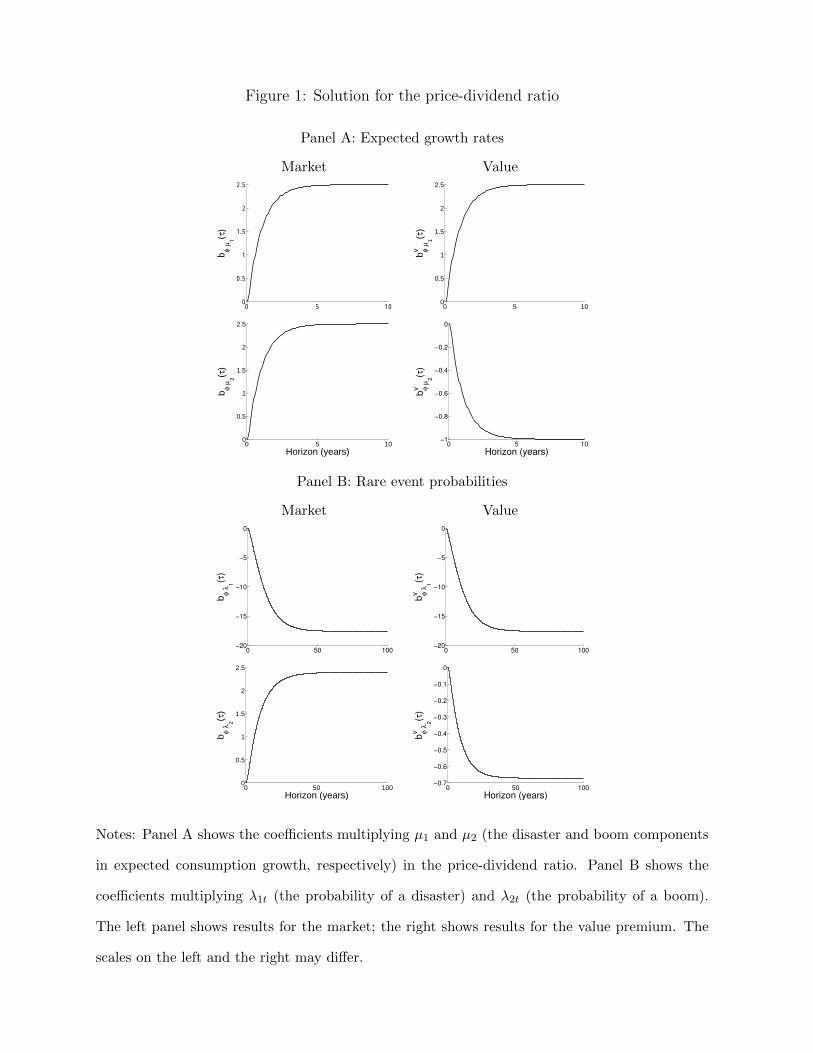
Figure 1: Solution for the price-dividend ratio
Panel A: Expected growth rates
Market Value
0 5 100
0.5
1
1.5
2
2.5
bφ µ
1
(τ)
0 5 100
0.5
1
1.5
2
2.5
bv φ µ
1
(τ)
0 5 100
0.5
1
1.5
2
2.5
Horizon (years)
bφ µ
2
(τ)
0 5 10−1
−0.8
−0.6
−0.4
−0.2
0
Horizon (years)
bv φ µ
2
(τ)
Panel B: Rare event probabilities
Market Value
0 50 100−20
−15
−10
−5
0
bφ λ
1
(τ)
0 50 100−20
−15
−10
−5
0
bv φ λ
1
(τ)
0 50 1000
0.5
1
1.5
2
2.5
bφ λ
2
(τ)
Horizon (years)0 50 100
−0.7
−0.6
−0.5
−0.4
−0.3
−0.2
−0.1
0
Horizon (years)
bv φ λ
2
(τ)
Notes: Panel A shows the coefficients multiplying µ1 and µ2 (the disaster and boom components
in expected consumption growth, respectively) in the price-dividend ratio. Panel B shows the
coefficients multiplying λ1t (the probability of a disaster) and λ2t (the probability of a boom).
The left panel shows results for the market; the right shows results for the value premium. The
scales on the left and the right may differ.

Figure 2: Risk premiums as a function of disaster probability
Market Value
Panel A: Population
0
5
10
15
20
25
annual pre
miu
m (
%)
total premium
static rare event premium
static disaster premium
CCAPM
Panel B: In a sample without rare events
0 0.02 0.04 0.06 0.08
0
5
10
15
20
25
annual pre
miu
m (
%)
disaster probability0 0.02 0.04 0.06 0.08
disaster probability
Notes: Panel A shows population risk premia as functions of the disaster probability with the boom
probability fixed at its mean. The vertical line represents the mean of the disaster probability.
Panel B shows what the average realized excess return would be in a sample without rare events.

Figure 3: Risk premiums as a function of boom probability
Market Value
Panel A: Population
−4
−2
0
2
4
6
8
10
annual pre
miu
m (
%)
Panel B: In a sample without rare events
0 0.02 0.04 0.06 0.08−4
−2
0
2
4
6
8
10
annual pre
miu
m (
%)
boom probability0 0.02 0.04 0.06 0.08
boom probability
total premium
static rare event premium
static boom premium
CCAPM
Notes: Panel A shows population risk premia as functions of the boom probability with the disaster
probability fixed at its mean. The vertical line represents the mean of the boom probability.
Panel B shows what the average realized excess return would be in a sample without rare events.

Figure 4: Sample simulation path of asset dividends and prices
0 5 10 15 200
0.5
1
1.5
2
2.5
Time (years)
Div
idend
Market
Value
Growth
0 5 10 15 200
10
20
30
40
50
60
70
Time (years)
Price
Market
Value
Growth
Notes: This figure shows results from a time series simulated from the model that includes
a boom. The top figure shows dividends (initialized at one), while the bottom panel shows
prices. The solid line marks the onset of the boom.

Figure 5: Tails of the one-year consumption growth rate distribution
Panel A: Model
Disaster Boom
−80 −60 −40 −200
0.0025
0.005
0.0075
0.01
0.0125
Fre
quency o
f events
20 40 600
0.0025
0.005
0.0075
0.01
0.0125
Panel B: Data
−80 −60 −40 −200
0.0025
0.005
0.0075
0.01
0.0125
Realized consumption growth (%)
Fre
quency o
f E
vents
20 40 600
0.0025
0.005
0.0075
0.01
0.0125
Realized consumption growth (%)
Note: This figure shows histograms of one-year consumption growth rates. The right panel
considers growth rates above 15%. The left panel considers growth rates below -15%. The
frequency is calculated by the number of observations within a range, divided by the total
number of observations in the sample. Panel A shows results from simulated data from the
model. Panel B shows results from the data. Data are from Barro and Ursua (2008). For
the consumption booms, we exclude observations between 1944 and 1953.
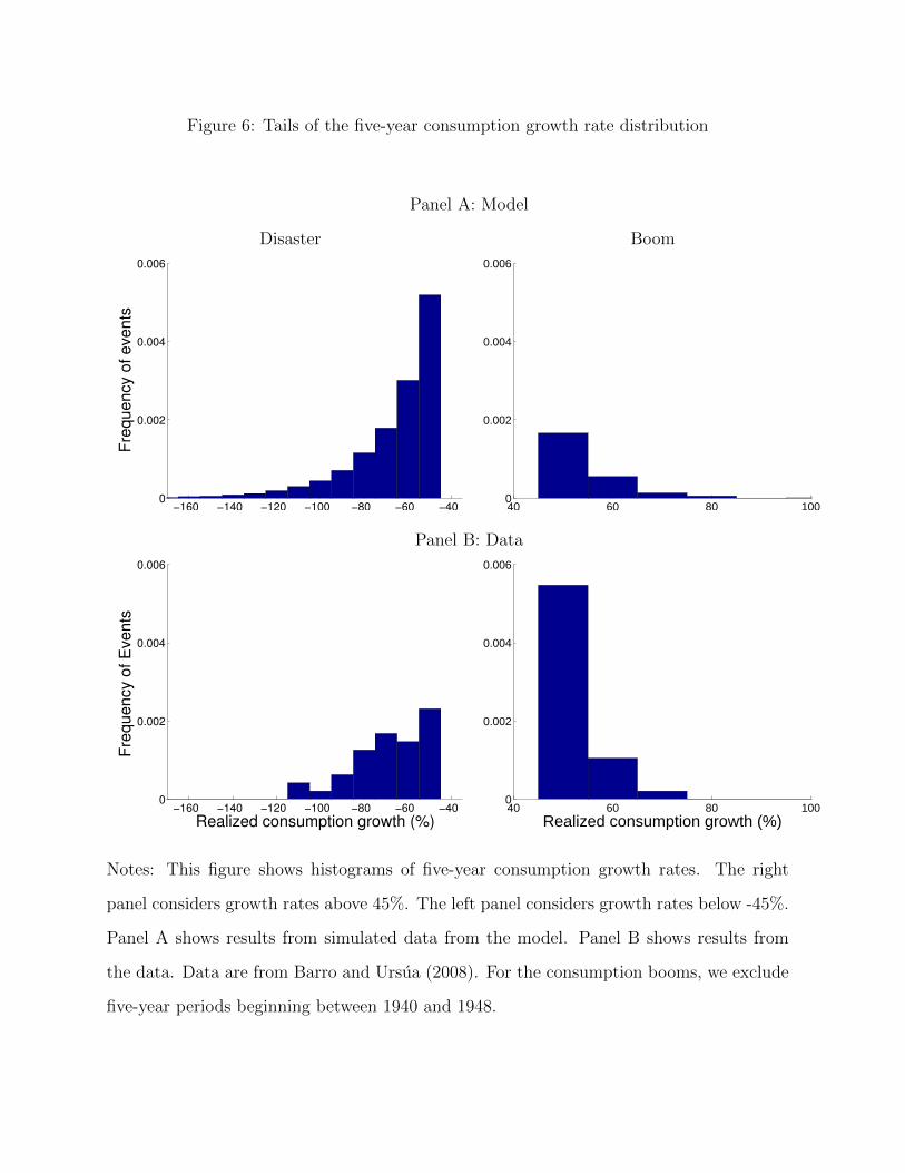
Figure 6: Tails of the five-year consumption growth rate distribution
Panel A: Model
Disaster Boom
−160 −140 −120 −100 −80 −60 −400
0.002
0.004
0.006
Fre
quency o
f events
40 60 80 1000
0.002
0.004
0.006
Panel B: Data
−160 −140 −120 −100 −80 −60 −400
0.002
0.004
0.006
Realized consumption growth (%)
Fre
quency o
f E
vents
40 60 80 1000
0.002
0.004
0.006
Realized consumption growth (%)
Notes: This figure shows histograms of five-year consumption growth rates. The right
panel considers growth rates above 45%. The left panel considers growth rates below -45%.
Panel A shows results from simulated data from the model. Panel B shows results from
the data. Data are from Barro and Ursua (2008). For the consumption booms, we exclude
five-year periods beginning between 1940 and 1948.

Figure 7: Sensitivity of the observed value premium to parameter choices
Panel A: Value premium as a function of average boom probability (λ2)
0.01 0.02 0.03 0.04 0.05
0
0.8
1.6
2.4
3.2
E[R
v]−
E[R
g]
(%)
Boom probability (%)
Panel B: Value premium as a function of the power law tail parameter (α)
0 20 40 60 80 100
0
0.8
1.6
2.4
3.2
E[R
v]−
E[R
g]
(%)
Boom power law alpha
Notes: Panel A reports the observed value premium (defined as the average difference be-
tween the return on the value sector and the return on the growth sector across simulations
with no rare events) as a function of the average probability of a boom. All other param-
eters are unchanged. Panel B reports the average value premium across simulations with
no rare events as a function of the power law parameter α. Lower values of α correspond
to thicker tails.

Figure 8: Consumption growth skewness
0 0.02 0.04 0.06 0.08 0.1−6.5
−6
−5.5
−5
−4.5
−4
−3.5
−3
−2.5
−2
−1.5
disaster probability
co
nsu
mp
tio
n g
row
th s
ke
wn
ess
0 0.02 0.04 0.06 0.08 0.1−7.5
−7
−6.5
−6
−5.5
−5
−4.5
−4
−3.5
boom probability
co
nsu
mp
tio
n g
row
th s
ke
wn
ess
Notes: This figure shows the consumption growth skewness conditional on different rare
event probability. The one on the left plots the skewness at different disaster probability
λ1, with the boom probability equals to its mean. The one on the right plots the skewness
at different boom probability λ2, with the disaster probability equals to its mean. We
calculate skewness by simulating 500,000 years of consumption growth at a monthly
frequency for each value of the rare event probabilities. We aggregate the monthly
consumption growth to an annual frequency and calculate the skewness over the sample.
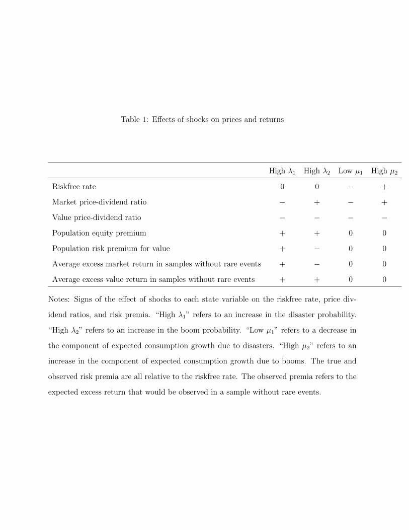
Table 1: Effects of shocks on prices and returns
High λ1 High λ2 Low µ1 High µ2
Riskfree rate 0 0 − +
Market price-dividend ratio − + − +
Value price-dividend ratio − − − −
Population equity premium + + 0 0
Population risk premium for value + − 0 0
Average excess market return in samples without rare events + − 0 0
Average excess value return in samples without rare events + + 0 0
Notes: Signs of the effect of shocks to each state variable on the riskfree rate, price div-
idend ratios, and risk premia. “High λ1” refers to an increase in the disaster probability.
“High λ2” refers to an increase in the boom probability. “Low µ1” refers to a decrease in
the component of expected consumption growth due to disasters. “High µ2” refers to an
increase in the component of expected consumption growth due to booms. The true and
observed risk premia are all relative to the riskfree rate. The observed premia refers to the
expected excess return that would be observed in a sample without rare events.
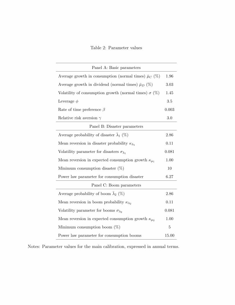
Table 2: Parameter values
Panel A: Basic parameters
Average growth in consumption (normal times) µC (%) 1.96
Average growth in dividend (normal times) µD (%) 3.03
Volatility of consumption growth (normal times) σ (%) 1.45
Leverage φ 3.5
Rate of time preference β 0.003
Relative risk aversion γ 3.0
Panel B: Disaster parameters
Average probability of disaster λ1 (%) 2.86
Mean reversion in disaster probability κλ1 0.11
Volatility parameter for disasters σλ1 0.081
Mean reversion in expected consumption growth κµ1 1.00
Minimum consumption disaster (%) 10
Power law parameter for consumption disaster 6.27
Panel C: Boom parameters
Average probability of boom λ2 (%) 2.86
Mean reversion in boom probability κλ2 0.11
Volatility parameter for booms σλ2 0.081
Mean reversion in expected consumption growth κµ2 1.00
Minimum consumption boom (%) 5
Power law parameter for consumption booms 15.00
Notes: Parameter values for the main calibration, expressed in annual terms.

Table 3: Log consumption and dividend growth moments
Panel A: Consumption growth
No-Jump Simulations All Simulations
Data 0.05 0.50 0.95 0.05 0.50 0.95 Population
mean 1.95 1.65 1.95 2.26 −0.31 1.65 2.70 1.50
standard deviation 1.45 1.22 1.44 1.66 1.47 3.16 7.52 4.24
skewness −0.37 −0.50 0.00 0.48 −4.56 −1.63 2.21 −4.80
kurtosis 3.22 2.20 2.80 3.87 2.85 10.33 28.09 55.34
Panel B: Dividend growth
No-Jump Simulations All Simulations
Data 0.05 0.50 0.95 0.05 0.50 0.95 Population
mean 1.67 1.84 2.91 3.98 −5.01 1.86 5.52 1.31
standard deviation 6.46 4.28 5.04 5.82 5.15 11.05 26.33 14.84
skewness 0.10 −0.50 0.00 0.48 −4.56 −1.63 2.21 −4.80
kurtosis 4.66 2.20 2.80 3.87 2.85 10.33 28.09 55.34
Notes: Data moments are calculated using annual data from 1947 to 2010. Population
moments are calculated from simulating data from the model at a monthly frequency for
600,000 years and then aggregating monthly growth rates to an annual frequency. We also
simulate 100,000 60-year samples and report the 5th-, 50th- and 95th-percentile for each
statistic both from the full set of simulations and for the subset of samples for which no
rare events occur.

Table 4: Value spread moments
No-Jump Simulations All Simulations
Data 0.05 0.50 0.95 0.05 0.50 0.95 Population
exp(E[log(value spread)]) 1.23 1.18 1.21 1.27 1.18 1.23 1.34 1.24
σ(log(value spread)) 0.08 0.02 0.04 0.07 0.03 0.07 0.16 0.10
Value spread autocorrelation 0.79 0.57 0.78 0.90 0.39 0.69 0.89 0.71
Notes: Data moments are calculated using annual data from 1947 to 2010. Population
moments are calculated from simulating monthly data from the model for 600,000 years
and then aggregating to an annual frequency. We also simulate 100,000 60-year samples
and report the 5th-, 50th- and 95th-percentile for each statistic both from the full set of
simulations and for the subset of samples for which no rare events occur. The value spread
is defined as the log of the book-to-market ratio for the value sector minus the book-to-
market ratio for the aggregate market in the data, and as log price-dividend ratio for the
aggregate market minus the log price-dividend ratio for the value sector in the model. In
the data, the growth portfolio is the lowest book-to-market decile. The remaining nine
deciles comprise the value portfolio.

Table 5: Aggregate market moments
No-Jump Simulations All Simulations
Data 0.05 0.50 0.95 0.05 0.50 0.95 Population
E[Rb] 1.25 1.65 1.95 2.10 -0.12 1.62 2.57 1.49
σ(Rb) 2.75 0.13 0.25 0.50 0.38 2.43 5.76 3.24
E[Rm −Rb] 7.25 3.66 5.44 7.94 2.88 5.97 10.28 6.27
σ(Rm) 17.8 10.4 14.5 20.1 13.1 20.5 31.9 22.3
Sharpe ratio 0.41 0.27 0.38 0.51 0.14 0.30 0.46 0.28
exp(E[p− d]) 32.5 25.0 30.7 34.4 20.0 28.6 34.3 27.8
σ(p− d) 0.43 0.10 0.19 0.34 0.14 0.27 0.50 0.35
AR1(p− d) 0.92 0.57 0.78 0.91 0.53 0.78 0.91 0.85
Notes: Data moments are calculated using annual data from 1947 to 2010. Population
moments are calculated from simulating monthly data from the model for 600,000 years
and then aggregating to an annual frequency. We also simulate 100,000 60-year samples
and report the 5th-, 50th- and 95th-percentile for each statistic both from the full set of
simulations and for the subset of samples for which no rare events occur. Rb denotes the
government bond return, Rm denotes the return on the aggregate market and p−d denotes
the log price-dividend ratio.

Table 6: Cross-sectional moments
No-Jump Simulations All Simulations
Data 0.05 0.50 0.95 0.05 0.50 0.95 Population
E[Rv −Rb] 7.95 4.34 6.06 8.52 2.59 5.26 8.28 5.34
E[Rg −Rb] 6.62 1.04 3.37 6.41 1.10 7.90 24.79 9.97
E[Rv −Rg] 1.34 1.26 2.74 4.03 -19.55 -2.42 3.46 -4.63
σ(Rv) 17.0 9.7 13.5 18.7 11.3 17.4 25.2 18.1
σ(Rg) 21.0 16.6 22.8 32.6 21.8 41.8 117.3 64.0
σ(Rv −Rg) 11.7 10.7 14.6 19.9 13.1 35.1 116.1 60.7
Sharpe ratio, value 0.48 0.34 0.45 0.60 0.13 0.31 0.51 0.29
Sharpe ratio, growth 0.32 0.05 0.15 0.24 0.04 0.18 0.29 0.16
Sharpe ratio, value-growth 0.11 0.07 0.19 0.33 -0.20 -0.07 0.25 -0.08
alpha, value 1.26 0.79 1.08 1.50 -0.22 0.86 2.82 1.23
alpha, growth -1.26 -5.96 -4.32 -3.10 -9.62 -3.17 1.36 -4.28
alpha, value-growth 2.53 3.97 5.41 7.33 -1.53 4.07 12.29 5.51
beta, value 0.92 0.86 0.92 0.96 0.26 0.83 0.96 0.66
beta, growth 1.09 1.21 1.41 1.63 1.23 1.69 3.64 2.27
beta, value-growth -0.16 -0.75 -0.49 -0.25 -3.32 -0.87 -0.28 -1.62
Notes: Data moments are calculated using annual data from 1947 to 2010. Population
moments are calculated from simulating monthly data from the model for 600,000 years
and then aggregating to an annual frequency. We also simulate 100,000 60-year samples
and report the 5th-, 50th- and 95th-percentile for each statistic both from the full set of
simulations and for the subset of samples for which no rare events occur. Rv denotes the
gross return on the value sector, Rg denotes the gross return on the growth sector, alpha
denotes the loading of the constant term of the CAPM regression and beta denotes the
loading on the market equity excess return of the CAPM regression. In the data, the
growth portfolio is the lowest book-to-market decile. The remaining nine deciles comprise
the value portfolio.

Table 7: Long-horizon regressions of aggregate market and value-minus-growth returns on
the price-dividend ratio and the value spread
1-year Horizon 3-year Horizon 5-year Horizon
Data NJ All Pop. Data NJ All Pop. Data NJ All Pop.
Panel A: Market returns on the price-dividend ratio
Coef. −0.12 −0.28 −0.17 −0.09 −0.29 −0.67 −0.42 −0.23 −0.41 −0.91 −0.60 −0.35
t-stat [−2.41] [−3.37] [−3.37]
R2 0.09 0.15 0.07 0.02 0.22 0.33 0.16 0.05 0.27 0.43 0.22 0.07
Panel B: Market returns on the value spread
Coef. −0.50 −0.76 −0.33 −0.06 −1.18 −1.88 −0.86 −0.17 −1.28 −2.61 −1.26 −0.25
t-stat [−1.86] [−2.28] [−3.13]
R2 0.05 0.05 0.02 0.001 0.12 0.12 0.06 0.002 0.09 0.16 0.08 0.003
Panel C: Value-minus-growth returns on the price-dividend ratio
Coef. 0.01 0.11 0.06 0.01 0.05 0.27 0.16 0.02 0.09 0.38 0.24 0.02
t-stat [0.37] [0.51] [0.76]
R2 0.00 0.03 0.02 1×10⁻⁴ 0.01 0.07 0.05 2×10⁻⁴ 0.02 0.10 0.07 2×10⁻⁴
Panel D: Value-minus-growth returns on the value spread
Coef. 0.46 1.18 0.47 0.01 1.13 2.87 1.23 0.03 1.48 3.95 1.81 0.05
t-stat [2.52] [2.44] [2.37]
R2 0.10 0.10 0.03 1×10⁻⁵ 0.19 0.25 0.08 5×10⁻⁵ 0.21 0.34 0.12 7×10⁻⁵
Notes: Coefficients and R2-statistics from predictive regressions in annual (overlapping) postwar
data and in the model. In Panels A and B the excess market return is regressed against the
price-dividend ratio and the value spread respectively. Panels C and D repeat this exercise with
the value-minus-growth return. The value spread is defined as the log book-to-market ratio of the
value sector minus log book-to-market ratio of the aggregate market. For the data coefficients, we
report t-statistics constructed using Newey-West standard errors. Population moments (Pop.) are
calculated from simulating monthly data from the model for 600,000 years and then aggregating
to an annual frequency. We also simulate 100,000 60-year samples and report the average value
for each statistic both from the full set of simulations (All) and for the subset of samples for which
no rare events occur (NJ).

Table 8: Data on portfolios formed on the book-to-market ratio
All stocks Top size quintile
G V G V
1 2 3 4 5 1 2 3 4 5
Panel A: 1947 – 2010
E[Ri −Rf ] 6.08 6.71 8.04 8.61 10.36 6.22 6.46 7.26 7.32 8.36
se (0.59) (0.55) (0.52) (0.54) (0.62) (0.57) (0.54) (0.52) (0.55) (0.62)
σ[Ri −Rf ] 16.26 15.12 14.47 14.96 17.20 15.85 14.94 14.48 15.16 17.32
βi 1.06 1.02 0.95 0.96 1.05 1.02 0.99 0.91 0.93 0.99
se (0.02) (0.01) (0.02) (0.02) (0.03) (0.02) (0.01) (0.02) (0.02) (0.03)
% of total market 40.84 22.24 17.03 12.22 7.66 33.85 16.86 12.37 8.01 4.33
Panel B: 1995 – 2000
E[Ri −Rf ] 16.15 15.07 14.63 15.50 13.00 17.84 16.13 14.80 16.09 12.03
se (2.04) (1.82) (1.77) (1.60) (1.40) (2.01) (1.88) (1.93) (1.91) (1.73)
σ[Ri −Rf ] 17.27 15.41 15.03 13.60 11.88 17.04 15.98 16.36 16.18 14.68
βi 1.09 1.10 1.04 0.89 0.78 1.09 1.12 1.10 0.95 0.85
se (0.08) (0.04) (0.06) (0.05) (0.04) (0.08) (0.03) (0.06) (0.09) (0.07)
% of total market 47.53 21.66 14.69 9.33 6.80 40.21 16.75 10.31 5.76 3.92
Panel C: 1929 – 1932
E[Ri −Rf ] -21.79 -20.99 -28.65 -21.52 -26.35 -21.48 -19.26 -28.72 -29.79 -16.94
se (5.77) (5.71) (7.14) (8.82) (9.12) (5.77) (5.70) (7.47) (8.79) (8.74)
σ[Ri −Rf ] 39.98 39.58 49.44 61.08 63.21 39.99 39.48 51.79 60.89 60.58
βi 0.95 0.94 1.15 1.38 1.44 0.95 0.93 1.19 1.36 1.23
se (0.04) (0.03) (0.06) (0.13) (0.12) (0.04) (0.03) (0.07) (0.11) (0.17)
% of total market 46.62 24.56 18.22 8.40 2.20 42.72 20.30 14.50 6.01 0.89
Panel D: January 2008 - June 2009
E[Ri −Rf ] -19.57 -26.92 -29.31 -35.29 -23.61 -19.25 -27.88 -32.22 -39.58 -20.84
se (5.69) (5.03) (6.28) (6.64) (7.64) (5.49) (4.59) (6.15) (6.71) (7.23)
σ[Ri −Rf ] 24.13 21.36 26.64 28.17 32.40 23.29 19.49 26.07 28.47 30.66
βi 0.91 0.82 1.01 1.07 1.20 0.87 0.73 0.97 1.06 1.10
se (0.06) (0.03) (0.07) (0.05) (0.12) (0.06) (0.04) (0.09) (0.06) (0.13)
% 37.02 26.05 16.32 13.82 6.79 30.19 20.63 12.17 10.13 3.96
Notes: Statistics for portfolio excess returns formed by sorting stocks by the ratio of book equity to market
equity during various subperiods of the data. The panel reports means and βs with respect to to the
value-weighted CRSP market portfolio. Data are at a monthly frequency. We multiply excess returns by
1200 to obtain annual percent returns. Excess returns are measured relative to the 30-day Tbill. The left
panel reports results from the full set of equities, while the right panel looks only at the top size quintile.

Table 9: Upside and downside betas in the model
E[R−Rb] (%) relative β+ relative β−
Value 6.06 -0.0024 0.0062
Growth 3.37 0.0686 -0.0634
Notes: This table reports the relative upside and downside betas for the value and growth port-
folios in the model, along with the average returns on these portfolios. The first column reports
the average annual excess returns for value and growth, the second row reports the relative upside
betas, β+i − βi, where β+
i = cov(Ri−Rm|Rm>µm)var(Rm|Rm>µm) , µm is the average return on the aggregate market
within each simulation, and βi is the regular CAPM beta for value and growth portfolio. The
third column reports the relative downside betas, β−i − β, where β−i = cov(Ri−Rm|Rm<µm)var(Rm|Rm<µm) . We
simulate 100,000 60-year samples and report the median values from the subset of samples for
which no rare events occur.