Rapidly-Varying Speed of Sound, Scale Invariance

and Non-Gaussian Signatures

Justin Khoury and Federico Piazza

Perimeter Institute for Theoretical PhysicsWaterloo, Ontario, N2L 2Y5, Canada

Abstract

We show that curvature perturbations acquire a scale invariant spectrum for any constant

equation of state, provided the fluid has a suitably time-dependent sound speed. In order

for modes to exit the physical horizon, and in order to solve the usual problems of standard

big bang cosmology, we argue that the only allowed possibilities are inflationary (albeit

not necessarily slow-roll) expansion or ekpyrotic contraction. Non-Gaussianities offer many

distinguish features. As usual with a small sound speed, non-Gaussianity can be relatively

large, around current sensitivity levels. For DBI-like lagrangians, the amplitude is negative in

the inflationary branch, and can be either negative or positive in the ekpyrotic branch. Unlike

the power spectrum, the three-point amplitude displays a large tilt that, in the expanding

case, peaks on smallest scales. While the shape is predominantly of the equilateral type in

the inflationary branch, as in DBI inflation, it is of the local form in the ekpyrotic branch.

The tensor spectrum is also generically far from scale invariant. In the contracting case, for

instance, tensors are strongly blue tilted, resulting in an unmeasurably small gravity wave

amplitude on cosmic microwave background scales.

arX

iv:0

811.

3633

v4 [

hep-

th]

17

Mar

201

1

1 Introduction

The observation that the large scale structure originated from a nearly scale invariant primordial

spectrum is generally construed as evidence that the universe underwent a phase of quasi-de Sitter

expansion. Given the limited number of early universe parameters constrained by observations

thus far, however, it is prudent to keep an open mind and seek the most general mechanism for

producing density perturbations consistent with the data. It is well-known that generating a scale

invariant spectrum of curvature perturbations with a single scalar field in 3+1 dimensions requires

either inflation or a contracting dust-dominated phase [1, 2]. On the other hand, scale invariant

entropy perturbations can be generated in a larger variety of cosmological scenarios, provided

more than one scalar field is present. This has been shown to occur, for example, in the slowly

contracting background of the new ekpyrotic cosmology [3, 4, 5, 6, 7, 8] or in the kinetic dominated

pre-big bang cosmology [9, 10]. (See [11] and [12] for recent reviews of the ekpyrotic/cyclic and

pre-big bang scenarios, respectively.) Entropy perturbations can then be converted into curvature

perturbations, for instance if the curvaton mechanism [13, 14, 15] is at work. These earlier studies

all have in common a constant sound speed cs for scalar field fluctuations.

In this paper we show that allowing for a time-dependent sound speed greatly broadens the

range of possible cosmologies. The curvature perturbation on uniform density hypersurfaces ζ

can acquire a scale invariant spectrum for arbitrary background equation of state parameter

ε = −H/H2 = 3(1 + w)/2, as long as the sound speed varies appropriately.

Although our derivation applies to any perfect fluid, we take as our fiducial model a single

scalar field φ with a Lagrangian

Lφ =√−gP (X,φ) (1.1)

which is a general function of the kinetic term X = −12gµν∂µφ∂νφ and the field itself. In this

theory the perturbations around a homogeneous background are still adiabatic. However, the

presence of a non-standard kinetic term allows for a background dependent “speed of sound” of

the fluctuations1

c2s =P,Xρ,X

=P,X

P,X + 2XP,XX, (1.2)

where ρ = 2XP,X−P is the energy density of the field, and the quantities above are calculated on

the unperturbed solution. While our basic mechanism for generating a scale invariant spectrum

only relies on a varying sound speed of the adiabatic perturbations, we will refer more specifically

to the single scalar field model (1.1) for calculating non-Gaussianities.

In terms of the rate of change of the sound speed, εs ≡ cs/csH, exact scale invariance requires

ε, εs to be constant and to satisfy a relation between them. More precisely, we find two branches

of solutions:

1Analogously, higher order curvature terms can induce a sound speed of tensor perturbations [16].

1

• Case I: Expanding universe with decreasing sound speed, such that εs = −2ε.

• Case II: Contracting universe with increasing sound speed, such that εs = 25(3− 2ε).

In the expanding case this mechanism was first proposed by [17] (see also [18, 19]), whereas the

contracting branch of solutions is new. Unlike [18], who considered a universe with superluminal

sound speed initially, here we restrict our analysis to subluminal sound speeds throughout. (The-

ories with superluminal propagation have been argued not have a consistent UV-completion [20].)

In the special case εs = 0, these recover de Sitter expansion and dust-like contraction, respec-

tively. Of course, small deviations from these conditions and/or mild time-dependence for ε,εs lead

to small departures from scale invariance. In order for perturbations to be stretched outside the

Hubble horizon, the equation of state must satisfy ε < 1 in Case I, corresponding to inflationary

expansion, or ε > 1 in Case II, corresponding to decelerated contraction. While the expand-

ing branch requires inflation, it is worth emphasizing that our mechanism is not constrained by

slow-roll conditions and therefore encompasses a much broader range of inflationary cosmologies.

The above cosmologies, while degenerate at the level of the power spectrum, can be dis-

tinguished through their non-Gaussian signatures. To begin with, the sign of the three-point

amplitude is generically negative in Case I and can be either negative or positive in Case II.

More importantly, unlike standard inflationary models, here the near scale invariance of the two-

point function does not extend to the three-point amplitude. The non-Gaussian amplitude is

proportional to 1/c2s evaluated at horizon crossing, and therefore exhibits strong running with

scale [21, 22]. In particular, non-Gaussianity peaks on the smallest scales in Case I since cs de-

creases in time, whereas the opposite is generally true in Case II. The sign of the tilt therefore

allows to distinguish between the expanding and contracting branches.

The shape of the three-point function in momentum space is also characteristically different in

the two branches. In the expanding case, the three-point amplitude peaks for equilateral momen-

tum triangles [23], as usual for models with small sound speed such as Dirac-Born-Infeld (DBI)

inflation [24, 25, 26]. In the contracting case, however, the non-Gaussian signal features a strong

peak for squeezed triangles, corresponding to the so-called local form [27]. This may come as a

surprise since local non-Gaussianities usually require two scalar fields, as in the curvaton [14], mod-

ulated reheating [28], pre-big bang pump field [10] and New Ekpyrotic mechanisms [6, 29, 30, 31].

In fact, the striking difference in shape between Cases I and II traces back to the evolution

of ζ at long wavelengths. In the expanding branch, the growing mode of ζ is a constant, and

non-linearities have therefore a finite time to grow until modes go outside the horizon. Maxi-

mal amplification is achieved when all wavevectors have magnitude comparable to the Hubble

radius, leading to the predominantly equilateral shape. In the contracting branch, on the other

hand, ζ keeps growing on super-Hubble scales, thereby allowing non-linearities to grow well after

modes have exited the horizon. The non-Gaussian amplitude therefore peaks when one of the

2

wavenumbers is small, corresponding to the squeezed-triangle limit.

The behavior of ζ on super-Hubble scales is closely related to the issue of stability of the

background. In the long-wavelength limit, ζ represents a mildly scale-dependent perturbation in

the scale factor [32, 33]. Thus all Case I cosmologies are stable, since a constant ζ can be absorbed

in a spatial diffeomorphism. Meanwhile, the super-Hubble growth of ζ in Case II indicates that

these backgrounds are unstable. Remarkably, such tachyonic instabilities appear to be a ubiquitous

feature of contracting mechanisms: both New Ekpyrotic Cosmology and the general class of

contracting two-field models of [36] display a tachyonic instability in the entropy direction. This

by no means represents a show-stopper — it was shown in [37], for instance, that a pre-ekpyrotic

stabilizing phase can bring the field trajectory arbitrarily close to the desired classical solutions for

a broad range of initial conditions. Moreover, as the present work underscores, the super-horizon

growth of ζ leads to striking features in non-Gaussianity.

Another important observable are primordial gravitational waves. Since tensor modes are

oblivious to the time dependence of the sound speed and only feel the background cosmology,

their spectrum is in general not scale invariant. In the expanding case, the gravity wave amplitude

peaks on large scales, corresponding to a red tensor spectral tilt. In the contracting case, gravity

waves are peaked on small scales, corresponding to a strong blue tilt.

Various phenomenological considerations constrain the allowed equation of state parameter.

We have already mentioned the inflationary condition ε < 1 in Case I, in order for perturbations to

exit the Hubble horizon. However, this range of ε of course also ensures that (moderate amounts

of) spatial curvature and anisotropy become increasingly irrelevant in time. If we impose similar

standards in Case II, we obtain ε > 3 (or w > 1), corresponding to the ekpyrotic range. Indeed,

ekpyrotic contraction is equally powerful as inflation in solving the homogeneity, isotropy and flat-

ness problems of standard big bang cosmology [2, 38]. Furthermore, the tilt of non-Gaussianities

cannot be too strong, for otherwise perturbations risk exiting the perturbative regime within the

observable range (Case I) or lead to an unacceptably large amplitude on cosmic microwave back-

ground (CMB) scales (Case II). These non-Gaussian considerations lead to ε . 0.5 in Case I. In

Case II, on the other hand, non-Gaussianities are generically much larger and constrain the model

in the region of the cs − ε parameter space plotted in Fig. 2. Finally, since the tensor spectrum is

red in the expanding case, we must ensure that the gravitational wave amplitude on large scales

is consistent with CMB bounds. This requires the slighly tighter bound: ε . 0.3 (Case I).

While our analysis applies to general scalar field models of the form (1.1), we also provide

explicit microphysical realizations of the scale invariant conditions within the context of DBI

effective lagrangians. Here we piggyback on [39], where it was shown that any scaling solution

for the scale factor and sound speed can be obtained by suitably choosing the warp factor f(φ)

and scalar potential V (φ). Remarkably, the desired condition εs = −2ε is satisfied (at least in

the regime of small sound speed) for the AdS warp factor and m2φ2 potential originally studied

3

by [24]. Thus scale invariance obtains in this case without requiring the slow roll condition ε� 1.

To conclude this introduction, we offer an executive summary of our key results:

• A scale invariant spectrum of perturbations can be obtained for any background cosmology

with constant equation of state, by suitably choosing the time dependence of the sound

speed. We find both an expanding (Case I) and a contracting (Case II) branch of solutions.

We discuss this basic mechanism in Secs. 2 and 3.

• In the expanding case, various phenomenological bounds constrain the equation of state

parameter to ε . 0.3 and are discussed in Sec. 4. Our inflationary range is much broader

than allowed by the usual slow-roll conditions.

• Scale invariance requires ε,εs to be constant and to satisfy a specific relation (see above).

Deviations from these conditions lead to a non-zero spectral tilt, which is derived in Sec. 5.

• Gravitational waves are far from scale invariant. The tensor spectral index, derived in Sec. 6,

is negative in Case I and positive in Case II, corresponding to red and blue tilts, respectively.

• Relatively large non-Gaussianities are generated in both cases (Secs. 7 and 8). In Case I

they are of the DBI-equilateral type and generically negative; in Case II they are of the local

type and generically positive.

• A (nearly) scale invariant two-point function does not necessarily imply a (nearly) scale

invariant three point function. In fact, our mechanism fails to protect against running of

non-Gaussianities. In Case I the three-point function has a strong blue tilt; in Case II it

generally has a strong red tilt (see Sec. 8.2).

2 Scale Invariance from Time-Dependent Sound Speed

Our key observation is that in the presence of a time-dependent sound speed cs the curvature per-

turbation evolves according to an effective cosmological background different from the actual scale

factor. Thus, a scale-invariant spectrum of density perturbations can arise for any background

equation of state parameter ε = −H/H2, for a suitably-varying cs. In this Section, we show that

scale invariance can also obtain in the contracting case as well.

At quadratic order, the action for the curvature perturbation ζ for general speed of sound

models is given by [40]

S =M2

Pl

2

∫d3xdτ z2

[(dζ

dτ

)2

− c2s(~∇ζ)2

], (2.1)

4

where τ is conformal time, and z is defined as usual by z = a√

2ε/cs. This holds whether the

matter is a perfect fluid or a P (X,φ) scalar field. Since cs is a general function of time, it is

convenient to instead work in terms of the “sound-horizon” time dy = csdτ :

S =M2

Pl

2

∫d3xdy q2

[ζ ′2 − (~∇ζ)2

], (2.2)

where ′ ≡ d/dy, and

q ≡√csz =

a√

2ε√cs

. (2.3)

The virtue of this time redefinition is manifest: the kinetic term takes the standard form, as if

cs = 1, while the dependence on cs has been absorbed in a modified background described by q.

In terms of the canonically-normalized scalar variable v = MPlqζ, the equations of motion for

the Fourier modes are given by

v′′k +

(k2 − q′′

q

)vk = 0 . (2.4)

It is well-known that this results in a scale-invariant spectrum if and only if q′′/q = 2/y2. Indeed,

for the adiabatic vacuum choice, the mode functions are given by

vk(y) =1√2k

(1− i

ky

)e−iky , (2.5)

resulting in a scale-invariant Pv(k) ∼ k3v2k in the limit k → 0. Therefore, there are two possibilities:

q ∼ (−y)−1 or q ∼ y2 , (2.6)

where y runs from −∞ to 0. In the limit of constant cs, these of course reduce to de Sitter

expansion and dust-dominated contraction [1, 2], respectively. But, as we now show, more general

backgrounds can also do the trick for suitably-chosen cs.

To proceed, let us assume for simplicity that the background has constant equation of state:

ε = const. Similarly, as usual we can define a rate of change parameter εs for the sound speed,

εs =csHcs

, (2.7)

also assumed to be constant. (In Sec. 5, we will relax these assumptions when calculating the

spectral tilt.) From the definition of y, it is then straightforward to show that

a(y) ∼ (−y)1

εs+ε−1 ; cs(y) ∼ (−y)εs

εs+ε−1 . (2.8)

Substituting these into (2.3), then from (2.6) we deduce that scale-invariance occurs either for

εs = −2ε (Case I) , (2.9)

5

corresponding to an expanding background with decreasing sound speed, or

εs =2

5(3− 2ε) (Case II) , (2.10)

corresponding to a contracting universe with growing sound speed (for ε > 3/2). Case I was pointed

out in [17, 18, 19] (see also [39] for a realization in DBI models of inflation [24]), whereas Case II

is new. As a check, with εs = 0 this recovers de Sitter expansion (ε = 0) or dust-like contraction

(ε = 3/2). In slow-roll inflation, ε is by definition small, and scale invariance forces εs to be small

as well. What the above results show, however, is that much larger values of ε are allowed as well,

provided εs is chosen appropriately.

3 Amplitude of Perturbations and Stability

From the explicit solution for vk in (2.5), we can read off the long-wavelength amplitude for

ζk = vk/q:

k3/2 |ζk| =√cs

2MPl

√εay

. (3.1)

This can be further simpified by noting that (2.8) allows to solve for y in terms H, a and cs.

Substituting the result into the above amplitude, the ζ power spectrum is readily obtained:

Pζ ≡1

2π2k3 |ζk|2 =

1

8π2ε(εs + ε− 1)2

H2

csM2Pl

. (3.2)

In the quasi-de Sitter and nearly constant cs limit, ε � 1 and εs � 1, this agrees with earlier

results [40].

Although the above expression for Pζ applies both to Cases I and II, the time-dependence

of the right-hand side is different in each case. In Case I, H2/cs is constant — see (2.8) —,

and, following standard conventions, it therefore makes sense to evaluate Pζ at horizon-crossing

(denoted by “bars”):

P(I)ζ =

(1 + ε)2

8π2ε

H2

csM2Pl

, (3.3)

where we have substituted (2.9).

In Case II, on the other hand, H2/cs ∼ 1/y6, and the amplitude for ζ keeps growing outside

the horizon. Moreover, unlike Case I, here the final amplitude depends not only on the dynamics

during the scale invariant phase, but also on the details of whatever phase precedes the bounce.

For definiteness, we will assume that super-horizon modes stop growing after the scale invariant

phase. This is achieved, for instance, if cs saturates to a constant value and the collapse carries on

6

with an equation of state w > 1, or ε > 3. In this case, the final amplitude of the power spectrum

is evaluated at the end of the scale-invariant phase:

P(II)ζ =

(1 + ε)2

200π2ε

H2end

cs endM2Pl

, (3.4)

where now we have substituted (2.10).

Of course this difference in time-dependence is intimately tied to the stability of the back-

ground. In the infinite-wavelength or k → 0 limit, classical solutions for ζ are interpreted as

homogeneous perturbations to the background scale factor [32, 33]:

ds2 = a2(τ)(−dτ 2 + e2ζd~x2) . (3.5)

From ζ = v/q and the explicit solution (2.5), we see that the growing mode is ζ ∼ 1/qy. In Case I,

which includes standard inflation, q ∼ 1/y, and ζ → const. on super-Hubble scales [34, 35]. Thus

these backgrounds are stable. In Case II, however, q ∼ y2, and the growth of ζ as k → 0 indicates

that the background is not an attractor.

This instability appears to be a ubiquitous feature of all contracting mechanisms for generating

perturbations. In the two-field ekpyrotic mechanism, for instance, the entropy direction must be

tachyonic [3, 7, 37]. This was shown to be true for arbitrary two-derivative action of two scalar

fields with general contracting backgrounds [36]. And here we find that these conclusions also

apply to our single-field mechanism.

Nevertheless, this instability should not be construed as a show-stopper. In the New Ekpyrotic

scenario, for instance, it is circumvented by including a pre-ekpyrotic stabilizing phase that brings

the field arbitrary close to the tachyonic ridge [37]. More importantly, as we will see later on, the

growth of ζ on super-Hubble scales enhances non-linearities and leads to interesting non-Gaussian

signatures.

4 Phenomenological Considerations

In this Section we describe various constraints on the scale invariant phase, ranging from requiring

that the modes, generated inside the sound horizon, cross the Hubble horizon, to solving the

standard problems of big bang cosmology, to generating acceptable levels of non-Gaussianity. We

will see that these conditions together require the background evolution to be inflationary (in the

expanding case) or ekpyrotic (in the contracting case).

4.1 Generating super-Hubble modes

For general ε, the amplification and freeze-out mechanism described above relies on a rapidly

changing sound horizon. And indeed it is conceivable that the Hubble radius and sound horizons

7

are vastly different during this early-universe phase. But once the universe exits this phase and

becomes radiation dominated, we must ensure that we are left with scale-invariant perturbations

beyond the Hubble radius at reheating. In other words, during the generation of perturbations,

modes must not only exit the sound horizon, but also the Hubble radius.

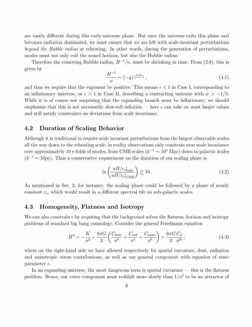
Therefore the comoving Hubble radius, H−1/a, must be shrinking in time. From (2.8), this is

given byH−1

a∼ (−y)

ε−1εs+ε−1 , (4.1)

and thus we require that the exponent be positive. This means ε < 1 in Case I, corresponding to

an inflationary universe, or ε > 1 in Case II, describing a contracting universe with w > −1/3.

While it is of course not surprising that the expanding branch must be inflationary, we should

emphasize that this is not necessarily slow-roll inflation — here ε can take on must larger values

and still satisfy constraints on deviations from scale invariance.

4.2 Duration of Scaling Behavior

Although it is traditional to require scale invariant perturbations from the largest observable scales

all the way down to the reheating scale, in reality observations only constrain near scale invariance

over approximately 10 e-folds of modes, from CMB scales (k−1 ∼ 103 Mpc) down to galactic scales

(k−1 ∼ Mpc). Thus a conservative requirement on the duration of our scaling phase is

ln

(aH/cs|endaH/cs|CMB

)& 10 . (4.2)

As mentioned in Sec. 3, for instance, the scaling phase could be followed by a phase of nearly

constant cs, which would result in a different spectral tilt on sub-galactic scales.

4.3 Homogeneity, Flatness and Isotropy

We can also constrain ε by requiring that the background solves the flatness, horizon and isotropy

problems of standard big bang cosmology. Consider the general Friedmann equation

H2 = −Ka2

+8πG

3

(Cdust

a3+Crad

a4+Caniso

a6

)+

8πG

3

Cφa2ε

, (4.3)

where on the right-hand side we have allowed respectively for spatial curvature, dust, radiation

and anisotropic stress contributions, as well as our general component with equation of state

parameter ε.

In an expanding universe, the most dangerous term is spatial curvature — this is the flatness

problem. Hence, our extra component must redshift more slowly than 1/a2 to be an attractor of

8

the cosmological evolution. By inspection, this requires ε < 1, or w < −1/3, which is again the

condition for inflation.

In a contracting background, on the other hand, the worrisome component is the anisotropy,

which blueshifts as 1/a6. Thus a contracting universe typically becomes increasingly anisotropic,

which is at the root of chaotic mixmaster behavior [41, 42]. In order to blueshift faster and

win over anisotropy, our component must satisfy ε > 3, or w > 1 [2, 38]. This is the ekpyrotic

branch [3, 43, 44, 45, 46, 47]. See [11] for a review of the ekpyrotic/cyclic scenario. Indeed,

ekpyrotic contraction does equally well at solving the flatness, horizon and isotropy problems as

inflationary expansion does.

Two points are worth emphasizing:

• The model with varying sound speed described here is the first example of a single-field

ekpyrotic model resulting in an unambiguously scale invariant spectrum for the curvature

perturbation. The earliest renditions of the ekpyrotic/cyclic scenarios also invoked a single

scalar field, but ζ was not scale invariant during the contracting phase, and one had to invoke

higher-dimensional effects at the singularity [46, 48, 49, 50] or a breakdown of the equation

of motion for ζ at the bounce [51]. In New Ekpyrotic Cosmology, this issue was resolved by

using two ekpyrotic scalar fields to generate a scale-invariant entropy perturbation [3, 4, 5,

6, 7, 8].

• These earlier mechanisms, either relying on matching conditions at the singularity or with

two scalar fields, all require ε � 3 for the spectrum to be nearly scale invariant. Here the

condition that ε > 3 is much weaker, thereby extending the range of allowed models.

While the range ε > 3 is certainly desirable as it allows the ekpyrotic component to dominate

over all other forms of energy density, this condition is by no means necessary from the strict

point of view of generating perturbations. The actual lower bound comes from generating super-

Hubble modes which, as we have seen in Sec. 4.1, only requires ε > 1. For instance, the instability

in Case II presumably requires some earlier phase to bring the field trajectory sufficiently close

to the desired classical trajectory; this pre-scaling phase could also drive the universe towards

homogeneity and isotropy using the ekpyrotic smoothing mechanism if ε > 3.

4.4 Constraints from Gravity Waves and non-Gaussianities

Further constraints to our model come from the tilt of the gravitational wave spectrum and non-

Gaussianity, which will be discussed in more detail in Secs. 6 and 8.2, respectively. Interestingly,

the cancelation between ε and εs that results in a scale invariant two-point function does not

protect the tensor spectrum nor the three-point function from running.

9

The inflationary branch (Case I) is characterized by a decreasing sound speed, which in turn

leads to larger non-Gaussianities on small scales. In order to maintain perturbative control over

the entire range of modes, we must require ε . 0.5 (or w . −2/3). Meanwhile, the tensor spectrum

is red and therefore peaks on large scales. To satisfy current bounds on the gravitational wave

contribution to the CMB temperature anisotropy, we must impose ε . 0.3.

In the ekpyrotic branch (Case II), the growing sound speed results in non-Gaussianities that

grow in amplitude as we probe larger scales; but clearly the sound speed should not exceed the

speed of light during the evolution. Moreover, the growing of the modes outside the horizon

generate a new plethora of terms that have to be included in the three-point function (see (7.39))

and that can very easily produce unacceptably large level of non-Gaussianity on CMB scales.

However, we can still find a safe region in the (cc,end, ε) parameter space. With fX = 1 — see (7.33)

for its definition—, for instance, the allowed region lies between cs & 0.7 and 2.8 . ε . 3.15, as

shown in Fig. 2. Meanwhile, the tensor spectrum has a strong blue tilt and therefore does not

yield any constraint on the equation of state parameter.

To summarize, for our two branches of solutions, corresponding respectively to expansion and

contraction, we have the allowed respective range for the equation of state parameter:

0 < ε . 0.3 (Case I)

2.8 . ε . 3.15 (Case II) . (4.4)

Intriguingly, the bounds on the equation of state are comparably constraining in each case: roughly

up to 20% allowed deviations from exact de Sitter (−1 < w . −0.8) or kinetic domination

(0.9 < w . 1.1), respectively. Note that in Case II the sound speed must be suitably adjusted

as a function of ε in order to give acceptable non-Gaussianity, as shown in Fig. 2. Each branch

addresses the standard problems of big bang cosmology and, for suitably varying speed of sound,

yields a scale invariant spectrum of density perturbations while being consistent with present

limits on gravitational waves and non-Gaussianity.

5 Scalar Spectral Index

In this Section we consider small departures from exact scale invariance, which occur whenever εsdeviates from the conditions (2.9) or (2.10), and/or when ε, εs are time-dependent. To parametrize

this time dependence, we introduce

η =1

H

d ln ε

dt; ηs =

1

H

d ln εsdt

. (5.1)

For simplicity, we treat η and ηs as small and constant. Nothing else is assumed about ε and εsfor the moment.

10

In this approximation, our time redefinition, dy = csdτ , can be integrated explicitly:

y =cs

(ε+ εs − 1)aH

(1 +

εη + εsηs(ε+ εs − 1)2

). (5.2)

And this in turn can be used to obtain an explicit expression for q′′/q in the mode equation (2.4).

For instance, we have

d ln q

d ln y=

1 + (η − εs)/2ε+ εs − 1

(1 +

εη + εsηs(ε+ εs − 1)2

). (5.3)

Proceeding along these lines, after some straightforward algebra the mode equation takes the form

y2v′′k + y2k2vk −(ν2 − 1

4

)vk = 0 , (5.4)

where

ν2 − 1

4=

1

(ε+ εs − 1)2

{(1 +

η − εs2

)2

− εsηs2

+(1− εs/2)(4− 3εs − 2ε)(εη + εsηs)

(ε+ εs − 1)2

}

− 1 + (η − εs)/2ε+ εs − 1

. (5.5)

As usual we can turn (5.4) into a Bessel equation for vk/√−ky, which, assuming adiabatic

initial conditions, has a Hankel function solution, H(1)ν (−ky). In the long-wavelength limit, the

corresponding spectral index is then

ns − 1 = −2ν + 3 . (5.6)

Thus the spectrum is nearly scale invariant for ν ≈ 3/2. In particular, setting η = ηs = 0, one can

quickly check that exact scale invariance (ν = 3/2) requires that either (2.9) or (2.10) be satisfied.

We next derive explicit expressions for ns for small departures from these conditions.

• Case I: εs ≈ −2ε

It is convenient to characterize deviations from εs = −2ε through a small parameter δI:

εs = −2ε+ (1 + ε)δI . (5.7)

By expanding ν to linear order in δI, η, and ηs, the scalar spectral index is thus given by

(ns − 1)I = −δI −1

(1 + ε)2

[(1 +

11

3ε

)η − 14

3εηs

]. (5.8)

11

As a check, note that in the limit of quasi-de Sitter background and nearly constant cs, for

which ε, εs � 1, we have δI ≈ εs + 2ε, and thus

(ns − 1)slow−roll ≈ −2ε− εs − η . (5.9)

This agrees with earlier treatments [40].

More generally, however, larger values of ε and εs are possible without spoiling approximate

scale invariance, provided δI remains small. Thus the δI parametrization offers a more general

characterization of deviations from ns = 1, which, in the special case ε, εs � 1, reproduces

standard slow-roll results.

Instead of ηs, we can alternatively introduce a parameter δ′I obtained by taking the derivative

of (5.7):

δ′I ≡dδI

d log a. (5.10)

Expressed in terms of this parameter, we find

(ns − 1)I = −δI −1− ε

(1 + ε)2η − 7

3

δ′I1 + ε

. (5.11)

• Case II: εs ≈ 25(3− 2ε)

Similarly, in the contracting branch we can introduce δII as

εs =2

5(3− 2ε)− 1

5(1 + ε)δII . (5.12)

Substituting into (5.5) and, as before, keeping terms linear in δII, η, and ηs, we obtain

(ns − 1)II = −5 δII −5

(1 + ε)2

[(1 +

43

3ε

)η + 70

(1− 2

3ε

)ηs

]. (5.13)

Or, equivalently, in terms of δ′II ≡ dδII/d log a,

(ns − 1)II = −5 δII −5

(1 + ε)2

[(1− 97

3ε

)η − 35

3(1 + ε)δ′II

]. (5.14)

In slow-roll inflation ε and η are usually considered as independent and comparably small

parameters. Similarly, here we treat δ, η and ηs (or δ, η and δ′) on the same footing because

that all appear at linear order in the expression of the observationally small quantity ns − 1. Of

course, more fine tuned cancellations and richer hierarchies between the parameters can also be

considered.

12

6 Gravitational Wave Spectrum

Unlike scalar perturbations, tensor modes are oblivious to a time-dependent sound speed and

instead feel only the cosmological background. The mode functions hk(τ) therefore satisfy

d2hkdτ 2

+

(k2 − 2− ε

(1− ε)2τ 2

)hk = 0 . (6.1)

As usual, this can be cast as a Bessel equation through the field redefinition: uk = ahk/√−kτ .

Assuming adiabatic initial conditions, the solutions are given by

hk(τ) =

√−τπ2a

H(1)12 | 3−ε1−ε |

(−kτ) . (6.2)

• Case I: εs ≈ −2ε

In the inflationary branch, the equation of state parameter falls in the range 0 < ε < 1. The

tensor power spectrum, Ph = k3|hk|2/π2, therefore takes the form

P(I)h ∼

H2end

M2Pl

(k

Hend

)− 2ε1−ε

, (6.3)

corresponding to a red tensor tilt:

n(I)T =

d lnPh(k)

d ln k= − 2ε

1− ε. (6.4)

The tensor-to-scalar ratio follows by comparing with (3.3). Noting that the sound speed

evaluated at horizon crossing satisfies cs ∼ k−2ε/(1+ε), we obtain

r(I) ∼ εcs

(Kend

K

) 4ε2

1−ε2

. (6.5)

And since this amplitude peaks on the largest scales, we have to ensure that this satisfies

current bounds on the gravitational wave contribution to the CMB: rCMB . 0.3. We will

see in Sec. 8 that the non-Gaussian amplitude is proportional to c−2s , and thus the current

constraint from non-Gaussianity gives cs|CMB ∼> 0.1. Moreover, as discussed in Sec. 4.2, we

have Kend/K|CMB ∼> 103. Assuming the minimum required number of e-folds, we obtain the

conservative bound

ε . 0.3 . (6.6)

This confirms the bound quoted in (4.4).

13

• Case II: εs ≈ 25(3− 2ε)

In the ekpyrotic branch, the gravitational wave power spectrum is

P(II)h ∼ H2

end

M2Pl

(k

Hend

)3−| ε−3ε−1|

, (6.7)

For ε > 3 the tensor spectrum has a strong blue tilt:

n(II)T =

2ε

ε− 1> 2 . (6.8)

In particular, the gravitational wave amplitude is negligible on CMB scales in this case, as

in the pre-big bang [9, 52] and ekpyrotic scenarios [43, 53]. For ε < 3 we have

n(II)T =

4ε− 6

ε− 1. (6.9)

The gravitational wave spectrum is flat for ε = 3/2, i.e., in the case of dust-like contrac-

tion [1].

7 Calculating Non-Gaussianities

We now calculate the three-point function for the following general single scalar field model [26, 55]:

S =

∫d4x√−g[R

2+ P (X,φ)

], (7.1)

where the pressure P is a general function of the scalar field φ and the kinetic term X =

−12gµν∂µφ∂νφ. To simplify the expressions below, we set MPl = 1 throughout the calculation.

The energy density reads

ρ = 2XP,X − P , (7.2)

while the speed of sound is given by

c2s =P,Xρ,X

=P,X

P,X + 2XP,XX. (7.3)

Besides the parameters ε, εs, η, ηs introduced earlier, the calculation of the three-point function

also necessitates defining two further parameters derived from P (X,φ) [55, 26]

Σ = XP,X + 2X2P,XX =H2ε

c2s, (7.4)

λ = X2P,XX +2

3X3P,XXX . (7.5)

14

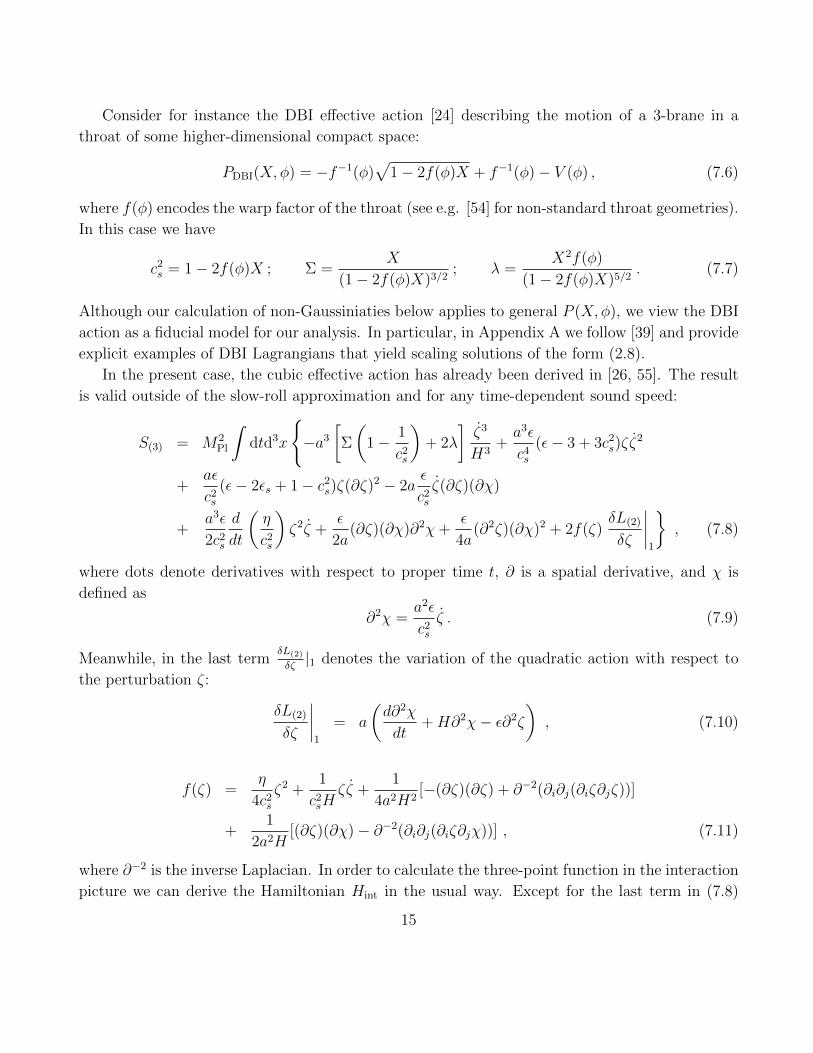
Consider for instance the DBI effective action [24] describing the motion of a 3-brane in a

throat of some higher-dimensional compact space:

PDBI(X,φ) = −f−1(φ)√

1− 2f(φ)X + f−1(φ)− V (φ) , (7.6)

where f(φ) encodes the warp factor of the throat (see e.g. [54] for non-standard throat geometries).

In this case we have

c2s = 1− 2f(φ)X ; Σ =X

(1− 2f(φ)X)3/2; λ =

X2f(φ)

(1− 2f(φ)X)5/2. (7.7)

Although our calculation of non-Gaussiniaties below applies to general P (X,φ), we view the DBI

action as a fiducial model for our analysis. In particular, in Appendix A we follow [39] and provide

explicit examples of DBI Lagrangians that yield scaling solutions of the form (2.8).

In the present case, the cubic effective action has already been derived in [26, 55]. The result

is valid outside of the slow-roll approximation and for any time-dependent sound speed:

S(3) = M2Pl

∫dtd3x

{−a3

[Σ

(1− 1

c2s

)+ 2λ

]ζ3

H3+a3ε

c4s(ε− 3 + 3c2s)ζζ

2

+aε

c2s(ε− 2εs + 1− c2s)ζ(∂ζ)2 − 2a

ε

c2sζ(∂ζ)(∂χ)

+a3ε

2c2s

d

dt

(η

c2s

)ζ2ζ +

ε

2a(∂ζ)(∂χ)∂2χ+

ε

4a(∂2ζ)(∂χ)2 + 2f(ζ)

δL(2)

δζ

∣∣∣∣1

}, (7.8)

where dots denote derivatives with respect to proper time t, ∂ is a spatial derivative, and χ is

defined as

∂2χ =a2ε

c2sζ . (7.9)

Meanwhile, in the last termδL(2)

δζ|1 denotes the variation of the quadratic action with respect to

the perturbation ζ:

δL(2)

δζ

∣∣∣∣1

= a

(d∂2χ

dt+H∂2χ− ε∂2ζ

), (7.10)

f(ζ) =η

4c2sζ2 +

1

c2sHζζ +

1

4a2H2[−(∂ζ)(∂ζ) + ∂−2(∂i∂j(∂iζ∂jζ))]

+1

2a2H[(∂ζ)(∂χ)− ∂−2(∂i∂j(∂iζ∂jχ))] , (7.11)

where ∂−2 is the inverse Laplacian. In order to calculate the three-point function in the interaction

picture we can derive the Hamiltonian Hint in the usual way. Except for the last term in (7.8)

15

we have Hint = −L(3), up to interactions that are higher order in the number of fields. The last

term requires more attention because it contains a second time derivative in the field which makes

problematic the definition of the conjugate momentum. However, since δLδζ|1 is proportional to the

linearized equations of motion, it can be absorbed by a field redefinition

ζ → ζn + f(ζn) . (7.12)

Only the first two terms in (7.11) contribute to the three-point correlation function at long

wavelengths since all other terms involve gradients that go to zero outside the horizon. In Case I,

the second term is also negligible since ζ → const. on super Hubble scales. Thus, after the field

redefinition ζ → ζn + η4c2sζ2n, the three-point function can be expressed in this case as

〈ζ(x1)ζ(x2)ζ(x3)〉(I) = 〈ζn(x1)ζn(x2)ζn(x3)〉

+η

2c2s(〈ζn(x1)ζn(x2)〉〈ζn(x1)ζn(x3)〉+ cyclic) +O(ζ6n) . (7.13)

In Case II, on the other hand, the second term can be simplified by noting that ζ ∼ 1/y3 on

super-Hubble scales. To leading order in η,ηs, it follows from (5.2) and the condition for scale

invariance (2.10) that ζn = −(3/5)H(1 + ε)ζn. Thus the desired field redefinition is ζ → ζn +η4c2sζ2n −

3(1+ε)5c2s

ζ2n, in terms of which the three-point amplitude takes the form

〈ζ(x1)ζ(x2)ζ(x3)〉(II) = 〈ζn(x1)ζn(x2)ζn(x3)〉

+

(η

2c2s− 6(1 + ε)

5c2s

)(〈ζn(x1)ζn(x2)〉〈ζn(x1)ζn(x3)〉+ cyclic)

+ O(ζ6n) . (7.14)

7.1 The three-point function: some useful formulae

We now proceed to calculate the three-point function using standard methods [33]. At first order

in perturbation theory and in the interaction picture we have

〈ζ(t,k1)ζ(t,k2)ζ(t,k3)〉 = −i∫ t

t0

dt′〈[ζ(t,k1)ζ(t,k2)ζ(t,k3), Hint(t′)]〉 , (7.15)

where t0 is some sufficiently early time. It proves convenient to work with the sound horizon time

variable y defined in (5.2) (dy = csdt/a) and expand the field ζ in creators and annihilators in the

usual way:

ζ(y,k) = uk(y)a(k) + u∗k(y)a†(−k). (7.16)

Note that with our Fourier conventions commutation relations read [a(k), a†(k′)] = (2π)3δ3(k−k′).The mode functions uk are easily computed in terms of the canonically normalized mode functions

16

v (2.5). Up to an irrelevant phase, we have

uk(y) =1

a

( cs2ε

)1/2vk(y) =

H(1− ε− εs)2√csk3ε

(1 + iky)e−iky. (7.17)

The contribution to the three-point function of each term in (7.8) can be worked out once we

substitute (7.16) and (7.17) in (7.15). After switching to the integration variable y and making

some simplifications, we encounter integrals of the form

C =

∫ yend

−∞+iε

dy

(y

yend

)γ(−iy)neiKy . (7.18)

Only the imaginary part of this integral is relevant for our calculation. In the above expression,

n is an integer, yend < 0 is the value of y at the end of the inflationary or ekpyrotic phase, and

K ≡ k1 +k2 +k3. Hence, for all modes of interest, K|yend| is a small quantity. As discussed in [33],

the above choice of integration contour picks up the appropriate interacting “in-in” vacuum at

|y| → ∞ and takes care of the oscillating behavior of the exponential.

For simplicity, we consider only strictly scale invariant solutions and therefore neglect small

corrections of order δ, η and ηs in our calculations. The exponent γ is thus a constant, parame-

terizing the behavior of either H/c1/2s or H/c

5/2s , depending on the term being considered. More

specifically, in Case I (expanding branch) we have

H

c1/2s

=Hend

c1/2s end

(γ = 0) ,H

c5/2s

=Hend

c5/2s end

(y

yend

)α(γ = α) , (7.19)

where

α ≡ − 4ε

1 + ε. (7.20)

In Case II, instead,

H

c1/2s

=Hend

c1/2s end

(y

yend

)−3(γ = −3) ,

H

c5/2s

=Hend

c5/2s end

(y

yend

)β(γ = β) , (7.21)

where

β ≡ 5ε− 3

ε+ 1. (7.22)

Let us describe the integrals in more detail for Case I. For γ + n > −2 the imaginary part

of (7.18) is convergent as yend → 0. In this case we can approximately extend the upper limit of

integration to 0, which amounts to neglecting terms of higher order in k|yend|. We thus obtain

Im C = −(K|yend|)−γ cosγπ

2Γ(1 + γ + n)K−n−1 . (7.23)

17

When γ + n < −2, however, the integral (7.18) is divergent for yend → 0. To leading order in

k|yend| we find

Im C = Im(−i)n

γ + n+ 1(yn+1

end + iKyn+2end ) . (7.24)

For example,

Im C =(K|yend|)2

K(γ + 2)(n = 0) , Im C = − (K|yend|)2

K2(γ + 2)(n = 1) , (7.25)

and so forth. For the parameter range relevant to Case II the integrals are calculated in Appendix

B.

7.2 Example 1: the ζζ2 contribution

Before writing our full set of results, it is worth outlining as an example the calculation of the

3-point contribution from the ζζ2 term in (7.8). By applying the commutation relations this reads:

〈ζ(k1)ζ(k2)ζ(k3)〉ζζ2 = i(2π)3δ3(k1 + k2 + k3)uk1(yend)uk2(yend)uk3(yend)

×∫ yend

−∞+iε

dycsa

a3ε

c4s(ε− 3 + 3c2s)u

∗k1

(y)du∗k2(y)

dy

du∗k3(y)

dy+ perm.+ c.c. (7.26)

Substituting (7.17), we have

〈ζ(k1)ζ(k2)ζ(k3)〉ζζ2 = i(2π)3δ3(k1 + k2 + k3)H3

end(1− ε− εs)3

43 ε 3/2 c3/2s end

1

Πjk3j

×∫ yend

−∞+iε

dya2ε

c3s(ε− 3 + 3c2s)

H3(1− ε− εs)3

ε 3/2 c3/2s

(1− ik1y)k22k23y

2eiKy + perm.+ c.c. (7.27)

Since we are considering a strictly scale-invariant solution, ε and εs are constant and can be taken

outside of the integral. Now, we can use (5.2) to substitute for a2y2 and find

〈ζ(k1)ζ(k2)ζ(k3)〉ζζ2 = i(2π)3δ3(k1 + k2 + k3)H3

end(1− ε− εs)4

43 ε2 c3/2s end

1

Πjk3j

×∫ yend

−∞+iε

dyH

c5/2s

(ε− 3 + 3c2s)(1− ik1y)k22k23eiKy + perm.+ c.c. (7.28)

In the expanding case (Case I), εs = −2ε, and the background-dependent functions in the

integrand display the two types of time dependence listed in (7.19). Since both of these give

rise to convergent integrals, we can apply (7.23). Moreover, we combine the prefactor (K|yend|)−γwith the appropriate background functions, Hend/c

1/2s end or Hend/c

5/2s end, to express the corresponding

18

quantities at horizon crossing. In other words, Hendc−1/2s end = Hc

−1/2s , Hendc

−5/2s end(K|yend|)−α =

Hc−5/2s where bar quantities are evaluated at horizon crossing. We finally obtain (Case I)

〈ζ(k1)ζ(k2)ζ(k3)〉ζζ2 (I) = (2π)3δ3(k1 + k2 + k3)H4(1 + ε)4

16ε2 c4s

1

Πjk3j

k22k23

K

×{

(ε− 3) cosαπ

2Γ(1 + α)

[1 + (1 + α)

k1K

]+ 3c2s

[1 +

k1K

]}+ sym. (7.29)

Note that the combination cos απ2

Γ(1 + α), which appears ubiquitously in Case I (see below), is

regular in the limit α→ −1: the constraint α & −1 (ε . 0.3) is uniquely dictated by phenomenol-

ogy.

In the contracting case (Case II), εs = 2(3 − 2ε)/5, and the background-dependent functions

in the integrand follow the power-law behaviors given in (7.21). Moreover, since the amplitudes

of the perturbations keep growing outside the horizon, it is convenient to refer to the background

quantities at the end of the ekpyrosis phase as those directly relate to the power spectrum. This

growth of the amplitude complicates the calculation somewhat compared to the expanding case.

Specifically, the time-derivative of the mode function (7.17) in Case II reads

du†

dy=H(1− ε− εs)

2√csk3ε

[k2y − 3

y(1− iky)

]eiKy . (7.30)

Note that only the first term in square brackets appears in Case I. The presence of the extra terms

results in longer expressions for the amplitudes in Case II. The final answer is given in Sec. 7.4.

7.3 Example 2: the ζ3 contribution

As another example of our method, consider the ζ3 term, for which the three-point function reads

〈ζ(k1)ζ(k2)ζ(k3)〉ζ3 = −i(2π)3δ3(k1 + k2 + k3)uk1(yend)uk2(yend)uk3(yend)

×∫ yend

−∞+iε

dyc2sa2

a3

H3[Σ(1− c−2s ) + 2λ]

du∗k1(y)

dy

du∗k2(y)

dy

du∗k3(y)

dy+ perm.+ c.c. (7.31)

Note that the parameter λ can be written as [55]

λ =Σ

6

(2fXc2s

+1

c2s− 1

), (7.32)

where we have introduced

fX =εεs3εX

, (7.33)

19

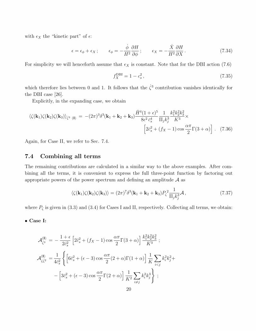
with εX the “kinetic part” of ε:

ε = εφ + εX ; εφ = − φ

H2

∂H

∂φ; εX = − X

H2

∂H

∂X. (7.34)

For simplicity we will henceforth assume that εX is constant. Note that for the DBI action (7.6)

fDBIX = 1− c2s , (7.35)

which therefore lies between 0 and 1. It follows that the ζ3 contribution vanishes identically for

the DBI case [26].

Explicitly, in the expanding case, we obtain

〈ζ(k1)ζ(k2)ζ(k3)〉ζ3 (I) = −(2π)3δ3(k1 + k2 + k3)H4(1 + ε)5

8ε2 c4s

1

Πjk3j

k21k22k

23

K3×[

2c2s + (fX − 1) cosαπ

2Γ(3 + α)

]. (7.36)

Again, for Case II, we refer to Sec. 7.4.

7.4 Combining all terms

The remaining contributions are calculated in a similar way to the above examples. After com-

bining all the terms, it is convenient to express the full three-point function by factoring out

appropriate powers of the power spectrum and defining an amplitude A as

〈ζ(k1)ζ(k2)ζ(k3)〉 = (2π)7δ3(k1 + k2 + k3)P2ζ

1

Πjk3jA , (7.37)

where Pζ is given in (3.3) and (3.4) for Cases I and II, respectively. Collecting all terms, we obtain:

• Case I:

A(I)

ζ3= − 1 + ε

2c2s

[2c2s + (fX − 1) cos

απ

2Γ(3 + α)

] k21k22k23K3

;

A(I)

ζζ2=

1

4c2s

{[6c2s + (ε− 3) cos

απ

2(2 + α)Γ(1 + α)

] 1

K

∑i<j

k2i k2j+

−[3c2s + (ε− 3) cos

απ

2Γ(2 + α)

] 1

K2

∑i 6=j

k2i k3j

};

20

A(I)

ζ(∂ζ)2 =(1 + 5ε)

8c2scos

απ

2Γ(1 + α)

[1 + α

1− α∑j

k3j +2− α2

1− α2

K

∑i<j

k2i k2j

− 2(1 + α)1

K2

∑i 6=j

k2i k3j −

α

K(1− α)

∑i

k4i +α1 + α

1− αk1k2k3

]

− 1

8

[∑j

k3j +4

K

∑i<j

k2i k2j −

2

K2

∑i 6=j

k2i k3j

];

A(I)

ζ∂ζ∂χ=− ε

4c2scos

απ

2Γ(1 + α)

[∑j

k3j +α− 1

2

∑i 6=j

kik2j − 2

1 + α

K2

∑i 6=j

k2i k3j − 2αk1k2k3

];

A(I)

ε2 =ε2

16c2scos

απ

2Γ(1 + α)(2 + α/2)

[∑j

k3j −∑i 6=j

kik2j + 2k1k2k3

], (7.38)

where Aε2 accounts for the ∂ζ∂χ∂2χ and (∂2ζ)(∂χ)2 terms.

• Case II:

A(II)

ζ3=

(1 + ε)(fX − 1)

10c2s end

{cos πβ

2

(K|yend|)β

[Γ(β + 3)

k21k22k

23

K3+ 3Γ(β + 2)

k1k2k3K2

∑i<j

kikj

+ 3Γ(β + 1)

(1

K

∑i<j

k2i k2j + 3k1k2k3

)+ 9

Γ(β + 1)

β − 1K∑i<j

kikj

]

+9K3

(β − 2)(β − 3)

[cos πβ

2

(K|yend|)βΓ(β)

β2 − 2β + 3

β − 1+

3

β

]}.

A(II)

ζζ2=

(ε− 3)

4c2s end

{cos πβ

2

(K|yend|)β

[Γ(β + 1)

(2 + β

K

∑i<j

k2i k2j −

1 + β

K2

∑i 6=j

k2i k3j + 6k1k2k3

)

+ 3Γ(β)

(2∑i 6=j

kik2j + 9k1k2k3 +

9K3

(β − 2)(β − 3)

)

+ 3Γ(β − 1)K

(2K2 + 5

∑i<j

kikj

)]

+3

β

(2K∑i<j

kikj +∑i 6=j

kik2j −K3 β2 − 5β − 3

(β − 2)(β − 3)

)}+

3

4

∑j

k3j .

21

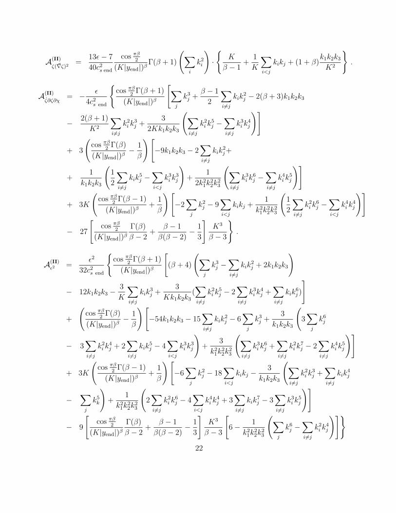
A(II)

ζ(~∇ζ)2=

13ε− 7

40c2s end

cos πβ2

(K|yend|)βΓ(β + 1)

(∑i

k2i

)·

{K

β − 1+

1

K

∑i<j

kikj + (1 + β)k1k2k3K2

}.

A(II)

ζ∂ζ∂χ= − ε

4c2s end

{cos πβ

2Γ(β + 1)

(K|yend|)β

[∑j

k3j +β − 1

2

∑i 6=j

kik2j − 2(β + 3)k1k2k3

− 2(β + 1)

K2

∑i 6=j

k2i k3j +

3

2Kk1k2k3

(∑i 6=j

k2i k5j −

∑i 6=j

k3i k4j

)]

+ 3

(cos πβ

2Γ(β)

(K|yend|)β− 1

β

)[−9k1k2k3 − 2

∑i 6=j

kik2j+

+1

k1k2k3

(1

2

∑i 6=j

kik5j −

∑i<j

k3i k3j

)+

1

2k21k22k

23

(∑i 6=j

k3i k6j −

∑i 6=j

k4i k5j

)]

+ 3K

(cos πβ

2Γ(β − 1)

(K|yend|)β+

1

β

)[−2∑j

k2j − 9∑i<j

kikj +1

k21k22k

23

(1

2

∑i 6=j

k2i k6j −

∑i<j

k4i k4j

)]

− 27

[cos πβ

2

(K|yend|)βΓ(β)

β − 2+

β − 1

β(β − 2)− 1

3

]K3

β − 3

}.

A(II)

ε2 =ε2

32c2s end

{cos πβ

2Γ(β + 1)

(K|yend|)β

[(β + 4)

(∑j

k3j −∑i 6=j

kik2j + 2k1k2k3

)

− 12k1k2k3 −3

K

∑i 6=j

kik3j +

3

Kk1k2k3(∑i 6=j

k2i k5j − 2

∑i 6=j

k3i k4j +

∑i 6=j

kik6j )

]

+

(cos πβ

2Γ(β)

(K|yend|)β− 1

β

)[−54k1k2k3 − 15

∑i 6=j

kik2j − 6

∑j

k3j +3

k1k2k3

(3∑j

k6j

− 3∑i 6=j

k2i k4j + 2

∑i 6=j

kik5j − 4

∑i<j

k3i k3j

)+

3

k21k22k

23

(∑i 6=j

k3i k6j +

∑i 6=j

k2i k7j − 2

∑i 6=j

k4i k5j

)]

+ 3K

(cos πβ

2Γ(β − 1)

(K|yend|)β+

1

β

)[−6∑j

k2j − 18∑i<j

kikj −3

k1k2k3

(∑i 6=j

k2i k3j +

∑i 6=j

kik4j

−∑j

k5k

)+

1

k21k22k

23

(2∑i 6=j

k2i k6j − 4

∑i<j

k4i k4j + 3

∑i 6=j

kik7j − 3

∑i 6=j

k3i k5j

)]

− 9

[cos πβ

2

(K|yend|)βΓ(β)

β − 2+

β − 1

β(β − 2)− 1

3

]K3

β − 3

[6− 1

k21k22k

23

(∑j

k6j −∑i 6=j

k2i k4j

)]}22

A(II)redef = −3(1 + ε)

10c2s end

[∑j

k3j

], (7.39)

where A(II)redef arises from the field redefinition (7.14) (2).

Note that the expressions in Case I and II take nearly identical form in the limit of small

sound speed, under the replacement α ↔ β. The only significant difference is the overall factor

of c−2s in Case I compared to c2s end(|yend|K)β in Case II, which stems from the power spectrum

being normalized at horizon-crossing and at the end of the contracting phase in Cases I and II,

respectively.

8 Non-Gaussian Signatures

In this Section, we discuss three observable features of the 3-point function, each of which can

distinguish the expanding branch from the contracting branch: the amplitude, parametrized by

the fNL parameter; the spectral dependence, characterized by the tilt nNG; and the momentum

shape of the 3-point amplitude.

Because of the reduced sound speed the 3-point amplitude is relatively large and potentially

measurable by current or near-future CMB experiments. Interestingly, the fNL parameter is

generically negative in the expanding case (including DBI inflation) and positive in the contracting

case. In particular, this holds true for DBI lagrangians. Nevertheless, it is certainly possible to

construct models where this conclusion is altered.

In standard slow-roll inflation, including DBI, the quasi-de Sitter nature of the background

(ε, η � 1) and the near constancy of the sound speed (εs � 1) imply both a nearly scale-invariant

power spectrum as well as nearly scale invariant non-Gaussianities. In the generalized models

studied here, however, the scale invariance of the 2-point function is maintained by balancing

a relatively large ε against a correspondingly large εs. This cancellation fails at the three-point

level, leading to a strong scale dependence for non-Gaussianities. Here again the expanding and

contracting solutions generically have a different signal: the inflationary branch (Case I) leads to

a blue tilt for the 3-point amplitude, whereas the ekpyrotic branch (Case II) has a red tilt.

But the most striking difference comes from the shape of the non-Gaussianities. In the in-

flationary branch, the shape is predominantly of the equilateral type [23], which is characteristic

of inflationary models with low sound speed, as in DBI [25]. In the ekpyrotic branch, however,

remarkably the shape is predominantly local.

This stark contrast in shape arises from the different behavior of ζ on super-horizon scales.

Because ζ tends to a constant outside the horizon in Case I, non-linearities can only grow for

2We are grateful to D. Baumann for pointing out important typos in an earlier version of this equation. The

corrected expression appeared in [56]

23

a finite period until modes exit the horizon. Thus non-Gaussianities peak when all wavevectors

have magnitude comparable to the Hubble radius, and therefore comparable to one another —

hence the equilateral shape. In Case II, ζ keeps growing outside the horizon, thereby allowing

non-linearities to grow until the end of the scaling phase. The non-Gaussian amplitude therefore

peaks when one of the wavenumbers is small, corresponding to the squeezed-triangle limit.

There is also an interesting subdominant contribution to the non-Gaussianities. While this is

suppressed by slow-roll parameters in standard DBI inflation, here it accounts for a more significant

fraction of the amplitude since ε can be relatively large in Case I. In the inflationary branch, we

find that the subdominant contribution is of the squashed shape; in the ekpyrotic branch, it is of

the equilateral shape.

8.1 Amplitude of Non-Gaussianities

The 3-point amplitude is characterized as usual by the fNL parameter [27]:

ζ = ζg(x) +3

5fNLζ

2g . (8.1)

Here we follow the WMAP sign convention, where positive fNL physically corresponds to negative-

skewness for the temperature fluctuations. The resulting 3-point function in momentum space is

given by

〈ζ(k1)ζ(k2)ζ(k3)〉 = (2π)7δ3(k1 + k2 + k3)P2ζ

3

10fNL

Σjk3j

Πjk3j, (8.2)

which peaks in the squeezed limit, e.g., k1 � k2, k3.

Although the momentum dependence of our amplitudes is manifestly different, in particular

peaking in the equilateral limit in Case I, it is conventional to define fNL by matching amplitudes

at k1 = k2 = k3 = K/3:

fNL = 30Ak1=k2=k3

K3. (8.3)

In the expanding case, by evaluating the right-hand side for the amplitudes listed in Sec. 7.4,

we obtain

f(I)NL =

35

108− 40

243(α + 4)

− 10

9c2s(α + 4)cos

απ

2Γ(1 + α)

{2

27(α + 1)(α + 2) (fX − 1) +

7

6(1 + α) +

9α2

32

}. (8.4)

To gain some intuition on the parametric dependence, a useful fitting formula for this expression

is

f(I)NL ≈ 0.27− 0.164 c−2s − (0.12 + 0.04fX) c−2s (1 + α) , (8.5)

24

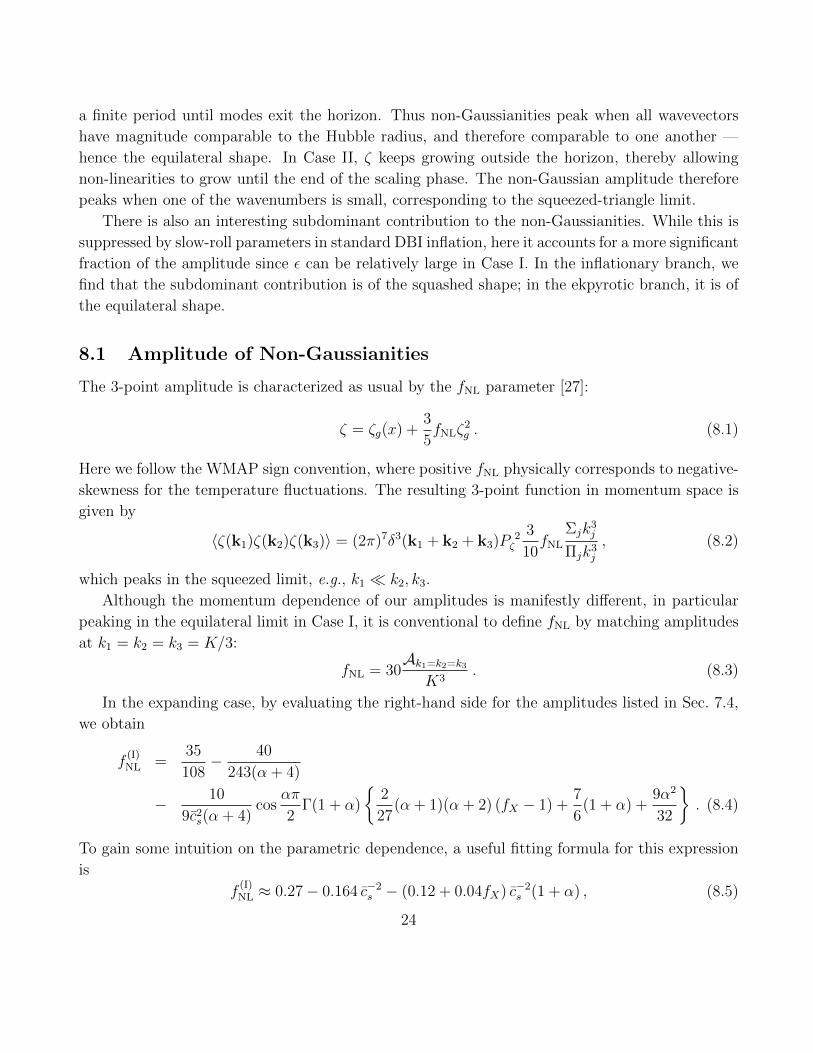
where we recall from (7.20) that −2 < α < 0 for 0 < ε < 1. Note that fNL is fairly insensitive to

fX , for reasonable values of this parameter, including DBI. Figure 1 compares the fitting formula

with the exact expression as a function of α and for various values of fX . The agreement is

typically within 10 % over the phenomenologically allowed range of ε . 0.3 (or α ∼> − 1).

-1.0 -0.8 -0.6 -0.4 -0.2 0.0-30

-25

-20

-15

-10

-5

0

Α

f NLHIL

Figure 1: Comparison between the exact formula (8.4) and its linear fitting (8.5) in the expanding

case, for the parameter region of interest: −1 < α < 0. Values of f(I)NL are evaluated as a function of

α for different cs and fX : from top to bottom, (cs, fX) = (0.25, 1); (0.15, 0.1); (0.12, 0.9); (0.1, 0.1).

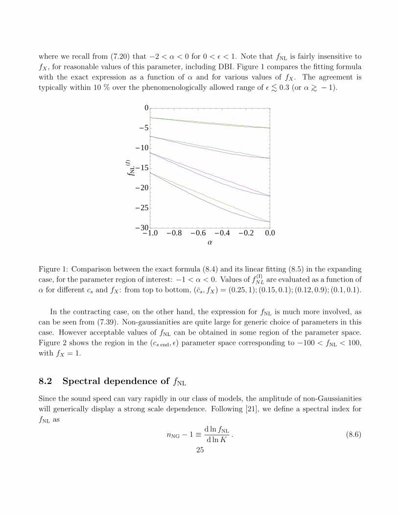
In the contracting case, on the other hand, the expression for fNL is much more involved, as

can be seen from (7.39). Non-gaussianities are quite large for generic choice of parameters in this

case. However acceptable values of fNL can be obtained in some region of the parameter space.

Figure 2 shows the region in the (cs end, ε) parameter space corresponding to −100 < fNL < 100,

with fX = 1.

8.2 Spectral dependence of fNL

Since the sound speed can vary rapidly in our class of models, the amplitude of non-Gaussianities

will generically display a strong scale dependence. Following [21], we define a spectral index for

fNL as

nNG − 1 ≡ d ln fNL

d lnK. (8.6)

25

0.2 0.4 0.6 0.8 1.02.0

2.2

2.4

2.6

2.8

3.0

cs

Ε

Figure 2: In the (cs end, ε) plane we plot the region corresponding to fNL < 100 with the choice

fX = 1. The upper curve corresponds to the upper bound fNL = 100.

In Case I, the non-Gaussian tilt arises from the c−2s prefactors in (8.5). For small values of the

sound speed, we obtain

(nNG − 1)I ≈ −2d ln csd lnK

= −α . (8.7)

And since −2 < α < 0 within the inflationary range 0 < ε < 1, we get a blue tilt for the 3-point

function in the expanding branch, corresponding to larger non-Gaussian amplitude on smaller

scales. As discussed in Sec. 4.2, the present range of observable scales goes from the largest

(CMB) ones down to typical galactic sizes: Kgal/KCMB ' 103. We therefore expect

f(I)NL(CMB) ≈ 103αf

(I)NL(gal) . (8.8)

Clearly we must require that non-Gaussianities are within the perturbative regime down to galactic

scales, i.e., f(I)NL(gal) . 104. In the observationally-optimistic scenario in which large-scale non-

Gaussianities are of the order of the present experimental limits (|fNL(CMB)| ∼ 100) this implies

|α| . 2/3 (ε . 1/5). Our model is less constrained if we assume instead |fNL(CMB)| = O(1), in

which case |α| . 4/3 (ε . 1/2).

The tilt is also important in Case II. In this case, however, it cannot be approximated as

constant over the relevant range of scales, since not all terms in (7.39) share a common (|yend|K)β

prefactor.

26

0.5

1

x2

0

1

x30

10

20

(a) −A(I)(1, x2, x3)/(x2x3) for α = −0.3

0.5

1

x2

0

1

x30

5

10

15

(b) −A(I)(1, x2, x3)/(x2x3) for α = −0.9

0.5

1

x20

1

x3

0

0.02

0.04

(c) |A(I) −Aequi|/(x2x3) for α = −0.3

0.5

1

x20

1

x3

0

0.1

0.2

(d) |A(I) −Aequi|/(x2x3) for α = −0.9

Figure 3: In the top two panels we plot the non-Gaussian ampitude in the inflationary branch,

−A(I)(1, x2, x3)/(x2x3) for cs = 0.1, fX = 0.9, α = −0.3 (ε = 0.08, top left) and α = −0.9 (ε = 0.3,

top right). Thus the dominant contribution peaks for equilateral configurations (x2 ≈ x3 ≈ 1).

To see how this differs from DBI inflation, in the bottom two panels we subtract the dominant

DBI-like (equilateral) contribution and plot |A(I) − Aequi|/(x2x3), where A(I) and Aequi have each

been normalized to one in the equilateral limit x2 = x3 = 1. Thus the subdominant contribution

peaks for squashed configurations (x2 ≈ x3 ≈ 0.5).

27

8.3 Shape of non-Gaussianities

In light of the substantial running of the three-point function, we study the shape of the amplitude

at fixed K, thereby disentangling shape and running effects. Following the literature [23], it is

convenient to focus on the dimensionless ratio A/k1k2k3. We will plot this quantity A/k1k2k3 in

the x2-x3 plane, where x2 = k2/k1 and x3 = k3/k1. Moreover, we can restrict ourselves to the

range 1− x2 ≤ x3 ≤ x2, where the first inequality is the triangle inequality while the second one

avoids plotting the same configuration twice.

Starting with the expanding case, it is instructive to first consider the limit ε→ 0 (α→ 0). In

this regime, the last two terms in (7.38) are subdominant and, save for the A(I)

ζ3contribution, our

shape reduces to the equilateral shape

Aequi ∝1

8

∑i

k3i −1

K

∑i<j

k2i k2j +

1

2K2

∑i 6=j

k2i k3j . (8.9)

Now, even though each term above when divided by k1k2k3 is singular in the degenerate limit

k3 → 0, all divergences remarkably cancel each other in the combination (8.9). One can in fact

check that the cancellation works in the full set of amplitudes (7.38) for any value of ε (α), despite

other potentially divergent terms such as∑

i 6=j kik2j and

∑i k

4i . This is a consequence of the

consistency relation [33] A/(k1k2k3) ' (ns− 1)k1/k3 for the three-point function in the local limit

k3 � k1 = k2, which in this case predicts vanishing amplitude since ns = 1. Therefore, the total

amplitude peaks in the equilateral limit k1 ≈ k2 ≈ k3 for a generic choice of parameters, as shown

in the top two panels of Fig. 3, and the shape is predominantly of the equilateral type. This shape

is generally expected in models with c2s < 1 and where higher derivatives operators are present in

the effective action because of the shorter Jeans Length of the perturbations that easily produce

non-linearities on shorter scales.

Nevertheless, the shape in Case I is not exactly of the form (8.9). We can unearth subdominant

contributions by subtracting the equilateral shape (8.9) normalized at the equilateral point k1 =

k2 = k3. The resulting amplitude, shown in the bottom two panels in Fig. 3, peaks for “squashed”

triangles. This subdominant contribution is of course also present in standard DBI inflation, albeit

suppressed by slow roll parameters. Because our mechanism allows for much larger values of ε,

the squashed amplitude is correspondingly more important here.

These statements can be made more quantitative by looking at the scalar product between

shapes A1 · A2, introduced by [23]

A1 · A2 =∑~ki

A1(k1, k2, k3)A2(k1, k2, k3)/(σ2k1σ2k2σ2k3

) . (8.10)

The corresponding angle θ12 therefore informs us on how different and distinguishable the two

28

-1.0 -0.8 -0.6 -0.4 -0.2 0.0

0.02

0.04

0.06

0.08

0.10

0.12

Α

ΘI-equi

-1.0 -0.8 -0.6 -0.4 -0.2 0.00.00

0.05

0.10

0.15

0.20

Α

ΘI-equi

Figure 4: The angle θ defined in eq. (8.11) is plotted as a function of α in the expanding case. In

the left panel cs = 0.05 and fX = 0.5, in the right panel we choose instead cs = 0.5 and fX = 0.5.

The distinguishability between our shape and DBI’s increases with |α| and with cs.

shapes are:

cos(θ12) =A1 · A2

(A1 · A1)1/2(A2 · A2)1/2. (8.11)

In Fig. 4 we plot the angle above calculated between A(I) and Aequi as a function of the parameter

α. As expected, the difference between the shapes increases with |α|.

0.6

0.8

1.0

0.0

0.5

1.0

0

500

(a) −A(II)(1, x2, x3)/(x2x3) for β = 0.1

0.6

0.8

1.0

0.0

0.5

1.0

0

100

(b) −A(II)(1, x2, x3)/(x2x3) for β = −0.1

Figure 5: We plot A(II)(1, x2, x3)/(x2x3) for cs end = .95, fX = 1, β = 0.1 (left) and cs end = .9,

β = 0.01 (right).

In the contracting case, as described earlier, the curvature perturbation keeps growing outside

29

the horizon, resulting in non-Gaussianities that peak in the squeezed limit, as shown in Fig. 5.

Note, however, that the amplitude as k3 � k1, k2, corresponding to squeezed configurations, is

more singular than the local form:

ALoc ∝∑i

k3i . (8.12)

This traces back to higher powers of ki in the denominator of (7.39). In particular, non-Gaussianity

in the contracting case manifestly violates Maldacena’s consistency relation, which assumes that

ζ(k3) tends to a constant at long wavelengths and therefore behaves as a background wave for the

short-wavelengths modes. This assumption does not hold in this case, while the reversed argument

is probably the correct explanation for our shape a local type: precisely because ζ(k3) keeps

growing outside the horizon the short wavelength modes effectively “feel” a different background

evolution. The strong peak in the squeezed limit obtained here is remarkable since non-Gaussianity

of this type usually results from entropy perturbations between two scalar degrees of freedom, such

as in the curvaton [14], modulated reheating [28], pre-big bang pump field [10] and New Ekpyrotic

mechanisms [6, 29, 30, 31].

9 Conclusion

The near scale invariance of the primordial spectrum estalished by CMB and large scale structure

observations is widely hailed as evidence for a phase of quasi de Sitter expansion in the early

universe. In this paper we have shown that a suitably time-dependent sound speed allows for a

much richer spectrum of early universe cosmologies, including both expanding [17] and contracting

backgrounds.

In the expanding case, this mechanism was first proposed by [17, 18, 19], who considered a

universe with an extremely large sound speed initially. Unlike [18] we have restricted ourselves to

subluminal sound speed throughout. Thus the background must still be inflationary in order for

perturbations to be stretched outside the physical horizon. Inflationary expansion of course has

the added virtue of making the universe flat, homogeneous and isotropic. Our mechanism in this

case alleviates the usual slow-roll conditions, from the restrictive ε . 1/60 to ε . 0.3.

In the contracting branch, requiring that the background addresses the flatness and homo-

geneity problems of standard big bang cosmology leads to the ekpyrotic regime ε > 3 (or w > 1).

Unlike the New Ekpyrotic mechanism which relies on two scalar fields, here a single scalar degree

of freedom is sufficient to endow ζ with a scale invariant spectrum.

The phenomenology of non-Gaussianities is very rich and offers many distinguishing features.

To start with, the cancelation mechanism between the sound speed and the cosmological equation

of state does not carry over to the three-point function. Hence non-Gaussianities display a strong

scale dependence, peaking on small scales in the inflationary branch and on large scales in the

30

ekpyrotic branch.

Moreover, the shape of the amplitude is drastically different in each case. In the expanding

case, the amplitude is predominantly of the equilateral type, as usual with low sound speed models,

such as DBI inflation. In the contracting case, it is predominantly of the local form, peaking for

squeezed triangles. This contrast in shape arises because ζ has different behaviors on super-

horizon scales: whereas it tends to a constant as usual in the inflationary case, it keeps growing

in the ekpyrotic branch. Beneath the dominant shape lies a subdominant contribution, which can

make up as much as 10% of the total amplitude. This subdominant piece peaks for squashed and

equilateral triangles in the inflationary and ekpyrotic branches, respectively.

Many offspring projects naturally suggest themselves. Firstly, while our study of the non-

Gaussianity focused on P (X,φ) scalar lagrangians, it would be interesting to consider the more

general effective field theory framework proposed in [57]. From this point of view, the P (X,φ)

predictions are a subset of all possible results — hence we expect a wider spectrum of non-

Gaussian features. Secondly, in light of the abundance of non-Gaussian features in our class

of models, it will be enlightning to investigate the potential of near-future experiments such as

Planck to detect some of the signatures described here, such as the strong title and the distinctive

shapes. Moreover, we should push the non-Gaussian exploration further and calculate higher-

point correlation functions in this framework. The shape and tilt of the trispectrum should offer

more ways to break degeneracies between the different cosmologies studied here.

Acknowledgments We thank Niayesh Afshordi, Robert Brandenberger, Maurizio Gasperini,

Jean-Luc Lehners, Alberto Nicolis, Leonardo Senatore, Paul Steinhardt, Gabriele Veneziano, Ma-

tias Zaldarriaga and especially Andrew Tolley for many helpful discussions. We are grateful to

Daniel Baumann for helpful feedback and for pointing out important typos in the original version

of Eq. (7.39). The research of J.K. and F.P. at the Perimeter Institute is supported in part by the

Government of Canada through NSERC and by the Province of Ontario through the Ministry of

Research & Innovation.

A Explicit DBI Examples

In this Section, we present explicit realizations of the scaling solutions described so far, closely

following the analysis of [39]. We focus on DBI lagrangians:

LDBI = −f−1(φ)√

1 + f(φ)(∂φ)2 + f−1(φ)− V (φ) , (A.1)

31

where f(φ) describes the warp factor of the throat within which the 3-brane is moving. The

cosmological equations are

3H2M2Pl =

c−1s − 1

f+ V ;

d lnH

dN= − 1

2M2Plcs

(dφ

dN

)2

, (A.2)

where dN ≡ Hdt, and cs is given in (7.7).

Our goal is to determine the form of f(φ) and V (φ) corresponding to the scaling solutions of

interest. To begin with, along the solution cs ∼ eεsN , it is useful to think of cs as a function of the

classical solution for φ. Thus,

εs =d ln cs(φ)

dφ

dφ

dN= ±√

2ε

c1/2s

dcsdφ

MPl , (A.3)

where in the last step we have used (A.2). And since εs is assumed constant, this can be integrated

at once for cs(φ):

cs(φ) =ε2s8ε

φ2

M2Pl

. (A.4)

Note that we have chosen the integration constant such that the sound speed vanishes when φ = 0.

Similarly, on the background solution we can think of H as a function of φ(N). Proceeding

along similar lines as (A.3), ε can be expressed as

ε = 2M2Plcs

(d lnH

dφ

)2

. (A.5)

And substituting for cs(φ) yields a differential equation for the Hubble parameter: d lnH/d lnφ =

±2ε/εs, which easily integrates to

H(φ) ∼ φ−2ε/εs . (A.6)

Noting that εs < 0 in both Cases I and II — in Case II, this assumes ε > 3/2 —, we have chosen

the sign so that |H| decreases (increases) in the expanding (contracting) case.

Having obtained expressions for cs(φ) and H(φ), we can solve (A.2) for the potential and warp

factor:

V (φ) = 3H2(φ)M2Pl

(1− 2ε

3(1 + cs(φ))

). (A.7)

Explicitly, this gives

V (φ) = V0

(φ

MPl

)−4ε/εs1− 2ε

3

1

1 + ε2sφ2

8εM2Pl

, (A.8)

32

where V0 is a constant. For Case I, where εs = −2ε, and in the limit of small sound speed

(φ�MPl), this gives

VI(φ) ≈ V0

(1− 2ε

3

)φ2

M2Pl

. (A.9)

Meanwhile, for Case II, where εs = 2(3− 2ε)/5,

VII(φ) ≈ −V0(

2ε

3− 1

)(φ

MPl

)10ε/(2ε−3)

. (A.10)

Similarly, the warp factor can be expressed as

f(φ) =1− c2s(φ)

2εH2(φ)M2Plcs(φ)

, (A.11)

which, for our explicit solutions, reduces to

f(φ) =12

V0ε2s

(φ

MPl

) 4εεs−2(

1− ε4sφ4

64ε2M4Pl

). (A.12)

Again in the limit of small sound speed, we obtain, respectively for Case I and II,

fI(φ) ∼(

φ

MPl

)−4;

fII(φ) ∼(

φ

MPl

)−2 7ε−32ε−3

. (A.13)

Thus the desired potentials and warp factors are approximately power-law in form. Note that

in Case I we have reproduced the potential and AdS warp factor of [25]. The exponents in V (φ)

and f(φ) are independent of ε in this case.

B Relevant Integrals

Below are the integrals used in the calculations of Section 7 for Case II.

Im

{∫ yend

−∞dy

H

c5/2s

1− iKyy4

eiKy}

= −Hend

c5/2s end

K3

β − 3

[cos πβ

2

(K|yend|)βΓ(β)

β − 2+

β − 1

β(β − 2)− 1

3

](B.1)

Im

{∫ yend

−∞dy

H

c1/2s

1− iKyy4

eiKy}

= −Hend

c1/2s end

K3

9(B.2)

Im

{∫ yend

−∞dy

H

c5/2s

eiKy

y2

}=Hend

c5/2s end

K

[cos πβ

2

(K|yend|)βΓ(β − 1) +

1

β

](B.3)

33

Im

{∫ yend

−∞dy

H

c1/2s

eiKy

y2

}= −Hend

c1/2s end

K

3(B.4)

Im

{i

∫ yend

−∞dy

H

c5/2s

eiKy

y

}= −Hend

c5/2s end

[cos πβ

2

(K|yend|)βΓ(β)− 1

β

](B.5)

Im

{i

∫ yend

−∞dy

H

c1/2s

eiKy

y

}= −1

3

Hend

c1/2s end

(B.6)

Im

{∫ yend

−∞dy

H

c5/2s

eiKy}

= −Hend

c5/2s end

1

K

cos πβ2

(K|yend|)βΓ(β + 1) (B.7)

Im

{∫ yend

−∞dy

H

c1/2s

eiKy}∼ (Kyend)2 =⇒ subleading (B.8)

Im

{i

∫ yend

−∞dy

H

c5/2s

yeiKy}

=Hend

c5/2s end

1

K2

cos πβ2

(K|yend|)βΓ(β + 2) (B.9)

Im

{i

∫ yend

−∞dy

H

c1/2s

yeiKy}∼ (Kyend)2 =⇒ subleading (B.10)

Im

{∫ yend

−∞dy

H

c5/2s

y2eiKy}

=Hend

c5/2s end

1

K3

cos πβ2

(K|yend|)βΓ(β + 3) (B.11)

Im

{∫ yend

−∞dy

H

c1/2s

y2eiKy}∼ (Kyend)2 =⇒ subleading (B.12)

Im

{i

∫ yend

−∞dy

H

c5/2s

y3eiKy}

= −Hend

c5/2s end

1

K4

cos πβ2

(K|yend|)βΓ(β + 4) . (B.13)

References

[1] F. Finelli and R. Brandenberger, “On the generation of a scale-invariant spectrum of adiabatic

fluctuations in cosmological models with a contracting phase,” Phys. Rev. D 65, 103522

(2002) [arXiv:hep-th/0112249]; D. Wands, “Duality invariance of cosmological perturbation

spectra,” Phys. Rev. D 60, 023507 (1999) [arXiv:gr-qc/9809062].

[2] S. Gratton, J. Khoury, P. J. Steinhardt and N. Turok, “Conditions for generating scale-

invariant density perturbations,” Phys. Rev. D 69, 103505 (2004) [arXiv:astro-ph/0301395].

[3] E. I. Buchbinder, J. Khoury and B. A. Ovrut, “New Ekpyrotic Cosmology,” Phys. Rev. D

76, 123503 (2007) [arXiv:hep-th/0702154].

[4] F. Finelli, “Assisted contraction,” Phys. Lett. B 545, 1 (2002) [arXiv:hep-th/0206112]; S. Tsu-

jikawa, R. Brandenberger and F. Finelli, “On the construction of nonsingular pre-big-bang

34

and ekpyrotic cosmologies and the resulting density perturbations,” Phys. Rev. D 66, 083513

(2002) [arXiv:hep-th/0207228].

[5] J. L. Lehners, P. McFadden, N. Turok and P. J. Steinhardt, “Generating ekpyrotic curvature

perturbations before the big bang,” Phys. Rev. D 76, 103501 (2007) [arXiv:hep-th/0702153].

[6] P. Creminelli and L. Senatore, “A smooth bouncing cosmology with scale invariant spectrum,”

JCAP 0711, 010 (2007) [arXiv:hep-th/0702165].

[7] K. Koyama and D. Wands, “Ekpyrotic collapse with multiple fields,” JCAP 0704, 008

(2007) [arXiv:hep-th/0703040]; K. Koyama, S. Mizuno and D. Wands, “Curvature pertur-

bations from ekpyrotic collapse with multiple fields,” Class. Quant. Grav. 24, 3919 (2007)

[arXiv:0704.1152 [hep-th]].

[8] A. Notari and A. Riotto, “Isocurvature perturbations in the ekpyrotic universe,” Nucl. Phys.

B 644, 371 (2002) [arXiv:hep-th/0205019].

[9] G. Veneziano, “Scale Factor Duality For Classical And Quantum Strings,” Phys. Lett. B 265,

287 (1991); M. Gasperini and G. Veneziano, “Pre - big bang in string cosmology,” Astropart.

Phys. 1, 317 (1993) [arXiv:hep-th/9211021].

[10] E. J. Copeland, R. Easther and D. Wands, “Vacuum fluctuations in axion-dilaton cosmolo-

gies,” Phys. Rev. D 56, 874 (1997) [arXiv:hep-th/9701082]; E. J. Copeland, J. E. Lidsey and

D. Wands, “S-duality-invariant perturbations in string cosmology,” Nucl. Phys. B 506, 407

(1997) [arXiv:hep-th/9705050]; E. J. Copeland, A. Lahiri and D. Wands, “Low-energy effec-

tive string cosmology,” Phys. Rev. D 50, 4868 (1994) [arXiv:hep-th/9406216]; E. J. Copeland,

A. Lahiri and D. Wands, “String cosmology with a time dependent antisymmetric ten-

sor potential,” Phys. Rev. D 51, 1569 (1995) [arXiv:hep-th/9410136]; M. Gasperini and

G. Veneziano, “Constraints on pre-big bang models for seeding large-scale anisotropy by

massive Kalb-Ramond axions,” Phys. Rev. D 59, 043503 (1999) [arXiv:hep-ph/9806327].

[11] J. L. Lehners, “Ekpyrotic and Cyclic Cosmology,” Phys. Rept. 465, 223 (2008)

[arXiv:0806.1245 [astro-ph]].

[12] M. Gasperini and G. Veneziano, “The pre-big bang scenario in string cosmology,” Phys. Rept.

373, 1 (2003) [arXiv:hep-th/0207130].

[13] S. Mollerach, “Isocurvature Baryon Perturbations And Inflation,” Phys. Rev. D 42, 313

(1990).

35

[14] D. H. Lyth and D. Wands, “Generating the curvature perturbation without an inflaton,”

Phys. Lett. B 524, 5 (2002) [arXiv:hep-ph/0110002]; K. Enqvist and M. S. Sloth, “Adia-

batic CMB perturbations in pre big bang string cosmology,” Nucl. Phys. B 626, 395 (2002)

[arXiv:hep-ph/0109214]; T. Moroi and T. Takahashi, “Effects of cosmological moduli fields

on cosmic microwave background,” Phys. Lett. B 522, 215 (2001) [Erratum-ibid. B 539, 303

(2002)] [arXiv:hep-ph/0110096].

[15] V. Bozza, M. Gasperini, M. Giovannini and G. Veneziano, “Assisting pre-big bang

phenomenology through short-lived axions,” Phys. Lett. B 543, 14 (2002) [arXiv:hep-

ph/0206131]; V. Bozza, M. Gasperini, M. Giovannini and G. Veneziano, “Constraints on

pre-big bang parameter space from CMBR anisotropies,” Phys. Rev. D 67, 063514 (2003)

[arXiv:hep-ph/0212112].

[16] M. Gasperini, “Tensor perturbations in high-curvature string backgrounds,” Phys. Rev. D

56, 4815 (1997) [arXiv:gr-qc/9704045].

[17] C. Armendariz-Picon and E. A. Lim, “Scale invariance without inflation?,” JCAP 0312, 002

(2003) [arXiv:astro-ph/0307101]; C. Armendariz-Picon, “Near scale invariance with modified

dispersion relations,” JCAP 0610, 010 (2006) [arXiv:astro-ph/0606168].

[18] J. Magueijo, “Speedy sound and cosmic structure,” Phys. Rev. Lett. 100, 231302 (2008)

[arXiv:0803.0859 [astro-ph]].

[19] Y. S. Piao, “Seeding of Primordial Perturbations During a Decelerated Expansion,” Phys.

Rev. D 75, 063517 (2007) [arXiv:gr-qc/0609071].

[20] A. Adams, N. Arkani-Hamed, S. Dubovsky, A. Nicolis and R. Rattazzi, “Causality, analyticity

and an IR obstruction to UV completion,” JHEP 0610, 014 (2006) [arXiv:hep-th/0602178].

[21] X. Chen, “Running non-Gaussianities in DBI inflation,” Phys. Rev. D 72, 123518 (2005)

[arXiv:astro-ph/0507053].

[22] M. LoVerde, A. Miller, S. Shandera and L. Verde, “Effects of Scale-Dependent Non-

Gaussianity on Cosmological Structures,” JCAP 0804, 014 (2008) [arXiv:0711.4126 [astro-

ph]].

[23] D. Babich, P. Creminelli and M. Zaldarriaga, “The shape of non-Gaussianities,” JCAP 0408,

009 (2004) [arXiv:astro-ph/0405356].

[24] E. Silverstein and D. Tong, “Scalar speed limits and cosmology: Acceleration from D-

cceleration,” Phys. Rev. D 70, 103505 (2004) [arXiv:hep-th/0310221].

36

[25] M. Alishahiha, E. Silverstein and D. Tong, “DBI in the sky,” Phys. Rev. D 70, 123505 (2004)

[arXiv:hep-th/0404084].

[26] X. Chen, M. x. Huang, S. Kachru and G. Shiu, “Observational signatures and non-

Gaussianities of general single field inflation,” JCAP 0701, 002 (2007) [arXiv:hep-

th/0605045].

[27] E. Komatsu and D. N. Spergel, “Acoustic signatures in the primary microwave background

bispectrum,” Phys. Rev. D 63, 063002 (2001) [arXiv:astro-ph/0005036].

[28] G. Dvali, A. Gruzinov and M. Zaldarriaga, “A new mechanism for generating density pertur-

bations from inflation,” Phys. Rev. D 69, 023505 (2004) [arXiv:astro-ph/0303591]; L. Kofman,

“Probing string theory with modulated cosmological fluctuations,” arXiv:astro-ph/0303614.

[29] E. I. Buchbinder, J. Khoury and B. A. Ovrut, “Non-Gaussianities in New Ekpyrotic Cosmol-

ogy,” Phys. Rev. Lett. 100, 171302 (2008) [arXiv:0710.5172 [hep-th]].

[30] K. Koyama, S. Mizuno, F. Vernizzi and D. Wands, “Non-Gaussianities from ekpyrotic collapse

with multiple fields,” JCAP 0711, 024 (2007) [arXiv:0708.4321 [hep-th]].

[31] J. L. Lehners and P. J. Steinhardt, “Non-Gaussian Density Fluctuations from Entropically

Generated Curvature Perturbations in Ekpyrotic Models,” Phys. Rev. D 77, 063533 (2008)

[arXiv:0712.3779 [hep-th]]; “Intuitive understanding of non-gaussianity in ekpyrotic and cyclic

models,” Phys. Rev. D 78, 023506 (2008) [arXiv:0804.1293 [hep-th]].

[32] D. S. Salopek and J. R. Bond, “Stochastic inflation and nonlinear gravity,” Phys. Rev. D 43,

1005 (1991).

[33] J. M. Maldacena, “Non-Gaussian features of primordial fluctuations in single field inflationary

models,” JHEP 0305, 013 (2003) [arXiv:astro-ph/0210603].

[34] J. M. Bardeen, P. J. Steinhardt and M. S. Turner, “Spontaneous Creation Of Almost Scale -

Free Density Perturbations In An Inflationary Universe,” Phys. Rev. D 28, 679 (1983).

[35] D. H. Lyth, K. A. Malik and M. Sasaki, “A general proof of the conservation of the curvature

perturbation,” JCAP 0505, 004 (2005) [arXiv:astro-ph/0411220].

[36] A. J. Tolley and D. H. Wesley, “Scale-invariance in expanding and contracting universes from

two-field models,” JCAP 0705, 006 (2007) [arXiv:hep-th/0703101].

[37] E. I. Buchbinder, J. Khoury and B. A. Ovrut, “On the Initial Conditions in New Ekpyrotic

Cosmology,” JHEP 0711, 076 (2007) [arXiv:0706.3903 [hep-th]].

37

[38] J. K. Erickson, D. H. Wesley, P. J. Steinhardt and N. Turok, “Kasner and mixmaster behavior

in universes with equation of state w ≥ 1,” Phys. Rev. D 69, 063514 (2004) [arXiv:hep-

th/0312009].

[39] W. H. Kinney and K. Tzirakis, “Quantum modes in DBI inflation: exact solutions and

constraints from vacuum selection,” Phys. Rev. D 77, 103517 (2008) [arXiv:0712.2043 [astro-

ph]].

[40] J. Garriga and V. F. Mukhanov, “Perturbations in k-inflation,” Phys. Lett. B 458, 219 (1999)

[arXiv:hep-th/9904176].

[41] E. M. Lifshitz and I. M. Khalatnikov, “Investigations in relativistic cosmology,” Adv. Phys.

12, 185 (1963); V. A. Belinsky, I. M. Khalatnikov and E. M. Lifshitz, “Oscillatory approach

to a singular point in the relativistic cosmology,” Adv. Phys. 19, 525 (1970).

[42] J. Demaret, M. Henneaux and P. Spindel, “Nonoscillatory Behavior In Vacuum Kaluza-

Klein Cosmologies,” Phys. Lett. B 164, 27 (1985); T. Damour and M. Henneaux, “Chaos in

superstring cosmology,” Phys. Rev. Lett. 85, 920 (2000) [arXiv:hep-th/0003139]; T. Damour

and M. Henneaux, “E(10), BE(10) and arithmetical chaos in superstring cosmology,” Phys.

Rev. Lett. 86, 4749 (2001) [arXiv:hep-th/0012172]; T. Damour, M. Henneaux and H. Nicolai,

“Cosmological billiards,” Class. Quant. Grav. 20, R145 (2003) [arXiv:hep-th/0212256].

[43] J. Khoury, B. A. Ovrut, P. J. Steinhardt and N. Turok, “The ekpyrotic universe: Colliding

branes and the origin of the hot big bang,” Phys. Rev. D 64, 123522 (2001) [arXiv:hep-

th/0103239].

[44] J. Khoury, B. A. Ovrut, N. Seiberg, P. J. Steinhardt and N. Turok, “From big crunch to big

bang,” Phys. Rev. D 65, 086007 (2002) [arXiv:hep-th/0108187].

[45] J. Khoury, B. A. Ovrut, P. J. Steinhardt and N. Turok, “Density perturbations in the

ekpyrotic scenario,” Phys. Rev. D 66, 046005 (2002) [arXiv:hep-th/0109050]; J. Khoury,

B. A. Ovrut, P. J. Steinhardt and N. Turok, “A brief comment on ’The pyrotechnic uni-

verse’,” arXiv:hep-th/0105212;

[46] A. J. Tolley, N. Turok and P. J. Steinhardt, “Cosmological perturbations in a big crunch /

big bang space-time,” Phys. Rev. D 69, 106005 (2004) [arXiv:hep-th/0306109].

[47] P. J. Steinhardt and N. Turok, “Cosmic evolution in a cyclic universe,” Phys. Rev. D 65,

126003 (2002) [arXiv:hep-th/0111098].

38

[48] T. J. Battefeld, S. P. Patil and R. H. Brandenberger, “On the transfer of metric fluctuations

when extra dimensions bounce or stabilize,” Phys. Rev. D 73, 086002 (2006) [arXiv:hep-

th/0509043].

[49] D. H. Lyth, “The primordial curvature perturbation in the ekpyrotic universe,” Phys. Lett.

B 524, 1 (2002) [arXiv:hep-ph/0106153]; ‘The failure of cosmological perturbation theory in

the new ekpyrotic scenario,” Phys. Lett. B 526, 173 (2002) [arXiv:hep-ph/0110007]; R. Dur-

rer, “Clarifying perturbations in the ekpyrotic universe: A web-note,” arXiv:hep-th/0112026;

R. Brandenberger and F. Finelli, “On the spectrum of fluctuations in an effective field the-

ory of the ekpyrotic universe,” JHEP 0111, 056 (2001) [arXiv:hep-th/0109004]; J. Martin,

P. Peter, N. Pinto Neto and D. J. Schwarz, “Passing through the bounce in the ekpyrotic

models,” Phys. Rev. D 65, 123513 (2002) [arXiv:hep-th/0112128]; J. c. Hwang, “Cosmological

structure problem in the ekpyrotic scenario,” Phys. Rev. D 65, 063514 (2002) [arXiv:astro-

ph/0109045].

[50] P. Creminelli, A. Nicolis and M. Zaldarriaga, “Perturbations in bouncing cosmologies:

Dynamical attractor vs scale invariance,” Phys. Rev. D 71, 063505 (2005) [arXiv:hep-

th/0411270].

[51] S. Alexander, T. Biswas and R. H. Brandenberger, “On the Transfer of Adiabatic Fluctuations

through a Nonsingular Cosmological Bounce,” arXiv:0707.4679 [hep-th].

[52] R. Brustein, M. Gasperini, M. Giovannini, V. F. Mukhanov and G. Veneziano, “Metric per-

turbations in dilaton driven inflation,” Phys. Rev. D 51, 6744 (1995) [arXiv:hep-th/9501066];

R. Brustein, M. Gasperini, M. Giovannini and G. Veneziano, “Relic gravitational waves

from string cosmology,” Phys. Lett. B 361, 45 (1995) [arXiv:hep-th/9507017]; M. Gasperini,

“Tensor perturbations in high-curvature string backgrounds,” Phys. Rev. D 56, 4815 (1997)

[arXiv:gr-qc/9704045].

[53] L. A. Boyle, P. J. Steinhardt and N. Turok, “The cosmic gravitational wave background in a

cyclic universe,” Phys. Rev. D 69, 127302 (2004) [arXiv:hep-th/0307170].

[54] F. Gmeiner and C. D. White, “DBI Inflation using a One-Parameter Family of Throat Ge-

ometries,” JCAP 0802, 012 (2008) [arXiv:0710.2009 [hep-th]].

[55] D. Seery and J. E. Lidsey, “Primordial non-gaussianities in single field inflation,” JCAP 0506,

003 (2005) [arXiv:astro-ph/0503692].

[56] D. Baumann, L. Senatore, M. Zaldarriaga, “Scale-Invariance and the Strong Coupling Prob-

lem,” [arXiv:1101.3320 [hep-th]].

39

[57] C. Cheung, P. Creminelli, A. L. Fitzpatrick, J. Kaplan and L. Senatore, “The Effective Field

Theory of Inflation,” JHEP 0803, 014 (2008) [arXiv:0709.0293 [hep-th]].

40