Rapid and Accurate Calculation Rapid and Accurate Calculation of the Voigt Functionof the Voigt Function

D. Chris BennerD. Chris BennerKendra L. LetchworthKendra L. Letchworth

9th International HITRAN Conference9th International HITRAN Conference June 26-28, 2006June 26-28, 2006

Why is this routine needed?Why is this routine needed?• Spectra with higher signal to noise ratios require more Spectra with higher signal to noise ratios require more

accurate analysis routines.accurate analysis routines.• Most fitting programs and simulations perform millions of Most fitting programs and simulations perform millions of

calculations, so routines must also be fast.calculations, so routines must also be fast.• Our routine calculates the Voigt profile to a relative accuracy Our routine calculates the Voigt profile to a relative accuracy

of 10of 10-6 -6 ..• 100 times more accurate than routines such as Drayson & 100 times more accurate than routines such as Drayson &

HumlHumlíčíček but requires 2 to 4 times less calculation time. ek but requires 2 to 4 times less calculation time. • Our routine includes the imaginary part of the function for Our routine includes the imaginary part of the function for

applications to line-mixing.applications to line-mixing.• Option of returning the derivatives of the real Voigt profile with Option of returning the derivatives of the real Voigt profile with

respect to x and y. They are calculated with relative accuracy respect to x and y. They are calculated with relative accuracy of less than 10of less than 10-3-3, without significant additional calculation time , without significant additional calculation time required.required.

• For more information about relative speed and accuracy of For more information about relative speed and accuracy of various Voigt routines (not including ours) see: various Voigt routines (not including ours) see:

F. Schreier, J.Q.S.R.T., Vol. 48, 1992.F. Schreier, J.Q.S.R.T., Vol. 48, 1992.

The Voigt ProfileThe Voigt Profile

),(),(),( yxiLyxKyxVoigt

dvvxy

vyyxK

22

2

)(

)exp(),(

dv

vxy

vvxyxL

22

2

)(

)exp()(1),(

Dvvx /)()2ln( 0

DLy /)2ln(

• v - vv - v0 0 : distance from line center: distance from line center• ααL L : Lorentz half-width: Lorentz half-width• ααD D : Doppler half-width: Doppler half-width

B.H. Armstrong, J.Q.S.R.T., Vol. 7, 1966.B.H. Armstrong, J.Q.S.R.T., Vol. 7, 1966.

Mathematical Approximations: Mathematical Approximations: Gauss-Hermite QuadratureGauss-Hermite Quadrature

2/)1(

1222222

222

22

2/)1(

4)(

)(2

)(),(

n

i ii

iin

vxvxy

vxyyw

xy

ywyxK

2/)1(

1222222

2222

22

2/)1(

4)(

)2(2

)(),(

n

i ii

iiin

vxvxy

vvxyxw

xy

xwyxL

n

iii

v vfwdvvfe1

)()(2 Quadrature Points - Quadrature Points - vvii

Quadrature Weights - Quadrature Weights - wwii

Expression simplified using:Expression simplified using:• Symmetry: reduces the number of points calculated from n to (n+1)/2 Symmetry: reduces the number of points calculated from n to (n+1)/2

by taking wby taking wii (f(v (f(vii) + f(-v) + f(-vii)) and simplifying expression.)) and simplifying expression.• Odd-order quadrature: a quadrature point always falls on v=0, giving Odd-order quadrature: a quadrature point always falls on v=0, giving

the simple term at beginning of the equations.the simple term at beginning of the equations.• Repeating expressions within equations: (yRepeating expressions within equations: (y22+x+x22+v+vii

22) and ) and

(y(y22+x+x22+v+vii22))22-4x-4x22vvii

2 2 can be calculated only once. can be calculated only once.

Real Part:Real Part:

Imaginary Part:Imaginary Part:

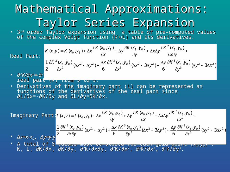
Mathematical Approximations: Mathematical Approximations: Taylor Series ExpansionTaylor Series Expansion

• 33rdrd order Taylor expansion using a table of pre-computed values of the order Taylor expansion using a table of pre-computed values of the complex Voigt function (K+complex Voigt function (K+ iiL) and its derivatives. L) and its derivatives.

Real Part:Real Part:

• ∂∂22K/∂xK/∂x22=-∂=-∂22K/∂yK/∂y22 decreases the number of stored derivatives of the real decreases the number of stored derivatives of the real part (K) from 9 to 6.part (K) from 9 to 6.

• Derivatives of the imaginary part (L) can be represented as functions of Derivatives of the imaginary part (L) can be represented as functions of the derivatives of the real part since the derivatives of the real part since ∂L/∂x=-∂K/∂y and ∂L/∂y=∂K/∂x.∂L/∂x=-∂K/∂y and ∂L/∂y=∂K/∂x.

Imaginary Part:Imaginary Part:

• ΔΔx=x-xx=x-x00, , ΔΔy=y-yy=y-y0 0 where (xwhere (x00,y,y00) is the closest gridpoint.) is the closest gridpoint.• A total of 8 values must be stored for each grid point (A total of 8 values must be stored for each grid point (xx00,,yy00) : K, L, ) : K, L, ∂K/∂x, ∂K/∂x,

∂K/∂y, ∂∂K/∂y, ∂22K/∂x∂y, ∂K/∂x∂y, ∂22K/∂xK/∂x22, ∂, ∂33K/∂xK/∂x33, ∂, ∂33K/∂yK/∂y33. .

)3(),(

6)3(

),(

6)(

),(

2

1

),(),(),(),(),(

223

003

223

003

222

002

002

000000

xyy

yxKyyx

x

yxKxyx

x

yxK

yx

yxKyx

y

yxKy

x

yxKxyxKyxK

)3(),(

6)3(

),(

6)(

),(

2

1

),(),(),(),(),(

223

003

223

003

22002

200

20000

00

xyx

yxKyyx

y

yxKxyx

yx

yxK

x

yxKyx

x

yxKy

y

yxKxyxLyxL

Mathematical Approximations:Mathematical Approximations:Lagrange Interpolating PolynomialsLagrange Interpolating Polynomials

• Used only in small areas when Used only in small areas when other methods fail, so does not other methods fail, so does not contribute significantly to contribute significantly to calculation time.calculation time.

• Employ equal grid point spacing Employ equal grid point spacing dxdx and and dy.dy.

• vv11, , vv22, , vv33 are the three grid points are the three grid points and and ∆v=(v- v∆v=(v- v22)/dv)/dv

• Four polynomial interpolations of Four polynomial interpolations of P(v) P(v) below are required for a spline below are required for a spline interpolation of real or imaginary interpolation of real or imaginary part.part.

• A total of eight evaluations is A total of eight evaluations is required for one complete function required for one complete function evaluation.evaluation.

n

j

n

jkk kj

kj vv

vvvPvP

1 ,1

)()(

))(2)()((2

1))()((

2

1)()( 213

2132 vPvPvPvvPvPvvPvP

* Note that the Lagrange interpolation regions along the x- and y- axes are * Note that the Lagrange interpolation regions along the x- and y- axes are so small that they barely appear on the graph.so small that they barely appear on the graph.

Programming TechniquesProgramming Techniques

• Calculates the Voigt profile for an entire spectral line Calculates the Voigt profile for an entire spectral line at one time, removing unnecessary subroutine calls.at one time, removing unnecessary subroutine calls.

• Each parameter involving y is calculated only once Each parameter involving y is calculated only once per spectral line, saving calculation time. per spectral line, saving calculation time.

• To do this we require equal spacing in wavenumber; To do this we require equal spacing in wavenumber; a version of the routine called for individual points is a version of the routine called for individual points is available, but not as time efficient. available, but not as time efficient.

• Interpolation tables stored as binary files on the hard Interpolation tables stored as binary files on the hard drive and read in only when needed. drive and read in only when needed.

• All files take up a total of 1.5 MB of memory, a small All files take up a total of 1.5 MB of memory, a small price to pay for the increase in accuracy and speed.price to pay for the increase in accuracy and speed.

Accuracy ComparisonsAccuracy Comparisons

Less than 10-6

Less than 10-4

↓↓

↑↑

J. Humlíček, J.Q.S.R.T., Vol. 27, 1982.J. Humlíček, J.Q.S.R.T., Vol. 27, 1982.

Maximum Error 7x10-4 Maximum Error 1.5x10-2

How bad do some routines get at small y?How bad do some routines get at small y?

Routines calculating only the Real PartRoutines calculating only the Real Part

R. J. Wells, J.Q.S.R.T., Vol. 62, R. J. Wells, J.Q.S.R.T., Vol. 62, 19991999

J. H. Pierluissi, J.Q.S.R.T., Vol. 18, 1977.J. H. Pierluissi, J.Q.S.R.T., Vol. 18, 1977.Twitty, Rarig, & Thompson, J.Q.S.R.T.,Vol. 24, 1980.Twitty, Rarig, & Thompson, J.Q.S.R.T.,Vol. 24, 1980.

S.R. Drayson, J.Q.S.R.T., Vol.16, 1976.S.R. Drayson, J.Q.S.R.T., Vol.16, 1976.

Speed ComparisonsSpeed Comparisons

Ratios of Calculation Times: Other routines to Benner & Letchworth

0

2

4

6

8

10

0<x<10,0<y<10

0<x<1000,0<y<1000

0<x<5,0<y<1

Drayson

Humlicek

Benner &Letchworth w/derivatives**

Humlíček

* Drayson calculates only the real part.* Drayson calculates only the real part.** These times are close to the final values, but the routine with** These times are close to the final values, but the routine withderivatives is still undergoing final testing.derivatives is still undergoing final testing.

*