Rank Co Occur

Frequency and Co-occurrence Analysis

Jamie CallanCarnegie Mellon University

[email protected]

95-779:Text Data Mining

© 2005, Jamie Callan2

Outline

• Finish Text Representation lecture• Frequency analysis

– Tokens and types– Type frequency tables– Zipf’s Law

• Brief overview of relational data mining– Co-occurrence of market basket items

• Associations between text features (co-occurrence)– Mutual Information Measure (MIM)– Phi-square (Φ2 )– Local context analysis (LCA)


Text Representation:Summary of Issues

Task: Convert the document into a set of featuresIssues: What makes a good feature?• Tokens: AT&T, drive-in, 527-4701, $1,110,427, …• Stopwords: Why remove stopwords? How are stopwords defined?• Stemming: Why stem? How do stemming algorithms work?• Phrases: Why index phrases? How are phrases recognized?


Feature Weights

• Okay, we think we know what makes a good text feature……how do we weight them?

• The state of the art is “tf.idf” indexing– tf stands for term frequency

» Words that occur a lot in a document represent its meaning well– idf stands for inverse document frequency

» Words that occur in many documents aren’t good at discriminating among documents


Feature Weights

• There are many tf formulas– Log (tf) + 1

» Doesn’t scale for document length– Log (tf) / Log (max_tf)

» Sensitive to small changes to lexical processing– tf / (tf + 0.5 + 1.5 * doclen / avg_doclen)

» One of the best– …

• There is more agreement about idf– Log (N / df) + 1– Log (( N / df) + 1) / (log (N) / 1)

» Scaled to [0..1]


Basic IR Concepts:Statistical Properties of Text

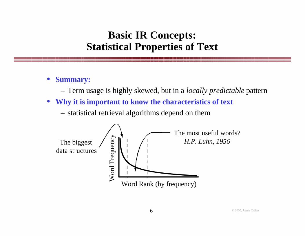
• Summary:– Term usage is highly skewed, but in a locally predictable pattern

• Why it is important to know the characteristics of text– statistical retrieval algorithms depend on them

Wor

d Fr

eque

ncy

Word Rank (by frequency)

The most useful words?H.P. Luhn, 1956The biggest

data structures


Text Representation:Summary

• Software doesn’t “understand” text– So, how do we map it into a form for use by computers?

• Convert the text to a set of tokens– Bag of words representation

• Lexical processing to produce features or index terms– Lexical processing, stopwords, stemming, phrases, …

• Statistical analysis to produce feature weights– Usually some form of tf.idf representation

• Maybe feature selection to discard unnecessary features• The result is a vector-space representation of text

– Also called a word histogram representation


Frequency Analysis:Introduction

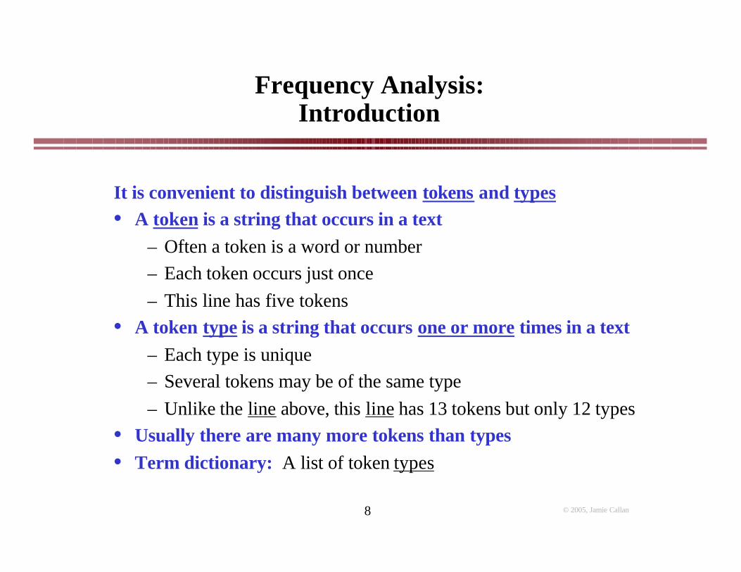
It is convenient to distinguish between tokens and types• A token is a string that occurs in a text

– Often a token is a word or number– Each token occurs just once– This line has five tokens

• A token type is a string that occurs one or more times in a text– Each type is unique– Several tokens may be of the same type– Unlike the line above, this line has 13 tokens but only 12 types

• Usually there are many more tokens than types• Term dictionary: A list of token types


Frequency Analysis:Initial Measures

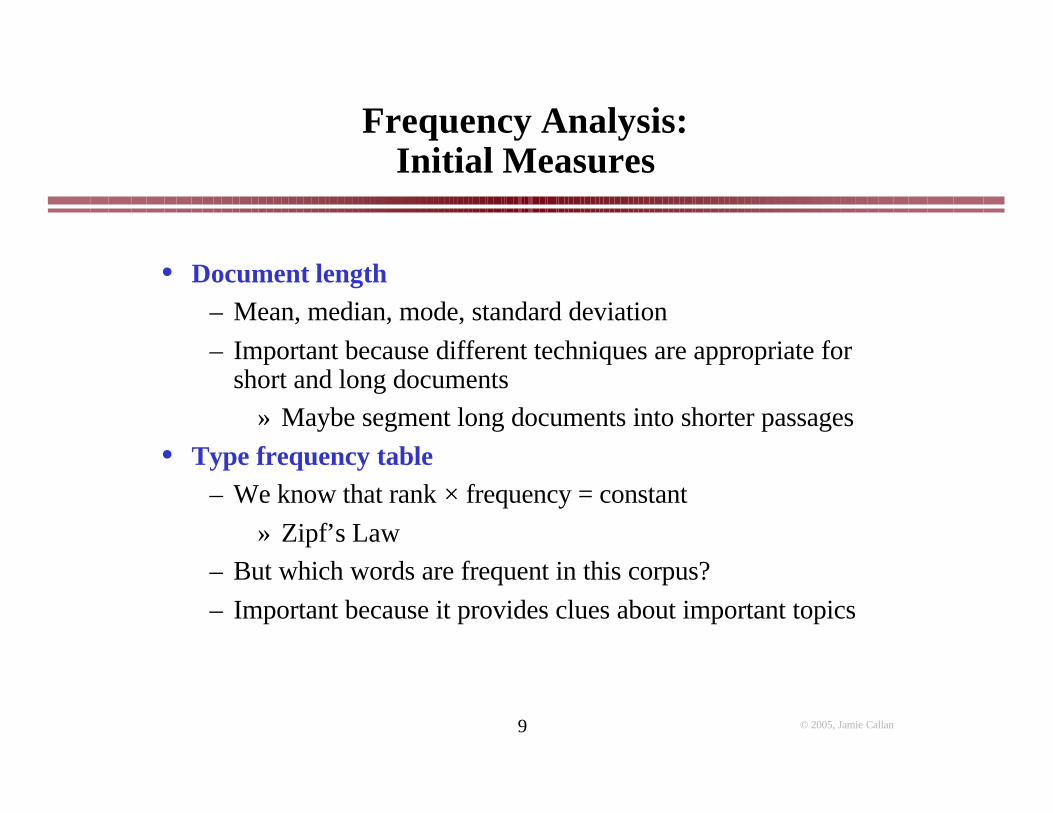
• Document length– Mean, median, mode, standard deviation– Important because different techniques are appropriate for

short and long documents» Maybe segment long documents into shorter passages

• Type frequency table– We know that rank × frequency = constant

» Zipf’s Law– But which words are frequent in this corpus?– Important because it provides clues about important topics


Frequency Analysis:Type Frequency Table

Type Frequency Type Frequencythe 1,130,021 by 118.863of 547,311 as 109,135to 516,635 at 101,779a 464,736 mr 101,679in 390,819 with 101,210and 387,703 from 96,900that 204,351 he 94,585for 199,340 million 93,515is 152,483 year 90,104said 148,302 its 86,774it 134,323 be 85,588on 121,173 was 83,398

WSJ87 collection (46,449 articles, 19 million tokens, 409 tokens/document, 132 MB)


Zipf’s “Law”

Zipf’s “Law” relates a term’s frequency to its rank• Rank the terms in a vocabulary by frequency, in descending order

• Empirical observation: PR = A/R A ≈ 0.1• Hence:• Rank x Frequency = Constant

– The constant ≈ N / 10 for English

f : Frequency of term ranked RR

N : Total number of word occurrences

NAfRRA

Nf

P RR

R =→==

∑ = == VR R

RR P

Nf

P 1 1


Zipf’s Law:Predicting Occurrence Frequencies

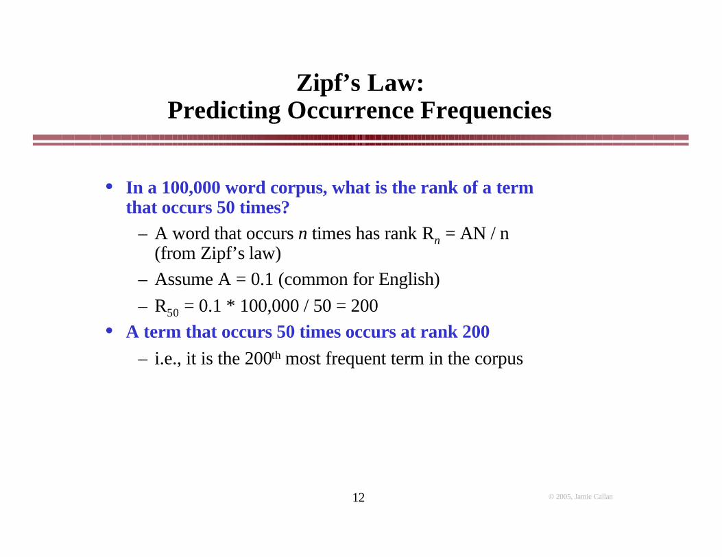
• In a 100,000 word corpus, what is the rank of a term that occurs 50 times?

– A word that occurs n times has rank Rn = AN / n(from Zipf’s law)

– Assume A = 0.1 (common for English)– R50 = 0.1 * 100,000 / 50 = 200

• A term that occurs 50 times occurs at rank 200– i.e., it is the 200th most frequent term in the corpus



• In a 100,000 word corpus, how many words occur 50 times?

– Several words may occur n times, rank them arbitrarily

– Assume rank Rn applies to last word that occurs n times

– Rn words occur at least n times – Rn+1 words occur at least n+1 times– The number of words that occur exactly n times is called In:

In = Rn – Rn+1 = AN/n – AN/(n+1) = AN/(n(n+1))– So, I50 = 0.1 * 100,000 / (50*51) = 3.9

• About 4 words occur exactly 50 times in a 100,000 word corpus

rank freq term: : :

r-1 n+1 wr n v: : :r n x

r+1 n-1 y: : :

Rn+1

Rn



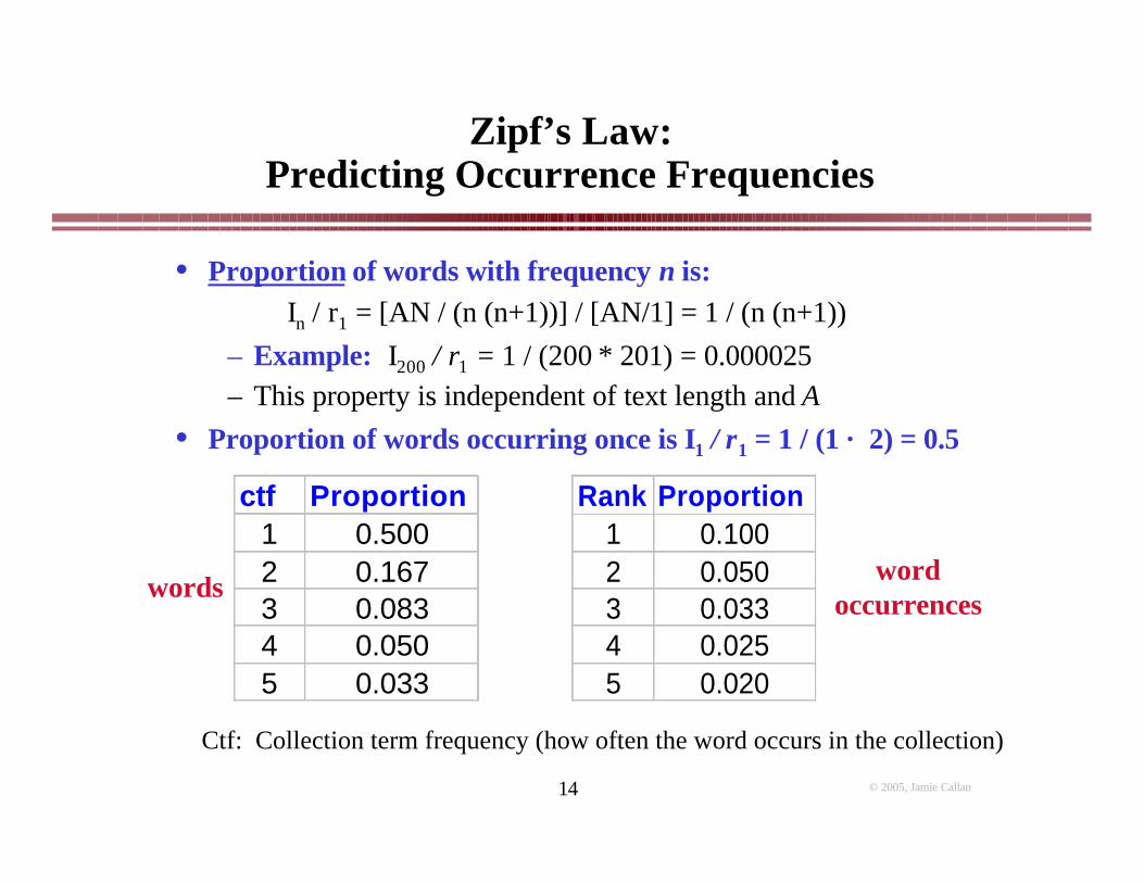
• Proportion of words with frequency n is: In / r1 = [AN / (n (n+1))] / [AN/1] = 1 / (n (n+1))

– Example: I200 / r1 = 1 / (200 ∗ 201) = 0.000025– This property is independent of text length and A

• Proportion of words occurring once is I1 / r1 = 1 / (1 × 2) = 0.5

ctf Proportion1 0.5002 0.1673 0.0834 0.0505 0.033

Rank Proportion1 0.1002 0.0503 0.0334 0.0255 0.020

words wordoccurrences

Ctf: Collection term frequency (how often the word occurs in the collection)



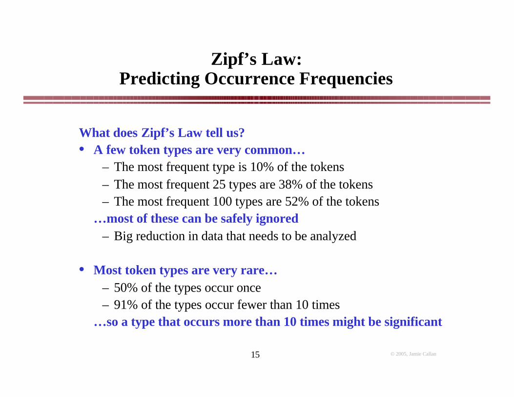
What does Zipf’s Law tell us?• A few token types are very common…

– The most frequent type is 10% of the tokens– The most frequent 25 types are 38% of the tokens– The most frequent 100 types are 52% of the tokens

…most of these can be safely ignored– Big reduction in data that needs to be analyzed

• Most token types are very rare…– 50% of the types occur once– 91% of the types occur fewer than 10 times

…so a type that occurs more than 10 times might be significant


Frequency Analysis

• Simple frequency analysis can be applied to anything– Tokens– Bigrams (two word sequences)– Noun sequences


Frequency Analysis Example

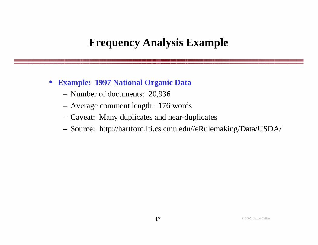
• Example: 1997 National Organic Data– Number of documents: 20,936– Average comment length: 176 words– Caveat: Many duplicates and near-duplicates– Source: http://hartford.lti.cs.cmu.edu//eRulemaking/Data/USDA/


Frequency Analysis:Bigrams

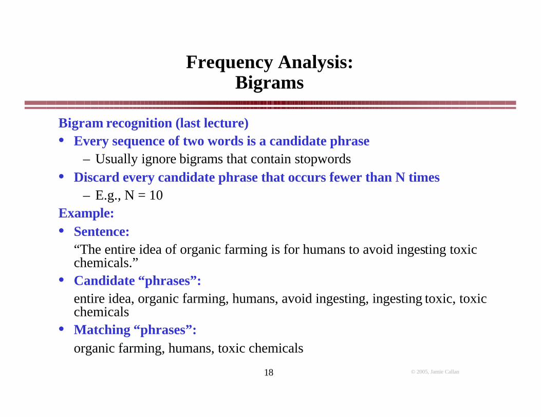
Bigram recognition (last lecture)• Every sequence of two words is a candidate phrase

– Usually ignore bigrams that contain stopwords• Discard every candidate phrase that occurs fewer than N times

– E.g., N = 10Example:• Sentence:

“The entire idea of organic farming is for humans to avoid ingesting toxic chemicals.”

• Candidate “phrases”:entire idea, organic farming, humans, avoid ingesting, ingesting toxic, toxic chemicals

• Matching “phrases”:organic farming, humans, toxic chemicals


Frequency Analysis:Bigrams

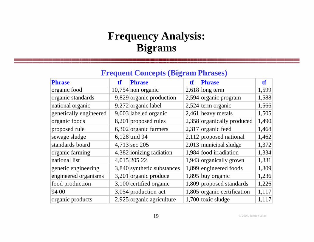
Frequent Concepts (Bigram Phrases)Phrase tf Phrase tf Phrase tforganic food 10,754 non organic 2,618 long term 1,599organic standards 9,829 organic production 2,594 organic program 1,588national organic 9,272 organic label 2,524 term organic 1,566genetically engineered 9,003 labeled organic 2,461 heavy metals 1,505organic foods 8,201 proposed rules 2,358 organically produced 1,490proposed rule 6,302 organic farmers 2,317 organic feed 1,468sewage sludge 6,128 tmd 94 2,112 proposed national 1,462standards board 4,713 sec 205 2,013 municipal sludge 1,372organic farming 4,382 ionizing radiation 1,984 food irradiation 1,334national list 4,015 205 22 1,943 organically grown 1,331genetic engineering 3,840 synthetic substances 1,899 engineered foods 1,309engineered organisms 3,201 organic produce 1,895 buy organic 1,236food production 3,100 certified organic 1,809 proposed standards 1,22694 00 3,054 production act 1,805 organic certification 1,117organic products 2,925 organic agriculture 1,700 toxic sludge 1,117


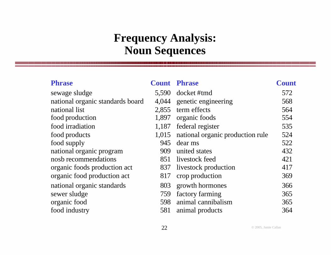
Frequency Analysis:Noun Sequences

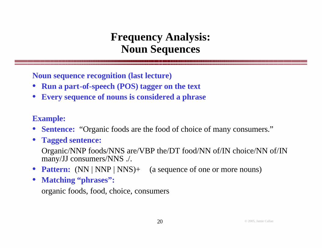
Noun sequence recognition (last lecture)• Run a part-of-speech (POS) tagger on the text• Every sequence of nouns is considered a phrase

Example:• Sentence: “Organic foods are the food of choice of many consumers.”• Tagged sentence:

Organic/NNP foods/NNS are/VBP the/DT food/NN of/IN choice/NN of/IN many/JJ consumers/NNS ./.

• Pattern: (NN | NNP | NNS)+ (a sequence of one or more nouns)• Matching “phrases”:

organic foods, food, choice, consumers



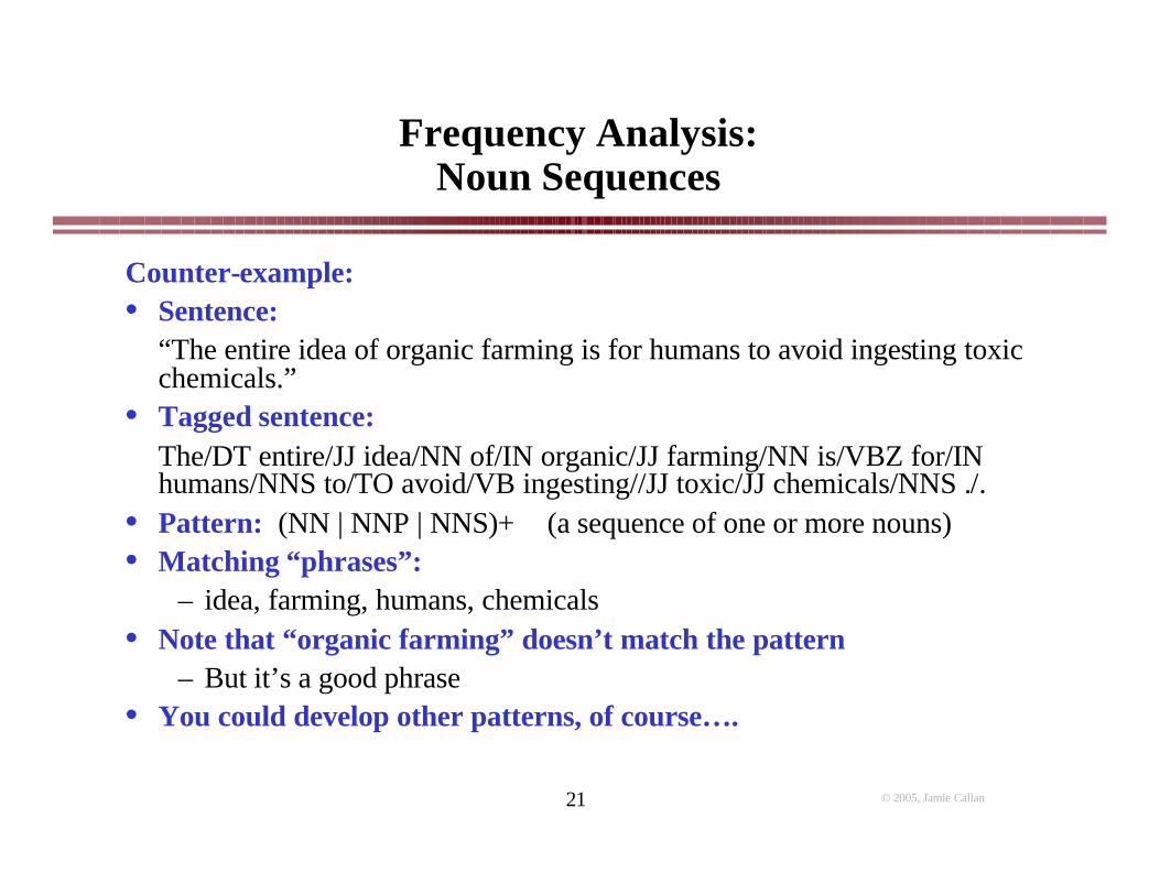
Counter-example:• Sentence:

“The entire idea of organic farming is for humans to avoid ingesting toxic chemicals.”

• Tagged sentence:The/DT entire/JJ idea/NN of/IN organic/JJ farming/NN is/VBZ for/IN humans/NNS to/TO avoid/VB ingesting//JJ toxic/JJ chemicals/NNS ./.

• Pattern: (NN | NNP | NNS)+ (a sequence of one or more nouns)• Matching “phrases”:

– idea, farming, humans, chemicals• Note that “organic farming” doesn’t match the pattern

– But it’s a good phrase• You could develop other patterns, of course….



364animal products581food industry365animal cannibalism598organic food365factory farming759sewer sludge366growth hormones803national organic standards369crop production817organic food production act417livestock production837organic foods production act421livestock feed851nosb recommendations432united states909national organic program522dear ms945food supply524national organic production rule1,015food products535federal register1,187food irradiation554organic foods1,897food production564term effects2,855national list568genetic engineering4,044national organic standards board572docket #tmd5,590sewage sludge

CountPhraseCountPhrase


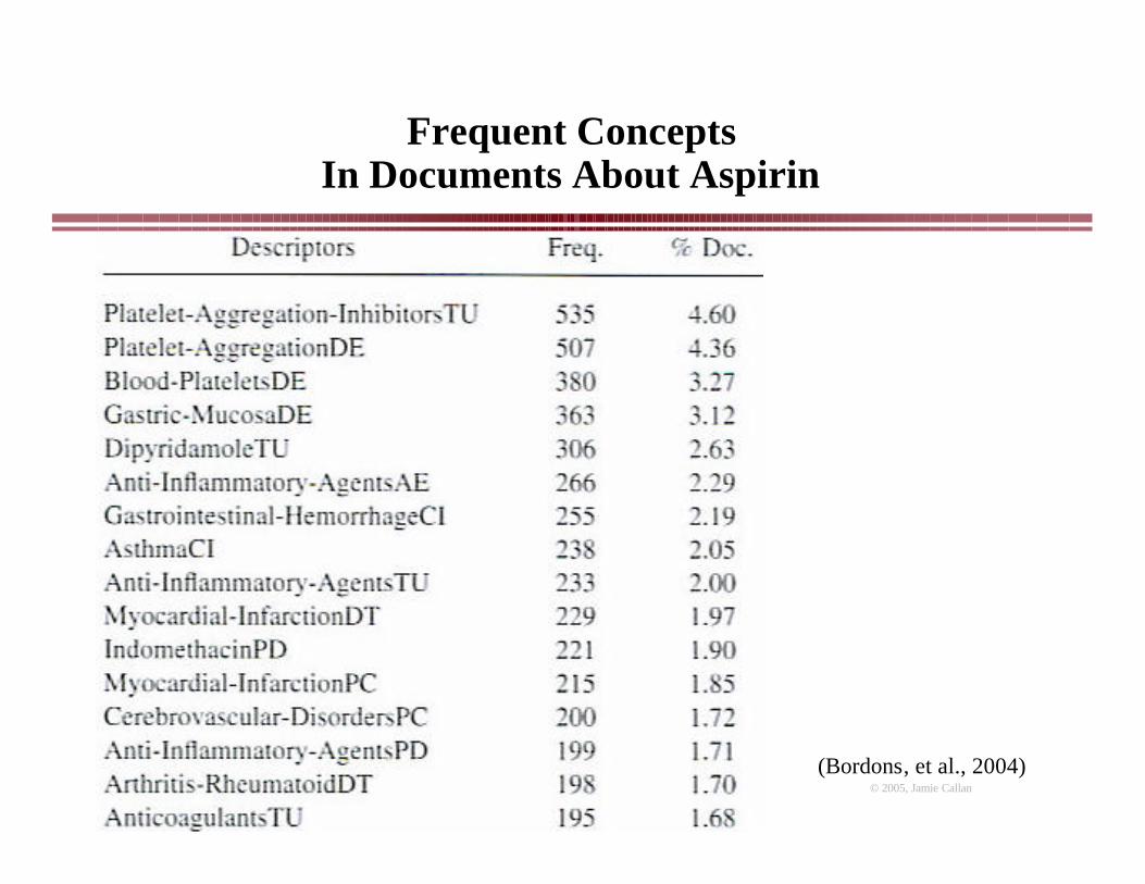
Frequent ConceptsIn Documents About Aspirin

(Bordons, et al., 2004)


Frequency Analysis:Summary

• Frequency analysis on simple types provides useful information– But, requires some data cleansing

» E.g., stopword removal• Frequency analysis on phrases can be more effective

– Stopwords are less of an issue– Phrase length is an issue for n-gram phrases– Noun phrases avoid having to pick a phrase length

» But miss other kinds of phrases» E.g., “genetically engineered”, “organic farming”


Introduction to Data Mining:General Overview

• A pattern is a model or structure identified in the data• Text mining is a process that searches for patterns that are:

– Valid for new data– Not known previously to the system (or, we hope, to us)– Potentially useful– Understandable

• Lessons learned from the field of Statistics– Patterns can be found even in data generated randomly

» They may even appear statistically significant• Patterns must be evaluated quantitatively

– E.g., estimated accuracy or utility


Introduction to Data Mining:Extra-Sensory Perception (ESP)

• David Rhine at Duke University in the 1950’s studied ESP– Students must guess which of 10 cards are red or black– About 1 in 1000 guess all 10 correct– Rhine concludes that about 1 in 1000 people have some ESP– When those students are retested later, they do about average

» “Telling people they have ESP causes them to lose it”– But…in a binary decision process, random guessing produces

a sequence of 10 correct choices about 1 / 210 times» 1 / 210 = 1 / 1024, or 1 out of 1000

• It is not hard to find patterns in data• It may be hard to find meaningful patterns in data

(Ullman)


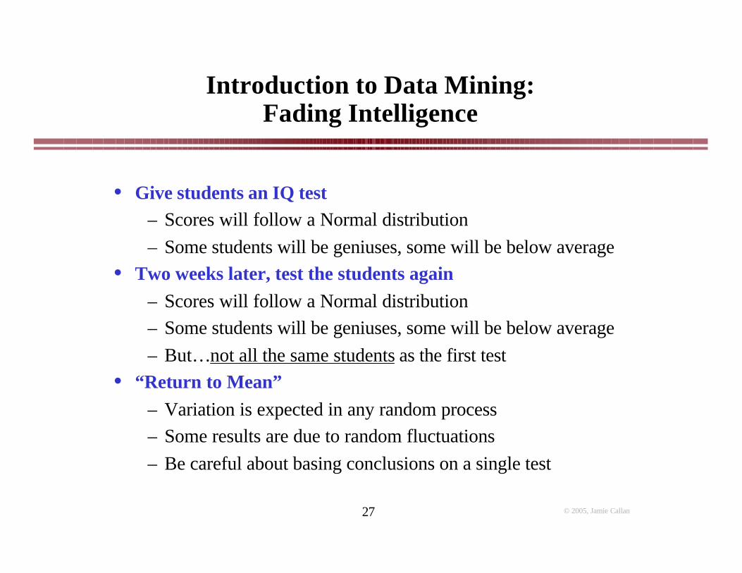
Introduction to Data Mining:Fading Intelligence

• Give students an IQ test– Scores will follow a Normal distribution– Some students will be geniuses, some will be below average

• Two weeks later, test the students again– Scores will follow a Normal distribution– Some students will be geniuses, some will be below average– But…not all the same students as the first test

• “Return to Mean”– Variation is expected in any random process– Some results are due to random fluctuations– Be careful about basing conclusions on a single test


Introduction to Data Mining

Data mining is a search for patterns supported by data• In principle, all patterns can be enumerated

– Usually a very large or infinite amount of time• Different algorithms are characterized by their search strategies

– What order they use to enumerate patterns– The size of the pattern space they search

» More expressive models à larger search space


Introduction to Data Mining

Before we start working with text……what do we know about data mining on relational data?


Market Basket Analysis:Association Rules (Link Analysis)

Suppose a store sells N different products and has data on B customer purchases (each purchase is called a “market basket”)

• An association rule is expressed as “If x is sold, then y is sold”– xày

• “Support” for x à y: Joint probability of P (x and y)– The probability of finding x and y together in a random basket

• “Confidence” in x à y: Conditional probability of P (y | x)– The probability of finding y in a basket if the basket already contains x

• Goal is rules with high support and high confidence– How are they computed?


Market Basket Analysis:Association Rules (Link Analysis)

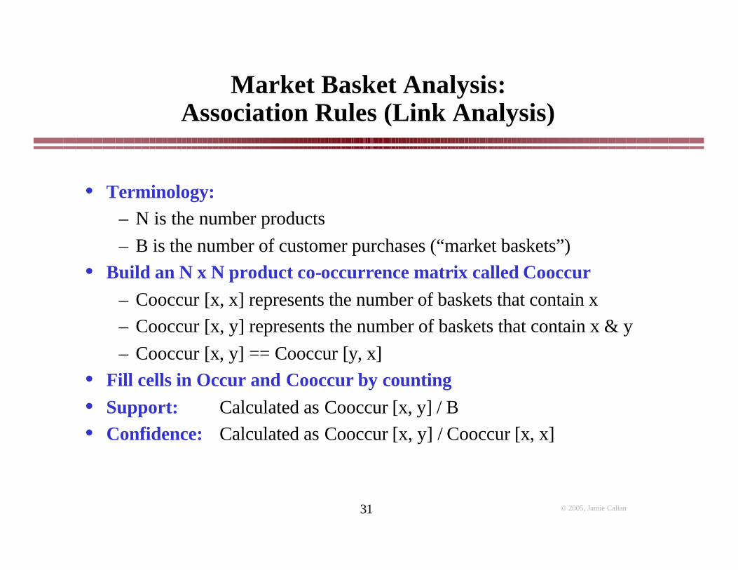
• Terminology:– N is the number products– B is the number of customer purchases (“market baskets”)

• Build an N x N product co-occurrence matrix called Cooccur– Cooccur [x, x] represents the number of baskets that contain x – Cooccur [x, y] represents the number of baskets that contain x & y– Cooccur [x, y] == Cooccur [y, x]

• Fill cells in Occur and Cooccur by counting• Support: Calculated as Cooccur [x, y] / B• Confidence: Calculated as Cooccur [x, y] / Cooccur [x, x]


Association Rules:Support and Confidence Example

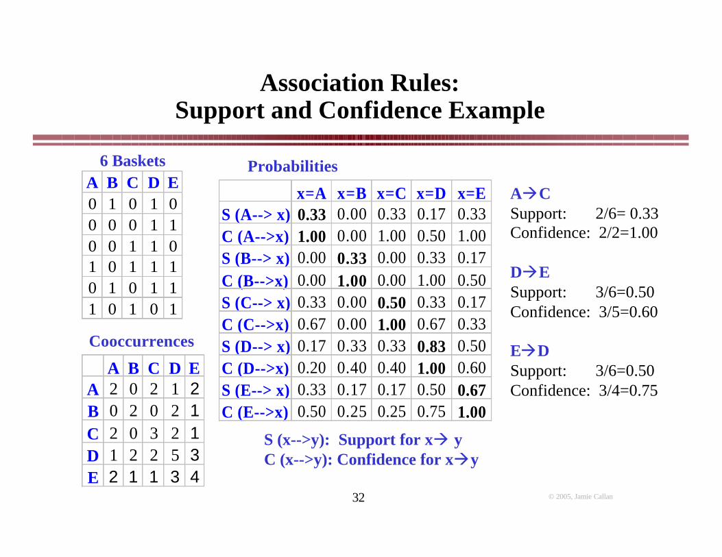
A B C D E0 1 0 1 00 0 0 1 10 0 1 1 01 0 1 1 10 1 0 1 11 0 1 0 1

6 Baskets

A B C D EA 2 0 2 1 2B 0 2 0 2 1C 2 0 3 2 1D 1 2 2 5 3E 2 1 1 3 4

Cooccurrences

x=A x=B x=C x=D x=ES (A--> x) 0.33 0.00 0.33 0.17 0.33C (A-->x) 1.00 0.00 1.00 0.50 1.00S (B--> x) 0.00 0.33 0.00 0.33 0.17C (B-->x) 0.00 1.00 0.00 1.00 0.50S (C--> x) 0.33 0.00 0.50 0.33 0.17C (C-->x) 0.67 0.00 1.00 0.67 0.33S (D--> x) 0.17 0.33 0.33 0.83 0.50C (D-->x) 0.20 0.40 0.40 1.00 0.60S (E--> x) 0.33 0.17 0.17 0.50 0.67C (E-->x) 0.50 0.25 0.25 0.75 1.00

Probabilities

AàCSupport: 2/6= 0.33Confidence: 2/2=1.00

DàESupport: 3/6=0.50Confidence: 3/5=0.60

EàDSupport: 3/6=0.50Confidence: 3/4=0.75

S (x-->y): Support for xà yC (x-->y): Confidence for xày


Market Basket Analysis:Association Rules

• Usually: C (yàx) > P (x)– If y is sold, it is more likely that x will be sold

• Sometimes: C (yàx) < P (x)– If y is sold, it is less likely that x will be sold

• “Lift” of rule “y à x” is C (yàx) / P (x)– If lift is 1.45, knowing that a customer bought y makes it 45%

more likely that she will buy x– If lift is 0.80, knowing that a customer bought y indicates only

an 80% probability that she will buy x– Lift (XàY) = Lift (YàX)

• Can be extended to any number of items• Usually look for rules that have high support, confidence and lift

– But, rules with low lift are interesting, too


Association Rules:Lift Example

A B C D E0 1 0 1 00 0 0 1 10 0 1 1 01 0 1 1 10 1 0 1 11 0 1 0 1

6 Baskets

A B C D EA 2 0 2 1 2B 0 2 0 2 1C 2 0 3 2 1D 1 2 2 5 3E 2 1 1 3 4

Cooccurrences

Probabilities

P(C) = 0.50DàCSupport: 2/6=0.33Confidence: 2/5=0.40Lift: 0.40 / 0.50 =0.80

P(A) = 0.33CàASupport: 2/6=0.33Confidence: 2/3=0.67Lift: 0.67 / 0.33=2.00

x=A x=B x=C x=D x=ES (A--> x) 0.33 0.00 0.33 0.17 0.33C (A-->x) 1.00 0.00 1.00 0.50 1.00S (B--> x) 0.00 0.33 0.00 0.33 0.17C (B-->x) 0.00 1.00 0.00 1.00 0.50S (C--> x) 0.33 0.00 0.50 0.33 0.17C (C-->x) 0.67 0.00 1.00 0.67 0.33S (D--> x) 0.17 0.33 0.33 0.83 0.50C (D-->x) 0.20 0.40 0.40 1.00 0.60S (E--> x) 0.33 0.17 0.17 0.50 0.67C (E-->x) 0.50 0.25 0.25 0.75 1.00

S (x-->y): Support for xà yC (x-->y): Confidence for xày


Text Mining and Association Rules

Can Association Rules be learned for text?• Yes, but…

– Different techniques and data structures would be used– Vocabulary > 100,000 for any reasonably large corpus– So an NxN matrix is usually not practical

• Could use a sparse matrix– Don’t store the zeros– Much more efficient

• Could use different features– E.g., noun phrases, named entities, …– Larger vocabulary, but each feature is less common


Co-Occurrence of Text Features

• Most search systems treat words as occurring independently– We know this is wrong

» E.g., “text” and “mining” are related• Co-occurrence measures attempt to identify things that tend

to occur together• There are many forms of co-occurrence

– E.g., phrasal: “text mining”, “make up”, “man and woman”– E.g., common associations: “Gates” and “Microsoft”

• An important part of text mining is finding co-occurrence relationships

– To create higher-level features, e.g., phrases– To identify important relationships


Collocation

• Co-occurrence patterns of words and word classes reveal significant information about how language is used

• Co-occurrence is based on text windows or discourse units– 5 word window approximates phrase co-occurrence– 20 word window approximates sentence co-occurrence– 100-200 word window approximates paragraph co-occurrence– Or….try to find phrases, sentences, paragraphs by other methods

• Co-occurrence patterns are used for:– Building dictionaries (lexicography)

» Including cross-lingual dictionaries– Building phrase dictionaries– Finding interesting relationships among concepts


Collocation and Linguistic Relations

Measure the average distance between words x and y within passages of text (e.g., paragraphs)

• Distance is location (y) – location (x)

Relation Word x Word y Separation Mean Variance Fixed Bread Butter 2.00 0.00 Drink Drive 2.00 0.00 Compound Computer Scientist 1.12 0.10 United States 0.98 0.14 Semantic Man Woman 1.46 8.07 Man Women -0.12 13.08 Lexical Refraining From 1.11 0.20 Coming From 0.83 2.89 Keeping From 2.14 5.53

1988 AP corpus (Church & Hanks)

“break and butter”“drink and drive”


Determining Collocations

• Simple frequency analysis identifies some interesting collocations– As in examples with the National Organic data

…but it doesn’t normalize for word frequency– A frequent term will have many frequent collocations

» E.g., “of the”, “in the”, “to the”, “on the”, “for the”• Simple frequency analysis is most effective

– After stopword removal– On features less likely to be affected by stopwords

» E.g., noun phrases, capitalized bigram phrases• For other features, more sophisticated measures are required


Determining Collocation

• Typical measure used is the point version of the mutual information measure

• Paired t test also used to compare collocation probabilities

• Chi-square and other tests are used, too

)p()p(),p(

log);I(yx

yxYX =

2

22

1

21 ss

x-xt

21

nn+

=


Measuring Co-Occurrenceof Text Features

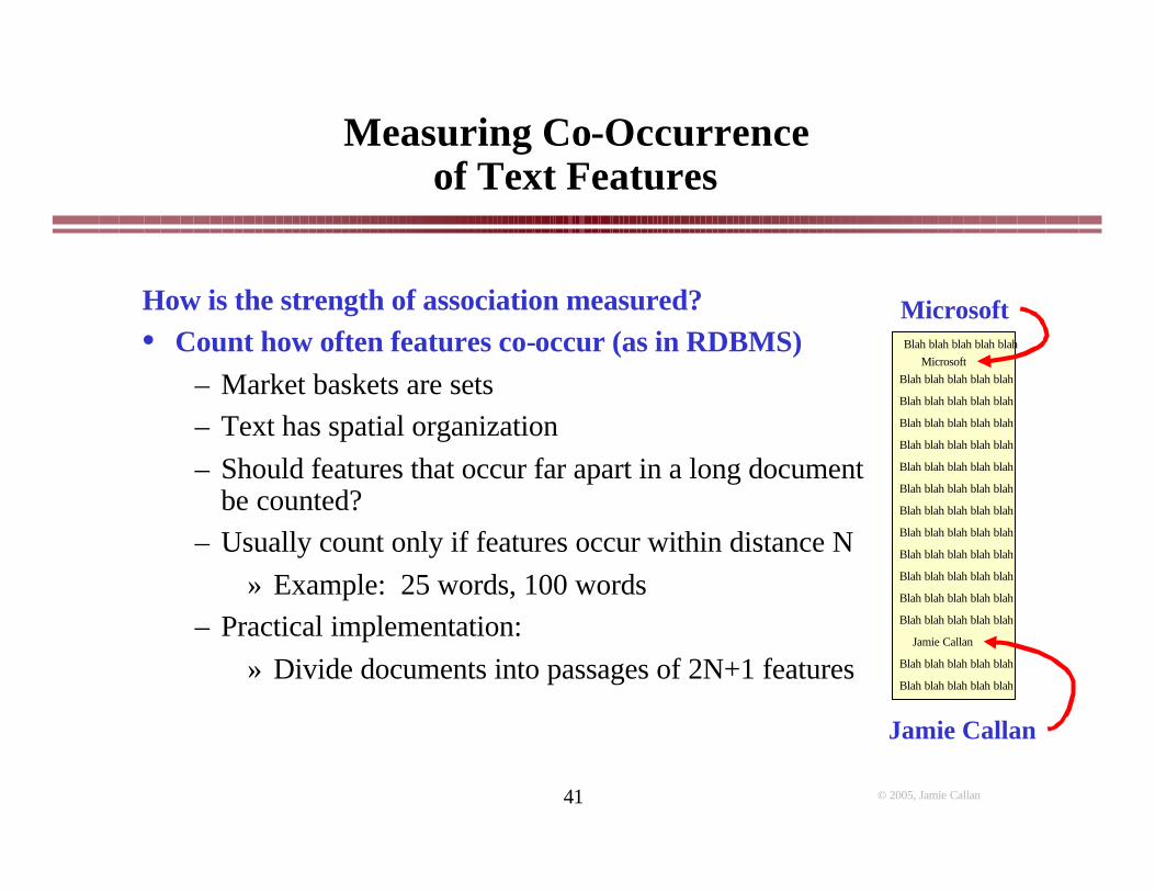
How is the strength of association measured?• Count how often features co-occur (as in RDBMS)

– Market baskets are sets– Text has spatial organization– Should features that occur far apart in a long document

be counted?– Usually count only if features occur within distance N

» Example: 25 words, 100 words– Practical implementation:

» Divide documents into passages of 2N+1 features

Microsoft

Jamie Callan

Microsoft

Jamie Callan

Blah blah blah blah blah
















Measuring Co-Occurrence Of Text Features:Mutual Information and Phi-Square

Microsoft

Jamie Callan

Microsoft

Bill Gates


Blah Bill Gates blah blah


Blah blah Microsoft

Bill Gates blah blah blah


Microsoft blah blah




Bill Gates blah blah blah





Win

dow

1W

indo

w 2

Win

dow

3

))()()(()(

Y)(X,

))(()(

logP(x)P(y)

y)P(x,logY)MIM(X,

22

22

dcdbcababcad

cabadcbaa

++++−

=

+++++

==

φ

Association Measures

Y YX a bX c d

ContingencyTable

• Count the number of windows containing X, Y, X&Y• Compute an association measure

– Mutual Information Measure (MIM)−∞ ≤ MIM (X,Y) ≤ ∞

– Phi-square (Φ2): favors high-frequency associations0 ≤ Φ2 (X, Y) ≤ 1

– Chi-square (χ2) = N * Φ2

• Differences between MIM and Φ2 difficult to evaluate– Φ2 may be slightly better


Collocation OverNamed Entity Representations

Example Wall Street Journal text:

Donald Trump Sells Hotel In New York to Australian

The developer Donald Trump said he sold the St. Moritz in Manhattan to Alan Bond, an Australian brewer and former America's Cup yachtsman, for $180 million.

Mr. Trump said he paid $31 million for the 700-room hotel in 1984. Real estate sources said the hotel has had a profit of roughly $12 million a year since then.

Mr. Trump said he decided to sell the St. Moritz because "I'm not looking to have two hotels on the same block.“ He recently acquired the Plaza Hotel, on the same street, for roughly $410 million.



[PER Donald Trump] [PER Sells Hotel] In [LOC New York] to [MISCAustralian]

The developer [PER Donald Trump] said he sold the [ORG St. Moritz] in [LOC Manhattan] to [PER Alan Bond] , an [MISC Australian] brewer and former [LOC America] 's [MISC Cup] yachtsman , for $ 180 million .

Mr. [PER Trump] said he paid $ 31 million for the 700-room hotel in 1984 . Real estate sources said the hotel has had a profit of roughly $ 12 million a year since then .

Mr. [PER Trump] said he decided to sell the [LOC St. Moritz] because " I'm not looking to have two hotels on the same block . " He recently acquired the [PER Plaza Hotel] , on the same street , for roughly $ 410 million .



• Note: Named-entity taggers make mistakes!– “Sells Hotel” is not a person– “America’s Cup” is an object, not a location + misc– Is “St. Moritz” a location or an organization?– “Plaza Hotel” is not a person

• We assume that errors are random and low-frequency– If something happens once, we don’t believe it very much– If it happens a lot, we believe it

» E.g., “Trump” is identified as a person several times



Document representation is a list of <NE type, NE string, location><PER, Donald Trump, 3><ORG, St. Moritz, 9><LOC, Manhattan, 12><PER, Alan Bond, 14><MISC, Australian, 17><LOC, America, 21><MISC, Cup, 22><PER, Trump, 28><PER, Trump, 59><LOC, St. Moritz, 66><PER, Plaza Hotel, 84>



Computing a contingency table:• Total passages: 173,252 • Donald Trump (X): 612

– So X = 173,252 – 612 = 172,640• St. Moritz (Y): 12

– So Y = 173,252 – 12 = 173,240• Donald Trump (X) & St. Moritz (Y): 3

Y YX 3 609 612X 9 172,631 172,640

12 173,240 173,252


Co-occurrence of People and Companies

Company Name CooccGolden Nugget 16Trump Castle Funding 4Hilton Hotels 13National Westminster 3First Fidelity Bancorp 10Merrill Lynch 2Pan Am 9American Express 5First Boston 2Citicorp 21

Company Name CooccMidlantic 10AMR 2Bankers 25UAL 2New York 9Shearson Lehman Brothers 3NWA 11Donaldson Lufkin & Jenrette 3Manufacturers Hanover 6Chase Manhattan 6

Query: Donald Trump

(Conrad & Utt, 1994)Φ2 measureCo-occurrences ≥ 2


Co-occurrence of People and Companies

Person Name CooccDennis Gomes 19Marjorie Everett 7Stephen A. Wynn 18Donald Trump 18Merv Griffen 2Randall D. Hubbard 3

Query: Golden Nugget

(Conrad & Utt, 1994)Φ2 measureCo-occurrences ≥ 2


For More Information

• M. Bordons, C. Bravo, and S. Barrigon. "Time-tracking of the research profile of a drug using bibliometric tools." JASIST, 55(5), Mar, 2004.

• J.G. Conrad and M.H. Utt. “A system for discovering relationships by feature extraction from text databases.” In SIGIR-94 conference proceedings. Available as publication IR-45 at http://ciir.cs.umass.edu/.

• J. Xu and W.B. Croft. “Query Expansion Using Local and Global Document Analysis.” SIGIR-96 conference proceedings. pp. 4-11. 1996.