vol. 177, no. 6 the american naturalist june 2011

Range Size Heritability in Carnivora Is Driven

by Geographic Constraints

Antonin Machac,1,2,* Jan Zrzavy,1 and David Storch2

1. Department of Zoology, Faculty of Science, University of South Bohemia, Branisovska 31, 370 05, Ceske Budejovice, Czech Republic;and Department of Statistics and Probability, University of Economics, nam. W. Churchilla 4, 130 67, Praha 3, Czech Republic; 2.Center for Theoretical Study, Charles University and Academy of Sciences of the Czech Republic, Jilska 1, 110 00, Praha 1, CzechRepublic; and Department of Ecology, Faculty of Sciences, Charles University, Vinicna 7, 128 44, Praha 2, Czech Republic

Submitted July 13, 2010; Accepted February 17, 2011; Electronically published May 3, 2011

Online enhancements: appendix. Dryad data: http://dx.doi.org/10.5061/dryad.8579.

abstract: Range size heritability refers to an intriguing patternwhere closely related species occupy geographic ranges of similarextent. Its existence may indicate selection on traits emergent onlyat the species level, with interesting consequences for evolutionaryprocesses. We explore whether range size heritability may be attrib-utable to the fact that range size is largely driven by the size ofgeographic domains (i.e., continents, biomes, areas given by species’climatic tolerance) that tend to be similar in phylogenetically relatedspecies. Using a well-resolved phylogeny of carnivorans, we showthat range sizes are indeed constrained by geographic domains andthat the phylogenetic signal in range sizes diminishes if the domainsizes are accounted for. Moreover, more detailed delimitation of spe-cies’ geographic domain leads to a weaker signal in range size her-itability, indicating the importance of definition of the null modelagainst which the pattern is tested. Our findings do not reject thehypothesis of range size heritability but rather unravel its underlyingmechanisms. Additional analyses imply that evolutionary conser-vatism in niche breadth delimits the species’ geographic domain,which in turn shapes the species’ range size. Range size heritabilitypatterns thus emerge as a consequence of this interplay betweenevolutionary and geographic constraints.

Keywords: macroecology, species selection, biogeography, eigenvec-tor, generalized least squares (GLS).

Introduction

During the last 2 decades, range size heritability has beena subject of vigorous and sometimes controversial debates.The term “range size heritability” refers to a tendency ofclosely related species to retain more similar range sizesthan distinct species do (Jablonski 1987). The appeal ofrange size heritability for biologists resides in its associa-tion with the species selection concept (Ricklefs and

* Corresponding author; e-mail: a.machac@email.cz.

Am. Nat. 2011. Vol. 177, pp. 767–779. � 2011 by The University of Chicago.

0003-0147/2011/17706-52305$15.00. All rights reserved.

DOI: 10.1086/659952

Latham 1992; Grantham 1995). Species selection is an out-come of heritable differences in speciation and extinctionrates among phylogenetic lineages. It is widely acceptedthat differential speciation and extinction owing to purelyemergent traits (collective properties of individuals withina species; e.g., geographic range size, sex ratio, intraspecificvariability) has to be due to the species selection. However,for any selection process, heritability of the selected traitsis a necessary prerequisite. Convincing evidence for rangesize heritability might therefore highlight the species se-lection as one of the central evolutionary processes (Gouldand Lloyd 1999; Webb and Gaston 2003; Jablonski 2008;Rabosky and McCune 2010).

Tempted by this outlook for crucial findings, numerousstudies have examined and variously documented (Ja-blonski 1987; Taylor and Gotelli 1994), refuted (Diniz-Filho and Torres 2002; Webb and Gaston 2003), and re-affirmed (Hunt et al. 2005; Jones et al. 2005) range sizeheritability via a spectrum of methods ranging from sister-species pair comparison and phylogenetic autocorrelationto the construction of explicit models of range size evo-lution (see reviews by Gaston 2003; Waldron 2007). Asrecent discussions illustrate (Hunt et al. 2005; Webb andGaston 2005), distinct methods may lead to different out-comes even when applied to the same data set. The am-biguous conclusions prove the range size heritability to bea difficult conundrum. This is not only due to the meth-odological pitfalls but also to presumably varied patternsamong different taxonomic groups (Jones et al. 2005).

Despite the lack of compelling evidence for the patternitself, many underlying mechanisms have been hypothe-sized and tested. For instance, phylogenetically conservedlife-history traits such as niche breadth, physiological tol-erance, dispersal ability, and functional group membershipmay eventually lead to range size heritability (Mouillotand Gaston 2009). Surprisingly, only rarely have geo-graphic constraints such as spatial limits of continents or

768 The American Naturalist

biomes been appraised (Bohning-Gaese et al. 2006; Freck-leton and Jetz 2009).

Spatial structure is an inherent component of biogeo-graphic data and is routinely considered when analyzingpatterns in diversity or abundance (Legendre et al. 2002;Blackburn 2004; Rangel et al. 2006). It naturally affectsrange sizes as well. As Brown et al. (1996, p. 607) high-lighted in their keystone work, we need to consider “howgeographic ranges are distributed on and constrained bythe spherical geometry and basic geography of the earth.”A number of studies have documented that species oc-cupying biogeographic provinces of vast spatial extent tendto have larger range sizes (Pagel et al. 1991; Smith et al.1994; Gaston et al. 1998; Fortes and Absalao 2004). Thismeans that we cannot make reliable conclusions aboutrange size heritability without controlling for spatiogeo-graphic constraints. However, only several studies so farhave addressed simultaneously the evolutionary and geo-graphic constituents of range sizes. Specifically, Freckletonand Jetz (2009) designed an integrated framework thatallowed simultaneous evaluation of phylogenetic and spa-tial components of life-history traits. Having detected spa-tial signal in range sizes, the authors outlined that rangesize variation may be driven by where species live ratherthan by evolutionary history. However, Bohning-Gaese etal. (2006) did not discover any substantial correlationwhen examining the relation between range sizes of 26bird species and the area of corresponding ecoregions andbiomes. These surprising conclusions are balanced by thefindings of Mouillot and Gaston (2009) that imply spatialautocorrelation in an extensive data set of 1,136 bird spe-cies (the autocorrelation is therein manifested as a positiverelationship between mutual overlap and similarity in sizeof sister species’ geographic ranges).

In our study, we thoroughly explore the impact of geo-graphic constraints on carnivoran range sizes. As delim-itation of specific geographic constraints might be con-tentious, we assess the constraints for several levels ofgeographic resolution (i.e., edges of continents, biomes,and climate envelopes). Subsequently, we contrast the ef-fects of geographic and phylogenetic constraints on rangesize variation. We evaluate the stability of phylogeneticsignal in range sizes after the correction for geographicconstraints, and explore possible causes of the revealedpatterns.

Material and Methods

We have employed a complex statistical approach to in-vestigate the effect of geographic constraints/domains onrange size heritability. Herein, we describe the foundationsof the methodological framework we adopted; a detailedtechnical description of the analyses and statistical pro-

cedures is given in appendix A in the online edition ofthe American Naturalist.

Overview

We assume that if range size is determined by the size ofa respective geographic domain, these two variables shouldcorrelate with each other. Moreover, if the range size her-itability (i.e., the phylogenetic signal in range size) is en-tirely due to the size of geographic domains, the residualsfrom the regression of range size on the domain size shouldhave no phylogenetic signal. This represents the first rel-atively simple approach to testing the effects of geographicdomains on range size.

For a detailed examination of the role of geographic andevolutionary constraints (i.e., the role of variously delim-ited geographic domains vs. the role of phylogeny), weperformed a decomposition of range size variation. How-ever, rather than exploring factors underlying species’range sizes, we explored factors responsible for range sizesimilarity. This means that we examined whether the sim-ilarity of species in terms of their range sizes is attributableto (a) species’ phylogenetic relatedness, (b) similarity inthe geographic location of species’ ranges, and (c) simi-larity of the size of species’ geographic domains (regardlessof physical distances between individual domains). Weproceeded using the following steps:

We constructed similarity matrices between all pairs ofspecies based on (a) patristic distances derived frombranch lengths of carnivoran phylogeny, (b) physical dis-tances between midpoints of species’ geographic ranges,and (c) differences between the areas of species’ geographicdomains (see below). Subsequently, we processed thesesimilarity matrices by means of the phylogenetic/spatialeigenvector filtering (or PVR1) and the phylogenetic/spa-tial generalized least squares (GLS).

The PVR procedure, based on metric multidimensionalscaling, transformed each of the distance matrices into aseries of mutually independent variables, forming either“phylogenetic filters” (Diniz-Filho and Torres 2002; Car-rascal et al. 2008) or “spatial filters” (Diniz-Filho and Bini2005). We regressed species’ actual range sizes against theset of spatial filters representing distances of range mid-points as well as the differences among the areas of eachspecies’ geographic domain. Subsequently, we explored theresiduals from these regressions for range size heritability,

1 Throughout the text, we use the abbreviation PVR to indicate eigenvector

filtering. The abbreviation itself stands for phylogenetic eigenvector regression

(termed “eigenvector filtering” by some authors). Since PVR is not restricted

to only phylogenetic applications and produces eigenvector filters, we feel that

the term “eigenvector filtering” is more appropriate for our purposes than

“phylogenetic eigenvector regression.” For brevity, however, we refer to ei-

genvector filtering by means of the widely known abbreviation PVR.

Exploring the Constraints on Range Sizes 769

that is, heritability after controlling for geographic posi-tion, and for the size of geographic domains. (In addition,see the appendix section “Eigenvector Filtering (PVR) andthe Generalized Least Squares (GLS) Framework” for adiscussion of the PVR inference and its drawbacks; Freck-leton et al. 2011.)

The GLS procedure, as proposed by Freckleton and Jetz(2009), modifies the method of phylogenetically indepen-dent contrasts to evaluate the phylogenetic and spatialcomponent of trait variance. To infer the role of spatialeffects (characterized by the distance matrices describedabove) with respect to range size, parameter F was esti-mated. Value of the F parameter ranges from 0 to 1. Azero value of F indicates that the range sizes are inde-pendent of the ranges’ spatial distances, whereas when

, the variation in species’ range sizes is attributableF p 1to space only.

Finally, the role of spatial and phylogenetic effects wascontrasted. In the case of the PVR, we performed variationpartitioning by means of a standard multiple regressionusing the sets of filters as independent variables and theactual range size as a dependent variable. We tested theeffect of individual variables (i.e., the sets of filters derivedfrom similarity/distance matrices), controlling for the re-maining effects, and also explored their common effect.This enabled us to evaluate the role of phylogeny whenaccounting for the effect of similarity in geographic do-main areas or similarity in range location, and vice versa.In the case of the GLS, we fitted an additional parameterl to the range size data simultaneously with F. The l

parameter transformed the variance-covariance matrix de-rived from the carnivoran phylogeny so that phylogenet-ically correlated variation as well as independent variationin range sizes was allowed for. Consequently, the relativeroles of spatial effects, phylogenetic effects, and effects in-dependent of both space and phylogeny could be assessed.Below, we provide details of all the calculations.

Geographic Ranges of Carnivora

Since carnivorans are among the most studied taxa inrange size heritability studies (Diniz-Filho and Torres 2002;Jones et al. 2005; Freckleton and Jetz 2009), we opted forthem as our model as well. Thus, our results will be com-parable with findings of the previous studies. Our data setcomprised 231 species of terrestrial carnivorans (i.e., ex-cluding Pinnipedia: Otariidae � Odobenidae � Phocidae).Maps of their geographic ranges were gathered from Pech-lakova (2006) and IUCN (2010). Whenever possible, theoriginal extent of ranges (i.e., not the extent recently re-duced by humans) was reconstructed. After digitalizationof the maps in ArcView GIS (ver. 3.2, Environmental Sys-

tems Research Institute, Redlands, CA), the range sizeswere calculated.

Assembling the Phylogeny

We constructed an updated phylogeny of carnivorans withparticular attention to recent studies (Bardeleben et al.2005; Lindblad-Toh et al. 2005; Fulton and Strobeck 2006;Gaubert and Cordeiro-Estrela 2006; Koepfli et al. 2006,2007; Arnason et al. 2007; Gaubert and Begg 2007; Krauseet al. 2008; Patou et al. 2009). To construct a supertree,the topology of partial phylogenies was coded using thematrix representation with parsimony method (Baum1992; Ragan 1992; for its phylogenetic applications see,e.g., Bininda-Emonds et al. 1999; Liu et al. 2001). Thephylogenetic data sets were analyzed by NONA software(ver. 2.0; Goloboff 1999).

We employed published information on dates of car-nivoran diversification events (Johnson et al. 2006; Koepfliet al. 2008; Patou et al. 2008; Sato et al. 2009; and studiescited above) to calibrate the branch lengths of our super-tree. Diversification estimates for nodes with no datingavailable were calculated in Phylocom v4.0 through theBLADJ algorithm, which minimizes the variance in branchlengths within the constraints of dated nodes, as describedin Webb et al. (2008).

Delimiting Geographic Constraints

Our baseline assumption stems from the obvious notionsthat every range size is restrained by the area of corre-sponding geographic domain (e.g., continent or biome;see below) and that range sizes within geographic domainsof similar sizes also tend to be similar. However, we needto address the fundamental question of how to define thegeographic domains. Since any particular definition wouldbe inevitably disputable as we do not know all the factorsshaping range sizes of individual species, we decided touse three different levels of spatial/geographic scale and tocontrast subsequent outcomes. For this reason we use threedistinct domain definitions (i.e., three levels of “geographicresolution”), differing in the amount of information usedfor the delimitation of domains: (a) continental domains,(b) biome domains, and (c) climate envelopes.

Continental geographic domains were represented bythe four distinct continents, that is, Africa, North andSouth America, and Eurasia. Island areas (British Isles,Borneo, Greenland, etc.) were affiliated with their adjacentcontinents.

Biome domains were represented by 14 biomes distin-guished by Olson et al. (2001). The area of individualbiomes was considered for each continent separately;within the continents, however, all the discrete areas of

770 The American Naturalist

individual biomes were merged. Each of the acquired areasrepresented a biome domain (e.g., all the temperate grass-lands of North America). If a species occurred in severalbiomes within a given continent, the total area of all bi-omes where the species occurred was taken as its biomedomain.

The most precise description of geographic domains wasacquired by means of climate envelopes (Guisan and Zim-mermann 2000). Climate envelopes were inferred for eachindividual species with respect to annual mean tempera-ture, annual precipitation, and NDVI (normalized differ-ence vegetation index, an estimate of environmental pro-ductivity based on spectral properties of vegetation) withinits geographic range. The original climate data sets (Hij-mans et al. 2005; Tucker et al. 2005) were resampled to a

-km spatial resolution, which is close to the rec-50 # 50ommended threshold of 1�–2� for species distribution data(Hurlbert and Jetz 2007). Climate envelope was delimitedas an area within which none of the above-mentionedenvironmental variables exceeded minimum or maximumvalues reached within the actual species’ range.

We need to explain what the climate envelopes representfrom the conceptual viewpoint. As Soberon and Nakamura(2009) illustrate, climate envelopes lie somewhere betweenthe species’ realized and fundamental niches. The enve-lopes do not incorporate biotic interactions (food webs,competition, etc.) and consider climate tolerances only.Thus, they approximate a species’ fundamental niche.However, the climate tolerances are inferred from species’geographic distributions which, ipso facto, represent therealized niche. Consequently, the area of a climate envelopeextends beyond the area of a species’ realized niche butdoes not reach the area corresponding to the fundamentalniche. Unlike more advanced techniques of niche mod-eling, the envelope-based approach is computationally ef-ficient and straightforward to interpret (Guisan andThuiller 2005). Its performance has been shown to beslightly worse but still satisfactory in comparison withmore sophisticated methods based on regression trees,multivariate distances, or maximum entropy (Kadmon etal. 2003; Elith et al. 2006).

Whenever the species occupied several isolated geo-graphic domains on different continents (e.g., America andEurasia in the case of Mustela erminea), the area of eachdomain was considered separately. We presume that thearea of isolated subranges is constrained by the corre-sponding domains independently and not by their sumacross different continents. Therefore, we handled theseisolated subranges as individual data points within ouranalyses. There were in fact only seven such cases in ourdata set (Canis lupus, Gulo gulo, Mustela erminea, Mustelanivalis, Panthera pardus, Ursus arctos, Vulpes vulpes).

We need to explicitly notify the readers that information

on geographic domains was inferred from the species’ geo-graphic ranges. As a consequence, the more informationinferred from the species’ geographic distribution we usedfor a delimitation of its domain, the closer the domainwas to the species’ actual geographic range. Consideringthis inevitable circularity associated with domain defini-tion, we a priori expect the effect of geographic domainson range size to increase with the geographic resolution(continents, biomes, climate envelopes) at which the do-main was defined.

Constructing Similarity Matrices

We prepared three matrices of similarity between species’ranges: (1) matrix of phylogenetic distances between spe-cies, (2) matrix of distances between locations of speciesranges, and (3) matrix of differences in areas of geographicdomains, which were delimited as explained above.

Phylogenetic relatedness was represented by patristicdistances among individual species. The distances werederived from the branch lengths of our carnivoran phy-logeny (see above).

To create a distance matrix of range locations, we com-puted mutual physical distances among range midpoints(i.e., the average from maximum and minimum rangeextents in east-west and north-south directions). Thismeasure was employed by previous studies (Freckleton andJetz 2009) and allows us to compare the obtained results.

The distances between areas of species’ geographic do-mains were calculated in two ways. Both of the distancesincrease with the dissimilarity of geographic domains’ ar-eas, regardless of ranges’ mutual physical distance:

S(B)distance 1 (A, B) p log , (1)

S(A)

distance 2 (A, B) p log [S(B) � S(A)], (2)

where distance (A, B) is the distance between ranges Aand B, and S(A), S(B) are areas of geographic domainsfor species A and B, respectively, so that . WeS(A) ! S(B)calculated the distances distance 1 and distance 2 for eachof the three geographic resolutions (i.e., continents, bi-omes, and climate envelopes). Subsequently, the distancematrices were processed by the PVR and the GLS (as de-scribed above and in “Eigenvector Filtering (PVR) and theGeneralized Least Squares (GLS) Framework”).

Assessing Range Size Heritability

The range size heritability was assessed by means of Blom-berg’s K (Blomberg et al. 2003), Pagel’s l (Freckleton etal. 2002), and Moran’s I (Gittleman and Kot 1990; Le-gendre et al. 2002; Jones et al. 2005). We favor Moran’s I

Exploring the Constraints on Range Sizes 771

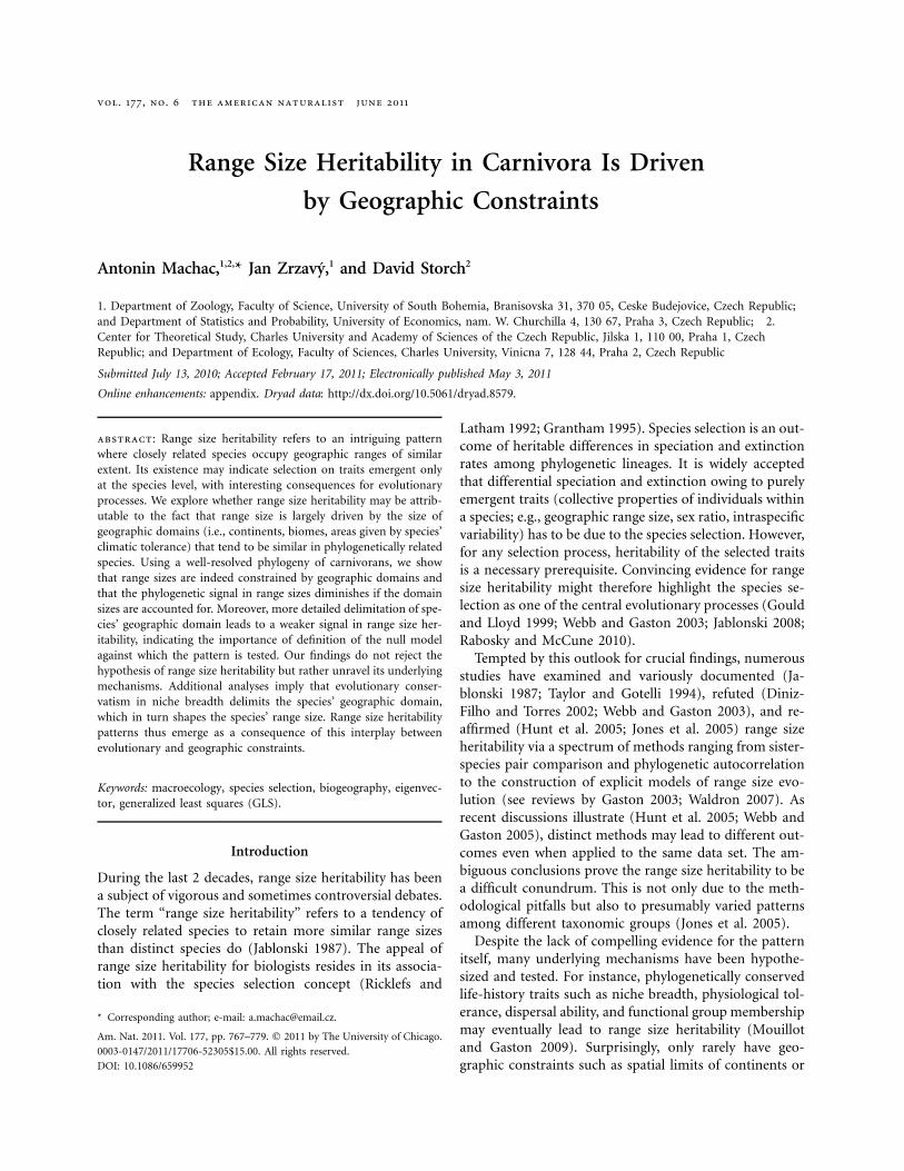
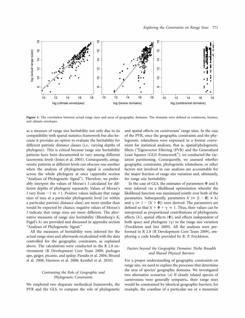
Figure 1: The correlation between actual range sizes and areas of geographic domains. The domains were defined as continents, biomes,and climate envelopes.

as a measure of range size heritability not only due to itscompatibility with spatial statistics framework but also be-cause it provides an option to evaluate the heritability fordifferent patristic distance classes (i.e., varying depths ofphylogeny). This is critical because range size heritabilitypatterns have been documented to vary among differenttaxonomic levels (Jones et al. 2005). Consequently, antag-onistic patterns at different levels can obscure one anotherwhen the analysis of phylogenetic signal is conductedacross the whole phylogeny at once (appendix section“Analyses of Phylogenetic Signal”). Therefore, we prefer-ably interpret the values of Moran’s I calculated for dif-ferent depths of phylogeny separately. Values of Moran’sI vary from �1 to �1. Positive values indicate that rangesizes of taxa at a particular phylogenetic level (or withina particular patristic distance class) are more similar thanwould be expected by chance; negative values of Moran’sI indicate that range sizes are more different. The alter-native measures of range size heritability (Blomberg’s K,Pagel’s l) are provided and discussed in appendix section“Analyses of Phylogenetic Signal.”

All the measures of heritability were inferred for theactual range sizes and afterwards recalculated with the datacontrolled for the geographic constraints, as explainedabove. The calculations were conducted in the R 2.8 en-vironment (R Development Core Team 2009; packagesape, geiger, picante, and spdep; Paradis et al. 2004; Bivandet al. 2008; Harmon et al. 2008; Kembel et al. 2010).

Contrasting the Role of Geographic andPhylogenetic Constraints

We employed two disparate methodical frameworks, thePVR and the GLS, to compare the role of phylogenetic

and spatial effects on carnivorans’ range sizes. In the caseof the PVR, once the geographic constraints and the phy-logenetic relatedness were expressed in a format conve-nient for statistical analyses, that is, spatial/phylogeneticfilters (“Eigenvector Filtering (PVR) and the GeneralizedLeast Squares (GLS) Framework”), we conducted the var-iation partitioning. Consequently, we assessed whethergeographic constraints, phylogenetic relatedness, or otherfactors not involved in our analyses are accountable forthe major fraction of range size variation and, ultimately,for range size heritability.

In the case of GLS, the estimates of parameters F and l

were inferred via a likelihood optimization whereby thelikelihood function was maximized jointly over both of theparameters. Subsequently, parameters ′l (p [1 � F] # l)and were derived. The parameters are′g (p 1 � [l � F])defined so that . Thus, their values can be′l � F � g p 1interpreted as proportional contributions of phylogeneticeffects (l′), spatial effects (F), and effects independent ofboth space and phylogeny (g) to the range size variation(Freckleton and Jetz 2009). All the analyses were per-formed in R 2.8 (R Development Core Team 2009), em-ploying a code kindly provided by R. P. Freckleton.

Factors beyond the Geographic Domains: Niche Breadthand Shared Physical Barriers

For a proper understanding of geographic constraints onrange size, we need to explore the processes that determinethe area of species’ geographic domains. We investigatedtwo alternative scenarios: (a) If closely related species ofcarnivorans were generally sympatric, their range sizeswould be constrained by identical geographic barriers; forexample, the coastline of a particular sea or a mountain

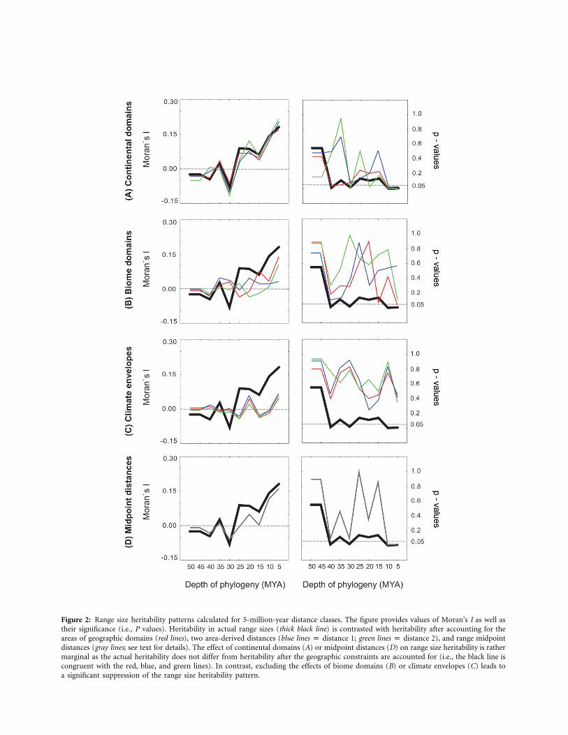
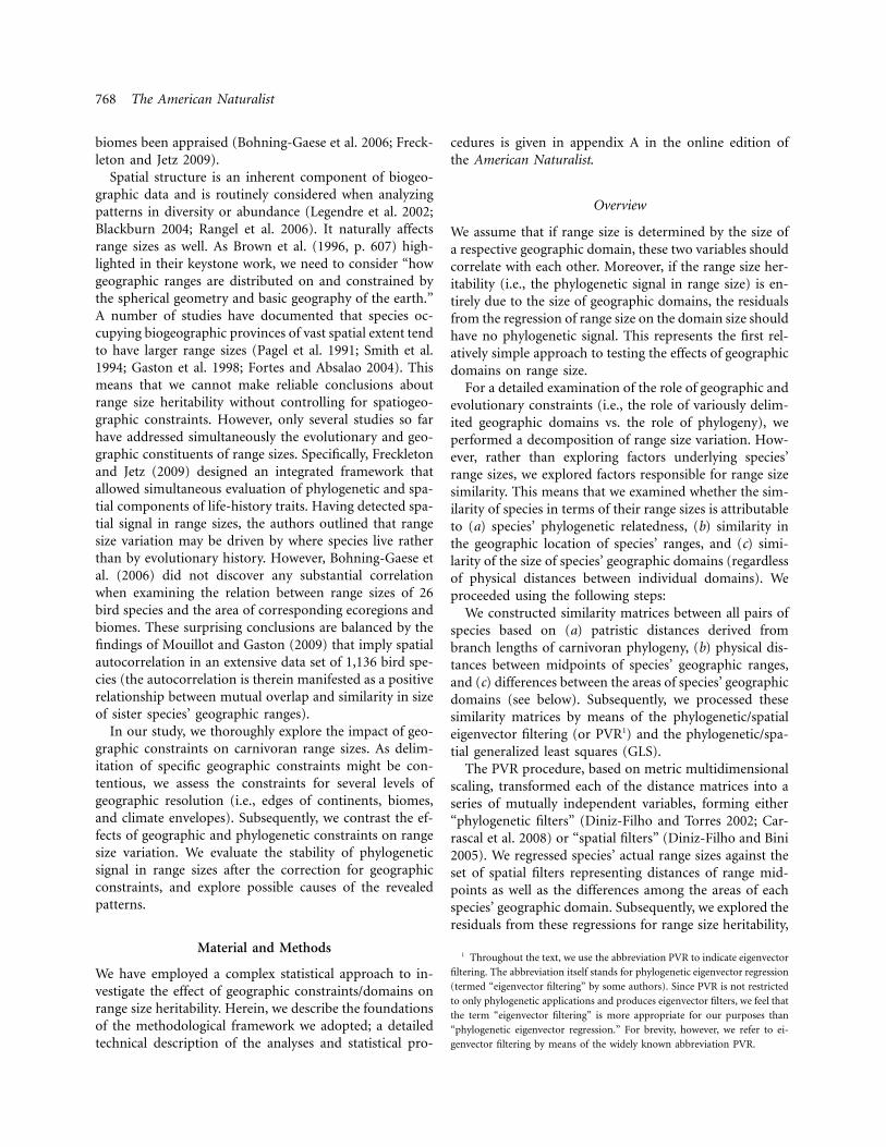
Figure 2: Range size heritability patterns calculated for 5-million-year distance classes. The figure provides values of Moran’s I as well astheir significance (i.e., P values). Heritability in actual range sizes (thick black line) is contrasted with heritability after accounting for theareas of geographic domains (red lines), two area-derived distances (blue lines p distance 1; green lines p distance 2), and range midpointdistances (gray lines; see text for details). The effect of continental domains (A) or midpoint distances (D) on range size heritability is rathermarginal as the actual heritability does not differ from heritability after the geographic constraints are accounted for (i.e., the black line iscongruent with the red, blue, and green lines). In contrast, excluding the effects of biome domains (B) or climate envelopes (C) leads toa significant suppression of the range size heritability pattern.

Exploring the Constraints on Range Sizes 773

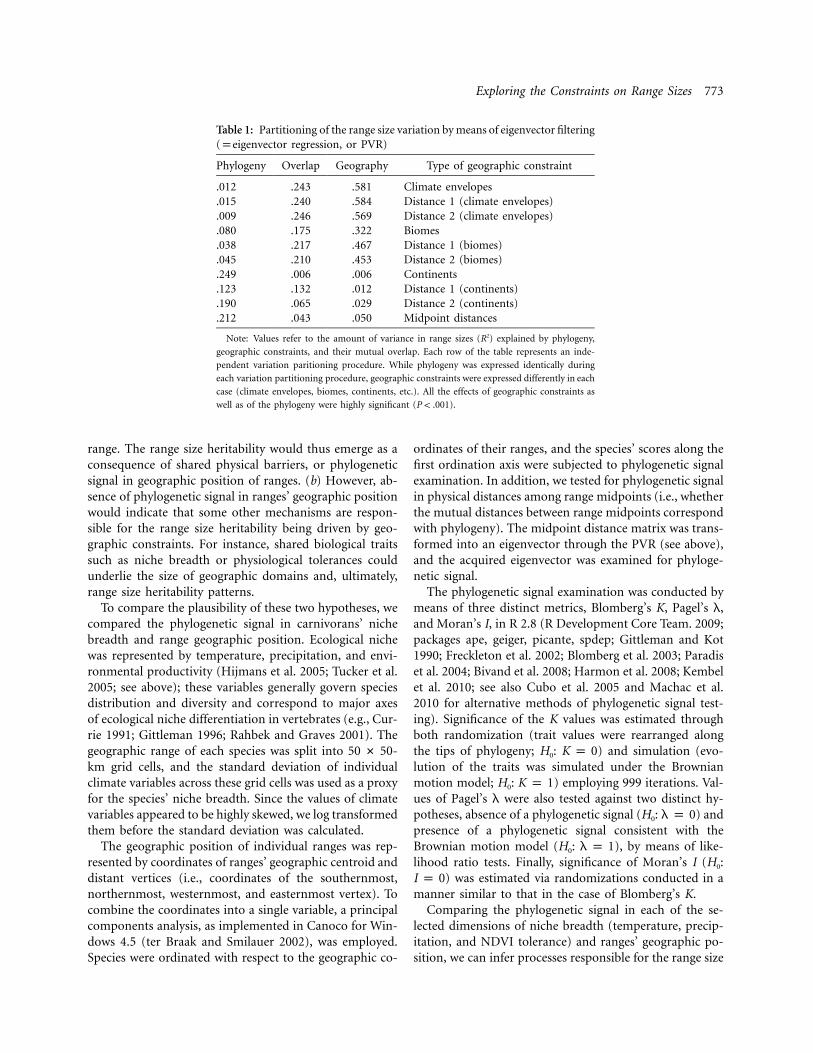
Table 1: Partitioning of the range size variation by means of eigenvector filtering(peigenvector regression, or PVR)

Phylogeny Overlap Geography Type of geographic constraint

.012 .243 .581 Climate envelopes

.015 .240 .584 Distance 1 (climate envelopes)

.009 .246 .569 Distance 2 (climate envelopes)

.080 .175 .322 Biomes

.038 .217 .467 Distance 1 (biomes)

.045 .210 .453 Distance 2 (biomes)

.249 .006 .006 Continents

.123 .132 .012 Distance 1 (continents)

.190 .065 .029 Distance 2 (continents)

.212 .043 .050 Midpoint distances

Note: Values refer to the amount of variance in range sizes (R2) explained by phylogeny,

geographic constraints, and their mutual overlap. Each row of the table represents an inde-

pendent variation paritioning procedure. While phylogeny was expressed identically during

each variation partitioning procedure, geographic constraints were expressed differently in each

case (climate envelopes, biomes, continents, etc.). All the effects of geographic constraints as

well as of the phylogeny were highly significant ( ).P ! .001

range. The range size heritability would thus emerge as aconsequence of shared physical barriers, or phylogeneticsignal in geographic position of ranges. (b) However, ab-sence of phylogenetic signal in ranges’ geographic positionwould indicate that some other mechanisms are respon-sible for the range size heritability being driven by geo-graphic constraints. For instance, shared biological traitssuch as niche breadth or physiological tolerances couldunderlie the size of geographic domains and, ultimately,range size heritability patterns.

To compare the plausibility of these two hypotheses, wecompared the phylogenetic signal in carnivorans’ nichebreadth and range geographic position. Ecological nichewas represented by temperature, precipitation, and envi-ronmental productivity (Hijmans et al. 2005; Tucker et al.2005; see above); these variables generally govern speciesdistribution and diversity and correspond to major axesof ecological niche differentiation in vertebrates (e.g., Cur-rie 1991; Gittleman 1996; Rahbek and Graves 2001). Thegeographic range of each species was split into -50 # 50km grid cells, and the standard deviation of individualclimate variables across these grid cells was used as a proxyfor the species’ niche breadth. Since the values of climatevariables appeared to be highly skewed, we log transformedthem before the standard deviation was calculated.

The geographic position of individual ranges was rep-resented by coordinates of ranges’ geographic centroid anddistant vertices (i.e., coordinates of the southernmost,northernmost, westernmost, and easternmost vertex). Tocombine the coordinates into a single variable, a principalcomponents analysis, as implemented in Canoco for Win-dows 4.5 (ter Braak and Smilauer 2002), was employed.Species were ordinated with respect to the geographic co-

ordinates of their ranges, and the species’ scores along thefirst ordination axis were subjected to phylogenetic signalexamination. In addition, we tested for phylogenetic signalin physical distances among range midpoints (i.e., whetherthe mutual distances between range midpoints correspondwith phylogeny). The midpoint distance matrix was trans-formed into an eigenvector through the PVR (see above),and the acquired eigenvector was examined for phyloge-netic signal.

The phylogenetic signal examination was conducted bymeans of three distinct metrics, Blomberg’s K, Pagel’s l,and Moran’s I, in R 2.8 (R Development Core Team. 2009;packages ape, geiger, picante, spdep; Gittleman and Kot1990; Freckleton et al. 2002; Blomberg et al. 2003; Paradiset al. 2004; Bivand et al. 2008; Harmon et al. 2008; Kembelet al. 2010; see also Cubo et al. 2005 and Machac et al.2010 for alternative methods of phylogenetic signal test-ing). Significance of the K values was estimated throughboth randomization (trait values were rearranged alongthe tips of phylogeny; H0: ) and simulation (evo-K p 0lution of the traits was simulated under the Brownianmotion model; H0: ) employing 999 iterations. Val-K p 1ues of Pagel’s l were also tested against two distinct hy-potheses, absence of a phylogenetic signal (H0: ) andl p 0presence of a phylogenetic signal consistent with theBrownian motion model (H0: ), by means of like-l p 1lihood ratio tests. Finally, significance of Moran’s I (H0:

) was estimated via randomizations conducted in aI p 0manner similar to that in the case of Blomberg’s K.

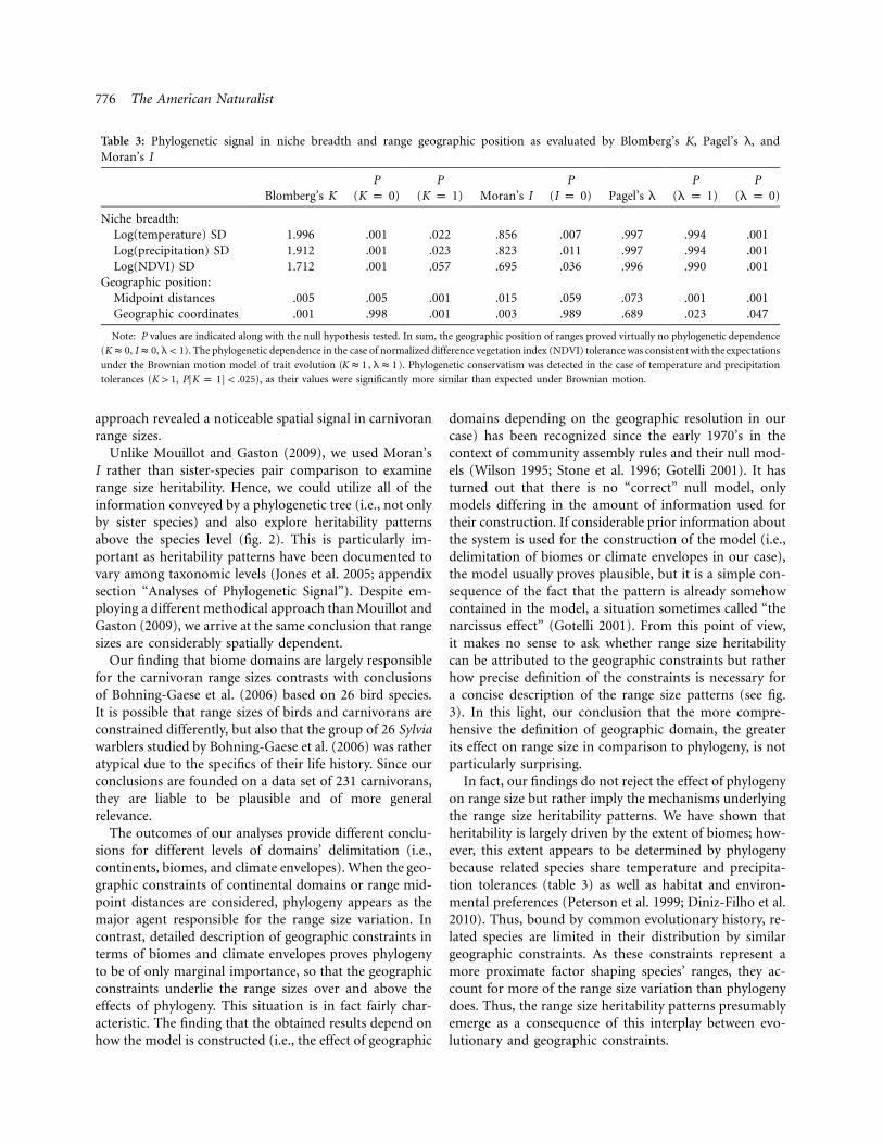
Comparing the phylogenetic signal in each of the se-lected dimensions of niche breadth (temperature, precip-itation, and NDVI tolerance) and ranges’ geographic po-sition, we can infer processes responsible for the range size

774 The American Naturalist

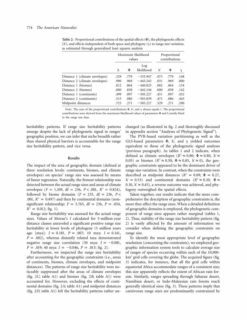
Table 2: Proportional contributions of the spatial effects (F), the phylogenetic effects(l′), and effects independent of both space and phylogeny (g) to range size variation,as estimated through generalized least squares analysis

Maximum likelihoodvalues

Proportionalcontributions

l F

Loglikelihood l′ F g

Distance 1 (climate envelopes) .329 .779 �335.947 .073 .779 .148Distance 2 (climate envelopes) .990 .969 �443.243 .031 .969 .000Distance 1 (biomes) .012 .864 �440.025 .002 .864 .134Distance 2 (biomes) .000 .858 �442.144 .000 .858 .142Distance 1 (continents) .499 .097 �505.227 .451 .097 .452Distance 2 (continents) .515 .086 �503.839 .471 .086 .443Midpoint distances .725 .271 �505.227 .529 .271 .200

Note: The sum of the proportional contributions F, l′, and g always equals 1. The proportional

contributions were derived from the maximum likelihood values of parameters F and l jointly fitted

to the range size data.

heritability patterns. If range size heritability patternsemerge despite the lack of phylogenetic signal in ranges’geographic position, we can infer that niche breadth ratherthan shared physical barriers is accountable for the rangesize heritability pattern, and vice versa.

Results

The impact of the area of geographic domain (defined atthree resolution levels: continents, biomes, and climateenvelopes) on species’ range size was assessed by meansof linear regression. Naturally, the firmest relationship wasdetected between the actual range sizes and areas of climateenvelopes ( , , , ),2F p 1,109 df p 236 P ! .001 R p 0.824followed by biome domains ( , ,F p 235 df p 236 P !

, ) and then by continental domains (non-2.001 R p 0.497significant relationship: , , ,F p 3.765 df p 236 P p .054

; fig. 1).2R p 0.012Range size heritability was assessed for the actual range

sizes. Values of Moran’s I calculated for 5-million-yeardistance classes unraveled a significant positive range sizeheritability at lower levels of phylogeny (5 million yearsago [mya]: , ; 10 mya: ,I p 0.181 P p .007 I p 0.141

), whereas distantly related taxa demonstratedP p .002negative range size correlation (30 mya: ,I p �0.081

; 40 mya: , ; fig. 2).P p .019 I p �0.046 P p .013Furthermore, we inspected the range size heritability

after accounting for the geographic constraints (i.e., areasof continents, biomes, climate envelopes, and midpointdistances). The patterns of range size heritability were no-ticeably suppressed after the areas of climate envelopes(fig. 2C; table A1) and biomes (fig. 2B; table A1) wereaccounted for. However, excluding the effects of conti-nental domains (fig. 2A; table A1) and midpoint distances(fig. 2D; table A1) left the heritability patterns rather un-

changed (as illustrated in fig. 2 and thoroughly discussedin appendix section “Analyses of Phylogenetic Signal”).

The PVR-based variation partitioning as well as theGLS-based parameters F, l′, and g yielded outcomesequivalent to those of the phylogenetic signal analyses(previous paragraph). As tables 1 and 2 indicate, whendefined as climate envelopes ( ; ,2 ′R ≈ 0.80 F ≈ 0.80 l ≈

) or biomes ( ; , ), the geo-2 ′0.05 R ≈ 0.50 F ≈ 0.85 l ≈ 0graphic constraints appeared to be the dominant driver ofrange size variation. In contrast, when the constraints weredescribed as midpoint distances ( ; ,2R p 0.09 F p 0.27

) and continental domains ( ;′ 2l p 0.53 R ≈ 0.10 F ≈, ), a reverse outcome was achieved, and phy-′0.10 l ≈ 0.45

logeny outweighed the spatial effects.Taken together, our results indicate that the more com-

prehensive the description of geographic constraints is, themore they affect the range sizes. When a detailed definitionof geographic domains is employed, the phylogenetic com-ponent of range sizes appears rather marginal (tables 1,2). Thus, stability of the range size heritability pattern (fig.2) is vastly affected by the amount of information weconsider when defining the geographic constraints onrange size.

To identify the most appropriate level of geographicresolution (concerning the constraints), we employed geo-graphic information system tools to calculate average sizeof ranges of species occurring within each of the 10,000-km2 grid cells covering the globe. The acquired figure (fig.3) indicates, for instance, that all the grid cells withinequatorial Africa accommodate ranges of a consistent size;this size apparently reflects the extent of African rain for-ests. Similarly, ranges spreading through Saharan desert,Namibian desert, or Indo-Malaysian rain forests reachgenerally identical sizes (fig. 3). These patterns imply thatcarnivoran range sizes are predominantly constrained by

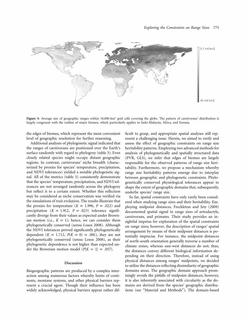
Exploring the Constraints on Range Sizes 775

Figure 3: Average size of geographic ranges within 10,000-km2 grid cells covering the globe. The pattern of carnivorans’ distribution islargely congruent with the outline of major biomes, which particularly applies in Indo-Malaysia, Africa, and Eurasia.

the edges of biomes, which represent the most convenientlevel of geographic resolution for further reasoning.

Additional analyses of phylogenetic signal indicated thatthe ranges of carnivorans are positioned over the Earth’ssurface randomly with regard to phylogeny (table 3). Evenclosely related species might occupy distant geographicregions. In contrast, carnivorans’ niche breadth (charac-terized by proxies for species’ temperature, precipitation,and NDVI tolerances) yielded a notable phylogenetic sig-nal. All of the metrics (table 3) consistently demonstratethat the species’ temperature, precipitation, and NDVI tol-erances are not arranged randomly across the phylogenybut reflect it to a certain extent. Whether this reflectionmay be considered as niche conservatism was verified viathe simulations of trait evolution. The results illustrate thatthe proxies for temperature ( , ) andK p 1.996 P p .022precipitation ( , ) tolerance signifi-K p 1.912 P p .023cantly diverge from their values as expected under Brown-ian motion (i.e., ); hence, we can consider themK p 1phylogenetically conserved (sensu Losos 2008). Althoughthe NDVI tolerances proved significantly phylogeneticallydependent ( , ), they are notK p 1.712 P(K p 0) p .001phylogenetically conserved (sensu Losos 2008), as theirphylogenetic dependence is not higher than expected un-der the Brownian motion model .(P[K p 1] p .057)

Discussion

Biogeographic patterns are produced by a complex inter-action among numerous factors whereby limits of conti-nents, montane systems, and other physical barriers rep-resent a crucial agent. Though their influence has beenwidely acknowledged, physical barriers appear rather dif-

ficult to grasp, and appropriate spatial analyses still rep-resent a challenging issue. Herein, we aimed to verify andassess the effect of geographic constraints on range sizeheritability patterns. Employing two advanced methods foranalysis of phylogenetically and spatially structured data(PVR, GLS), we infer that edges of biomes are largelyresponsible for the observed patterns of range size heri-tability. Furthermore, we propose a mechanism wherebyrange size heritability patterns emerge due to interplaybetween geographic and phylogenetic constraints. Phylo-genetically conserved physiological tolerances appear toshape the extent of geographic domains that, subsequently,underlie species’ range size.

So far, spatial constraints have only rarely been consid-ered when studying range sizes and their heritability. Em-ploying midpoint distances, Freckleton and Jetz (2009)documented spatial signal in range sizes of artiodactyls,carnivorans, and primates. Their study provides an in-sightful impetus for exploration of the spatial constraintson range sizes; however, the description of ranges’ spatialarrangement by means of their midpoint distances is po-tentially imprecise. For instance, the midpoint distancesof north-south orientation generally traverse a number ofclimate zones, whereas east-west distances do not; thus,the distances convey different biological information de-pending on their direction. Therefore, instead of usingphysical distances among ranges’ midpoints, we decidedto utilize the distances reflecting dissimilarity of geographicdomains areas. The geographic domain approach prom-isingly avoids the pitfalls of midpoint distances; however,it is also inherently associated with circularity as the do-mains are derived from the species’ geographic distribu-tions (see “Material and Methods”). The domain-based

776 The American Naturalist

Table 3: Phylogenetic signal in niche breadth and range geographic position as evaluated by Blomberg’s K, Pagel’s l, andMoran’s I

Blomberg’s KP

(K p 0)P

(K p 1) Moran’s IP

(I p 0) Pagel’s l

P(l p 1)

P(l p 0)

Niche breadth:Log(temperature) SD 1.996 .001 .022 .856 .007 .997 .994 .001Log(precipitation) SD 1.912 .001 .023 .823 .011 .997 .994 .001Log(NDVI) SD 1.712 .001 .057 .695 .036 .996 .990 .001

Geographic position:Midpoint distances .005 .005 .001 .015 .059 .073 .001 .001Geographic coordinates .001 .998 .001 .003 .989 .689 .023 .047

Note: P values are indicated along with the null hypothesis tested. In sum, the geographic position of ranges proved virtually no phylogenetic dependence

( , , ). The phylogenetic dependence in the case of normalized difference vegetation index (NDVI) tolerance was consistent with the expectationsK ≈ 0 I ≈ 0 l ! 1

under the Brownian motion model of trait evolution ( , ). Phylogenetic conservatism was detected in the case of temperature and precipitationK ≈ 1 l ≈ 1

tolerances ( , ), as their values were significantly more similar than expected under Brownian motion.K 1 1 P[K p 1] ! .025

approach revealed a noticeable spatial signal in carnivoranrange sizes.

Unlike Mouillot and Gaston (2009), we used Moran’sI rather than sister-species pair comparison to examinerange size heritability. Hence, we could utilize all of theinformation conveyed by a phylogenetic tree (i.e., not onlyby sister species) and also explore heritability patternsabove the species level (fig. 2). This is particularly im-portant as heritability patterns have been documented tovary among taxonomic levels (Jones et al. 2005; appendixsection “Analyses of Phylogenetic Signal”). Despite em-ploying a different methodical approach than Mouillot andGaston (2009), we arrive at the same conclusion that rangesizes are considerably spatially dependent.

Our finding that biome domains are largely responsiblefor the carnivoran range sizes contrasts with conclusionsof Bohning-Gaese et al. (2006) based on 26 bird species.It is possible that range sizes of birds and carnivorans areconstrained differently, but also that the group of 26 Sylviawarblers studied by Bohning-Gaese et al. (2006) was ratheratypical due to the specifics of their life history. Since ourconclusions are founded on a data set of 231 carnivorans,they are liable to be plausible and of more generalrelevance.

The outcomes of our analyses provide different conclu-sions for different levels of domains’ delimitation (i.e.,continents, biomes, and climate envelopes). When the geo-graphic constraints of continental domains or range mid-point distances are considered, phylogeny appears as themajor agent responsible for the range size variation. Incontrast, detailed description of geographic constraints interms of biomes and climate envelopes proves phylogenyto be of only marginal importance, so that the geographicconstraints underlie the range sizes over and above theeffects of phylogeny. This situation is in fact fairly char-acteristic. The finding that the obtained results depend onhow the model is constructed (i.e., the effect of geographic

domains depending on the geographic resolution in ourcase) has been recognized since the early 1970’s in thecontext of community assembly rules and their null mod-els (Wilson 1995; Stone et al. 1996; Gotelli 2001). It hasturned out that there is no “correct” null model, onlymodels differing in the amount of information used fortheir construction. If considerable prior information aboutthe system is used for the construction of the model (i.e.,delimitation of biomes or climate envelopes in our case),the model usually proves plausible, but it is a simple con-sequence of the fact that the pattern is already somehowcontained in the model, a situation sometimes called “thenarcissus effect” (Gotelli 2001). From this point of view,it makes no sense to ask whether range size heritabilitycan be attributed to the geographic constraints but ratherhow precise definition of the constraints is necessary fora concise description of the range size patterns (see fig.3). In this light, our conclusion that the more compre-hensive the definition of geographic domain, the greaterits effect on range size in comparison to phylogeny, is notparticularly surprising.

In fact, our findings do not reject the effect of phylogenyon range size but rather imply the mechanisms underlyingthe range size heritability patterns. We have shown thatheritability is largely driven by the extent of biomes; how-ever, this extent appears to be determined by phylogenybecause related species share temperature and precipita-tion tolerances (table 3) as well as habitat and environ-mental preferences (Peterson et al. 1999; Diniz-Filho et al.2010). Thus, bound by common evolutionary history, re-lated species are limited in their distribution by similargeographic constraints. As these constraints represent amore proximate factor shaping species’ ranges, they ac-count for more of the range size variation than phylogenydoes. Thus, the range size heritability patterns presumablyemerge as a consequence of this interplay between evo-lutionary and geographic constraints.

Exploring the Constraints on Range Sizes 777

Since the biome domains account for approximately50% of the range size variation ( , ; tables2R ≈ 0.50 F ≈ 0.851, 2), they appear to be the major single factor responsiblefor range size heritability patterns, at least in carnivorans.The other proposed mechanisms of range size heritability(dispersal ability, physiological tolerances, functionalgroup membership; Mouillot and Gaston 2009) are eithersubcategories of geographic constraints or phenomena ofrather marginal importance. Since geographic position ofcarnivoran ranges exhibits no phylogenetic pattern (table3; Cox and Moore 2005), range size heritability is notunderlain by shared physical barriers (i.e., related speciesbeing limited by identical rivers, mountain ranges, orcoastline), as even geographically distant species occupyranges of similar extent (table 3). With respect to ourresults, phylogenetically conserved niche breadth, whichdetermines the size of geographic domains, appears to bethe crucial driver of range size heritability. Nonetheless,we note as a caveat that we comply with the general prac-tice and interpret high phylogenetic signal in niche breadth(table 3) as evidence for niche conservatism (Blomberg etal. 2003; Swenson and Enquist 2007), although some stud-ies have challenged such interpretation (e.g., Revell et al.2008).

Our findings imply that despite being emergent only atthe species level, geographic range size is associated withindividual-level traits (i.e., physiological tolerance andniche breadth). Therefore, we conclude that the range sizeheritability phenomenon does not necessarily enforce thespecies selection concept as range size heritability can bedirectly linked to the natural selection that operates on thelevel of individuals.

Acknowledgments

We are indebted to R. P. Freckleton for kindly supplyingthe R code that implements the phylogenetic/spatial GLSanalyses. We are also grateful to E. Pechlakova, A. Sizling,P. Smilauer, F. Zemek, and anonymous reviewers for com-ments and advice that have greatly improved our manu-script. A.M. was supported by the J. W. Fulbright Com-mission. D.S. was supported by the Grant Agency of theCzech Republic (P505/11/2387) and by the Czech Ministryof Education (MSM0021620845).

Literature Cited

Arnason, U., A. Gullberg, A. Janke, and M. Kullberg. 2007. Mito-genomic analyses of caniform relationships. Molecular Phyloge-netics and Evolution 45:863–874.

Bardeleben, C., R. L. Moore, and R. K. Wayne. 2005. A molecular

phylogeny of the Canidae based on six nuclear loci. MolecularPhylogenetics and Evolution 37:815–831.

Baum, B. R. 1992. Combining trees as a way of combining data setsfor phylogenetic inference and the desirability of combining genetrees. Taxon 41:3–10.

Bininda-Emonds, O. R. P., J. L. Gittleman, and A. Purvis. 1999.Building large trees by combining phylogenetic information: acomplete phylogeny of the extant Carnivora (Mammalia). Bio-logical Reviews 74:143–175.

Bivand, R., L. Anselin, R. Assuncao, and O. Berke. 2008. Spatialdependence: weighting schemes, statistics and models. R pack-age, version 0.4-21. http://cran.r-project.org/web/packages/spdep/index.html.

Blackburn, T. M. 2004. Method in macroecology. Basic and AppliedEcology 5:401–412.

Blomberg, S. P., T. Garland Jr., and A. R. Ives. 2003. Testing forphylogenetic signal in comparative data: behavioral traits are morelabile. Evolution 57:717–745.

Bohning-Gaese, K., T. Caprano, K. van Ewijk, and M. Veith. 2006.Range size: disentangling current traits and phylogenetic and bio-geographic factors. American Naturalist 167:555–567.

Brown, J. H., G. C. Stevens, and D. M. Kaufman. 1996. The geo-graphic range: size, shape, boundaries, and internal structure. An-nual Review of Ecology and Systematics 27:597–623.

Carrascal, L. M., J. Seoane, D. Palomino, and V. Polo. 2008. Expla-nations for bird species range size: ecological correlates and phy-logenetic effects in the Canary Islands. Journal of Biogeography35:2061–2073.

Cox, C. B., and P. B. Moore. 2005. Biogeography: an ecological andevolutionary approach. Blackwell, Malden.

Cubo, J., F. Ponton, M. Laurin, E. de Margerie, and J. Castanet. 2005.Phylogenetic signal in bone microstructure of sauropsids. System-atic Biology 54:562–574.

Currie, D. J. 1991. Energy and large-scale patterns of animal-speciesand plant-species richness. American Naturalist 137:27–49.

Diniz-Filho, J. A., and L. M. Bini. 2005. Modelling geographicalpatterns in species richness using eigenvector-based spatial filters.Global Ecology and Biogeography 14:177–185.

Diniz-Filho, J. A., and N. M. Torres. 2002. Phylogenetic comparativemethods and the geographic range size–body size relationship inNew World terrestrial carnivora. Evolutionary Ecology 16:351–367.

Diniz-Filho, J. A. F., L. C. Terribile, M. J. R. da Cruz, and L. C. G.Vieira. 2010. Hidden patterns of phylogenetic non-stationarityoverwhelm comparative analyses of niche conservatism and di-vergence. Global Ecology and Biogeography 19: 916–926.

Elith, J., C. H. Graham, R. P. Anderson, M. Dudik, S. Ferrier, A.Guisan, R. J. Hijmans, et al. 2006. Novel methods improve pre-diction of species’ distributions from occurrence data. Ecography29:129–151.

Fortes, R. R., and R. S. Absalao. 2004. The applicability of Rapoport’srule to the marine molluscs of the Americas. Journal of Bioge-ography 31:1909–1916.

Freckleton, R. P., and W. Jetz. 2009. Space versus phylogeny: dis-entangling phylogenetic and spatial signals in comparative data.Proceedings of the Royal Society B: Biological Sciences 276:21–30.

Freckleton, R. P., P. H. Harvey, and M. Pagel. 2002. Phylogeneticanalysis and comparative data: a test and review of evidence. Amer-ican Naturalist 160:712–726.

Freckleton, R. P., N. Cooper, and W. Jetz. 2011. Comparative methods

778 The American Naturalist

as a statistical fix: the dangers of ignoring evolution. AmericanNaturalist (forthcoming).

Fulton, T. L., and C. Strobeck. 2006. Molecular phylogeny of theArctoidea (Carnivora): effect of missing data on supertree andsupermatrix analyses of multiple gene data sets. Molecular Phy-logenetics and Evolution 41:165–181.

Gaston, K. J. 2003. The structure and dynamics of geographic ranges.Oxford University Press, Oxford.

Gaston, K. J., T. M. Blackburn, and J. I. Spicer. 1998. Rapoport’srule: time for an epitaph? Trends in Ecology & Evolution 13:70–74.

Gaubert, P., and C. M. Begg. 2007. Re-assessed molecular phylogenyand evolutionary scenario within genets (Carnivora, Viverridae,Genettinae). Molecular Phylogenetics and Evolution 44:920–927.

Gaubert, P., and P. Cordeiro-Estrela. 2006. Phylogenetic systematicsand tempo of evolution of the Viverrinae (Mammalia, Carnivora,Viverridae) within feliformians: implications for faunal exchangesbetween Asia and Africa. Molecular Phylogenetics and Evolution41:266–278.

Gittleman, J. L. 1996. Carnivore behavior, ecology, and evolution.Cornell University Press, Ithaca, NY.

Gittleman, J. L., and M. Kot. 1990. Adaptation: statistics and a nullmodel for estimating phylogenetic effects. Systematic Zoology 39:227–241.

Goloboff, P. A. 1999. NONA. Version 2.0 (software and manual).Fundacion e Instituto Miguel Lillo, Tucuman, Argentina.

Gotelli, N. J. 2001. Research frontiers in null model analysis. GlobalEcology and Biogeography 10:337–343.

Gould, S. J., and E. A. Lloyd. 1999. Individuality and adaptationacross levels of selection: how shall we name and generalize theunit of Darwinism? Proceedings of the National Academy of Sci-ences of the USA 96:11904–11909.

Grantham, T. A. 1995. Hierarchical approaches to macroevolution:recent work on species selection and the effect hypothesis. AnnualReview of Ecology and Systematics 26:301–321.

Guisan, A., and W. Thuiller. 2005. Predicting species distribution:offering more than simple habitat models. Ecology Letters 8:993–1009.

Guisan, A., and N. E. Zimmermann. 2000. Predictive habitat distri-bution models in ecology. Ecological Modelling 135:147–186.

Harmon, L. J., J. T. Weir, C. D. Brock, R. E. Glor, and W. Challenger.2008. GEIGER: investigating evolutionary radiations. Bioinfor-matics 24:129–131.

Hijmans, R. J., S. E. Cameron, J. L. Parra, P. G. Jones, and A. Jarvis.2005. Very high resolution interpolated climate surfaces for globalland areas. International Journal of Climatology 25:1965–1978.

Hunt, G., K. Roy, and D. Jablonski. 2005. Species-level heritabilityreaffirmed: a comment on “On the heritability of geographic rangesizes.” American Naturalist 166:129–135.

Hurlbert, A. H., and W. Jetz. 2007. Species richness, hotspots, andthe scale dependence of range maps in ecology and conservation.Proceedings of the National Academy of Sciences of the USA 104:13384–13389.

IUCN (International Union for Conservation of Nature). 2010. TheIUCN Red List of Threatened Species. http://www.iucnredlist.org.

Jablonski, D. 1987. Heritability at the species level: analysis of geo-graphic ranges of cretaceous mollusks. Science 238:360–363.

———. 2008. Species selection: theory and data. Annual Review ofEcology, Evolution, and Systematics 39:501–524.

Johnson, W. E., E. Eizirik, J. Pecon-Slattery, W. J. Murphy, A. An-

tunes, E. Teeling, and S. J. O’Brien. 2006. The Late Miocene ra-diation of modern Felidae: a genetic assessment. Science 311:73–77.

Jones, K. E., W. Sechrest, and J. L. Gittleman. 2005. Age and arearevisited: identifying global patterns and implications for conser-vation. Pages 141–165 in A. Purvis, J. L. Gittleman, and T. Brooks,eds. Phylogeny and conservation. Cambridge University Press,Cambridge.

Kadmon, R., O. Farber, and A. Danin. 2003. A systematic analysisof factors affecting the performance of climatic envelope models.Ecological Applications 13:853–867.

Kembel, S. W., P. D. Cowan, M. R. Helmus, W. K. Cornwell, H.Morlon, D. D. Ackerly, S. P. Blomberg, and C. O. Webb. 2010.Picante: R tools for integrating phylogenies and ecology. Bioin-formatics 26:1463–1464.

Koepfli, K. P., S. M. Jenks, E. Eizirik, T. Zahirpour, B. Van Valken-burgh, and R. K. Wayne. 2006. Molecular systematics of the Hyaen-idae: relationships of a relictual lineage resolved by a molecularsupermatrix. Molecular Phylogenetics and Evolution 38:603–620.

Koepfli, K. P., M. E. Gompper, E. Eizirik, C. C. Ho, L. Linden, J. E.Maldonado, and R. K. Wayne. 2007. Phylogeny of the Procyonidae(Mammalia: Carnivora): molecules, morphology and the GreatAmerican Interchange. Molecular Phylogenetics and Evolution 43:1076–1095.

Koepfli, K. P., K. A. Deere, G. J. Slater, C. Begg, K. Begg, L. Grassman,M. Lucherini, G. Veron, and R. K. Wayne. 2008. Multigene phy-logeny of the Mustelidae: resolving relationships, tempo and bio-geographic history of a mammalian adaptive radiation. BMC Bi-ology 6, http://www.biomedcentral.com/1741-7007/6/10.

Krause, J., T. Unger, A. Nocon, A. S. Malaspinas, S. O. Kolokotronis,M. Stiller, L. Soibelzon, et al. 2008. Mitochondrial genomes revealan explosive radiation of extinct and extant bears near the Mio-cene-Pliocene boundary. BMC Evolutionary Biology 8, http://www.biomedcentral.com/1471-2148/8/220.

Legendre, P., M. R. T. Dale, M. J. Fortin, J. Gurevitch, M. Hohn,and D. Myers. 2002. The consequences of spatial structure for thedesign and analysis of ecological field surveys. Ecography 25:601–615.

Lindblad-Toh, K., C. M. Wade, T. S. Mikkelsen, E. K. Karlsson, D.B. Jaffe, M. Kamal, M. Clamp, et al. 2005. Genome sequence,comparative analysis and haplotype structure of the domestic dog.Nature 438:803–819.

Liu, F. G. R., M. M. Miyamoto, N. P. Freire, P. Q. Ong, M. R. Tennant,T. S. Young, and K. F. Gugel. 2001. Molecular and morphologicalsupertrees for eutherien (placental) mammals. Science 291:1786–1789.

Losos, J. B. 2008. Phylogenetic niche conservatism, phylogenetic sig-nal and the relationship between phylogenetic relatedness and eco-logical similarity among species. Ecology Letters 11:995–1003.

Machac, A., M. Janda, R. R. Dunn, and N. J. Sanders. 2010. Eleva-tional gradients in phylogenetic structure of ant communities re-veal the interplay of biotic and abiotic constraints on diversity.Ecography (forthcoming), doi:10.1111/j.1600-0587.2010.06629.x.

Mouillot, D., and K. Gaston. 2009. Spatial overlap enhances geo-graphic range size conservatism. Ecography 32:671–675.

Olson, D. M., E. Dinerstein, E. D. Wikramanayake, N. D. Burgess,G. V. N. Powell, E. C. Underwood, J. A. D’Amico, et al. 2001.Terrestrial ecoregions of the worlds: a new map of life on Earth.BioScience 51:933–938.

Pagel, M. D., R. M. May, and A. R. Collie. 1991. Ecological aspects

Exploring the Constraints on Range Sizes 779

of the geographical distribution and diversity of mammalian spe-cies. American Naturalist 137:791–815.

Paradis, E., J. Claude, and K. Strimmer. 2004. APE: analyses of phy-logenetics and evolution in R language. Bioinformatics 20:289–290.

Patou, M. L., R. Debruyne, A. P. Jennings, A. Zubaid, J. J. Rovie-Ryan, and G. Veron. 2008. Phylogenetic relationships of the Asianpalm civets (Hemigalinae & Paradoxurinae, Viverridae, Carni-vora). Molecular Phylogenetics and Evolution 47:883–892.

Patou, M. L., P. A. McLenachan, C. G. Morley, A. Couloux, A. P.Jennings, and G. Veron. 2009. Molecular phylogeny of the Her-pestidae (Mammalia, Carnivora) with a special emphasis on theAsian Herpestes. Molecular Phylogenetics and Evolution 53:69–80.

Pechlakova, E. 2006. Macroecology of the Carnivora: patterns in thegeographic ranges with respect to phylogeny. MSc thesis. Univer-sity of South Bohemia, Ceske Budejovice.

Peterson, A. T., J. Soberon, and V. Sanchez-Cordero. 1999. Conser-vatism of ecological niches in evolutionary time. Science 285:1265–1267.

Rabosky, D. L., and A. R. McCune. 2010. Reinventing species selec-tion with molecular phylogenies. Trends in Ecology & Evolution25:68–74.

Ragan, M. A. 1992. Phylogenetic inference based on matrix repre-sentation of trees. Molecular Phylogenetics and Evolution 1:53–58.

Rahbek, C., and G. R. Graves. 2001. Multiscale assessment of patternsof avian species richness. Proceedings of the National Academy ofSciences of the USA 98:4534–4539.

Rangel, T., J. A. F. Diniz-Filho, and L. M. Bini. 2006. Towards anintegrated computational tool for spatial analysis in macroecologyand biogeography. Global Ecology and Biogeography 15:321–327.

R Development Core Team. 2009. R: a language and environmentfor statistical computing. R Foundation for Statistical Computing,Vienna.

Revell, L. J., L. J. Harmon, and D. C. Collar. 2008. Phylogeneticsignal, evolutionary process, and rate. Systematic Biology 57:591–601.

Ricklefs, R. E., and R. E. Latham. 1992. Intercontinental correlationof geographical ranges suggests stasis in ecological traits of relictgenera of temperate perennial herbs. American Naturalist 139:1305–1321.

Sato, J. J., M. Wolsan, S. Minami, T. Hosoda, M. H. Sinaga, K.

Hiyama, Y. Yamaguchi, and H. Suzuki. 2009. Deciphering anddating the red panda’s ancestry and early adaptive radiation ofMusteloidea. Molecular Phylogenetics and Evolution 53:907–922.

Smith, F. D. M., R. M. May, and P. H. Harvey. 1994. Geographicalranges of Australian mammals. Journal of Animal Ecology 63:441–450.

Soberon, J., and M. Nakamura. 2009. Niches and distributional areas:concepts, methods, and assumptions. Proceedings of the NationalAcademy of Sciences of the USA 106:19644–19650.

Stone, L., T. Dayan, and D. Simberloff. 1996. Community-wide as-sembly patterns unmasked: the importance of species’ differinggeographical ranges. American Naturalist 148:997–1015.

Swenson, N. G., and B. J. Enquist. 2007. Ecological and evolutionarydeterminants of a key plant functional trait: wood density and itscommunity-wide variation across latitude and elevation. AmericanJournal of Botany 94:451–459.

Taylor, C. M., and N. J. Gotelli. 1994. The macroecology of Cyprinella:correlates of phylogeny, body size, and geographical range. Amer-ican Naturalist 144:549–569.

ter Braak, C. J. F., and P. Smilauer 2002. CANOCO 4.5 referencemanual and CanoDraw for Windows. User’s guide to CANOCOfor Windows: software for canonical community ordination. Mi-crocomputer Power, Ithaca, NY.

Tucker, C. J., J. E. Pinzon, M. E. Brown, D. A. Slayback, E. W. Pak,R. Mahoney, E. F. Vermote, and N. El Saleous. 2005. An extendedAVHRR 8-km NDVI dataset compatible with MODIS and SPOTvegetation NDVI data. International Journal of Remote Sensing26:4485–4498.

Waldron, A. 2007. Null models of geographic range size evolutionreaffirm its heritability. American Naturalist 170:221–231.

Webb, C. O., D. D. Ackerly, and S. W. Kembel. 2008. Phylocom:software for the analysis of phylogenetic community structure andtrait evolution. Bioinformatics 24:2098–2100.

Webb, T. J., and K. J. Gaston. 2003. On the heritability of geographicrange sizes. American Naturalist 161:553–566.

———. 2005. Heritability of geographic range sizes revisited: a replyto Hunt et al. American Naturalist 1646:136–143.

Wilson, J. B. 1995. Null models for assembly rules: the Jack Hornereffect is more insidious than the narcissus effect. Oikos 72:139–144.

Associate Editor: Axel G. RossbergEditor: Judith L. Bronstein