Randomly coloring random graphs

Randomly Coloring Random Graphs*

Martin Dyer,1 Alan Frieze2

1School of Computing, University of Leeds, Leeds LS2 9JT, UK;e-mail: [email protected]

2Department of Mathematical Sciences, Carnegie Mellon University,Pittsburgh, Pennsylvania; e-mail: [email protected]

Received 12 May 2008; accepted 18 December 2008Published online 24 August 2009 in Wiley InterScience (www.interscience.wiley.com).DOI 10.1002/rsa.20286

ABSTRACT: We consider the problem of generating a coloring of the random graph Gn,p uniformlyat random using a natural Markov chain algorithm: the Glauber dynamics. We assume that there areβ� colors available, where � is the maximum degree of the graph, and we wish to determine theleast β = β(p) such that the distribution is close to uniform in O(n log n) steps of the chain. Thisproblem has been previously studied for Gn,p in cases where np is relatively small. Here we considerthe “dense” cases, where np ∈ [ω ln n, n] and ω = ω(n) → ∞. Our methods are closely tailoredto the random graph setting, but we obtain considerably better bounds on β(p) than can be achievedusing more general techniques. © 2009 Wiley Periodicals, Inc. Random Struct. Alg., 36, 251–272, 2010

Keywords: random colorings; random graphs; Glauber dynamics

1. INTRODUCTION

This article is concerned with the problem of randomly coloring a graph with a givennumber of colors. The coloring should be proper in the sense that adjacent vertices getdifferent colors and the distribution of the coloring should be close to uniform over the setof possible colorings. This problem has been the subject of intense study by researchersinto Markov Chain Monte Carlo Algorithms (MCMC). In spite of this, the problem is notwell solved.

Jerrum [10] showed that if � denotes the maximum degree of G and the number ofcolors q ≥ 2�, then a simple algorithm can be used to generate a near random coloring inpolynomial time. Vigoda [14] used a more complicated Markov Chain and improved this toq ≥ 11�/6. In spite of almost 10 years of effort, this is still the best bound known for thegeneral case. Dyer and Frieze [4] were able to improve this bound by restricting attention to

Correspondence to: A. Frieze*Supported by EPSRC(EP/E062172/1); NSF (CCF-0502793).© 2009 Wiley Periodicals, Inc.

251

252 DYER AND FRIEZE

graphs of large enough maximum degree and large enough girth. There have been severalimprovements to this latter result and Frieze and Vigoda [5] surveys most of the knownresults.

The article of Dyer, Flaxman, Frieze and Vigoda [3] considered this question in relationto random graphs, trying to bound the number of colors needed by something other than themaximum degree. They considered the random graph Gn,p with edge probability p = d/n,d constant and gave an upper bound on the number of colors needed that was o(�) whp.Mossel and Sly [13] have improved this result and shown that whp the number of colorsneeded satisfies q ≤ qd where qd depends only on d. The random graph Gn,p is the subjectof this article, but we consider graphs which are denser than those discussed in [3] and [13].We will discuss the range np ∈ [ω ln n, n] where ω = ω(n) → ∞.

2. GLAUBER DYNAMICS

We consider colorings X : V → C of a graph G, with color set C = [q]. If V ′ ⊆ V , we usethe notation X(V ′) = {X(v) : v ∈ V ′}. A coloring is proper if X(v) �= X(w) (∀{v, w} ∈ E),but here colorings should not be assumed proper unless this is stated. The set of all propercolorings of G will be denoted by �G, with NG = |�G|.

We consider the Metropolis Glauber dynamics on the set Cn of all colorings of V . Forany coloring X of a graph G, the Metropolis update is defined as follows.

1: function Update(X)2: X′ ← X3: choose u ∈ V and c ∈ C uar4: if ∀w ∈ Nu: X′(w) �= c then5: X′(u) ← c6: return X′

We will refer to steps 4-5 as an update of vertex u. An update will be called successfulif Step 4 is executed, otherwise unsuccessful.

We analyze the following Markov chain Xt based on these dynamics, with initialcoloring X:

1: function Glauber(X, t)2: X0 ← X3: for t ← 1 to t do4: Xt ← Update(Xt−1)

5: return Xt

We say the tth update occurs at time t, and the vertex and colour used are denotedby ut , ct .

For any initial coloring X, the equilibrium distribution πG of Glauber(X, ∞) is uniformon the set �G. Thus πG(X) = 1/NG (∀X ∈ �G), and πG is invariant under an update of anyvertex.

Let τ(ε) = mint{dTV(Xt , πG) ≤ ε}. Here dTV is the total variation distance betweendistributions (see [11, p. 26]), and τ(ε) is called the mixing time. Our chain will be saidto be rapidly mixing if for any initial coloring X and any fixed ε, τ(ε) is bounded by apolynomial in n. Our aim is to find sufficient conditions for the chain to be rapidly mixing.

Random Structures and Algorithms DOI 10.1002/rsa

RANDOMLY COLORING RANDOM GRAPHS 253

2.1. Random Graphs and Colorings

Let V (2) denote the set of all pairs {v, w} (v, w ∈ V , v �= w). Then Gn,p will denote theErdos-Rényi probability space on Gn. A random graph G = (V , E) from this distribution isdefined by

Pr({v, w} ∈ E) = p, independently for all pairs {v, w} ∈ V (2).

See, for example, [9] for further information.We consider p(n) ≥ ω(n) ln n/n, where ω(n) → ∞ slowly, so that (say) ω =

o(log log n). We also assume 1 − p(n) = �(1) as n → ∞.We say that an event E occurs with high probability (whp) if Pr(E) ≥ 1 − n−k for all

k ≥ 0. If events Ej (j ∈ J) occur whp, it follows that the event⋃

j∈J Ej also occurs whp,whenever |J| is bounded by any polynomial in n. We will call this the union bound.

We now define some constants that are used in our main theorem. First let β0 =1.48909 . . . be the solution to

βe−1/β + (1 − e−1/β)2 = 1.

Now define β1 ≈ 1.63457 to be the solution to

κ1(β) + βe−1/β = 1

where

κ1(β) = 2

β

∫ 1

0(1 − e−x/β) exp

(− x

β−

∫ x

0

dy

e(1−y)/β − y

)dx. (1)

In the next definition η represents an arbitrarily small positive constant. Let

β(p) = (1 + η) ×

β0 ω ln n/n ≤ p = o(1/ ln n)

β1 �(1/ ln n) ≤ p = o(1)

β2(p) p = �(1)

The definition of β2(p) is complex and Fig. 3 below provides a numerical plot.The number of colors available will be parameterized as β� ≈ βnp1 , since whp every

vertex of Gn,p will have vertex degree ≈ np.

Theorem 1. If G = Gn,p then Glauber Dynamics mixes in O(n ln n) time whp providedβ ≥ β(p).

Some comments are in order. The value β0 appears in Molloy [12] where q > β0� isshown to be sufficient for rapid mixing when � = �(ln n) and the girth is �(log �). Theimportant point to note is that for our range of values for p and for almost all choices ofGn,p, nothing better than Vigoda’s bound of 11np/6 can be inferred by previous results. Itis perhaps of interest to point out here that whp χ(Gn,p) ≈ np

2 log np .

1An ≈ Bn iff An = (1 + o(1))Bn as n → ∞.


254 DYER AND FRIEZE

3. PROOF OF THEOREM 1

3.1. Proof Strategy

We make use of a particular choice of random initial distribution.

1: function Random2: for v ∈ V do3: choose X(v) ∈ C uar4: return X

This initial coloring is unlikely to be a proper coloring of G, but it is independent ofE. We will analyze Glauber(Random, t0), t0 = �λn ln n (the value of λ is given inSection 3.3). We will show in Lemmas 1, 2 below that this chain has nice properties. Wecouple the chains Glauber(Y, t0), where Y ∼ πG

2, and Glauber(Random, t0). Using theaforementioned properties we show that these two chains will tend to coincide rapidly. Wededuce that the equilibrium distribution also has the same nice properties. We can then usethese properties to show convergence of Glauber(X0, t0) for an arbitrary initial coloringX0. This is achieved by coupling the chains Glauber(Y, t0) and Glauber(X0, t0).

3.2. Coupling Argument

Let Gn = {G = (V , E) : V = [n]} be the set of n-vertex graphs. If G ∈ Gn, the set ofneighbors of a vertex v ∈ V will be denoted by Nv = {w ∈ V : {v, w} ∈ E}, and its degreedv = |Nv|. The maximum degree of G is �(G) = maxv∈V dv.

If X is a coloring of G and v ∈ V , let

Av(X) = {c ∈ C : X(w) �= c, ∀w ∈ Nv}be the set of colors which are available for a successful update of v. Also, let Av(X) =|Av(X)|. Clearly we always have Av(X) ≥ q − � = (β − 1)�.

We prove convergence of Glauber using a coupling due to Jerrum [10] and an idea ofHayes and Vigoda [7]. In [7] an arbitrary chain is coupled with one started in an equilibriumdistribution whose properties are known. We use the following coupling, which is essentiallythat used by Jerrum [10]. Let uX , cX and uY , cY be the choices in Step 3 of Update(Xt) andUpdate(Yt), respectively.

1: procedure Couple(X , Y)

2: Choose u ∈ V uar3: uX ← u, uY ← u4: AX ← Au(X), AY ← Au(Y)

5: AX ← |AX |, AY ← |AY |6: Construct a bijection f : C → C such that7: f (c) ← c (∀c ∈ AX ∩ AY )8: if AX ≤ AY then f (AX) ⊆ AY else f (AY ) ⊆ AX

9: Choose c ∈ C uar10: cX ← c, cY ← f (c)

2We use ∼ to denote has the same distribution as.



Note that Couple ensures that cY will be sampled uar from C, as required. For brevity,we will make use of the notation defined in Couple below.

Let X ′, Y ′ be the colorings after updating X and Y with u, cX = c, cY = f (c) chosen byCouple. Let W = {w ∈ V : X(w) �= Y(w)} and W = |W| = d(X, Y), where d(·, ·) is theHamming distance. For any v ∈ V , let Wv = W ∩ Nv and Wv = |Wv|. Note that

∑v∈V

Wv ≤∑w∈W

dw ≤ �W .

Note that c ∈ AX \ AY implies there is a w ∈ Nu such that X(w) �= c and Y(w) = c. Hence|AX \ AY | ≤ Wu, and similarly |AY \ AX | ≤ Wu. Let

Au = max{AX , AY }

so that we have

Au − |AX ∩ AY | = max{|AX \ AY |, |AY \ AX |} ≤ Wu. (2)

Also, from Step 8 of Couple, there are q − Au pairs c, f (c) such that c /∈ AX , f (c) /∈ AY .Hence there are at most Au − |AX ∩ AY | ≤ Wu pairs which result in X ′(u) �= Y ′(u). LettingW ′ = d(X ′, Y ′), and assuming that we have a bound

Au ≥ α� (3)

for some α > 1 that holds whp for all t ≤ n2 say, then we have

E[W ′ − W ] ≤ −∑u∈W

Au − Wu

nq+

∑u/∈W

Wu

nq≤ −α�W

nq+

∑u∈V

Wu

nq

≤ −α�W

nq+ �W

nq= − (α − 1)W

nβ, (4)

since q = β�.Therefore,

E[W ′] ≤(

1 − α − 1

nβ

)W . (5)

Using the Coupling Lemma (see [11, Lemma 4.7]),

dTV(Xt , Yt) ≤ Pr(Xt �= Yt) ≤ E[d(Xt , Yt)] ≤ n

(1 − α − 1

nβ

)t

≤ ne−(α−1)t/nβ ≤ ε,

for t ≥ βn ln(n/ε)/(α − 1).Thus, one part of the analysis involves finding a lower bound as in (3).A further improvement is possible using a modification of a method of Molloy [12].

Now, for any v ∈ V , let us define

W∗v = {w ∈ Nv : X(w) /∈ Y(Nv) ∨ Y(w) /∈ X(Nv)}, and W ∗

v = |W∗v |.


256 DYER AND FRIEZE

Note that W∗v ⊆ Wv, so W ∗

v ≤ Wv, since X(w) = Y(w) clearly implies X(w) ∈ Y(Nv) andY(w) ∈ X(Nv). Also, we will define

N ∗v = {w ∈ Nv : X(v) /∈ Y(Nw) ∨ Y(v) /∈ X(Nw)} and d∗

v = |N ∗v |. (6)

We obviously have N ∗v ⊆ Nv, and hence d∗

v ≤ dv. Note also that w ∈ N ∗v iff v ∈ W∗

w.Furthermore, N ∗

v = ∅ if X(v) = Y(v), since this implies X(v) ∈ Y(Nw) and Y(v) ∈ X(Nw)

for all w ∈ Nv. Thus d∗v = 0 for all v /∈ W . Hence,∑

v∈V

W ∗v =

∑w∈W

d∗w.

Note that c ∈ AX \AY implies there is a w ∈ Nu such that Y(w) = c and c /∈ X(Nu). Hence|AX \ AY | ≤ W ∗

u , and similarly |AY \ AX | ≤ W ∗u . Hence

Au − |AX ∩ AY | = max{|AX \ AY |, |AY \ AX |} ≤ W ∗u .

which is a strengthening of (2).So,

W ′ − W ≤ −∑u∈W

Au − W ∗u

nq+

∑u/∈W

W ∗u

nq≤ −αW

nq+

∑u∈V

W ∗u

nq= −αW

nq+

∑v∈W

d∗v

nq.

We will prove an upper bound

E[d∗v |v ∈ W] ≤ γ�

that holds for t ≤ n2, say and then we will have a strengthened (5) to

E[W ′] ≤(

1 − α − γ

nβ

)W . (7)

and convergence will occur in time O(n log n) provided α > γ as opposed to α > 1.The rest of the article provides the following bounds for α, γ : The quantities in the

next two lemmas refer to the chain Glauber(Random, t). The lemmas describe the niceproperties referred to in Section 3.1.

Lemma 1. Av � αp�3 whp for v ∈ V , 0 ≤ t ≤ n2 where

αp = αp(β) =

β − 1, if q ≥ n,β − µ + µ(1 − p)1/µp(1 − p)1/βp,

where µ = min{β(1 − e−1/αp), 1/p} if q < n, p = �(1),βe−1/β , if q < n, p = o(1).

Lemma 2. E[d∗

v |v ∈ W]� γp� whp for v ∈ V , 0 ≤ t ≤ n2 where

γp = γp(β) =

1 − (1 − e−1/β)2 ω ln n/n ≤ p = o(1/ ln n)

1 − κ1(β) �(1/ ln n) ≤ p = o(1)

1 − κ2(β) p = �(1)

Here κ1(β) is as defined in (1) and κ2(β) is defined in (41) and has only been computednumerically.

Putting them together with (7) yields Theorem 1.

3An � Bn if An ≥ 1 − o(1))Bn as n → ∞.



3.3. Proof of Lemma 1

Our analysis will be split into three cases: where 1/p ≥ ω ln n, where 1/p ≤ ω ln n butp = �(1), and where p = �(1). Slightly different techniques are required in each case.For notational convenience, we write

λ(n) = 3√

ω and ε(n) = 1/λ,

so λ → ∞ and ε → 0 as n → ∞. We will also use θ(n) to denote any function such thatθ = �(λ) as n → ∞. We will use ε0, ε0 to indicate small constants, where ε0 will alwaysbe a small probability.

For any coloring X of G and c ∈ C, the color class of c is Sc(X) = {v ∈ V : X(v) = c},with sc(X) = |Sc(X)|.Lemma 3. If X0 ∼ Random then whp, for all c ∈ C, 0 ≤ t ≤ t0,

sc(Xt) ≤{(1 + ε)/(β − 1)p < ε2n/ ln n = o(n/ log n), if 1/p ≥ ω ln n.λ√

ln n/(β − 1)p < ε4 ln2 n = o(log2 n), if 1/p ≤ ω ln n.

Proof. Fix a value of t. For all v ∈ V and c ∈ C, we have Pr(X(v) = c) ≤ 1/(q − �).This is true initially since X0 = Random, and hence Pr(X0(v) = c) = 1/q. It remainstrue thereafter because, conditional on a successful update of v, Update independentlyselects a colour uar from Av(X), which has size at least (q − �). Thus 1X(v)=c ≤ Bv,where Bv ∈ {0, 1} are iid4 with Pr(Bv = 1) = 1/(q − �). Therefore sc(Xt) is dominatedby B = ∑

v∈V Bv ∼ Bin(n, 1/(q − �)). We have E[B] = n/(q − �) = 1/(β − 1)p. If1/p ≥ ω ln n, let k = (1+ε)/(β −1)p ≤ ε2n/ ln n, for large enough n. The Chernoff boundgives

Pr(sc(Xt) ≥ k) ≤ exp

(− ε2

3(β − 1)p

)≤ n−θ .

If 1/p ≤ ω ln n, let k = ε4 ln2 n. Now

k ≥ 7E[sc] = 7/(β − 1)p = O(λ3 ln n),

since λ7 = o(ln n), so a variant of the Chernoff bound [9, (2.11)] gives

Pr(sc(Xt) ≥ k) ≤ exp(−ε4 ln2 n) < n−θ .

The conclusion now follows, using the union bound.

Lemma 4. If Y0 ∼ π , sc(Yt) < ε2n/ ln n = o(n/ log n) (∀c ∈ C, 0 ≤ t ≤ t0) whp.

Proof. Since Yt is invariant under a successful update of any vertex, Pr(Yt(v) = c) ≤1/(q − �), (∀v ∈ V , c ∈ C) and the proof of Lemma 3 applies.

The key fact underlying our analysis is that, for p > ω ln n/n and q = β� for largeenough β, Glauber(Random, t0) does not inspect many edges of G before it terminates.This allows us to perform most of our calculations in the random graph model Gn,p. To show

4independently and identically distributed.


258 DYER AND FRIEZE

that this is valid, we will analyze Update with respect to a fixed vertex v. To emphasize itsdependence on v, we will rewrite Update as follows. Note, however, that the algorithm iseffectively unchanged.

1: function Update(X, v)2: X′ ← X3: choose u ∈ V and c ∈ C uar4: if u = v then5: if ∀w ∈ Sc(X′): {v, w} /∈ E then6: X′(v) ← c7: else8: if c �= X′(v) then9: if ∀w ∈ Sc(X′): {u, w} /∈ E then10: X′(u) ← c11: else12: if {u, v} /∈ E then13: if ∀w ∈ Sc(X′) \ {v}: {u, w} /∈ E then14: X′(u) ← c15: return X′

We will say that Glauber exposes the pair {v, w} ∈ V (2) if it is necessary to determinewhether or not {v, w} ∈ E during some update. We say Glauber exposes an edge e = {v, w}if the exposed pair {v, w} ∈ E. Otherwise it exposes a non-edge {v, w}. Let Dv be the setof pairs {v, w} exposed by Glauber(Random, t0), and let Dv = |Dv|. Note that no pairsare exposed when t = 0 and that we do not need to expose all the edges of the graph todetermine the color classes.

Lemma 5. Dv ≤ λ2 ln n/p ≤ εn = o(n) (∀v ∈ V) whp.

Proof. Update(X , v) exposes pairs {v, w} (w ∈ V ) only in Steps 5 and 12. Step 5 isexecuted, independently with probability 1/n, when u = v in Update. Let K1 be the numberof times Step 5 of Update is executed in Glauber(Random, t0). Then the Chernoff boundgives

Pr(K1 > 2λ ln n) ≤ exp

(−1

3λ ln n

)= n−λ/3 = n−θ .

Assume first that 1/p ≥ ω ln n. When Step 5 is executed, all pairs {v, w} for w ∈ Sc(Xt)

are exposed, for some c. By Lemma 3 , this is at most 2/(β − 1)p whp. Thus whp at most2λ ln n × 2/(β − 1)p = 4λ ln n/(β − 1)p pairs are exposed by occurrences of Step 5 ofUpdate in Glauber(Random, t0). If 1/p ≤ ω ln n then by Lemma 3 the number of pairsexposed is at most 2λ ln n × λ

√ln n/(β − 1)p = 2λ2 ln3/2 n/(β − 1)p.

Step 12 is executed, independently with probability less than 1/q, if u �= v andc = Xt(v) in Update. Let K2 be the number of times Step 12 of Update is executedin Glauber(Random, t0). The Chernoff bound gives

Pr(K2 > 2λ ln n/βp) ≤ exp

(−1

3λ ln n/βp

)< n−λ/3 = n−θ .

Each execution of Step 12 exposes one pair. Thus whp at most 2λ ln n/βp pairs are exposedby occurrences of Step 12. Thus in total, we expose at most εn pairs whp. The union boundcompletes the proof.



We now show that we have not exposed many edges {v, w} ∈ E.

Lemma 6. |{w ∈ Dv : {v, w} ∈ E}| ≤ 2λ2 ln n ≤ 2εnp = o(�) (v ∈ V) whp.

Proof. Let K = |{w ∈ Dv : {v, w} ∈ E}|. When any pair {v, w} is exposed, Pr({v, w} ∈E) = p independently. Since Dv < λ2 ln n/p by Lemma 5, the Chernoff bound gives

Pr(K > 2λ2 ln n) ≤ exp(−1

3λ2 ln n) = n−λ2/3 < n−θ .

We will now bound Av(Xt) below, for all Xt = Glauber(Random, t) and all v ∈ V .

Lemma 7. For all 0 ≤ t ≤ t0, whp,

Amin � � ×

β − 1, if q ≥ n,β(1 − p)1/βp, if q < n, p = �(1),βe−1/β , if p = o(1).

Proof. Fix v ∈ V and t ≤ t0. By Lemma 5, Glauber(Random, t0) exposes at mostεn pairs and at most 2εnp edges adjacent to v. Thus n′ ≥ (1 − ε)n pairs {v, w} are notexposed. Thus we can write Pr(c ∈ Av) = pc independently for all c ∈ C. Here pc = 0for c ∈ C′ = {Xt(w) : {v, w} exposed, {v, w} ∈ E} and pc ≥ (1 − p)sc otherwise. LetM = {c ∈ C : sc > 0} be the set of m = |M| colors appearing in Xt . Note that

∑c∈M sc = n.

Let Ut = (C \ C′) \ {Xt(w) : {v, w} unexposed, {v, w} ∈ E}, and Ut = |Ut| ≤ Av(Xt).Then, using the arithmetic-geometric mean inequality (see, for example, [6]), and |C′| ≤2εnp whp,

E[Ut] ≥∑

c∈C\C′(1 − p)sc ≥ q − |C′| − m +

∑c∈M\C′

(1 − p)sc � q − m + m(1 − p)n/m.

(8)

Thus E[Ut] � min{q − m + m(1 − p)n/m : 0 ≤ m ≤ min{q, n}}. We also always have thebound Ut ≥ (β − 1)�. Thus, since � ≈ np and q = β�,

E[Ut] � A =

q − � = (β − 1)�, if q ≥ n,q(1 − p)n/q ≈ β(1 − p)1/βp�, if q < n, p = �(1),qe−�/q = βe−1/β�, if p = o(1).

Now Ut is a sum of q independent binary random variables, since G ∼ Gn,p. Therefore,since E[Ut] ≥ (β − 1)� = (β − 1)λ3 ln n, Hoeffding’s inequality [9, Thm. 2.8] gives

Pr(Ut ≤ (1 − ε)E[Ut]) ≤ exp

(−1

3ε2

E[Ut])

≤ exp

(−1

3ε2λ3 ln n

)= n−λ/3 = n−θ .

Finally, we use the union bound over all v ∈ V , and 0 ≤ t ≤ t0.

This proves Lemma 1 except for the case p = �(1). When p = �(1), we can marginallyimprove Lemma 7 by observing that some colors will not appear. Let M and m be as definedin the proof of Lemma 7. Let A be a uniform lower bound on the right hand side of (8)which holds whp. Clearly we may take A ≥ A, so A = �(n). Let α = A/� ≈ A/np andµ = m/� ≈ m/np.


260 DYER AND FRIEZE

Lemma 8. For all v ∈ V and 0 ≤ t ≤ t0, Av(Xt) � α� whp, where α = β − µ + µ(1 −p)1/µp and µ = min{β(1 − e−1/αp), 1/p}.

Proof. Let m = q − m denote the number of colors which do not appear anywhere inthe graph. Sort V in increasing order of the epochs at which vertices were last successfullyrecoloured before t. Vertices that have not been successfully recoloured are put before thosethat have, in arbitrary order. Then relabel V so that this order is 1, 2, . . . , n. Let mk be thenumber of colors not present in {Xt(1), Xt(2), . . . , Xt(k)}, so m0 = q. Now, since each Xt(i)(i ∈ [n]) is chosen uar from a set of size at least A, we have

E[mk+1] ≥ mk − mk/A = (1 − 1/A)mk ,

and hence E[mk] ≥ q(1 − 1/A)k . In particular,

E[m] = E[mn] ≥ q(1 − 1/A)n ≈ qe−n/A ≈ qe−1/αp = �(n),

since q, A = �(n). Let us define Zk = (1 − 1/A)n−kmk , so Zn = mn. Then

E[Zk+1] = (1 − 1/A)n−k−1E[mk+1] ≥ (1 − 1/A)n−kmk = Zk ,

and hence Zk is a submartingale. Also, |mk+1 − mk| ≤ 1, mk ≤ q and A ≥ q − � and so

|Zk+1 − Zk| = (1 − 1/A)n−k−1|mk+1 − mk + mk/A|≤ 1 + q/(q − �)

= (2q − �)/(q − �)

= (2β − 1)/(β − 1),

and hence Zk is a bounded-difference submartingale. Thus, by the martingale inequality[9, p. 37],

Pr(m < (1 − ε)qe−1/αp) ≈ Pr(Zn < (1 − ε)E[Zn)) ≤ exp(−ε2�(n)) ≤ exp(−�(n1/3)).(9)

Now, from (8) we have α = β −µ+µ(1−p)1/µp, and from (9) we have µ � β(1−e−1/αp).The bound µ ≤ 1/p, which is equivalent to m ≤ n, is trivial.

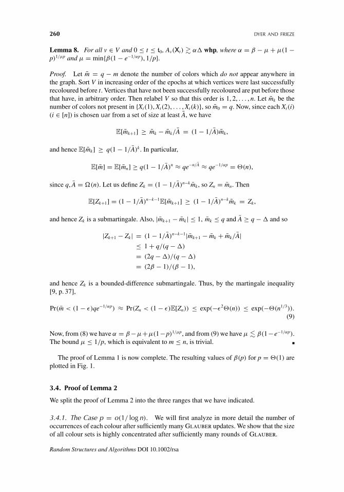
The proof of Lemma 1 is now complete. The resulting values of β(p) for p = �(1) areplotted in Fig. 1.

3.4. Proof of Lemma 2

We split the proof of Lemma 2 into the three ranges that we have indicated.

3.4.1. The Case p = o(1/ log n). We will first analyze in more detail the number ofoccurrences of each colour after sufficiently many Glauber updates. We show that the sizeof all colour sets is highly concentrated after sufficiently many rounds of Glauber.



Fig. 1. Bound on β for convergence of Glauber, using Lemmas 7 and 8.

Lemma 9. Let 0 < ε0 ≤ 1 be a constant and δ0 = n−K for some constant K > 0. Then,with probability at least 1 − δ0, we have sc ≥ (1 − ε0)n/q (∀c ∈ C) for all t1 ≤ t ≤ t0,where

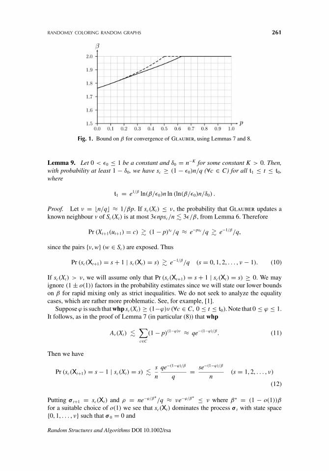
t1 = e1/β ln(β/ε0)n ln (ln(β/ε0)n/δ0) .

Proof. Let ν = �n/q� ≈ 1/βp. If sc(Xt) ≤ ν, the probability that Glauber updates aknown neighbour v of Sc(Xt) is at most 3εnpsc/n � 3ε/β, from Lemma 6. Therefore

Pr (Xt+1(ut+1) = c) � (1 − p)sc/q ≈ e−psc/q � e−1/β/q,

since the pairs {v, w} (w ∈ Sc) are exposed. Thus

Pr (sc(Xt+1) = s + 1 | sc(Xt) = s) � e−1/β/q (s = 0, 1, 2, . . . , ν − 1). (10)

If sc(Xt) > ν, we will assume only that Pr (sc(Xt+1) = s + 1 | sc(Xt) = s) ≥ 0. We mayignore (1 ± o(1)) factors in the probability estimates since we will state our lower boundson β for rapid mixing only as strict inequalities. We do not seek to analyze the equalitycases, which are rather more problematic. See, for example, [1].

Suppose ϕ is such that whp sc(Xt) ≥ (1−ϕ)ν (∀c ∈ C, 0 ≤ t ≤ t0). Note that 0 ≤ ϕ ≤ 1.It follows, as in the proof of Lemma 7 (in particular (8)) that whp

Av(Xt) �∑c∈C

(1 − p)(1−ϕ)ν ≈ qe−(1−ϕ)/β . (11)

Then we have

Pr (sc(Xt+1) = s − 1 | sc(Xt) = s) � s

n

qe−(1−ϕ)/β

q= se−(1−ϕ)/β

n(s = 1, 2, . . . , ν)

(12)

Putting σ t+1 = sc(Xt) and ρ = ne−ϕ/β∗/q ≈ νe−ϕ/β∗ ≤ ν where β∗ = (1 − o(1))β

for a suitable choice of o(1) we see that sc(Xt) dominates the process σ t with state space{0, 1, . . . , ν} such that σ 0 = 0 and


262 DYER AND FRIEZE

Pr (σ t+1 = σ + 1 | σ t = σ) = e−1/β∗

q, (σ = 0, 1, . . . , ν − 1)

Pr (σ t+1 = σ − 1 | σ t = σ) = σe−(1−ϕ)/β∗

n, (σ = 0, 1, . . . , ν)

Pr (σ t+1 = σ | σ t = σ) = 1 − e−1/β∗

q− σe−(1−ϕ)/β∗

n, (σ = 0, 1, . . . , ν − 1)

Pr (σ t+1 = ν | σ t = ν) = 1 − νe−(1−ϕ)/β∗

n.

This is a reversible Markov chain with equilibrium distribution,

Pr(σ∞ = σ) = ρσ e−ρ

ψ σ ! (σ = 0, 1, . . . , ν), ψ =ν∑

σ=0

ρσ e−ρ

σ ! .

as may be verified using the detailed balance equations

e−1/β∗

q

ρσ−1 e−ρ

ψ (σ − 1)! = σe−(1−ϕ)/β∗

n

ρσ e−ρ

ψ σ ! (σ = 1, 2, . . . , ν).

The equilibrium distribution is clearly Poiss(ρ) conditional on σ ≤ ν. If x ∼ Poiss(ρ) andϕ = �(ε), the Chernoff bound gives

Pr(x < (1 − ε)ρ ∨ x > (1 + ε)ρ) ≤ 2 exp

(−1

3ε2ρ

)= exp(−�(ε2ω log n)) ≤ n−θ .

(13)

Thus whp we have

σ∞ ≥ (1 − ε)ρ ≈ ne−ϕ/β∗

q≥

(1 − ϕ

β∗

)n

q. (14)

We may bound the mixing time of the process σ t using path coupling [2]. We considertwo copies xt , yt of the process σ t , where y0 is sampled from the equilibrium distribution.We will use the metric d(xt , yt) = |xt − yt|. We define the coupling on adjacent statesxt = σ − 1, yt = σ (1 ≤ σ ≤ ν), so d(xt , yt) = 1. Conditionally on xt = σ − 1, yt = σ , for0 < σ ≤ ν, we couple the processes as follows

Pr(xt+1 = x, yt+1 = y)

=

(σ − 1)e−(1−ϕ)/β∗

n, if x = σ − 2, y = σ − 1,

1 − σe−(1−ϕ)/β∗

n− e−1/β∗

q, if x = σ − 1, y = σ ,

e−1/β∗

q, if x = σ , y = min{σ + 1, ν},

e−(1−ϕ)/β∗

n, if x = σ − 1, y = σ − 1.



It is now easy to see that

E[d(xt+1, yt+1) | d(xt , yt) = 1] ≤ 1 − e−(1−ϕ)/β∗

n,

and hence

Pr(xt �= yt) ≤ E[d(xt , yt)] ≤ d(x0, y0)

(1 − e−(1−ϕ)/β∗

n

)t

≤ n

q

(1 − e−1/β∗

n

)t

,

from which it follows, using the Coupling Lemma, that for any δ0 we will have

dTV(σ t , σ∞) ≤ n

q

(1 − e−1/β∗

n

)t

≤ n

qexp

(− te−1/β∗

n

)≤ δ0

q,

when t ≥ e1/β∗n ln(n/δ0). Thus, when t ≥ e1/β∗

n ln(n/δ0), we will have sc ≥ (1−ϕ/β∗)n/q(∀c ∈ C) with probability at least 1 − δ0.

We will run this process in k stages. We take ϕ0 = 1, assuming only sc ≥ 0 (∀c ∈ C).For t ≥ e1/β∗

n ln(kn/δ0) we will have sc ≥ (1 −ϕ0/β∗)n/q with probability 1 − δ0/k. Thus

we can take ϕ1 = ϕ0/β∗ and repeat the process. After time t ≥ ke1/β∗

n ln(kn/δ0) we willhave

sc ≥(

1 − ϕ0

(β∗)k

)n

q=

(1 − 1

(β∗)k

)n

q(∀c ∈ C)

with probability 1 − k(δ0/k) = 1 − δ0. So, in time t ≥ e1/β∗ln(β∗/ε0)n ln(ln(β∗/ε0)n/δ0)

≈ e1/β ln(β/ε0)n ln(ln(β/ε0)n/δ0) we will have sc ≥ (1−ε0)n/q (∀c ∈ C) with probabilityat least 1 − δ0.

Corollary 1. For all t1 ≤ t ≤ t0 and v ∈ V, we have

βe−1/β� � Av(Xt) ∼ βe−(1−ε0)/β�, (15)

with probability at least 1 − δ0.

Proof. The left hand inequality follows from Lemma 7. The right hand inequality followsfrom the proof of Lemma 9, in particular (11).

We note here that the better bound on the number of available colors Av(Xt) from Corol-lary 1 can be used to improve the bound on β(p) for p = �(1) using (3)–(5). The resultsare plotted in Fig. 2

We can now verify the upper bound on d∗v in this lemma (see (6) for the definition).

Let v ∈ V , cX = Xt(v) and cY = Yt(v). Also, let SX = ScY (Xt), SY = ScX (Yt) withsX = |SX |, sY = |SY |. From Lemma 3 and Lemma 9 with δ0 = n−10, we know that whp(1 − ε0)n/q ≤ sX , sY ≤ ε2n/ ln n when t ≥ t1. From Lemma 3, we have exposed at mostεnsX pairs adjacent to vertices in SX , εnsY pairs adjacent to vertices in SY , and εn pairsadjacent to v. Let V ′ = V \ (SX ∪ {v}). Then, by simple counting, there can be at mostεn +√

εn +√εn = o(n) vertices w ∈ V ′ such that either the pair {v, w} is exposed, or there

are more than√

εsX = o(n/q) exposed pairs {u, w} (u ∈ SX) or more than√

εsY = o(n/q)

exposed pairs {u, w} (u ∈ SY ). Thus there is a set V ′′ ⊆ V ′, of size ≈ n, such that for w ∈ V ′′,


264 DYER AND FRIEZE

Fig. 2. Bound on β for convergence of Glauber using Corollary 1, also showing the bound fromLemma 8 for comparison.

{v, w} is unexposed and there are ≈ sX unexposed pairs {u, w} (u ∈ SX) and ≈ sY unexposedpairs {u, w} (u ∈ SY ). Hence, for w ∈ V ′′,

Pr(w ∈ N ∗v ) � p

((1 − p)sX + (1 − p)sY − (1 − p)sX +sY −|SX ∩SY |) (16)

≤ p((1 − p)sX + (1 − p)sY − (1 − p)sX +sY

)= p (1 − (1 − (1 − p)sX )(1 − (1 − p)sY )) (17)

≤ p(1 − (1 − (1 − p)(1−ε0)n/q)2

)� p

(1 − (1 − e−(1−ε0)/β)2

).

Moreover, these bounding events are independent for all w ∈ V ′′. Let γ = 1 − (1 −e−(1−ε0)/β)2. Then, using the Chernoff bound,

Pr(d∗

v > (1 + ε)γ�) ≤ exp(−�(ε2�)) = n−θ . (18)

This completes the proof of Lemma 2 and Theorem 1 for this case.

3.4.2. The Case p = o(1), p = �(1/ log n).

Lemma 10. Let 0 < ε0, δ0 ≤ 1 be constants. Then, with probability at least 1 − δ0, wehave that for all t1 ≤ t ≤ t0, sc ≥ (1 − ε0)n/q for almost all c ∈ C, where

t1 = e1/β ln(β/ε0)n ln(

ln(β/ε0)n/δ0

).

Proof. When p = �(1/ log n), the analysis of Section 3.4.1 fails, even for p = o(1).The equilibrium distributions of individual sc(Xt) are not sufficiently concentrated even toprove Corollary 1 directly. However, conditional on the sc (c ∈ C), we may still proveconcentration of Av(Xt) as in Lemma 7. We may then prove Corollary 1 as follows.

We combine the q = �(n/ log n) colors into � ≈ q/r groups, C1, C2, . . . , C�, each ofsize r = �ω ln n or r +1. Consider a particular group Cj. For c ∈ Cj, we may bound sc by arandom process σ t , as in section 3.4.1. Moreover, the processes are close to being indepen-dent for all c ∈ Cj. This follows from the facts that q = �(n/ log n), and sc ≤ ε4 ln2 n, from



Lemma 3, so∑

c∈Cjsc = o(log3 n) whp. Using this, we can bound the transition probabil-

ities of each sc (c ∈ Cj) conditionally on the rest, and show independence to a sufficientlyclose approximation. More precisely we can replace (10) and (12) by

Pr(sc(Xt+1) = s + 1 | sc(Xt) = s, sc′ , c′ ∈ Cj \ {c}) � e−1/β/q (0 ≤ s < ν). (19)

Pr(sc(Xt+1) = s − 1 | sc(Xt) = s, sc′ , c′ ∈ Cj \ {c}) � se−(1−ϕ)/β

n(1 ≤ s ≤ ν) (20)

Then the argument for a given sc follows the proof of Lemma 9, using the process definedthere, so we will simply indicate the differences.

The value of ρ is not large enough to get the RHS of (13). Instead, all we can say is thatfor x ∼ Poiss(ρ),

Pr(x < (1 − ϕ)ρ) ≤ εϕ = exp

(−1

2ϕ2ρ

)= o(1).

So we weaken the hypothesis sc(Xt) ≥ (1 − ϕ)ν to

Pr(sc(Xt) < (1 − ϕ)ν) < εϕ (∀c ∈ C, 0 ≤ t ≤ t0).

(This is enough to prove the lemma. The value of ϕ tends to zero as we iterate.) Note thatthen

E[(1 − p)sc(Xt )] ≤ (1 − p)(1−ϕ)ν + εϕ ≤ e−(1−ϕ)/β + εϕ ≈ e−(1−ϕ)/β ,

and hence

E[Av(Xt)] ∼ qe−(1−ϕ)/β ≈ �re−(1−ϕ)/β .

However, to show that (11) remains true, we must prove concentration. Now 0 ≤ (1−p)sc ≤1, and E[(1 − p)sc ] ∼ e−(1−ϕ)/β , so we may use Hoeffding’s inequality [8] to show that

Pr

∑

c∈Cj

(1 − p)sc ≥ (1 + ε)re−(1−ϕ)/β

∼ exp

(−�(ε2ω log n)) = n−θ ,

and hence

Pr

(∑c∈C

(1 − p)sc ≥ (1 + ε)qe−(1−ϕ)/β

)≤ n−θ .

This shows that the required upper bound (11) for Av(Xt) holds whp. The remainder ofthe proof now follows that of Lemma 9, except that (14) can be proved to hold only withprobability 1 − εϕ . However, this is the inductive hypothesis, so we may conclude thatCorollary 1 holds for all p = o(1).

When p = �(1/ log n), the bound (18) is not valid. However, observe that we onlyrequire the bound on d∗

v to hold in expectation. We must deal with conditioning on d∗v ,

but only by the event v ∈ W , not by the whole of W . Therefore, we need to estimateE[d∗

v | v ∈ W] at a given time t∗. To do this, we must bound the random variable sc(Xt∗)


266 DYER AND FRIEZE

conditional on Xt∗(v) = c and v ∈ W . Since we cannot ignore the conditioning here, theapproach must be different from that of Section 3.4.1.

If v ∈ W , then at time tv < t∗, the last successful update of v occurred either in Xtv orYtv . Thus u = v, cX = Xtv(v), cY = Ytv(v), and cX �= cY . We have Xt(v) = cX , Yt(v) = cY

for all tv < t ≤ t∗. We wish to bound sX = scY (X) and sY = scX (Y) from below [see (16)].But the evolution of sX during (tv, t∗) is independent of Xt(v), since Xt(v) = cX throughout.Similarly the evolution of sY during (tv, t) is independent of Yt(v).

We assume that t ≥ t1, so the process has been running long enough that the inequalityin Corollary 1 is true, with the claimed probability. Consequently, Av(Xt) and Av(Yt) areboth close to βe−1/β� for all v and t ≤ t0. The construction of Couple implies that theprobability that an update of v is successful in X but unsuccessful in Y is at most 3ε0 say. Fora given v ∈ W , let tv be the last epoch before t∗ at which a successful update of v occurredin X, and let T = t∗ − tv. Let AL, AR denote the quantities on LHS and RHS of (15). LetρL = n/AL and ρR = n/AR. Then the (conditional) probability of a successful update at vis at least AL

nq = 1ρLq and so the distribution of T satisfies

Pr(T ≥ t) ≤(

1 − 1

ρLq

)t

(t = 0, 1, . . . , t∗) (21)

Let b = β/(β − 1) and assume t∗ ≥ t2 = t1 + 4bn ln n. Now AL ≥ (q − �) and so1/ρLq ≥ 1/bn. So Pr(T > 4bn ln n) ≤ (1 − 1/bn)4bn ln n < n−4. Thus we can take tv ≥ t1

for all v ∈ V and t2 ≤ T ≤ t0 with probability 1 − o(1/n).

Analysis of a bounding process. We now consider two copies of a bounding process thatwill be dominated by the processes sX , sY . The processes can be assumed independent, asdiscussed in (19) and (20).

We consider the process

Pr(σ t+1 = σ + 1 | σ t = σ) = (1 − p)σ

q(σ = 0, 1, 2, . . .) (22)

Pr(σ t+1 = σ − 1 | σ t = σ) = σ

n

A

q= σ

qρ(σ = 0, 1, 2, . . .), (23)

where A is a uniform upper bound on Av(Xt) (v ∈ V , t1 ≤ t ≤ t0), and ρ = n/A. FromLemma 7, we know that A � βnp(1 − p)1/βp, so ρ = O(1) when p = �(1).

Thus, if we assume sX = sY = 0 at time tv, we can bound sX and sY at time t∗ bytwo independent processes of the form (22)–(23) during (tv, t∗). In particular we wish toexamine the transient behaviour of σ t , with this distribution and ρ = ne1/β/q.

(Of course, we can only assume a ρ which fluctuates close to this value, but simple bound-ing arguments justify the use of this particular value). In particular, we wish to determinecertain properties of σ T at a random time T such that

Pr(T ≥ t) =(

1 − 1

ρq

)t

(t = 0, 1, 2, . . .).

Now

E[σ t+1] = σt + (1 − p)σt

q− σt

qρ.



Putting ψt = pσt we may rewrite this as

E[ψt+1 − ψt]p

= e−γψt

βnp− ψte−1/β

βnp.

Here e−γ ≈ (1 − p)1/p ≈ 1/e and the error in putting q = np will be absorbed into γ whichis close to 1.

Let x = βψt and z = e−1/β t/n so that

E[x(z + e−1/β/n) − x(z)]βp

= e−γ x(z)/β

βnp− x(z)e−1/β

βnp. (24)

Using the proof idea of Theorem 5.1 of Wormald [15] we see that (24) is closelyapproximated by the differential equation

dx

dz= e(1−x)/β − x, so z(x) =

∫ x

0

dy

e(1−y)/β − y(0 ≤ x < 1).

The upper bound x < 1 is due to the fact that dx/dz = 0 when x = 1, the lower boundx ≥ 0 to the assumption σ0 = 0.

Let σ t , σ ′t be iid processes with the distribution (22)–(23). We wish to determine (see

(17))

E[(1 − (1 − p)σ t )(1 − (1 − p)σ ′t )] ≈ E[1 − e−pσ t ]E[1 − e−pσ ′

t ]= E[1 − e−pσ t ]2 ≈ (1 − e−x(z)/β)2

at the random epoch t = T , where T has the distribution Pr(T ≥ t) ≈ (1−e−1/β/n)t ≈ e−z.Hence, using parts integration,

E[(1 − (1 − p)σT)2] =∫ ∞

0(1 − e−x(z)/β)2e−z dz

=∫ 1

0(1 − e−x/β)2e−z(x) dz

dxdx

= [−(1 − e−x/β)2e−z(x)]1

0+ 2

β

∫ 1

0(1 − e−x/β)e−z(x) dx

= 2

β

∫ 1

0(1 − e−x/β) exp

(− x

β−

∫ x

0

dy

e(1−y)/β − y

)dx. (25)

Thus we can write

Pr(w ∈ N ∗v | v ∈ W) ≤ κ1(β) + δ0 + 3ε0.

This completes our upper estimate E[d∗v | v ∈ W] required for Lemma 2 and so completes

the proof of Theorem 1 for this case.

3.4.3. The Case p = �(1). By detailed balance, the equilibrium distribution σ∞ of(22)–(23) is given by

Pr(σ∞ = σ) = ρσ (1 − p)σ(σ−1)/2

G(ρ)σ ! (σ = 0, 1, 2, . . .), (26)


268 DYER AND FRIEZE

where G(ρ) = ∑∞σ=0 ρσ (1 − p)σ(σ−1)/2/σ !, since

(1 − p)σ−1

q

ρσ−1(1 − p)(σ−1)(σ−2)/2

(σ − 1)! = σ

ρq

ρσ (1 − p)σ(σ−1)/2

σ ! (σ = 1, 2, . . .).

We will denote a random variable with the distribution given in (26) by σ∞(ρ).We can bound the mixing time of the process σ t using path coupling. We define the

coupling on adjacent states xt = σ − 1, yt = σ (σ > 0) as follows

Pr(xt+1 = x, yt+1 = y) =

σ − 1

ρq, if x = σ − 2, y = σ − 1,

(1 − p)σ

q, if x = σ , y = σ + 1,

1

ρq, if x = σ − 1, y = σ − 1,

p(1 − p)σ−1

q, if x = σ , y = σ ,

1 − σ

ρq− (1 − p)σ−1

qif x = σ − 1, y = σ .

It is now easy to see that

E[d(xt+1, yt+1) | d(xt , yt) = 1] ≤ 1 − 1

ρq− p(1 − p)xt

q< 1 − 1

ρq. (27)

Since ρ = O(1) and q = O(n) in (27), convergence occurs in O(n log n) time.We may now use the proof method from Section 3.4.2 to show that, for all t1 ≤ t ≤ t0

and v ∈ V , whp we have

Av(Xt) �∑c∈C

E[(1 − p)sc(Xt )] ≈ qE[(1 − p)sc(Xt )],

by symmetry. Hence we may take A0 = n/ρ0, ρ0 = n/q, corresponding to Av(Xt) ≤ q, andthen we will obtain whp

Av(Xt) � A1 ≈ qE[(1 − p)σ∞(ρ0)].

As in Section 3.4.1, we may run this process iteratively. The iteration is analyzed below andis shown to converge in O(1) steps so that whp

Av(Xt) � A∗ = qE[(1 − p)σ∞(ρ∗)] = qE[σ∞(ρ∗)]ρ∗ = n

ρ∗ ≈ �

pρ∗ ,

where ρ∗ is the solution to

E[σ∞(ρ∗)] = n

q≈ 1

βpor β ≈ 1

pE[σ∞(ρ∗). (28)



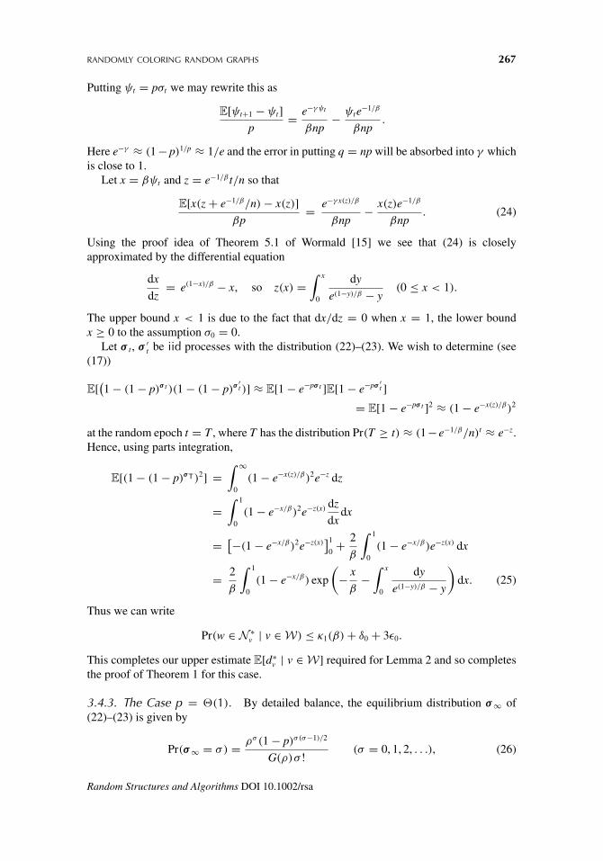
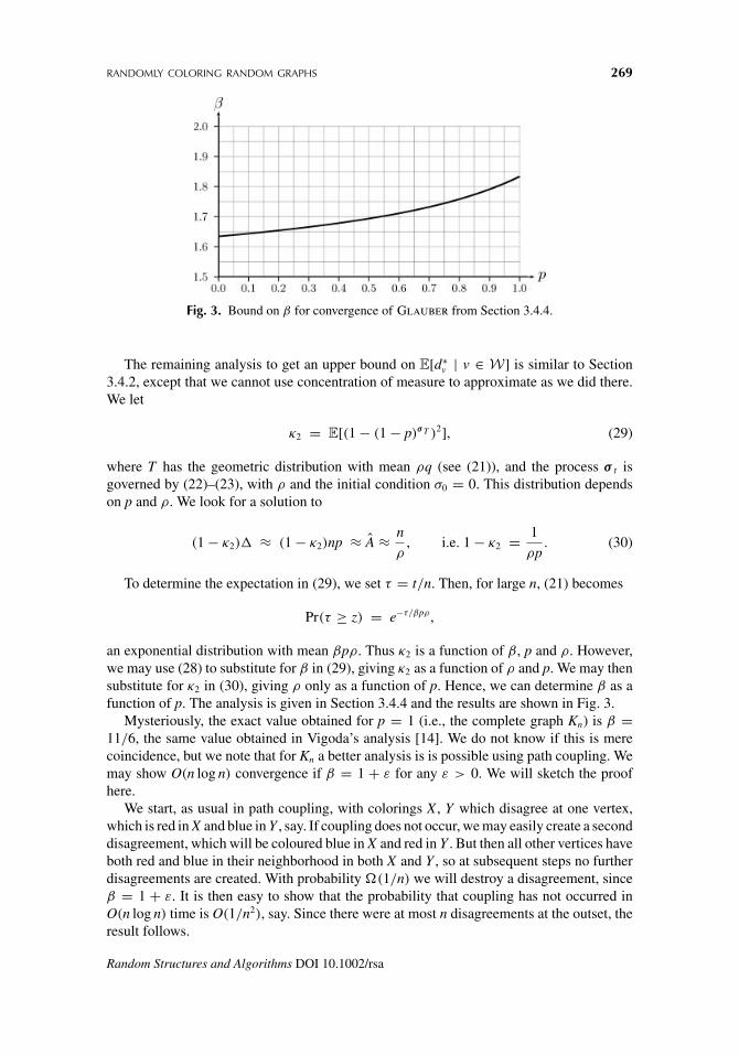
Fig. 3. Bound on β for convergence of Glauber from Section 3.4.4.

The remaining analysis to get an upper bound on E[d∗v | v ∈ W] is similar to Section

3.4.2, except that we cannot use concentration of measure to approximate as we did there.We let

κ2 = E[(1 − (1 − p)σT )2], (29)

where T has the geometric distribution with mean ρq (see (21)), and the process σ t isgoverned by (22)–(23), with ρ and the initial condition σ0 = 0. This distribution dependson p and ρ. We look for a solution to

(1 − κ2)� ≈ (1 − κ2)np ≈ A ≈ n

ρ, i.e. 1 − κ2 = 1

ρp. (30)

To determine the expectation in (29), we set τ = t/n. Then, for large n, (21) becomes

Pr(τ ≥ z) = e−τ/βpρ ,

an exponential distribution with mean βpρ. Thus κ2 is a function of β, p and ρ. However,we may use (28) to substitute for β in (29), giving κ2 as a function of ρ and p. We may thensubstitute for κ2 in (30), giving ρ only as a function of p. Hence, we can determine β as afunction of p. The analysis is given in Section 3.4.4 and the results are shown in Fig. 3.

Mysteriously, the exact value obtained for p = 1 (i.e., the complete graph Kn) is β =11/6, the same value obtained in Vigoda’s analysis [14]. We do not know if this is merecoincidence, but we note that for Kn a better analysis is is possible using path coupling. Wemay show O(n log n) convergence if β = 1 + ε for any ε > 0. We will sketch the proofhere.

We start, as usual in path coupling, with colorings X, Y which disagree at one vertex,which is red in X and blue in Y , say. If coupling does not occur, we may easily create a seconddisagreement, which will be coloured blue in X and red in Y . But then all other vertices haveboth red and blue in their neighborhood in both X and Y , so at subsequent steps no furtherdisagreements are created. With probability �(1/n) we will destroy a disagreement, sinceβ = 1 + ε. It is then easy to show that the probability that coupling has not occurred inO(n log n) time is O(1/n2), say. Since there were at most n disagreements at the outset, theresult follows.


270 DYER AND FRIEZE

Analysis of a bounding process. Let G(ρ) = ∑∞σ=0 ρσ (1−p)σ(σ−1)/2/σ !. Note that 1+ρ ≤

G(ρ) ≤ eρ . We consider a random variable σ = σ∞ such that

Pr(σ = σ) = ρσ (1 − p)σ(σ−1)/2

G(ρ)σ ! (σ = 0, 1, 2, . . .).

We consider ρ to be a parameter, so we will write, for example, E[σ (ρ)] if we wish to specifythe parameter. If the parameter is not specified, its value is ρ. Thus E[σ ] = E[σ (ρ)]. Wewill also write ρ = ez and g(z) = G(ez). Let us write p = (1 − p). Then easy calculationsshow that

G′(ρ) = G(ρ)E[σ ]/ρ = G((1 − p)ρ) = G(ρ)E[(1 − p)σ ], (31)

G′′(ρ) = G(ρ)E[σ (σ − 1)]/ρ2 = (1 − p)G′((1 − p)ρ), (32)

g′(z) = g(z)E[σ ], g′′(z) = g(z)E[σ 2]. (33)

We first show that E[σ ] is a strictly increasing function of z.

dE[σ ]dz

= d

dz

(g′(z)g(z)

)= g(z)g′′(z) − g′(z)2

g(z)2= E[σ 2] − E[σ ]2 = Var[σ ] > 0. (34)

We wish to analyze the iteration

ρ0 = n

q, ρi+1 = n

qE[(1 − p)σ (ρi)] = nρi

qE[σ (ρi)] = nezi g(zi)

qg′(zi)(i ≥ 0),

using (31). Taking logarithms, and using (33), we consider instead the equivalent iteration,

z0 = ln(n/q), zi+1 = f (zi) = zi + ln(n/q) + ln g(zi) − ln g′(zi) (i ≥ 0). (35)

Now, using (31)–(34), we have

f ′(z) = 1 + g′(z)g(z)

− g′′(z)g′(z)

= 1 + E[σ ] − E[σ 2]E[σ ] = 1 − Var[σ ]

E[σ ] (36)

= E[σ ] − E[σ (σ − 1)]E[σ ] = ρ

G′(ρ)

G(ρ)− (1 − p)ρ

G′((1 − p)ρ)

G((1 − p)ρ

)= E[σ (ρ)] − E[σ ((1 − p)ρ)]. (37)

From (36) and (37) we see that 0 < f ′(z) < 1 for all z ∈ R.Consider the equation z = f (z). This is equivalent to E[σ (ρ)] = n/q from (33) and (35),

so it has at most one root because E[σ ] is strictly increasing. It is also easy to show that ithas a root, since (31) and Jensen’s inequality imply

ρ(1 − p)E[σ ] ≤ ρE[(1 − p)σ ] = ρG′(ρ)

G(ρ)= E[σ ] ≤ ρ (using G′(ρ) ≤ G(ρ) − − (31))

From the right inequality, we have E[σ (ρ0)] ≤ ρ0 = n/q. From the left, we see thatE[σ ] > (1 − p) ln ρ. Otherwise, since x ≥ −(1 − x) ln(1 − x) (0 ≤ x ≤ 1) and x > ln x(x > 0), we would have

E[σ ] ≥ ρ(1 − p)(1−p) ln ρ = ρ1+(1−p) ln(1−p) ≥ ρ1−p > ln ρ1−p = (1 − p) ln ρ, (38)

a contradiction. Hence E[σ (ρ)] > n/q for large enough ρ.



We may use (36) and (38) to give an explicit upper bound on f ′(z), as follows.

1 − f ′(z) = Var[σ ]E[σ ] ≥ E[σ ]2 Pr(σ = 0)

E[σ ] = E[σ ]G(ρ)

≥ (1 − p)e−ρ ln ρ.

Let z∗ be the root of z = f (z), and ρ∗ = ez∗ . Now we have

z0 = ln(n/q) = ln E[σ (ρ∗)] ≤ ln ρ∗ = z∗

and

z∗ = ln ρ∗ ≤ E[σ (ρ∗)]1 − p

= n

q(1 − p)≈ 1

βp(1 − p)

If zi < z∗ then, for some zi with zi ≤ zi ≤ z∗,

zi+1 = f (zi) = f (z∗ + (zi − z∗)) = f (z∗) + (zi − z∗)f ′(zi) = z∗ − (z∗ − zi)f′(zi) < z∗,

Thus {zi} is a bounded increasing sequence, so convergent. More precisely, we have

f ′(zi) � 1 − (1 − p)e−ρ ln ρ = 1 − ϕ,

where ρ = exp( 1βp(1−p)

) and ϕ = (1 − p)e−ρ ln ρ. Therefore

z∗ − zi+1 = (z∗ − zi)f′(zi) < (z∗ − zi)(1 − ϕ) ≤ (z∗ − z0)(1 − ϕ)i � e−iϕ

βp(1 − p).

Thus we have z∗ − ε0 < zi < z∗ when i ≥ i∗ = �ϕ ln(βp(1 − p)ε0) = O(1).

3.4.4. Final Analysis. Let Hσ (t) = Pr(σ t = σ). Note that H0(0) = δσ , where δ0 = 1and δσ = 0 for all σ > 0. Then, using (22)–(23),

Hσ (t + 1) = (1 − p)σ−1

qHσ−1(t) +

(1 − (1 − p)σ

q− σ

ρq

)Hσ (t) + σ + 1

ρqHσ+1(t),

where ρ is the solution to E[σ (ρ)] = 1/βp, using the distribution of (26). Thus

ρq(Hσ (t + 1) − Hσ (t)) = ρ(1 − p)σ−1Hσ−1(t)− (ρ(1 − p)σ + σ)Hσ (t) +(σ +1)Hσ+1(t).

Let τ = t/n. Then, as n → ∞, this becomes

βpρH ′σ (τ ) = ρ(1 − p)σ−1Hσ−1(τ ) − (ρ(1 − p)σ + σ)Hσ (τ ) + (σ + 1)Hσ+1(τ ), (39)

with the initial conditions H0(0) = 1, H0(τ ) = 0 (τ > 0). Differentiating this gives

βpρH ′′σ (τ ) = ρ(1 − p)σ−1H ′

σ−1(τ ) − (ρ(1 − p)σ + σ)H ′σ (τ ) + (σ + 1)H ′

σ+1(τ ), (40)

with the initial conditions H ′0(0) = −ρ, H ′

0(1) = ρ, H ′0(τ ) = 0 (τ > 0). We used (39) and

(40) as the basis of a second-order method for approximating Hσ (τ ) at sufficiently manyvalues of τ . Hence we could estimate F(τ ) = E[(1 − p)στ ].

Now Pr(T ≥ nτ) ≈ (1 − 1/ρq)nτ ≈ e−ητ , where 1/η = βρp so we could estimate

κ2 =∫ ∞

0(1 − F(τ ))2e−ητ ηdτ , (41)

and hence solve (30) for ρ. Then β could be calculated from (28). This was used to obtainβ(p) to five decimal places for all values of p from 0 to 1 in steps of 0.025. The results areplotted in Fig. 3.


272 DYER AND FRIEZE

REFERENCES

[1] M. Bordewich and M. Dyer, Path coupling without contraction, J Discrete Algorithms 5 (2007),280–292.

[2] R. Bubley and M. Dyer, Path coupling: A technique for proving rapid mixing in Markovchains, Proceedings 38th, Annual IEEE Symposium on Foundations of Computer Science,IEEE Computer Society, Washington, DC, 1997, pp. 223–231.

[3] M. Dyer, A. Flaxman, A. Frieze, and E. Vigoda, Randomly coloring sparse random graphswith fewer colors than the maximum degree, Random Struct Algorithms 29 (2006), 450–465.

[4] M. Dyer and A. Frieze, Randomly coloring graphs with lower bounds on girth and maximumdegree, Random Struct Algorithms 23 (2003), 167–179.

[5] A. Frieze and E. Vigoda, A survey on the use of Markov chains to randomly sample colorings,In G. Grimmett and C. McDiarmid, editors, Combinatorics, complexity and chance, a tributeto dominic Welsh, Oxford University Press, Oxford, England, 2007, pp. 53–71.

[6] G. Hardy, J. Littlewood, and G. Pólya, Inequalities, 2nd edition, Cambridge University Press,Cambridge, 1988.

[7] T. Hayes and E. Vigoda, Coupling with the stationary distribution and improved samplingfor colorings and independent sets, In Proceedings 16th Annual ACM-SIAM Symposium onDiscrete Algorithms, SIAM Press, Philadelphia, 2005, pp. 971–979.

[8] W. Hoeffding, Probability inequalities for sums of bounded random variables, J Am Stat Assoc58 (1963), 13–30.

[9] S. Janson, T. Łuczak, and A. Rucinski, Random graphs, Wiley-Interscience, New York, 2000.

[10] M. Jerrum, A very simple algorithm for estimating the number of k-colorings of a low-degreegraph, Random Struct Algorithms 7 (1995), 157–165.

[11] M. Jerrum, Counting, sampling and integrating: Algorithms and complexity, ETH ZürichLectures in Mathematics, Birkhäuser, Basel, 2003.

[12] M. Molloy, The Glauber dynamics on colorings of a graph with high girth and maximumdegree, SIAM J Comput 33 (2004), 721–737.

[13] E. Mossell and A. Sly, Gibbs rapidly samples colorings of G(n, d/n), to appear in Probabilityand Related Fields.

[14] E. Vigoda, Improved bounds for sampling colorings, J Math Phys 41 (2000), 1555–1569.

[15] N. Wormald, The differential equation method for random graph processes and greedy algo-rithms, In M. Karonski and H. J. Prömel, editors, Lectures on approximation and randomizedalgorithms, PWN, Warsaw, 1999, pp. 73–155.


Documents

Randomly coloring random graphs