Embed Size (px)
Citation preview
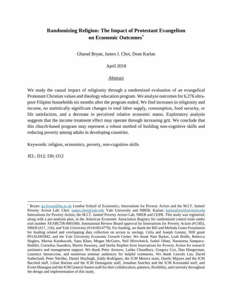
Randomizing Religion: The Impact of Protestant Evangelism
on Economic Outcomes*
Gharad Bryan, James J. Choi, Dean Karlan
April 2018
Abstract
We study the causal impact of religiosity through a randomized evaluation of an evangelical
Protestant Christian values and theology education program. We analyze outcomes for 6,276 ultra-
poor Filipino households six months after the program ended. We find increases in religiosity and
income, no statistically significant changes in total labor supply, consumption, food security, or
life satisfaction, and a decrease in perceived relative economic status. Exploratory analysis
suggests that the income treatment effect may operate through increasing grit. We conclude that
this church-based program may represent a robust method of building non-cognitive skills and
reducing poverty among adults in developing countries.
Keywords: religion, economics, poverty, non-cognitive skills
JEL: D12; I30; O12
* Bryan: [email protected] London School of Economics, Innovations for Poverty Action and the M.I.T. Jameel
Poverty Action Lab; Choi: [email protected] Yale University and NBER; Karlan: [email protected]
Innovations for Poverty Action, the M.I.T. Jameel Poverty Action Lab, NBER and CEPR. This study was registered,
along with a pre-analysis plan, in the American Economic Association Registry for randomized control trials under
trial number AEARCTR-0001060. Institutional Review Board approval by Innovations for Poverty Action (#1185),
NBER (#17_116), and Yale University (#1410014779). For funding, we thank the Bill and Melinda Gates Foundation
for funding related and overlapping data collection on access to savings, Celia and Joseph Grenny, NIH grant
P01AG005842, and the Yale University Economic Growth Center. We thank Nate Barker, Leah Bridle, Rebecca
Hughes, Marius Karabaczek, Sana Khan, Megan McGuire, Neil Mirochnick, Isabel Oñate, Nassreena Sampaco-
Baddiri, Cornelius Saunders, Martin Sweeney, and Sneha Stephen from Innovations for Poverty Action for research
assistance and management support. We thank Peter Aronow, Latika Chaudhary, Gregory Cox, Dan Hungerman,
Laurence Iannaccone, and numerous seminar audiences for helpful comments. We thank Lincoln Lau, David
Sutherland, Peter Nitchke, Daniel Mayhugh, Zaldy Rodriguez, the ICM Metrics team, Danilo Mijares and the ICM
Bacolod staff, Lilian Barinas and the ICM Dumaguete staff, Jonathan Sanchez and the ICM Koronadal staff, and
Evren Managua and the ICM General Santos staff for their collaboration, patience, flexibility, and curiosity throughout
the design and implementation of this study.

2
A literature dating back at least to Adam Smith and Max Weber finds that religiosity is
associated with a set of characteristics that promote economic success, including diligence,
thriftiness, trust, and cooperation (Iannaccone 1998; Iyer 2016). More recent research has linked
religiosity to positive outcomes in domains such as physical health (Ellison 1991), crime rates
(Freeman 1986), drug and alcohol use (Gruber and Hungerman 2008), income (Gruber 2005), and
educational attainment (Freeman 1986; Gruber 2005). However, demonstrating that religion
causes outcomes is challenging because people choose their religion. Naturally occurring religious
affiliation is likely to be correlated with unobserved personal characteristics that may be the true
drivers of the observed correlations. Iannaccone (1998) writes that “nothing short of a (probably
unattainable) ‘genuine experiment’ will suffice to demonstrate religion’s causal impact.”2
To study the causal impact of religiosity, we partnered with International Care Ministries
(ICM), an evangelical Protestant anti-poverty organization that operates in the Philippines, to
conduct an evaluation that randomly assigned invitations to attend Christian theology and values
training. There are 285 million evangelical Christians in the world, comprising 13% of Christians
and 36% of Protestants (Hackett and Grim 2011).3 ICM is representative of an important sector
that attempts to generate religiosity while alleviating poverty.
ICM’s program, called Transform, normally consists of three components—Protestant
Christian theology, values, and character virtues (“V”), health behaviors (“H”), and livelihood
(i.e., self-employment) skills (“L”)—taught over 15 weekly meetings (plus a 16th meeting for a
graduation ceremony). Each meeting lasts 90 minutes, spending 30 minutes per component. ICM’s
leadership believes that the V curriculum lies firmly in the mainstream of evangelical belief. Since
2009, 194,000 people have participated in Transform. The basic structure of the program, using a
set series of classes outside of a Sunday worship service to evangelize, is a common model. For
example, over 24 million people in 169 countries have taken the evangelistic Alpha course since
2 A notable example of a natural experiment is Clingingsmith, Khwaja, and Kremer (2009), who study a randomized
lottery in Pakistan for participation in the hajj. Laboratory experiments that study religious effects by exogenously
varying the salience of religion include Shariff and Norenzyan (2007), Mazar, Amir, and Ariely (2008), Hilary and
Hui (2009), Horton, Rand, and Zeckhauser (2011), and Benjamin, Choi, and Fisher (2016). See Shariff et al. (2016)for
a review of the laboratory literature. 3 The National Association of Evangelicals lists four defining characteristics of evangelical Christians that have been
identified by historian David Bebbington: “the belief that lives need to be transformed through a ‘born-again’
experience and a life long process of following Jesus,” “the expression and demonstration of the gospel in missionary
and social reform efforts,” “a high regard for and obedience to the Bible as the ultimate authority,” and “a stress on
the sacrifice of Jesus Christ on the cross as making possible the redemption of humanity.” (https://www.nae.net/what-
is-an-evangelical/, accessed April 20, 2018)

3
1977 (Bell 2013), and Samaritan’s Purse has enrolled 11 million children in about 100 countries
in its evangelistic Greatest Journey course since 2010 (Samaritan’s Purse 2017). Like Transform,
these are courses of approximately a dozen sessions.
We randomly assigned communities to receive the full Transform curriculum (VHL), to
receive only the health and livelihoods components of the curriculum (HL), to receive only the
values component of the curriculum (V), or to be a no-curriculum control (C). We identify the
effect of religiosity by the comparison of invited households in VHL communities to invited
households in HL communities, and invited households in V communities to households in C
communities that would have been invited had that community been assigned to be treated.
Religiosity is not a singular concept, and its causal impact will likely depend on many factors.
An important distinction is noted by Johnson, Tompkin, and Webb (2008), who differentiate
between “organic” exposure to religion over a prolonged period of time (e.g., through one’s
upbringing at home) and “intentional” exposure through participation in a specific program
targeting a specific set of individuals. Both are important channels of religious propagation, and
the type of religiosity produced may depend on the channel. Our study is about intentionally
generated religiosity4 of a specific kind (evangelical Protestant Christian), and a significant aim of
our study is to establish, in the context of a randomized controlled trial, that intentional exposure
to a religious program can generate the critical first stage: an exogenous change in religiosity.
We measure outcomes approximately six months after the training sessions ended and analyze
them in accordance with a pre-analysis plan. We find that those who were invited to receive the
values curriculum have significantly higher religiosity than those who did not receive the values
curriculum, demonstrating that the treatment had its intended first-stage effect. Examining
downstream economic outcomes while correcting for multiple hypothesis tests, we find that the
values curriculum increased household income, but it had no statistically significant effect on total
labor supply, assets, consumption of a subset of goods, food security, or life satisfaction, and it
decreased perceptions of relative economic status within one’s community.5 Post-hoc analysis on
the health and livelihoods curriculum finds that it had no significant treatment effects on income
and perceived relative economic status; this serves as a placebo test that strengthens the case that
4 Gruber and Hungerman (2008), Gruber (2005), and Bottan and Perez-Truglia (2015), who use naturally occurring
shocks to religious participation, are likely estimating the effect of organic exposure to religion. 5 Although we find no significant increase in consumption, the confidence intervals are such that we cannot reject the
hypothesis that the entire increase in income is consumed.

4
the values curriculum treatment effects are operating through religiosity rather than some other
mechanism associated with attending classes run by ICM. Additional post-hoc analysis shows that
the income effect is strongly concentrated on the Transform invitee and is not significant for other
household members’ labor income, suggesting that the estimated income effect is not a Type I
error.
Exploratory regressions suggest that the religiosity treatment effect operates by increasing
grit—specifically, the portion of grit associated with perseverance of effort. We find no consistent
movement in the other potential mechanisms that we measured: social capital, locus of control
(other than the belief that God is in control, which increases), optimism, and self-control.
Our paper is related to a recent literature that argues that non-cognitive skills are important
drivers of economic outcomes and can be improved through specific interventions (Duckworth et
al. 2007; Kautz et al. 2014; Blattman, Jamison, and Sheridan 2015). This body of work raises the
possibility that programs to improve non-cognitive skills might have large positive impacts on the
lives of the most disadvantaged people, but three obstacles need to be overcome to meet this goal.
First, with a few exceptions (e.g., Blattman, Jamison, and Sheridan 2015), existing studies
concentrate on developed countries, while most of the world’s poorest people live in the
developing world. Even if we can assume that non-cognitive skills are similarly malleable in the
developing world, it is not clear that the environment and market structures allow for economic
gains. Second, much of the literature concentrates on children, and little is known about the ability
to improve the non-cognitive skills of adults, although Kautz et al. (2014) notes that non-cognitive
skills are more malleable later in life than cognitive skills. Finally, it is unclear whether
interventions that create large improvements can be delivered in a cost-effective, scalable manner.
Our results suggest that church-based programs might be a solution. Church-based programs make
use of a large existing infrastructure, teach a well-understood and developed set of values, and are
often low cost because they leverage the intrinsic motivation of church members.
I. The ICM Transform Program
Transform’s Values curriculum begins by teaching participants to recognize the goodness of
the material world and their own high worth as God’s creation. The theme then shifts towards
humanity’s rebellion against God and its negative consequences, while contrasting that with the
message that “believers of Jesus will discover joy in sorrow, strength in weakness, timely provision

5
in time of poverty, and peace in the midst of problems and pain.” (Transform does not, however,
teach prosperity theology—the belief that following God will guarantee economic prosperity and
physical health.6) The Protestant doctrine of salvation by grace—a person cannot earn her way into
heaven by performing good works, but can only be saved by putting her faith in Jesus, upon which
God forgives her sins as a free act of grace—is taught. The proper response to God’s grace is to
do good works out of gratitude. The final section of the curriculum covers what such good works
would be. They include stopping wasting money on gambling and drinking, saving money, treating
everyday work as “a sacred ministry,” and becoming active in a local church community.
Participants are encouraged to find hope in the midst of disasters through faith and generally see
that “life’s trials and troubles” are “God’s pruning knife” that will result in “more fruitfulness.”
In other words, the curriculum teaches students that their suffering has meaning and purpose, and
aims to build the ability to persevere through setbacks. These curricular elements dovetail with the
growing literature on non-cognitive skills that emphasizes the importance of characteristics like
conscientiousness, grit, resilience to adversity, self-esteem, and the ability to engage productively
in society (Kautz et al. 2014)..
The Health training focuses on building health knowledge and changing health and hygiene
practices in the household. Additionally, ICM staff identify participants experiencing
malnourishment and common health issues such as diarrhea, tuberculosis, and skin problems. They
then receive nutritional supplements, deworming pills, other medical treatments, and follow-up
care.
The Livelihood section of the program consists of training in small business management
skills, training in one of several different livelihood options (for example, an introduction to
producing compost through vermiculture), and being invited to a savings group. Minor agricultural
assistance is given in the form of small seed kits. These activities are intended to provide key tools
for achieving a more sustainable income and smoothing economic shocks.
The health and livelihoods components are led by two employees of ICM, while the religious
training is led by a local pastor following an ICM-provided curriculum. The local pastor is not
compensated by ICM but does receive training and support. Six lay volunteers from the pastor’s
6 The teacher’s manual for the Values curriculum says that “we also see ordinary and simple people who enthrone
God as their Lord and Savior discover the deep satisfaction and contentment that make them happy even in their
relative poverty.”
6
church serve as counselors who offer support and encouragement to the participants. For a small
number of participants, ICM arranges treatment for serious medical needs.
The teacher’s manuals used by ICM are available on the authors’ websites.
II. Experimental Design
For the experiment, ICM recruited 160 pastors to each choose two communities in which
(s)he did not already minister and that were at least ten kilometers away from each other. Selected
communities were required to be predominantly Catholic or Protestant—which meant that
Muslim-majority communities were excluded—and not to have been previously contacted by
ICM.7 Within each community, the pastor created a list of 40 households that (s)he considered the
poorest and thus eligible for participation in Transform, and interacted with these households to
assess their willingness to participate in the program should it be launched in their village. One
member of the household—usually the female head of household or the female spouse of the male
head of household—was identified as a potential invitee to Transform. ICM staff then administered
a poverty verification questionnaire, based on indicators such as the quality of a home’s
construction materials, access to electricity, clean water and sanitation, and household income—
most of which do not rely upon self-reports. The previously identified individuals in the 30
households deemed poorest, were invited to participate in the program if their community was
selected for treatment.
The randomization was a two-stage clustered design. In the first stage, the pastors were
randomly assigned to either group VHL-C or group HL-V. In the second stage, pastors in VHL-C
had one of their communities randomly assigned to receive the full Transform program (VHL) and
the other to be a no-treatment control group (C). Pastors in HL-V had one of their communities
randomly assigned to receive only the health and livelihoods component of Transform (HL), and
the other to receive only the Christian values component of Transform (V).8 We implemented this
randomization scheme because each pastor had capacity to provide values training in only one
community, and thus the scheme allowed every invited pastor to be involved in exactly one
Transform implementation. This design also meant that the total amount of religious outreach done
7 There is only one ICM base (located in Mindanao) that is close to any communities that are predominantly Muslim. 8 Both HL and V communities were also assisted by six counselors recruited by the pastors prior to the random
assignment.

7
by ICM was not altered due to the study. Since the treatments were assigned at the community
level, the estimated effect of the Values treatment on downstream economic outcomes should be
interpreted as the effect of increasing religious engagement for a group of individuals in a
community, rather than the effect for an isolated individual. We view this as a desirable feature,
since religion is most often experienced and practiced in a communal context.
The four-month Transform program ran from February to May 2015. HL/VHL households
on average attended 8.9 class sessions, and 83% attended at least one.9 Participants in the VHL,
HL, and V treatment arms also received food supplements, and ICM arranged treatment for serious
medical needs (<1% of participants). We will show that the food supplements and medical
treatment do not explain the V curriculum treatment effect, because the HL curriculum, which is
also accompanied by food supplements and medical treatment, does not have a comparable
treatment effect.
III. Data Collection
Approximately six months after Transform ended (between August 12, 2015 and January 14,
2016), we sent surveyors to the poorest 25 households selected by the pastors in each community
and completed surveys in 6,276 households.10 To reduce the correlation between treatment
assignment and social desirability bias in survey response, we used surveyors from a nonprofit
research organization unaffiliated with ICM, Innovations for Poverty Action (IPA). Respondents
were not told of any relationship between ICM and IPA, and the informed consent script introduced
the survey as follows: “Hello, my name is _____ with the research organization Innovations for
Poverty Action. I am working to learn about the economic and social conditions and well-being of
families in the Philippines. You are being invited to be one of the participants in this study. We
expect the results from this survey will help Filipino NGOs and international organizations to
develop policies and procedures that improve the lives of people.” Respondents were compensated
with 100 PHP (about 2.50 USD), irrespective of whether they completed the survey.
Surveyors attempted to interview, in descending order of preference, (a) the person previously
identified as a potential Transform invitee, (b) the female head of household if the head of
9 ICM did not track attendance in the V group. If somebody was sent in the place of an invited individual, ICM
recorded that individual as present. We cannot distinguish these substitute attendances from regular attendances. 10 We sampled the 25 poorest households, rather than the full 30 identified by ICM, because of budget constraints and
the programmatic importance of measuring the impact on the poorer individuals within the sample.

8
household was female, (c) the female spouse/partner of the male head of household, or (d) the
person reporting to be responsible for health and household expense decisions. Out of 7,999
households targeted for surveying, we successfully surveyed 6,507 (81%). Insurgent violence and
political opposition prevented the field teams from surveying in six communities (150 households),
and some households either refused to be surveyed (60 households), could not be contacted (1,252
households), or suffered from survey data issues (30 households).
Management data and internal control checks identified five instances (out of the 157 pastors
whose communities we surveyed) in which ICM and the pastor switched the assignments within a
community pair, treating one with what the other was supposed to receive, and vice versa. Because
of the paired randomization, we drop these five community pairs in our analysis without harming
internal validity. There was also one community that was supposed to receive the V treatment but
did not. We retain this community in our regressions, since the compliance issue was not present
in both communities in the pair.11 Thus, we only use data from 6,276 households in our main
analyses. Online Appendix Table 1 shows that the attrition rate and the number of days between
program end and survey date do not differ significantly across the four experimental groups.
Before the intervention, we intended to conduct a baseline survey of the 7,999 households.
However, we underestimated the time it would take to conduct the baseline, and we were unable
to delay the start of Transform in order to complete the baseline. Online Appendix Table 1 shows
that the four experimental groups are well-balanced on characteristics measured in the six-month
survey that are unlikely to have changed in response to the treatment.
We filed a pre-analysis plan with the American Economic Association RCT Registry before
seeing any follow-up data. In accordance with our first filing, we then examined the follow-up
data blinded to treatment assignment and filed a supplement to the pre-analysis plan.12
All data supporting the findings of this study, stripped of individual-identifying information,
will be posted on the IPA and JPAL Dataverse before publication.
11 We show in Online Appendix Tables 2-4 the full set of analyses including the five pairs dropped in the main
regressions, using the assigned treatment status for each community. Relative to Tables 1-3, the only treatment effect
estimate of the V curriculum on primary outcomes that moves across the 5% or 10% significance boundaries is for
perceived relative economic status, which is now significant only at the 10% level. Examining mechanisms and
secondary outcomes, in the pooled specification, the negative V effect on the life orientation index loses significance
even at the 10% level, while the positive V effect on grit and the negative V effect on self-control move from 10%
significance to 5% significance. 12 In accordance with the first phase of our pre-analysis plan, we analyzed the data blinded to treatment status to
determine whether including available baseline observations as control variables increased the efficiency of our
estimates. We did not find any efficiency gains, so we decided not to use the baseline survey in our final analysis.
9
IV. Outcome Variables
Our pre-analysis plan divided outcomes into primary religious outcomes, primary economic
outcomes, mechanisms, and secondary outcomes. Index variables are standardized so that the
control group has zero mean and unit variance. The Appendix describes the construction of the
variables in fuller detail, and Appendix Table 1 shows all of the questions that comprise each of
our variables.
The primary religious outcomes are the intrinsic religious orientation scale and the sum of the
two extrinsic religious orientation scales of Gorsuch and McPherson (1989), a general religion
index that consolidates responses to nine religious belief and practice questions, and the average
of two binary indicators for whether the respondent reports that “I have made a personal
commitment to Jesus Christ that is still important to me today” and “I have read or listened to the
Bible in the past week.” These last two binary indicators are elicited using list randomization, a
technique for eliciting responses to sensitive questions that conceals any given individual’s
response from the interviewer (Droitcour et al. 2011; Karlan and Zinman 2012). We do this to
minimize experimenter demand and social desirability effects. In a list-randomized elicitation,
participants are randomly selected to receive either a list of n non-sensitive statements or these
same n statements plus a sensitive statement. They are asked to answer how many of the statements
are true without specifying which ones are true. The difference in the average number of statements
reported to be true between participants who received n statements and n + 1 statements is the
estimated fraction of participants for whom the sensitive statement is true.
The primary economic outcomes are household expenditure on a sample of consumption
goods, a food security index, household income, total household adult labor supply in hours, an
index of life satisfaction, and perceived relative economic status.
The mechanism outcomes are three measures of social capital (a general trust index, a strength
of social safety net index, and a participation in community activities index), three measures of a
sense that one has control over one’s life (a perceived stress index, the Levenson (1981) Powerful
Others index modified to apply to God’s control of one’s life, and a locus of control index that
combines the internality and chance subscales of Levenson (1981) and the World Values Survey
locus of control question), three measures of optimism (the Life Orientation Test - Revised index
(Scheier, Carver, and Bridges 1994), an index of expectations about one’s life satisfaction and

10
relative economic status five years in the future, and a general optimism index), the Short Grit
Scale (Duckworth and Quinn 2009), and a subset of the Brief Self-Control Scale (Tangney,
Baumeister, and Boone 2004).
The secondary outcomes are an index of belief in the Protestant doctrine of salvation by grace
(an outcome of interest to ICM because the doctrine is taught in the V curriculum), an asset index,
a financial inclusion index, a health index, two hygienic practice variables, a home quality index,
a migration and remittance index, an absence of domestic discord index, absence of domestic
violence, child labor supply, and the number of children enrolled in school.
V. Econometric Strategy
Treatment effects are estimated using ordinary least squares regressions with the following
explanatory variables: treatment indicator variables, an indicator variable for the respondent’s
gender, an indicator variable for the respondent being married, an indicator variable for the
respondent being divorced or separated, the respondent’s years of educational attainment,13 the
number of adults in the household (age ≥ 17), the number of children in the household (age < 17),
and the number of days between June 1, 2015 and the interview date. We cluster standard errors
by community (the unit of randomization).
We estimate the treatment effect on list-randomized variables by stacking the responses of
those who did and did not receive the sensitive statement in a regression that controls for treatment
assignment indicator variables, an indicator variable for whether the individual received the
sensitive statement, the interaction between receiving the sensitive statement and each treatment
indicator variable, and all the other non-treatment variable controls from the main specification.
The coefficients on the interaction variables are the treatment effects of interest. We estimate the
control mean by calculating within the control group the difference (without adjusting for
covariates) in the mean response between those who did get the sensitive statement and those who
did not. When two list-randomized variables are combined to form an outcome variable, we stack
13 Pre-school only is coded as 0.5 years, some grade 12 education without high school graduation is coded as 12 years,
high school graduation is coded as 13 years, partial vocational education is coded as 14 years, complete vocational
education is coded as 15 years, partial college is coded as 16 years, and college graduation is coded as 17 years. In
data cleaning, we discovered 27 observations in which the respondent’s name was not in the household roster, and
thus respondent demographic information was missing. We code the respondent demographic variables as equaling
zero for these 27 observations and control for an indicator variable equal to one if respondent demographic information
is missing.

11
the responses for both variables into a single regression while retaining the same control variables
as above. The coefficient on the interaction variable in this case is the treatment effect on the
average of the two outcomes of interest.
We test for the effect of religiosity by comparing VHL to HL respondents, and V to control
respondents. We do not reject the hypothesis that the V and HL curricula have additive effects
when testing jointly across all outcomes of interest; the p-values for this test are 0.344, 0.634,
0.890, and 0.234 when looking across religious primary outcomes, all primary outcomes, all
primary outcomes and mechanisms, and all outcomes, respectively. Therefore, we focus—
following our pre-analysis plan—on a pooled specification that estimates the effect of being
invited to receive any V curriculum, while controlling for whether the household was invited to
receive any HL curriculum. This pooled specification has greater statistical power than a
specification that separately estimates the VHL-versus-HL and V-versus-control effects.
Since we conducted a matched-pair randomization, our pooled specification controls for fixed
effects for each pair of communities chosen by a given pastor (“community-pair fixed effects”).
In our disaggregated specification, where we estimate VHL, HL, and V treatment effects
separately, the estimation of the VHL treatment effect versus control also controls for community-
pair fixed effects. However, the community-pair fixed effects are not possible to control for when
estimating the HL and V treatment effects versus control because no pastor who selected an HL or
V community also selected a control community. Thus, the disaggregated specification’s treatment
estimates are generated from two independently estimated regressions: one to estimate the
treatment effect for VHL relative to control with community-pair fixed effects, and a second to
estimate the treatment effects for HL and V relative to control with fixed effects for which of the
four ICM bases the community is associated with.14
Because of the large number of hypotheses tested, we follow Banerjee et al. (2015): for
each primary test in our pre-analysis plan we calculate a q-value—the minimum false discovery
rate (i.e., the expected proportion of rejected null hypotheses that are actually true) at which the
null hypothesis would be rejected for that test (Benjamini and Hochberg 1995; Anderson 2008),
14 Our pre-analysis plan stated that we would control for community-pair fixed effects in all regressions. We have
deviated from the plan here because it is mathematically impossible to control for community-pair fixed effects in the
disaggregated specification while estimating every single treatment effect. Due to the randomized design, the inability
to control for community-pair fixed effects when estimating the HL and V treatment effects relative to control does
not bias our estimates, but it does reduce our statistical power.

12
given the other tests run within the family.15 For the purposes of this correction, and in accordance
with our pre-analysis plan, we consider the tests on primary religious outcomes to be one family
(because they are a test of the study’s first stage, a null result here would eliminate the justification
for examining the non-religious outcomes), and the tests on primary non-religious outcomes to be
another family. We implement adjustments once among the pooled specification regressions, and
separately among the disaggregated specifications. In other words, the tests run within the pooled
specification do not affect the q-values from the disaggregated specifications, and vice versa.
Following our pre-analysis plan, we do not apply multiple hypothesis test corrections to our tests
of hypothesized mechanisms and secondary outcomes because these analyses are exploratory.
VI. Results
The majority of our sample (69%) self-identifies as Catholic, and 21% as Protestant. The
control group means in Online Appendix Tables 5-8 summarize the sample’s baseline level of
religiosity and indicate that many are not maximally religiously fervent. For example, when asked,
“To what extent do you consider yourself a religious person?,” the average control respondent
rates herself at 2.8 on a 4-point scale, where higher numbers indicate greater religiosity. Only 66%
say that they have made a personal commitment to Jesus Christ that is still important to them today,
and 56% have read or listened to the Bible in the past week.
Table 1 shows the treatment effects on the primary religious outcomes. The pooled
specification (Panel A) finds that the V curriculum, offered either on its own or in conjunction
with the HL curriculum, increases all four measures of religiosity, three of them at q < 0.01.16 The
effect on the three significant indices ranges from 0.08 to 0.13 standard deviations. The change in
the list randomization outcome—which we have lower statistical power to detect, both because
list-randomized questions measure the outcome of interest in only half the sample and because we
only have two such questions—is positive, and its 4.8 percentage point magnitude (corresponding
to a 0.10 standard deviation movement given the 60.6% control group mean) is economically
significant and in line with the magnitudes (in standard deviation space) we get from the three
15 Within each of our outcome families, let p1 ≤ p2 ≤ … ≤ pm be the set of ordered p-values that correspond to the m
hypotheses tested. For a given false discovery rate α, let k be the largest value of i such that pi ≤ iα/m, and reject all
hypotheses with rank i ≤ k. The q-value of a hypothesis, an analog to the p-value, is the smallest α for which the
hypothesis would be rejected (Anderson 2008). 16 Although intrinsic and extrinsic religious orientation were originally conceived of as opposing concepts on a
unidimensional scale, empirical work has found the two to be orthogonal to each other (Kirkpatrick and Hood 1990).

13
direct elicitation measures. Unfortunately, the 95% confidence interval for the list-randomization
index treatment effect also encompasses zero. Thus, we believe nothing should be concluded from
the treatment effect estimates on the list randomization outcome. The statistically significant first-
stage effect of the treatment on directly elicited religiosity justifies examining differences in
downstream non-religious outcomes across treatment groups to gain insight into the effects of
religiosity.
We also present results for a disaggregated specification in Panel B where we estimate the
impact of the V curriculum by separately comparing VHL to HL and V to control. Although the
point estimates of VHL’s effect on religiosity relative to HL are always positive, they are not
statistically significant. On the other hand, V significantly increases extrinsic religious orientation
(0.20 sd, se = 0.06, q = 0.013) and marginally significantly increases intrinsic religious orientation
(0.12 sd, se = 0.05, q = 0.059) relative to the control group. Therefore, while we report all treatment
effect estimates on downstream outcomes from the disaggregated specification, we only discuss
and interpret these outcomes for the V versus control comparisons, and only correct for multiple
hypothesis tests within the V versus control comparisons.
In unplanned comparisons, we find no evidence that any aspect of Transform increased the
share of respondents identifying as Protestants, and only marginally statistically significant
evidence that the V curriculum decreased identification as a Catholic (Online Appendix Table 37).
The primary economic outcome effects are reported in Table 1. We find no statistically
significant treatment effects on consumption, food security, total adult labor supply, or life
satisfaction. We have enough statistical power to reject, at the 95% confidence level, increases in
these variables of more than 0.06 standard deviations and decreases of more than 0.04 standard
deviations. However, we do find a statistically significant 9.2% increase in income (386 PHP
8.6 USD per month, se = 127 PHP 2.8 USD, control group mean = 4,213 PHP 94 USD, q =
0.016) in the pooled specification (Panel A).17 In the disaggregated specification (Panel B), where
we have less statistical power (the standard errors are over twice as large as in the pooled
specification), the 574 PHP income effect for V compared to C is statistically significant before
correcting for multiple hypothesis tests but not after (p = 0.045, q = 0.271). We also find a
significant decrease in perceived relative economic status (-0.11 points on a 10-point scale, which
17 Results become more statistically significant when income is winsorized at the 95th or 99th percentile, or when we
use the log of income (see Online Appendix Table 35).

14
corresponds to -0.05 sd, se = 0.05, q = 0.050) in the pooled specification. Perceived relative
economic status is measured by one question that asks respondents to place themselves on a ladder
of life where the top rung (10) represents the best-off people in their community and the bottom
rung (1) the poorest people in their community. We discuss potential interpretations of these results
in Section VII.
In order for the V treatment effect to tell us about the effect of religiosity, the V curriculum
must affect economic outcomes only through its effect on religiosity, rather than through other
channels such as increased socialization with other classmates, time spent away from the home in
order to attend class, the food supplements and medical treatment received, etc. The HL treatment
effect estimates can be viewed as a placebo test of this assumption, since the HL curriculum also
brought participants together for ICM-sponsored classes but had no religious content. Table 1
shows that the HL curriculum had no significant effect (even without multiple testing corrections)
on any of the outcomes where we found significant V curriculum effects.
Table 2 reports tests of mechanisms that might generate the primary economic effects and
potentially cause further changes in the primary economic outcomes in the future. The V
curriculum teaches that God’s love continues during adversity, which he ultimately uses for good,
so participants can find hope in the midst of hardship. Correspondingly, we find in the pooled
specification (Panel A) that the V curriculum leads to increases in the sense that God is in control
(Powerful Others index, 0.09 sd, se = 0.03)18 and a marginally significant increase in grit (0.04 sd,
se = 0.02). However, there is no consistent effect on the three measures of optimism. Perceived
self-control falls by a marginally significant extent (-0.03 sd, se = 0.02), which could be due to the
V curriculum increasing the number of behaviors participants believe to be undesirable
temptations rather than an actual reduction in self-control. There is also a marginally significant
reduction in perceived locus of control (-0.04 sd, se = 0.02), although subcomponent analysis finds
that V recipients report that both personal initiative and chance play larger roles in their life (Online
Appendix Table 20).
Finally, we examine treatment effects on secondary outcomes (Table 3). In the pooled
specification, we find that the V curriculum leads to statistically significant (p = 0.0002) increases
18 Although our pre-analysis plan treats the Powerful Others index as a potential mechanism rather than a primary
outcome, the increase in its value could also be seen as evidence that the V curriculum succeeded in increasing
religiosity. Relative to our other primary religious outcomes, this measure may be less prone to social desirability bias.

15
in hygienic behaviors not measured by list randomization (avoiding open defecation and keeping
animals in a sanitary way), but no statistically significant increase in the list-randomization
response regarding washing hands after using the bathroom and treating water. We note that we
find via list randomization an increase in reported domestic violence, although it is only significant
at the 10% level. This finding is a potentially important impact of the program that could be
interpreted either as an increase in identifying behaviors as abuse or an increase in actual abuse.
Although we do not observe a statistically significant change in the non-list-randomized discord
index, we do observe a significant increase in one of its components, major arguments regarding
interactions with relatives (2.2 percentage points, se = 0.8 percentage points, Online Appendix
Table 32). The remainder of the secondary outcomes are not significant at the 5% level.19
VII. Discussion and Conclusion
A potential puzzle regarding the treatment effect on income is that we do not observe
movement in other variables that would be expected to rise with income: total labor supply,
consumption, food security, and assets.
For labor supply, while there is no change in total hours, we do see a shift from agriculture to
non-agricultural self-employment, livestock tending, fishing, and other employment of unclear
formality (Online Appendix Table 12), which could increase income. Furthermore, we cannot
observe labor effort per hour worked, which may increase with grit and which the V curriculum
encourages as “a sacred ministry” that “merits heavenly reward.” In post hoc analysis, we examine
two subscales within the grit index (Duckworth et al. 2007) and find that all of the movement in
the grit index is coming from the “perseverance of effort” subscale and not the “consistency of
interests” subscale. This is consistent with the doctrine of hard work promoted by the V curriculum
(in Online Appendix Table 23, columns 2, 5, 8 and 9 are the subcomponents for perseverance of
effort, and columns 3, 4, 6 and 7 are the subcomponents for consistency of interests).
19 We also find an unexpected, marginally significant, decrease in the index for the belief in the doctrine of salvation
by grace. This may be because of the counterintuitive nature of the doctrine, which requires one to disagree with two
of the three statements in our index: “I follow God’s laws so that I can go to heaven” and “If I am good enough, God
will cleanse me of my sins.” In becoming more religiously fervent, subjects may have felt that they should agree more
strongly with these pious-sounding statements despite the efforts of the V curriculum. The V curriculum also increases
agreement with the third statement in the index, “I will go to heaven because I have accepted Jesus Christ as my
personal savior,” even though that statement is consistent with salvation by grace. The pattern of responses is
consistent with the V curriculum increasing agreement with all pious-sounding statements.

16
A simple explanation could account for the lack of observed movement in consumption and
assets: all of the additional income was consumed, but we do not have the statistical precision to
detect this. The upper bound of the 95% confidence interval for the consumption effect (195 PHP)
is well above the lower bound of the 95% confidence interval for the income effect (138 PHP).
There may also have been an increase in consumption of the goods and services that we did not
measure.20
Of course, it is possible that the income result is spurious despite the multiple-testing
correction. Further evidence, however, seems inconsistent with this interpretation. Among the 88%
of households where the individual identified as a potential Transform invitee was the survey
respondent, the “any V” effect on labor income is 236 PHP (p = 0.0006) for the respondent herself
and 164 PHP (p = 0.151) summed across all other household members. Hence, the labor income
effect is strongly concentrated on the Transform beneficiary.
It also seems unlikely that the V curriculum is causing respondents to falsely inflate reported
income for social desirability reasons, since there is no V treatment effect on other economic
outcomes—in particular, self-reported life satisfaction, a more subjective outcome than income
that seems at least as susceptible to social desirability motives. Another possibility is that control
group respondents are understating their income to the surveyor as part of a general practice of
understating their resources in order to avoid having to share them with others, and the V
curriculum raises reported income because it causes respondents to be more honest about their
income. But this is inconsistent with the lack of an effect on the number of meals the household
gave to others in the local community in the past 30 days (Online Appendix Table 16).
The negative effect on perceived relative economic status is surprising considering the positive
effect on income and the lack of negative effects on other economic outcomes. The result could
arise from participants realizing that Transform targeted those in extreme poverty. However, the
HL treatment used the same targeting process, and we do not observe a significant negative effect
on perceived relative economic status for the HL curriculum. Furthermore, Banerjee et al. (2015)
finds that other programs that target those in extreme poverty do not generate a negative effect on
perceived relative wellbeing, although their measurements occurred two years after program
20 For example, we did not collect data on tithing. ICM reports that its pastors collect on average 570 PHP per month
from their entire congregation, and the average congregation has about 25 adults. Thus, the gap between the income
and consumption treatment effect point estimates is unlikely to be entirely explained by tithing.

17
completion rather than six months. The V treatment did move participants into work activities
where they earned more per hour, which may have increased their contact with more economically
successful individuals, thus lowering their perceived relative economic standing. Alternatively, the
values program, by attempting to build hope and aspiration, may make poignant to people how
others are living without as much economic hardship.
Our work demonstrates that a randomized controlled trial is a viable tool for shifting attitudes
towards and practices of religion in order to study the effect of religiosity on social and economic
outcomes. As with all program evaluations, our results are, strictly speaking, specific to the
program and setting we study. Having said that, Transform’s curriculum and dissemination method
are similar to efforts by many religious organizations around the world, and evangelization of
Catholics by evangelical Protestants is a widespread phenomenon (Pew Research Center 2014).
References
Allport, Gordon W., and J. Michael Ross. 1967. “Personal Religious Orientation and Prejudice.”
Journal of Personality and Social Psychology 5 (4): 432–43.
https://doi.org/10.1037/h0021212.
Anderson, Michael. 2008. “Multiple Inference and Gender Differences in the Effects of Early
Intervention: A Reevaluation of the Abecedarian, Perry Preschool, and Early Training
Projects.” Journal of the American Statistical Association 103 (484): 1481–95.
https://doi.org/10.1198/016214508000000841.
Banerjee, Abhijit, Esther Duflo, Nathanael Goldberg, Dean Karlan, Robert Osei, William
Parienté, Jeremy Shapiro, Bram Thuysbaert, and Christopher Udry. 2015. “A
Multifaceted Program Causes Lasting Progress for the Very Poor: Evidence from Six
Countries.” Science 348 (6236): 1260799. https://doi.org/10.1126/science.1260799.
Bell, Matthew. 2013. “Alpha: The Slickest, Richest, Fastest-Growing Division of the Church of
England.” The Spectator, November 30, 2013.
https://www.spectator.co.uk/2013/11/alpha-rising/.
Benjamin, Daniel J., James J. Choi, and Geoffrey Fisher. 2016. “Religious Identity and
Economic Behavior.” Review of Economics and Statistics 98 (4): 617–37.
https://doi.org/10.1162/REST_a_00586.
Benjamini, Yoav, and Yosef Hochberg. 1995. “Controlling the False Discovery Rate: A Practical
and Powerful Approach to Multiple Testing.” Journal of the Royal Statistical Society.
Series B (Methodological), 289–300.
Blattman, Christopher, Julian Jamison, and Margaret Sheridan. 2015. “Reducing Crime and
Violence: Experimental Evidence on Adult Noncognitive Investments in Liberia.”
Bottan, Nicolas L., and Ricardo Perez-Truglia. 2015. “Losing My Religion: The Effects of
Religious Scandals on Religious Participation and Charitable Giving.” Journal of Public
Economics 129 (September): 106–19. https://doi.org/10.1016/j.jpubeco.2015.07.008.

18
Clingingsmith, David, Asim Ijaz Khwaja, and Michael Kremer. 2009. “Estimating the Impact of
the Hajj: Religion and Tolerance in Islam’s Global Gathering.” Quarterly Journal of
Economics 124 (3): 1133–70. https://doi.org/10.1162/qjec.2009.124.3.1133.
Cohen, Sheldon, Tom Kamarck, and Robin Mermelstein. 1983. “A Global Measure of Perceived
Stress.” Journal of Health and Social Behavior 24: 385–96.
Droitcour, Judith, Rachel A. Caspar, Michael L. Hubbard, Teresa L. Parsley, Wendy Visscher,
and Trena M. Ezzati. 2011. “The Item Count Technique as a Method of Indirect
Questioning: A Review of Its Development and a Case Study Application.” In Wiley
Series in Probability and Statistics, edited by Paul P. Biemer, Robert M. Groves, Lars E.
Lyberg, Nancy A. Mathiowetz, and Seymour Sudman, 185–210. Hoboken, NJ, USA:
John Wiley & Sons, Inc. https://doi.org/10.1002/9781118150382.ch11.
Duckworth, Angela Lee, Christopher Peterson, Michael D. Matthews, and Dennis R. Kelly.
2007. “Grit: Perseverance and Passion for Long-Term Goals.” Journal of Personality and
Social Psychology 92 (6): 1087–1101. https://doi.org/10.1037/0022-3514.92.6.1087.
Duckworth, Angela Lee, and Patrick D. Quinn. 2009. “Development and Validation of the Short
Grit Scale (Grit–S).” Journal of Personality Assessment 91 (2): 166–74.
https://doi.org/10.1080/00223890802634290.
Ellison, C. G. 1991. “Religious Involvement and Subjective Well-Being.” Journal of Health and
Social Behavior 32 (1): 80–99.
Fetzer Institute. 1999. “Multidimensional Measurement of Religiousness/Spirituality for Use in
Health Research.” Kalamazoo, MI.
Freeman, Richard B. 1986. “Who Escapes? The Relation of Churchgoing and Other Background
Factors to the Socioeconomic Performance of Black Male Youth from Inner-City Tracts.”
In The Black Youth Employment Crisis, edited by Richard B. Freeman and Harry J.
Holzer, 353–76. Who Escapes? The Relation of Churchgoing and Other Background
Factors to the Socioeconomic Performance of Black Male Youth from Inner-City Tracts.
Chicago: University of Chicago Press.
Gorsuch, Richard L., and Susan E. McPherson. 1989. “Intrinsic/Extrinsic Measurement: I/E-
Revised and Single-Item Scales.” Journal for the Scientific Study of Religion 28 (3): 348.
https://doi.org/10.2307/1386745.
Gruber, Jonathan. 2005. “Religious Market Structure, Religious Participation, and Outcomes: Is
Religion Good for You?” The B.E. Journal of Economic Analysis & Policy 5 (1).
https://doi.org/10.1515/1538-0637.1454.
Gruber, Jonathan, and Daniel Hungerman. 2008. “The Church vs the Mall: What Happens When
Religion Faces Increased Secular Competition?” Quarterly Journal of Economics 123
(2): 831–62. https://doi.org/10.3386/w12410.
Hackett, Conrad, and Brian J. Grim. 2011. “Global Christianity – A Report on the Size and
Distribution of the World’s Christian Population.” Pew Research Center, December.
http://www.pewforum.org/2011/12/19/global-christianity-exec/.
Hilary, Gilles, and Kai Wai Hui. 2009. “Does Religion Matter in Corporate Decision Making in
America?” Journal of Financial Economics 93 (3): 455–73.
https://doi.org/10.1016/j.jfineco.2008.10.001.
Horton, John J., David G. Rand, and Richard J. Zeckhauser. 2011. “The Online Laboratory:
Conducting Experiments in a Real Labor Market.” Experimental Economics 14 (3): 399–
425. https://doi.org/10.1007/s10683-011-9273-9.

19
Iannaccone, Laurence R. 1998. “Introduction to the Economics of Religion.” Journal of
Economic Literature 36 (3): 1465–95.
Iyer, Sriya. 2016. “The New Economics of Religion.” Journal of Economic Literature 54 (2):
395–441. https://doi.org/10.1257/jel.54.2.395.
Johnson, Byron R., Ralph Brett Tompkins, and Derek Webb. 2008. “Objective Hope: Assessing
the Effectiveness of Faith-Based Organizations: A Review of the Literature.” Baylor
Institute for Studies of Religion Report.
Karlan, Dean, and Jonathan Zinman. 2012. “List Randomization for Sensitive Behavior: An
Application for Measuring Use of Loan Proceeds.” Journal of Development Economics
98 (1): 71–75. https://doi.org/10.1016/j.jdeveco.2011.08.006.
Kautz, Tim, James Heckman, Ron Diris, Bas ter Weel, and Lex Borghans. 2014. “Fostering and
Measuring Skills: Improving Cognitive and Non-Cognitive Skills to Promote Lifetime
Success.” w20749. Cambridge, MA: National Bureau of Economic Research.
https://doi.org/10.3386/w20749.
Kemper, Christoph J., Maria Wassermann, Annekatrin Hoppe, Constanze Beierlein, and Beatrice
Rammstedt. 2015. “Measuring Dispositional Optimism in Large-Scale Studies:
Psychometric Evidence for German, Spanish, and Italian Versions of the Scale
Optimism-Pessimism-2 (SOP2).” European Journal of Psychological Assessment,
November, 1–6. https://doi.org/10.1027/1015-5759/a000297.
Kessler, R. C., G. Andrews, L. J. Colpe, E. Hiripi, D. K. Mroczek, S. L. T. Normand, E. E.
Walters, and A. M. Zaslavsky. 2002. “Short Screening Scales to Monitor Population
Prevalences and Trends in Non-Specific Psychological Distress.” Psychological
Medicine 32 (6): 959–76.
Kirkpatrick, Lee A., and Ralph W. Hood. 1990. “Intrinsic-Extrinsic Religious Orientation: The
Boon or Bane of Contemporary Psychology of Religion?” Journal for the Scientific Study
of Religion 29 (4): 442. https://doi.org/10.2307/1387311.
Kling, Jeffrey, Jeffrey Liebman, and Lawrence Katz. 2007. “Experimental Analysis of
Neighborhood Effects.” Econometrica 75 (1): 83–120.
Levenson, Hanna. 1981. “Differentiating Among Internality, Powerful Others, and Chance.” In
Research with the Locus of Control Construct, 15–63. Elsevier.
https://doi.org/10.1016/B978-0-12-443201-7.50006-3.
Mazar, Nina, On Amir, and Dan Ariely. 2008. “The Dishonesty of Honest People: A Theory of
Self-Concept Maintenance.” Journal of Marketing Research 45 (6): 633–44.
https://doi.org/10.1509/jmkr.45.6.633.
Pew Research Center. 2014. “Religion in Latin America.” Polling and Analysis (blog).
November 13, 2014. http://www.pewforum.org/2014/11/13/religion-in-latin-america/.
Samaritan’s Purse. 2017. “Along the Samaritan Road: 2016 Annual Report.” Samaritan’s Purse.
https://s3.amazonaws.com/static.samaritanspurse.org/pdfs/ANNUAL_REPORT_web_do
wnload.pdf.
Scheier, Michael F., Charles S. Carver, and Michael W. Bridges. 1994. “Distinguishing
Optimism from Neuroticism (and Trait Anxiety, Self-Mastery, and Self-Esteem): A
Reevaluation of the Life Orientation Test.” Journal of Personality and Social Psychology
67 (6): 1063–78. https://doi.org/10.1037/0022-3514.67.6.1063.
Shariff, Azim F., and Ara Norenzayan. 2007. “God Is Watching You: Priming God Concepts
Increases Prosocial Behavior in an Anonymous Economic Game.” Psychological Science
18 (9): 803–9. https://doi.org/10.1111/j.1467-9280.2007.01983.x.

20
Shariff, Azim F., Aiyana K. Willard, Teresa Andersen, and Ara Norenzayan. 2016. “Religious
Priming: A Meta-Analysis With a Focus on Prosociality.” Personality and Social
Psychology Review 20 (1): 27–48. https://doi.org/10.1177/1088868314568811.
Tangney, June P., Roy F. Baumeister, and Angie Luzio Boone. 2004. “High Self-Control
Predicts Good Adjustment, Less Pathology, Better Grades, and Interpersonal Success.”
Journal of Personality 72 (2): 271–324. https://doi.org/10.1111/j.0022-
3506.2004.00263.x.
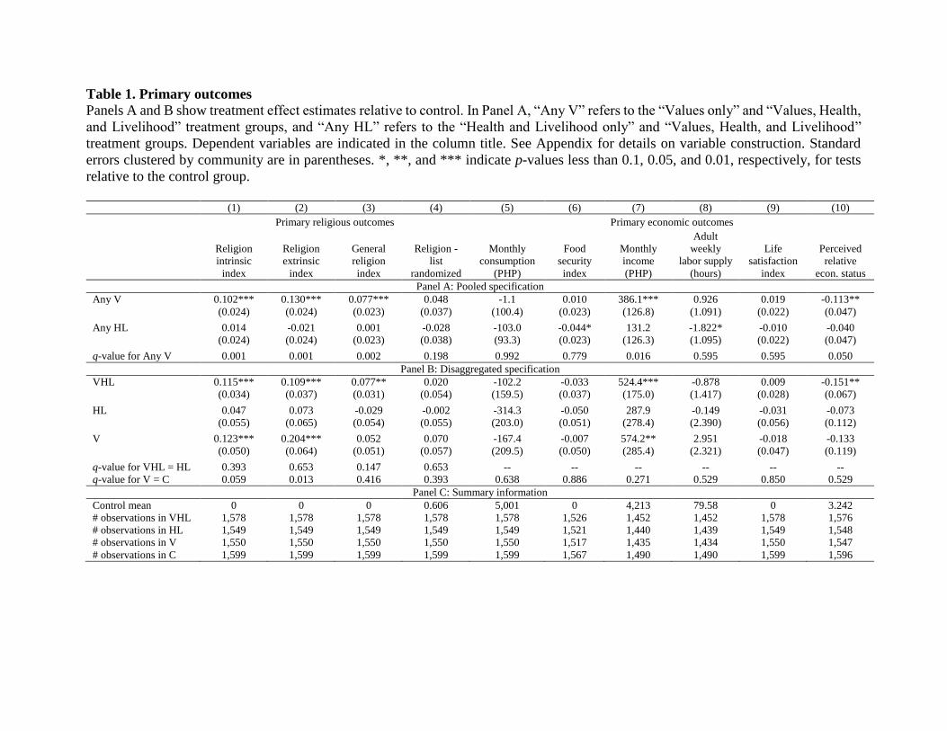
Table 1. Primary outcomes
Panels A and B show treatment effect estimates relative to control. In Panel A, “Any V” refers to the “Values only” and “Values, Health,
and Livelihood” treatment groups, and “Any HL” refers to the “Health and Livelihood only” and “Values, Health, and Livelihood”
treatment groups. Dependent variables are indicated in the column title. See Appendix for details on variable construction. Standard
errors clustered by community are in parentheses. *, **, and *** indicate p-values less than 0.1, 0.05, and 0.01, respectively, for tests
relative to the control group.
(1) (2) (3) (4) (5) (6) (7) (8) (9) (10)
Primary religious outcomes Primary economic outcomes
Religion
intrinsic
index
Religion
extrinsic
index
General
religion
index
Religion -
list
randomized
Monthly
consumption
(PHP)
Food
security
index
Monthly
income
(PHP)
Adult
weekly
labor supply
(hours)
Life
satisfaction
index
Perceived
relative
econ. status
Panel A: Pooled specification
Any V 0.102*** 0.130*** 0.077*** 0.048 -1.1 0.010 386.1*** 0.926 0.019 -0.113**
(0.024) (0.024) (0.023) (0.037) (100.4) (0.023) (126.8) (1.091) (0.022) (0.047)
Any HL 0.014 -0.021 0.001 -0.028 -103.0 -0.044* 131.2 -1.822* -0.010 -0.040
(0.024) (0.024) (0.023) (0.038) (93.3) (0.023) (126.3) (1.095) (0.022) (0.047)
q-value for Any V 0.001 0.001 0.002 0.198 0.992 0.779 0.016 0.595 0.595 0.050
Panel B: Disaggregated specification
VHL 0.115*** 0.109*** 0.077** 0.020 -102.2 -0.033 524.4*** -0.878 0.009 -0.151**
(0.034) (0.037) (0.031) (0.054) (159.5) (0.037) (175.0) (1.417) (0.028) (0.067)
HL 0.047 0.073 -0.029 -0.002 -314.3 -0.050 287.9 -0.149 -0.031 -0.073
(0.055) (0.065) (0.054) (0.055) (203.0) (0.051) (278.4) (2.390) (0.056) (0.112)
V 0.123*** 0.204*** 0.052 0.070 -167.4 -0.007 574.2** 2.951 -0.018 -0.133
(0.050) (0.064) (0.051) (0.057) (209.5) (0.050) (285.4) (2.321) (0.047) (0.119)
q-value for VHL = HL 0.393 0.653 0.147 0.653 -- -- -- -- -- --
q-value for V = C 0.059 0.013 0.416 0.393 0.638 0.886 0.271 0.529 0.850 0.529
Panel C: Summary information
Control mean 0 0 0 0.606 5,001 0 4,213 79.58 0 3.242
# observations in VHL 1,578 1,578 1,578 1,578 1,578 1,526 1,452 1,452 1,578 1,576
# observations in HL 1,549 1,549 1,549 1,549 1,549 1,521 1,440 1,439 1,549 1,548
# observations in V 1,550 1,550 1,550 1,550 1,550 1,517 1,435 1,434 1,550 1,547
# observations in C 1,599 1,599 1,599 1,599 1,599 1,567 1,490 1,490 1,599 1,596

Table 2. Mechanisms
Panels A and B show treatment effect estimates relative to control. In Panel A, “Any V” refers to the “Values
only” and “Values, Health, and Livelihood” treatment groups, and “Any HL” refers to the “Health and Livelihood only” and “Values,
Health, and Livelihood” treatment groups. Dependent variables are indicated in the column title. Indexes have been coded so that more
positive numbers are better. See Appendix for details on variable construction. Standard errors clustered by community are in
parentheses. *, **, and *** indicate p-values less than 0.1, 0.05, and 0.01, respectively, for tests relative to the control group.
(1) (2) (3) (4) (5) (6) (7) (8) (9) (10) (11)
Social capital Locus of control Optimism
Trust
index
Social
safety net
index
Community
activities
index
Perceived
stress scale
index
Powerful
others
index
Locus of
control
index
Life
orientation
index
Expectations
index
Optimism
index
Grit
index
Self-
control
index
Panel A: Pooled specification
Any V 0.004 0.026 0.005 -0.011 0.093*** -0.035* -0.050* -0.037 0.053** 0.041* -0.034*
(0.022) (0.024) (0.025) (0.020) (0.027) (0.020) (0.027) (0.025) (0.024) (0.022) (0.021)
Any HL -0.023 -0.027 0.041 -0.018 0.044 -0.000 0.016 -0.016 -0.024 0.017 0.006
(0.022) (0.024) (0.025) (0.021) (0.027) (0.020) (0.027) (0.025) (0.024) (0.022) (0.020)
p-value for Any V 0.865 0.282 0.851 0.596 0.001 0.075 0.065 0.133 0.029 0.065 0.095
Panel B: Disaggregated specification
VHL -0.019 0.000 0.045 -0.026 0.135*** -0.035 -0.034 -0.055* 0.030 0.056* -0.027
(0.032) (0.032) (0.034) (0.026) (0.038) (0.029) (0.037) (0.032) (0.032) (0.029) (0.025)
HL -0.023 -0.076 0.019 -0.009 0.031 -0.064 -0.046 -0.014 -0.007 0.030 0.039
(0.043) (0.048) (0.058) (0.044) (0.060) (0.057) (0.068) (0.056) (0.061) (0.058) (0.047)
V -0.018 -0.023 -0.011 -0.007 0.073 -0.085* -0.103 -0.054 0.069 0.041 -0.001
(0.046) (0.048) (0.059) (0.043) (0.059) (0.050) (0.069) (0.057) (0.066) (0.058) (0.050)
p-value for VHL = HL 0.927 0.140 0.655 0.684 0.085 0.605 0.862 0.468 0.541 0.671 0.155
p-value for V = C 0.704 0.631 0.857 0.876 0.222 0.090 0.132 0.344 0.298 0.484 0.980
Panel C: Summary information
Control mean 0 0 0 0 0 0 0 0 0 0 0
# observations in VHL 1,578 1,578 1,561 1,577 1,578 1,578 1,578 1,542 1,578 1,578 1,578
# observations in HL 1,549 1,549 1,542 1,549 1,549 1,549 1,549 1,508 1,549 1,549 1,549
# observations in V 1,550 1,550 1,534 1,549 1,550 1,550 1,550 1,518 1,550 1,550 1,550
# observations in C 1,599 1,599 1,592 1,599 1,599 1,599 1,599 1,567 1,599 1,599 1,599

Table 3. Secondary outcomes
Panels A and B show treatment effect estimates relative to control. In Panel A, “Any V” refers to the “Values
only” and “Values, Health, and Livelihood” treatment groups, and “Any HL” refers to the “Health and Livelihood only” and “Values,
Health, and Livelihood” treatment groups. Dependent variables are indicated in the column title. Indexes have been coded so that more
positive numbers are better. See Appendix for details on variable construction. Standard errors clustered by community are in
parentheses. *, **, and *** indicate p-values less than 0.1, 0.05, and 0.01, respectively, for tests relative to the control group.
(1) (2) (3) (4) (5) (6) (7) (8) (9) (10) (11) (12)
Salvation
by grace
belief index
Assets
index
Financial
inclusion
index
Health
index
Hygiene
index,
non-list
random.
Hygiene,
list
random.
House
index
Migration
and
remittance
index
No
discord
index
No
domestic
violence,
list rand.
Child
labor
supply
(hours)
# children
enrolled
in school
Panel A: Pooled specification
Any V -0.036* -0.027 0.020 0.000 0.092*** 0.043 0.030 0.027 -0.034 -0.072 0.244 -0.018
(0.020) (0.021) (0.024) (0.020) (0.024) (0.033) (0.025) (0.019) (0.024) (0.040) (0.215) (0.020)
Any HL -0.005 -0.025 0.157*** 0.015 0.030 0.066 0.007 -0.015 -0.029 -0.048 0.013 -0.018
(0.020) (0.021) (0.025) (0.020) (0.024) (0.033) (0.025) (0.019) (0.024) (0.040) (0.220) (0.020)
p-value for Any V 0.079 0.211 0.396 0.985 0.000 0.191 0.239 0.153 0.164 0.078 0.256 0.376
Panel B: Disaggregated specification
VHL -0.040 -0.050 0.179*** 0.015 0.121*** 0.108** 0.036 0.012 -0.063* -0.118** 0.264 -0.035
(0.026) (0.031) (0.038) (0.028) (0.034) (0.049) (0.036) (0.031) (0.036) (0.055) (0.318) (0.027)
HL -0.021 0.014 0.124** -0.027 0.136* 0.121*** 0.045 -0.083** -0.036 -0.081 -0.074 -0.019
(0.045) (0.057) (0.048) (0.042) (0.070) (0.043) (0.059) (0.038) (0.052) (0.058) (0.376) (0.043)
V -0.061 0.008 -0.010 -0.044 0.208*** 0.105** 0.068 -0.039 -0.049 -0.120** 0.116 -0.019
(0.041) (0.060) (0.044) (0.041) (0.067) (0.045) (0.060) (0.039) (0.049) (0.061) (0.406) (0.042)
p-value for VHL = HL 0.696 0.265 0.297 0.334 0.836 0.779 0.879 0.017 0.617 0.509 0.404 0.688
p-value for V = C 0.143 0.899 0.811 0.285 0.002 0.020 0.258 0.317 0.326 0.050 0.775 0.657
Panel C: Summary information
Control mean 0 0 0 0 0 0.606 0 0 0 0.903 1.555 1.896
# observations in VHL 1,578 1,578 1,578 1,578 1578 1578 1,578 1,578 1,267 1,579 1,452 1,366
# observations in HL 1,549 1,549 1,549 1,549 1549 1549 1,549 1,549 1,297 1,550 1,439 1,341
# observations in V 1,550 1,550 1,550 1,550 1550 1550 1,550 1,550 1,263 1,551 1,434 1,365
# observations in C 1,599 1,599 1,599 1,599 1599 1599 1,599 1,599 1,331 1,600 1,490 1,410

Appendix
Appendix Table 1 shows the questions that constitute our outcome variables. Unless indicated
otherwise in the table, the variable listed in the first column is created by summing its components
listed in the second column. Some components are made up of sub-components, which are shown
to the right of the components. For variables whose name includes the word “index,” if the index
is found in previous academic literature, we use the construction method from that literature, which
in our cases always involves simply summing the components (which are sometimes reverse-
coded, as indicated in the last column). If there is no pre-existing index, we use the index
construction methodology of Kling, Liebman, and Katz (2007). We first sign all variables such
that higher is telling a consistent story for each component of the index. Then we standardize each
component by subtracting its control group mean and dividing by its control group standard
deviation. We compute the sum of the standardized components1 and standardize the sum once
again by the control group sum’s standard deviation.
After data collection, we discovered an issue with our measure of intrinsic religious
orientation. The indexes for intrinsic and extrinsic religious orientation were measured using one
14 question block, with eight questions constituting the intrinsic index and six constituting the
extrinsic index. For each question, respondents were asked to state on a Likert scale a level of
agreement with a statement. In 11 out of the 14 questions, stronger agreement corresponds to
stronger religiosity. In the remaining three—all of which are part of the intrinsic index—weaker
agreement corresponds to stronger religiosity. We believe that respondents did not perceive the
subtle changes in the direction of the questions, causing them to use stronger agreement to express
stronger religiosity even for the reversed questions.2 Thirty-three percent of respondents answered
“agree” or “strongly agree” to all 14 questions, regardless of whether the question was reversed,
whereas only 0.02% of respondents answered “agree” or “strongly” to all non-reversed questions
and “disagree” or “strongly disagree” to all reversed questions. (No respondents answered
1 For observations without information on one or more components of the index, we impute the missing component
standardized values as the mean of the non-missing components’ standardized values for that individual/household. 2 The finding that many subjects indiscriminately agree with statements to express a general support for religion goes
back to the earliest research on intrinsic and extrinsic religious orientation. Allport and Ross (1967) write, “In
responding to the religious items these individuals seem to take a superficial or ‘hit and run’ approach. Their mental
set seems to be ‘all religion is good.’ ‘My religious beliefs are what really lie behind my whole life’—Yes! ‘Although
I believe in my religion, I feel there are many more important things in my life’—Yes!” They classify such types as
the “indiscriminately pro-religious” and find that they are likely to be less educated. This correlation would be
consistent with the high prevalence of such types in our sample of the ultra-poor.

“disagree” or “strongly disagree” to all questions.) Agreement levels are positively correlated
across all seven intrinsic orientation statements, regardless of whether greater agreement
corresponds to greater religiosity or not. We conclude that our intrinsic religious orientation index
should only include the five non-reversed questions, and this five-question intrinsic index is what
we report in Table 1.
If we instead use the eight-question intrinsic measure, as stated in our pre-analysis plan, the
point estimate of the “Any V” treatment effect on intrinsic religious orientation in the pooled
regression specification is 0.04 standard deviations, and its q-value rises to 0.084. In the
disaggregated regression specification, the point estimate of the V versus control effect on intrinsic
religious orientation is 0.01 standard deviations (q = 0.899), and the point estimate of the VHL
versus HL effect on intrinsic religious orientation is 0.074 standard deviations (q = 0.330). The q-
values on the other religious outcomes are qualitatively similar regardless of whether we use the
eight-question or five-question intrinsic measure. Therefore, even though the estimates of the V
curriculum’s effect on intrinsic religious orientation weaken when we use the eight-question
measure, we still find robust first-stage effects on other measures of religiosity.
Online Appendix Tables 5-33 show the treatment effect estimates on each component of the
outcome variables. We also include Online Appendix Table 34, which shows treatment effects on
consumption of “temptation goods” (cigarettes and alcoholic beverages). The categories into
which labor supply is decomposed in Online Appendix Tables 12 and 33 do not correspond exactly
to the categories we asked respondents about. When we looked at the data, we realized that
responses in the labor category of “other” could be manually reclassified into fishing, self-
employment, and other employment with unclear formality. We have also consolidated in the table
the categories of formal employment and operation of a business that is not the household’s, fishing
and livestock tending, and housework in an outside household and daily labor.

Appendix Table 1. Outcome Variable Construction
Variable Components Sub-components (if any) Details Possible answers
Panel A: Primary religious outcomes
Religion
intrinsic index
I enjoy thinking about my religion From Gorsuch and McPherson (1989).
Index formed by adding together
responses without first normalizing.
1 Strongly disagree - 5 Strongly agree
It is important to me to spend time in private thought
and prayer
1 Strongly disagree - 5 Strongly agree
I have often had a strong sense of God's presence 1 Strongly disagree - 5 Strongly agree
I try hard to live all my life according to my
religious beliefs
1 Strongly disagree - 5 Strongly agree
My whole approach to life is based on religion 1 Strongly disagree - 5 Strongly agree
Although I am religious, I don't let it affect my daily
life
This question not used in our main
analysis
1 Strongly agree - 5 Strongly disagree
It doesn't much matter what I believe so long as I am
good
This question not used in our main
analysis
1 Strongly agree - 5 Strongly disagree
Although I believe in my religion, many other things
are more important in life
This question not used in our main
analysis
1 Strongly agree - 5 Strongly disagree
Religion
extrinsic index
I go to religious services because it helps me to
make friends
From Gorsuch and McPherson (1989).
Index formed by adding together
responses without first normalizing.
1 Strongly disagree - 5 Strongly agree
I pray mainly to gain relief and protection 1 Strongly disagree - 5 Strongly agree
What religion offers me most is comfort in times of
trouble and sorrow
1 Strongly disagree - 5 Strongly agree
Prayer is for peace and happiness 1 Strongly disagree - 5 Strongly agree
I go to religious services mostly to spend time with
my friends
I go to religious services mainly because I enjoy
seeing people there
1 Strongly disagree - 5 Strongly agree
1 Strongly disagree - 5 Strongly agree
General religion
index
To what extent do you consider yourself a religious
person?
From the Brief Multidimensional
Measure of Religiousness/Spirituality
(Fetzer Institute 1999)
1 Not religious at all - 4 Very religious
In the last month, have you tried to convince anyone
else to change the way they think about God?
From ICM survey No = 0, Yes = 1
How many people [have you tried to convince]? Adapted from ICM survey Integer ≥ 0

Variable Components Sub-components (if any) Details Possible answers
Panel A: Primary religious outcomes
How often do you go to religious services? Daily = 365, More than once a week =
104, Once a week = 52, Once or twice
a month = 18, Every month or so = 9,
Once or twice a year = 1.5, Never = 0.
In how many of the past 7 days did you pray
privately in places other than at a place of worship?
Integer 0 – 7
How satisfied are you with your spiritual life right
now?
From ICM survey 1 Not at all satisfied - 5 Very satisfied
The Bible is accurate in all that it teaches From ICM survey. These 3 responses are
added together before standardizing, and
then given triple weight when averaging
the components to construct the general
religion index. Asked only of Christians.
1 Strongly disagree - 5 Strongly agree
I believe the Bible has decisive authority over what I
say and do
1 Strongly disagree - 5 Strongly agree
I believe the Christian God—Father, Son, and Holy
Spirit—is the only true God
1 Strongly disagree - 5 Strongly agree
Religion – list
randomized
I have made a personal commitment to Jesus Christ
that is still important to me today
Adapted from ICM survey. Both
questions elicited using list
randomization. Outcome variable is
average of two responses.
False = 0, True = 1
I have read or listened to the Bible in the past week False = 0, True = 1
Panel B: Primary non-religious outcomes
Monthly
consumption
Food consumption in the last week Total amount spent in the last week on
viand, rice/corn/beans/etc.,
bananas/cassava/potatoes/yams/starches/
etc., fruits/vegetables, milk/eggs, non-
alcoholic beverages. Multiplied by 30/7.
Amount in PHP (1 USD 45 PHP in
2015)
Non-food consumption in the last week Total amount spent in the last week on
alcoholic beverages, cigarettes, phone
credit, transportation, clothing/shoes,
soaps/cosmetics, gifts. Multiplied by
30/7.
Amount in PHP (1 USD 45 PHP in
2015)
Average weekly celebration spending in last six
months
Total amount spent on weddings,
funerals, festivals, anniversaries, and
birthdays in the last six months divided
by 6
Amount in PHP (1 USD 45 PHP in
2015)

Variable Components Sub-components (if any) Details Possible answers
Panel B: Primary non-religious outcomes
Food security
index
No household member has gone to bed hungry in
last six months
Constructed from question, “In the last 6
months, did you or any other person in
this household ever go to bed hungry
because there were not enough resources
for food?”
No = 1; Yes = 0; Yes, but during lean
season only = 0
[Lean season in the Philippines is
usually July and August]
No household member has gone to bed hungry in
last six months outside of lean season
Constructed from question, “In the last 6
months, did you or any other person in
this household ever go to bed hungry
because there were not enough resources
for food?”
No = 1; Yes = 0; Yes, but during lean
season only = 1
[Lean season in the Philippines is
usually July and August]
Number of days where no household member has
gone to bed hungry in past seven days
Constructed as 7 minus the number of
days a member of the household has gone
to bed hungry in past seven days
Integer 0 – 7
Monthly income Total household payments received for agricultural
labor on behalf of non-household member
Payments in the last 30 days Amount in PHP (1 USD 45 PHP in
2015)
Total household payments received for formal
employment
Payments in the last 30 days Amount in PHP (1 USD 45 PHP in
2015)
Total household payments received for housework
Payments in the last 30 days Amount in PHP (1 USD 45 PHP in
2015)
Total household payments received for tending
animals in an outside household
Payments in the last 30 days Amount in PHP (1 USD 45 PHP in
2015)
Total household payments received for operating
business that is not the household’s
Payments in the last 30 days Amount in PHP (1 USD 45 PHP in
2015)
Total household payments for daily labor
Payments in the last 30 days Amount in PHP (1 USD 45 PHP in
2015)
Total household payments received for other work
outside the household
Payments in the last 30 days Amount in PHP (1 USD 45 PHP in
2015)
Total profit from household businesses In most recent month with normal sales Amount in PHP (1 USD 45 PHP in
2015)

Variable Components Sub-components (if any) Details Possible answers
Panel B: Primary non-religious outcomes
Adult weekly
labor supply
Total hours spent in outside agricultural labor for
non-household member
During past seven days, only household
members age ≥ 17
Integer
Total hours spent in formal employment During past seven days, only household
members age ≥ 17
Integer
Total hours spent doing housework in an outside
household
During past seven days, only household
members age ≥ 17
Integer
Total hours spent tending animals in an outside
household during past seven days
During past seven days, only household
members age ≥ 17
Integer
Total hours spent operating business that is not the
household’s
During past seven days, only household
members age ≥ 17
Integer
Total hours spent on daily labor During past seven days, only household
members age ≥ 17
Integer
Total hours spent on other work outside the
household
During past seven days, only household
members age ≥ 17
Integer
Life satisfaction
index
Kessler K6 nonspecific
distress scale
About how often during
the past 30 days did you
feel nervous?
From Kessler et al. (2002). Index formed
by adding together responses without
first normalizing.
1 All of the time - 5 none of the time
About how often during
the past 30 days did you
feel hopeless?
1 All of the time - 5 none of the time
About how often during
the past 30 days did you
feel restless or fidgety?
1 All of the time - 5 none of the time
About how often during
the past 30 days did you
feel so depressed that
nothing could you cheer
you up?
1 All of the time - 5 none of the time
About how often during
the past 30 days did you
feel that everything was
difficult?
1 All of the time - 5 none of the time

Variable Components Sub-components (if any) Details Possible answers
Panel B: Primary non-religious outcomes
About how often during
the past 30 days did you
feel worthless?
1 All of the time - 5 none of the time
Sum of 4 Gallup World
Poll questions
Did you experience
enjoyment during a lot
of the day yesterday?
No = 0, Yes = 1
Did you experience
happiness during a lot of
the day yesterday?
No = 0, Yes = 1
Did you experience
worry during a lot of the
day yesterday?
No = 1, Yes = 0
Did you experience
sadness during a lot of
the day yesterday?
No = 1, Yes = 0
Did you smile or laugh a lot yesterday? From Gallup World Poll No = 0, Yes = 1
How would you describe your satisfaction with life? Elicited using Cantril’s ladder 1 Very dissatisfied - 10 Very satisfied
Taking all things together, would you say you are… From World Values Survey 1 Not at all happy - 4 Very happy
Perceived
relative
economic status
Where would you place your household on the
ladder in terms of economic status?
Elicited using Cantril’s ladder 1 Poorest individuals of your
community - 10 Best-off members of
your community
Panel C: Mechanisms
Trust index In general, would you say that most people can be
trusted or that most people cannot be trusted?
Most people can’t be trusted = 0, Most
people can be trusted = 1
Do you think most people would try to take
advantage of you if they got a chance, or would they
try to be fair?
From World Values Survey Try to take advantage of you = 0, Try
to be fair = 1
Would you say that most of the time people try to be
helpful, or that they are mostly just looking out for
themselves?
From General Social Survey Looking out for themselves = 0, Try to
be helpful = 1

Variable Components Sub-components (if any) Details Possible answers
Panel C: Mechanisms
Social safety net
index
In the case where someone in your household did
not have 40 PHP available for an urgent need, how
likely is it that you could access this 40 PHP from a
source outside your household?
1 Very unlikely - 5 Very likely
In the case where someone in your household did
not have 1000 PHP available for an urgent need,
how likely is it that you could access this 1000 PHP
from a source outside your household?
1 Very unlikely - 5 Very likely
Do you discuss personal issues with anyone outside
your close family?
No = 0, Yes = 1
How often do you usually speak to this person? Daily = 365, A few times a week =
104, Weekly = 52, A few times a
month = 24, Monthly = 12, Every
month or so = 9, A few times a year =
6, Yearly = 1. If there is no such
person, coded as 0.
Did anyone from the household receive any meals
from another household in your local community? No = 0, Yes = 1
How many meals [were received]? Top-coded at 99th percentile Integer
Did this household give any meals to anybody from
another household in your local community?
No = 0, Yes = 1
How many meals [were given]? Top-coded at 99th percentile Integer
Community
activities index
Did you attend any village leaders meetings in the
last 6 months?
No = 0, Yes = 1
In the past 6 months, have you participated in any
community activities? No = 0, Yes = 1
How frequently did you participate in community
activities?
Daily = 365, A few times a week =
104, Weekly = 52, A few times a
month = 24, Monthly = 12, Every
month or so = 9, A few times a year =
6, Yearly = 1. If the respondent did
not participate, coded as 0.

Variable Components Sub-components (if any) Details Possible answers
Panel C: Mechanisms
Perceived stress
scale index
How often have you felt that you were unable to
control the important things in your life?
From Cohen et al. (1983). Index formed
by adding together responses without
first normalizing.
1 Very Often - 5 Never
How often have you felt confident about your ability
to handle your personal problems?
1 Never - 5 Very Often
How often have you felt that things were going your
way?
1 Never - 5 Very Often
How often have you felt difficulties were piling up
so high that you could not overcome them?
1 Very Often - 5 Never
Powerful others
index
I feel like what happens in my life is mostly
determined by God
From Levenson (1981) Powerful Others
scale, modified to apply to God’s control
of one’s life. Index formed by adding
together responses without first
normalizing.
1 Strongly disagree - 5 Strongly agree
Although I might have good ability, I will not be
successful without appealing to God
1 Strongly disagree - 5 Strongly agree
My life is chiefly controlled by God 1 Strongly disagree - 5 Strongly agree
Getting what I want requires pleasing God 1 Strongly disagree - 5 Strongly agree
Whether or not I have an accident and hurt myself
physically depends mostly on God
1 Strongly disagree - 5 Strongly agree
In order to have my plans work, I make sure that
they fit with God’s plan for me
1 Strongly disagree - 5 Strongly agree
Locus of control
index
Internality subscale Whether or not I am
successful depends
mostly on my ability
From Levenson (1981). Index formed by
adding together responses without first
normalizing.
1 Strongly disagree - 5 Strongly agree
Whether or not I have an
accident and hurt myself
depends mostly on how
careful I am on a daily
basis
1 Strongly disagree - 5 Strongly agree
When I make plans, I
am almost certain to
make them work
1 Strongly disagree - 5 Strongly agree

Variable Components Sub-components (if any) Details Possible answers
Panel C: Mechanisms
How many friends I
have depends on how
nice a person I am
1 Strongly disagree - 5 Strongly agree
I can pretty much
determine what will
happen in my life
1 Strongly disagree - 5 Strongly agree
I am usually able to
protect my personal
interests
1 Strongly disagree - 5 Strongly agree
When I get what I want
it’s usually because I
worked hard for it
1 Strongly disagree - 5 Strongly agree
My life is determined by
my own actions
1 Strongly disagree - 5 Strongly agree
Chance subscale To a great extent my life
is controlled by
accidental happenings
From Levenson (1981). Index formed by
adding together responses without first
normalizing.
1 Strongly agree - 5 Strongly disagree
Often there is no chance
of protecting my
personal interests from
bad luck happening
1 Strongly agree - 5 Strongly disagree
When I get what I want,
it is usually because I
am lucky
1 Strongly agree - 5 Strongly disagree
I have often found that
what is going to happen
will happen
1 Strongly agree - 5 Strongly disagree
Whether or not I get into
an accident and hurt
myself physically is
mostly a matter of luck
1 Strongly agree - 5 Strongly disagree
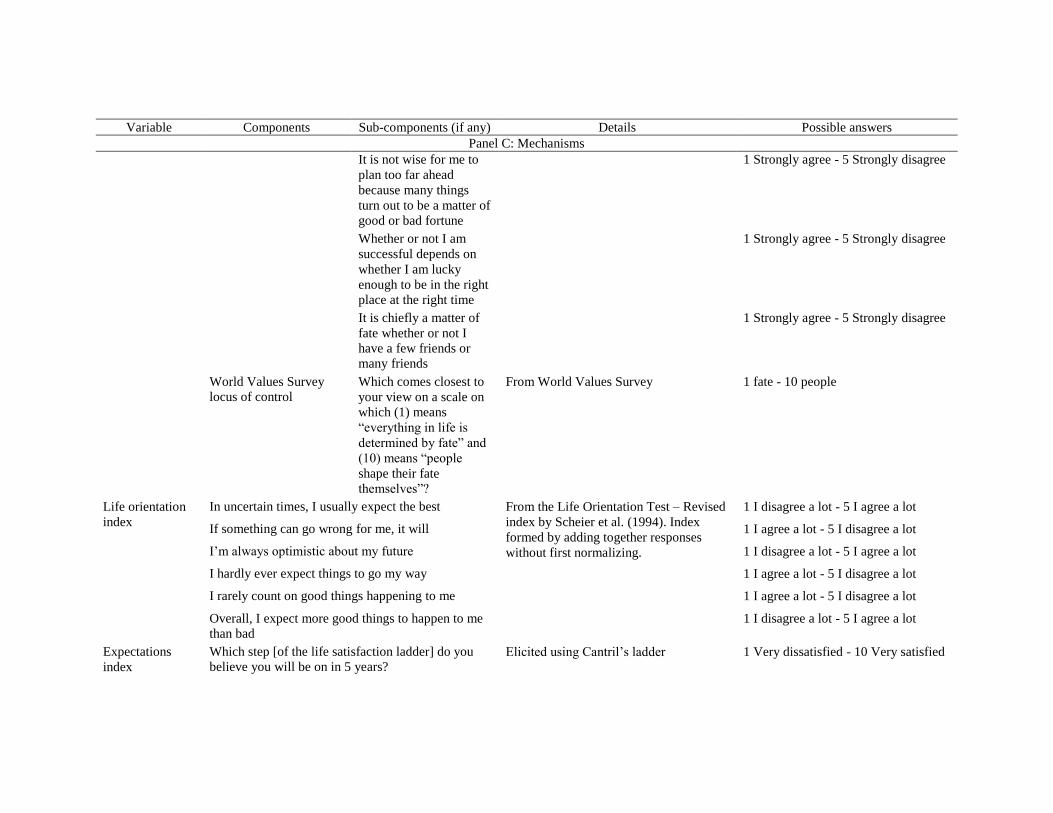
Variable Components Sub-components (if any) Details Possible answers
Panel C: Mechanisms
It is not wise for me to
plan too far ahead
because many things
turn out to be a matter of
good or bad fortune
1 Strongly agree - 5 Strongly disagree
Whether or not I am
successful depends on
whether I am lucky
enough to be in the right
place at the right time
1 Strongly agree - 5 Strongly disagree
It is chiefly a matter of
fate whether or not I
have a few friends or
many friends
1 Strongly agree - 5 Strongly disagree
World Values Survey
locus of control
Which comes closest to
your view on a scale on
which (1) means
“everything in life is
determined by fate” and
(10) means “people
shape their fate
themselves”?
From World Values Survey 1 fate - 10 people
Life orientation
index
In uncertain times, I usually expect the best From the Life Orientation Test – Revised
index by Scheier et al. (1994). Index
formed by adding together responses
without first normalizing.
1 I disagree a lot - 5 I agree a lot
If something can go wrong for me, it will 1 I agree a lot - 5 I disagree a lot
I’m always optimistic about my future 1 I disagree a lot - 5 I agree a lot
I hardly ever expect things to go my way 1 I agree a lot - 5 I disagree a lot
I rarely count on good things happening to me 1 I agree a lot - 5 I disagree a lot
Overall, I expect more good things to happen to me
than bad
1 I disagree a lot - 5 I agree a lot
Expectations
index
Which step [of the life satisfaction ladder] do you
believe you will be on in 5 years? Elicited using Cantril’s ladder 1 Very dissatisfied - 10 Very satisfied

Variable Components Sub-components (if any) Details Possible answers
Panel C: Mechanisms
Where do you think you will be on this [relative
economic status] ladder 5 years from now?
Elicited using Cantril’s ladder 1 Poorest individuals - 10 Best-off
members
Optimism index How optimistic are you in general, on a scale of 1 to
7?
From Scale Optimism-Pessimism-2 by
Kemper et al. (2015). Pessimism scale
shown to respondents had 1 be “not at all
pessimistic” and 7 be “very pessimistic”
1 Not at all optimistic - 7 Very
optimistic
How pessimistic are you in general, on a scale of 1
to 7?
1 Very pessimistic - 7 Not at all
pessimistic
Grit index New ideas and projects sometimes distract me from
previous ones
From the Short Grit Scale (Duckworth
and Quinn 2009). Index formed by
adding together responses without first
normalizing.
1 Very much like me - 5 Not like me
at all
Setbacks don’t discourage me 1 Not like me at all - 5 Very much like
me
I have been obsessed with a certain idea or project
for a short time but later lost interest
1 Very much like me - 5 Not like me
at all
I am a very hard worker 1 Not like me at all - 5 Very much like
me
I often set a goal but later choose to pursue a
different one
1 Very much like me - 5 Not like me
at all
I have difficulty maintaining my focus on projects
that take more than a few months
1 Very much like me - 5 Not like me
at all
I finish whatever I begin 1 Not like me at all - 5 Very much like
me
I am diligent
1 Not like me at all - 5 Very much like
me
Self-control
index
I have a hard time breaking bad habits Subset of the Brief Self-Control Scale by
Tangney, Baumeister, and Boone (2004).
Index formed by adding together
responses without first normalizing.
1 Very much like me - 5 Not like me
at all
I get distracted easily 1 Very much like me - 5 Not like me
at all
I say inappropriate things 1 Very much like me - 5 Not like me
at all
I refuse things that are bad for me, even if they are
fun 1 Not like me at all - 5 Very much like
me

Variable Components Sub-components (if any) Details Possible answers
Panel C: Mechanisms
I’m good at resisting temptation 1 Not like me at all - 5 Very much like
me
People would say that I have very strong self-
discipline 1 Not like me at all - 5 Very much like
me
Pleasure and fun sometimes keep me from getting
work done
1 Very much like me - 5 Not like me
at all
I do things that feel good in the moment but regret
later on
1 Very much like me - 5 Not like me
at all
Sometimes I can’t stop myself from doing
something, even if I know it’s wrong
1 Very much like me - 5 Not like me
at all
I often act without thinking through all the
alternatives
1 Very much like me - 5 Not like me
at all
Panel D: Secondary outcomes
Salvation by
grace belief
index
If I am good enough, God will cleanse me of my
sins
Question asked only of Christians 1 Strongly agree - 5 Strongly disagree
I follow God’s laws so that I can go to heaven Question asked only of Christians 1 Strongly agree - 5 Strongly disagree
Which of the following best describes your belief
about what happens after death?
There is no life after death = 0; I will
go to heaven because I tried my best
to be a good person and to live a good
life = 0; I will go to heaven because I
tried to be involved in my religion,
pray, and live the way I think God
wants me to = 0; I will go to hell = 0;
I’m not sure if I will go to heaven or
hell = 0; I will be reincarnated = 0;
My belief is not well-described by any
of these choices = 0; I will go to
heaven because I have accepted Jesus
Christ as my personal savior = 1

Variable Components Sub-components (if any) Details Possible answers
Panel D: Secondary outcomes
Assets index Chance that you, or someone in your household,
would have 40 PHP available for your use in this
circumstance of urgent need?
1 Very unlikely - 5 Very likely
Chance that you, or someone in your household,
would have 1,000 PHP available for your use in this
circumstance of urgent need?
1 Very unlikely - 5 Very likely
Number of productive assets acquired in last 6
months
Number of the following acquired in the
last 6 months: tractors, sewing machines
and farm tools. Top-coded at 99th
percentile.
Integer ≥ 0
Value of the productive assets in the household
acquired in the last 6 months
Sum of the amount paid for the above
categories of assets. Top-coded at 99th
percentile.
Value of assets in PHP (1 USD 45
PHP in 2015)
Number of house assets acquired in last 6 months Number of the following acquired in the
last 6 months: TV,
VTR/VHS/VCD/DVD player,
radio/transistor/stereo, electric fan,
refrigerator/freezer, telephone/mobile
phone, sala set, bicycle or pedicab ,
motorcab or motorcycle, boat, washing
machine, chair/stool, bed or cot, table,
watch or clock, jewelry, gas stove. Top-
coded at 99th percentile.
Integer ≥ 0
Value of the house assets acquired in the last 6
months
Sum of the amount paid for the above
categories of assets. Top-coded at 99th
percentile.
Value of assets in PHP (1 USD 45
PHP in 2015)
Number of productive assets (level) Number of tractors, sewing machines,
and farm tools owned. Top-coded at 99th
percentile.
Integer ≥ 0
Value of productive assets (level) Sum of the amount paid for the above
assets. Top-coded at 99th percentile. Value of assets in PHP (1 USD 45
PHP in 2015)
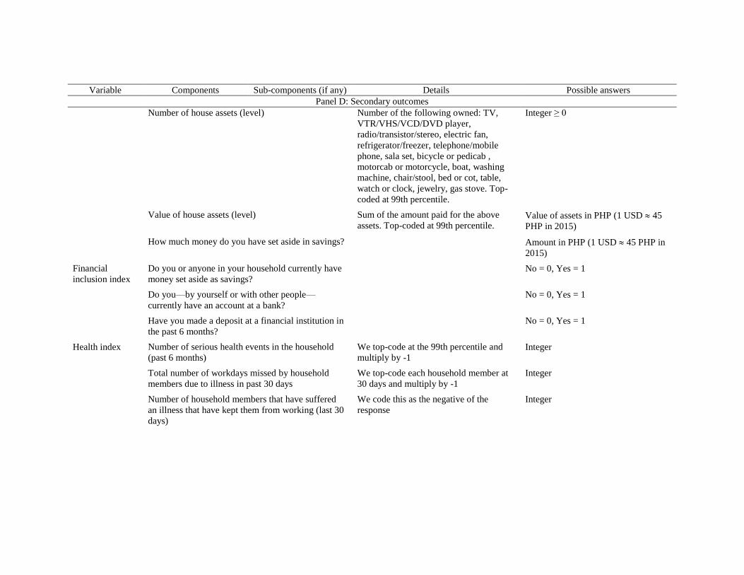
Variable Components Sub-components (if any) Details Possible answers
Panel D: Secondary outcomes
Number of house assets (level) Number of the following owned: TV,
VTR/VHS/VCD/DVD player,
radio/transistor/stereo, electric fan,
refrigerator/freezer, telephone/mobile
phone, sala set, bicycle or pedicab ,
motorcab or motorcycle, boat, washing
machine, chair/stool, bed or cot, table,
watch or clock, jewelry, gas stove. Top-
coded at 99th percentile.
Integer ≥ 0
Value of house assets (level) Sum of the amount paid for the above
assets. Top-coded at 99th percentile. Value of assets in PHP (1 USD 45
PHP in 2015)
How much money do you have set aside in savings? Amount in PHP (1 USD 45 PHP in
2015)
Financial
inclusion index
Do you or anyone in your household currently have
money set aside as savings?
No = 0, Yes = 1
Do you—by yourself or with other people—
currently have an account at a bank?
No = 0, Yes = 1
Have you made a deposit at a financial institution in
the past 6 months?
No = 0, Yes = 1
Health index Number of serious health events in the household
(past 6 months)
We top-code at the 99th percentile and
multiply by -1
Integer
Total number of workdays missed by household
members due to illness in past 30 days
We top-code each household member at
30 days and multiply by -1
Integer
Number of household members that have suffered
an illness that have kept them from working (last 30
days)
We code this as the negative of the
response
Integer

Variable Components Sub-components (if any) Details Possible answers
Panel D: Secondary outcomes
Hygiene index,
non-list
randomized
Own or lease animals that are not kept in a separate
stable
No = 1, Yes = 0
At least one household member practices open
defecation
Coded yes if primary latrine is forest,
bushes, fields, bodies of water, hanging
latrine, uncovered pit latrine, open pit
No = 1, Yes = 0
Hygiene, list-
randomized
I treat my water before drinking it, for example by
using solar disinfection, boiling it, or using a water
filter
Both questions elicited using list
randomization. Outcome variable is
average of two components’ responses
No = 0, Yes = 1
I wash my hands after going to the bathroom No = 0, Yes = 1
House index Are all rooms leak-free? No = 0, Yes = 1
Are at least some rooms leak-free? No = 0, Yes = 1
Are all rooms able to be safely locked? No = 0, Yes = 1
Are at least some rooms able to be safely locked? No = 0, Yes = 1
Primary source of energy for lighting is electricity No = 0, Yes = 1
Primary latrine is inside the house No = 0, Yes = 1
Migration and
remittance index
Number of migrators in the household Number of household members who have
slept outside the house for more than two
consecutive nights for work in the past
six months
Integer
Number of days migrators in the household were
gone in the last six months
Integer
Number of migrators who sent remittances or
brought money home to the household in the last six
months
Integer
Household had at least one migrator who sent
remittances or brought cash home in the last six
months
No = 0, Yes = 1
Amount received in remittances or cash brought
home by household migrators in the last six months
Amount in PHP (1 USD 45 PHP in
2015)

Variable Components Sub-components (if any) Details Possible answers
Panel D: Secondary outcomes
No discord index During the last one month, did you have any major
arguments with your spouse or partner over
spending on major household items or assets?
No = 1, Yes = 0
During the last one month, did you have any major
arguments with your spouse or partner over saving
decisions?
No = 1, Yes = 0
During the last one month, did you have any major
arguments with your spouse or partner over the
behavior and disciplining of children?
No = 1, Yes = 0
During the last one month, did you have any major
arguments with your spouse or partner over
interactions with relatives?
No = 1, Yes = 0
During the last one month, did you have any major
arguments with your spouse or partner over alcohol
consumption?
No = 1, Yes = 0
During the last one month, did you have any major
arguments with your spouse or partner over any
other issues?
No = 1, Yes = 0
No domestic
violence, list
randomized
Someone in my household is experiencing physical
abuse
Question elicited using list
randomization.
No = 1, Yes = 0
Child labor
supply
Total hours spent in outside agricultural labor for
non-household member
During past seven days, only household
members age ≤ 16
Integer
Total hours spent in formal employment During past seven days, only household
members age ≤ 16
Integer
Total hours spent doing housework in an outside
household
During past seven days, only household
members age ≤ 16
Integer
Total hours spent tending animals in an outside
household during past seven days
During past seven days, only household
members age ≤ 16
Integer

Variable Components Sub-components (if any) Details Possible answers
Panel D: Secondary outcomes
Total hours spent operating business that is not the
household’s
During past seven days, only household
members age ≤ 16
Integer
Total hours spent on daily labor During past seven days, only household
members age ≤ 16
Integer
Total hours spent on other work outside the
household
During past seven days, only household
members age ≤ 16
Integer
# children
enrolled in
school
Age ≤ 16 Integer

Online Appendix
Randomizing Religion: The Impact of Protestant Evangelism on Economic
Outcomes
Gharad Bryan, James J. Choi, Dean Karlan
This file includes the following tables:
a. Balance across treatment groups
Online Appendix Table 1: Pre-treatment characteristics (collected in 6-month survey)
b. Main results including communities that switched treatments
Online Appendix Table 2: Primary outcomes (including communities that switched treatment
status)
Online Appendix Table 3: Mechanisms (including communities that switched treatment
status)
Online Appendix Table 4: Secondary outcomes (including communities that switched
treatment status)
c. Results by components
Online Appendix Table 5: Religion intrinsic index
Online Appendix Table 6: Religion extrinsic index
Online Appendix Table 7: General religion index
Online Appendix Table 8: Religion – list randomized
Online Appendix Table 9: Monthly consumption
Online Appendix Table 10: Food security index
Online Appendix Table 11: Monthly income
Online Appendix Table 12: Adult labor supply
Online Appendix Table 13: Life satisfaction index
Online Appendix Table 14: Perceived relative economic wellbeing
Online Appendix Table 15: Trust index
Online Appendix Table 16: Social safety net index
Online Appendix Table 17: Community activities index
Online Appendix Table 18: Perceived stress scale index
Online Appendix Table 19: Powerful Others Subscale
Online Appendix Table 20a: Locus of control index: Internality subscale

Online Appendix Table 20b: Locus of control index: Chance subscale and World Value
Survey question
Online Appendix Table 21: Life orientation index
Online Appendix Table 22: Expectations index and optimism index
Online Appendix Table 23: Grit index
Online Appendix Table 24: Self-control index
Online Appendix Table 25: Salvation by grace belief index
Online Appendix Table 26: Assets index
Online Appendix Table 27: Financial inclusion index
Online Appendix Table 28: Health index
Online Appendix Table 29: Hygiene Indices
Online Appendix Table 30: House index
Online Appendix Table 31: Migration and remittance index
Online Appendix Table 32: No discord index and no domestic violence – list randomized
Online Appendix Table 33: Child labor supply and children enrolled in school
d. Temptation goods
Online Appendix Table 34: Consumption of temptation goods
e. Robustness checks
Online Appendix Table 35: Income robustness checks
f. Religion checks
Online Appendix Table 36: Summary statistics on religious affiliation by treatment group
Online Appendix Table 37: Treatment effects on binary variables for Catholic and Protestant
respondents

Online Appendix Table 1. Pre-treatment characteristics (collected in 6-month survey)
Control V HL VHLC vs. V,
p -value
C vs. HL,
p -value
C vs. VHL,
p -value
V vs. HL,
p -value
V vs. VHL,
p -value
HL vs. VHL,
p -value
p -value from joint test of
equality across arms
Average number of household 5.166 5.263 5.105 5.025 0.328 0.540 0.165 0.125 0.023 0.448 0.132
members (0.068) (0.073) (0.073) (0.075)
2.765 2.808 2.810 2.733 0.440 0.416 0.559 0.966 0.207 0.194 0.497
(0.036) (0.041) (0.041) (0.043)
2.385 2.430 2.287 2.279 0.587 0.265 0.203 0.096 0.062 0.928 0.184
(0.060) (0.057) (0.064) (0.058)
% female respondents 0.832 0.849 0.833 0.834 0.444 0.967 0.923 0.520 0.518 0.963 0.863
(0.016) (0.016) (0.019) (0.017)
% married respondents 0.794 0.741 0.786 0.771 0.018 0.712 0.281 0.052 0.210 0.488 0.102
(0.013) (0.018) (0.015) (0.016)
7.737 7.772 7.727 7.654 0.917 0.976 0.808 0.894 0.724 0.833 0.988
(0.239) (0.225) (0.246) (0.248)
% ICM Base: Koronoadal 0.246 0.232 0.234 0.241 0.849 0.865 0.951 0.984 0.896 0.913 0.997
(0.051) (0.050) (0.050) (0.050)
% ICM Base: General Santos 0.233 0.245 0.241 0.237 0.863 0.912 0.956 0.951 0.906 0.956 0.998
(0.047) (0.050) (0.050) (0.048)
% ICM Base: Bacolod 0.271 0.263 0.270 0.268 0.912 0.990 0.971 0.922 0.941 0.981 1.000
(0.053) (0.052) (0.053) (0.052)
% ICM Base: Dumaguete 0.250 0.260 0.256 0.253 0.890 0.938 0.962 0.952 0.927 0.976 0.999
(0.049) (0.051) (0.051) (0.050)
154.439 156.865 147.488 153.984 0.719 0.304 0.951 0.130 0.678 0.351 0.476
(5.144) (4.360) (4.385) (5.414)
0.836 0.831 0.849 0.825 0.807 0.467 0.606 0.296 0.769 0.193 0.557
(0.015) (0.014) (0.011) (0.015)
Number of observations 1,599 1,550 1,549 1,578
These numbers exclude the five community pairs that did not comply with their treatment assignment. The average number of household members is not exactly equal to the sum of the average number of adults
and the average number of children because of missing ages in the data. Standard errors clustered by community are in parentheses. The following educational categories are coded as corresponding to the
following number of years of education: Pre-school only = 0.5, some grade 12 education without high school graduation = 12, high school graduation = 13, partial vocational education = 14, complete vocational
education = 15, partial college = 16, college graduation = 17.
Average number of children
(age < 17) in the household
Average number of adults
(age ≥ 17) in the household
Average years of education of
respondent
# days between June 1 2015 and
interview end date
% households successfully
interviewed

1 2 3 4 5 6 7 8 9 10
Religion
intrinsic index
Religion
extrinsic index
General
religion index
Religion - list
randomization
Monthly
consumption
(PHP)
Food security
index
Monthly
income
(PHP)
Adult weekly
labor supply
(hours)
Life
satisfaction
index
Perceived
relative econ.
status
Panel A: Pooled specification
Any V 0.098*** 0.129*** 0.069*** 0.053 4.907 0.013 380.3*** 0.814 0.024 -0.105**
(0.023) (0.023) (0.022) (0.036) (98.76) (0.022) (123.9) (1.057) (0.022) (0.046)
[0.001] [0.001] [0.003] [0.145] [0.961] [0.655] [0.014] [0.655] [0.539] [0.070]
Any HL 0.011 -0.023 -0.000 -0.018 -59.151 -0.034 111.9 -1.550 -0.012 -0.033
(0.023) (0.023) (0.022) (0.036) (91.50) (0.022) (123.4) (1.070) (0.022) (0.046)
VHL 0.108*** 0.106*** 0.070** 0.035 -55.32 -0.020 500.8*** -0.773 0.012 -0.136**
(0.033) (0.036) (0.029) (0.052) (154.8) (0.036) (171.5) (1.362) (0.027) (0.065)
HL 0.044 0.089 -0.032 0.001 -297.47 -0.033 220.4 -0.208 -0.027 -0.099
(0.053) (0.063) (0.052) (0.053) (195.2) (0.050) (270.1) (2.327) (0.055) (0.109)
V 0.118** 0.219*** 0.041 0.068 -187.38 0.002 531.0* 2.556 -0.010 -0.155
(0.048) (0.062) (0.049) (0.055) (202.3) (0.049) (277.1) (2.249) (0.046) (0.116)
p-value for VHL = HL test 0.255 0.793 0.056 0.467 0.233 0.786 0.292 0.809 0.484 0.737
q-value for VHL = HL test [0.409] [0.794] [0.151] [0.534] -- -- -- -- -- --
p-value for V = C test 0.0154 0.0005 0.4040 0.2156 0.3549 0.9704 0.0563 0.2565 0.8351 0.1806
q-value for V = C test [0.062] [0.005] [0.534] [0.409] [0.533] [0.971] [0.338] [0.514] [0.971] [0.514]
Panel C: Summary information
Control group mean 0 0 0 0.609 4,995 0 4,241 79.86 0 3.236
# observations in VHL 1,646 1,646 1,646 1,646 1,646 1,594 1,520 1,520 1,646 1,644
# observations in HL 1,596 1,596 1,596 1,596 1,596 1,568 1,487 1,486 1,596 1,595
# observations in V 1,598 1,598 1,598 1,598 1,598 1,556 1,482 1,481 1,598 1,595
# observations in C 1,667 1,667 1,667 1,667 1,667 1,635 1,557 1,557 1,667 1,664
Results in this table include observations from communities that did not follow the original treatment assignment and switched treatment status. Panels A and B show treatment effect estimates
relative to control. In Panel A, “Any V” refers to the “Values only” and “Values, Health, and Livelihood” treatment groups, and “Any HL” refers to the “Health and Livelihood only” and
“Values, Health, and Livelihood” treatment groups. Dependent variables are indicated in the column title. See Appendix for details on variable construction. Standard errors clustered by
community are in parentheses, and q -values are in brackets. The q -values in Panel A are for tests of effects relative to the control group. *, **, and *** indicate p -values less than 0.1, 0.05, and
0.01, respectively, for tests relative to the control group.
Online Appendix Table 2. Primary outcomes (including communities that switched treatment status)
Panel B: Disaggregated specification

11 12 13 14 15 16 17 18 19 20 21
Trust indexSocial safety
net index
Commmunit
y activities
index
Perceived
stress scale
index
Powerful
others index
Locus of
control index
Life
orientation
index
Expectations
index
Optimism
indexGrit index
Self-control
index
Panel A: Pooled specification
Any V 0.006 0.031 0.012 -0.008 0.093*** -0.037* -0.034 -0.032 0.050** 0.056** -0.040**
(0.022) (0.023) (0.025) (0.020) (0.027) (0.019) (0.027) (0.024) (0.024) (0.022) (0.020)
Any HL -0.013 -0.026 0.033 -0.019 0.032 0.000 0.012 -0.026 -0.032 0.015 0.007
(0.022) (0.023) (0.025) (0.020) (0.027) (0.019) (0.027) (0.025) (0.023) (0.022) (0.020)
Panel B: Disaggregated specification
VHL -0.007 0.006 0.045 -0.026 0.125*** -0.036 -0.022 -0.061* 0.018 0.067** -0.031
(0.032) (0.031) (0.034) (0.025) (0.038) (0.028) (0.036) (0.031) (0.032) (0.029) (0.024)
HL -0.010 -0.070 0.020 -0.010 0.028 -0.059 -0.056 -0.027 -0.016 0.033 0.029
(0.043) (0.047) (0.057) (0.043) (0.059) (0.055) (0.066) (0.055) (0.060) (0.057) (0.046)
V -0.014 -0.013 0.005 -0.004 0.080 -0.082* -0.093 -0.054 0.066 0.057 -0.020
(0.045) (0.047) (0.059) (0.042) (0.058) (0.049) (0.068) (0.055) (0.065) (0.058) (0.049)
p-value for VHL = HL test 0.948 0.131 0.672 0.710 0.102 0.675 0.617 0.544 0.567 0.553 0.188
p-value for V = C test 0.754 0.778 0.931 0.930 0.169 0.097 0.173 0.326 0.307 0.332 0.682
Panel C: Summary information
Control group mean 0 0 0 0 0 0 0 0 0 0 0
# observations in VHL 1,646 1,646 1,629 1,645 1,646 1,646 1,646 1,610 1,646 1,646 1,646
# observations in HL 1,596 1,596 1,589 1,596 1,596 1,596 1,596 1,555 1,596 1,596 1,596
# observations in V 1,598 1,598 1,582 1,597 1,598 1,598 1,598 1,565 1,598 1,598 1,598
# observations in C 1,667 1,667 1,660 1,667 1,667 1,667 1,667 1,631 1,667 1,667 1,667
Results in this table include observations from communities that did not follow the original treatment assignment and switched treatment status. Panels A and B show treatment effect estimates
relative to control. In Panel A, “Any V” refers to the “Values only” and “Values, Health, and Livelihood” treatment groups, and “Any HL” refers to the “Health and Livelihood only” and
“Values, Health, and Livelihood” treatment groups. Dependent variables are indicated in the column title. Indexes have been coded so that more positive numbers are better. See Appendix for
details on variable construction. Standard errors clustered by community are in parentheses. *, **, and *** indicate p -values less than 0.1, 0.05, and 0.01, respectively, for tests relative to the
control group.
Online Appendix Table 3. Mechanisms (including communities that switched treatment status)

22 23 24 25 26 27 28 29 30 31 32 33
Salvation
by grace
belief index
Assets
index
Financial
inclusion
index
Health
index
Hygiene
index, non-
list random.
Hygiene,
list random.
House
index
Migration
and
remittance
index
No discord
index
No
domestic
violence,
list rand.
Child labor
supply
(hours)
# children
enrolled in
school
Panel A: Pooled specification
Any V -0.036* -0.021 0.022 -0.000 0.078*** 0.043 0.040 0.026 -0.037 -0.074* 0.334 -0.022
(0.020) (0.021) (0.023) (0.020) (0.024) (0.033) (0.025) (0.019) (0.024) (0.040) (0.209) (0.019)
Any HL -0.006 -0.021 0.143*** 0.021 0.030 0.070** 0.010 -0.007 -0.028 -0.054 -0.021 -0.016
(0.020) (0.021) (0.025) (0.019) (0.024) (0.033) (0.025) (0.019) (0.024) (0.040) (0.215) (0.019)
Panel B: Disaggregated specification
VHL -0.043* -0.041 0.165*** 0.020 0.108*** 0.111** 0.050 0.020 -0.064* -0.127** 0.313 -0.038
(0.025) (0.030) (0.038) (0.027) (0.034) (0.049) (0.036) (0.030) (0.034) (0.054) (0.306) (0.026)
HL -0.025 0.011 0.101** -0.013 0.121* 0.127*** 0.045 -0.062 -0.038 -0.100* -0.076 -0.018
(0.045) (0.055) (0.048) (0.041) (0.070) (0.042) (0.057) (0.040) (0.050) (0.058) (0.370) (0.042)
V -0.065 0.008 -0.016 -0.037 0.182*** 0.108** 0.073 -0.028 -0.054 -0.135** 0.244 -0.025
(0.041) (0.058) (0.044) (0.040) (0.067) (0.044) (0.059) (0.039) (0.048) (0.059) (0.396) (0.041)
p-value for VHL = HL test 0.710 0.340 0.216 0.444 0.849 0.717 0.933 0.048 0.617 0.642 0.328 0.620
p-value for V = C test 0.113 0.898 0.719 0.359 0.007 0.014 0.213 0.475 0.266 0.023 0.539 0.547
Panel C: Summary information
Control group mean 0 0 0 0 0 1 0 0 0 0 1 2
# observations in VHL 1,646 1,646 1,646 1,646 1,646 1,646 1,646 1,646 1,327 1,646 1,520 1,426
# observations in HL 1,596 1,596 1,596 1,596 1,596 1,596 1,596 1,596 1,342 1,596 1,486 1,384
# observations in V 1,598 1,598 1,598 1,598 1,598 1,598 1,598 1,598 1,306 1,598 1,481 1,406
# observations in C 1,667 1,667 1,667 1,667 1,667 1,667 1,667 1,667 1,390 1,667 1,557 1,472
Results in this table include observations from communities that did not follow the original treatment assignment and switched treatment status. Panels A and B show treatment effect
estimates relative to control. In Panel A, “Any V” refers to the “Values only” and “Values, Health, and Livelihood” treatment groups, and “Any HL” refers to the “Health and Livelihood
only” and “Values, Health, and Livelihood” treatment groups. Dependent variables are indicated in the column title. Indexes have been coded so that more positive numbers are better. See
Appendix for details on variable construction. Standard errors clustered by community are in parentheses. *, **, and *** indicate p -values less than 0.1, 0.05, and 0.01, respectively, for
tests relative to the control group.
Online Appendix Table 4. Secondary outcomes (including communities that switched treatment status)

1 2 3 4 5 6 7 8 9
Religion
intrinsic index -
5 questions
I enjoy
thinking
about my
religion
It is important to
me to spend time
in private thought
and prayer
I have often
had a strong
sense of God's
presence
I try hard to
live all my life
according to
my religious
beliefs
My whole
approach to
life is based on
religion
Although I am
religious, I don't
let it affect my
daily life
(not used)
It doesn't much
matter what I
believe so long
as I am good
(not used)
Although I believe
in my religion,
many other things
are more important
in life (not used)
Panel A: Pooled specification
Any V 0.102*** 0.017 0.029* 0.033** 0.077*** 0.133*** 0.062*** 0.029 0.079***
(0.024) (0.014) (0.015) (0.016) (0.022) (0.030) (0.024) (0.022) (0.029)
Any HL 0.014 -0.023* -0.005 0.014 0.043* 0.012 0.008 0.004 0.024
(0.024) (0.014) (0.015) (0.016) (0.023) (0.030) (0.023) (0.022) (0.028)
Panel B: Disaggregated specification
VHL 0.115*** -0.007 0.023 0.047** 0.120*** 0.143*** 0.070** 0.032 0.102**
(0.034) (0.019) (0.021) (0.024) (0.031) (0.042) (0.033) (0.030) (0.046)
HL 0.047 -0.010 0.003 0.032 0.060 0.047 0.077 0.038 0.115*
(0.055) (0.036) (0.030) (0.028) (0.051) (0.074) (0.056) (0.041) (0.064)
V 0.123** 0.028 0.028 0.049* 0.084* 0.162** 0.125** 0.057 0.154**
(0.050) (0.034) (0.030) (0.028) (0.046) (0.071) (0.058) (0.039) (0.064)
p -value for VHL = HL test 0.246 0.932 0.532 0.648 0.254 0.208 0.909 0.889 0.849
p -value for V = C test 0.015 0.417 0.343 0.083 0.070 0.022 0.032 0.147 0.016
Panel C: Summary information
Control group mean 0 4.570 4.710 4.701 4.341 3.766 4.236 4.530 3.868
# observations in VHL 1,578 1,578 1,578 1,578 1,578 1,578 1,578 1,578 1,578
# observations in HL 1,549 1,549 1,549 1,549 1,549 1,549 1,549 1,549 1,549
# observations in V 1,550 1,550 1,550 1,550 1,550 1,550 1,550 1,550 1,550
# observations in C 1,599 1,599 1,599 1,599 1,599 1,599 1,599 1,599 1,599
Online Appendix Table 5. Religion intrinsic index
Panels A and B show treatment effect estimates relative to control. Dependent variables are indicated in the column title. Variables have been coded so that more positive numbers
correspond to greater religiosity. See Appendix for details on variable construction. The variables to the right of the first column have not been standardized. Standard errors clustered by
community are in parentheses. *, **, and *** indicate p -values less than 0.1, 0.05, and 0.01, respectively, for tests relative to the control group.
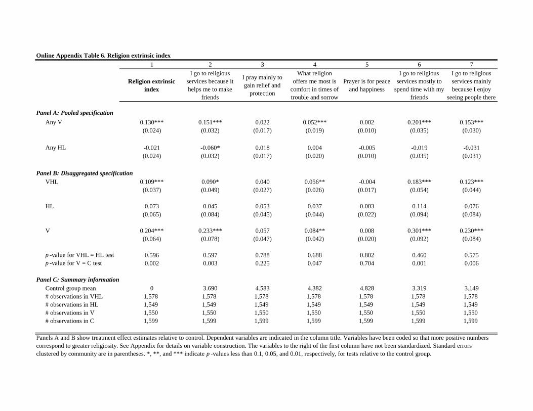
1 2 3 4 5 6 7
Religion extrinsic
index
I go to religious
services because it
helps me to make
friends
I pray mainly to
gain relief and
protection
What religion
offers me most is
comfort in times of
trouble and sorrow
Prayer is for peace
and happiness
I go to religious
services mostly to
spend time with my
friends
I go to religious
services mainly
because I enjoy
seeing people there
Panel A: Pooled specification
Any V 0.130*** 0.151*** 0.022 0.052*** 0.002 0.201*** 0.153***
(0.024) (0.032) (0.017) (0.019) (0.010) (0.035) (0.030)
Any HL -0.021 -0.060* 0.018 0.004 -0.005 -0.019 -0.031
(0.024) (0.032) (0.017) (0.020) (0.010) (0.035) (0.031)
Panel B: Disaggregated specification
VHL 0.109*** 0.090* 0.040 0.056** -0.004 0.183*** 0.123***
(0.037) (0.049) (0.027) (0.026) (0.017) (0.054) (0.044)
HL 0.073 0.045 0.053 0.037 0.003 0.114 0.076
(0.065) (0.084) (0.045) (0.044) (0.022) (0.094) (0.084)
V 0.204*** 0.233*** 0.057 0.084** 0.008 0.301*** 0.230***
(0.064) (0.078) (0.047) (0.042) (0.020) (0.092) (0.084)
p -value for VHL = HL test 0.596 0.597 0.788 0.688 0.802 0.460 0.575
p -value for V = C test 0.002 0.003 0.225 0.047 0.704 0.001 0.006
Panel C: Summary information
Control group mean 0 3.690 4.583 4.382 4.828 3.319 3.149
# observations in VHL 1,578 1,578 1,578 1,578 1,578 1,578 1,578
# observations in HL 1,549 1,549 1,549 1,549 1,549 1,549 1,549
# observations in V 1,550 1,550 1,550 1,550 1,550 1,550 1,550
# observations in C 1,599 1,599 1,599 1,599 1,599 1,599 1,599
Online Appendix Table 6. Religion extrinsic index
Panels A and B show treatment effect estimates relative to control. Dependent variables are indicated in the column title. Variables have been coded so that more positive numbers
correspond to greater religiosity. See Appendix for details on variable construction. The variables to the right of the first column have not been standardized. Standard errors
clustered by community are in parentheses. *, **, and *** indicate p -values less than 0.1, 0.05, and 0.01, respectively, for tests relative to the control group.

1 2 3 4 5 6 7 8
General religion
index
To what extent do
you consider
yourself a religious
person?
In the last month, have you
tried to convince anyone else
to change the way they think
about God?
How many people?
In how many of the past 7
days did you pray privately
in places other than at a
place of worship?
How satisfied are
you with your
spiritual life right
now?
How often do you
go to religious
service? (number of
days in a year)
ICM religion
Panel A: Pooled specification
Any V 0.077*** 0.020 0.012 0.028 0.201*** -0.013 0.937 0.121***
(0.023) (0.017) (0.009) (0.052) (0.066) (0.020) (0.621) (0.039)
Any HL 0.001 -0.004 -0.026*** 0.000 -0.111* 0.011 -1.382** 0.081**
(0.023) (0.016) (0.009) (0.053) (0.064) (0.020) (0.621) (0.040)
Panel B: Disaggregated specification
VHL 0.077** 0.016 -0.014 0.026 0.092 -0.002 -0.438 0.202***
(0.031) (0.023) (0.013) (0.070) (0.087) (0.024) (0.803) (0.050)
HL -0.029 -0.028 -0.042** -0.063 -0.153 0.009 -0.668 0.047
(0.054) (0.035) (0.021) (0.119) (0.162) (0.042) (1.438) (0.087)
V 0.052 -0.009 -0.002 -0.022 0.109 -0.017 1.832 0.100
(0.051) (0.035) (0.020) (0.089) (0.150) (0.046) (1.412) (0.084)
p -value for VHL = HL test 0.055 0.215 0.189 0.475 0.142 0.806 0.870 0.074
p -value for V = C test 0.312 0.790 0.933 0.801 0.469 0.718 0.196 0.232
Panel C: Summary information
Control group mean 0 2.795 0.301 0.887 5.062 4.119 39.53 13.97
# observations in VHL 1,578 1,578 1,578 1,577 1,578 1,578 1,576 1,473
# observations in HL 1,549 1,549 1,549 1,547 1,549 1,549 1,549 1,457
# observations in V 1,550 1,550 1,550 1,548 1,550 1,550 1,548 1,455
# observations in C 1,599 1,599 1,599 1,596 1,599 1,599 1,598 1,515
Online Appendix Table 7. General religion index
Panels A and B show treatment effect estimates relative to control. Dependent variables are indicated in the column title. Variables have been coded so that more positive numbers correspond to greater religiosity. See
Appendix for details on variable construction. “ICM religion” is the sum of the agreement with three statements (“The Bible is accurate in all that it teaches,” “I believe the Bible has decisive authority over what I say
and do,” and “I believe the Christian God—Father, Son, and Holy Spirit—is the only true God”) that were scored from 1 to 5, where higher numbers represent more agreement. The variables to the right of the first
column have not been standardized. Standard errors clustered by community are in parentheses. *, **, and *** indicate p -values less than 0.1, 0.05, and 0.01, respectively, for tests relative to the control group.

22 23 24
Religion - list
randomized
I have made a personal
commitment to Jesus Christ
that is still important to me
today (list randomized)
I have read or listened to
the Bible in the past week
(list randomized)
Panel A: Pooled specification
Any V 0.048 0.048 0.049
(0.037) (0.046) (0.044)
Any HL -0.028 0.013 -0.069
(0.038) (0.046) (0.044)
Panel B: Disaggregated specification
VHL 0.020 0.059 -0.019
(0.054) (0.066) (0.061)
HL -0.002 0.037 -0.041
(0.055) (0.069) (0.065)
V 0.070 0.064 0.075
(0.057) (0.069) (0.065)
p -value for VHL = HL test 0.653 0.720 0.710
p -value for V = C test 0.222 0.355 0.247
Panel C: Summary information
Control group mean 0.606 0.657 0.555
# observations in VHL 1,578 1,578 1,578
# observations in HL 1,549 1,549 1,549
# observations in V 1,550 1,550 1,550
# observations in C 1,599 1,599 1,599
Online Appendix Table 8. Religion - list randomized
Panels A and B show treatment effect estimates relative to control. Dependent variables, elicited via list randomization, are
indicated in the column title. If the statement in the column title is true, the observation is coded as a 1, and if false, it is coded as
a 0. “Religion - list randomized” is the average of the two variables in the rightmost columns. See Appendix for details on
variable construction. Standard errors clustered by community are in parentheses. *, **, and *** indicate p -values less than 0.1,
0.05, and 0.01, respectively, for tests relative to the control group.

1 2 3 4
Monthly consumption
(PHP)
Food consumption
(PHP)
Non-food
consumption (PHP)
Celebration
spending (PHP)
Panel A: Pooled specification
Any V -1.078 40.07 -53.52 12.37
(100.4) (72.97) (44.07) (9.447)
Any HL -102.960 -24.54 -72.72* -5.69
(93.3) (71.40) (37.71) (9.659)
Panel B: Disaggregated specification
VHL -102.2 16.13 -126.0* 7.660
(159.5) (121.0) (65.65) (16.65)
HL -314.3 -167.26 -115.1 -31.950*
(203.0) (136.4) (100.7) (18.65)
V -167.4 -76.51 -75.2 -15.717
(209.5) (136.7) (108.5) (20.38)
p -value for VHL = HL test 0.309 0.232 0.901 0.034
p -value for V = C test 0.425 0.576 0.489 0.441
Panel C: Summary information
Control group mean 5,001 3,439 1,461 100.8
# observations in VHL 1,578 1,578 1,578 1,578
# observations in HL 1,549 1,549 1,549 1,549
# observations in V 1,550 1,550 1,550 1,550
# observations in C 1,599 1,599 1,599 1,599
Online Appendix Table 9. Monthly consumption
Panels A and B show treatment effect estimates relative to control. Dependent variables are indicated in the column title. See
Appendix for details on variable construction. Standard errors clustered by community are in parentheses. *, **, and ***
indicate p -values less than 0.1, 0.05, and 0.01, respectively, for tests relative to the control group.

1 2 3 4
Food security
index
No household
member has gone
hungry in last six
months
No household member
has gone to bed hungry
in last six months
outside of lean season
Number of days no
member of the
household went to bed
hungry (last 7 days)
Panel A: Pooled specification
Any V 0.010 0.008 0.007 -0.010
(0.023) (0.008) (0.008) (0.019)
Any HL -0.044* -0.017** -0.011 -0.041**
(0.023) (0.008) (0.008) (0.019)
Panel B: Disaggregated specification
VHL -0.033 -0.009 -0.004 -0.051
(0.037) (0.013) (0.013) (0.031)
HL -0.050 -0.019 -0.014 -0.043
(0.051) (0.019) (0.019) (0.041)
V -0.007 0.000 0.002 -0.023
(0.050) (0.018) (0.018) (0.041)
p -value for VHL = HL test 0.728 0.595 0.554 0.845
p -value for V = C test 0.885 0.993 0.913 0.579
Panel C: Summary information
Control group mean 0 0.824 0.856 6.685
# observations in VHL 1,526 1,526 1,526 1,526
# observations in HL 1,521 1,521 1,521 1,519
# observations in V 1,517 1,517 1,517 1,516
# observations in C 1,567 1,567 1,567 1,565
Online Appendix Table 10. Food security index
Panels A and B show treatment effect estimates relative to control. Dependent variables are indicated in the column title. See Appendix for
details on variable construction. The variables to the right of the first column have not been standardized. Standard errors clustered by
community are in parentheses. *, **, and *** indicate p -values less than 0.1, 0.05, and 0.01, respectively, for tests relative to the control
group.
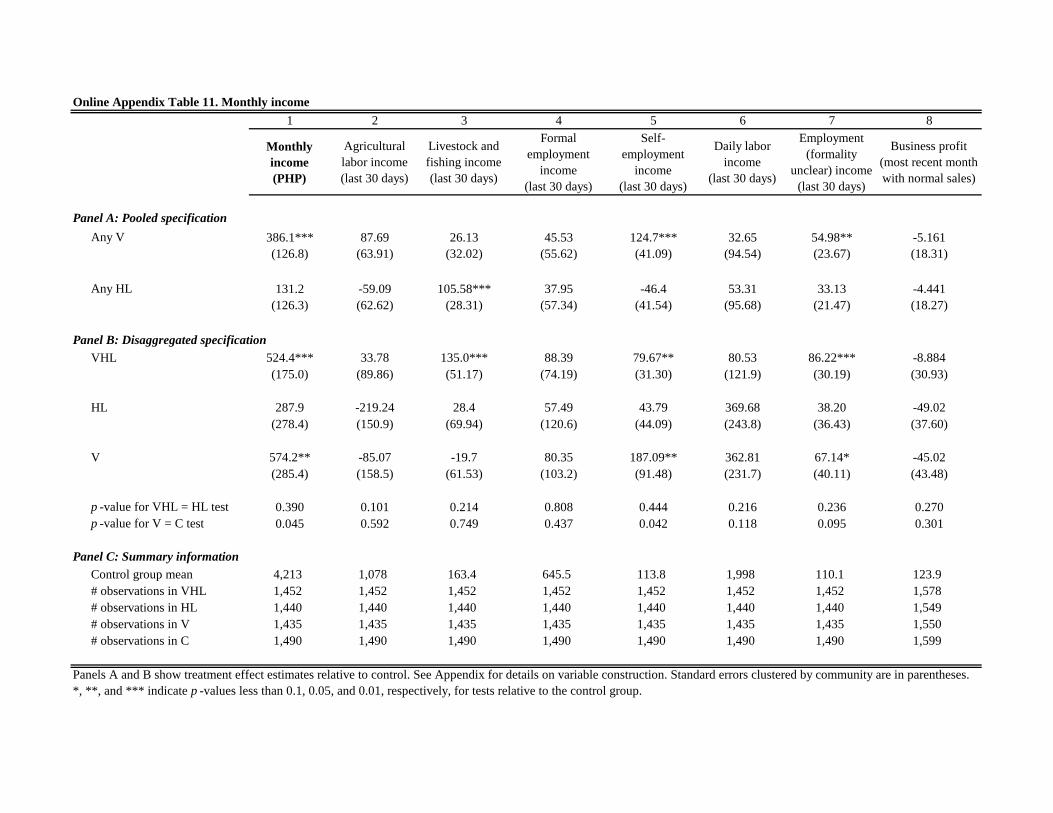
1 2 3 4 5 6 7 8
Monthly
income
(PHP)
Agricultural
labor income
(last 30 days)
Livestock and
fishing income
(last 30 days)
Formal
employment
income
(last 30 days)
Self-
employment
income
(last 30 days)
Daily labor
income
(last 30 days)
Employment
(formality
unclear) income
(last 30 days)
Business profit
(most recent month
with normal sales)
Panel A: Pooled specification
Any V 386.1*** 87.69 26.13 45.53 124.7*** 32.65 54.98** -5.161
(126.8) (63.91) (32.02) (55.62) (41.09) (94.54) (23.67) (18.31)
Any HL 131.2 -59.09 105.58*** 37.95 -46.4 53.31 33.13 -4.441
(126.3) (62.62) (28.31) (57.34) (41.54) (95.68) (21.47) (18.27)
Panel B: Disaggregated specification
VHL 524.4*** 33.78 135.0*** 88.39 79.67** 80.53 86.22*** -8.884
(175.0) (89.86) (51.17) (74.19) (31.30) (121.9) (30.19) (30.93)
HL 287.9 -219.24 28.4 57.49 43.79 369.68 38.20 -49.02
(278.4) (150.9) (69.94) (120.6) (44.09) (243.8) (36.43) (37.60)
V 574.2** -85.07 -19.7 80.35 187.09** 362.81 67.14* -45.02
(285.4) (158.5) (61.53) (103.2) (91.48) (231.7) (40.11) (43.48)
p -value for VHL = HL test 0.390 0.101 0.214 0.808 0.444 0.216 0.236 0.270
p -value for V = C test 0.045 0.592 0.749 0.437 0.042 0.118 0.095 0.301
Panel C: Summary information
Control group mean 4,213 1,078 163.4 645.5 113.8 1,998 110.1 123.9
# observations in VHL 1,452 1,452 1,452 1,452 1,452 1,452 1,452 1,578
# observations in HL 1,440 1,440 1,440 1,440 1,440 1,440 1,440 1,549
# observations in V 1,435 1,435 1,435 1,435 1,435 1,435 1,435 1,550
# observations in C 1,490 1,490 1,490 1,490 1,490 1,490 1,490 1,599
Online Appendix Table 11. Monthly income
Panels A and B show treatment effect estimates relative to control. See Appendix for details on variable construction. Standard errors clustered by community are in parentheses.
*, **, and *** indicate p -values less than 0.1, 0.05, and 0.01, respectively, for tests relative to the control group.

1 2 3 4 5 6 7
Adult weekly
labor supply
(hours)
Hours in
agricultural labor
(last 7 days)
Hours in livestock
and fishing
(last 7 days)
Hours in formal
employment
(last 7 days)
Hours in self
employment
(last 7 days)
Hours in
daily labor
(last 7 days)
Hours in
employment with
unclear formality
(last 7 days)
Panel A: Pooled specification
Any V 0.926 -2.072* 0.776* -0.114 0.986*** 0.806 0.544**
(1.091) (1.149) (0.439) (0.563) (0.272) (1.141) (0.234)
Any HL -1.822* -1.534 0.809* -0.818 -0.350 -0.192 0.264
(1.095) (1.147) (0.420) (0.587) (0.269) (1.144) (0.225)
Panel B: Disaggregated specification
VHL -0.878 -3.584** 1.598** -0.889 0.634** 0.565 0.799**
(1.417) (1.407) (0.636) (0.842) (0.311) (1.476) (0.338)
HL -0.149 -2.394 0.550 -1.057 0.429 2.371 -0.047
(2.390) (3.158) (0.973) (1.357) (0.483) (2.842) (0.395)
V 2.951 -3.469 1.163 -0.280 1.596** 3.652 0.290
(2.321) (3.096) (1.253) (1.320) (0.624) (2.748) (0.393)
p -value for VHL = HL test 0.761 0.707 0.342 0.898 0.696 0.515 0.053
p -value for V = C test 0.204 0.263 0.354 0.832 0.011 0.185 0.461
Panel C: Summary information
Control group mean 79.58 26.66 3.016 10.21 1.856 35.93 1.912
# observations in VHL 1,452 1,452 1,452 1,452 1,452 1,452 1,452
# observations in HL 1,439 1,439 1,439 1,439 1,439 1,439 1,439
# observations in V 1,434 1,434 1,434 1,434 1,434 1,434 1,434
# observations in C 1,490 1,490 1,490 1,490 1,490 1,490 1,490
Online Appendix Table 12. Adult labor supply
Panels A and B show treatment effect estimates relative to control. Dependent variables are indicated in the column title. See Appendix for details on
variable construction. Standard errors clustered by community are in parentheses. *, **, and *** indicate p -values less than 0.1, 0.05, and 0.01,
respectively, for tests relative to the control group.

1 2 3 4 5 6 7 8 9 10 11 12
Life
satisfaction
index
Kessler K6
nonspecific
distress scale
Nervous HopelessRestless or
fidgety
So depressed
that nothing
could you cheer
you up
That
everything
was
difficult
Worthless
How would
you describe
your
satisfaction
with life?
Taking all
things
together,
would you
say you are
happy?
Did you experience the
following feelings
during a lot of the day
yesterday? Enjoyment +
happiness - worry -
sadness
Did you smile
or laugh a lot
yesterday?
Panel A: Pooled specification
Any V 0.019 0.078 0.030 0.020 -0.052** -0.048** 0.018 0.057*** -0.123* 0.030** -0.006 0.009
(0.022) (0.100) (0.023) (0.021) (0.025) (0.024) (0.026) (0.020) (0.073) (0.012) (0.026) (0.006)
Any HL -0.010 0.291*** 0.069*** 0.004 0.064*** 0.048** 0.057** 0.027 -0.176** -0.021* 0.017 -0.004
(0.022) (0.099) (0.022) (0.022) (0.024) (0.023) (0.026) (0.020) (0.075) (0.012) (0.026) (0.006)
Panel B: Disaggregated specification
VHL 0.009 0.385*** 0.100*** 0.026 0.015 0.003 0.079** 0.088*** -0.301*** 0.009 0.009 0.004
(0.028) (0.123) (0.031) (0.025) (0.030) (0.031) (0.031) (0.029) (0.098) (0.015) (0.037) (0.009)
HL -0.031 0.314 0.040 -0.010 0.056 0.069 0.058 0.043 -0.161 -0.026 -0.016 -0.014
(0.056) (0.264) (0.050) (0.050) (0.066) (0.054) (0.072) (0.046) (0.161) (0.031) (0.058) (0.014)
V -0.018 0.058 -0.000 -0.009 -0.063 -0.038 0.019 0.070 -0.187 0.022 -0.039 -0.003
(0.047) (0.250) (0.048) (0.050) (0.060) (0.052) (0.064) (0.045) (0.156) (0.025) (0.056) (0.013)
p -value for VHL = HL test 0.478 0.789 0.227 0.474 0.529 0.238 0.768 0.330 0.380 0.255 0.669 0.240
p -value for V = C test 0.708 0.816 0.995 0.859 0.292 0.463 0.766 0.125 0.234 0.370 0.491 0.836
Panel C: Summary information
Control group mean 0 21.50 3.127 3.950 3.464 3.836 3.045 4.242 5.666 3.134 0.420 0.897
# observations in VHL 1,578 1,577 1,574 1,569 1,571 1,569 1,571 1,568 1,575 1,562 1,578 1,578
# observations in HL 1,549 1,549 1,547 1,540 1,543 1,541 1,543 1,534 1,547 1,534 1,549 1,549
# observations in V 1,550 1,550 1,550 1,548 1,545 1,543 1,541 1,539 1,548 1,539 1,550 1,550
# observations in C 1,599 1,598 1,593 1,580 1,594 1,588 1,589 1,575 1,598 1,588 1,599 1,599
Online Appendix Table 13. Life satisfaction index
Panels A and B show treatment effect estimates relative to control. Dependent variables are indicated in the column title. Variables have been coded so that more positive numbers correspond to less
psychological distress and higher life satisfaction. See Appendix for details on variable construction. The variables to the right of the first column have not been standardized. Standard errors clustered by
community are in parentheses. *, **, and *** indicate p -values less than 0.1, 0.05, and 0.01, respectively, for tests relative to the control group.
About how often during the past 30 days did you feel…

1
Where would you place your
household on the ladder in terms of
economic status?
Panel A: Pooled specification
Any V -0.113**
(0.047)
Any HL -0.040
(0.047)
Panel B: Disaggregated specification
VHL -0.151**
(0.067)
HL -0.073
(0.112)
V -0.133
(0.119)
p -value for VHL = HL test 0.488
p -value for V = C test 0.264
Panel C: Summary information
Control group mean 3.242
# observations in VHL 1,576
# observations in HL 1,548
# observations in V 1,547
# observations in C 1,596
Online Appendix Table 14. Perceived relative economic status
Panels A and B show treatment effect estimates relative to control. The dependent variable,
indicated in the column title, has been coded so that more positive numbers correspond to
higher perceived relative economic status. See Appendix for details on variable
construction. Standard errors clustered by community are in parentheses. *, **, and ***
indicate p -values less than 0.1, 0.05, and 0.01, respectively, for tests relative to the control
group.

Online Appendix Table 15. Trust index
1 2 3 4
Trust index
In general, would
you say that most
people can be trusted
or that most people
cannot be trusted?
Do you think most
people would try to take
advantage of you if they
got a chance, or would
they try to be fair?
Would you say that most
of the time people try to
be helpful, or that they
are mostly just looking
out for themselves?
Panel A: Pooled specification
Any V 0.004 0.00 0.005 -0.001
(0.022) (0.010) (0.010) (0.011)
Any HL -0.023 -0.003 -0.002 -0.021**
(0.022) (0.010) (0.009) (0.011)
Panel B: Disaggregated specification
VHL -0.019 -0.003 0.003 -0.021
(0.032) (0.015) (0.014) (0.015)
HL -0.023 0.000 0.003 -0.030
(0.043) (0.019) (0.020) (0.022)
V -0.018 -0.005 -0.002 -0.013
(0.046) (0.021) (0.022) (0.021)
p -value for VHL = HL test 0.927 0.870 0.986 0.718
p -value for V = C test 0.704 0.811 0.932 0.533
Panel C: Summary information
Control group mean 0 0.458 0.637 0.582
# observations in VHL 1,578 1,578 1,578 1,578
# observations in HL 1,549 1,549 1,549 1,549
# observations in V 1,550 1,550 1,550 1,550
# observations in C 1,599 1,599 1,599 1,599
Panels A and B show treatment effect estimates relative to control. Dependent variables are indicated in the column title.
Variables have been coded so that more positive numbers correspond to more trust. See Appendix for details on variable
construction. The variables to the right of the first column have not been standardized. Standard errors clustered by community
are in parentheses. *, **, and *** indicate p -values less than 0.1, 0.05, and 0.01, respectively, for tests relative to the control
group.

Online Appendix Table 16. Social safety net index
1 2 3 4 5 6 7 8 9
Social safety
net index
Likelihood that
could access 40
PHP from a source
outside household
for urgent need
Likelihood that
could access 1,000
PHP from a source
outside household
for urgent need
Do you discuss
personal issues with
anyone outside
your close family?
How often do you
usually speak to
this person?
(number of days in
a year)
Household
received meals
from another
household in local
community (last
30 days)
Number of
meals
received
Household gave
meals to another
household in
local community
(last 30 days)
Number
of meals
given
Panel A: Pooled specification
Any V 0.026 0.018 -0.025 0.020 0.250 0.004 0.344** 0.000 0.193
(0.024) (0.025) (0.033) (0.012) (0.573) (0.011) (0.162) (0.011) (0.182)
Any HL -0.027 -0.028 0.044 -0.001 0.165 -0.003 -0.264 -0.010 -0.539***
(0.024) (0.026) (0.033) (0.012) (0.570) (0.010) (0.164) (0.011) (0.185)
Panel B: Disaggregated specification
VHL -0.000 -0.011 0.020 0.018 0.424 0.001 0.089 -0.010 -0.337
(0.032) (0.033) (0.044) (0.016) (0.782) (0.014) (0.205) (0.015) (0.267)
HL -0.076 -0.064 -0.009 0.004 -0.045 -0.036 -0.393 -0.036 -0.429
(0.048) (0.053) (0.071) (0.021) (1.287) (0.024) (0.333) (0.025) (0.472)
V -0.023 -0.023 -0.071 0.025 -0.075 -0.022 0.206 -0.026 0.081
(0.048) (0.053) (0.072) (0.024) (1.109) (0.022) (0.386) (0.023) (0.494)
p -value for VHL = HL test 0.140 0.346 0.692 0.496 0.696 0.136 0.159 0.302 0.846
p -value for V = C test 0.631 0.662 0.323 0.292 0.946 0.331 0.594 0.246 0.870
Panel C: Summary information
Control group mean 0 3.617 2.359 0.387 8.480 0.557 4.497 0.683 5.260
# observations in VHL 1,578 1,578 1,578 1,552 1,530 1,535 1,531 1,536 1,489
# observations in HL 1,549 1,549 1,549 1,538 1,518 1,528 1,525 1,520 1,471
# observations in V 1,550 1,550 1,550 1,528 1,504 1,517 1,510 1,504 1,463
# observations in C 1,599 1,599 1,599 1,583 1,551 1,570 1,551 1,563 1,525
Panels A and B show treatment effect estimates relative to control. Dependent variables are indicated in the column title. Variables have been coded so that more positive numbers correspond to
more access to a social safety net. See Appendix for details on variable construction. The variables to the right of the first column have not been standardized. Standard errors clustered by
community are in parentheses. *, **, and *** indicate p -values less than 0.1, 0.05, and 0.01, respectively, for tests relative to the control group.

Online Appendix Table 17. Community activities index
1 2 3 4
Commmunity
activities index
Did you attend any
village leaders
meetings?
(last 6 months)
Have you
participated in any
community
activities?
(last 6 months)
How frequently did
you participate in
community
activities? (number
of days in a year)
Panel A: Pooled specification
Any V 0.005 -0.019* 0.007 0.666
(0.025) (0.011) (0.013) (0.510)
Any HL 0.041 -0.001 0.014 1.354***
(0.025) (0.011) (0.012) (0.507)
Panel B: Disaggregated specification
VHL 0.045 -0.020 0.021 1.998**
(0.034) (0.015) (0.016) (0.800)
HL 0.019 -0.024 0.011 1.658*
(0.058) (0.025) (0.031) (0.996)
V -0.011 -0.043* 0.009 1.126
(0.059) (0.026) (0.031) (0.975)
p -value for VHL = HL test 0.655 0.852 0.750 0.748
p -value for V = C test 0.857 0.094 0.771 0.249
Panel C: Summary information
Control group mean 0 0.651 0.527 9.165
# observations in VHL 1,561 1,554 1,546 1,533
# observations in HL 1,542 1,540 1,533 1,523
# observations in V 1,534 1,532 1,525 1,516
# observations in C 1,592 1,589 1,580 1,561
Panels A and B show treatment effect estimates relative to control. Dependent variables are indicated in the column
title. Variables have been coded so that more positive numbers correspond to more involvement in community
activities. See Appendix for details on variable construction. The variables to the right of the first column have not
been standardized. Standard errors clustered by community are in parentheses. *, **, and *** indicate p -values less
than 0.1, 0.05, and 0.01, respectively, for tests relative to the control group.

Online Appendix Table 18. Perceived stress scale index
1 2 3 4 5
Perceived stress
scale index
How often have you
felt that you were
unable to control the
important things in
your life?
How often have you felt
confident about your
ability to handle your
personal problems?
How often have
you felt that things
were going your
way?
How often have
you felt difficulties
were piling up so
high that you could
not overcome
them?
Panel A: Pooled specification
Any V -0.011 0.055** -0.065*** -0.024 -0.005
(0.020) (0.023) (0.023) (0.022) (0.025)
Any HL -0.018 -0.015 0.005 -0.049** 0.022
(0.021) (0.023) (0.024) (0.022) (0.025)
Panel B: Disaggregated specification
VHL -0.026 0.042 -0.061* -0.072** 0.021
(0.026) (0.036) (0.035) (0.030) (0.033)
HL -0.009 0.069 -0.016 -0.079 0.010
(0.044) (0.057) (0.056) (0.054) (0.052)
V -0.007 0.118** -0.064 -0.044 -0.035
(0.043) (0.057) (0.052) (0.049) (0.053)
p -value for VHL = HL test 0.684 0.650 0.434 0.901 0.843
p -value for V = C test 0.876 0.038 0.216 0.368 0.509
Panel C: Summary information
Control group mean 0 2.896 3.430 2.936 3.265
# observations in VHL 1,577 1,572 1,574 1,567 1,569
# observations in HL 1,549 1,543 1,543 1,536 1,539
# observations in V 1,549 1,544 1,543 1,538 1,545
# observations in C 1,599 1,596 1,593 1,583 1,590
Panels A and B show treatment effect estimates relative to control. Dependent variables are indicated in the column title. Variables have been coded so that more
positive numbers correspond to less stress. See Appendix for details on variable construction. The variables to the right of the first column have not been
standardized. Standard errors clustered by community are in parentheses. *, **, and *** indicate p -values less than 0.1, 0.05, and 0.01, respectively, for tests
relative to the control group.

1 2 3 4 5 6 7
Powerful
others index
I feel like what
happens in my life
is mostly
determined by God
Although I might
have good ability, I
will not be
successful without
appealing to God
My life is
chiefly
controlled by
God
Getting what I
want requires
pleasing God
Whether or not I
have an accident
and hurt myself
physically depends
mostly on God
In order to have my
plans work, I make
sure that they fit
with God’s plan for
me
Panel A: Pooled specification
Any V 0.093*** 0.109*** 0.030* 0.088*** 0.022 0.049 0.057***
(0.027) (0.024) (0.017) (0.022) (0.023) (0.031) (0.019)
Any HL 0.044 0.021 0.026 0.044** 0.007 0.016 0.052***
(0.027) (0.024) (0.017) (0.022) (0.023) (0.032) (0.019)
Panel B: Disaggregated specification
VHL 0.135*** 0.128*** 0.054*** 0.131*** 0.028 0.066 0.108***
(0.038) (0.035) (0.020) (0.032) (0.032) (0.047) (0.027)
HL 0.031 0.037 -0.025 0.060 -0.031 0.029 0.046
(0.060) (0.051) (0.037) (0.052) (0.048) (0.073) (0.041)
V 0.073 0.118** -0.016 0.095* -0.019 0.048 0.051
(0.059) (0.048) (0.036) (0.048) (0.048) (0.071) (0.042)
p -value for VHL = HL test 0.085 0.068 0.033 0.175 0.246 0.614 0.123
p -value for V = C test 0.222 0.015 0.659 0.050 0.689 0.501 0.229
Panel C: Summary information
Control group mean 0 4.271 4.612 4.388 4.458 3.907 4.502
# observations in VHL 1,578 1,578 1,578 1,578 1,578 1,578 1,578
# observations in HL 1,549 1,549 1,549 1,549 1,549 1,549 1,549
# observations in V 1,550 1,550 1,550 1,550 1,550 1,550 1,550
# observations in C 1,599 1,599 1,599 1,599 1,599 1,599 1,599
Online Appendix Table 19. Powerful others index
Panels A and B show treatment effect estimates relative to control. Dependent variables are indicated in the column title. Variables have been coded so that more
positive numbers correspond to higher perception of God’s role in determining outcomes in life. See Appendix for details on variable construction. The variables to the
right of the first column have not been standardized. Standard errors clustered by community are in parentheses. *, **, and *** indicate p -values less than 0.1, 0.05, and
0.01, respectively, for tests relative to the control group.

1 2 3 4 5 6 7 8 9 10
Locus of
control
index
Internality
subscale
Whether or
not I am
successful
depends
mostly on my
ability
Whether or not I
have an accident
and hurt myself
depends mostly
on how careful I
am on a daily
basis
When I make
plans, I am
almost
certain to
make them
work
How many
friends I
have
depends on
how nice a
person I am
I can pretty
much
determine
what will
happen in
my life
I am usually
able to
protect my
personal
interests
When I get
what I want
it’s usually
because I
worked hard
for it
My life is
determined
by my own
actions
Panel A: Pooled specification
Any V -0.035* 0.088*** 0.091*** 0.015 0.070** 0.009 0.084** 0.041 0.047*** 0.014
(0.020) (0.026) (0.020) (0.021) (0.033) (0.017) (0.036) (0.028) (0.015) (0.019)
Any HL -0.000 -0.019 -0.023 -0.013 -0.018 -0.017 0.024 -0.006 0.015 -0.040**
(0.020) (0.026) (0.021) (0.021) (0.031) (0.017) (0.036) (0.028) (0.015) (0.018)
Panel B: Disaggregated specification
VHL -0.035 0.069* 0.068** 0.001 0.051 -0.008 0.108** 0.035 0.060*** -0.026
(0.029) (0.035) (0.031) (0.032) (0.040) (0.021) (0.050) (0.035) (0.020) (0.027)
HL -0.064 0.002 0.028 -0.022 0.087 -0.042 0.014 -0.033 -0.006 -0.017
(0.057) (0.060) (0.046) (0.042) (0.081) (0.039) (0.086) (0.069) (0.034) (0.038)
V -0.085* 0.103* 0.145*** 0.001 0.175** -0.022 0.067 0.011 0.025 0.033
(0.050) (0.056) (0.042) (0.043) (0.078) (0.038) (0.084) (0.066) (0.033) (0.038)
p -value for VHL = HL test 0.605 0.298 0.393 0.586 0.666 0.389 0.312 0.326 0.044 0.831
p -value for V = C test 0.090 0.067 0.001 0.974 0.026 0.562 0.425 0.869 0.439 0.383
Panel C: Summary information
Control group mean 0 0 4.218 4.123 3.108 4.510 2.333 3.402 4.578 4.309
# observations in VHL 1,578 1,578 1,578 1,578 1,578 1,578 1,578 1,578 1,578 1,578
# observations in HL 1,549 1,549 1,549 1,549 1,549 1,549 1,549 1,549 1,549 1,549
# observations in V 1,550 1,550 1,550 1,550 1,550 1,550 1,550 1,550 1,550 1,550
# observations in C 1,599 1,599 1,599 1,599 1,599 1,599 1,599 1,599 1,599 1,599
Online Appendix Table 20a: Locus of control index: Internality subscale
Panels A and B show treatment effect estimates relative to control. Dependent variables are indicated in the column title. Variables have been coded so that more positive
numbers correspond to higher perceptions of people’s ability to control their life/fate. See Appendix for details on variable construction. The variables to the right of the second
column have not been standardized. Standard errors clustered by community are in parentheses. *, **, and *** indicate p -values less than 0.1, 0.05, and 0.01, respectively, for
tests relative to the control group.

11 12 13 14 15 16 17 18 19 20
Chance
subscale
To a great
extent my
life is
controlled
by
accidental
happenings
Often there is no
chance of
protecting my
personal interests
from bad luck
happening
When I get
what I want,
it is usually
because I am
lucky
I have often
found that
what is going
to happen
will happen
Whether or not
I get into an
accident and
hurt myself
physically is
mostly a matter
of luck
It is not wise for
me to plan too
far ahead
because many
things turn out
to be a matter of
good or bad
fortune
Whether or not I
am successful
depends on
whether I am
lucky enough to
be in the right
place at the right
time
It is chiefly a
matter of
fate whether
or not I have
a few friends
or many
friends
Closest to your view on
a scale on which (1)
“everything in life is
determined by fate” and
(10) “people shape their
fate themselves”
Panel A: Pooled specification
Any V -0.098*** -0.135*** -0.046 -0.075*** -0.058 -0.025 -0.101*** -0.029 -0.127*** -0.192**
(0.028) (0.032) (0.028) (0.028) (0.038) (0.030) (0.037) (0.026) (0.032) (0.079)
Any HL 0.004 -0.006 -0.019 0.008 -0.016 -0.026 0.016 0.010 0.057* 0.060
(0.028) (0.032) (0.028) (0.028) (0.039) (0.030) (0.037) (0.027) (0.032) (0.080)
Panel B: Disaggregated specification
VHL -0.094** -0.141*** -0.065* -0.065* -0.075 -0.051 -0.084 -0.019 -0.069* -0.128
(0.038) (0.049) (0.037) (0.038) (0.050) (0.043) (0.055) (0.036) (0.041) (0.118)
HL -0.064 -0.044 -0.090 0.014 -0.053 -0.050 -0.078 -0.012 -0.074 -0.168
(0.076) (0.102) (0.073) (0.077) (0.082) (0.067) (0.090) (0.059) (0.102) (0.204)
V -0.157** -0.152 -0.117 -0.072 -0.102 -0.046 -0.190** -0.057 -0.219** -0.343*
(0.075) (0.103) (0.073) (0.069) (0.082) (0.071) (0.087) (0.057) (0.099) (0.181)
p -value for VHL = HL test 0.708 0.343 0.738 0.313 0.796 0.992 0.945 0.909 0.958 0.843
p -value for V = C test 0.036 0.140 0.110 0.297 0.216 0.512 0.029 0.317 0.028 0.060
Panel C: Summary information
Control group mean 0 2.704 2.749 2.412 3.074 2.786 2.994 2.061 2.463 5.907
# observations in VHL 1,578 1,578 1,578 1,578 1,578 1,578 1,578 1,578 1,578 1,578
# observations in HL 1,549 1,549 1,549 1,549 1,549 1,549 1,549 1,549 1,549 1,549
# observations in V 1,550 1,550 1,550 1,550 1,550 1,550 1,550 1,550 1,550 1,549
# observations in C 1,599 1,599 1,599 1,599 1,599 1,599 1,599 1,599 1,599 1,599
Online Appendix Table 20b. Locus of control index: Chance subscale and World Values Survey question
Panels A and B show treatment effect estimates relative to control. Dependent variables are indicated in the column title. Variables have been coded so that more positive numbers correspond to lower
perception of chance’s ability to determine outcomes in life. See Appendix for details on variable construction. The variables to the right of the first column have not been standardized. Standard
errors clustered by community are in parentheses. *, **, and *** indicate p -values less than 0.1, 0.05, and 0.01, respectively, for tests relative to the control group.
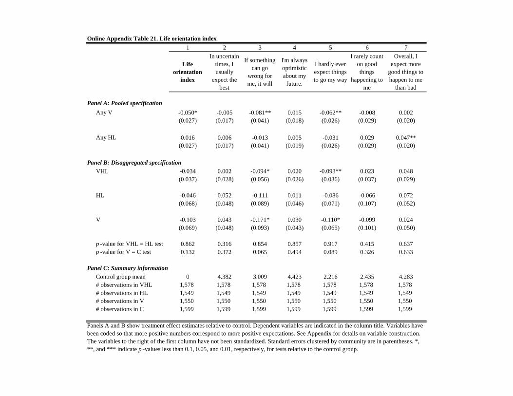
1 2 3 4 5 6 7
Life
orientation
index
In uncertain
times, I
usually
expect the
best
If something
can go
wrong for
me, it will
I'm always
optimistic
about my
future.
I hardly ever
expect things
to go my way
I rarely count
on good
things
happening to
me
Overall, I
expect more
good things to
happen to me
than bad
Panel A: Pooled specification
Any V -0.050* -0.005 -0.081** 0.015 -0.062** -0.008 0.002
(0.027) (0.017) (0.041) (0.018) (0.026) (0.029) (0.020)
Any HL 0.016 0.006 -0.013 0.005 -0.031 0.029 0.047**
(0.027) (0.017) (0.041) (0.019) (0.026) (0.029) (0.020)
Panel B: Disaggregated specification
VHL -0.034 0.002 -0.094* 0.020 -0.093** 0.023 0.048
(0.037) (0.028) (0.056) (0.026) (0.036) (0.037) (0.029)
HL -0.046 0.052 -0.111 0.011 -0.086 -0.066 0.072
(0.068) (0.048) (0.089) (0.046) (0.071) (0.107) (0.052)
V -0.103 0.043 -0.171* 0.030 -0.110* -0.099 0.024
(0.069) (0.048) (0.093) (0.043) (0.065) (0.101) (0.050)
p -value for VHL = HL test 0.862 0.316 0.854 0.857 0.917 0.415 0.637
p -value for V = C test 0.132 0.372 0.065 0.494 0.089 0.326 0.633
Panel C: Summary information
Control group mean 0 4.382 3.009 4.423 2.216 2.435 4.283
# observations in VHL 1,578 1,578 1,578 1,578 1,578 1,578 1,578
# observations in HL 1,549 1,549 1,549 1,549 1,549 1,549 1,549
# observations in V 1,550 1,550 1,550 1,550 1,550 1,550 1,550
# observations in C 1,599 1,599 1,599 1,599 1,599 1,599 1,599
Online Appendix Table 21. Life orientation index
Panels A and B show treatment effect estimates relative to control. Dependent variables are indicated in the column title. Variables have
been coded so that more positive numbers correspond to more positive expectations. See Appendix for details on variable construction.
The variables to the right of the first column have not been standardized. Standard errors clustered by community are in parentheses. *,
**, and *** indicate p -values less than 0.1, 0.05, and 0.01, respectively, for tests relative to the control group.

1 2 3 4 5 6
Expectations
index
Which step of the
life satisfaction
ladder do you
believe you will be
on in 5 years?
Where do you think you
will be on the relative
economic status ladder
5 years from now?
Optimism
index
How optimistic are
you in general, on a
scale of 1 to 7?
How pessimistic
are you in general,
on a scale of 1 to 7?
Panel A: Pooled specification
Any V -0.037 -0.014 -0.136** 0.053** 0.056 0.100**
(0.025) (0.065) (0.059) (0.024) (0.039) (0.042)
Any HL -0.016 -0.032 -0.026 -0.024 -0.022 -0.049
(0.025) (0.069) (0.059) (0.024) (0.038) (0.042)
Panel B: Disaggregated specification
VHL -0.055* -0.054 -0.160** 0.030 0.036 0.051
(0.032) (0.090) (0.076) (0.032) (0.047) (0.062)
HL -0.014 0.006 -0.010 -0.007 -0.076 0.057
(0.056) (0.139) (0.147) (0.061) (0.105) (0.096)
V -0.054 -0.084 -0.119 0.069 0.001 0.203**
(0.057) (0.148) (0.140) (0.066) (0.116) (0.099)
p -value for VHL = HL test 0.468 0.672 0.314 0.541 0.276 0.955
p -value for V = C test 0.344 0.569 0.393 0.298 0.990 0.040
Panel C: Summary information
Control group mean 0 6.743 4.834 0 5.544 5.398
# observations in VHL 1,542 1,500 1,474 1,578 1,578 1,578
# observations in HL 1,508 1,467 1,444 1,549 1,549 1,549
# observations in V 1,518 1,480 1,465 1,550 1,550 1,550
# observations in C 1,567 1,541 1,494 1,599 1,599 1,599
Online Appendix Table 22. Expectations index and optimism index
Panels A and B show treatment effect estimates relative to control. Dependent variables are indicated in the column title. Variables have been coded so that
more positive numbers correspond to higher optimism. See Appendix for details on variable construction. The variables in the second, third, fourth, and
fifth columns have not been standardized. Standard errors clustered by community are in parentheses. *, **, and *** indicate p -values less than 0.1, 0.05,
and 0.01, respectively, for tests relative to the control group.

1 2 3 4 5 6 7 8 9
Grit index
New ideas and
projects
sometimes
distract me
from previous
ones
Setbacks don't
discourage me
I have been
obsessed with
a certain idea
or project for a
short time but
later lost
interest
I am a very
hard worker
I often set a
goal but later
choose to
pursue a
different one
I have
difficulty
maintaining my
focus on
projects that
take more than
a few months
I finish
whatever I
begin
I am diligent
Panel A: Pooled specification
Any V 0.041* -0.011 0.075*** -0.006 0.082*** -0.040 -0.013 0.059*** 0.026
(0.022) (0.029) (0.025) (0.025) (0.019) (0.029) (0.025) (0.021) (0.018)
Any HL 0.017 0.015 -0.030 0.020 0.002 0.006 0.072*** 0.001 -0.014
(0.022) (0.028) (0.025) (0.025) (0.019) (0.029) (0.024) (0.021) (0.017)
Panel B: Disaggregated specification
VHL 0.056* 0.005 0.040 0.015 0.084*** -0.036 0.059* 0.058** 0.011
(0.029) (0.037) (0.035) (0.030) (0.027) (0.037) (0.032) (0.028) (0.025)
HL 0.030 0.024 -0.075 0.048 0.006 -0.019 0.105* 0.029 0.010
(0.058) (0.069) (0.057) (0.061) (0.041) (0.069) (0.063) (0.052) (0.042)
V 0.041 -0.011 0.036 -0.004 0.082** -0.082 -0.004 0.098** 0.057
(0.058) (0.075) (0.058) (0.063) (0.041) (0.065) (0.062) (0.048) (0.040)
p -value for VHL = HL test 0.671 0.782 0.045 0.591 0.064 0.809 0.474 0.587 0.974
p -value for V = C test 0.484 0.882 0.528 0.954 0.046 0.211 0.953 0.043 0.156
Panel C: Summary information
Control group mean 0 3.148 3.499 3.120 4.241 3.193 3.071 4.249 4.422
# observations in VHL 1,578 1,578 1,578 1,578 1,578 1,578 1,578 1,578 1,578
# observations in HL 1,549 1,549 1,549 1,549 1,549 1,549 1,549 1,549 1,549
# observations in V 1,550 1,550 1,550 1,550 1,550 1,550 1,550 1,550 1,550
# observations in C 1,599 1,599 1,599 1,599 1,599 1,599 1,599 1,599 1,599
Online Appendix Table 23. Grit index
Panels A and B show treatment effect estimates relative to control. Dependent variables are indicated in the column title. Variables have been coded so that more positive numbers
correspond to more grit. See Appendix for details on variable construction. The variables to the right of the first column have not been standardized. Standard errors clustered by
community are in parentheses. *, **, and *** indicate p -values less than 0.1, 0.05, and 0.01, respectively, for tests relative to the control group.

1 2 3 4 5 6 7 8 9 10 11
Self control
index
I have a
hard time
breaking
bad habits
I get
distracted
easily
I say
inappropriate
things
I refuse
things that
are bad for
me, even if
they are fun.
I'm good at
resisting
temptation
People
would say
that I have
very strong
self-
discipline
Pleasure
and fun
sometimes
keep me
from getting
work done
I do things
that feel
good in the
moment but
regret later
on
Sometimes I
can't stop
myself from
doing
something,
even if I know
it's wrong
I often act
without
thinking
through all
the
alternatives
Panel A: Pooled specification
Any V -0.034* -0.043 -0.003 -0.026 0.019 -0.097*** -0.060** 0.014 -0.041 -0.004 -0.008
(0.021) (0.026) (0.026) (0.030) (0.026) (0.029) (0.027) (0.026) (0.028) (0.029) (0.028)
Any HL 0.006 -0.036 -0.023 -0.020 0.039 -0.008 0.009 0.054** 0.008 0.027 -0.008
(0.020) (0.026) (0.026) (0.030) (0.026) (0.029) (0.027) (0.026) (0.028) (0.029) (0.028)
Panel B: Disaggregated specification
VHL -0.027 -0.076** -0.026 -0.045 0.057 -0.103** -0.050 0.068** -0.028 0.026 -0.015
(0.025) (0.037) (0.039) (0.037) (0.038) (0.040) (0.036) (0.030) (0.034) (0.038) (0.032)
HL 0.039 -0.046 -0.030 -0.022 0.060 0.019 0.005 0.153** 0.063 0.073 0.008
(0.047) (0.062) (0.065) (0.067) (0.077) (0.079) (0.069) (0.068) (0.064) (0.056) (0.064)
V -0.001 -0.050 -0.018 -0.026 0.018 -0.062 -0.050 0.100 0.019 0.049 0.012
(0.050) (0.063) (0.061) (0.072) (0.078) (0.081) (0.065) (0.073) (0.063) (0.056) (0.066)
p -value for VHL = HL test 0.155 0.615 0.957 0.728 0.962 0.103 0.436 0.198 0.153 0.442 0.722
p -value for V = C test 0.980 0.429 0.772 0.717 0.819 0.444 0.440 0.171 0.768 0.384 0.855
Panel C: Summary information
Control group mean 0 3.032 2.863 3.014 3.135 3.358 3.219 3.136 2.947 2.961 2.946
# observations in VHL 1,578 1,578 1,578 1,578 1,578 1,578 1,578 1,578 1,578 1,578 1,578
# observations in HL 1,549 1,549 1,549 1,549 1,549 1,549 1,549 1,549 1,549 1,549 1,549
# observations in V 1,550 1,550 1,550 1,550 1,550 1,550 1,550 1,550 1,550 1,550 1,550
# observations in C 1,599 1,599 1,599 1,599 1,599 1,599 1,599 1,599 1,599 1,599 1,599
Online Appendix Table 24. Self-control index
Panels A and B show treatment effect estimates relative to control. Dependent variables are indicated in the column title. Variables have been coded so that more positive numbers
correspond to more self-control. See Appendix for details on variable construction. The variables to the right of the first column have not been standardized. Standard errors clustered
by community are in parentheses. *, **, and *** indicate p -values less than 0.1, 0.05, and 0.01, respectively, for tests relative to the control group.

1 2 3 4
Salvation by grace
belief index
If I am good enough,
God will cleanse me
of my sins
I follow God’s laws so
that I can go to heaven
I will go to heaven
because I have accepted
Jesus Christ as my
personal savior
Panel A: Pooled specification
Any V -0.036* -0.059*** -0.052*** 0.019*
(0.020) (0.020) (0.016) (0.011)
Any HL -0.005 -0.016 -0.006 0.003
(0.020) (0.020) (0.016) (0.011)
Panel B: Disaggregated specification
VHL -0.040 -0.073** -0.057*** 0.022
(0.026) (0.032) (0.022) (0.014)
HL -0.021 -0.060 -0.037 0.019
(0.045) (0.042) (0.039) (0.024)
V -0.061 -0.100** -0.085** 0.029
(0.041) (0.039) (0.036) (0.026)
p -value for VHL = HL test 0.696 0.792 0.616 0.901
p -value for V = C test 0.143 0.011 0.019 0.268
Panel C: Summary information
Control group mean 0 1.386 1.358 0.559
# observations in VHL 1,578 1,473 1,473 1,578
# observations in HL 1,549 1,457 1,457 1,549
# observations in V 1,550 1,455 1,455 1,550
# observations in C 1,599 1,515 1,515 1,599
Online Appendix Table 25. Salvation by grace belief index
Panels A and B show treatment effect estimates relative to control. Dependent variables are indicated in the column title.
Variables have been coded so that more positive numbers correspond to greater belief in the doctrine of salvation by grace. See
Appendix for details on variable construction. The variables to the right of the first column have not been standardized. Standard
errors clustered by community are in parentheses. *, **, and *** indicate p -values less than 0.1, 0.05, and 0.01, respectively, for
tests relative to the control group.
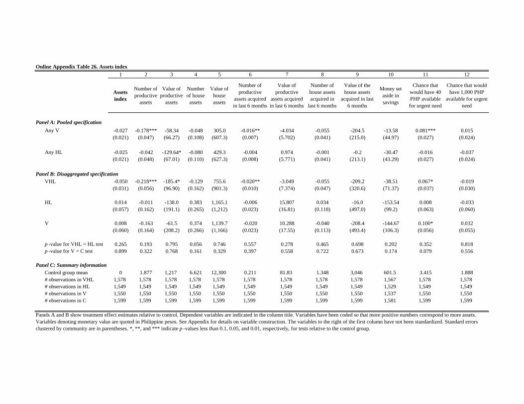
1 2 3 4 5 6 7 8 9 10 11 12
Assets
index
Number of
productive
assets
Value of
productive
assets
Number
of house
assets
Value of
house
assets
Number of
productive
assets acquired
in last 6 months
Value of
productive
assets acquired
in last 6 months
Number of
house assets
acquired in
last 6 months
Value of the
house assets
acquired in last
6 months
Money set
aside in
savings
Chance that
would have 40
PHP available
for urgent need
Chance that would
have 1,000 PHP
available for urgent
need
Panel A: Pooled specification
Any V -0.027 -0.178*** -58.34 -0.048 305.0 -0.016** -4.034 -0.055 -204.5 -13.58 0.081*** 0.015
(0.021) (0.047) (66.27) (0.108) (607.3) (0.007) (5.702) (0.041) (215.0) (44.97) (0.027) (0.024)
Any HL -0.025 -0.042 -129.64* -0.080 429.3 -0.004 0.974 -0.001 -0.2 -30.47 -0.016 -0.037
(0.021) (0.048) (67.01) (0.110) (627.3) (0.008) (5.771) (0.041) (213.1) (43.29) (0.027) (0.024)
Panel B: Disaggregated specification
VHL -0.050 -0.218*** -185.4* -0.129 755.6 -0.020** -3.049 -0.055 -209.2 -38.51 0.067* -0.019
(0.031) (0.056) (96.90) (0.162) (901.3) (0.010) (7.374) (0.047) (320.6) (71.37) (0.037) (0.030)
HL 0.014 -0.011 -138.0 0.383 1,165.1 -0.006 15.807 0.034 -16.0 -153.54 0.008 -0.033
(0.057) (0.162) (191.1) (0.265) (1,212) (0.023) (16.81) (0.118) (497.0) (99.2) (0.063) (0.060)
V 0.008 -0.163 -61.5 0.374 1,139.7 -0.020 10.288 -0.040 -208.4 -144.67 0.100* 0.032
(0.060) (0.164) (208.2) (0.266) (1,166) (0.023) (17.55) (0.113) (493.4) (106.3) (0.056) (0.055)
p -value for VHL = HL test 0.265 0.193 0.795 0.056 0.746 0.557 0.278 0.465 0.698 0.202 0.352 0.818
p -value for V = C test 0.899 0.322 0.768 0.161 0.329 0.397 0.558 0.722 0.673 0.174 0.079 0.556
Panel C: Summary information
Control group mean 0 1.877 1,217 6.621 12,300 0.211 81.83 1.348 3,046 601.5 3.415 1.888
# observations in VHL 1,578 1,578 1,578 1,578 1,578 1,578 1,578 1,578 1,578 1,567 1,578 1,578
# observations in HL 1,549 1,549 1,549 1,549 1,549 1,549 1,549 1,549 1,549 1,529 1,549 1,549
# observations in V 1,550 1,550 1,550 1,550 1,550 1,550 1,550 1,550 1,550 1,537 1,550 1,550
# observations in C 1,599 1,599 1,599 1,599 1,599 1,599 1,599 1,599 1,599 1,581 1,599 1,599
Online Appendix Table 26. Assets index
Panels A and B show treatment effect estimates relative to control. Dependent variables are indicated in the column title. Variables have been coded so that more positive numbers correspond to more assets.
Variables denoting monetary value are quoted in Philippine pesos. See Appendix for details on variable construction. The variables to the right of the first column have not been standardized. Standard errors
clustered by community are in parentheses. *, **, and *** indicate p -values less than 0.1, 0.05, and 0.01, respectively, for tests relative to the control group.

1 2 3 4
Financial
inclusion index
Do you or anyone in
your household
currently have money
set aside as savings?
Do you -- by yourself or
with other people --
currently have an
account at a bank?
Have you made a deposit
at a financial institution
in the past 6 months?
Panel A: Pooled specification
Any V 0.020 0.002 0.005 0.006
(0.024) (0.009) (0.009) (0.006)
Any HL 0.157*** 0.052*** 0.036*** 0.027***
(0.025) (0.010) (0.009) (0.006)
Panel B: Disaggregated specification
VHL 0.179*** 0.055*** 0.042*** 0.033***
(0.038) (0.015) (0.012) (0.009)
HL 0.124** 0.029 0.038* 0.019
(0.048) (0.024) (0.021) (0.013)
V -0.010 -0.025 0.014 -0.003
(0.044) (0.022) (0.018) (0.012)
p -value for VHL = HL test 0.297 0.288 0.852 0.300
p -value for V = C test 0.811 0.267 0.435 0.811
Panel C: Summary information
Control group mean 0 0.265 0.143 0.059
# observations in VHL 1,578 1,578 1,504 1,493
# observations in HL 1,549 1,549 1,486 1,456
# observations in V 1,550 1,550 1,482 1,459
# observations in C 1,599 1,599 1,522 1,507
Online Appendix Table 27. Financial inclusion index
Panels A and B show treatment effect estimates relative to control. Dependent variables are indicated in the column title. Variables
have been coded so that more positive numbers correspond to more financial inclusion. See Appendix for details on variable
construction. The variables to the right of the first column have not been standardized. Standard errors clustered by community are
in parentheses. *, **, and *** indicate p -values less than 0.1, 0.05, and 0.01, respectively, for tests relative to the control group.

1 2 3 4
Health index
Negative of number
of serious health
events in the
household (last 6
months)
Negative of number of
household members that
have suffered an illness that
has kept them from working
(last 30 days)
Negative of total number
of workdays missed due
to illness (last 30 days)
Panel A: Pooled specification
Any V 0 -0.024 0.003 0.166
(0.020) (0.015) (0.008) (0.105)
Any HL 0.015 0.019 0.002 0.049
(0.020) (0.015) (0.008) (0.109)
Panel B: Disaggregated specification
VHL 0.015 -0.005 0.005 0.210
(0.028) (0.023) (0.011) (0.137)
HL -0.027 0.024 -0.017 -0.293
(0.042) (0.027) (0.018) (0.215)
V -0.044 -0.020 -0.016 -0.203
(0.041) (0.032) (0.016) (0.215)
p -value for VHL = HL test 0.334 0.318 0.263 0.018
p -value for V = C test 0.285 0.523 0.319 0.345
Panel C: Summary information
Control group mean 0 -0.313 -0.125 -1.247
# observations in VHL 1,578 1,577 1,527 1,527
# observations in HL 1,549 1,548 1,519 1,517
# observations in V 1,550 1,548 1,512 1,510
# observations in C 1,599 1,590 1,563 1,561
Online Appendix Table 28. Health index
Panels A and B show treatment effect estimates relative to control. Dependent variables are indicated in the column title. Variables
have been coded so that more positive numbers correspond to better health. See Appendix for details on variable construction. The
variables to the right of the first column have not been standardized. Standard errors clustered by community are in parentheses. *,
**, and *** indicate p -values less than 0.1, 0.05, and 0.01, respectively, for tests relative to the control group.

1 2 3 4 5 6
Hygiene index -
non-list
randomized
Animals kept in
sanitary way
No household
members practice
open defecation
Hygiene index -
list randomized
I wash my hands
after going to the
bathroom (list
randomized)
I treat my water
before drinking it
(list randomized)
Panel A: Pooled specification
Any V 0.092*** 0.024** 0.038*** 0.043 0.032 0.055
(0.024) (0.010) (0.011) (0.033) (0.041) (0.044)
Any HL 0.030 -0.001 0.022* 0.066** 0.041 0.092**
(0.024) (0.010) (0.011) (0.033) (0.041) (0.044)
Panel B: Disaggregated specification
VHL 0.121*** 0.022 0.060*** 0.108** 0.072 0.144**
(0.034) (0.014) (0.016) (0.049) (0.058) (0.065)
HL 0.136* 0.037 0.055* 0.121*** 0.096* 0.146**
(0.070) (0.027) (0.031) (0.043) (0.058) (0.057)
V 0.208*** 0.066** 0.074*** 0.105** 0.086 0.124**
(0.067) (0.027) (0.028) (0.045) (0.055) (0.060)
p -value for VHL = HL test 0.836 0.588 0.870 0.779 0.694 0.976
p -value for V = C test 0.002 0.016 0.009 0.020 0.116 0.040
Panel C: Summary information
Control group mean 0 0.700 0.648 0.606 0.657 0.555
# observations in VHL 1578 1578 1578 1578 1578 1578
# observations in HL 1549 1549 1549 1549 1549 1549
# observations in V 1550 1550 1550 1550 1550 1550
# observations in C 1599 1599 1599 1599 1599 1599
Online Appendix Table 29. Hygiene indices
Panels A and B show treatment effect estimates relative to control. Dependent variables are indicated in the column title. Variables have been coded so
that more positive numbers correspond to better hygiene. See Appendix for details on variable construction. The variables to the right of the first column
have not been standardized. Standard errors clustered by community are in parentheses. *, **, and *** indicate p -values less than 0.1, 0.05, and 0.01,
respectively, for tests relative to the control group.

1 2 3 4 5 6 7
House
index
All rooms
leak-free
At least some
rooms leak-
free
All rooms
able to be
safely locked
At least some
rooms able to
be safely locked
Primary energy
source for
lighting is
electricity
Primary
latrine is
inside the
house
Panel A: Pooled specification
Any V 0.030 0.003 0.002 -0.011 0.004 0.014 0.020**
(0.025) (0.010) (0.007) (0.011) (0.010) (0.013) (0.009)
Any HL 0.007 0.005 -0.008 0.004 0.004 0.004 0.002
(0.025) (0.010) (0.007) (0.011) (0.010) (0.013) (0.009)
Panel B: Disaggregated specification
VHL 0.036 0.008 -0.006 -0.008 0.008 0.018 0.022*
(0.036) (0.014) (0.009) (0.014) (0.014) (0.019) (0.012)
HL 0.045 -0.027 0.013 0.000 -0.000 0.041 0.022
(0.059) (0.021) (0.017) (0.023) (0.025) (0.036) (0.019)
V 0.068 -0.028 0.021 -0.019 -0.002 0.055 0.041**
(0.060) (0.021) (0.016) (0.023) (0.026) (0.034) (0.018)
p -value for VHL = HL test 0.879 0.107 0.282 0.729 0.734 0.515 0.988
p -value for V = C test 0.258 0.178 0.199 0.418 0.947 0.111 0.020
Panel C: Summary information
Control group mean 0 0.320 0.871 0.275 0.580 0.665 0.109
# observations in VHL 1,578 1,578 1,578 1,578 1,578 1,578 1,578
# observations in HL 1,549 1,549 1,549 1,549 1,549 1,549 1,549
# observations in V 1,550 1,550 1,550 1,550 1,550 1,550 1,550
# observations in C 1,599 1,599 1,599 1,599 1,599 1,599 1,599
Online Appendix Table 30: House index
Panels A and B show treatment effect estimates relative to control. Dependent variables are indicated in the column title. Variables
have been coded so that more positive numbers correspond to better house quality. See Appendix for details on variable construction.
The variables to the right of the first column have not been standardized. Standard errors clustered by community are in parentheses. *,
**, and *** indicate p -values less than 0.1, 0.05, and 0.01, respectively, for tests relative to the control group.

1 2 3 4 5 6
Migration and
remittance
index
Number of
migrators in the
household
Number of days
migrators were away
(last 6 months)
Number of migrators
who sent remittances
or brought money
home (last 6 months)
Household had at least
one migrator send
remittances or bring
money home (last 6
months)
Amount received in
remittances or cash
brought home (PHP - last
6 months)
Panel A: Pooled specification
Any V 0.027 0.022** 1.565* 0.007 0.003 10.13
(0.019) (0.010) (0.891) (0.008) (0.006) (77.68)
Any HL -0.015 -0.002 -0.458 -0.008 -0.005 -78.91
(0.019) (0.010) (0.884) (0.008) (0.006) (70.71)
Panel B: Disaggregated specification
VHL 0.012 0.021 1.081 -0.001 -0.002 -73.88
(0.031) (0.015) (1.470) (0.013) (0.009) (110.1)
HL -0.083** -0.036** -2.356 -0.031* -0.028*** -124.15
(0.038) (0.018) (2.009) (0.016) (0.011) (175.4)
V -0.039 -0.010 -0.522 -0.014 -0.020* -27.00
(0.039) (0.019) (1.967) (0.016) (0.012) (174.9)
p -value for VHL = HL test 0.017 0.003 0.086 0.070 0.021 0.755
p -value for V = C test 0.317 0.596 0.791 0.360 0.094 0.877
Panel C: Summary information
Control group mean 0 0.176 12.680 0.141 0.104 709.500
# observations in VHL 1,578 1,578 1,568 1,574 1,572 1,504
# observations in HL 1,549 1,549 1,540 1,547 1,545 1,515
# observations in V 1,550 1,550 1,543 1,549 1,548 1,503
# observations in C 1,599 1,599 1,583 1,597 1,593 1,549
Panels A and B show treatment effect estimates relative to control. Dependent variables are indicated in the column title. Variables have been coded so that more
positive numbers correspond to higher migration and remittances. See Appendix for details on variable construction. The variables to the right of the first column have
not been standardized. Standard errors clustered by community are in parentheses. *, **, and *** indicate p -values less than 0.1, 0.05, and 0.01, respectively, for tests
relative to the control group.
Online Appendix Table 31: Migration and remittance index

1 2 3 4 5 6 7 8
Spending on major
household items or
assets?
Saving decisions?
The behavior and
disciplining of
children?
Interactions with
relatives?
Alcohol
consumption?Any other issues?
Panel A: Pooled specification
Any V -0.034 -0.002 -0.007 -0.003 -0.022*** -0.012 -0.003 -0.072*
(0.024) (0.011) (0.011) (0.012) (0.008) (0.009) (0.009) (0.040)
Any HL -0.029 -0.029*** 0.002 -0.011 -0.012 -0.001 0.004 -0.048
(0.024) (0.011) (0.011) (0.012) (0.008) (0.009) (0.008) (0.040)
Panel B: Disaggregated specification
VHL -0.063* -0.030* -0.004 -0.013 -0.034*** -0.014 0.001 -0.118**
(0.036) (0.016) (0.015) (0.016) (0.011) (0.014) (0.011) (0.055)
HL -0.036 -0.036 -0.006 -0.025 0.007 0.010 -0.012 -0.081
(0.052) (0.023) (0.022) (0.024) (0.016) (0.021) (0.019) (0.058)
V -0.049 -0.013 -0.017 -0.017 -0.008 0.001 -0.021 -0.120**
(0.049) (0.021) (0.020) (0.024) (0.016) (0.019) (0.020) (0.061)
p -value for VHL = HL test 0.617 0.799 0.942 0.627 0.013 0.257 0.473 0.509
p -value for V = C test 0.326 0.538 0.403 0.482 0.606 0.977 0.316 0.050
Panel C: Summary information
Control group mean 0 0.716 0.745 0.530 0.859 0.782 0.826 0.903
# observations in VHL 1,267 1,266 1,267 1,266 1,267 1,266 1,266 1,579
# observations in HL 1,297 1,297 1,297 1,297 1,295 1,296 1,295 1,550
# observations in V 1,263 1,262 1,262 1,261 1,263 1,263 1,262 1,551
# observations in C 1,331 1,330 1,331 1,331 1,331 1,331 1,330 1,600
Panels A and B show treatment effect estimates relative to control. Dependent variables are indicated in the column title. Variables have been coded so that more positive numbers correspond to less discord
and abuse. See Appendix for details on variable construction. The variables to the right of the first column have not been standardized. Standard errors clustered by community are in parentheses. *, **, and
*** indicate p -values less than 0.1, 0.05, and 0.01, respectively, for tests relative to the control group.
Online Appendix Table 32. No discord index and no domestic violence
No discord index
Someone in my household is
experiencing physical abuse
(list randomization - higher
= less abuse)
During the last 1 month, did you have any major arguments with your spouse or partner over… (higher = fewer arguments)

1 2 3 4 5 6 7 8
Child labor
supply (hours)
Hours in
agricultural
labor (last 7
days)
Hours in
livestock and
fishing
(last 7 days)
Hours in formal
employment
(last 7 days)
Hours in self
employment
(last 7 days)
Hours in daily
labor
(last 7 days)
Hours in
employment with
unclear formality
(last 7 days)
Number of
children
enrolled in
school
Panel A: Pooled specification
Any V 0.244 0.015 -0.047 0.006 -0.049 0.268 0.051 -0.018
(0.215) (0.104) (0.042) (0.045) (0.032) (0.173) (0.032) (0.020)
Any HL 0.013 -0.083 0.013 -0.024 -0.042 0.194 -0.045 -0.018
(0.220) (0.104) (0.041) (0.045) (0.031) (0.178) (0.032) (0.020)
Panel B: Disaggregated specification
VHL 0.264 -0.077 -0.031 -0.019 -0.087* 0.475* 0.004 -0.035
(0.318) (0.134) (0.045) (0.051) (0.046) (0.277) (0.043) (0.027)
HL -0.074 -0.014 0.032 0.025 -0.020 -0.055 -0.043 -0.019
(0.376) (0.192) (0.080) (0.091) (0.081) (0.281) (0.039) (0.043)
V 0.116 0.025 -0.033 0.057 -0.020 0.033 0.055 -0.019
(0.406) (0.232) (0.075) (0.087) (0.079) (0.328) (0.070) (0.042)
p -value for VHL = HL test 0.404 0.750 0.398 0.624 0.343 0.075 0.275 0.688
p -value for V = C test 0.775 0.913 0.656 0.512 0.797 0.920 0.439 0.657
Panel C: Summary information
Control group mean 1.555 0.437 0.075 0.066 0.094 0.846 0.038 1.896
# observations in VHL 1,452 1,452 1,452 1,452 1,452 1,452 1,452 1,366
# observations in HL 1,439 1,439 1,439 1,439 1,439 1,439 1,439 1,341
# observations in V 1,434 1,434 1,434 1,434 1,434 1,434 1,434 1,365
# observations in C 1,490 1,490 1,490 1,490 1,490 1,490 1,490 1,410
Online Appendix Table 33. Child labor supply and and children enrolled in school
Panels A and B show treatment effect estimates relative to control. Dependent variables are indicated in the column title. See Appendix for details on variable construction.
Standard errors clustered by community are in parentheses. *, **, and *** indicate p -values less than 0.1, 0.05, and 0.01, respectively, for tests relative to the control group.

Online Appendix Table 34. Consumption of temptation goods
1 2
Consumption of
alcoholic beverages
(last week × 30 / 7,
PHP)
Consumption of
cigarettes (last week
× 30 / 7, PHP)
Panel A: Pooled specification
Any V -1.994 0.125
(1.545) (1.468)
Any HL 3.984** -1.038
(1.555) (1.469)
Panel B: Disaggregated specification
VHL 2.032 -0.824
(2.220) (2.093)
HL 1.632 1.341
(3.539) (3.345)
V -3.567 2.647
(2.557) (3.327)
p -value for VHL = HL test 0.913 0.525
p -value for V = C test 0.1640 0.4268
Panel C: Summary information
Control group mean 21.88 36.79
# observations in VHL 1,566 1,556
# observations in HL 1,531 1,510
# observations in V 1,528 1,502
# observations in C 1,582 1,566
Panels A and B show treatment effect estimates relative to control. Dependent variables are
indicated in the column title. See Appendix for details on variable construction. Standard
errors clustered by community are in parentheses. *, **, and *** indicate p -values less than
0.1, 0.05, and 0.01, respectively, for tests relative to the control group.

Online Appendix Table 35: Income treatment effect robustness checks
1 2 3 4
Monthly income
(PHP)
Monthly income
(PHP) - winsorized 99th
percentile
Monthly income
(PHP) - winsorized 95th
percentile
Log of monthly income
(PHP)
Panel A: Pooled specification
Any V 386.1*** 356.4*** 276.9*** 0.102***
(126.8) (100.9) (80.28) (0.023)
[0.016] [0.003] [0.004] [0.001]
Any HL 131.2 83.5 26.0 -0.005
(126.3) (100.3) (80.10) (0.023)
Panel B: Disaggregated specification
VHL 524.4*** 441.2*** 301.6*** 0.097***
(175.0) (141.9) (112.1) (0.032)
HL 287.9 287.0 288.8 0.045
(278.4) (226.1) (186.0) (0.056)
V 574.2** 591.3** 565.2*** 0.154***
(285.4) (230.2) (186.8) (0.053)
p -value for VHL = HL test 0.390 0.494 0.945 0.343
q -value for VHL = HL test -- -- -- --
p -value for V = C test 0.045 0.011 0.003 0.004
q -value for V = C test [0.271] [0.065] [0.017] [0.024]
Panel C: summary information
Control group mean 4,213 4,095 3,831 7.962
# observations in VHL 1,452 1,452 1,452 1,353
# observations in HL 1,440 1,440 1,440 1,359
# observations in V 1,435 1,435 1,435 1,349
# observations in C 1,490 1,490 1,490 1,393
Panels A and B show treatment effect estimates relative to control. See Appendix for details on variable construction. The dependent variable is shown in the columns.
Standard errors clustered by community are in parentheses, and q -values are in brackets. The q -values in Panel A are for tests of effects relative to the control group. The q -
values in each column represent what the q -value on the income treatment effect would be if the effect on income as defined in the column heading were tested along with the
other primary economic outcomes. The q -values in a given column are computed independently of the q -values in the other columns. *, **, and *** indicate p -values less
than 0.1, 0.05, and 0.01, respectively, for tests relative to the control group.

Online Appendix Table 36. Summary statistics on religious affiliation by treatment group
Treatment group Religion mean sd min max
Catholic 0.700 0.458 0 1
Muslim 0.008 0.087 0 1
Iglesia Filipina Independiente 0.022 0.147 0 1
Iglesia Ni Cristo 0.009 0.097 0 1
Jehovah's Witness 0.006 0.079 0 1
Protestant (Evangelical, Baptist, etc.) 0.209 0.407 0 1
Mormon 0.003 0.056 0 1
Other 0.042 0.201 0 1
Catholic 0.689 0.463 0 1
Muslim 0.005 0.072 0 1
Iglesia Filipina Independiente 0.018 0.134 0 1
Iglesia Ni Cristo 0.023 0.151 0 1
Jehovah's Witness 0.001 0.036 0 1
Protestant (Evangelical, Baptist, etc.) 0.206 0.405 0 1
Mormon 0.002 0.044 0 1
Other 0.055 0.227 0 1
Catholic 0.712 0.453 0 1
Muslim 0.002 0.044 0 1
Iglesia Filipina Independiente 0.007 0.084 0 1
Iglesia Ni Cristo 0.020 0.141 0 1
Jehovah's Witness 0 0 0 0
Protestant (Evangelical, Baptist, etc.) 0.200 0.400 0 1
Mormon 0.003 0.051 0 1
Other 0.056 0.230 0 1
Catholic 0.665 0.472 0 1
Muslim 0.001 0.036 0 1
Iglesia Filipina Independiente 0.036 0.186 0 1
Iglesia Ni Cristo 0.016 0.125 0 1
Jehovah's Witness 0.003 0.050 0 1
Protestant (Evangelical, Baptist, etc.) 0.213 0.410 0 1
Mormon 0.003 0.056 0 1
Other 0.064 0.244 0 1
Catholic 0.692 0.462 0 1
Muslim 0.004 0.063 0 1
Iglesia Filipina Independiente 0.021 0.143 0 1
Iglesia Ni Cristo 0.017 0.130 0 1
Jehovah's Witness 0.003 0.051 0 1
Protestant (Evangelical, Baptist, etc.) 0.207 0.405 0 1
Mormon 0.003 0.052 0 1
Other 0.054 0.226 0 1
These summary statistics are calculated using only the religious affiliation of survey respondents (and not of other household members).
The statistics exclude five community pairs that did not comply with their treatment assignment.
C
HL
VHL
Total
V

1 2
Catholic (dummy) Protestant (dummy)
Panel A: Pooled specification
Any V -0.027* 0.004
(0.015) (0.012)
Any HL -0.004 -0.004
(0.015) (0.013)
Panel B: Simple specification
Values, Health and Livelihood (VHL) -0.032 0.000
(0.020) (0.016)
Health and Livelihood (HL) 0.007 -0.004
(0.039) (0.035)
Values (V) -0.017 0.003
(0.038) (0.032)
p -value for VHL = HL test 0.334 0.910
p -value for V = C test 0.654 0.920
Panel C: summary information
Control group mean 0.700 0.209
Number of observations in VHL 1,568 1,568
Number of observations in HL 1,537 1,537
Number of observations in V 1,539 1,539
Number of observations in C 1,585 1,585
Online Appendix Table 37: Treatment effects on probability of identifying as Catholic or Protestant
Panels A and B show treatment effect estimates relative to control. The dependent variable is either an indicator variable for
the survey respondent self-identifying as Catholic or the survey respondent self-identifying as Protestant, as indicated in the
column title.See Appendix for details on variable construction. Standard errors clustered by community are in parentheses,
and q-values are in brackets. *, **, and *** indicate p-values less than 0.1, 0.05, and 0.01, respectively, for tests relative to
the control group.


![Pestana, Carla Gardina [en] - Protestant Empire. Religion and the Making of the British Atlantic World](https://img.pdfslide.us/doc/110x75/55cf8c5d5503462b138bc134/pestana-carla-gardina-en-protestant-empire-religion-and-the-making-of.jpg)