Embed Size (px)
Citation preview
Random walks on disordered media
and their scaling limits
Takashi Kumagai ⇤
Department of MathematicsKyoto University, Kyoto 606-8502, Japan
Email: [email protected]
(June 27, 2010)(Version for St. Flour Lectures)
Abstract
The main theme of these lectures is to analyze heat conduction on disordered media such asfractals and percolation clusters using both probabilistic and analytic methods, and to study thescaling limits of Markov chains on the media.
The problem of random walk on a percolation cluster ‘the ant in the labyrinth’ has receivedmuch attention both in the physics and the mathematics literature. In 1986, H. Kesten showed ananomalous behavior of a random walk on a percolation cluster at critical probability for trees andfor Z2. (To be precise, the critical percolation cluster is finite, so the random walk is considered onan incipient infinite cluster (IIC), namely a critical percolation cluster conditioned to be infinite.)Partly motivated by this work, analysis and di↵usion processes on fractals have been developedsince the late eighties. As a result, various new methods have been produced to estimate heatkernels on disordered media, and these turn out to be useful to establish quenched estimates onrandom media. Recently, it has been proved that random walks on IICs are sub-di↵usive on Zd
when d is high enough, on trees, and on the spread-out oriented percolation for d > 6.
Throughout the lectures, I will survey the above mentioned developments in a compact way.In the first part of the lectures, I will summarize some classical and non-classical estimates forheat kernels, and discuss stability of the estimates under perturbations of operators and spaces.Here Nash inequalities and equivalent inequalities will play a central role. In the latter part ofthe lectures, I will give various examples of disordered media and obtain heat kernel estimates forMarkov chains on them. In some models, I will also discuss scaling limits of the Markov chains.Examples of disordered media include fractals, percolation clusters, random conductance modelsand random graphs.
⇤Research partially supported by the Grant-in-Aid for Scientific Research (B) 22340017.
1
Contents
0 Plan of the lectures and remark 3
1 Weighted graphs and the associated Markov chains 41.1 Weighted graphs . . . . . . . . . . . . . . . . . . . . . . . . . . . . . . . . . . . . . . . 41.2 Harmonic functions and e↵ective resistances . . . . . . . . . . . . . . . . . . . . . . . . 91.3 Trace of weighted graphs . . . . . . . . . . . . . . . . . . . . . . . . . . . . . . . . . . . 16
2 Heat kernel upper bounds (The Nash inequality) 172.1 The Nash inequality . . . . . . . . . . . . . . . . . . . . . . . . . . . . . . . . . . . . . 172.2 The Faber-Krahn, Sobolev and isoperimetric inequalities . . . . . . . . . . . . . . . . . 20
3 Heat kernel estimates using e↵ective resistance 253.1 Green density killed on a finite set . . . . . . . . . . . . . . . . . . . . . . . . . . . . . 273.2 Green density on a general set . . . . . . . . . . . . . . . . . . . . . . . . . . . . . . . . 303.3 General heat kernel estimates . . . . . . . . . . . . . . . . . . . . . . . . . . . . . . . . 323.4 Strongly recurrent case . . . . . . . . . . . . . . . . . . . . . . . . . . . . . . . . . . . . 333.5 Applications to fractal graphs . . . . . . . . . . . . . . . . . . . . . . . . . . . . . . . . 36
4 Heat kernel estimates for random weighted graphs 384.1 Random walk on a random graph . . . . . . . . . . . . . . . . . . . . . . . . . . . . . . 394.2 The IIC and the Alexander-Orbach conjecture . . . . . . . . . . . . . . . . . . . . . . 42
5 The Alexander-Orbach conjecture holds when two-point functions behave nicely 435.1 The model and main theorems . . . . . . . . . . . . . . . . . . . . . . . . . . . . . . . 435.2 Proof of Proposition 5.4 . . . . . . . . . . . . . . . . . . . . . . . . . . . . . . . . . . . 465.3 Proof of Proposition 5.3 i) . . . . . . . . . . . . . . . . . . . . . . . . . . . . . . . . . . 495.4 Proof of Proposition 5.3 ii) . . . . . . . . . . . . . . . . . . . . . . . . . . . . . . . . . . 51
6 Further results for random walk on IIC 526.1 Random walk on IIC for critical percolation on trees . . . . . . . . . . . . . . . . . . . 526.2 Sketch of the Proof of Theorem 6.2 . . . . . . . . . . . . . . . . . . . . . . . . . . . . . 546.3 Random walk on IIC for the critical oriented percolation cluster in Zd (d > 6) . . . . . 566.4 Below critical dimension . . . . . . . . . . . . . . . . . . . . . . . . . . . . . . . . . . . 586.5 Random walk on random walk traces and on the Erdos-Renyi random graphs . . . . . 59
7 Random conductance model 617.1 Overview . . . . . . . . . . . . . . . . . . . . . . . . . . . . . . . . . . . . . . . . . . . 627.2 Percolation estimates . . . . . . . . . . . . . . . . . . . . . . . . . . . . . . . . . . . . . 677.3 Proof of some heat kernel estimates . . . . . . . . . . . . . . . . . . . . . . . . . . . . . 677.4 Corrector and quenched invariance principle . . . . . . . . . . . . . . . . . . . . . . . . 687.5 Construction of the corrector . . . . . . . . . . . . . . . . . . . . . . . . . . . . . . . . 72
2

7.6 Proof of Theorem 7.15 . . . . . . . . . . . . . . . . . . . . . . . . . . . . . . . . . . . . 757.7 Proof of Proposition 7.16 . . . . . . . . . . . . . . . . . . . . . . . . . . . . . . . . . . 77
7.7.1 Case 1 . . . . . . . . . . . . . . . . . . . . . . . . . . . . . . . . . . . . . . . . . 777.7.2 Case 2 . . . . . . . . . . . . . . . . . . . . . . . . . . . . . . . . . . . . . . . . . 82
7.8 End of the proof of quenched invariance principle . . . . . . . . . . . . . . . . . . . . . 84
0 Plan of the lectures and remark
A rough plan of lectures at St. Flour is as follows.
Lecture 1–3: In the first lecture, I will discuss general potential theory for symmetric Markov chainson weighted graphs (Section 1). Then I will show various equivalent conditions for the heat kernelupper bounds (the Nash inequality (Section 2)). In the third lecture, I will use e↵ective resistanceto estimate Green functions, exit times from balls etc.. On-diagonal heat kernel bounds are alsoobtained using the e↵ective resistance (Section 3).
Lecture 4–612 : I will discuss random walk on an incipient infinite cluster (IIC) for a critical perco-
lation. I will give some su�cient condition for the sharp on-diagonal heat kernel bounds for randomwalk on random graphs (Section 4). I then prove the Alexander-Orbach conjecture for IICs whentwo-point functions behave nicely, especially for IICs of high dimensional critical bond percolationson Zd (Section 5). I also discuss heat kernel bounds and scaling limits on related random models(Section 6).
Lecture 612–8: The last 2 (and half) lectures will be devoted to the quenched invariance principle
for the random conductance model on Zd (Section 7). Put i.i.d. conductance µe on each bond in Zd
and consider the Markov chain associated with the (random) weighted graph. I consider two cases,namely 0 µe c P-a.e. and c µe < 1 P-a.e.. Although the behavior of heat kernels are quitedi↵erent, for both cases the scaling limit is Brownian motion in general. I will discuss some technicaldetails about correctors of the Markov chains, which play a key role to prove the invariance principle.
This is the version for St. Flour Lectures. There are several ingredients (which I was planningto include) missing in this version. Especially, I could not explain enough about techniques on heatkernel estimates; for example o↵-diagonal heat kernel estimates, isoperimetric profiles, relations toHarnack inequalities etc. are either missing or mentioned only briefly. (Because of that, I could notgive proof to most of the heat kernel estimates in Section 7.) This was because I was much busierthan I had expected while preparing for the lectures. However, even if I could have included them,most likely there was not enough time to discuss them during the 8 lectures. Anyway, my plan is torevise these notes and include the missing ingredients in the version for publication from Springer.
I referred many papers and books during the preparation of the lecture notes. Especially, I owea lot to the lecture notes by Barlow [10] and by Coulhon [40] for Section 1–2. Section 3–4 (and partof Section 6) are mainly from [18, 87]. Section 5 is mainly from the beautiful paper by Kozma andNachmias [86] (with some simplification in [101]). In Section 7, I follow the arguments of the papersby Barlow, Biskup, Deuschel, Mathieu and their co-authors [16, 30, 31, 32, 90, 91].
3

1 Weighted graphs and the associated Markov chains
In this section, we discuss general potential theory for symmetric (reversible) Markov chains onweighted graphs. Note that there are many nice books and lecture notes that treat potential theoryand/or Markov chains on graphs, for example [6, 10, 51, 59, 88, 107, 109]. While writing this section,we are largely influenced by the lecture notes by Barlow [10].
1.1 Weighted graphs
Let X be a finite or countably infinite set, and E is a subset of {{x, y} : x, y 2 X,x 6= y}. A graphis a pair (X,E). For x, y 2 X, we write x ⇠ y if {x, y} 2 E. A sequence x0, x2, · · · , xn is called apath with length n if xi 2 X for i = 0, 1, 2, · · · , n and xj ⇠ xj+1 for j = 0, 1, 2, · · · , n� 1. For x 6= y,define d(x, y) to be the length of the shortest path from x to y. If there is no such path, we setd(x, y) = 1 and we set d(x, x) = 0. d(·, ·) is a metric on X and it is called a graph distance. (X,E)is connected if d(x, y) < 1 for all x, y 2 X, and it is locally finite if ]{y : {x, y} 2 E} < 1 for allx 2 X. Throughout the lectures, we will consider connected locally finite graphs (except when weconsider the trace of them in Subsection 1.3).
Assume that the graph (X,E) is endowed with a weight (conductance) µxy, which is a symmetricnonnegative function on X ⇥ X such that µxy > 0 if and only if x ⇠ y. We call the pair (X,µ) aweighted graph.
Let µx = µ(x) =P
y2X µxy and define a measure µ on X by setting µ(A) =P
x2A µx for A ⇢ X.Also, we define B(x, r) = {y 2 X : d(x, y) < r} for each x 2 X and r � 1.
Definition 1.1 We say that (X,µ) has controlled weights (or (X,µ) satisfies p0-condition) if thereexists p0 > 0 such that
µxy
µx� p0 8x ⇠ y.
If (X,µ) has controlled weights, then clearly ]{y 2 X : x ⇠ y} p�10 .
Once the weighted graph (X,µ) is given, we can define the corresponding quadratic form, Markovchain and the discrete Laplace operator.Quadratic form We define a quadratic form on (X,µ) as follows.
H2(X,µ) = H2 = {f : X ! R : E(f, f) =12
Xx,y2Xx⇠y
(f(x)� f(y))2µxy < 1},
E(f, g) =12
Xx,y2Xx⇠y
(f(x)� f(y))(g(x)� g(y))µxy 8f, g 2 H2.
Physically, E(f, f) is the energy of the electrical network for an (electric) potential f .Since the graph is connected, one can easily see that E(f, f) = 0 if and only if f is a constant
function. We fix a base point 0 2 X and define
kfk2H2 = E(f, f) + f(0)2 8f 2 H2.
4

Note that
E(f, f) =12
Xx⇠y
(f(x)� f(y))2µxy X
x
Xy
(f(x)2 + f(y)2)µxy = 2kfk22 8f 2 L2, (1.1)
where kfk2 is the L2-norm of f . So L2 ⇢ H2. We give basic facts in the next lemma.
Lemma 1.2 (i) Convergence in H2 implies the pointwise convergence.(ii) H2 is a Hilbert space.
Proof. (i) Suppose fn ! f in H2 and let gn = fn � f . Then E(gn, gn) + gn(0)2 ! 0 so gn(0) ! 0.For any x 2 X, there is a sequence {xi}l
i=0 ⇢ X such that x0 = 0, xl = x and xi ⇠ xi+1 fori = 0, 1, · · · , l � 1. Then
|gn(x)� gn(0)|2 ll�1Xi=0
|gn(xi)� gn(xi+1)|2 2l(l�1mini=0
µxixi+1)�1E(gn, gn) ! 0 (1.2)
as n !1 so we have gn(x) ! 0.(ii) Assume that {fn}n ⇢ H2 is a Cauchy sequence in H2. Then fn(0) is a Cauchy sequence in R soconverges. Thus, similarly to (1.2) fn converges pointwise to f , say. Now using Fatou’s lemma, wehave kfn � fk2H2 lim infm kfn � fmk2H2 , so that kfn � fk2H2 ! 0.
Markov chain Let Y = {Yn} be a Markov chain on X whose transition probabilities are given by
P(Yn+1 = y|Yn = x) =µxy
µx=: P (x, y) 8x, y 2 X.
We write Px when the initial distribution of Y is concentrated on x (i.e. Y0 = x, P-a.s.). (P (x, y))x,y2X
is the transition matrix for Y . Y is called a simple random walk when µxy = 1 whenever x ⇠ y. Y
is µ-symmetric since for each x, y 2 X,
µxP (x, y) = µxy = µyx = µyP (y, x).
We define the heat kernel of Y by
pn(x, y) = Px(Yn = y)/µy 8x, y 2 X.
Using the Markov property, we can easily show the Chapman-Kolmogorov equation:
pn+m(x, y) =X
z
pn(x, z)pm(z, y)µz, 8x, y 2 X. (1.3)
Using this and the fact p1(x, y) = µxy/(µxµy) = p1(y, x), one can verify the following inductively
pn(x, y) = pn(y, x), 8x, y 2 X.
5

For n � 1, let
Pnf(x) =X
y
pn(x, y)f(y)µy =X
y
Px(Yn = y)f(y) = Ex[f(Yn)], 8f : X ! R.
We sometimes consider a continuous time Markov chain {Yt}t�0 w.r.t. µ which is defined asfollows: each particle stays at a point, say x for (independent) exponential time with parameter 1,and then jumps to another point, say y with probability P (x, y). The heat kernel for the continuoustime Markov chain can be expressed as follows.
pt(x, y) = Px(Yt = y)/µy =1X
n=0
e�t tn
n!pn(x, y), 8x, y 2 X.
Discrete Laplace operator For f : X ! R, the discrete Laplace operator is defined by
Lf(x) =X
y
P (x, y)f(y)� f(x) =1µx
Xy
(f(y)� f(x))µxy = Ex[f(Y1)]� f(x) = (P1� I)f(x). (1.4)
Note that according to the Ohm’s law ‘I = V/R’,P
y(f(y)� f(x))µxy is the total flux flowing intox, given the potential f .
Definition 1.3 Let A ⇢ X. A function f : X ! R is harmonic on A if
Lf(x) = 0, 8x 2 A.
h is sub-harmonic (resp. super-harmonic) on A if Lf(x) � 0 (resp. Lf(x) 0) for x 2 A.
Lf(x) = 0 means that the total flux flowing into x is 0 for the given a potential f . This is thebehavior of the currents in a network called Kircho↵’s (first) law.
For A ⇢ X, we define the (exterior) boundary of A by
@A = {x 2 Ac : 9z 2 A such that z ⇠ x}.
Proposition 1.4 (Maximum principle) Let A be a connected subset of X and h : A [ @A ! R besub-harmonic on A. If the maximum of h over A[@A is attained in A, then h is constant on A[@A.
Proof. Let x0 2 A be the point where h attains the maximum and let H = {z 2 A [ @A : h(z) =h(x0)}. If y 2 H \A, then since h(y) � h(x) for all x 2 A [ @A, we have
0 µyLh(y) =X
y
(h(x)� h(y))µxy 0.
Thus, h(x) = h(y) (i.e. x 2 H) for all x ⇠ y. Since A is connected, this implies H = A [ @A.
We can prove the minimum principle for a super-harmonic function h by applying the maximumprinciple to �h.
For f, g 2 L2, denote their L2-inner product as (f, g), namely (f, g) =P
x f(x)g(x)µx.
6

Lemma 1.5 (i) L : H2 ! L2 and kLfk22 2kfk2H2.(ii) For f 2 H2 and g 2 L2, we have (�Lf, g) = E(f, g).(iii) L is a self-adjoint operator on L2(X,µ) and the following holds:
(�Lf, g) = (f,�Lg) = E(f, g), 8f, g 2 L2. (1.5)
Proof. (i) Using Schwarz’s inequality, we have
kLfk22 =X
x
1µx
(X
y
(f(y)� f(x))µxy)2
X
x
1µx
(X
y
(f(y)� f(x))2µxy)(X
y
µxy) = 2E(f, f) 2kfk2H2 .
(ii) Using (i), both sides of the equality are well-defined. Further, using Schwarz’s inequality,Xx,y
|µxy(f(y)� f(x))g(x)| (Xx,y
µxy(f(y)� f(x))2)1/2(Xx,y
µxyg(y)2)1/2 = E(f, f)1/2kgk2 < 1.
So we can use Fubini’s theorem, and we have
(�Lf, g) = �X
x
(X
y
µxy(f(y)� f(x)))g(x) =12
Xx
Xy
µxy(f(y)� f(x))(g(y)� g(x)) = E(f, g).
(iii) We can prove (f,�Lg) = E(f, g) similarly and obtain (1.5).
(1.5) is the discrete Gauss-Green formula.
Lemma 1.6 Set pxn(·) = pn(x, ·). Then, the following hold for all x, y 2 X.
pn+m(x, y) = (pxn, py
m), P1pxn(y) = pn+1(x, y), (1.6)
Lpxn(y) = pn+1(x, y)� pn(x, y), E(px
n, pym) = pn+m(x, y)� pn+m+1(x, y), (1.7)
p2n(x, y) p
p2n(x, x)p2n(y, y). (1.8)
Proof. The two equations in (1.6) are due to the Chapman-Kolmogorov equation (1.3). The firstequation in (1.7) is then clear since L = P1�I. The last equation can be obtained by these equationsand (1.5). Using (1.6) and the Schwarz inequality, we have
p2n(x, y)2 = (pxn, py
n)2 (pxn, px
n)(pyn, py
n) = p2n(x, x)p2n(y, y),
which gives (1.8).
It can be easily shown that (E , L2) is a regular Dirichlet form on L2(X,µ) (c.f. [55]). Thenthe corresponding Hunt process is the continuous time Markov chain {Yt}t�0 w.r.t. µ and thecorresponding self-adjoint operator on L2 is L in (1.4).
7

Remark 1.7 Note that {Yt}t�0 has the transition probability P (x, y) = µxy/µx and it waits at x
for an exponential time with mean 1 for each x 2 X. Since the ‘speed’ of {Yt}t�0 is independentof the location, it is sometimes called constant speed random walk (CSRW for short). We can alsoconsider a continuous time Markov chain with the same transition probability P (x, y) and wait at x
for an exponential time with mean µ�1x for each x 2 X. This Markov chain is called variable speed
random walk (VSRW for short). We will discuss VSRW in Section 7. The corresponding discreteLaplace operator is
LV f(x) =X
y
(f(y)� f(x))µxy. (1.9)
For each f, g that have finite support, we have
E(f, g) = �(LV f, g)⌫ = �(LCf, g)µ,
where ⌫ is a measure on X such that ⌫(A) = |A| for all A ⇢ X. So VSRW is the Markov processassociated with the Dirichlet form (E ,F) on L2(X,⌫ ) and CSRW is the Markov process associatedwith the Dirichlet form (E ,F) on L2(X,µ). VSRW is a time changed process of CSRW and viceversa.
We now introduce the notion of rough isometry.
Definition 1.8 Let (X1, µ1), (X2, µ2) be weighted graphs that have controlled weights.(i) A map T : X1 ! X2 is called a rough isometry if the following holds.There exist constants c1, c2, c3 > 0 such that
c�11 d1(x, y)� c2 d2(T (x), T (y)) c1d1(x, y) + c2 8x, y 2 X1, (1.10)
d2(T (X1), y0) c2 8y0 2 X2, (1.11)
c�13 µ1(x) µ2(T (x)) cµ1(x) 8x 2 X1, (1.12)
where di(·, ·) is the the graph distance of (Xi, µi), for i = 1, 2.(ii) (X1, µ1), (X2, µ2) are said to be rough isometric if there is a rough isometry between them.
It is easy to see that rough isometry is an equivalence relation. One can easily prove that Z2 andthe triangular lattice, the hexagon lattice are all roughly isometric. It can be proved that Z1 and Z2
are not roughly isometric.
The notion of rough isometry was first introduced by M. Kanai ([73, 74]). As this work was mainlyconcerned with Riemannian manifolds, definition of rough isometry included only (1.10), (1.11).The definition equivalent to Definition 1.8 is given in [42] (see also [65]). Note that rough isometrycorresponds to quasi-isometry in the field of geometric group theory.
While discussing various properties of Markov chains/Laplace operators, it is important to thinkabout their ‘stability’. In the following, we introduce two types of stability.
Definition 1.9 (i) We say a property is stable under bounded perturbation if whenever (X,µ) sat-isfies the property and (X,µ0) satisfies c�1µxy µ0xy cµxy for all x, y 2 X, then (X,µ0) satisfies
8

the property.(ii) We say a property is stable under rough isometry if whenever (X,µ) satisfies the property and(X 0, µ0) is rough isometric to (X,µ), then (X 0, µ0) satisfies the property.
If a property P is stable under rough isometry, then it is clearly stable under bounded perturbation.It is known that the following properties of weighted graphs are stable under rough isometry.
(i) Transience and recurrence
(ii) The Nash inequality, i.e. pn(x, y) c1n�↵ for all n � 1, x 2 X (for some ↵ > 0)
(iii) Parabolic Harnack inequality
We will see (i) later in this section and (ii) in Section 2. One of the important open problem is toshow if the elliptic Harnack inequality is stable under these perturbations or not.
Definition 1.10 (X,µ) has the Liouville property if there is no bounded non-constant harmonicfunctions. (X,µ) has the strong Liouville property if there is no positive non-constant harmonicfunctions.
It is known that both Liouville and strong Liouville properties are not stable under bounded pertur-bation (see [89]).
1.2 Harmonic functions and e↵ective resistances
For A ⇢ X, define
�A = inf{n � 0 : Yn 2 A}, �+A = inf{n > 0 : Yn 2 A}, ⌧A = inf{n � 0 : Yn /2 A}.
For A ⇢ X and f : A ! R, consider the following Dirichlet problem.(
Lv(x) = 0 8x 2 Ac,
v|A = f.(1.13)
Proposition 1.11 Assume that f : A ! R is bounded and set
'(x) = Ex[f(Y�A) : �A < 1].
(i) ' is a solution of (1.13).(ii) If Px(�A < 1) = 1 for all x 2 X, then ' is the unique solution of (1.13).
Proof. (i) '|A = f is clear. For x 2 Ac, using the Markov property of Y , we have
'(x) =X
y
P (x, y)'(y),
9
so L'(x) = 0.(ii) Let '0 be another solution and let Hn = '(Yn) � '0(Yn). Then Hn is a bounded martingale upto �A, so using the optional stopping theorem, we have
'(x)� '0(x) = ExH0 = ExH�A = Ex['(Y�A)� '0(Y�A)] = 0
since �A < 1 a.s. and '(x) = '0(x) for x 2 A.
Remark 1.12 (i) In particular, we see that ' is the unique solution of (1.13) when Ac is finite. Inthis case, here is another proof of the uniqueness of the solution of (1.13): let u(x) = '(x)� '0(x),then u|A = 0 and Lu(x) = 0 for x 2 Ac. So, noting u 2 L2 and using Lemma 1.5, E(u, u) =(�Lu, u) = 0 which implies that u is constant on X (so it is 0 since u|A = 0).(ii) If hA(x) := Px(�A = 1) > 0 for some x 2 X, then the function ' + �hA is also a solution of(1.13) for all � 2 R, so the uniqueness of the Dirichlet problem fails.
For A,B ⇢ X such that A \B = ;, define
Re↵(A,B)�1 = inf{E(f, f) : f 2 H2, f |A = 1, f |B = 0}. (1.14)
(We define Re↵(A,B) = 1 when the right hand side is 0.) We call Re↵(A,B) the e↵ective resistancebetween A and B. It is easy to see that Re↵(A,B) = Re↵(B, A). If A ⇢ A0, B ⇢ B0 with A0\B0 = ;,then Re↵(A0, B0) Re↵(A,B).
Take a bond e = {x, y}, x ⇠ y in a weighted graph (X,µ). We say cutting the bond e when wetake the conductance µxy to be 0, and we say shorting the bond e when we identify x = y and takethe conductance µxy to be 1. Clearly, shorting decreases the e↵ective resistance (shorting law), andcutting increases the e↵ective resistance (cutting law).
The following proposition shows that among feasible potentials whose voltage is 1 on A and 0 onB, it is a harmonic function on (A [B)c that minimizes the energy.
Proposition 1.13 (i) The right hand side of (1.14) is attained by a unique minimizer '.(ii) ' in (1) is a solution of the following Dirichlet problem
(L'(x) = 0 8x 2 X \ (A [B),'|A = 1, '|B = 0.
(1.15)
Proof. (i) We fix a based point x0 2 B and recall that H2 is a Hilbert space with kfkH2 =E(f, f) + f(x0)2 (Lemma 1.2 (ii)). Since V := {f 2 H2 : f |A = 1, f |B = 0} is a closed convex subsetof H2, a general theorem shows that V has a unique minimizer for k · kH2 (which is equal to E(·, ·)on V).(ii) Let g be a function on X whose support is finite and is contained in X \ (A[B). Then, for any� 2 R, '+ �g 2 V, so E('+ �g,' + �g) � E(',' ). Thus E(', g) = 0. Applying Lemma 1.5(ii), wehave (L', g) = 0. For each x 2 X \ (A [B), by choosing g(z) = �x(z), we obtain L'(x)µx = 0.
10

As we mentioned in Remark 1.12 (ii), we do not have uniqueness of the Dirichlet problem ingeneral. So in the following of this section, we will assume that Ac is finite in order to guaranteeuniqueness of the Dirichlet problem.
The next theorem gives a probabilistic interpretation of the e↵ective resistance.
Theorem 1.14 If Ac is finite, then for each x0 2 Ac,
Re↵(x0, A)�1 = µx0Px0(�A < �+x0
). (1.16)
Proof. Let v(x) = Px(�A < �x0). Then, by Proposition 1.11, v is the unique solution of Dirichletproblem with v(x0) = 0, v|A = 1. By Proposition 1.13 and Lemma 1.5 (noting that 1� v 2 L2),
Re↵(x0, A)�1 = E(v, v) = E(�v, 1� v) = (Lv, 1� v) = Lv(x0)µx0 = Ex0 [v(Y1)]µx0 .
By definition of v, one can see Ex0 [v(Y1)] = Px0(�A < �+x0
) so the result follows.
Similarly, if Ac is finite one can prove
Re↵(B, A)�1 =Xx2B
µxPx(�A < �+B).
Note that by Ohm’s law, the right hand side of (1.16) is the current flowing from x0 to Ac.The following lemma is useful and will be used later in Proposition 3.18.
Lemma 1.15 Let A,B ⇢ X and assume that both Ac, Bc are finite. Then the following holds.
Re↵(x, A [B)Re↵(x, A)�1 �Re↵(x, B)�1
Px(�A < �B) Re↵(x,A [B)Re↵(x,A)
, 8x /2 A [B.
Proof. Using the strong Markov property, we have
Px(�A < �B) = Px(�A < �B,�A[B < �+x ) + Px(�A < �B,�A[B > �+
x )
= Px(�A < �B,�A[B < �+x ) + Px(�A[B > �+
x )Px(�A < �B).
SoPx(�A < �B) =
Px(�A < �B,�A[B < �+x )
Px(�A[B < �+x )
Px(�A < �+x )
Px(�A[B < �+x )
.
Using (1.16), the upper bound is obtained. For the lower bound,
Px(�A < �B,�A[B < �+x ) � Px(�A < �+
x < �B) � Px(�A < �+x )� Px(�B < �+
x ),
so using (1.16) again, the proof is complete.
As we see in the proof, we only need to assume that Ac is finite for the upper bound.
11

Now let (X,µ) be an infinite weighted graph. Let {An}1n=1 be a family of finite sets such that An ⇢An+1 for n 2 N and [n�1An = X. Let x0 2 A1. By the short law, Re↵(x0, Ac
n) Re↵(x0, Acn+1), so
the following limit exists.Re↵(x0) := lim
n!1Re↵(x0, A
cn). (1.17)
Further, the limit Re↵(x0) is independent of the choice of the sequence {An} mentioned above.(Indeed, if {Bn} is another such family, then for each n there exists Nn such that An ⇢ BNn ,so limn!1Re↵(x0, Ac
n) limn!1Re↵(x0, Bcn). By changing the role of An and Bn, we have the
opposite inequality.)
Theorem 1.16 Let (X,µ) be an infinite weighted graph. For each x 2 X, the following holds
Px(�+x = 1) = (µxRe↵(x))�1.
Proof. By Theorem 1.14, we have
Px(�Acn
< �+x ) = (µxRe↵(x,Ac
n)�1)�1.
Taking n !1 and using (1.17), we have the desired equality.
Definition 1.17 We say a Markov chain is recurrent at x 2 X if Px(�+x = 1) = 0. We say a
Markov chain is transient at x 2 X if Px(�+x = 1) > 0.
The following is well-known for irreducible Markov chains (so in particular it holds for Markovchains corresponding to weighted graphs). See, for example [97].
Proposition 1.18 (1) {Yn}n is recurrent at x 2 X if and only if m :=P1
n=0 Px(Yn = x) = 1.Further, m�1 = Px(�+
x = 1).(2) If {Yn}n is recurrent (resp. transient) at some x 2 X, then it is recurrent (resp. transient) forall x 2 X.(3) {Yn}n is recurrent if and only if Px({Y hits y infinitely often}) = 1 for all x, y 2 X. {Yn}n istransient if and only if Px({Y hits y finitely often}) = 1 for all x, y 2 X.
From Theorem 1.16 and Proposition 1.18, we have the following.
{Yn} is transient (resp. recurrent) , Re↵(x) < 1 (resp. Re↵(x) = 1), 9x 2 X (1.18)
, Re↵(x) < 1 (resp. Re↵(x) = 1), 8x 2 X.
Example 1.19 Consider Z2 with weight 1 on each nearest neighbor bond. Let @Bn = {(x, y) 2 Z2 :either |x| or |y| is n}. By shorting @Bn for all n 2 N, one can obtain
Re↵(0) �1X
n=0
14(2n + 1)
= 1.
So the simple random walk on Z2 is recurrent.
12

Let us recall the following fact.
Theorem 1.20 (Polya 1921) Simple random walk on Zd is recurrent if d = 1, 2 and transient ifd � 3.
The combinatorial proof of this theorem is well-known. For example, for d = 1, by counting the totalnumber of paths of length 2n that moves both right and left n times,
P0(Y2n = 0) = 2�2n
2n
n
!=
(2n)!22nn!n!
⇠ (⇡n)�1/2,
where Stirling’s formula is used in the end. Thus
m =1X
n=0
P0(Yn = 0) ⇠1X
n=1
(⇡n)�1/2 + 1 = 1,
so {Yn} is recurrent.This argument is not robust. For example, if one changes the weight on Zd so that c1 µxy
c2 for x ⇠ y, one cannot apply the argument at all. The advantage of the characterization oftransience/recurrence using the e↵ective resistance is that one can make a robust argument. Indeed,by (1.18) we can see that transience/recurrence is stable under bounded perturbation. This isbecause, if c1µ0xy µxy c2µ0xy for all x, y 2 X, then c1Re↵(x) R0e↵(x) c2Re↵(x). We canfurther prove that transience/recurrence is stable under rough isometry.
Finally in this subsection, we will give more equivalence condition for the transience and discusssome decomposition of H2. Let H2
0 be the closure of C0(X) in H2, where C0(X) is the space ofcompactly supported function on X. For a finite set B ⇢ X, define the capacity of B by
Cap (B) = inf{E(f, f) : f 2 H20 , f |B = 1}.
We first give a lemma.
Lemma 1.21 If a sequence of non-negative functions vn 2 H2, n 2 N satisfies limn!1 vn(x) = 1for all x 2 X and limn!1 E(vn, vn) = 0, then
limn!1
ku� (u ^ vn)kH2 = 0, 8u 2 H2, u � 0.
Proof. Let un = u ^ vn and define Un = {x 2 X : u(x) > vn(x)}. By the assumption, for eachN 2 N, there exists N0 = N0(N) such that Un ⇢ B(0, N)c for all n � N0. For A ⇢ X, denoteEA(u) = 1
2
Px,y2A(u(x)� u(y))2µxy. Since EUc
n(u� un) = 0, we have
E(u� un, u� un) 2 · 12
Xx2Un
Xy: y⇠x
⇣u(x)� un(x)� (u(y)� un(y))
⌘2µxy
2EB(0,N�1)c(u� un) 2⇣EB(0,N�1)c(u) + EB(0,N�1)c(un)
⌘(1.19)
13

for all n � N0. As un = (u + vn � |u� vn|)/2, we have
EB(0,N�1)c(un) c1
⇣EB(0,N�1)c(u) + EB(0,N�1)c(vn) + EB(0,N�1)c(|u� vn|)
⌘
c2
⇣EB(0,N�1)c(u) + EB(0,N�1)c(vn)
⌘.
Thus, together with (1.19), we have
E(u� un, u� un) c3
⇣EB(0,N�1)c(u) + EB(0,N�1)c(vn)
⌘ c3
⇣EB(0,N�1)c(u) + E(vn, vn)
⌘.
Since u 2 H2, EB(0,N�1)c(u) ! 0 as N !1 and by the assumption, E(vn, vn) ! 0 as n !1. So weobtain E(u� un, u� un) ! 0 as n !1. By the assumption, it is clear that u� un ! 0 pointwise,so we obtain ku� unkH2 ! 0.
We say that a quadratic form (E ,F) is Markovian if u 2 F and v = (0 _ u) ^ 1, then v 2 Fand E(v, v) E(u, u). It is easy to see that quadratic forms determined by weighted graphs areMarkovian.
Proposition 1.22 The following are equivalent.(i) The Markov chain corresponding to (X,µ) is transient.(ii) 1 /2 H2
0
(iii) Cap ({x}) > 0 for some x 2 X.(iii) 0 Cap ({x}) > 0 for all x 2 X.(iv) H2
0 6= H2
(v) There exists a non-negative super-harmonic function which is not a constant function.(vi) For each x 2 X, there exists c1(x) > 0 such that
|f(x)|2 c1(x)E(f, f) 8f 2 C0(X). (1.20)
Proof. For fixed x 2 X, define '(z) = Pz(�x < 1). We first show the following: ' 2 H20 and
E(',' ) = (�L', 1{x}) = Re↵(x)�1 = Cap ({x}). (1.21)
Indeed, let {An}1n=1 be a family of finite sets such that An ⇢ An+1 for n 2 N, x 2 A1, and[n�1An = X. Then Re↵(x, Ac
n)�1 # Re↵(x)�1. Let 'n(z) = Pz(�x < ⌧An). Using Lemma 1.5 (ii),and noting 'n 2 C0(X), we have, for m n,
E('m,'n) = ('m,�L'n) = (1{x},�L'n) = E('n,'n) = Re↵(x,Acn)�1. (1.22)
This impliesE('m � 'n,'m � 'n) = Re↵(x,Ac
m)�1 �Re↵(x,Acn)�1.
Hence {'m} is a E-Cauchy sequence. Noting that 'n ! ' pointwise, we see that 'n ! ' in H2 aswell and ' 2 H2
0 . Taking n = m and n ! 1 in (1.22), we obtain (1.21) except the last equality.To prove the last equality of (1.21), take any f 2 H2
0 with f(x) = 1. Then g := f � ' 2 H20 and
14
g(x) = 0. Let gn 2 C0(X) with gn ! g in H20 . Then, by Lemma 1.5 (ii), E(', gn) = (�L', gn).
Noting that ' is harmonic except at x, we see that L' 2 C0(X). so, letting n !1, we have
E(', g) = (�L', g) = �L'(x)g(x)µx = 0.
Thus,E(f, f) = E('+ g,' + g) = E(',' ) + E(g, g) � E(',' ),
which means that ' is the unique minimizer in the definition of Cap ({x}). So the last equality of(1.21) is obtained.
Given (1.21), we now prove the equivalence.(i) =) (iii)0: This is a direct consequence of (1.18) and (1.21).(iii) () (ii) () (iii)0: This is easy. Indeed, Cap ({x}) = 0 if and only if there is f 2 H2
0 withf(x) = 1 and E(f, f) = 0, that is f is identically 1.(iii)0 =) (vi): Let f 2 C0(X) ⇢ H2
0 with f(x) 6= 0, and define g = f/f(x). Then
Cap ({x}) E(g, g) = E(f, f)/f(x)2.
So, letting c1(x) = 1/Cap ({x}) > 0, we obtain (vi).(vi) =) (i): As before, let 'n(z) = Pz(�x < ⌧An). Then by (1.20), E('n,'n) � c1(x)�1. So, usingthe fact 'n ! ' in H2 and (1.21), Re↵(x)�1 = E(',' ) = limn E('n,'n) � c1(x)�1. This means thetransience by (1.18).(ii) () (iv): (ii) =) (iv) is clear since 1 2 H2, so we will prove the opposite direction. Suppose1 2 H2
0 . Then there exists {fn}n ⇢ C0(X) such that k1 � fnkH2 < n�2. Since E is Markovian, wehave k1 � fn|H2 � k1 � (fn _ 0) ^ 1kH2 , so without loss of generality we may assume fn � 0. Letvn = nfn � 0. Then limn vn(x) = 1 for all x 2 X and E(vn, vn) = n2E(fn, fn) n�2 ! 0 so byLemma 1.21, ku � (u ^ vn)kH2 ! 0 for all u 2 H2 with u � 0. Since u ^ vn 2 C0(X), this impliesu 2 H2
0 . For general u 2 H2, we can decompose it into u+ � u� where u+, u� � 0 are in H2. Soapplying the above, we have u+, u� 2 H2
0 and conclude u 2 H20 .
(i) =) (v): If the corresponding Markov chain is transient, then (z) = Pz(�+x < 1) is the non-
constant super-harmonic function.(i) (= (v): Suppose the corresponding Markov chain {Yn}n is recurrent. For a super-harmonicfunction � 0, Mn = (Yn) � 0 is a supermartingale, so it converges Px-a.s. Let M1 be thelimiting random variable. Since the set {n 2 N : Yn = y} is unbounded Px-a.s. for all y 2 X (due tothe recurrence), we have Px( (y) = M1) = 1 for all y 2 X, so is constant.
Remark 1.23 (v) =) (i) implies that if the Markov chain corresponding to (X,µ) is recurrent,then it has the strong Liouville property.
For A,B which are subspaces of H2, we write A� B = {f + g : f 2 A, g 2 B} if E(f, g) = 0 forall f 2 A and g 2 B.
As we see above, the Markov chain corresponding to (X,µ) is recurrent if and only if H2 = H20 .
When the Markov chain is transient, we have the following decomposition of H2, which is called theRoyden decomposition (see [107, Theorem 3.69]).
15
Proposition 1.24 Suppose that the Markov chain corresponding to (X,µ) is transient. Then
H2 = H�H20 ,
where H := {h 2 H2 : h is a harmonic functions on X.}. Further the decomposition is unique.
Proof. For each f 2 H2, let af = infh2H20E(f�h, f�h). Then, similarly to the proof of Proposition
1.13, we can show that there is a unique minimizer vf 2 H20 such that af = E(f � vf , f � vf ),
E(f � vf , g) = 0 for all g 2 H20 , and in particular f � vf is harmonic on X. For the uniqueness of the
decomposition, suppose f = u + v = u0 + v0 where u, u0 2 H and v, v0 2 H20 . Then, w := u � u0 =
v0 � v 2 H \H20 , so E(w, w) = 0, which implies w is constant. Since w 2 H2
0 and the Markov chainis transient, by Proposition 1.22 we have w ⌘ 0.
1.3 Trace of weighted graphs
Finally in this section, we briefly mention the trace of weighted graphs, which will be used in Section3 and Section 7. Note that there is a general theory on traces for Dirichlet forms (see [55]). Also notethat a trace to infinite subset of X may not satisfy locally finiteness, but one can consider quadraticforms on them similarly.
Proposition 1.25 (Trace of the weighted graph) Let V ⇢ X be a non-void set such that P(�V <
1) = 1 and let f be a function on V . Then there exists a unique u 2 H2 which attains the followinginfimum:
inf{E(v, v) : v 2 H2, v|V = f}. (1.23)
Moreover, the map f 7! u =: HV f is a linear map and there exist weights {µxy}x,y2V such that thecorresponding quadratic form EV (·, ·) satisfies the following:
EV (f, f) = E(HV f, HV f) 8f : V ! R.
Proof. The first part can be proved similarly to Proposition 1.11 and Proposition 1.13. It is clearthat HV (cf) = cHV f , so we will show HV (f1 + f2) = HV (f1) + HV (f2). Let ' = HV (f1 + f2),'i = HV (fi) for i = 1, 2, and for f : V ! R, define Ef : X ! R by (Ef)|V = f and Ef(x) = 0when x 2 V c. As in the proof of Proposition 1.13 (ii), we see that E(HV f, g) = 0 whenever Suppg ⇢ V c. So
E('1 + '2,'1 + '2) = E('1 + '2, Ef1 + Ef2) = E('1 + '2,') = E(E(f1 + f2),') = E(',' ).
Using the uniqueness of (1.23), we obtain '1 + '2 = '. This establishes the linearity of HV .Set E(f, f) = E(HV f, HV f). Clearly, E is a non-negative definite symmetric bilinear form andE(f, f) = 0 if any only if f is a constant function. So, there exists {axy}x,y2V with axy = ayx suchthat E(f, f) = 1
2
Px,y2V axy(f(x)� f(y))2.
16
Next, we show that E is Markovian. Indeed, writing u = (0 _ u) ^ 1 for a function u, sinceHV u|V = u, we have
E(u, u) = E(HV u,HV u) E(HV u,HV u) E(HV u,HV u) = E(u, u), 8u : V ! R,
where the fact that E is Markovian is used in the second inequality. Now take p, q 2 V with p 6= q
arbitrary, and consider a function h such that h(p) = 1, h(q) = �↵ < 0 and h(z) = 0 for z 2 V \{p, q}.Then, there exist c1, c2 such that
E(h, h) = apq(h(p)� h(q))2 + c1h(p)2 + c2h(q)2 = apq(1 + ↵)2 + c1 + c2↵2
� E(h, h) = apq(h(p)� h(q))2 + c1h(p)2 + c2h(q)2 = apq + c1.
So (apq + c2)↵2 + 2apq↵ � 0. Since this holds for all ↵ > 0, we have apq � 0. Putting µpq = apq foreach p, q 2 V with p 6= q, we have EV = E , that is E is associated with the weighted graph (V, µ).
We call the induced weights {µxy}x,y2V as the trace of {µxy}x,y2X to V . From this proposition,we see that for x, y 2 V , Re↵(x, y) = RV
e↵(x, y) where RVe↵(·, ·) is the e↵ective resistance for (V, µ).
2 Heat kernel upper bounds (The Nash inequality)
In this section, we will consider various equivalent inequalities to the Nash-type heat kernel upperbound, i.e. pt(x, y) c1t�✓/2 for some ✓ > 0. We would prefer to discuss them under a generalframework including weighted graphs. However, some arguments here are rather sketchy to applyfor the general framework. (The whole arguments are fine for weighted graphs, so readers may onlyconsider them.) This section is strongly motivated by Coulhon’s paper [40].
Let X be a locally compact separable metric space and µ be a Radon measure on X such thatµ(B) > 0 for any non-void ball. (E ,F) is called a Dirichlet form on L2(X,µ) if it is a symmetricMarkovian closed bilinear form on L2. It is well-known that given a Dirichlet form, there is acorresponding symmetric strongly continuous Markovian semigroup {Pt}t�0 on L2(X,µ) (see [55,Section 1.3, 1.4]). Here Markovian means if u 2 L2 satisfies 0 u 1 µ-a.s., then 0 Ptu 1 µ-a.s.for all t � 0. We denote the corresponding non-negative definite L2-generator by �L.
We denote the inner product of L2 by (·, ·) and for p � 1 denote kfkp for the Lp-norm off 2 L2(X,µ). For each ↵ > 0, define
E↵(·, ·) = E(·, ·) + ↵(·, ·).
(E1,F) is then a Hilbert space.
2.1 The Nash inequality
We first give a preliminary lemma.
Lemma 2.1 (i) kPtfk1 kfk1 for all f 2 L1 \ L2.(ii) For f 2 L2, define u(t) = (Ptf, Ptf). Then u0(t) = �2E(Ptf, Ptf).(iii) For f 2 F and t � 0, exp(�E(f, f)t/kfk22) kPtfk2/kfk2.
17

Proof. (i) We first show that if 0 f 2 L2, then 0 Ptf . Indeed, if we let fn = f · 1f�1([0,n]), thenfn ! f in L2. Since 0 fn n, the Markovian property of {Pt} implies that 0 Ptfn n. Takingn ! 1, we obtain 0 Ptf . So we have Pt|f | � |Ptf |, since �|f | f |f |. Using this and theMarkovian property, we have for all f 2 L2 \ L1 and all Borel set A ⇢ X,
(|Ptf |, 1A) (Pt|f |, 1A) = (|f |, Pt1A) kfk1.
Hence we have Ptf 2 L1 and kPtfk1 kfk1.(ii) Since Ptf 2 Dom(L), we have
u(t + h)� u(t)h
=1h
(Pt+hf + Ptf, Pt+hf � Ptf) = (Pt+hf + Ptf,(Ph � I)Ptf
h)
h#0�! 2(Ptf,LPtf) = �2E(Ptf, Ptf).
Hence u0(t) = �2E(Ptf, Ptf).(iii) We will prove the inequality for f 2 Dom(L); then one can obtain the result for f 2 F byapproximation. Let �L =
R10 �dE� be the spectral decomposition of �L. Then Pt = eLt =R1
0 e��tdE� and kfk22 =R10 (dE�f, f). Since � 7! e�2�t is convex, by Jensen’s inequality,
exp⇣� 2
Z 1
0�t
(dE�f, f)kfk22
⌘Z 1
0e�2�t (dE�f, f)
kfk22=
(P2tf, f)kfk22
=kPtfk22kfk22
.
Taking the square root in each term, we obtain the desired inequality.
Remark 2.2 An alternative proof of (iii) is to use the logarithmic convexity of kPtfk22. Indeed,
kP(t+s)/2fk22 = (Pt+sf, f) = (Ptf, Psf) kPtfk2kPsfk2, 8s, t > 0
so kPtfk22 is logarithmic convex. Thus,
t 7! d
dtlog kPtfk22 =
ddt(kPtfk22)kPtfk22
= �2E(Ptf, Ptf)kPtfk22
(2.1)
is non-decreasing. (The last equality is due to Lemma 2.1(ii).) The right hand side of (2.1) is�2E(f,f)
kfk22when t = 0, so integrating (2.1) over [0, t], we have
logkPtfk22kfk22
=Z t
0
d
dslog kPsfk22ds � �2tE(f, f)
kfk22.
The following is easy to see. (Note that we only need the first assertion.)
Lemma 2.3 Let (E ,F) be a symmetric closed bilinear form on L2(X,µ), and let {Pt}t�0, �L be thecorresponding semigroup and the self-adjoint operator respectively. Then, for each � > 0, (E�,F) isalso a symmetric closed bilinear form and the corresponding semigroup and the self-adjoint operatorare {e��tPt}t�0, �I � L, respectively. Further, if (E ,F) is the regular Dirichlet form on L2(X,µ)and the corresponding Hunt process is {Yt}t�0, then (E�,F) is also the regular Dirichlet form andthe corresponding hunt process is {Yt^⇣}t�0 where ⇣ is the independent exponential random variablewith parameter �. (⇣ is the killing time; i.e. the process goes to the cemetery point at ⇣.)
18
The next theorem was proved by Carlen-Kusuoka-Stroock ([38]), where the original idea of theproof of (i) ) (ii) was due to Nash [96].
Theorem 2.4 (The Nash inequality, [38])The following are equivalent for any � � 0.(i) There exist c1, ✓> 0 such that for all f 2 F \ L1,
kfk2+4/✓2 c1(E(f, f) + �kfk22)kfk
4/✓1 . (2.2)
(ii) For all t > 0, Pt(L1) ⇢ L1 and it is a bounded operator. Moreover, there exist c2, ✓> 0 suchthat
kPtk1!1 c2e�tt�✓/2, 8t > 0. (2.3)
Here kPtk1!1 is an operator norm of Pt : L1 ! L1.
When � = 0, we cite (2.2) as (N✓) and (2.3) as (UC✓).
Proof. First, note that using Lemma 2.1, it is enough to prove the theorem when � = 0.(i) ) (ii) : Let f 2 L2 \ L1 with kfk1 = 1 and u(t) := (Ptf, Ptf)2. Then, by Lemma 2.1 (ii),u0(t) = �2E(Ptf, Ptf). Now by (i) and Lemma 2.1 (i),
2u(t)1+2/✓ c1(�u0(t))kPtfk4/✓1 �c1u
0(t),
so u0(t) �c2u(t)1+2/✓. Set v(t) = u(t)�2/✓, then we obtain v0(t) � 2c2/✓. Since limt#0 v(t) =u(0)�2/✓ = kfk�4/✓
2 > 0, it follows that v(t) � 2c2t/✓. This means u(t) c3t�✓/2, whence kPtfk2 c3t�✓/4kfk1 for all f 2 L2 \ L1, which implies kPtk1!2 c3t�✓/4. Since Pt = Pt/2 � Pt/2 andkPt/2k1!2 = kPt/2k2!1, we obtain (ii).(ii) ) (i) : Let f 2 L2 \ L1 with kfk1 = 1. Using (ii) and Lemma 2.1 (iii), we have
exp(�2E(f, f)tkfk22
) c4t�✓/2
kfk22.
Rewriting, we have E(f, f)/kfk22 � (2t)�1 log(t✓/2kfk22) � (2t)�1A, where A = log c4 and we maytake A > 0. Set (x) = supt>0{ x
2t log(xt✓/2) � Ax/(2t)}. By elementary computations, we have (x) � c5x1+2/✓. So
E(f, f) � (kfk22) � c5kfk2(1+2/✓)2 = c5kfk2+4/✓.
Since this holds for all f 2 L2 \ L1 with kfk1 = 1, we obtain (i).
Remark 2.5 (1) When one is only concerned about t � 1 (for example on graphs), we have thefollowing equivalence under the assumption of kPtk1!1 C for all t � 0 (C is independent of t).
(i) (N✓) with � = 0 holds for E(f, f) kfk21.
(ii) (UC✓) with � = 0 holds for t � 1.
19
(2) We have the following generalization of the theorem due to [41]. Let m : R+ ! R+ be adecreasing C1 bijection which satisfies the following: M(t) := � log m(t) satisfies M 0(u) � c0M 0(t)for all t � 0 and all u 2 [t, 2t]. (Roughly, this condition means that the logarithmic derivative ofm(t) is polynomial growth. So exponential growth functions may satisfy the condition, but doubleexponential growth functions do not.) Let (x) = �m0(m�1(x)). Then the following are equivalent.
(i) c1 (kfk22) E(f, f) for all f 2 F , kfk1 1.
(ii) kPtk1!1 c2m(t) for all t > 0.
The above theorem corresponds to the case (y) = c4y1+2/✓ and m(t) = t�✓/2.
Corollary 2.6 Suppose the Nash inequality (Theorem 2.4) holds. Let ' be an eigenfunction of �Lwith eigenvalue � � 1. Then
k'k1 c1�✓/4k'k2,
where c1 > 0 is a constant independent of ' and �.
Proof. Since �L' = �', Pt' = etL' = e��t'. By Theorem 2.4, kPtk2!1 = kPtk1/21!1 ct�✓/4 for
t 1. Thuse��tk'k1 = kPt'k1 ct�✓/4k'k2.
Taking t = ��1 and c1 = ce, we obtain the result.
Example 2.7 Consider Zd, d � 2 and put weight 1 for each edge {x, y}, x, y 2 Zd with kx�yk = 1.Then it is known that the corresponding simple random walk enjoys the following heat kernel estimate:pn(x, y) c1n�d/2 for all x, y 2 Zd and all n � 1. Now, let
H = {{(2n1, 2n2, · · · , 2nd), (2n1 + 1, 2n2, · · · , 2nd)} : n1, · · · , nd 2 Z}
and consider a random subgraph C(!) by removing each e 2 H with probability p 2 [0, 1] indepen-dently. (So the set of vertices of C(!) is Zd. Here ! is the randomness of the environments.) If wedefine the quadratic forms for the original graph and C(!) by E(·, ·) and E!(·, ·) respectively, thenit is easy to see that E!(f, f) E(f, f) 4E!(f, f) for all f 2 L2. Thus, by Remark 2.5(1), theheat kernel of the simple random walk on C(!) still enjoys the estimate p!n(x, y) c1n�d/2 for allx, y 2 C(!) and all n � 1, for almost every !.
2.2 The Faber-Krahn, Sobolev and isoperimetric inequalities
In this subsection, we denote⌦ ⇢⇢ X when ⌦ is an open relative compact subset of X. (Forweighted graphs, it simply means that ⌦ is a finite subset of X.) Let C0(X) be the space ofcontinuous, compactly supported functions on X. Define
�1(⌦) = inff2F\C0(X),Supp f⇢Cl(⌦)
E(f, f)kfk22
, 8⌦ ⇢⇢ X.
20

By the min-max principle, this is the first eigenvalue for the corresponding Laplace operator whichis zero outside ⌦.
Definition 2.8 (The Faber-Krahn inequality)Let ✓ > 0. We say (E ,F) satisfies the Faber-Krahn inequality of order ✓ if the following holds:
�1(⌦) � cµ(⌦)�2/✓, 8⌦ ⇢⇢ X. (FK(✓))
Theorem 2.9 (N✓) , (FK(✓))
Proof. (N✓) ) (FK(✓)): This is an easy direction. From (N✓), we have
kfk22 ⇣kfk21kfk22
⌘2/✓E(f, f), 8f 2 F \ L1. (2.4)
On the other hand, if Supp f ⇢ Cl(⌦), then by Schwarz’s inequality, kfk21 µ(⌦)kfk22, so (kfk21/kfk22)2/✓
µ(⌦)2/✓. Putting this into (2.4), we obtain (FK(✓)).(FK(✓)) ) (N✓): We adopt the argument originated in [60]. Let u 2 F \ C0(X) be a non-negativefunction. For each � > 0, since u < 2(u� �) on {u > 2�}, we have
Zu2dµ =
Z{u>2�}
u2dµ +Z{u2�}
u2dµ
4Z{u>2�}
(u� �)2dµ + 2�Z{u2�}
udµ 4Z
(u� �)2+dµ + 2�kuk1. (2.5)
Note that (u � �)+ 2 F since (E ,F) is Markovian (cf. [55, Theorem 1.4.1]). Set ⌦= {u > �};then ⌦ is an open relative compact set since u is compactly supported, and Supp (u� �)+ ⇢ ⌦. So,applying (FK(✓)) to (u� �)+ gives
Z(u� �)2+dµ µ(⌦)2/✓E((u� �)+, (u� �)+)
⇣kuk1�
⌘2/✓E(u, u),
where we used the Chebyshev inequality in the second inequality. Putting this into (2.5),
kuk22 4⇣kuk1
�
⌘2/✓E(u, u) + 2�kuk1.
Optimizing the right hand side by taking � = c1E(u, u)✓/(✓+2)kuk(2�✓)/(2+✓)1 , we obtain
kuk22 c2E(u, u)✓
✓+2 kuk4
2+✓1 ,
and thus obtain (N✓). For general compactly supported u 2 F , we can obtain (N✓) for u+ and u�,so for u as well. For general u 2 F \ L1, approximation by compactly supported functions gives thedesired result.
21

Remark 2.10 We can generalize Theorem 2.9 as follows. Let
�1(⌦) � c
'(µ(⌦))2, 8⌦ ⇢⇢ X, (2.6)
where ' : (0,1) ! (0,1) is a non-decreasing function. Then, it is equivalent to Remark 2.5(2)(i),where (x) = x/'(1/x)2, or '(x) = (x (1/x))�1/2. Theorem 2.9 is the case '(x) = x1/✓.
In the following, we define krfk1 for the two cases. Case 1: When one can define the gradienton the space and E(f, f) = 1
2
RX |rf(x)|2dµ(x), then krfk1 :=
RX |rf(x)|dµ(x). Case 2: When
(X,µ) is a weighted graph, then krfk1 := 12
Px,y2X |f(y)�f(x)|µxy. Whenever krfk1 appears, we
consider that we are either of the two cases.
Definition 2.11 (Sobolev inequalities)(i) Let ✓ > 2. We say (E ,F) satisfies (S2
✓ ) if
kfk22✓/(✓�2) c1E(f, f), 8f 2 F \ C0(X). (S2✓ )
(ii) Let ✓ > 1. We say (E ,F) satisfies (S1✓ ) if
kfk✓/(✓�1) c2krfk1, 8f 2 F \ C0(X). (S1✓ )
In the following, we define |@⌦| for the two cases. Case 1: When X is a d-dimensional Riemannianmanifold and ⌦ is a smooth domain, then |@⌦| is the surface measure of ⌦. Case 2: When (X,µ) isa weighted graph, then |@⌦| =
Px2⌦
Py2⌦c µxy. Whenever |@⌦| appears, we consider that we are
either of the two cases.
Definition 2.12 (The isoperimetric inequality)Let ✓ > 1. We say (E ,F) satisfies the isoperimetric inequality of order ✓ if
µ(⌦)(✓�1)/✓ c1|@⌦|, 8⌦ ⇢⇢ X. (I✓)
We write (I1) when ✓ = 1, namely when
µ(⌦) c1|@⌦|, 8⌦ ⇢⇢ X. (I1)
Remark 2.13 (i) For the weighted graph (X,µ) with µx � 1 for all x 2 X, if (I�) holds, then (I↵)holds for any ↵ �. So (I1) is the strongest inequality among all the isoperimetric inequalities.(ii) Zd satisfies (Id). The binary tree satisfies (I1).
Theorem 2.14 The following holds for ✓ > 0.
(I✓)✓>1() (S1
✓ )✓>2=) (S2
✓ )✓>2() (N✓) () (UC✓) () (FK(✓))
22

Proof. Note that the last two equivalence relations are already proved in Theorem 2.4 and 2.9.(I✓)
✓>1(= (S1✓ ): When (X,µ) is the weighted graph, simply apply (S1
✓ ) to f = 1⌦ and we can obtain(I✓). When X is the Riemannian manifold, by using a Lipschitz function which approximates f = 1⌦
nicely, we can obtain (I✓).(I✓)
✓>1=) (S1✓ ): We will use the co-area formula given in Lemma 2.16 below. Let f be a support
compact non-negative function on X (when X is the Riemannian manifold, f 2 C10 (X) and f � 0).
Let Ht(f) = {x 2 X : f(x) > t} and set p = ✓/(✓ � 1). Applying (I✓) to f and using Lemma 2.16below, we have
krfk1 =Z 1
0|@Ht(f)|dt � c1
Z 1
0µ(Ht(f))1/pdt = c1
Z 1
0k1Ht(f)kpdt. (2.7)
Next take any g 2 Lq such that g � 0 and kgkq = 1 where q is the value that satisfies p�1 + q�1 = 1.Then, by the Holder inequality,Z 1
0k1Ht(f)kpdt �
Z 1
0kg · 1Ht(f)k1dt =
ZX
g(x)Z 1
01Ht(f)(x)dtdµ(x) = kfgk1,
sinceR10 1Ht(f)(x)dt = f(x). Putting this into (2.7), we obtain
kfkp = supg2Lq :kgkq=1
kfgk1 c�11 krfk1,
so we have (S1✓ ). We can obtain (S1
✓ ) for general f 2 F \ C0(X) by approximations.(S1✓ )
✓>2=) (S2✓ ): Set ✓ = 2(✓ � 1)/(✓ � 2) and let f 2 F \ C0(X). Applying (S1
✓ ) to f ✓ and usingSchwarz’s inequality,
⇣Zf
2✓✓�2 dµ
⌘ ✓�1✓ = kf ✓k ✓
✓�1 c1krf ✓k1
c2kf ✓�1rfk1 c2krfk2kf ✓�1k2 = c2krfk2⇣Z
f2✓
✓�2 dµ⌘1/2
.
rearranging, we obtain (S2✓ ).
(S2✓ )
✓>2=) (N✓): For f 2 F \ C0(X), applying the Holder inequality (with p�1 = 4/(✓ + 2), q�1 =(✓ � 2)/(✓ + 2)) and using (S2
✓ ), we have
kfk2+ 4✓
2 kfk4✓1 kfk22✓
✓�2 c1kfk
4✓1 E(f, f),
so we have (N✓) in this case. Usual approximation arguments give the desired fact for f 2 F \ L1.(S2✓ )
✓>2(= (N✓): For f 2 F \ C0(X) such that f � 0, define
fk = (f � 2k)+ ^ 2k = 2k1Ak + (f � 2k)1Bk , k 2 Z,
where Ak = {f � 2k+1}, Bk = {2k f < 2k+1}. Then f =P
k2Z fk and fk 2 F \ C0(X). So
E(f, f) =Xk2Z
E(fk, fk) +X
k2Z,k 6=k0
Xk02Z
E(fk, fk0) �Xk2Z
E(fk, fk), (2.8)
23

where the last inequality is due toP
k 6=k0 E(fk, fk0) � 0. (This can be verified in a elementary wayfor the case of weighted graphs. When E is strongly local,
Pk 6=k0 E(fk, fk0) = 0.)
Next, we have⇣22kµ(Ak)
⌘1+2/✓=
⇣ZAk
f2kdµ
⌘1+2/✓
kfkk2+4/✓2 c1kfkk4/✓
1 E(fk, fk) c1
⇣2kµ(Ak�1)
⌘4/✓E(fk, fk), (2.9)
where we used (N✓) for fk in the second inequality. Let ↵ = 2✓/(✓�2), � = ✓/(✓+2) 2 (1/2, 1), anddefine ak = 2↵kµ(Ak), bk = E(fk, fk). Then (2.9) can be rewritten as ak c2a
2(1��)k�1 b�k . Summing
over k 2 Z and using the Holder inequality (with p�1 = 1� �, q�1 = �), we haveX
k
ak c2
Xk
a2(1��)k�1 b�k c2(
Xk
a2k�1)
1��(X
k
bk)� c2(X
k
ak)2(1��)(X
k
bk)�.
Putting (2.8) into this, we have Xk
ak c2E(f, f)�/(2��1). (2.10)
On the other hand, we have
kfk↵↵ =X
k
ZBk
f↵dµ X
k
2↵(k+1)µ(Ak�1) = 22↵X
k
ak.
Plugging (2.10) into this, we obtain (S2✓ ).
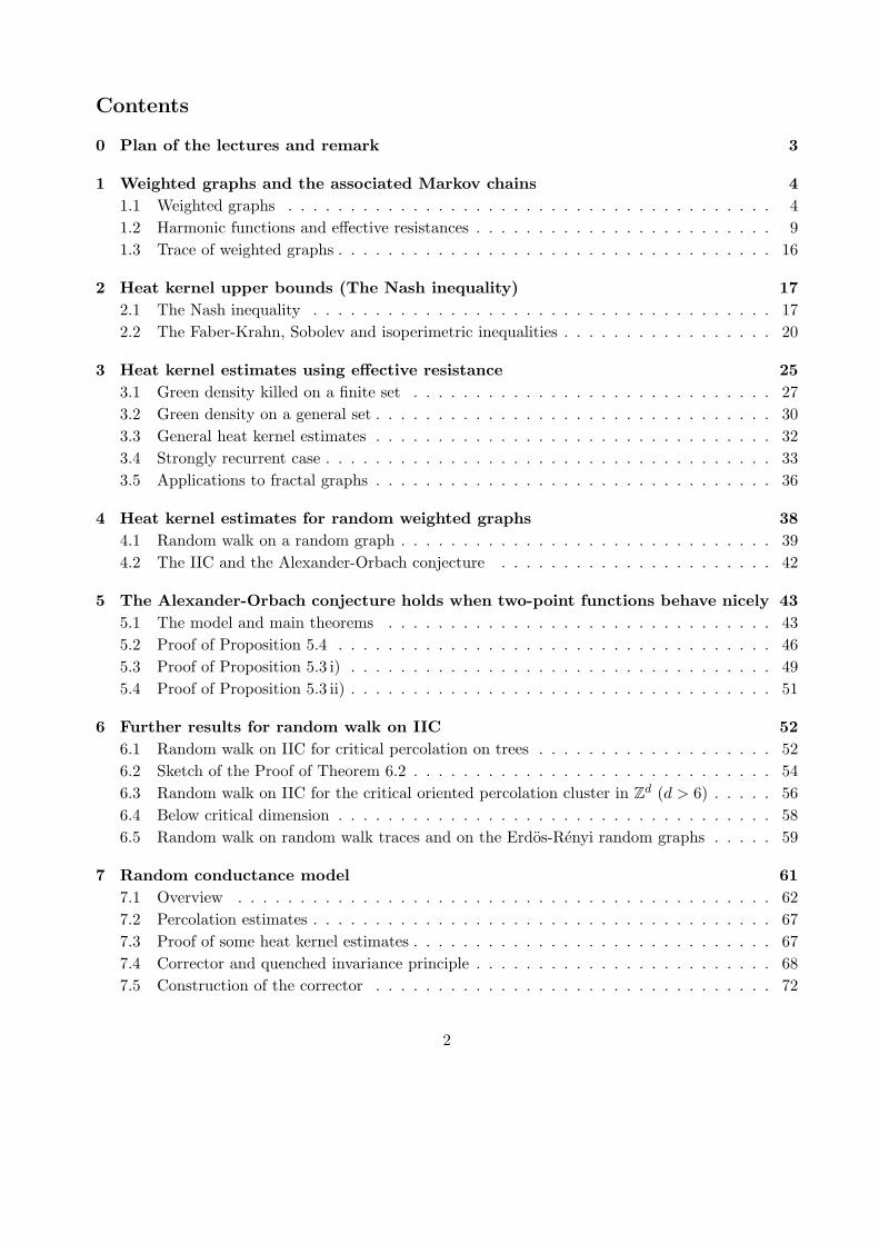
0
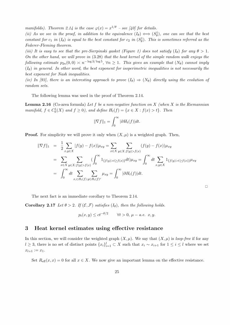
Figure 1: 2-dimensional pre-Sierpinski gasket
Remark 2.15 (i) Generalizations of (Sp✓ ) and (I✓) are the following:
kfkp c1'(µ(⌦))krfkp, 8⌦ ⇢⇢ X, 8f 2 F \ C0(X) such that Supp f ⇢ Cl(⌦),1
'(µ(⌦)) c2
|@⌦|µ(⌦)
, 8⌦ ⇢⇢ X,
where ' : (0,1) ! (0,1) is a non-decreasing function as in Remark 2.10. Note that we defined(Sp✓ ) for p = 1, 2, but the above generalization makes sense for all p 2 [1,1] (at least for Riemannian
24
manifolds). Theorem 2.14 is the case '(x) = x1/✓ – see [40] for details.(ii) As we see in the proof, in addition to the equivalence (I✓) () (S1
✓ ), one can see that the bestconstant for c1 in (I✓) is equal to the best constant for c2 in (S1
✓ ). This is sometimes referred as theFederer-Fleming theorem.(iii) It is easy to see that the pre-Sierpinski gasket (Figure 1) does not satisfy (I✓) for any ✓ > 1.On the other hand, we will prove in (3.28) that the heat kernel of the simple random walk enjoys thefollowing estimate p2n(0, 0) ⇣ n� log 3/ log 5, 8n � 1. This gives an example that (N✓) cannot imply(I✓) in general. In other word, the best exponent for isoperimetric inequalities is not necessarily thebest exponent for Nash inequalities.(iv) In [93], there is an interesting approach to prove (I✓) ) (N✓) directly using the evolution ofrandom sets.
The following lemma was used in the proof of Theorem 2.14.
Lemma 2.16 (Co-area formula) Let f be a non-negative function on X (when X is the Riemannianmanifold, f 2 C1
0 (X) and f � 0), and define Ht(f) = {x 2 X : f(x) > t}. Then
krfk1 =Z 1
0|@Ht(f)|dt.
Proof. For simplicity we will prove it only when (X,µ) is a weighted graph. Then,
krfk1 =12
Xx,y2X
|f(y)� f(x)|µxy =Xx2X
Xy2X:f(y)>f(x)
(f(y)� f(x))µxy
=Xx2X
Xy2X:f(y)>f(x)
(Z 1
01{f(y)>t�f(x)}dt)µxy =
Z 1
0dt
Xx,y2X
1{f(y)>t�f(x)}µxy
=Z 1
0dt
Xx,2Ht(f)
Xy2Ht(f)c
µxy =Z 1
0|@Ht(f)|dt.
The next fact is an immediate corollary to Theorem 2.14.
Corollary 2.17 Let ✓ > 2. If (E ,F) satisfies (I✓), then the following holds.
pt(x, y) ct�✓/2 8t > 0, µ� a.e. x, y.
3 Heat kernel estimates using e↵ective resistance
In this section, we will consider the weighted graph (X,µ). We say that (X,µ) is loop-free if for anyl � 3, there is no set of distinct points {xi}l
i=1 ⇢ X such that xi ⇠ xi+1 for 1 i l where we setxl+1 := x1.
Set Re↵(x, x) = 0 for all x 2 X. We now give an important lemma on the e↵ective resistance.
25

Lemma 3.1 (i) If c1 := infx,y2X:x⇠y µxy > 0 then Re↵(x, y) c�11 d(x, y) for all x, y 2 X.
(ii) If (X,µ) is loop-free and c2 := supx,y2X:x⇠y µxy < 1, then Re↵(x, y) � c�12 d(x, y) for all
x, y 2 X.(iii) |f(x)� f(y)|2 Re↵(x, y)E(f, f) for all x, y 2 X and f 2 H2.(iv) Re↵(·, ·) and Re↵(·, ·)1/2 are both metrics on X.
Proof. (i) Take a shortest path between x and y and cut all the bonds that are not along the path.Then we have the inequality by the cutting law.(ii) Suppose d(x, y) = n. Take a shortest path (x0, x1, · · · , xn) between x and y so that x0 = x, xn =y. Now take f : X ! R so that f(xi) = (n � i)/n for 0 i n, and f(y) = f(xi) if y is in thebranch from xi, i.e. if y can be connected to xi without crossing {xk}n
k=0\{xi}. This f is well-definedbecause (X,µ) is loop-free, and f(x) = 1, f(y) = 0. So Re↵(x, y)�1
Pn�1i=0 (1/n)2µxixi+1 c2/n =
c2/d(x, y), and the result follows.(iii) For any non-constant function u 2 H2 and any x 6= y 2 X, we can construct f 2 H2 such thatf(x) = 1, f(y) = 0 by a linear transform f(z) = au(z) + b (where a, b are chosen suitably). So
supn |u(x)� u(y)|2
E(u, u): u 2 H2, E(u, u) > 0
o= sup
n 1E(f, f)
: f 2 H2, f(x) = 1, f(y) = 0o
= Re↵(x, y),
(3.1)and we have the desired inequality.(iv) It is easy to see Re↵(x, y) = Re↵(y, x) and Re↵(x, y) = 0 if and only if x = y. So we only needto check the triangle inequality.
Let H2 = {u 2 H2 : E(u, u) > 0}. Then, for x, y, z 2 X that are distinct, we have by (3.1)
Re↵(x, y)1/2 = supn |u(x)� u(y)|
E(u, u)1/2: u 2 H2
o
supn |u(x)� u(z)|
E(u, u)1/2: u 2 H2
o+ sup
n |u(z)� u(y)|E(u, u)1/2
: u 2 H2o
= Re↵(x, z)1/2 + Re↵(z, y)1/2.
So Re↵(·, ·)1/2 is a metric on X.Next, let V = {x, y, z} ⇢ X and let {µxy, µyz, µzx} be the trace of {µxy}x,y2X to V . Define
R�1xy = µxy, R�1
yz = µyz, R�1zx = µzx. Then, using Proposition 1.25 and the resistance formula of
series and parallel circuits, we have
Re↵(z, x) =1
R�1zx + (Rxy + Ryz)�1
=Rzx(Rxy + Ryz)Rxy + Ryz + Rzx
, (3.2)
and similarly Re↵(x, y) = Rxy(Ryz+Rzx)Rxy+Ryz+Rzx
and Re↵(y, z) = Ryz(Rzx+Rxy)Rxy+Ryz+Rzx
. Hence
12{Re↵(x, z) + Re↵(z, y)�Re↵(x, y)} =
RyzRzx
Rxy + Ryz + Rzx� 0, (3.3)
which shows that Re↵(·, ·) is a metric on X.
26

Remark 3.2 (i) Di↵erent proofs of the triangle inequality of Re↵(·, ·) in Lemma 3.1(iv) can be foundin [10] and [75, Theorem 1.12].(ii) Weighted graphs are resistance forms. (See [79] for definition and properties of the resistanceform.) In fact, most of the results in this section (including this lemma) hold for resistance forms.
3.1 Green density killed on a finite set
For y 2 X and n 2 N, let
L(y, n) =n�1Xk=0
1{Yk=y}
be the local time at y up to time n � 1. For a finite set B ⇢ X and x, y 2 X, define the Greendensity by
gB(x, y) =1µy
Ex[L(y,⌧B)] =1µy
Xk
Px(Yk = y, k <⌧ B). (3.4)
Clearly gB(x, y) = 0 when either x or y is outside B. Since µ�1y Px(Yk = y, k <⌧ B) = µ�1
x Py(Yk =x, k <⌧ B), we have
gB(x, y) = gB(y, x) 8x, y 2 X. (3.5)
Using the strong Markov property of Y ,
gB(x, y) = Px(�y < ⌧B)gB(y, y) gB(y, y). (3.6)
Below are further properties of the Green density.
Lemma 3.3 Let B ⇢ X be a finite set. Then the following hold.(i) For x 2 B, gB(x, ·) is harmonic on B \ {x} and = 0 outside B.(ii) (Reproducing property of the Green density) For all f 2 H2 with Supp f ⇢ B, it holds thatE(gB(x, ·), f) = f(x) for each x 2 X.(iii) Ex[⌧B] =
Py2B gB(x, y)µy for each x 2 X.
(iv) Re↵(x,Bc) = gB(x, x) for each x 2 X.(v) Ex[⌧B] Re↵(x, Bc)µ(B) for each x 2 X.
Proof. (i) Let ⌫(z) = gB(x, z). Then, for each y 2 B \ {x}, noting that Y0, Y⌧B /2 B, we have
⌫(y)µy = Ex[⌧B�1Xi=0
1y(Yi+1)] = Ex[⌧B�1Xi=0
Xz
1z(Yi)P (z, y)] =X
z
⌫(z)µzµzy
µz=X
z
⌫(z)µyz
Dividing both sides by µy, we have ⌫(y) =P
z P (y, z)⌫(z), so ⌫ is harmonic on B \ {x}.(ii) Let u(y) = ⌫(y)µy. Since ⌫ is harmonic on B \ {x} and Supp f ⇢ B, noting that we can apply
27
Lemma 1.5 (ii) because f 2 L2 when B is finite, we have
E(⌫, f) = ��⌫(x)f(x)µx = {⌫(x)�X
y
P (x, y)⌫(y)}f(x)µx
= {⌫(x)µx �X
y
µxy
µxµx⌫(y)}f(x) = {⌫(x)µx �
Xy
µxy
µyµy⌫(y)}f(x)
= {u(x)�X
y
P (y, x)u(y)}f(x). (3.7)
Since u(y) = Ex[P⌧B�1
k=0 1{Yk=y}] andP
y 1{Yk=y}P (y, x) = 1{Yk+1=x}, we have
u(x)�X
y
P (y, x)u(y) = Exh ⌧B�1X
k=0
1{Yk=x}i� Ex
h ⌧B�1Xk=0
Xy
1{Yk=y}P (y, x)i
= 1 + Exh ⌧B�1X
k=1
1{Yk=x}i� Ex
h ⌧B�1Xk=0
1{Yk+1=x}i
= 1 + Exh ⌧B�1X
k=1
1{Yk=x}i� Ex
h ⌧BXk=1
1{Yk=x}i
= 1.
Putting this into (3.7), we obtain E(⌫, f) = f(x).(iii) Multiplying both sides of (3.4) by µy and summing over y 2 B, we obtain the result.(iv) If x /2 B, both sides are 0, so let x 2 B. Let px
B(z) = gB(x, z)/gB(x, x). Then, by Proposition1.13 and (i) above, we see that px
B attains the minimum in the definition of the e↵ective resistance.(Note that the assumption that B is finite is used to guarantee the uniqueness of the minimum.)Thus, using (ii) above,
Re↵(x, Bc)�1 = E(pxB, px
B) =E(gB(x, ·), gB(x, ·))
gB(x, x)2=
1gB(x, x)
. (3.8)
(v) If x /2 B, both sides are 0, so let x 2 B. Using (iii), (iv) and (3.6), we have
Ex[⌧B] =Xy2B
gB(x, y)µy Xy2B
gB(x, x)µy = Re↵(x,Bc)µ(B).
We thus obtain the desired inequality.
Remark 3.4 As mentioned before Definition 1.3, �(u(x)�P
y P (y, x)u(y)) in (3.7) is the total fluxflowing into x, given the potential ⌫. So, we see that the total flux flowing out from x is 1 when thepotential gB(x, ·) is given at x.
The next example shows that Re↵(x,Bc) = gB(x, x) does not hold in general when B is not finite.
Example 3.5 Consider Z3 with weight 1 on each nearest neighbor bond. Let p be an additionalpoint and put a bond with weight 1 between the origin of Z3 and p; X = Z3 [ {p} with the above
28
mentioned weights is the weighted graph in this example. Let B = Z3 and let Bn = B \B(0, n). ByLemma 3.3(iv), Re↵(0, Bc
n) = gBn(0, 0). If we set c�1n := RZ3
e↵ (0, B(0, n)), then it is easy to computeRe↵(0, Bc
n) = (1 + cn)�1. Since the simple random walk on Z3 is transient, limn!1 cn =: c0 > 0.As will be proved in the proof of Lemma 3.9, gB(0, 0) = limn!1 gBn(0, 0), so gB(0, 0) = (1 + c0)�1.On the other hand, it is easy to see Re↵(0, Bc) = 1 > (1 + c0)�1, so Re↵(0, Bc) > gB(0, 0). Thisalso shows that in general the resistance between two sets cannot be approximated by the resistanceof finite approximation graphs.
For any A ⇢ X, and A1, A2 ⇢ X with A1 \A2 = ;, A \Ai = ; (for either i = 1 or 2) define
RAe↵(A1, A2)�1 = inf{E(f, f) : f 2 H2, f |A1 = 1, f |A2 = 0, f is a constant on A}.
In other word, RAe↵(·, ·) is the e↵ective resistance for the network where the set A is shorted and
reduced to one point. Clearly RAe↵(x, A) = Re↵(x,A) for x 2 X \A. We then have the following.
Proposition 3.6 Let B ⇢ X be a finite set. Then
gB(x, y) =12(Re↵(x, Bc) + Re↵(y,Bc)�RBc
e↵ (x, y)), 8x, y 2 B.
Proof. Since the set Bc is reduced to one point, it is enough to prove this when Bc is a point, sayz. Noting that R{z}
e↵ (x, y) = Re↵(x, y), we will prove the following.
gX\{z}(x, y) =12(Re↵(x, z) + Re↵(y, z)�Re↵(x, y)), 8x, y 2 B. (3.9)
By Lemma 3.3 (iv) and (3.6), we have
gX\{z}(x, y) = Py(�x < ⌧X\{z})gX\{z}(x, x) = Py(�x < �z)Re↵(x, z). (3.10)
Now V = {x, y, z} ⇢ X and consider the trace of the network to V , and consider the function u onV such that u(x) = 1, u(z) = 0 and u is harmonic on y. Using the same notation as in the proof ofLemma 3.1 (iv), we have
Py(�x < �z) = u(y) =R�1
xy
R�1xy + R�1
yz⇥ 1 +
R�1yz
R�1xy + R�1
yz⇥ 0 =
Ryz
Rxy + Ryz.
Putting this into (3.10) and using (3.2), we have
gB(x, y) =Ryz
Rxy + Ryz· Rzx(Rxy + Ryz)Rxy + Ryz + Rzx
=RzxRyz
Rxy + Ryz + Rzx. (3.11)
By (3.3), we obtain (3.9).
Remark 3.7 Take an additional point p0 and consider the �-Y transform between V = {x, y, z}and W = {p0, x, y, z}. Namely, W = {p0, x, y, z} is the network such that µp0x, µp0y, µp0z > 0 andother weights are 0, and the trace of (W, µ) to V is (V, µ). (See, for example, [79, Lemma 2.1.15].)Then RzxRyz
Rxy+Ryz+Rzxin (3.11) is equal to µ�1
p0z, so gB(x, y) = µ�1p0z.
29

Corollary 3.8 Let B ⇢ X be a finite set. Then
|gB(x, y)� gB(x, z)| Re↵(y, z), 8x, y, z 2 X.
Proof. By Proposition 3.6, we have
|gB(x, y)� gB(x, z)| |Re↵(y,Bc)�Re↵(z,Bc)|+ |RBc
e↵ (x, y)�RBc
e↵ (x, z)|2
Re↵(y, z) + RBc
e↵ (y, z)2
Re↵(y, z),
which gives the desired result.
3.2 Green density on a general set
In this subsection, will discuss the Green density when B can be infinite. Since we do not use resultsin this subsection later, readers may skip this subsection.
Let B ⇢ X. We define the Green density by (3.4). By Proposition 1.18, gB(x, y) < 1 for allx, y 2 X when {Yn} is transient, whereas gX(x, y) = 1 for all x, y 2 X when {Yn} is recurrent. Sincethere is nothing interesting when gX(x, y) = 1, throughout this subsection we will only consider thecase
B 6= X when {Yn} is recurrent.
Then we can easily see that the process {Y Bn } killed on exiting B is transient, so gB(x, y) < 1 for
all x, y 2 X. It is easy to see that (3.5), (3.6), and Lemma 3.3 (i), (iii) hold without any change ofthe proof.
Recall that H20 is the closure of C0(X) in H2. We can generalize Lemma 3.3 (ii) as follows.
Lemma 3.9 (Reproducing property of Green density) For each x 2 X, gB(x, ·) 2 H20 . Further, for
all f 2 H20 with Supp f ⇢ B, it holds that E(gB(x, ·), f) = f(x) for each x 2 X.
Proof. When B is finite, this is already proved in Lemma 3.3 (ii), so let B be finite (and B 6= X
if {Yn} is recurrent). Fix x0 2 X and let Bn = B(x0, n) \ B and write ⌫n(z) = gBn(x, z). Then⌧Bn " ⌧B so that ⌫n(z) " ⌫(z) < 1 for all z 2 X. Using the reproducing property, for m n, wehave
E(⌫n � ⌫m, ⌫n � ⌫m) = gBn(x, x)� gBm(x, x),
which implies that {⌫n} is the Cauchy sequence in H2. It follows that ⌫n ! ⌫ in H2 and ⌫ 2 H20 .
Now for each f 2 H20 with Supp f ⇢ B, choose fn 2 C0(X) so that Supp f ⇢ Bn and fn ! f in H2.
Then, as we proved above, E(fn, ⌫n) = fn(x). Taking n ! 1 and using Lemma 1.2 (i), we obtainE(f,⌫ ) = f(x).
As we see in Example 3.5, Re↵(0, Bc) = limn!1Re↵(0, (B \ B(0, n)c) does not hold in general.So we introduce another resistance metric as follows.
R⇤(x, y) := supn |u(x)� u(y)|2
E(u, u): u 2 H2
0 � 1, E(u, u) > 0o
, 8x, y 2 X,x 6= y,
30

where H20 � 1 = {f + a : f 2 H2
0 , a 2 R}. By (3.1), the di↵erence between this and the e↵ectiveresistance metric is that either supremum is taken over all H2
0 � 1 or over all H2. Clearly R⇤(x, y) Re↵(x, y).
Here and in the following of this subsection, we will consider R⇤(x,Bc), so we assume B 6= X.(For R⇤(x,Bc), we consider Bc as one point by shorting.) Using R⇤(·, ·), we can generalize Lemma3.3 (iv),(v) as follows.
Lemma 3.10 Let B ⇢ X be a set such that B 6= X. Then the following hold.(i) R⇤(x,Bc) = gB(x, x) for each x 2 X.(ii) Ex[⌧B] R⇤(x, Bc)µ(B) for each x 2 X.
Proof. (i) If x /2 B, both sides are 0, so let x 2 B. Let pxB(z) = gB(x, z)/gB(x, x). Note that we
cannot follow the proof Lemma 3.3 (iv) directly because we do not have uniqueness for the solutionof the Dirichlet problem in general. Instead, we discuss as follows. Rewriting the definition, we have
R⇤(x,Bc)�1 = inf{E(f, f) : f 2 H20,x(B)} where H2
0,x(B) := {f 2 H20 � 1 : Supp f ⇢ B, f(x) = 1}.
(3.12)Take any v 2 H2
0,x(B). (Note that H20,x(B) ⇢ H2
0 since B 6= X.) Then, by Lemma 3.9,
E(v � pxB, px
B) =E(v � px
B, gB(x, ·))gB(x, x)
=v(x)� px
B(x)gB(x, x)
= 0.
So we haveE(v, v) = E(v � px
B, v � pxB) + E(px
B, pxB) � E(px
B, pxB),
which shows that the infimum in (3.12) is attained by pxB. Thus by (3.8) with R⇤(·, ·) instead of
Re↵(·, ·), we obtain (i).Given (i), (ii) can be proved exactly in the same way as the proof of Lemma 3.3 (v).
Remark 3.11 As mentioned in [78, Section 2], when (X,µ) is transient, one can show that (E , H20�
1) is the resistance form on X [ {�}, where {�} is a new point that can be regarded as a point ofinfinity. Note that there is no weighted graph (X [ {�}, µ) whose associated resistance form is(E , H2
0 � 1). Indeed, if there is, then 1{�} 2 H20 � 1, which contradicts the fact 1 /2 H2
0 (Proposition1.22).
Given Lemma 3.10, Proposition 3.6 and Corollary 3.8 holds in general by changing Re↵(·, ·) toR⇤(·, ·) without any change of the proof.
Finally, note that by Proposition 1.24, we see that H2 = H20 � 1 if and only if there is no non-
constant harmonic functions of finite energy. One can see that it is also equivalent to Re↵(x, y) =R⇤(x, y) for all x, y 2 X. (The necessity can be shown by the fact that the resistance metricdetermines the resistance form: see [79, Section 2.3].)
31

3.3 General heat kernel estimates
In this subsection, we give general on-diagonal upper and lower heat kernel estimates. Define
B(x, r) = {y 2 X : d(x, y) < r}, V (x,R) = µ(B(x,R)).
For⌦ ⇢ X, let r(⌦) be the inradius, that is
r(⌦) = max{r 2 N : 9x0 2 ⌦ such that B(x0, r) ⇢ ⌦}.
Lemma 3.12 Assume that infx,y2X:x⇠y µxy > 0.(i) For any non-void finite set ⌦ ⇢ X,
�1(⌦) � c1
r(⌦)µ(⌦). (3.13)
(ii) Suppose that there exists a strictly increasing function v on N such that
V (x, r) � v(r), 8x 2 X,8r 2 N. (3.14)
Then, for any non-void finite set ⌦ ⇢ X,
�1(⌦) � c1
v�1(µ(⌦))µ(⌦). (3.15)
Proof. (i) Let f be any function with Supp f ⇢ ⌦ normalized as kfk1 = 1. Then kfk22 µ(⌦).Now consider a point x0 2 X such that |f(x0)| = 1 and the largest integer n such that B(x0, n) ⇢ ⌦.Then n r(⌦) and there exists a sequence {xi}n
i=0 ⇢ X such that xi ⇠ xi+1 for i = 0, 1, · · · , n� 1,xj 2 ⌦ for j = 0, 1, · · · , n� 1 and xn /2 ⌦. So we have
E(f, f) � 12
n�1Xi=0
(f(xi)� f(xi+1))2µxixi+1 �c1
n
⇣ n�1Xi=0
|f(xi)� f(xi+1)|⌘2� c1
n,
where the last inequality is due toPn�1
i=0 |f(xi)� f(xi+1)| � |f(x0)� f(xn)| = 1. Combining these,
E(f, f)kfk22
� c1
nµ(⌦)� c1
r(⌦)µ(⌦).
Taking infimum over all such f , we obtain the result.(ii) Denote r = r(⌦). Then, there exists x0 2 ⌦ such that B(x0, r) ⇢ ⌦, so (3.14) implies v(r) µ(⌦).Thus r v�1(µ(⌦)), and (3.15) follows from (3.13).
Proposition 3.13 (Upper bound: slow decay) Assume that infx,y2X:x⇠y µxy > 0 and
V (x, r) � c1rD, 8x 2 X,8r 2 N, (3.16)
for some D � 1. Then the following holds.
supx2X
pt(x, x) c2t� D
D+1 , 8t � 1.
32

Proof. By (3.15), we have �1(⌦) � c1µ(⌦)�1�1/D. Thus the result is obtained by Theorem 2.14 bytaking ✓ = 2D/(D + 1).
Remark 3.14 We can generalize Proposition 3.13 as follows (see [14]):Assume that infx,y2X:x⇠y µxy > 0 and (3.14) holds for all r � r0. Then the following holds.
supx2X
pt(x, x) c1m(t), 8t � r20,
where m is defined by
t� r20 =
Z 1/m(t)
v(r0)v�1(s)ds.
Indeed, by (3.14), we see that (2.6) holds with '(s)2 = cv�1(s)s. Thus the result can be obtainedby applying Remark 2.5 and Remark 2.10. In fact, the above generalized version of Proposition 3.13also holds for geodetically complete non-compact Riemannian manifolds with bounded geometry (see[14]).
Below is the table of the slow heat kernel decay m(t), given the information of the volume growthv(r).
V (x, r) � exp(cr) c exp(cr↵) crD cr
supx2X pt(x, x) ct�1 log t ct�1(log t)1/↵ ct�D/(D+1) ct�1/2
Next we discuss general form of the on-diagonal heat kernel estimate. This lower bound is quiterobust, and the argument works as long as there is a Hunt process and the heat kernel exists. Notethat the estimate is independent of the upper bound, so in general the two estimates may not coincide.
Proposition 3.15 (Lower bound) Let B ⇢ X and x 2 B. Then
p2t(x, x) � Px(⌧B > t)2
µ(B), 8t > 0.
Proof. Using the Chapman-Kolmogorov equation and the Schwarz inequality, we have
Px(⌧B > t)2 Px(Yt 2 B)2 = (Z
Bpt(x, y)dµ(y))2 µ(B)
ZB
pt(x, y)2dµ(y) µ(B)p2t(x, x),
which gives the desired inequality.
3.4 Strongly recurrent case
In this subsection, we will restrict ourselves to the ‘strongly recurrent’ case and give su�cient condi-tions for precise on-diagonal upper and lower estimates of the heat kernel. (To be precise, Proposition3.16 holds for general weighted graphs, but the assumption FR,� given in other propositions holdsonly for the strongly recurrent case.)
33

Throughout this subsection, we fix a based point 0 2 X and let D � 1, 0 < ↵ 1. As befored(·, ·) is a graph distance, but we do not use the property of the graph distance except in Remark3.17. In fact all the results in this subsection hold for any metric (not necessarily a geodesic metric)on X without any change of the proof.
Proposition 3.16 For n 2 N, let fn(x) = pn(0, x) + pn+1(0, x). Assume that Re↵(0, y) c⇤d(0, y)↵
holds for all y 2 X. Let r 2 N and n = 2[r]D+↵. Then
fn(0) c1n� D
D+↵
⇣c⇤ _
rD
V (0, r)
⌘. (3.17)
Especially, if c2rD V (0, r), then fn(0) c3n�D/(D+↵).
Proof. First, note that similarly to (1.7), we can easily check that
E(fn, fn) = f2n(0)� f2n+2(0). (3.18)
Choose x⇤ 2 B(0, r) such that fn(x⇤) = minx2B(0,r) fn(x). Then
fn(x⇤)V (0, r) X
x2B(0,r)
fn(x)µx Xx2G
pn(0, x)µx +Xx2G
pn+1(0, x)µx 2,
so that fn(x⇤) 2/V (0, r). Using Lemma 3.1 (iii), Re↵(0, y) c⇤d(0, y)↵, and (3.18), we have
fn(0)2 2�fn(x⇤)2 + |fn(0)� fn(x⇤)|2
� 8
V (0, r)2+ 2Re↵(0, x⇤)E(fn, fn)
8V (0, r)2
+ 2c⇤d(0, x⇤)↵E(fn, fn) 8V (0, r)2
+ 2c⇤d(0, x⇤)↵(f2n(0)� f2n+2(0)). (3.19)
The spectral decomposition gives that k ! f2k(0)� f2k+2(0) is non-increasing. Thus
n (f2n(0)� f2n+2(0)) (2[n/2] + 1)�f4[n/2](0)� f4[n/2]+2(0)
�
22[n/2]Xi=[n/2]
(f2i(0)� f2i+2(0)) 2f2[n/2](0).
Since n = 2[r]D+↵ is even, putting this into (3.19), we have fn(0)2 8V (0,r)2 + 4c⇤r↵fn(0)
n . Usinga + b 2(a _ b), we have
fn(0) c1(1
V (0, r)_ c⇤r↵
n). (3.20)
Rewriting, we obtain (3.17).
Remark 3.17 (i) Putting n = 2[r↵V (0, r)] in (3.20), we have the following estimate:
f2[r↵V (0,r)](0) c1(1 _ c⇤)V (0, r)
. (3.21)
(ii) When ↵ = 1, using Lemma 3.1(i), we see that the assumption of Proposition 3.16 holds ifinfx,y2X:x⇠y µxy > 0. So (3.17) gives another proof of Proposition 3.13.
34
In the following, we write BR = B(0, R). Let "� = (3c⇤�)�1/↵. We say the weighted graph (X,µ)satisfies FR,� (or simply say that FR,� holds) if it satisfies the following estimates:
V (0, R) �RD, Re↵(0, z) c⇤d(0, z)↵, 8z 2 BR, Re↵(0, BcR) � R↵
�, V (0, "�R) � ("�R)D
�. (3.22)
Proposition 3.18 In the following, we fix R � 1 and � > 0.(i) If V (0, R) �RD, Re↵(0, z) c⇤d(0, z)↵ for all z 2 BR, then the following holds.
Ex[⌧BR ] 2c⇤�RD+↵ 8x 2 BR. (3.23)
(ii) If FR,� holds, then there exist c1 = c1(c⇤), q0 > 0 such that the following holds for all x 2B(0, "�R).
Ex[⌧BR ] � c1��q0RD+↵, (3.24)
P x(⌧BR > n) � c1��q0RD+↵ � n
2c⇤�RD+↵8n � 0. (3.25)
Proof. (i) Using Lemma 3.3 (v) and the assumption, we have
Ex[⌧BR ] Re↵(x, BcR)µ(BR) (Re↵(0, x) + Re↵(0, Bc
R))µ(BR) 2c⇤�RD+↵, 8x 2 BR. (3.26)
(ii) Denote B0 = B(0, "�R). By Lemma 1.15 and the assumption, we have for y 2 B0,
Py(⌧BR < �{0}) = Py(�BcR
< �{0}) Re↵(y,Bc
R [ {0})Re↵(y,Bc
R) Re↵(y, 0)
Re↵(0, BcR)�Re↵(0, y)
c⇤d(y, 0)↵
Re↵(0, BcR)� c⇤d(y, 0)↵
R↵/(3�)R↵/��R↵/(3�)
=12.
Applying this into (3.6) and using Lemma 3.3 (v), we have for y 2 B0,
gBR(0, y) = gBR(0, 0)Py(�{0} < ⌧BR) � 12Re↵(0, Bc
R) � R↵
2�.
Thus,
E0[⌧BR ] �Xy2B0
gB(0, y)µy �R↵
2�µ(B0) � "D� RD+↵
2�2.
Further, for x 2 B0,
Ex[⌧BR ] � Px(�{0} < �BR)E0[⌧BR ] � 12
E0[⌧BR ] � "D� RD+↵
4�2,
so (3.24) is obtained.Next, by (3.23), (3.24), and the Markov property of Y , we have
c1��q0RD+↵ Ex[⌧BR ] n + Ex[1{⌧BR
>n}EYn [⌧BR ]] n + 2c⇤�RD+↵Px(⌧BR > n).
So (3.25) is obtained.
35

Proposition 3.19 If FR,� holds, then there exist c1 = c1(c⇤), q0, q1 > 0 such that the following holdsfor all x 2 B(0, "�R).
p2n(x, x) � c1��q1n�D/(D+↵) for
c3.18.1
4�q0RD+↵ n c3.18.1
2�q0RD+↵.
Proof. Using Proposition 3.15 and (3.25), we have
p2n(x, x) � Px(⌧BR > n)2
µ(BR)� (c3.18.1/(2c⇤�q0+1))2
�RD� c1�
�q1n�D/(D+↵),
for some c1, q1 > 0.
Remark 3.20 The above results can be generalized as follows. Let v, r : N ! [0,1) be strictlyincreasing functions with v(1) = r(1) = 1 which satisfy
C�11
⇣ R
R0
⌘d1
v(R)v(R0)
C1
⇣ R
R0
⌘d2
, C�12
⇣ R
R0
⌘↵1
r(R)r(R0)
C2
⇣ R
R0
⌘↵2
for all 1 R0 R < 1, where C1, C2 � 1, 1 d1 d2 and 0 < ↵1 ↵2 1. Assume that thefollowing holds instead of (3.22) for a suitably chosen "� > 0:
V (0, R) �v(R), Re↵(0, z) c⇤r(d(0, z)), 8z 2 BR, Re↵(0, BcR) � r(R)
�, V (0, "�R) � v("�R)
�.
x 2 B(0, "�R). Then, the following estimates hold.c1
�q1v(I(n)) p2n(x, x) c2
�q2v(I(n))for
c0
4�q0v(R)r(R) n c0
2�q0v(R)r(R),
where I(·) is the inverse function of (v · r)(·) (see [87] for details).
3.5 Applications to fractal graphs
In this subsection, we will apply the estimates obtained in the previous subsection to fractal graphs.
2-dimensional pre-Sierpinski gasketLet V0 be the vertices of the pre-Sierpinski gasket (Figure 1) and define V�n = 2nV0. Let
an = (2n, 0), bn = (2n�1, 2n�1p
3) be the vertices in V�n.
Lemma 3.21 It holds that Re↵(0, {an, bn}) = 12
⇣53
⌘n.
Proof. Let pn = P0(�{an,bn} < �+{0}). Let z = (3/2,
p3/2) and define q1 = Pz(�{a1,b1} < �+
{0}).Then, by the Markov property, p1 = 4�1(p1 + q1 + 1) and q1 = 2�1(p1 + 1). Solving them, we havep1 = 3/5. Next, for a simple random walk {Yk} on the pre-Sierpinski gasket, define the inducedrandom walk {Y (n)
k } on V�n as follows.
⌘0 = min{k � 0 : Yk 2 V�n}, ⌘i = min{k > ⌘i�1 : Yk 2 V�n \ Y⌘i�1}, Y (n)i = Y⌘i , for i 2 N.
36
Then it can be easily seen that {Y (n)k } is a simple random walk on V�n. Using this fact, we can
inductively show pn+1 = pn · p1 = pn · (3/5) = · · · = (3/5)n+1. We thus obtain the result by usingTheorem 1.14.
Let df = log 3/ log 2, dw = log 5/ log 2.
Proposition 3.22 The following hold for all R � 1.(i) c1Rdf V (0, R) c2Rdf .
(ii) Re↵(0, z) c3d(0, z)dw�df , 8z 2 X.
(iii) Re↵(0, B(0, R)c) � c4Rdw�df .
Proof. (i) Since there are 3n triangles with length 1 in B(0, 2n), we see that c13n V (0, 2n) c23n.Next, for each R, take n 2 N such that 2n�1 R < 2n. Then c13n�1 V (0, 2n�1) V (0, R) V (0, 2n) c23n. Since 3 = 2df , we have the desired estimate.(ii) We first prove the following:
c3(5/3)n Re↵(0, an) c4(5/3)n. (3.27)
Indeed, by the shorting law and Lemma 3.21, 2�1(5/3)n = Re↵(0, {an, bn}) Re↵(0, an). On theother hand, let '(1)
n and '(2)n be such that
E('(1)n ,'(1)
n ) = Re↵(0, an)�1 = Re↵(0, bn)�1 = E('(2)n ,'(2)
n ).
Then, by symmetry, '(1)n (bn) = '(2)
n (an) =: C. So
12
⇣53
⌘n= Re↵(0, {an, bn}) � E
⇣'(1)n + '(2)
n
1 + C,'(1)
n + '(2)n
1 + C
⌘�1
�n 2
(1 + C)2⇣E('(1)
n ,'(1)n ) + E('(2)
n ,'(2)n )
⌘o�1=
(1 + C)2
4Re↵(0, an).
We thus obtain (3.27). Now for each z 2 X, choose n � 0 such that 2n d(0, z) < 2n+1. We can thentake a sequence z = z0, z1, · · · , zn such that zi 2 V�i, d(zi, zi+1) 2i for i = 0, 1, · · · , n�1 (zi = zi+1
is allowed) and d(0, zn) = 2n. Similarly to (3.27), we can show that Re↵(zi, zi+1) c5(5/3)i. Thus,using the triangle inequality, we have
Re↵(0, z) n�1Xi=0
Re↵(zi, zi+1) + Re↵(0, zn) c5
⇣ n�1Xi=0
(5/3)i + (5/3)n⌘ c6(5/3)n c7d(0, z)dw�df .
So the desired estimate is obtained.(iii) For each R, take n 2 N such that 2n�1 R < 2n. Then, by the shorting law and Lemma 3.21,
Re↵(0, B(0, R)c) � Re↵(0, {an, bn}) =12
⇣53
⌘n=
122n(dw�df ) � c8R
dw�df ,
so we have the desired estimate.
37

By Proposition 3.16, 3.19, 3.22, we see that the following heat kernel estimate holds for simplerandom walk on the 2-dimensional Sierpinski gasket.
c1n�df /dw p2n(0, 0) c2n
�df /dw , 8n � 1. (3.28)
Vicsek sets
0
Figure 2: 2-dimensional Vicsek set
We next consider the Vicsek set (Figure 2). Noting that this graph is loop-free, we can apply Lemma3.1 (ii), and Lemma 3.1 (i) trivially holds. So by a similar proof we can obtain Proposition 3.22 withdf = log 5/ log 3 and dw = df + 1, so (3.28) holds. This shows that the estimate in Proposition 3.13is in general the best possible estimate when D = log 5/ log 3. By considering the generalization ofVicsek set in Rd, we can see that the same is true when D = log(1 + 2d)/ log 3 (which is a sequencethat goes to infinity as d ! 1). In fact it is proved in [14, Theorem 5.1] that the estimate inProposition 3.13 is in general the best possible estimate for any D � 1.
Remark 3.23 It is known that the following heat kernel estimate holds for simple random walk onthe pre-Sierpinski gasket, on Vicsek sets, and in general on the so-called nested fractal graphs (see[65, 72]):
c1n�df /dw exp
⇣�c2
⇣d(x, y)dw
n
⌘ 1dw�1
⌘ pn(x, y)+pn+1(x, y) c3n
�df /dw exp⇣�c4
⇣d(x, y)dw
n
⌘ 1dw�1
⌘,
for all x, y 2 X, n � d(x, y). (Note that pn(x, y) = 0 if n < d(x, y).)
4 Heat kernel estimates for random weighted graphs
From this section, we consider the situation where we have a random weighted graph {(X(!), µ!) :! 2 ⌦} on a probability space (⌦,F , P). We assume that, for each ! 2 ⌦, the graph X(!) is infinite,locally finite and connected, and contains a marked vertex 0 2 G. We denote balls in X(!) byB!(x, r), their volume by V!(x, r), and write
B(R) = B!(R) = B!(0, R), V (R) = V!(R) = V!(0, R).
38

We write Y = (Yn, n � 0, P x! , x 2 X(!)) for the Markov chain on X(!), and denote by p!n(x, y) its
transition density with respect to µ!. Let
⌧R = ⌧B(0,R) = min{n � 0 : Yn /2 B(0, R)}.
4.1 Random walk on a random graph
Recall that FR,� is defined in (3.22). We have the following quenched estimates.
Theorem 4.1 Let R0,�0 � 1. Assume that there exist p(�) � 0 with p(�) c1��q0 for someq0, c1 > 0 such that for each R � R0 and � � �0,
P({! : (X(!), µ!) satisfies FR,�}) � 1� p(�). (4.1)
Then there exist ↵1,↵2 > 0 and ⌦0 ⇢ ⌦ with P(⌦0) = 1 such that the following holds: For all ! 2 ⌦0
and x 2 X(!), there exist Nx(!), Rx(!) 2 N such that
(log n)�↵1n�D
D+↵ p!2n(x, x) (log n)↵1n�D
D+↵ , 8n � Nx(!), (4.2)
(log R)�↵2RD+↵ Ex!⌧R (log R)↵2RD+↵, 8R � Rx(!). (4.3)
Further, if (4.1) holds with p(�) exp(�c2�q0) for some q0, c2 > 0, then (4.2), (4.3) hold withlog log n instead of log n.
Proof. We will take⌦ 0 = ⌦1 \ ⌦2 where⌦ 1 and⌦ 2 are defined below.First we prove (4.2). Write w(n) = p!2n(0, 0). By Proposition 3.16 and 3.19, we have, taking
n = [c1(�)RD+↵],P((c1�
q1)�1 nD/(D+↵)w(n) c1�q1) � 1� 2p(�). (4.4)
Let nk = [ek] and �k = k2/q0 (by choosing R suitably). Then, sinceP
p(�k) < 1, by the Borel–Cantelli lemma there exists K0(!) with P(K0 < 1) = 1 such that c�1
1 k�2q1/q0 nD/(D+↵)k w(nk)
c1k2q1/q0 for all k � K0(!). Let⌦ 1 = {K0 < 1}. For k � K0 we therefore have
c�12 (log nk)�2q1/q0n�D/(D+↵)
k w(nk) c2(log nk)2q1/q0n�D/(D+↵)k ,
so that (4.2) holds for the subsequence nk. The spectral decomposition gives that p!2n(0, 0) is mono-tone decreasing in n. So, if n > N0 = eK0 + 1, let k � K0 be such that nk n < nk+1. Then
w(n) w(nk) c2(log nk)2q1/q0n�D/(D+↵)k 2eD/(D+↵)c2(log n)2q1/q0n�D/(D+↵).
Similarly w(n) � w(nk+1) � c3n�D/(D+↵)(log n)�2q1/q0 . Taking q2 > 2q1/q0, so that the constantsc2, c3 can be absorbed into the log n term, we obtain (4.2) for x = 0.
If x, y 2 X(!) and k = d!(x, y), then using the Chapman–Kolmogorov equation
p!2n(x, x)(p!k (x, y)µx(!))2 p!2n+2k(y, y).
39

Let ! 2 ⌦1, x 2 X(!), write k = d!(0, x), h!(0, x) = (p!k (x, 0)µx(!))�2, and let n � N0(!) + 2k.Then
p!2n(x, x) h!(0, x)p!2n+2k(0, 0) h!(0, x)(log(n + k))q2
(n + k)D/(D+↵) h!(0, x)
(log(2n))q2
nD/(D+↵) (log n)1+q2
nD/(D+↵)
provided log n � 2q2h!(0, x). Taking
Nx(!) = exp(2q2h!(0, x)) + 2d!(0, x) + N0(!), (4.5)
and ↵1 = 1 + q2, this gives the upper bound in (4.2). The lower bound is obtained in the same way.
Next we prove (4.3). Write F (R) = Ex!⌧R. By (3.23) and (3.24), we have
P(c1��q0RD+↵ F (R) 2c2�RD+↵, 8x 2 B(0, "�R)) � 1� p(�). (4.6)
Let Rn = en and �n = n2/q0 , and let Fn be the event of the left hand side of (4.6) when R = Rn,� = �n. Then we have P(F c
n) p(�n) n�2, so by Borel–Cantelli, if⌦ 2 = lim inf Fn, then P(⌦2) = 1.Hence there exist M0 with M0(!) < 1 on⌦ 2, and c3, q3 > 0 such that for ! 2 ⌦2 and x 2 X(!),
(c3�q3n )�1 F (Rn)
RD+↵n
c3�q3n , (4.7)
provided n � M0(!) and n is also large enough so that x 2 B("�nRn). Writing Mx(!) for thesmallest such n,
c�13 (log Rn)�2q3/q0RD+↵
n F (Rn) c3(log Rn)2q3/q0RD+↵n , for all n � Mx(!).
As F (R) is monotone increasing, the same argument as in the proof of (4.2) above enables us toreplace F (Rn) by F (R), for all R � Rx = 1 + eMx . Taking ↵2 > 2q3/q0, we obtain (4.3).
The case p(�) exp(�c2�q0) can be proved similarly by the following changes; take �k =(e+(2/c2) log k)1/q0 instead of �k = k2/q0 , and take Nx(!) = exp(exp(Ch!(0, x)))+2d!(0, x)+N0(!)in (4.5). Then, log n (resp. log nk, log Rn) in the above proof are changed to log log n (resp. log log nk,log log Rn) and the proof goes through.
We also have the following annealed estimates. Note that there are no log terms in them.
Proposition 4.2 Suppose (4.1) holds for some p(�) � 0 which goes to 0 as � ! 1, and supposethe following hold,
E[Re↵(0, B(R)c)V (R)] c1RD+↵, 8R � 1. (4.8)
Then
c2RD+↵ E[E0
!⌧R] c3RD+↵, 8R � 1, (4.9)
c4n�D/(D+↵) E[p!2n(0, 0)], 8n � 1. (4.10)
40

Suppose in addition that there exist c5 > 0,�0 > 1 and q00 > 2 such that
P(��1RD V (R), Re↵(0, y) �d(0, y)↵, 8y 2 B(R)) � 1� c5
�q00, (4.11)
for each R � 1,� � �0. Then
E[p!2n(0, 0)] c6n�D/(D+↵), 8n � 1. (4.12)
Proof. We begin with the upper bounds in (4.9). By (3.26) and (4.8),
E[E0!⌧R] E[Re↵(0, B(R)c)V (R)] c1R
D+↵.
For the lower bounds, it is su�cient to find a set F ⇢ ⌦ of ‘good’ graphs with P(F ) � c2 > 0such that, for all ! 2 F we have suitable lower bounds on E0
!⌧R or p!2n(0, 0). We assume that R � 1is large enough so that "�0R � 1, where �0 is chosen large enough so that p(�0) < 1/4. We can thenobtain the results for all n (chosen below to depend on R) and R by adjusting the constants c2, c4
in (4.9) and (4.10).Let F be the event of the left hand side of (4.6) when � = �0. Then P(F ) � 3
4 , and for ! 2 F ,E0!⌧R � c3�
�q00 RD+↵. So,
E[E0· ⌧R] � E[E0
· ⌧R : F ] � c3��q00 RD+↵P(F ) � 3c3
4��q0
0 RD+↵.
Also, by (4.4), if n = [c4(�0)RD+↵], then p!2n(0, 0) � c5��q10 n�D/(D+↵). So, given n 2 N, choose R
so that n = [c4(�0)RD+↵] and let F be the event of the left hand side of (4.4). Then
Ep·2n(0, 0) � P(F )c5��q10 n�D/(D+↵) � 3c5
4��q1
0 n�D/(D+↵),
giving the lower bound in (4.10).Finally we prove (4.12). Let Hk be the event of the left hand side of (4.11) with � = k. By
(3.17), we see that p!2n(0, 0) c6kn�D/(D+↵) if ! 2 Hk, where R is chosen to satisfy n = 2[R]D+↵.Since P([kHk) = 1, using (4.11), we have
Ep!2n(0, 0) X
k
c6(k + 1)n�D/(D+↵)P(Hk+1 \Hk) X
k
c6(k + 1)n�D/(D+↵)P(Hck)
c7n�D/(D+↵)
Xk
(k + 1)k�q00 < 1,
since q00 > 2. We thus obtain (4.12).
Remark 4.3 With some extra e↵orts, one can obtain quenched estimates of max0kn d(0, Yk) andµ(Wn) where Wn = {Y0, Y1, · · · , Yn} (range of the random walk), and annealed lower bound ofE0!d(0, Yn). See [87, (1.23), (1.28), (1.31)] and [18, (1.16), (1.20), (1.23)].
41

4.2 The IIC and the Alexander-Orbach conjecture
The problem of random walk on a percolation cluster — the ‘ant in the labyrinth’ [57] — has receivedmuch attention both in the physics and the mathematics literature. From the next section, we willconsider random walk on a percolation cluster, so X(!) will be a percolation cluster.
Let us first recall the bond percolation model on the lattice Zd: each bond is open with probabilityp 2 (0, 1), independently of all the others. Let C(x) be the open cluster containing x; then if✓(p) = Pp(|C(x)| = +1) it is well known (see [61]) that there exists pc = pc(d) such that ✓(p) = 0 ifp < pc and ✓(p) > 0 if p > pc.
If d = 2 or d � 19 (or d > 6 for spread-out models mentioned below) it is known (see for example[61, 106]) that ✓(pc) = 0, and it is conjectured that this holds for d � 2. At the critical probabilityp = pc, it is believed that in any box of side n there exist with high probability open clusters ofdiameter of order n. For large n the local properties of these large finite clusters can, in certaincircumstances, be captured by regarding them as subsets of an infinite cluster G, called the incipientinfinite cluster (IIC for short). This IIC G = G(!) is our random weighted graph X(!).
IIC was constructed when d = 2 in [76], by taking the limit as N ! 1 of the cluster C(0)conditioned to intersect the boundary of a box of side N with center at the origin. For large d aconstruction of the IIC in Zd is given in [69], using the lace expansion. It is believed that the resultsthere will hold for any d > 6. [69] also gives the existence and some properties of the IIC for all d > 6for spread-out models: these include the case when there is a bond between x and y with probabilitypL�d whenever y is in a cube side L with center x, and the parameter L is large enough. We writeGd for the IIC in Zd. It is believed that the global properties of Gd are the same for all d > dc, bothfor nearest neighbor and spread-out models. (Here dc is the critical dimension which is 6 for thepercolation model.) In [69] it is proved for spread-out models that Gd has one end – i.e. any twopaths from 0 to infinity intersect infinitely often. See [106] for a summary of the high-dimensionalresults.
Let Y = {Y !t }t�0 be the (continuous time) simple random walk on Gd = Gd(!), and q!t (x, y) be
its heat kernel. Define the spectral dimension of Gd by
ds(Gd) = �2 limt!1
log q!t (x, x)log t
,
(if this limit exists). Alexander and Orbach [7] conjectured that, for any d � 2, ds(Gd) = 4/3. Whileit is now thought that this is unlikely to be true for small d (see [71, Section 7.4]), the results on thegeometry of Gd for spread-out models in [69] are consistent with this holding for d above the criticaldimension.
Recently, it is proved that the Alexander-Orbach conjecture holds for random walk for the IICon a tree ([19]), on a high dimensional oriented percolation cluster ([18]), and on a high dimensionalpercolation cluster ([86]). In all cases, we apply Theorem 4.1, namely we verify (4.1) with D = 2,↵ =1 to prove the Alexander-Orbach conjecture. We will discuss details in the next two sections.
42

5 The Alexander-Orbach conjecture holds when two-point func-
tions behave nicely
This section is based on the paper by Kozma-Nachmias ([86]) with some simplification by [101].
5.1 The model and main theorems
We write x $ y if x is connected to y by an open path. We write xr$y if there is an open path of
length less than or equal to r that connects x and y.
Definition 5.1 Let (X,E) be a infinite graph.(i) A bijection map f : X ! X is called a graph automorphism for X if {f(u), f(v)} 2 E if and onlyif {u, v} 2 E. Denote the set of all the automorphisms of X by Aut(X)(ii) (X,E) is said to be transitive if for any u, v 2 X, there exists � 2 Aut(X) such that �(u) = v.(iii) For each x 2 X, define the stabilizer of x by
S(x) = {� 2 Aut(X) : �(x) = x}.
(iv) A transitive graph X is unimodular if for each x, y 2 X,
|{�(y) : � 2 S(x)}| = |{�(x) : � 2 S(y)}|.
One of the important property of the unimodular transitive graph is that it satisfies the followingX
x,y,z2Xd(0,z)=K
P(x$0 = z$y) =X
x,y,z2Xd(x,z)=K
P(0$x = z$y), (5.1)
for each K 2 N. This can be verified on Zd using the property of group translations, and it can beextended to unimodular transitive graphs using the mass transport technique (see for example, [102,(3.14)]).
Let (X,µ) be a unimodular transitive weighted graph that has controlled weights, with weight 1on each bond, i.e. µxy = 1 for x ⇠ y. In this section, allowing some abuse of notation, we denoteB(x, r) = {y 2 X : d(x, y) r} and set @A = {x 2 A : 9z 2 Ac such that z ⇠ x}.
We fix a root 0 2 X as before. (Note that since the graph is unimodular and transitive, theresults in this section is independent of the choice of 0 2 X.) Consider a bond percolation on X andlet pc = pc(X) be its critical probability, namely
Pp(There exists an open 1-cluster.) > 0 for p > pc(X),
Pp(There exists an open 1-cluster.) = 0 for p < pc(X).
In this section, we will consider the case p = pc and denote P := Ppc . Throughout this section, weassume that the following limit exists (independently on how d(0, x) !1).
PIIC(F ) = limd(0,x)!1
P(F |0 $ x) (5.2)
43

for any cylinder event F (i.e., an event that depends only on the status of a finite number of edges).We denote the realization of IIC by G(!). For the critical bond percolations on Zd, this is proved in[69] for d large using the lace expansion.
We consider the following two conditions. The first is the triangle condition by Aizenman-Newman ([3]), which indicates mean-field behavior of the model:
Xx,y2X
P(0 $ x)P(x $ y)P(y $ 0) < 1. (5.3)
Note that the value of the left hand side of (5.3) does not change if 0 is changed to any v 2 X becauseX is unimodular and transitive.
The second is the following condition for two-point functions: There exist c0, c1, c2 > 0 and adecreasing function : R+ ! R+ with (r) c0 (2r) for all r > 0 such that
c1 (d(0, x)) P(0 $ x) c2 (d(0, x)) 8x 2 X such that x, (5.4)
where d(·, ·) is the original graph distance on X. Because X is transitive, we have P(y $ z) = P(0 $x) when d(0, x) = d(y, z).
Since X is unimodular and transitive, we can deduce the following from the above mentionedtwo conditions.
Lemma 5.2 (i) (5.3) implies the following open triangle condition:
limK!1
supw:d(0,w)�K
Xx,y2X
P(0$x)P(x$y)P(y$w) = 0 . (5.5)
(ii) (5.5) implies the following estimates: There exist C1, C2, C3 > 0 such that
P�|C(0)| > n
� C1n
�1/2, 8n � 1, (5.6)
C2(pc � p)�1 E[|C(0)|] C3(pc � p)�1, 8p < pc. (5.7)
where C(0) is the connected component containing 0.
Proof. (i) This is proved in [83] (see [23, Lemma 2.1] for Zd).(ii) (5.5) implies (5.7) (see [3, Proposition 3.2] for Zd and [102, Page 291] for general unimodulartransitive graphs), and the following for h > 0 small (see [23, (1.13)] for Zd and [102, Page 292] forgeneral unimodular transitive graphs).
c1h1/2
1Xj=1
P(|C(0)| = j)(1� e�jh) c2h1/2.
Taking h = 1/n, we have P�|C(0)| > n
� C1n�1/2.
For the critical bond percolations on Zd, (5.4) with (x) = x2�d was obtained by Hara, van derHofstad and Slade [67] for the spread-out model and d > 6, and by Hara [66] for the nearest-neighbor
44

model with d � 19 using the lace expansion. (They obtained the right asymptotic behavior includingthe constant.) Given (5.4) with (x) = x2�d for d > 6, it is easy to check that (5.3) holds as well.
For each subgraph G of X, write Gp for the result of p-bond percolation. Define B(x, r;G) ={z : dGpc
(x, z) r} where dGpc(x, z) is the length of the shortest path between x and z in Gpc (it is
1 if there is no such path). Note that pc = pc(X). Now define
H(r;G) = {@B(0, r;G) 6= ;}, �(r) = supG⇢X
P(H(r;G)).
Note that
�(r) = supG⇢X
P({@B(v, r;G) 6= ;}), E[|B(0, r)|] = E[|B(v, r)|], 8v 2 X, (5.8)
since X is transitive. The following two propositions play a key role.
Proposition 5.3 Assume that the triangle condition (5.3) holds. Then there exists a constant C > 0such that the following hold for all r � 1.
i) E[|B(0, r)|] Cr, ii)�( r) C/r.
Proposition 5.4 Assume that (5.4) and i), ii) in Proposition 5.3 hold. Then (4.1) in Theorem 4.1holds for PIIC with p(�) = ��1/2, D = 2 and ↵ = 1.
Consider simple random walk on the IIC and let p!n(·, ·) be its heat kernel. Combining the abovetwo propositions with Theorem 4.1, we can derive the following theorem.
Theorem 5.5 Assume that (5.3) and (5.4) hold. Then there exist ↵1 > 0 and N0(!) 2 N withP(N0(!) < 1) = 1 such that
(log n)�↵1n�23 p!2n(0, 0) (log n)↵1n�
23 , 8n � N0(!), PIIC � a.e. !.
In particular, the Alexander-Orbach conjecture holds for the IIC.
By the above mentioned reason, for the critical bond percolations on Zd, the Alexander-Orbachconjecture holds for the IIC for the spread-out model with d > 6, and for the nearest-neighbor modelwith d � 19.
Remark 5.6 (i) In fact, the existence of the limit in (5.2) is not relevant in the arguments. Indeed,even if the limit does not exist, subsequential limits exist due to compactness, and the above resultshold for each limit. So the conclusions of Theorem 5.5 hold for any IIC measure (i.e. any subse-quential limit).(ii) The opposite inequalities of Theorem 5.3 (i.e. E[|B(0, r)|] � C 0r and �(r) � C 0/r for all r � 1)hold under weaker assumption. See Proposition 5.12.
In the following subsections, we prove Proposition 5.3 and 5.4.
45
5.2 Proof of Proposition 5.4
The proof splits into three lemmas.
Lemma 5.7 Assume that (5.4) and i) in Proposition 5.3 hold. Then there exists a constant C > 0such that for r � 1 and x 2 X with d(0, x) � 2r, we have
P(|B(0, r)| � �r2|0 $ x) C��1, 8� � 1. (5.9)
Proof. It is enough to prove the following for r � 1 and x 2 X with d(0, x) � 2r:
E[|B(0, r)| · 1{0$x}⇤ c1r
2 (d(0, x)). (5.10)
Indeed, we then have, using (5.4) and (5.10),
P(|B(0, r)| � �r2|0 $ x) E[|B(0, r)||0 $ x]�r2
=E[|B(0, r)| · 1{0$x}
⇤�r2P(0 $ x)
c1r2 (d(0, x))�r2c2 (d(0, x))
c3��1,
which gives (5.9). So we will prove (5.10).We have
E[|B(0, r)| · 1{0$x}⇤
=X
z
P(0 r$z , 0$x) Xz,y
P({0 r$y} � {y r$z} � {y$x})
Xz,y
P(0 r$y)P(y r$z)P(y$x). (5.11)
Here the first inequality is because, if {0 r$z, 0$x} occurs, then there must exist some y such that{0 r$y}, {y r$z} and {y$x} occur disjointly. The second inequality uses the BK inequality twice.
For d(0, y) r and d(0, x) � 2r, we have d(x, y) � d(0, x)� d(0, y) � d(0, x)/2, so that
P(y$x) c4 (d(x, y)) c4 (d(0, x)/2) c5 (d(0, x)).
Thus,
(RHS of (5.11)) c5 (d(0, x))Xz,y
P(0 r$y)P(y r$z) c5r (d(0, x))Xz,y
P(0 r$y) c5r2 (d(0, x)).
Here we use i) in Proposition 5.3 to sum, first over z (note that (5.8) is used here) and then over y
in the second and the third inequality. We thus obtain (5.10).
Lemma 5.8 Assume that (5.4) and ii) in Proposition 5.3 hold. Then there exists a constant C > 0such that for r � 1 and x 2 X with d(0, x) � 2r, we have
P(|B(0, r)| r2��1|0 $ x) C��1, 8� � 1. (5.12)
46
Proof. It is enough to prove the following for r � 1, " < 1 and x 2 X with d(0, x) � 2r:
P⇣|B(0, r)| "r2 , 0$x
⌘ c1" (d(0, x)). (5.13)
Indeed, we then have, using (5.4) and (5.13),
P(|B(0, r)| r2��1|0 $ x) =P(|B(0, r)| r2��1, 0 $ x)
P(0 $ x) c1��1 (d(0, x))
c2 (d(0, x)) c3�
�1,
which gives (5.12). So we will prove (5.13).If |B(0, r)| "r2, there must exist j 2 [r/2, r] such that |@B(0, j)| 2"r. We fix the smallest
such j. Now, if 0$x, there exists a vertex y 2 @B(0, j) which is connected to x by a path that doesnot use any of the vertices in B(0, j � 1). We say this “x$y o↵ B(0, j � 1)”. Let A be a subgraphof X such that P(B(0, j) = A) > 0. It is clear that, for any A and any y 2 @A, {y$x o↵ A \ @A} isindependent of {B(0, j) = A}. Thus,
P(0$x | B(0, j) = A) X
y2@A
P(y$x o↵ A \ @A | B(0, j) = A)
=X
y2@A
P(y$x o↵ A \ @A) X
y2@A
P(y$x) C|@A| (d(0, x)), (5.14)
where we used d(x, y) � d(0, x) � d(0, y) � d(0, x)/2 in the last inequality. By the definition of j
we have |@A| 2"r and summing over all A with P(B(0, j) = A) > 0 and @B(0, r/2) 6= ; (because0$x) gives
P(|B(0, r)| "r2, 0$x) C"r (d(0, x)) ·XA
P(B(0, j) = A).
Since the events {B(0, j) = A1} and {B(0, j) = A2} are disjoint for A1 6= A2, we haveXA
P(B(0, j) = A) = P(@B(0, r/2) 6= ;) c/r,
where ii) in Proposition 5.3 is used in the last inequality. We thus obtain (5.13).
Lemma 5.9 Assume that (5.4) and i), ii) in Proposition 5.3 hold. Then there exists a constantC > 0 such that for r � 1 and x 2 X with d(0, x) � 2r, we have
P(Re↵(0, @B(0, r)) r��1|0 $ x) C��1/2, 8� � 1. (5.15)
Proof of Proposition 5.4. Note that Re↵(0, z) d(0, z) holds for all z 2 B(0, R), and |B(0, R)| V (0, R) c1|B(0, R)| for all R � 1. By Lemma 5.7, 5.8 and 5.9, for each R � 1 and x 2 X withd(0, x) � 2R, we have
P({! : B(0, R) satisfies FR,�}|0 $ x) � 1� 3C��1/2 8� � 1.
Using (5.2), we obtain the desired estimate.
So, all we need is to prove Lemma 5.9. We first give definition of lane introduced in [95] (similarnotion was also given in [19]).
47
Definition 5.10 (i) An edge e between @B(0, j�1) and @B(0, j) is called a lane for r if there existsa path with initial edge e from @B(0, j � 1) to @B(0, r) that does not return to @B(0, j � 1).(ii) Let 0 < j < r and � � 1. We say that a level j has �-lanes for r if there exist at least � edgesbetween @B(0, j � 1) and @B(0, j) which are lanes for r.(iii) We say that 0 is �-lane rich for r if more than half of j 2 [r/4, r/2] have �-lanes for r.
Note that if 0 is not �-lane rich for r, then
Re↵(0, @B(0, r)) � r
8�. (5.16)
Indeed, since 0 is not �-lane rich, there exist j1, j2, · · · , jl 2 [r/4, r/2], l � r/8 that do not have�-lanes. For j 2 [r/4, r/2], let
Jj = {e : e is a lane for r that is between @B(0, j � 1) and @B(0, j)}. (5.17)
Then {Jjk}lk=1 are disjoint cut-sets separating 0 from @B(0, r). Since |Jjk | �, by the shorting law
we have Re↵(0, @B(0, r)) �Pl
k=1 |Jjk |�1 � l/� � r/(8�), so that (5.16) holds.
Proof of Lemma 5.9. It is enough to prove the following for r � 1, � > 1 and x 2 X withd(0, x) � 2r:
P⇣Re↵(0, @B(0, r)) ��1r , 0$x
⌘ c1�
�1/2 (d(0, x)). (5.18)
Indeed, we then have, using (5.4) and (5.18),
P(Re↵(0, @B(0, r)) r��1|0 $ x) =P(Re↵(0, @B(0, r)) r��1, 0 $ x)
P(0 $ x)
c1��1/2 (d(0, x))c2 (d(0, x))
c3��1/2,
which gives (5.15). So we will prove (5.18). The proof consists of two steps.
Step 1 We will prove the following; There exists a constant C > 0 such that for any r � 1, for anyevent E measurable with respect to B(0, r) and for any x 2 X with d(0, x) � 2r,
P(E \ {0$x}) Cp
rP(E) (d(0, x)). (5.19)
We first note that by (5.10), there exists some j 2 [r/2, r] such that
E⇥|@B(0, j)| · 1{0$x}
⇤ Cr (d(0, x)).
Using this and the Chebyshev inequality, for each M > 0 we have
P(E \ {0$x}) P(|@B(0, j)| > M, 0$x) + P(E \{| @B(0, j)| M, 0$x})
Cr (d(0, x))M
+ P(E \{| @B(0, j)| M, 0$x}).
48

For the second term, using (5.14) we have, for each A,
P({B(0, j) = A} \ {0$x}) C|@A| (d(0, x))P(B(0, j) = A).
Summing over all subgraphs A which satisfy E (measurability of E with respect to B(0, r) is usedhere) and |@A| M gives P(E \{| @B(0, j)| M, 0$x}) CM (d(0, x))P(E). Thus
P(E \ {0$x}) Cr (d(0, x))M
+ CM (d(0, x))P(E).
Taking M =p
r/P(E), we obtain (5.19).
Step 2 For j 2 [r/4, r/2], let us condition on B(0, j), take an edge e between @B(0, j�1) and @B(0, j),and denote the end vertex of e in @B(0, j) by ve. Let Gj be a graph that one gets by removing allthe edges with at least one vertex in B(0, j � 1). Then, {e is a lane for r} ⇢ {@B(ve, r/2;Gj) 6= ;}in the graph Gj . By the definition of � and ii) in Proposition 5.3 (note that (5.8) is used here), wehave
P(@B(ve, r/2;Gj) 6= ;|B(0, j)) �(r/2) C/r.
Recall the definition of Jj in (5.17). By the above argument, we obtain
E[|Jj | | B(0, j)] = P (X
ve2@B(0,j)
1{e is a lane for r}|B(0, j))
P (X
ve2@B(0,j)
1{@B(ve,r/2;Gj)6=;}|B(0, j)) C
r|@B(0, j)|.
This together with i) in Proposition 5.3 implies
E[r/2X
j=r/4
|Jj |] =r/2X
j=r/4
XA
E[|Jj |1{B(0,j)=A}]
C
r
r/2Xj=r/4
XA
|@A|P(B(0, j) = A) =C
r
r/2Xj=r/4
E[|@B(0, j)|] C
rE[|B(0, r)|] C 0.
So, P(0 is �-lane rich for r) C/(�r). Combining this with (5.16), we obtain
P⇣Re↵(0, @B(0, r)) ��1r
⌘ C
�r.
(Here Re↵(0, @B(0, r)) = 1 if @B(0, r) = ;.) This together with (5.19) in Step 1 implies (5.18).
5.3 Proof of Proposition 5.3 i)
The original proof of Proposition 5.3 i) by Kozma-Nachmias ([86]) (with some simplification in [82])used an induction scheme which is new and nice, but it requires several pages. Very recently (in fact,2 weeks before the deadline of the lecture notes), I learned a nice short proof by Sapozhnikov [101]which we will follow. The proof is also robust in the sense we do not need the graph to be transitive(nor unimodular).
49

Proposition 5.11 If there exists C1 > 0 such that Ep[|C(0)|] < C1(pc � p)�1 for all p < pc, thenthere exists C2 > 0 such that E[|B(0, r)|] C2r for all r � 1.
Proof. It is su�cient to prove for r � 2/pc. For p < pc, we will consider the coupling of percolationwith parameter p and pc as follows. First, each edge is open with probability pc and closed with1�pc independently. Then, for each open edge, the edge is kept open with probability p/pc and getsclosed with 1� p/pc independently. By the construction, for each r 2 N, we have
Pp(xr$y) �
⇣ p
pc
⌘rPpc(x
r$y), 8x, y 2 X.
Summing over y 2 X and using Pp(xr$y) Pp(x$y) and the assumption, we have
E[|B(0, r)|] ⇣ p
pc
⌘rEp[|C(0)|]
⇣ p
pc
⌘r(pc � p)�1.
Taking p = pc � 1/r, we obtain the result.
Using Lemma 5.2, we see that (5.3) implies (5.7) for unimodular transitive graphs. So the proofof Proposition 5.3 i) is completed.
As mentioned in Remark 5.6, the opposite inequalities of Proposition 5.3 hold under weakerassumption. Let X be a connected, locally finite graph with 0 2 X.
Proposition 5.12(i) If X is transitive, then there exists c1 > 0 such that E[|B(0, r)|] � c1r for all r � 1.(ii) If X is unimodular transitive and satisfies (5.3), then there exists c2 > 0 such that �(r) c2/r
for all r � 1.
Proof. (i) It is enough to prove E[|{x : d(0, x) = r}|] � 1 for r � 1. Assume by contradiction thatE(|{x : d(0, x) = r0}|) 1� c for some r0 2 N and c > 0. Let G(r) = E(|{x : d(0, x) r}|). Then
G(2r0)�G(r0) = E[|{x : d(0, x) 2 (r0, 2r0]}|] E[|{(y, x) : d(0, y) = r0, d(y, x) 2 (1, r0] and y is on a geodesic from 0 to x}|] E[|{y : d(0, y) = r0}|] ·G(r0) (1� c)G(r0).
where we used Reimer’s inequality and the transitivity of X in the second inequality. (Note that wecan use Reimer’s inequality here because H := {y : d(0, y) = r0} can be verified by examining allthe open edges of B(0, r0) and the closed edges in its boundary, while {x : d(y, x) r0} for y 2 H
can be verified using open edges outside B(0, r0).) Similarly G(nr0) (1� c)G(n�1, r0)+G(r0). Asimple calculation shows that this implies that G(nr0) 6! 1 as n !1, which contradicts criticality.(ii) We use a second moment argument. By (i) and Proposition 5.3 i), we have E|B(0,� r)| � c1�r
and E|B(0, r)| c2r for each r � 1, � � 1. Putting � = 2c2/c1, we get
E|B(0,� r) \B(0, r)| � c1�r � c2r = c2r .
50

Next, noting that {0 �r$x, 0 �r$y} ⇢ {0 �r$z}�{z �r$x}�{z �r$y} for some z 2 Zd, the BK inequality gives
E[|B(0,� r)|2] Xx,y,z
P(0 �r$z)P(z �r$x)P(z �r$y) =h X
x2Zd
P(0 �r$x)i3 c3r
3 ,
where the last inequality is due to Proposition 5.3 i). The ‘inverse Chebyshev’ inequality P(Z > 0) �(EZ)2/EZ2 valid for any non-negative random variable Z yields that
P�|B(0,� r) \B(0, r)| > 0
�� c2
2r2
c3r3� c4
r,
which completes the proof since {|B(0,� r) \B(0, r)| > 0} ⇢ H(r).
Note that the idea behind the above proof of (i) is that if E[|{x : d(0, x) = r}|] < 1 then thepercolation process is dominated above by a subcritical branching process which has finite mean, andthis contradicts the fact that the mean is infinity. This argument works not only for the boundary ofballs for the graph distance, but also for the boundary of balls for any reasonable geodesic metric. Ilearned the above proof of (i), which is based on that of [85, Lemma 3.1], from Kozma and Nachmias([84]). The proof of (ii) is from that of [86, Theorem 1.3 (ii)].
5.4 Proof of Proposition 5.3 ii)
In order to prove Proposition 5.3 ii), we will only need (5.6). First, note that (5.6) implies thefollowing estimate: There exists C > 0 such that
P�|CG(0)| > n
� C1
n1/28G ⇢ X, 8n � 1, (5.20)
because |C(0)| � |CG(0)|. Here CG(0) is the connected component containing 0 for Gpc , wherepc = pc(X).
The key idea of the proof of Proposition 5.3 ii) is to make a regeneration argument, which issimilar to the one given in the proof of Lemma 5.9.
Proof of Proposition 5.3 ii). Let A � 1 be a large number that satisfies 33A2/3 + C1A2/3 A,
where C1 is from (5.20). We will prove that�( r) 3Ar�1. For this, it su�ces to prove
�(3k) A
3k, (5.21)
for all k 2 N [ {0}. Indeed, for any r, by choosing k such that 3k�1 r < 3k, we have
�(r) �(3k�1) A
3k�1<
3A
r.
We will show (5.21) by induction – it is trivial for k = 0 since A � 1. Assume that (5.21) holds forall j < k and we prove it for k. Let " > 0 be a (small) constant to be chosen later. For any G ⇢ X,we have
P(H(3k;G)) P⇣@B(0, 3k;G) 6= ;, |CG(0)| "9k
⌘+ P
�|CG(0)| > "9k
�
P⇣@B(0, 3k;G) 6= ;, |CG(0)| "9k
⌘+
C1p"3k
, (5.22)
51
where the last inequality is due to (5.20). We claim that
P⇣@B(0, 3k;G) 6= ;, |CG(0)| "9k
⌘ "3k+1(�(3k�1))2 . (5.23)
If (5.23) holds, then by (5.22) and the induction hypothesis, we have
P(H(3k;G)) "3k+1(�(3k�1))2 +C1p"3k
"33A2 + C1"�1/2
3k. (5.24)
Put " = A�4/3. Since (5.24) holds for any G ⇢ X, we have
�(3k) 33A2/3 + C1A2/3
3k A
3k,
where the last inequality is by the choice of A. This completes the inductive proof of (5.21).So, we will prove (5.23). Observe that if |CG(0)| "9k then there exists j 2 [3k�1, 2 · 3k�1] such
that |@B(0, j;G)| "3k+1. We fix the smallest such j. If, in addition, @B(0, 3k;G) 6= ; then at leastone vertex y of the "3k+1 vertices of level j satisfies @B(y, 3k�1;G2) 6= ;, where G2 ⇢ G is determinedfrom G by removing all edges needed to calculate B(0, j;G). By (5.8) and definition of � (with G2),this has probability �(3k�1). Summarizing, we have
P⇣@B(0, 3k;G) 6= ;, |CG(0)| "9k
��� B(0, j;G)⌘ "3k+1�(3k�1) .
We now sum over possible values of B(0, j;G) and get an extra term of P(H(3k�1;G)) because weneed to reach level 3k�1 from v. Since P(H(3k�1;G)) �(3k�1), we obtain (5.23).
6 Further results for random walk on IIC
In this section, we will summarize results for random walks on various IICs.
6.1 Random walk on IIC for critical percolation on trees
Let n0 � 2 and let B be the n0-ary homogeneous tree with a root 0. We consider the critical bondpercolation on B, i.e. let {⌘e : e is a bond on B} be i.i.d. such that P (⌘e = 1) = 1
n0, P (⌘e = 0) =
1� 1n0
for each e. SetC(0) = {x 2 B : 9⌘–open path from 0 to x}.
Let Bn = {x 2 B : d(0, x) = n} where d(·, ·) is the graph distance. Then, it is easy to see thatZn := |C(0) \ Bn| is a branching process with o↵spring distribution Bin(n0,
1n0
). Since E[Z1] = 1,{Zn} dies out with probability 1, so C(0) is a finite cluster P -a.s.. In this case, we can construct theincipient infinite cluster easily as follows.
Lemma 6.1 (Kesten [77]) Let A ⇢ Bk := {x 2 B : d(0, x) k}. Then
9 limn!1
P (C(0) \ Bk = A|Zn 6= 0) = |A \ Bk|P (C(0) \ Bk = A) =: P0(A).
Further, there exists a unique probability measure P which is an extension of P0 to a probability onthe set of 1-connected subsets of B containing 0.
52

Let (⌦,F , P) be the probability space given above and for each ! 2 ⌦, let G(!) be the rooted labeledtree with distribution P. So, (⌦,F , P) governs the randomness of the media and for each ! 2 ⌦,G(!) is the incipient infinite cluster (IIC) on B.
For each G = G(!), let {Yn} be a simple random walk on G. Let µ be a measure on G given byµ(A) =
Px2G µx, where µx is the number of open bonds connected to x 2 G. Define p!n(x, y) :=
Px(Yn = y)/µy.In this example, (4.1) in Theorem 4.1 holds for P with p(�) = exp(�c�), D = 2 and ↵ = 1,
so we can obtain the following (6.1). In [19], further results are obtained for this example. LetPx(·) := P(·|x 2 G).
Theorem 6.2 (i) There exist c0, c1, c2,↵1 > 0 and a positive random variable S(x) with Px(S(x) �m) c0
log m for all x 2 B such that the following holds
c1n�2/3(log log n)�↵1 p!2n(x, x) c2n
�2/3(log log n)↵1 for all n � S(x), x 2 B. (6.1)
(ii) There exists C 2 (0,1) such that for each " 2 (0, 1), the following holds for P-a.e. !
lim infn!1
(log log n)(1�")/3n2/3p!2n(0, 0) C. (6.2)
We will give sketch of the proof in the next subsection.(6.2) together with (4.10) show that one cannot take ↵1 = 0 in (6.1). Namely, there is a oscillation
of order log log for the quenched heat kernel estimates.
Remark 6.3 (i) For N 2 N, let eZ(N)n = N�1/3d(0, YNn), n � 0. In [77], Kesten proved that P-
distribution of eZ(N)n converges as N ! 1. Especially, { eZ(N)
· } is tight with respect to the annealedlaw P⇤ := P⇥P 0
!. On the other hand, by (6.2), it can be shown that { eZ(N)· } is NOT tight with respect
to the quenched law.(ii) In [45], it is proved that the P-distribution of the rescaled simple random walk on IIC convergesto Brownian motion on the Aldous tree ([5]).(iii) (4.2) is proved with D = 2 and ↵ = 1 for simple random walk on IIC of the family tree for thecritical Galton-Watson branching process with finite variance o↵spring distribution ([54]), and forinvasion percolation on regular trees ([8]).(iv) The behavior of simple random walk on IIC is di↵erent for the family tree of the critical Galton-Watson branching process with infinite variance o↵spring distribution. In [48], it is proved that whenthe o↵spring distribution is in the domain of attraction of a stable law with index � 2 (1, 2), then(4.2) holds with D = �/(� � 1) and ↵ = 1. In particular, the spectral dimension of the random walkis 2�/(2� � 1). It is further proved that there is an oscillation of order log for the quenched heatkernel estimates. Namely, it is proved that there exists ↵2 > 0 such that
lim infn!1
n�
2��1 (log n)↵2p!2n(0, 0) = 0, P� a.e. !.
Note that for this case convergence of P-distribution of N�(��1)/(2��1)d(0, YNn) as N !1 is alreadyproved in [77].
53
One may wonder if the o↵-diagonal heat kernel estimates enjoy sub-Gaussian estimates givenin Remark 3.23. As we have seen, there is an oscillation already in the on-diagonal estimates forquenched heat kernel, so one cannot expect estimates precisely the same one as in Remark 3.23.However, the following theorem shows that such sub-Gaussian estimates holds with high probabilityfor the quenched heat kernel, and the precise sub-Gaussian estimates holds for annealed heat kernel.
Let {Yt}t�0 be the continuous time Markov chain with based measure µ. Set q!t (x, y) = Px(Yt =y)/µy, and let Px,y(·) = P(·|x, y 2 G), Ex,y(·) = E(·|x, y 2 G). Then the following holds.
Theorem 6.4 ([19]) (i) Quenched heat kernel bounds:a) Let x, y 2 G = G(!), t > 0 be such that N := [
pd(x, y)3/t] � 8 and t � c1d(x, y). Then, there
exists F⇤ = F⇤(x, y, t) with Px0,y0
�F⇤(x, y, t)
�� 1� c2 exp(�c3N), such that
q!t (x, y) c4t�2/3 exp(�c5N), for all ! 2 F⇤.
b) Let x, y 2 G with x 6= y, m � 1 and � 1. Then there exists G⇤ = G⇤(x, y,m, ) withPx0,y0
�G⇤(x, y,m, )
�� 1� c6�1 such that
q!2T (x, y) � c7T�2/3e�c8(+c9)m, for all ! 2 G⇤ where T = d(x, y)3/m2.
(ii) Annealed heat kernel bounds: Let x, y 2 B. Then
c1t�2/3 exp
�� c2(
d(x, y)3
t)1/2
� Ex,yq
·t(x, y) c3t
�2/3 exp�� c4(
d(x, y)3
t)1/2
�, (6.3)
where the upper bound is for c5d(x, y) t and the lower bound is for c5(d(x, y) _ 1) t.
Note that (6.3) coincides the estimate in Remark 3.23 with df = 2, dw = 3.
6.2 Sketch of the Proof of Theorem 6.2
For x 2 G and r � 1, let M(x, r) be the smallest number m 2 N such that there exists A ={z1, . . . , zm} with d(x, zi) 2 [r/4, 3r/4], 1 i m, so that any path � from x to B(x, r)c must passthrough the set A. Similarly to (5.16), we have
Re↵(0, B(0, R)c) � R/(2M(0, R)). (6.4)
So, in order to prove (4.1) with p(�) = exp(�c�) (which implies Theorem 6.2 (i) due to the lastassertion of Theorem 4.1), it is enough to prove the following.
Proposition 6.5 (i) Let � > 0, r � 1. Then
P(V (0, r) > � r2) c0 exp(�c1�), P(V (0, r) < � r2) c2 exp(�c3/p�).
(ii) Let r,m � 1. ThenP(M(x, r) � m) c4e
�c5m.
54
Proof. (Sketch) Basically, all the estimates can be obtained through large deviation estimates ofthe total population size of the critical branching process.
(i) Since G is a tree, |B(x, r)| V (x, r) 2|B(x, r)|, so we consider |B(x, r)|. Let ⌘ be theo↵spring distribution and pi := P (⌘ = i). (Note that E[⌘] = 1, Var[⌘] < 1.) Now define the sizebiased branching process {Zn} as follows: Z0 = 1, P (Z1 = j) = (j + 1)pj+1 for all j � 0, and{Zn}n�2 is the usual branching process with o↵spring distribution ⌘. Let Yn :=
Pnk=0 Zk. Then,
Yr/2[r/2](d) |B(0, r)|
(d) Yr[r].
Here, for random variable ⇠, we denote ⇠[n] :(d)=
Pni=1 ⇠i, where {⇠i} are i.i.d. copies of ⇠.
Let Yn :=Pn
k=0 Zk, i.e. the total population size up to generation n. Then, it is easy to get
P (Yn[n] � �n2) c exp(�c0�), P (Yn[n] �n2) c exp(�c0/p�).
We can obtain similar estimates for Yn[n] so (i) holds.(ii) For x, y 2 G, let �(x, y) be the unique geodesic between x and y. Let D(x) be the descendents
of x and Dr(x) = {y 2 D(x) : d(x, y) = r}. Let H be the backbone and b = br/4 2 H be the pointwhere d(0, b) = r/4. Define
A := [z2�(0,b)\{b}(Dr/4(z) \H), A⇤ = {z 2 A : Dr/4(z) 6= ;}.
Then, any path from 0 to B(0, r)c must cross A⇤[{b}, so that M(0, r) |A⇤|+1. Define pr := P (z 2A⇤|z 2 A) = P (Zr/4 > 0) c/r. Let {i} be i.i.d. with distribution Ber(pr) that are independent of|A|. Then we see that
|A⇤| (d)=
|A|Xi=1
i, |A|(d) Zr/4[r/4].
Using these, it is easy to obtain P (|A⇤| > m) e�cm, so (ii) holds.
We next give the key lemma for the proof of Theorem 6.2 (ii)
Lemma 6.6 For any " 2 (0, 1),
lim supn!1
V (0, n)n2(log log n)1�"
= 1, P� a.s.
Proof. (Sketch) Let D(x; z) = {y 2 D(x) : �(x, y) \ �(x, z) = {x}}, and define
Zn = |{x : x 2 D(yi; yi+1), d(x, yi) 2n�2, 2n�1 i 2n�1 + 2n�2}|.
Thus Zn is the number of descendants o↵ the backbone, to level 2n�2, of points y on the backbonebetween levels 2n�1 and 2n�1 + 2n�2. So {Zn}n are independent, |B(0, 2n)| � Zn, and Zn
(d)=
55
Y2n�2 [2n�2]. It can be shown that Yn[n](d)� c1n2Bin(n, p1/n) for some p1 > 0 so we have, if an =
(log n)1�",
Pb(|B(0, 2n)| � an4n) � Pb(Zn � an4n) � P (Y2n�2 [2n�2] � an4n)
� P (Bin (2n�2, p12�n+2) � c2an) � c3e�c2an log an � c3/n.
As Zn are independent, the desired estimate follows by the second Borel-Cantelli Lemma.
Proof of Theorem 6.2 (ii). Let an = V (0, 2n)2�2n, tn = 2nV (0, 2n) = an22n. Using (3.21) with↵ = 1, we have frV (0,r)(0) c/V (0, r), so p!tn(0, 0) c/V (0, 2n) = ct�2/3
n /a1/3n . By Lemma 6.6,
an � (log n)1�" ⇣ (log log tn)1�". We thus obtain the result.
6.3 Random walk on IIC for the critical oriented percolation cluster in Zd (d > 6)
We first introduce the spread-out oriented percolation model. Let d > 4 and L � 1. We consider anoriented graph with vertices Zd ⇥ Z+ and oriented bonds {((x, n), (y, n + 1)) : n � 0, x, y 2 Zd with0 kx� yk1 L}. We consider bond percolation on the graph. We write (x, n) ! (y,m) if thereis a sequence of open oriented bonds that connects (x, n) and (y,m). Let
C(x, n) = {(y,m) : (x, n) ! (y,m)}
and define ✓(p) = Pp(|C(0, 0)| = 1). Then, there exists pc = pc(d, L) 2 (0, 1) such that ✓(p) > 0 forp > pc and ✓(p) = 0 for p pc. In particular, there is no infinite cluster when p = pc (see [61, Page369], [62]).
For this example, the construction of incipient infinite cluster is given by van der Hofstad, denHollander and Slade [68] for d > 4. Let ⌧n(x) = Ppc((0, 0) ! (x, n)) and ⌧n =
Px ⌧n(x).
Proposition 6.7 ([68]) (i) There exists L0(d) such that if L � L0(d), then
9 limn!1
Ppc(E|(0, 0) ! n) =: QIIC(E) for any cylindrical events E,
where (0, 0) ! n means (0, 0) ! (x, n) for some x 2 Zd. Further, QIIC can be extended uniquely toa probability measure on the Borel �-field and C(0, 0) is QIIC–a.s. an infinite cluster.(ii) There exists L0(d) such that if L � L0(d), then
9 limn!1
1⌧n
Xx
Ppc(E \ {(0, 0) ! (x, n)}) =: PIIC(E) for any cylindrical events E.
Further, PIIC can be extended uniquely to a probability measure on the Borel �-field and PIIC = QIIC.
Let us consider simple random walk on the IIC. It is proved in [18] that (4.1) in Theorem 4.1 holdsfor PIIC with p(�) = ��1, D = 2 and ↵ = 1, so we have (4.2).
Note that although many of the arguments in Section 5 can be generalized to this oriented modelstraightforwardly, some are not, due to the orientedness. For example, it is not clear how to adapt
56

Proposition 5.3 ii) to the oriented model. (The definition of�( r) needs to be modified in order totake orientedness into account.) For the reference, we will briefly explain how the proof of (4.1) goesin [18], and explain why d > 6 is needed.
Volume estimates Let ZR := cV (0, R)/R2 and Z =R 10 dtWt(Rd), where Wt is the canonical measure
of super-Brownian motion conditioned to survive for all time.
Proposition 6.8 The following holds for d > 4 and L � L0(d).(i) limR!1 EIICZ l
R = EZ l 2�l(l + 1)! for all l 2 N. In particular, c1R2 EIICV (0, R) c2R2 forall R � 1.(ii) PIIC(V (0, R)/R2 < �) c1 exp{�c2/
p�} for all R,� � 1.
Proof. (Sketch) (i) First, note that for l � 1 and R large,
EIICZ lR ⇠ EIIC[(c0R�2|B(0, R)|)l] = (c0R�2)lEIIC[(
R�1Xn=0
Xy2Zd
I{(0,0)!(y,n)})l]. (6.5)
For l � 1 and m = (m1, · · · ,ml), define the IIC (l + 1)-points function as
⇢(l+1)m =
Xy1,··· ,yl2Zd
PIIC((0, 0) ! (yi,mi), 8i = 1, · · · , l).
In [68], it is proved that for t = (t1, · · · , tl) 2 (0, 1]l,
lims!1
(c0
s)l⇢(l+1)
st = M (l+1)1,t := N(X1(Rd), Xt1(Rd), · · · , Xtl(Rd)),
where M (l+1)1,t is the (l+1)-st moment of the canonical measure N of super-BM Xt. So taking R !1
(RHS of (6.5)) =c0l
R2l
R�1Xn1=0
· · ·R�1Xnl=0
⇢(l+1)n1,··· ,nl =
1R
R�1Xn1=0
· · · 1R
R�1Xnl=0
c0l
Rl⇢(l+1)
R~t
!Z 1
0dt1 · · ·
Z 1
0dtlM
(l+1)1,t = EZ l where ~t = (n1R
�1, · · ·nlR�1).
(ii) By (i), we see that for any ✏ > 0, there exists � > 0 such that QIIC(V (0, R)/R2 < �) < ✏. Nowthe chaining argument gives the desired estimate.
From Proposition 6.8, we can verify the volume estimates in (4.1). As we see, we can obtain itfor all d > 4.
Resistance estimates Following [18], define cut set at level n 2 [1, R] as follows:
D(n) =⇢
e = ((w, n� 1), (x, n)) ⇢ G :(x, n) is RW-connected to level R by a pathin G \ {(z, l) : l � n}
�.
Here ‘(x, n) is RW-connected to level R’ means there exists a sequence of non-oriented bonds con-necting (x, n) to (y,R) for some y 2 Zd.
57

Proposition 6.9 For d > 6, there exists L1(d) � L0(d) such that for L � L1(d),
EIIC(|D(n)|) c1(a, d), 0 < 8n < aR, 0 < 8a < 1, 8R � 1.
Note that similarly to (5.16), we have Re↵(0, @B(0, R)) �PR
n=11
|D(n)| . So, once Proposition 6.9 isproved, we can prove QIIC(Re↵(0, @B(R)) "R) c". Thus we can verify the resistance estimatesin (4.1) and the proof is complete.
Proof of Proposition 6.9 is quite involved and use d > 6. Let us indicate why d > 6 is needed.
EIIC|D(n)| =X
w,x2Zd
QIIC [(w,x) 2 D(n)] =1A
limN!1
Xw,x,y2Zd
Ppc [(w,x) 2 D(n), 0! y] ,
where w = (w, n� 1),x = (x, n),y = (y,N) and A = limN!1 ⌧N . Let us consider one configurationin the event {(w,x) 2 D(n), 0! y} which is indicated by the following figure.
xn
k
l
j
y
0
tt
tt
t
t
By [70], we have supx2Zd ⌧n(x) K�(n + 1)�d/2 for n � 1, and ⌧n = A(1 + O(n(4�d)/2)) as n !1.Using these and the BK inequality, the configuration in the above figure can be bounded above by
c1X
l=n
lXk=n
nXj=0
(l � j + 1)�d/2 c1X
l=n
lXk=n
(l � n + 1)(2�d)/2
c1X
l=n
(l � n + 1)(4�d)/2 = c1X
m=1
m(4�d)/2 < 1 for d > 6.
In order to prove Proposition 6.9, one needs to estimate more complicated zigzag paths e�ciently.(Open problem) The critical dimension for oriented percolation is 4. How does the random walk
on IIC for oriented percolation behaves when d = 5, 6?
6.4 Below critical dimension
We have seen various IIC models where simple random walk on the IIC enjoys the estimate (4.2)with D = 2 and ↵ = 1. This is a typical mean field behavior that may hold for high dimensions(above the critical dimension). It is natural to ask for the behavior of simple random walk on lowdimensions. Very few is known. Let us list up rigorous results that are known so far.
58

(i) Random walk on the IIC for 2-dimensional critical percolation ([76])
In [76], Kesten shows the existence of IIC for 2-dimensional critical percolation cluster. Further,he proves subdi↵usive behavior of simple random walk on IIC in the following sense. Let {Yn}n
be a simple random walk on the IIC, then there exists ✏ > 0 such that the P-distribution ofn�
12+✏d(0, Yn) is tight.
(ii) Random walk on the 2-dimensional uniform spanning tree ([20])
It is proved that (4.2) holds with D = 8/5 and ↵ = 1. Especially, it is shown that the spectraldimension of the random walk is 16/13.
(iii) Brownian motion on the critical percolation cluster for the diamond lattice ([64])
Brownian motion is constructed on the critical percolation cluster for the diamond lattice.Further, it is proved that the heat kernel enjoys continuous version of (4.2) with ↵ = 1 and somenon-trivial D that is determined by the maximum eigenvalue of the matrix for the correspondingmulti-dimensional branching process.
It is believed that the critical dimension for percolation is 6. It would be very interesting to knowthe spectral dimension of simple random walk on IIC for the critical percolation cluster for d < 6.(Note that in this case even the existence of IIC is not proved except for d = 2.) The followingnumerical simulations (which we borrow from [27]) suggest that the Alexander-Orbach conjecturedoes not hold for d 5.
d = 5 ) ds = 1.34± 0.02, d = 4 ) ds = 1.30± 0.04,
d = 3 ) ds = 1.32± 0.01, d = 2 ) ds = 1.318± 0.001.
6.5 Random walk on random walk traces and on the Erdos-Renyi random graphs
In this subsection, we discuss the behavior of random walk in two random environments, namely onrandom walk traces and on the Erdos-Renyi random graphs. They are not IIC, but the techniquediscussed in Section 3 and Subsection 4.1 can be applied to some extent. We give a brief overviewof the results.
Random walk on random walk tracesLet X(!) be the trace of simple random walk on Zd, d � 3, started at 0. Let {Y !
t }t�0 be thesimple random walk on X(!) and p!n(·, ·) be its heat kernel. It is known in general that if a Markovchain corresponding to a weighted graph is transient, then the simple random walk on the trace ofthe Markov chain is recurrent P-a.s. (see [28]). The question is to have more detailed propertiesof the random walk when the initial graph is Zd. The following results show that it behaves like1-dimensional simple random walk when d � 5.
Theorem 6.10 ([44]) Let d � 5, and let {Bt}t�0, {W (d)t }t�0 be independent standard Brownian
motions on R and Rd respectively, both started at 0.(i) There exist c1, c2 > 0 such that
c1n�1/2 p!2n(0, 0) c2n
�1/2 for large n, P-a.e. !.
59
(ii) There exists �1 = �1(d) > 0 such that {n�1/2d!(0, Y ![tn])}t�0 converges weakly to {|B�1t|}t�0
P-a.e. !, where d!(·, ·) is the graph distance on X(!). Also, there exists �2 = �2(d) > 0 such that{n�1/4Y !
[tn]}t�0 converges weakly to {W (d)|B�2t|}t�0 P-a.e. !.
On the other hand, the behavior is di↵erent for d = 3, 4.
Theorem 6.11 ([103, 104])(i) Let d = 4. Then there exist c1, c2 > 0 and a slowly varying function such that
c1n� 1
2� (n)
� 12 p!2n(0, 0) c2n
� 12� (n)
� 12 for large n, P-a.e. !, (6.6)
n14 (log n)
124�� max
1kn|Y !
k | n14 (log n)
1312+� for large n, P 0
!-a.s. and P-a.e. !,
for any � > 0. Further, (n) ⇡ (log n)�12 , that is
limn!1
log (n)log log n
= �12.
(ii) Let d = 3. Then there exists ↵ > 0 such that
p!2n(0, 0) n�1019 (log n)↵ for large n, P-a.s. !.
These estimates suggest that the ‘critical dimension’ for random walk on random walk trace for Zd
is 4. Note that some annealed estimates for the heat kernel (which are weaker than the above) areobtained in [44] for d = 4.
One of the key estimates to establish (6.6) is to obtain a sharp estimate for E[Re↵(0, Sn)] where{Sn}n is the simple random walk on Z4 started at 0. In [37], Burdzy and Lawler obtained
c1(log n)�12 1
nE[Re↵(0, Sn)] c2(log n)�
13 for d = 4. (6.7)
This comes from naive estimates E[Ln] E[Re↵(0, Sn)] E[An], where Ln is the number of cut pointsfor {S0, · · · , Sn}, and An is the number of points for loop-erased random walk for {S0, · · · , Sn}. (Thelogarithmic estimates in (6.7) are those of E[Ln] and E[An].) In [103], Shiraishi proves the following.
1n
E[Re↵(0, Sn)] ⇡ (log n)�12 for d = 4,
which means the exponent that comes from the number of cut points is the right one. Intuitivelythe reason is as follows. Let {Tj} be the sequence of cut times up to time n. Then the random walktrace near STj and STj+1 intersects typically when Tj+1 � Tj is large, i.e. there exists a ‘long rangeintersection’ . So E[Re↵(STj , STj+1)] ⇡ 1, and E[Re↵(0, Sn)] ⇣ E[
Panj=1 Re↵(STj , STj+1)] ⇡ E[an] ⇣
n(log n)�1/2, where an := sup{j : Tj n}.
Random walk on the Erdos-Renyi random graphsLet Vn := {1, 2, · · · , n} be labeled vertices. Each bond {i, j} (i, j 2 Vn) is open with probability
p 2 (0, 1), independently of all the others. The realization G(n, p) is the Erdos-Renyi random graph.
60

It is well-known (see [34]) that this model has a phase transition at p = 1/n in the following sense.Let Cn
i be the i-th largest connected component. If p ⇠ c/n with c < 1 then |Cn1 | = O(log n), with
c > 1 then |Cn1 | ⇣ n and |Cn
j | = O(log n) for j � 2, and if p ⇠ c/n with c = 1 then |Cnj | ⇣ n2/3 for
j � 1.Now consider the finer scaling p = 1/n + �n�4/3 for fixed � 2 R – the so-called critical window.
Let |Cn1 | and Sn
1 be the size and the surplus (i.e., the minimum number of edges which would needto be removed in order to obtain a tree) of Cn
1 . Then the well-known result by Aldous ([4]) saysthat (n�2/3|Cn
1 |, Sn1 ) converges weakly to some random variables which are determined by a length
of the largest excursion of reflected Brownian motion with drift and by some Poisson point process.Recently, Addario-Berry, Broutin and Goldschmidt ([1]) prove further that there exists a (random)compact metric space M1 such that n�1/3Cn
1 converges weakly to M1 in the Gromov-Hausdor↵ sense.(In fact, these results hold not only for Cn
1 , Sn1 but also for the sequences (Cn
1 , Cn2 , · · · ), (Sn
1 , Sn2 , · · · ).)
Here M1 can be constructed from a random real tree (given by the excursion mentioned above) bygluing a (random) finite number of points (chosen according to the Poisson point process) – see [1]for details.
Now we consider simple random walk {Y Cn1
m }m on Cn1 . The following results on the scaling limit
and the heat kernel estimates are obtained by by Croydon ([43]).
Theorem 6.12 ([43]) There exists a di↵usion process (‘Brownian motion’ ) {BM1t }t�0 on M1 such
that {n�1/3YCn1
[nt]}t�0 converges weakly to {BM1t }t�0 P-a.s.. Further, there exists a jointly continuous
heat kernel pM1t (·, ·) for {BM1
t }t�0 which enjoys the following estimates.
c1t�2/3(ln1 t�1)�↵1 exp
⇣� c2
⇣d(x, y)3
t
⌘1/2⇣ln1(
d(x, y)t
)⌘↵2
⌘ pM1
t (x, y)
c3t�2/3(ln1 t�1)1/3 exp
⇣� c4
⇣d(x, y)3
t
⌘1/2⇣ln1(
d(x, y)t
)⌘�↵3
⌘, 8x, y 2M1, t 1,
where ln1 x := 1 _ log x, and c1, · · · , c4,↵1, · · · ,↵3 are positive (non-random) constants.
The same results hold for Cni and Mi for each i 2 N (with constants depending on i).
7 Random conductance model
Consider weighted graph (X,µ). As we have seen in Remark 1.7, there are two continuous timeMarkov chains with transition probability P (x, y) = µxy/µx. One is constant speed random walk(CSRW) for which the holding time is the exponential distribution with mean 1 for each point, andthe other is variable speed random walk (VSRW) for which the holding time at x is the exponentialdistribution with mean µ�1
x for each x 2 X. The corresponding discrete Laplace operators are givenin (1.4), (1.9), which we rewrite here.
LCf(x) =1µx
Xy
(f(y)� f(x))µxy,
LV f(x) =X
y
(f(y)� f(x))µxy.
61

Recall also that for each f, g that have finite support, we have
E(f, g) = �(LV f, g)⌫ = �(LCf, g)µ.
7.1 Overview
Consider Zd, d � 2 and let Ed be the set of non-oriented nearest neighbor bonds and let theconductance {µe : e 2 Ed} be stationary and ergodic on a probability space (⌦,F , P). For each! 2 !, let ({Yt}t�0, {P x
!}x2Zd) be either the CSRW or VSRW and define
q!t (x, y) = P x! (Yt = y)/✓y
be the transition density of {Xt}t�0 where ✓ is either ⌫ or µ. This model is called the random con-ductance model (RCM for short). We are interested in the long time behavior of {Yt}t�0, especiallyin obtaining the heat kernel estimates for q!t (·, ·) and a quenched invariance principle (to be precise,quenched functional central limit theorem) for {Yt}t�0. Note that when Eµe < 1, it was provedin the 1980s that "Yt/"2 converges as " ! 0 to Brownian motion on Rd with covariance �2I in lawunder P⇥ P 0
! with the possibility � = 0 for some cases (see [50, 80, 81]). This is sometimes referredas the annealed (or averaged) invariance principle.
From now on, we will discuss the case when {µe : e 2 Ed} are i.i.d.. If p+ := P(µe > 0) < pc(Zd)where pc(Zd) is the critical probability for bond percolation on Zd, then {Yt}t�0 is confined to afinite set P⇥ P x
! -a.s., so we consider the case p+ > pc(Zd). Under the condition, there exists uniqueinfinite connected components of edges with strictly positive conductances, which we denote by C1.Typically, we will consider the case where 0 2 C1, namely we consider P(·|0 2 C1).
We will consider the following cases:
• Case 0: c�1 µe c for some c � 1,
• Case 1: 0 µe c for some c > 0,
• Case 2: c µe < 1 for some c > 0.
(Of course, Case 0 is the special case of Case 1 and Case 2.) For Case 0, the following both sidesquenched Gaussian heat kernel estimates
c1t�d/2 exp(�c2|x� y|2/t) q!t (x, y) c3t
�d/2 exp(�c4|x� y|2/t) (7.1)
holds P-a.s. for t � |x�y| by the result in [49], and the quenched invariance principle is proved in [105].When µe 2 {0, 1}, which is a special case of Case 1, the corresponding Markov chain is a random walkon supercritical percolation clusters. In this case, isoperimetric inequalities are proved in [92] (see also[56]), both sides quenched Gaussian long time heat kernel estimates are obtained in [11] (precisely,(7.1) holds for 1_Sx(!)_ |x� y| t where {Sx}x2Zd satisfies Pp(Sx � n, x 2 C(0)) c1 exp(�c2n"d)for some "d > 0), and the quenched invariance principle is proved in [105] for d � 4 and later extendedto all d � 2 in [30, 91].
62

Case 1 This case is treated in [31, 32, 53, 90] for d � 2. (Note that the papers [31, 32] considera discrete time random walk and [53, 90] considers CSRW. In fact, one can see that there is not abig di↵erence between CSRW and VSRW in this case, as we will see in Theorem 7.2.)
Heat kernel estimates In [53, 31], it is proved that Gaussian heat kernel bounds do not hold ingeneral and anomalous behavior of the heat kernel is established for d large (see also [36]). In [53],Fontes and Mathieu consider VSRW on Zd with conductance given by µxy = !(x) ^ !(y) where{!(x) : x 2 Zd} are i.i.d. with !(x) 1 for all x and
P(!(0) s) ⇣ s� as s # 0,
for some � > 0. They prove the following anomalous annealed heat kernel behavior.
limt!1
log E[P 0!(Yt = 0)]log t
= �(d
2^ �).
We now state the main results in [31]. Here we consider discrete time Markov chain with transitionprobability {P (x, y) : x, y 2 Zd} and denote by Pn
! (0, 0) the heat kernel for the Markov chain, which(in this case) coincides with the return probability for the Markov chain started at 0 to 0 at time n.
Theorem 7.1 (i) For P-a.e. !, there exists C1(!) < 1 such that for each n � 1,
Pn! (0, 0) C1(!)
8><>:
n�d/2, d = 2, 3,
n�2 log n, d = 4,
n�2, d � 5.
(7.2)
Further, for d � 5, limn!1 n2Pn! (0, 0) = 0 P-a.s.
(ii) Let d � 5 and > 1/d. There exists an i.i.d. law P on bounded nearest-neighbor conductanceswith p+ > pc(d) and C2(!) > 0 such that for a.e. ! 2 {|C(0)| = 1},
Pn! (0, 0) � C2(!)n�2 exp(�(log n)), 8n � 1.
(iii) Let d � 5. For any increasing sequence {�n}n2N, �n !1, there exists an i.i.d. law P on boundednearest-neighbor conductances with p+ > pc(d) and C3(!) > 0 such that for a.e. ! 2 {|C(0)| = 1},
Pn! (0, 0) � C3(!)n�2��1
n
along a subsequence that does not depend on !.
As we can see, Theorem 7.1 (ii), (iii) shows anomalous behavior of the Markov chain for d � 5.Once (ii) is proved, (iii) can be proved by a suitable choice of subsequence. We will give a key ideaof the proof of (ii) here and give complete proof of it in Subsection 7.3.
Suppose we can show that for large n, there is a box of side length `n centered at the origin suchthat in the box a bond with conductance 1 (‘strong’ bond) is separated from other sites by bondswith conductance 1/n (‘weak’ bonds), and at least one of the ‘weak’ bonds is connected to the originby a path of bonds with conductance 1 within the box. Then the probability that the walk is back
63

to the origin at time n is bounded below by the probability that the walk goes directly towards theabove place (which costs eO(`n) of probability) then crosses the weak bond (which costs 1/n), spendstime n � 2`n on the strong bond (which costs only O(1) of probability), then crosses a weak bondagain (another 1/n term) and then goes back to the origin on time (another eO(`n) term). The costof this strategy is O(1)eO(`n)n�2 so if can take `n = o(log n) then we get leading order n�2.
Quenched invariance principle For t � 0, let {Yt}t�0 be either CSRW or VSRW and define
Y (")t := "Yt/"2 . (7.3)
In [32, 90], they prove the following quenched invariance principle.
Theorem 7.2 (i) Let {Yt}t�0 be the VSRW. Then P-a.s. Y (") converges (under P 0!) in law to
Brownian motion on Rd with covariance �2V I where �V > 0 is non-random.
(ii) Let {Yt}t�0 be the CSRW. Then P-a.s. Y (") converges (under P 0!) in law to Brownian motion
on Rd with covariance �2CI where �2
C = �2V /(2dEµe).
Case 2 This case is treated in [16] for d � 2.Heat kernel estimates The following heat kernel estimates for the VSRW is proved in [16]. (We
do not give proof here.)
Theorem 7.3 Let q!t (x, y) be the heat kernel for the VSRW and let ⌘ 2 (0, 1). Then, there existconstants c1, · · · , c11 > 0 (depending on d and the distribution of µe) and a family of random variables{Ux}x2Zd with
P(Ux � n) c1 exp(�c2n⌘),
such that the following hold.(a) For all x, y 2 Zd and t > 0,
q!t (x, y) c3t�d/2.
(b) For x, y 2 Zd and t > 0 with |x� y| _ t1/2 � Ux,
q!t (x, y) c3t�d/2 exp(�c4|x� y|2/t) if t � |x� y|,
q!t (x, y) c3 exp(�c4|x� y|(1 _ log(|x� y|/t))) if t |x� y|.
(c) For x, y 2 Zd and t > 0,
q!t (x, y) � c5t�d/2 exp(�c6|x� y|2/t) if t � U2
x _ |x� y|1+⌘.
(d) For x, y 2 Zd and t > 0 with t � c7 _ |x� y|1+⌘,
c8t�d/2 exp(�c9|x� y|2/t) E[q!t (x, y)] c10t
�d/2 exp(�c11|x� y|2/t).
Quenched invariance principle For t � 0, define Y (")t as in (7.3). Then the following quenched
invariance principle is proved in [16].
64
Theorem 7.4 (i) Let {Yt}t�0 be the VSRW. Then P-a.s. Y (") converges (under P 0!) in law to
Brownian motion on Rd with covariance �2V I where �V > 0 is non-random.
(ii) Let {Yt}t�0 be the CSRW. Then P-a.s. Y (") converges (under P 0!) in law to Brownian motion
on Rd with covariance �2CI where �2
C = �2V /(2dEµe) if Eµe < 1 and �2
C = 0 if Eµe = 1.
Local central limit theorem In [17], a su�cient condition is given for the quenched local limittheorem to hold (see [47] for a generalization to sub-Gaussian type local CLT). Using the results,the following local CLT is proved in [16]. (We do not give proof here.)
Theorem 7.5 Let q!t (x, y) be the VSRW and write kt(x) = (2⇡t�2V )�d/2 exp(�|x|2/(2�2
V t) where �V
is as in Theorem 7.4 (i). Let T > 0, and for x 2 Rd, write [x] = ([x1], · · · , [xd]). Then
limn!1
supx2Rd
supt�T
|nd/2q!nt(0, [n1/2x])� kt(x)| = 0, P� a.s.
The key idea of the proof is as follows: one can prove the parabolic Harnack inequality using Theorem7.3. This implies the uniform Holder continuity of nd/2q!nt(0, [n1/2·]), which, together with Theorem7.4 implies the pointwise convergence.
For the case of simple random walk on the supercritical percolation, this local CLT is proved in[17]. Note that in general when µe c, such local CLT does NOT hold because of the anomalousbehavior of the heat kernel and the quenched invariance principle.
More about CSRW with Eµe = 1 According to Theorem 7.4 (ii), one does not have the usualcentral limit theorem for CSRW with Eµe = 1 in the sense the scaled process degenerates as "! 0.A natural question is what is the right scaling order and what is the scaling limit. The answers aregiven in [13, 22] for the case of heavy-tailed environments with d � 3. Let {µe} satisfies
P(µe � c1) = 1, P(µe � u) = c2u�↵(1 + o(1)) as u !1, (7.4)
for some constants c1, c2 > 0 and ↵ 2 (0, 1].In order to state the result, we first introduce the Fractional-Kinetics (FK) process.
Definition 7.6 Let {Bd(t)} be a standard d-dimensional Brownian motion started at 0, and for↵ 2 (0, 1), let {V↵(t)}t�0 be an ↵-stable subordinator independent of{Bd(t)}, which is determined byE[exp(��V↵(t))] = exp(�t�↵). Let V �1
↵ (s) := inf{t : V↵(t) > s} be the rightcontinuous inverse ofV↵(t). We define the fractional-kinetics process FKd,↵ by
FKd,↵(s) = Bd(V �1↵ (s)), s 2 [0,1).
The FK process is non-Markovian process, which is �-Holder continuous for all � < ↵ /2 and is
self-similar, i.e. FKd,↵(·) (d)= ��↵/2FKd,↵(�·) for all � > 0. The density of the process p(t, x) started
at 0 satisfies the fractional-kinetics equation
@↵
@t↵p(t, x) =
12�p(t, x) + �0(x)
t�↵
�(1� ↵).
This process is well-known in physics literatures, see [110] for details.
65
Theorem 7.7 Let d � 3 and Let {Yt}t�0 be the CSRW of RCM that satisfies (7.4).(i) ([13]) Let ↵ 2 (0, 1) in (7.4) and let Y (")
t := "Yt/"2/↵. Then P-a.s. Y (") converges (under P 0!)
in law to a multiple of the fractional-kinetics process c · FKd,↵ on D([0,1), Rd) equipped with thetopology of the uniform convergence on compact subsets of [0,1).(ii) ([22]) Let ↵ = 1 in (7.4) with c1 = c2 = 1 and let Y (")
t := "Yt log(1/")/"2. Then P-a.s. Y (")
converges (under P 0!) in law to Brownian motion on Rd with covariance �2
CI where �C = 2�1/2�V >
0.
Remark 7.8 (i) In [24], a scaling limit theorem similar to Theorem 7.7 (i) was shown for symmetricBouchaud’s trap model (BTM) for d � 2. Let {⌧x}x2Zd be a positive i.i.d. and let a 2 [0, 1] be aparameter. Define a random weight (conductance) by
µxy = ⌧ax ⌧
ay if x ⇠ y,
and let µx = ⌧x be the measure. Then, the BTM is the CSRW with the transition probabilityµxy/
Py µxy and the measure µx. If a = 0, then the BTM is a time change of the simple ran-
dom walk on Zd and it is called symmetric BMT, while non-symmetric refers to the general casea 6= 0. (This terminology is a bit confusing. Note that the Markov chain for the BTM is symmetric(reversible) w.r.t. µ for all a 2 [0, 1].) According to the result in [24], one may expect that Theorem7.7 (i) holds for d = 2 as well with a suitable log correction in the scaling exponent.(ii) For d = 1, the scaling limit is quite di↵erent from the FK process. In [52, 25], it is proved thatthe scaling limit (in the sense of finite-dimensional distributions) of the BTM on R is a singulardi↵usion in a random environment, called FIN di↵usion. The result can be extended to RCM ford = 1.
Remark 7.9 Isoperimetric inequalities and heat kernel estimates are very useful to obtain variousproperties of the random walk. For the case of supercritical percolation, estimates of mixing times([29]) and the Laplace transform of the range of a random walk ([99]) are obtained with the helpof isoperimetric inequalities and heat kernel estimates. For 2-dimensional supercritical percolation([21, 39]), and other models including IICs on trees and IIC on Zd with d � 19 ([21]), it is provedthat two independent random walks started at the same point collide infinitely often P-a.s..
Remark 7.10 (i) RCM is a special case of random walk in random environment (RWRE). Thesubject of RWRE has a long history; we refer to [35, 111] for overviews of this field.(ii) For directed random walks in (space-time) random environments, the quenched invariance prin-ciple is obtained in [98]. Since the walk enters a new environment at every time step, one can useindependence more e�ciently, but the process is no longer symmetric (reversible). Because of the di-rected nature of the environment, one may consider distributions with a drift for which a CLT is noteven expected to hold in general for the undirected setting; see for example [108, 26] for ‘pathologies’that may arise.
66

7.2 Percolation estimates
Consider the supercritical bond percolation p > pc(d) on Zd for d � 2. In this subsection, we willgive some percolation estimates that are needed later. We do not give proof here, but mention thecorresponding references.
Let C(0) be the open cluster containing 0 and for x, y 2 C(0), let d!(x, y) be the graph distancefor C(0) and |x � y| be the Euclidean distance. The first statement of the next proposition gives astretched-exponential decay of truncated connectivities due to [61, Theorem 8.65]. The second state-ment is a comparison of the graph distance and the Euclidean distance due to Antal and Pisztora [9,Corollary 1.3].
Proposition 7.11 Let p > pc(d). Then the following hold.(i) There exists c1 = c1(p) such that
Pp(|C(0)| = n) exp(�c1n(d�1)/d) 8n 2 N.
(ii) There exists c2 = c2(p, d) > 0 such that the following holds Pp-almost surely,
lim sup|y|!1
d!(0, y)1{0$y}|y| c2.
For ↵ > 0, denote C1,↵ the set of sites in Zd that are connected to infinity by a path whose edgessatisfy µb � ↵. The following proposition is due to [32, Proposition 2.3]. Similar estimate for thesize of ‘holes’ in C1 can be found in [90, Lemma 3.1].
Proposition 7.12 Assume p+ = P(µb > 0) > pc(d). Then there exists c(p+, d) > 0 such that if ↵satisfies
P(µb � ↵) > pc(d) and P(0 < µb < ↵) < c(p+, d), (7.5)
then C1,↵ 6= ; and C1 \ C1,↵ has only finite components a.s.Further, if K(x) is the (possibly empty) component of C1 \ C1,↵ containing x, then
P�x 2 C1, diam K(x) � n
� c1e
�c2n, n � 1, (7.6)
for some c1, c2 > 0. Here ‘diam’ is the diameter in Euclidean distance on Zd.
7.3 Proof of some heat kernel estimates
Proof of Theorem 7.1(ii). For > 1/d let ✏ > 0 be such that (1 + 4d✏)/d < . Let P be an i.i.d.conductance law on {2�N : N � 0}Ed such that
P(µe = 1) > pc(d), P(µe = 2�N ) = cN�(1+✏), 8N � 1, (7.7)
where c = c(✏) is the normalized constant. Let e1 denote the unit vector in the first coordinatedirection. Define the scale `N = N (1+4d✏)/d and for each x 2 Zd, let AN (x) be the event that theconfiguration near x, y = x + e1 and z = x + 2e1 is as follows:
67
(1) µyz = 1 and µxy = 2�N , while every other bond containing y or z has µe 2�N .
(2) x is connected to the boundary of the box of side length (log `N )2 centered at x by bonds withconductance one.
Since bonds with µe = 1 percolate and since P(µe 2�N ) ⇣ N�✏, we have
P�AN (x)
�� cN�[1+(4d�2)✏]. (7.8)
Now consider a grid of vertices GN in [�`N , `N ]d \Zd that are located by distance 2(log `N )2. Since{AN (x) : x 2 GN} are independent, we have
P⇣ \
x2GN
AN (x)c⌘⇣1� cN�[1+(4d�2)✏]
⌘|GN | exp
n�c
⇣ `N(log `N )2
⌘dN�[1+(4d�2)✏]
o e�cN✏
, (7.9)
so using the Borel-Cantelli, \x2GN AN (x)c occurs only for finitely many N .By Proposition 7.11 (i), every connected component of side length (log `N )2 in [�`N , `N ]d \ Zd
will eventually be connected to C1 in [�2`N , 2`N ]d \ Zd. Summarizing, there exists N0 = N0(!)with P(N0 < 1) = 1 such that for N � N0, AN (x) occurs for some x = xN (!) 2 [�`N , `N ]d \ Zd
that is connected to 0 by a path (say PathN ) in [�2`N , 2`N ]d, on which only the last N0 edges (i.e.those close to the origin) may have conductance smaller than one.
Now let N � N0 and let n be such that 2N 2n < 2N+1. Let xN 2 [�`N , `N ]d \ Zd be suchthat AN (xN ) occurs and let rN be the length of PathN . Let ↵ = ↵(!) be the minimum of µe for e
within N0 steps of the origin. The Markov chain moves from 0 to xN in time rN with probability atleast ↵N0(2d)�rN , and the probability of staying on the bond (y, z) for time 2n� 2rN � 2 is boundedindependently of !. The transitions across (x, y) cost order 2�N each. Hence we have
P 2n! (0, 0) � c↵2N0(2d)�2rN 2�2N . (7.10)
By Proposition 7.11 (ii), we have rN c`N for large N . Since n ⇣ 2N and `N (log n), we obtainthe result.
7.4 Corrector and quenched invariance principle
Our goal is to prove Theorem 7.2 and Theorem 7.4 assuming the heat kernel estimates. Let us firstgive overview of the proof. As usual for the functional central limit theorem, we use ‘corrector’. Let' = '! : Zd ! Rd be a harmonic map, so that Mt = '(Yt) is a P 0
!-martingale. Let I be the identitymap on Zd. The corrector is
�(x) = ('� I)(x) = '(x)� x.
It is referred to as the ‘corrector’ because it corrects the non-harmonicity of the position function.For simplicity, let us consider CLT (instead of functional CLT) for Y . By definition, we have
Yt
t1/2=
Mt
t1/2� �(Yt)
t1/2.
68

Since we can control ' (due to the heat kernel estimates), the martingale CLT gives that Mt/t1/2
converges weakly to the normal distribution. So all we need is to prove �(Yt)/t1/2 ! 0. This can bedone once we have (a) P 0
!(|Yt| � At1/2) is small and (b) |�(x)|/|x| ! 0 as |x| ! 1. (a) holds bythe heat kernel upper bound, so the key is to prove (b), namely sublinearity of the corrector. Notethat there maybe many global harmonic functions, so we should chose one such that (b) holds. Aswe will see later, we in fact prove the sublinearity of the corrector for C1,↵.
We now discuss details. Let
⌦ =
([0, 1]Ed for Case 1,
[1,1]Ed for Case 2.
(Note that one can choose c = 1 in Case 1 and Case 2.) The conductance {µe : e 2 Ed} are definedon (⌦, P) and we write µ{x,y}(!) = !x,y for the coordinate maps. Let Tx : ⌦ ! ⌦ denote the shiftby x, namely (Tz!)xy := !x+z,y+z.
The construction of the corrector is simple and robust. Let {Qx,y(!) : x, y 2 Zd} be a sequence ofnon-negative random variables such that Qx,y(Tz!) = Qx+z,y+z(!), which is stationary and ergodic.Assume that there exists C > 0 such that the following hold:
Xx2Zd
Q0,x(!) C P-a.e. !, and E[Xx2Zd
Q0,x|x|2] < 1. (7.11)
The following construction is based on Mathieu and Piatnitski [91].
Theorem 7.13 There exists a function � : ⌦ ⇥ Zd ! Rd that satisfies the following (1)–(3) P-a.e.!.
(1) (Cocycle property) �(!, 0) = 0 and, for all x, y 2 Zd,
�(!, x)� �(!, y) = �(Ty!, x� y). (7.12)
(2) (Harmonicity) '!(x) := x + �(!, x) enjoys LQ'j!(z) = 0 for all 1 j d and z 2 Zd where
'j! is the j-th coordinate of '! and
(LQf)(x) =Xy2Zd
Qx,y(!)(f(y)� f(x)). (7.13)
(3) (Square integrability) There exists C < 1 such that for all x, y 2 Zd,
E⇥|�(·, y)� �(·, x)|2 Qx,y(!)
⇤< C. (7.14)
Remark 7.14 (i) In fact, one can construct the corrector under milder condition E[P
x2Zd Q0,x|x|2] <
1 instead of (7.11) by suitable changes of function spaces in the proof.(ii) In [33, Lemma 3.3], it is proved that for the uniform elliptic case (Case 0), i.e. P(c1 Qxy c2) = 1 for some c1, c2 > 0, the corrector is uniquely determined by the properties (1)–(3) in Theorem
69
7.13 and (3-2) in Proposition 7.16 below.(iii) In [91, 32] the corrector is defined essentially on ⌦⇥ B where B = {e1, · · · , ed,�e1, · · · ,�ed}is the set of unit vectors. However, one can easily extend the domain of the corrector to ⌦ ⇥ Zd byusing the cocycle property.
Given the construction of the corrector, we proceed as in Biskup and Prescott [32]. We first givesu�cient condition for the (uniform) sublinearity of the corrector in this general setting and thenshow that the assumption given for the su�ciency of the sublinearity can be verified for Case 1 andCase 2.
We consider open clusters with respect to the (in general long range) percolation for {Qxy}x,y2Zd .Assume that the distribution of {Qxy} is given so that there exists unique infinite open cluster P-a.s.,and denote it by C1. We also consider (random) one-parameter family of infinite sub-clusters whichwe denote by C1,↵, where we set C1,0 = C1. We assume P(0 2 C1,↵) > 0. (The concrete choice ofC1,↵ will be given later.)
Let Y = {Yt}t�0 be the VSRW on C1 (with based measure ⌫x ⌘ 1 for x 2 C1) that correspondsto LQ in (7.13). We introduce the trace of Markov chain to C1,↵ (cf. Subsection 1.3). Define�1,�2, . . . the time intervals between successive visits of Y to C1,↵, namely, let
�j+1 := inf�n � 1: Y�0+···+�j+n 2 C1,↵
, (7.15)
with �0 = 0. For each x, y 2 C1,↵, let Qxy := Q(↵)xy (!) = P x
! (Y�1 = y) and define the operator
LQf(x) :=X
y2C1,↵
Qxy�f(y)� f(x)
�. (7.16)
Let Y = {Yt}t�0 be the continuous-time random walk corresponding to LQ.
The following theorem gives su�cient condition for the sublinearity of the corrector ! on C1,↵.Let P↵(·) := P(·|0 2 C1,↵) and let E↵ be the expectation w.r.t. P↵.
Theorem 7.15 Fix ↵ � 0 and suppose ! : C1,↵ ! Rd, ✓ > 0 and Y satisfy the following (1)–(5)for P↵-a.e. !:
(1) (Harmonicity) If '!(x) = ('1!(x), · · · ,'d
!(x)) := x + !(x), then LQ'j! = 0 on C1,↵ for
1 j d.
(2) (Sublinearity on average) For every ✏ > 0,
limn!1
1nd
Xx2C1,↵
|x|n
1{| !(x)|�✏n} = 0. (7.17)
(3) (Polynomial growth) There exists ✓ > 0 such that
limn!1
maxx2C1,↵
|x|n
| !(x)|n✓
= 0. (7.18)
70
(4) (Di↵usive upper bounds) For a deterministic sequence bn = o(n2) and a.e. !,
supn�1
maxx2C1,↵
|x|n
supt�bn
Ex!|Yt � x|p
t< 1, (7.19)
supn�1
maxx2C1,↵
|x|n
supt�bn
td/2P x! (Yt = x) < 1. (7.20)
(5) (Control of big jumps) Let ⌧n = {t � 0 : |Yt � Y0| � n}. There exist c1 > 1 and N! > 0 whichis finite for P↵-a.e. ! such that |Y⌧n � Y0| c1n for all t > 0 and n � N!.
Then for P↵-a.e. !,
limn!1
maxx2C1,↵
|x|n
| !(x)|n
= 0. (7.21)
Now we discuss how to apply the theorem for Case 1 and Case 2.Case 1: In this case, we define Qx,y(!) = !x,y. Then it satisfies the conditions for {Qxy} given
above including (7.11). Denote by L! the generator of VSRW (which we denote by {Yt}t�0), i.e.,
(L!f)(x) =X
y : y⇠x
!xy(f(y)� f(x)). (7.22)
LQ = L! in this case. The infinite cluster C1 is the cluster for {b 2 Ed : µb > 0} (since we assumedp+ = P(µb > 0) > pc(d), it is the supercritical percolation so there exists unique infinite cluster.)Fix ↵ � 0 that satisfies (7.5) and C1,↵ the the cluster for {b 2 Ed : µb � ↵}. (Again it is thesupercritical percolation so there exists unique infinite cluster.) We let Qxy := P x
! (Y�1 = y). Notethat although Y may jump the ‘holes’ of C1,↵, Proposition 7.12 shows that all jumps are finite. Let'!(x) := x + �(!, x) where � is the corrector on C1. Then, by the optional stopping theorem, it iseasy to see that LQ'! = 0 on C1,↵ (see Lemma 7.21 (i)).
Case 2: First, note that if we define Qx,y(!) similarly as in Case 1, it does not satisfy (7.11).Especially when Eµe = 1, we cannot define correctors for {Yt}t�0 in a usual manner. The ideaof [16] is to discretize {Yt}t�0 and construct the corrector for the discretized process {Y[t]}t�0. Letq!t (x, y) be the heat kernel of {Yt}t�0. Note that q!t (x, y) = P x
! (Yt = y) = q!t (y, x). We define
Qx,y(!) = q!1 (x, y), 8x, y 2 Zd.
Then Qx,y 1 andP
y Qx,y = 1. Note that in this case P(Qxy > 0) > 0 for all x, y 2 Zd, so C1 = Zd.Integrating Theorem 7.3 (b), we have E[E0
· |Yt|2] = E[P
x Q0x|x|2] ct for t � 1, so (7.11) holds.One can easily check other conditions for {Qxy} given above. In this case, we do not need to considerC1,↵ and there is no need to take the trace process. So, ↵ = 0, Qx,y = Qx,y, LQ = LQ, and Yt = Y[t]
(discrete time random walk) in this case.
The next proposition provides some additional properties of the corrector for Case 1 and Case2. This together with Lemma 7.28 below verify for Case 1 and Case 2 the su�cient conditions forsublinearity of the corrector given in Theorem 7.15. As mentioned above, for Case 2, we consideronly ↵ = 0.
71

Proposition 7.16 Let ↵ > 0 for Case 1 and ↵ = 0 for Case 2, and let � be the corrector given inTheorem 7.13. Then � satisfies (2), (3) in Theorem 7.13 for P↵-a.e. ! if P(0 2 C1,↵) > 0. Further,it satisfies the following.(1) (Polynomial growth) There exists ✓ > d such that the following holds P↵-a.e. !:
limn!1
maxx2C1,↵
|x|n
|�(!, x)|n✓
= 0. (7.23)
(2) (Sublinearity on average) For each ✏ > 0, the following holds P↵-a.e. !:
limn!1
1nd
Xx2C1,↵
|x|n
1{|�(!,x)|�✏n} = 0.
(3-1) Case 1: (Zero mean under random shifts) Let Z : ⌦ ! Zd be a random variable such that(a) Z(!) 2 C1,↵(!), (b) P↵ is preserved by ! 7! ⌧Z(!)(!), and (c) E↵[d(↵)
! (0, Z(!))q] < 1 forsome q > 3d. Then �(·, Z(·)) 2 L1(⌦,F , P↵) and
E↵⇥�(·, Z(·))
⇤= 0. (7.24)
(3-2) Case 2: (Zero mean) E⇥�(·, x)
⇤= 0 for all x 2 Zd.
7.5 Construction of the corrector
In this subsection, we prove Theorem 7.13. We follow the arguments in Barlow and Deuschel [16,Section 5] (see also [32, 33, 91]).
We define the process that gives the ‘environment seen from the particle’ by
Zt = TYt (!), 8t 2 [0,1), (7.25)
where {Yt}t�0 is the Markov chain corresponding to LQ. Note that the process Z is ergodic underthe time shift on ⌦ (see for example, [30, Section 3], [50, Lemma 4.9] for the proof in discrete time).
Let L2 = L2(⌦, P) and for F 2 L2, write Fx = F � Tx. Then the generator of Z is
LF (!) =Xx2Zd
Q0,x(!)(Fx(!)� F (!)).
DefineE(F, G) = E
h Xx2Zd
Q0,x(F � Fx)(G�Gx)i
8F, G 2 L2.
The following lemma shows that E is the quadratic form on L2 corresponding to L.
Lemma 7.17 (i) For all F 2 L2 and x 2 Zd, it holds that EF = EFx and E[Q0,xFx] = E[Q0,�xF ].(ii) For F 2 L2, it holds that E(F, F ) < 1 and LF 2 L2.(iii) For F, G 2 L2, it holds that E(F, G) = �E[GLF ].
72

Proof. (i) The first equality is because P = P � Tx. Since Q0,x � T�x = Q�x,0 = Q0,�x, E[Q0,xFx] =E[(Q0,x � T�x)F ] = E[Q0,�xF ] so the second equality holds.(ii) For F 2 L2, we have
E(F, F ) = E[X
x
Q0,x(F � Fx)2] 2E[X
x
Q0,x(F 2 + F 2x )]
= 2CEF 2 + 2E[X
x
Q0,�xF 2] = 4CkFk22, (7.26)
where we used (i) in the second equality, and C is a constant in (7.11). Also,
E|LF |2 = E[Xx,y
Q0,xQ0,y(Fx � F )(Fy � F )]
Eh(Xx,y
Q0,xQ0,y(Fx � F )2)1/2(Xx,y
Q0,xQ0,y(Fy � F )2)1/2i CE(F, F ) 4C2kFk22
where (7.26) is used in the last inequality. We thus obtain (ii).(iii) Using (i), we have
E[Q0,�xG(F � F�x)] = E[Q0,xGx(Fx � F )]. (7.27)
So
�E[GLF ] =X
x
E[GQ0,x(F � Fx)] =12
Xx
E[GQ0,x(F � Fx)] +12
Xx
E[GQ0,�x(F � F�x)]
=12
Xx
E[Q0,x(GF �GFx + GxFx �GxF )] = E(F, G),
where (7.27) is used in the third equation, and (iii) is proved.
Next we look at ‘vector fields’. Let M be the measure on⌦ ⇥ Zd defined asZ⌦⇥Zd
GdM := E[Xx2Zd
Q0,xG(·, x)], for G : ⌦⇥ Zd ! R.
We say G : ⌦⇥Zd ! R has the cocycle property (or shift-covariance property) if the following holds,
G(Tx!, y � x) = G(!, y)�G(!, x), P� a.s.
Let L2 = {G 2 L2(⌦ ⇥ Zd,M) : G has the cocycle property.} and for G 2 L2(⌦ ⇥ Zd,M), write
kGk2L
2 := E[P
x2Zd Q0,xG(·, x)2]. It is easy to see that L2 is a Hilbert space. Also, for G 2 L
2, itholds that G(!, 0) = 0 and G(Tx!,�x) = �G(!, x).
Define r : L2 ! L2 by
rF (!, x) := F (Tx!)� F (!), for F 2 L2.
Since krFk2L
2 = E(F, F ) < 1 (due to Lemma 7.17 (ii)) and rF (Tx!, y � x) = F (Ty!)� F (Tx!) =
rF (!, y)�rF (!, x), we can see that rF is indeed in L2.
73

Now we introduce an orthogonal decomposition of L2 as follows
L2 = L2
pot � L2sol.
Here L2pot = Cl {rF : F 2 L2} where the closure is taken in L
2, and L2sol is the orthogonal comple-
ment of L2pot. Note that ‘pot’ stands for ‘potential’, and ‘sol’ stands for ‘solenoidal’.
Before giving some properties of L2pot and L2
sol, we now give definition of the corrector. Let⇧ : Rd ! Rd be the identity and denote by⇧ j the j-th coordinate of⇧ . Then,⇧ j 2 L
2. Indeed,⇧j(y � x) = ⇧j(y) � ⇧j(x) so it has the cocycle property, and by (7.11), k⇧jk2
L2 < 1. Now define
�j 2 L2pot and� j 2 L2
sol by⇧j = �j � �j 2 L2
pot � L2sol.
This gives the definition of the corrector � = (�1, · · · ,�d) : ⌦⇥ Zd ! Rd.
Remark 7.18 The corrector can be defined by using spectral theory as in Kipnis and Varadhan [80].This ‘projection’ definition is given in Giacomin, Olla and Spohn [58], and Mathieu and Piatnitski[91] (also in [16, 32, 33] etc. mentioned above).
Lemma 7.19 For G 2 L2sol, it holds that
Xx2Zd
Q0,xG(!, x) = 0, P� a.s. (7.28)
Hence Mn := G(!, Yn) is a P 0!-martingale for P-a.e. !.
Proof. Recall that G(Tx!,�x) = �G(!, x) for G 2 L2. Using this, we have for each F 2 L2
Xx
E[Q0,xG(·, x)Fx(·)] =X
x
E[T�xQ0,xG(T�x·, x)Fx(T�x·)]
=X
x
E[Q0,�x(�G(·,�x))F (·)] = �X
x
E[Q0,xG(·, x)F (·)].
SoP
x E[Q0,xG(·, x)(F + Fx)(·)] = 0. If G 2 L2sol, then since rF 2 L2
pot, we have
0 =Z
⌦⇥ZdGrFdM =
Xx
E[Q0,xG(·, x)(Fx � F )].
So we have E[P
x Q0,xGF ] = 0. Since this holds for all F 2 L2, we obtain (7.28). Since
E0![G(!, Yn+1)�G(!, Yn)|Yn = x] =
Xy
Qxy(!)(G(!, y)�G(!, x))
=X
y
Q0,y�x(Tx!)G(Tx!, y � x) = 0,
where the cocycle property is used in the second equality and (7.28) is used in the last inequality,we see that Mn := G(!, Yn) is a P 0
!-martingale.
74

Verification of (1)-(3) in Theorem 7.13: (1) and (3) in Theorem 7.13 is clear by definitionof � and the definition of the inner product on L2(⌦ ⇥ Zd,M). By Lemma 7.19, we see that (2) inTheorem 7.13 hold. – Here, note that by the cocycle property of ',
(LQ'j!)(x) =
Xy2Zd
Qx,y(!)('j!(y)� 'j
!(x)) =Xy2Zd
Q0,y�x(Tx!)'jTx!
(y � x) = 0,
for 1 j d where the last equality is due to (7.28).
In [33, Section 5], there is a nice survey of the potential theory behind the notion of the corrector.There it is shown that⇧ � � (here ⇧ is the identity map) spans L2
pot (see [33, Corollary 5.6]).
7.6 Proof of Theorem 7.15
The basic idea of the proof of Theorem 7.15 is that sublinearity on average plus heat kernel upperbounds imply pointwise sublinearity, which is (according to [32]) due to Y. Peres. In Theorem 7.15,the inputs that should come from the heat kernel upper bounds are reduced to the assumptions(7.19), (7.20). In order to prove Theorem 7.15, the next lemma plays a key role.
Lemma 7.20 LetRn := max
x2C1,↵
|x|n
�� !(x)��.
Under the conditions (1,2,4,5) of Theorem 7.15, for each ✏ > 0 and � > 0, there exists c1 > 1 and arandom variable n0 = n0(!, ✏,� ) which is finite a.s. finite such that
Rn ✏n + �R2c1n. n � n0. (7.29)
Before proving this lemma, let us prove Theorem 7.15 by showing how this lemma and (7.18)imply (7.21).
Proof of Theorem 7.15. Suppose that Rn/n 6! 0 and choose c with 0 < c < lim supn!1 Rn/n.Let ✓ be is as in (7.18) and choose ✏ := c/2 and � := (2c1)�✓�1. Note that then c � ✏ � (2c1)✓�c.If Rn � cn (this happens for infinitely many n’s) and n � n0, then (7.29) implies
R2c1n �c� ✏�
n � (2c1)✓cn
and, inductively, R(2c1)kn � (2c1)k✓cn. However, (7.18) says R(2c1)kn/(2c1)k✓ ! 0 as k !1 for eachfixed n, which is a contradiction.
We now prove Lemma 7.20. The idea behind is the following. Let {Yt} be the process correspond-ing to LQ started at the maximizer of Rn, say z⇤. Using the martingale property, we will estimateEz⇤! [ !(Yt)] for time t = o(n2). The right-hand side of (7.29) expresses two situations that may
occur at time t: (i) | !(Yt)| ✏n (by ‘sublinearity on average’, this happens with high probability),
75

(ii) Y has not yet left the box [�2c1n, 2c1n]d and so !(Yt) R2c1n. It turns out that these two arethe dominating strategies.
Proof of Lemma 7.20. Fix ✏, �> 0 and let z⇤ be the site where the maximum Rn is achieved.Denote
On :=�x 2 C1,↵ : |x| n, | !(x)| � 1
2✏n .
Recall that {Yt} is the continuous-time random walk on C1,↵ corresponding to LQ! in (7.16). Wedenote its expectation for the walk started at z⇤ by Ez⇤
! . Define
Sn := inf�t � 0: |Yt � z⇤| � 2n
.
Note that, by Theorem 7.15 (5), there exists n1(!) which is a.s. finite such that we have |Yt^Sn�z⇤| 2c1n for all t > 0 and n � n1(!). Using the harmonicity of x 7! x+ !(x) and the optional stoppingtheorem, we have
Rn = | !(z⇤)| Ez⇤!
h�� !(Yt^Sn) + Yt^Sn � z⇤��i. (7.30)
We will consider t that satisfiest � b3c1n, (7.31)
where bn = o(n2) is the sequence in Theorem 7.15 (4), and we will estimate the expectation separatelyon {Sn < t} and {Sn � t}.
Case i {Sn < t}: On this event, the integrand of (7.30) R2c1n+2c1n. To estimate P!,z⇤(Sn < t),we consider the subcases |Y2t � z⇤| � n and n. For the former case, (7.31) and (7.19) imply
P!,z⇤
�|Y2t � z⇤| � n
� Ez⇤
! |Y2t � z+|n
c2p
t
n,
for some c2 = c2(!). For the latter case, we have�|Y2t � z⇤| n
\ {Sn < t} ⇢
�|Y2t � YSn | � n
\ {Sn < t}.
Noting that 2t� Sn 2 [t, 2t] and using (7.31), (7.19) again, we have
P!,x�|Ys � x| � n
� c3
pt
nwhen x := YSn and s := 2t� Sn,
for some c3 = c3(!). From the strong Markov property we have the same bound for P!,z⇤(Sn <
t, |Y2t � z⇤| � n). Combining both cases, we have P!,z⇤(Sn < t) (c2 + c3)p
t/n. So
Ez⇤!
h�� !(Yt^Sn) + Yt^Sn � z⇤��1{Sn<t}
i (R2c1n + 2c1n)
(c2 + c3)p
t
n. (7.32)
Case ii {Sn � t}: On this event, the expectation in (7.30) is bounded by
Ez⇤!
⇥| !(Yt)|1{Sn�t}
⇤+ Ez⇤
! |Yt � z⇤|.
76

By (7.19), the second term is less than c4p
t for some c4 = c4(!) provided t � bn. The first term canbe estimated depending on whether Yt 62O 2n or not:
Ez⇤!
⇥| !(Yt)|1{Sn�t}
⇤ 1
2✏n + R2c1nP!,z⇤(Yt 2 O2n).
For the probability of Yt 2 O2n we get
P!,z⇤(Yt 2 O2n) =X
x2O2n
P!,z⇤(Yt = x)
X
x2O2n
P!,z⇤(Yt = z⇤)1/2P!,x(Yt = x)1/2 c5|O2n|td/2
,
where c5 = c5(!) denote the suprema in (7.20). Here is the first inequality we used the Schwarzinequality and the second inequality is due to (7.20).
Ez⇤!
h�� !(Yt^Sn) + Yt^Sn � z⇤��1{Sn�t}
i c4
pt +
12✏n + R2c1nc5
|O2n|td/2
. (7.33)
By (7.32) and (7.33), we conclude that
Rn (R2c1n + 2c1n)(c2 + c3)
pt
n+ c4
pt +
12✏n + R2c1nc5
|O2n|td/2
. (7.34)
Since |O2n| = o(nd) as n !1 due to (7.17), we can choose t := ⇠n2 with ⇠ > 0 so small that (7.31)applies and (7.29) holds for the given ✏ and � once n is su�ciently large.
7.7 Proof of Proposition 7.16
In this subsection, we prove Proposition 7.16 for Case 1 and Case 2 separately.
7.7.1 Case 1
For Case 1, we need to work on C1,↵, but we do not need to use Proposition 7.12 seriously yet(although we use it lightly in (7.39)). By definition, it is clear that � satisfies Theorem 7.13 (3) forP↵ for all ↵ � 0 with P(0 2 C1,↵) > 0. The next lemma proves Theorem 7.13(2) for P↵.
Lemma 7.21 Let � be the corrector on C1 and define '!(x) = ('1!(x), · · · ,'d
!(x)) := x + �(!, x).Then LQ'
j!(x) = 0 for all x 2 C1,↵ and 1 j d.
Proof. Note that (LQ'!)(x) = Ex!
⇥'!(Y�1)
⇤� '!(x). Also, since {Yt}t�0 moves in a finite compo-
nent of C1 \ C1,↵ for t 2 [0,�1], '!(Yt) is bounded. Since {'!(Yt)}t�0 is a martingale and �1 < 1a.s., the optional stopping theorem gives Ex
!'!(Y�1) = '!(x).
77
Proof of Proposition 7.16 (1). In this Case 1, the result holds for all ✓ > d as we shall prove.Let ✓ > d and write
Rn := maxx2C1,↵
|x|n
���(!, x)��.
By Proposition 7.11 (ii),
�(!) := supx2C1,↵
d(↵)! (0, x)|x| < 1, P↵-a.s., (7.35)
where we let d(↵)! (x, y) be the graph distance between x and y on C1,↵. So it is enough to prove
Rn/n✓ ! 0 on {�(!) �} for all � < 1. Note that on {�(!) �} every x 2 C1,↵ \ [�n, n]d can beconnected to the origin by a path that is inside C1,↵ \ [��n,�n ]d. Using this fact and �(!, 0) = 0,we have, on {�(!) �},
Rn X
x2C1,↵
|x|�n
Xb2B
1{!x,x+b2C1,↵}���(!, x + b)� �(!, x)
�� Xx2C1,↵
|x|�n
Xb2B
r!x,x+b
↵
���(!, x + b)� �(!, x)��,
(7.36)where B = {e1, · · · , ed,�e1, · · · ,�ed} is the set of unit vectors. Using the Schwarz and (7.14), weget
E↵[(Rn1{�(!)�})2] 2d(�n)d
↵E↵
h Xx2C1,↵
|x|�n
Xb2B
!x,x+b
���(!, x + b)� �(!, x)��2i Cn2d (7.37)
for some constant C = C(↵,�, d) < 1. Applying Chebyshev’s inequality, for ✓0 2 (d,✓ ),
P↵(Rn1{�(!)�} � n✓0) C
n2(✓0�d).
Taking n = 2k and using the Borel-Cantelli, we have R2k/2k✓0 C on {�(!) �} for large k, soR2k/2k✓ ! 0 a.e. Since R2k/2k+1 Rn/n 2R2k+1/2k+1 for 2k n 2K+1, we have Rn/n✓ ! 0a.s. on {�(!) �}.
We will need the following lemma which is easy to prove using the Holder inequality (see [30,Lemma 4.5] for the proof).
Lemma 7.22 Let p > 1 and r 2 [1, p). Let {Xn}n2N be random variables such that supj�1 kXjkp <
1 and let N be a random variable taking values in positive integers such that N 2 Ls for some s >
r(1 + 1p)/(1� r
p). ThenPN
j=1 Xj 2 Lr. Explicitly, there exists C = C(p, r, s) > 0 such that
kNX
j=1
Xjkr C�supj�1
kXjkp��kNks
�s[ 1r�
1p ],
where C is a finite constant depending only on p, r and s.
78
Proof of Proposition 7.16 (3-1). Let Z be a random variable satisfying the properties (a)–(c). Since � 2 L2
pot, there exists a sequence n 2 L2 such that
�n(·, x) := n � Tx � n �!n!1
�(·, x) in L2(⌦⇥ Zd).
Without loss of generality we may assume that �n(·, x) ! �(·, x) almost surely. Since Z is P↵-preserving, we have E↵[�n(·, Z(·))] = 0 once we can show that �n(·, Z(·)) 2 L1. It thus su�ces toprove that
�n�·, Z(·)
��!n!1
��·, Z(·)
�in L1. (7.38)
Abbreviate K(!) := d(↵)! (0, Z(!)) and note that, as in (7.36),
���n(!, Z(!))�� X
x2C1,↵
|x|K(!)
Xb2B
r!x,x+b
↵
���n(!, x + b)� �n(!, x)��.
Note that p!x,x+b
���n(!, x + b) � �n(!, x)��1{x2C1,↵} is bounded in L2, uniformly in x, b and n,
and assumption (c) shows that K 2 Lq for some q > 3d. Thus, by choosing p = 2, s = q/d andN = 2d(2K + 1)d in Lemma 7.22 (note that N 2 Ls), we obtain,
supn�1
k�n(·, Z(·))kr < 1,
for some r > 1. Hence, the family {�n(·, Z(·))} is uniformly integrable, so (7.38) follows by the factthat �n(·, Z(·)) converge almost surely.
The proof of Proposition 7.16 (2) is quite involved since there are random holes in C1,↵. Wefollow the approach in Berger and Biskup [30].
Lemma 7.23 For ! 2 {0 2 C1,↵}, let {xn(!)}n2Z be the intersections of C1,↵ and one of thecoordinate axis so that x0(!) = 0. Then
limn!1
�(!, xn(!))n
= 0, P↵-a.s.
Proof. Similarly to (7.25), let �(!) := Tx1(!)(!) denote the “induced” shift. As before, it is standardto prove that � is P↵-preserving and ergodic (cf. [30, Theorem 3.2]). Further, using Proposition 7.12,
E↵�d(↵)! (0, x1(!))p
�< 1, 8p < 1. (7.39)
Now define (!) := �(!, x1(!)). Using (7.39), we can use Proposition 7.16 (3-1) with Z(!) = x1(!)and obtain
2 L1(⌦, P↵) and E↵ (!) = 0.
Using the cocycle property of �, we can write
�(!, xn(!))n
=1n
n�1Xk=0
� �k(!)
79

and so the left-hand side tends to zero P↵-a.s. by Birkho↵’s ergodic theorem.
Since the hole is random, we should ‘build up’ averages over higher dimensional boxes inductively,which is the next lemma. We first give some definition and notation.
Given K > 0 and ✏ > 0, we say that a site x 2 Zd is (K,✏ )-good if x 2 C1(!) and���(y,! )� �(x,! )
�� < K + ✏|x� y|
holds for every y 2 C1,↵(!) of the form y = `e, where ` 2 Z and e is a unit vector. We denote byGK,✏ = GK,✏(!) the set of (K,✏ )-good sites.
For each ⌫ = 1, . . . , d, let ⇤⌫n be the ⌫-dimensional box
⇤⌫n =�k1e1 + · · ·+ k⌫e⌫ : ki 2 Z, |ki| n 8i = 1, . . . , ⌫
.
For each ! 2 ⌦, define
%⌫(!) = lim✏#0
lim supn!1
infy2C1,↵(!)\⇤1
n
1|⇤⌫n|
Xx2C1,↵(!)\⇤⌫
n
1{|�(!,x)��(!,y)|�✏n}. (7.40)
Note that the infimum is taken only over sites in one-dimensional box⇤ 1n. The idea is to prove
%⌫ = 0 P↵-a.s. inductively for all 1 ⌫ d.
Our goal is to show by induction that %⌫ = 0 almost surely for all ⌫ = 1, . . . , d. The inductionstep is given the following lemma which is due to [30, Lemma 5.5].
Lemma 7.24 Let 1 ⌫ < d. If %⌫ = 0, P↵-almost surely, then also %⌫+1 = 0, P↵-almost surely.
Proof. Let p1 = P↵(0 2 C1,↵). Let ⌫ < d and suppose that %⌫ = 0, P↵-a.s.. Fix � with 0 < � < 12p21.
Consider the collection of ⌫-boxes
⇤⌫n,j = ⌧je⌫+1(⇤⌫n), j = 1, . . . , L.
Here L is a deterministic number chosen so that
�0 =�x 2 ⇤⌫n : 9j 2 {0, . . . , L� 1}, x + je⌫+1 2 ⇤⌫n,j \ C1,↵
is so large that |�0| � (1� �)|⇤⌫n| once n is su�ciently large.
Choose ✏ > 0 so thatL✏+ � <
12p21. (7.41)
Pick ✏ > 0 and a large value K > 0. Then for P↵-a.e. !, all su�ciently large n, and for eachj = 1, . . . , L, there exists a set of sites� j ⇢ ⇤⌫n,j \ C1,↵ such that
��(⇤⌫n,j \ C1,↵) \�j
�� ✏|⇤⌫n,j |
and ���(x,! )� �(y,! )�� ✏n, x, y 2 �j . (7.42)
80

Moreover, for n su�ciently large,� j could be picked so that� j \ ⇤1n 6= ; and, assuming K large,
the non-(K,✏ )-good sites could be pitched out with little loss of density to achieve even� j ⇢ GK,✏.(These claims can be proved directly by the ergodic theorem and the fact that P↵(0 2 GK,✏) convergesto the density of C1,↵ as K !1.) Given� 1, . . . ,�L, let ⇤ be the set of sites in⇤ ⌫+1
n \ C1,↵ whoseprojection onto the linear subspace H = {k1e1 + · · · + k⌫e⌫ : ki 2 Z} belongs to the correspondingprojection of� 1 [ · · · [�L. Note that the� j could be chosen so that⇤ \ ⇤1
n 6= ;.By the construction, the projections of the� j ’s, j = 1, . . . , L, onto H ‘fail to cover’ at most L✏|⇤⌫n|
sites in� 0, and so at most (�+L✏)|⇤⌫n| sites in⇤ ⌫n are not of the form x+ ie⌫+1 for some x 2
Sj �j .
It follows that ��(⇤⌫+1n \ C1,↵) \ ⇤
�� (� + L✏)|⇤⌫+1n |, (7.43)
i.e., ⇤ contains all except at most (L✏ + �)-fraction of all sites in⇤ ⌫+1n . Next note that if K is
su�ciently large, then for all 1 i < j L, H contains at least 12p21-fraction of sites x such that
zi := x + ie⌫ 2 GK,✏ and zj := x + je⌫ 2 GK,✏.
By (7.41), if n is large enough, for each pair (i, j) with 1 i < j L such zi and zj can be foundso that zi 2 �i and zj 2 �j . But the �j ’s were picked to make (7.42) true and so via these pairs ofsites we have ���(y,! )� �(x,! )
�� K + ✏L + 2✏n (7.44)
for every x, y 2 �1 [ · · · [�L.From (7.42) and (7.44), we can conclude that for all r, s 2 ⇤,
���(r,! )� �(s,! )�� 3K + ✏L + 4✏n < 5✏n, (7.45)
provided that ✏n > 3K + ✏L. If %⌫,✏ denotes the right-hand side of (7.40) before taking ✏ # 0, thebounds (7.43) and (7.45) and⇤ \ ⇤1
n 6= ; yield
%⌫+1,5✏(!) � + L✏,
for P↵-a.e. !. But the left-hand side of this inequality increases as ✏ # 0 while the right-hand sidedecreases. Thus, taking ✏ # 0 and � # 0 proves that ⇢⌫+1 = 0 holds for P↵-a.e. !.
Proof of Proposition 7.16 (2). First, by Lemma 7.23, we know that %1(!) = 0 for P↵-a.e.!. Using induction, Lemma 7.24 then gives %d(!) = 0 for P↵-a.e. !. Let ! 2 {0 2 C1,↵}. ByLemma 7.24, for each ✏ > 0 there exists n0 = n0(!) which is a.s. finite such that for all n � n0(!),we have |�(x,! )| ✏n for all x 2 ⇤1
n \ C1,↵(!). Using this to estimate away the infimum in (7.40),%d = 0 now gives the desired result for all ✏ > 0.
81

7.7.2 Case 2
Recall that for Case 2, we only need to work when ↵ = 0, so C1,↵ = C1 = Zd in this case.We follow [16, Section 5]. Let Q(n)
x,y = q!n (x, y). Since the based measure is ⌫x ⌘ 1, we haveQ(n)
x,y =P
z Q(n�1)x,z Q(1)
z,y. We first give a preliminary lemma.
Lemma 7.25 For G 2 L2, we have
E[X
y
Q(n)0,yG(·, y))2] nkGk2
L2 . (7.46)
Proof. Let a2n be the left hand side of (7.46). Then, by the cocycle property, we have
a2n = E[
Xx
Xy
Q(n�1)0,x Qx,y(G(Tx·, y � x) + G(·, x))2]
= E[X
x
Xy
Q(n�1)0,x Qx,y{G(Tx·, y � x)2 + 2G(Tx·, y � x)G(·, x) + G(·, x)2}] =: I + II + III.
Then,
I = E[X
x
Xy
Q(n�1)�x,0 (Tx·)Q0,y�x(Tx·)G(Tx·, y � x)2]
= E[X
x
Xz
Q(n�1)�x,0 (·)Q0,z(·)G(·, z)2] = E[
Xz
Q0,z(·)G(·, z)2] = kGk2L
2 ,
III = E[X
x
Xy
Q(n�1)0,x Qx,yG(·, x)2] = E[
Xx
Q(n�1)0,x G(·, x)2] = a2
n�1,
II = 2E[X
x
Xz
Q(n�1)0,x (·)Q0,z(Tx·)G(Tx·, z)G(·, x)] 2I1/2II1/2 = 2an�1kGkL
2 .
Thus an an�1 + kGkL
2 · · · nkGkL
2 .
The next lemma proves Proposition 7.16 (1). We use the heat kernel lower bound in the proof.
Lemma 7.26 Let G 2 L2.
(i) For 1 p < 2, there exists cp > 0 such that
E[|G(·, x)|p]1/p cp|x| · kGkL2 , 8x 2 Zd. (7.47)
(ii) It follows that limn!1max|x|n n�d�4|G(!, x)| = 0, P-a.e. !.
Proof. Using the cocycle property and the triangle inequality iteratively, for x = (x1, · · · , xd), wehave
E[|G(·, x)|p]1/p dX
i=1
|xi|E[|G(·, ei)|p]1/p,
82
so it is enough to prove E[|G(·, ei)|p] cpkGkp
L2 for 1 i d. By Theorem 7.3, there exists an
integer valued random variable Wi with Wi � 1 such that P(Wi = n) c1 exp(�c2n⌘) for some ⌘ > 0and q!t (0, ei) � c3t�d/2 for t � Wi. Set ⇠n,i = q!n (0, ei). Then
E[|G(·, ei)|p] =1X
n=1
E[|G(·, ei)|p1{Wi=n}].
Let ↵ = 2/p and ↵0 = 2/(2� p) be its conjugate. Then, using the heat kernel bound and the Holder,
E[|G(·, ei)|p1{Wi=n}] = E[⇠1/↵n |G(·, ei)|p⇠�1/↵
n 1{Wi=n}] E[⇠nG(·, ei)2]1/↵E[⇠�↵0/↵
n 1{Wi=n}]1/↵0
E[X
y
Q(n)0,yG(·, y)2]1/↵
⇣(c3n
�d/2)�↵0/↵c1 exp(�c2n
⌘)⌘1/↵0
(nkGk2L
2)1/↵c4nd/(2↵) exp(�c5n
⌘) = c4n(d+2)/(2↵) exp(�c5n
⌘)kGkp
L2 ,
where we used (7.46) in the last inequality. Summing over n � 1, we obtain E[|G(·, ei)|p] cpkGkp
L2
for 1 i d.(ii) We have
P(max|x|n
|G(·, x)| > �n) (2n + 1)d max|x|n
P(|G(·, x)| > �n) cnd
�nmax|x|n
E[|G(·, x)|] c0nd+1
�nkGk
L2 ,
where we used (7.47) in the last inequality. Taking �n = nd+3 and using the Borel-Cantelli gives thedesired result.
We next prove Proposition 7.16 (3-2). One proof is to apply Proposition 7.16 (3-1) with Z(·) ⌘ x.Here is another proof.
Lemma 7.27 For G 2 L2pot, it holds that E[G(·, x)] = 0 for all x 2 Zd.
Proof. If G = rF where F 2 L2, then E[G(x, ·)] = E[Fx � F ] = EFx � EF = 0. In general, thereexist {Fn} ⇢ L2 such that G = limnrFn in L
2. Since P(Q0,x > 0) = 1 for all x 2 Zd, it followsthat rFn(·, x) converges to G(·, x) in P-probability. By (7.47), for each p 2 [1, 2), {rFn(·, x)}n
is bounded in Lp so that rFn(·, x) converges to G(·, x) in L1 for all x 2 Zd. Thus E[G(·, x)] =limn E[rFn(·, x)] = 0.
By this lemma, we have E[�(·, ei)] = 0 where ei is the unit vector for 1 i d. Using thecocycle property inductively, we have
�(!, nei) =nX
k=1
�(T(k�1)ei!, ei) =
nXk=1
� T(k�1)ei,
where ( !) := �(!, ei). By the proof of Lemma 7.27, we see that 2 L1. So Birkho↵’s ergodictheorem implies
limn!1
1n�(!, nei) = 0, P-a.e. !. (7.48)
Given this, which corresponds to Lemma 7.23 for Case 1, the proof of Proposition 7.16 (2) for Case2 is the same (in fact slightly easier since C1 = Zd in this case) as that of Case 1.
83

7.8 End of the proof of quenched invariance principle
In this subsection, we will complete the proof of Theorem 7.2 and Theorem 7.4. Throughout thissubsection, we assume that ↵ satisfies (7.5) for Case 1 and ↵ = 0 for Case 2.
First, we verify some conditions in Theorem 7.15 to prove the sublinearity of the corrector. Theheat kernel estimates and percolation estimates are seriously used here.
Lemma 7.28 (i) The di↵usive bounds (7.19), (7.20) hold for P↵-a.e. !.(ii) Let ⌧n = {t � 0 : |Yt � Y0| � n}. Then for any c1 > 1, there exists N! = N!(c1) > 0 which isa.s. finite such that |Y⌧n � Y0| c1n for all t > 0 and n � N!.
Proof. (i) For Case 2, this follows from Theorem 7.3. For Case 1, the proof is given in [32, Section6]. (See also [90, Section 4]. In fact, in this case both sides Gaussian heat kernel bounds which aresimilar to the ones for simple random walk on the supercritical percolation clusters hold.)(ii) For Case 1, this follows directly from Proposition 7.12 and the Borel-Cantelli. For Case 2, usingTheorem 7.3, we have for any z 2 Zd with |z| n and c1 > 1,
P⇥ P z!(|Y1| � c1n) P(Uz � c1n) + E[
Xz2B(0,c1n)c\Zd
q·1(z, y) : Uz < c1n]
c2 exp(�c3n⌘) + c4n
d�1 exp(�c5(c1 � 1)n log n),
where c2, · · · , c5 > 0 does not depend on z. So the result follows by the Borel-Cantelli.
Proof of Theorem 7.2 and Theorem 7.4. By Proposition 7.16 and Lemmas 7.28, thecorrector satisfies the conditions of Theorem 7.15. It follows that � is sublinear on C1,↵ (for Case2, since ↵ = 0, � is sublinear on C1). However, for Case 1, by (7.6) the diameter of the largestcomponent of C1 \ C1,↵ in a box [�2n, 2n] is less than C(!) log n for some C(!) < 1. Using theharmonicity of '! on C1, the optional stopping theorem gives
maxx2C1|x|n
���(!, x)�� max
x2C1,↵
|x|n
���(!, x)��+ 2C(!) log(2n),
hence � is sublinear on C1 as well.Having proved the sublinearity of � on C1 for both Case 1 and Case 2, we proceed as in the d = 2
proof of [30]. Let {Yt}t�0 be the VSRW and Xn := Yn, n 2 N be the discrete time process. Also, let'!(x) := x + �(!, x) and define Mn := '!(Xn). Fix v 2 Rd. We will first show that (the piecewiselinearization) of t 7! v ·M[tn] scales to Brownian motion. For K � 0 and for m n, let
fK(!) := E0!
⇥(v ·M1)21{|v·M1|�K}
⇤, and Vn,m(K) := V (!)
n,m(K) =1n
m�1Xk=0
fK � TXk(!).
Since
Vn,m(✏p
n) =1n
m�1Xk=0
E0!
h(v · (Mk+1 �Mk))21{|v·(Mk+1�Mk)|�✏pn}
���Fk
i,
for Fk = �(X0, X1, . . . , Xk), in order to apply the Lindeberg-Feller functional CLT for martingales,we need to verify the following for P0-almost every ! (recall P0(·) := P(·|0 2 C1)):
84
(i) Vn,[tn](0) ! Ct in P 0!-probability for all t 2 [0, 1] and some C 2 (0,1),
(ii) Vn,n(✏p
n) ! 0 in P 0!-probability for all ✏ > 0.
By Theorem 7.13 (3), fK 2 L1 for all K. Since n 7! TXn(!) (c.f. (7.25)) is ergodic, we have
Vn,n(K) =1n
n�1Xk=0
fK � TXk(!) �!n!1
E0fK , (7.49)
for P0-a.e. ! and P 0!-a.e. path {Xk}k of the random walk. Taking K = 0 in (7.49), condition (i)
above follows by scaling out the t-dependence first and working with tn instead of n. On the otherhand, by (7.49) and the fact that f✏pn fK for su�ciently large n, we have, P0-almost surely,
lim supn!1
Vn,n(✏p
n) E0fK = E0
hE0!
⇥(v ·M1)21{|v·M1|�K}
⇤i�!
K!10,
where we can use the dominated convergence theorem since v ·M1 2 L2. Hence, conditions (i) and(ii) hold (in fact, even with P 0
!-a.s. limits). We thus conclude that the following continuous randomprocess
t 7! 1pn
�v ·M[nt] + (nt� [nt]) v · (M[nt]+1 �M[nt])
�
converges weakly to Brownian motion with mean zero and covariance E0f0 = E0E0!
⇥(v ·M1)2
⇤. This
can be written as v ·Dv where D is the matrix defined by
Di,j := E0E0!
�(ei ·M1)(ej ·M1)
�, 8i, j 2 {1, · · · , d}.
Thus, using the Cramer-Wold device and the continuity of the process, we obtain that the linear in-terpolation of t 7! M[nt]/
pn converges to d-dimensional Brownian motion with covariance matrix D.
Since Xn �Mn = �(!, Xn), in order to prove the convergence of t 7! X[nt]/p
n to Brownian motionP0-a.e. !, it is enough to show that, for P0-a.e. !,
max1kn
|�(Xk,!)|pn
�!n!1
0, in P 0!-probability. (7.50)
By the sublinearity of �, we know that for each ✏ > 0 there exists K = K(!) < 1 such that
|�(x,! )| K + ✏|x|, 8x 2 C1(!).
Putting x = Xk and substituting Xk = Mk � �(Xk,!) in the right hand side, we have, if ✏ < 12 ,
|�(Xk,!)| K
1� ✏ +✏
1� ✏ |Mk| 2K + 2✏|Mk|.
But the above CLT for {Mk} and the additivity of {Mk} imply that maxkn |Mk|/p
n convergesin law to the maximum of Brownian motion B(t) over t 2 [0, 1]. Hence, denoting the probability lawof Brownian motion by P , we have
lim supn!1
P 0!
�maxkn
|�(Xk,!)| � �p
n� P
⇣max0t1
|B(t)| � �
2✏
⌘.
85

The right-hand side tends to zero as ✏! 0 for all � > 0. Hence we obtain (7.50). We thus concludethat t 7! Bn(t) converges to d-dimensional Brownian motion with covariance matrix D, where
Bn(t) :=1pn
�X[tn] + (tn� [tn])(X[tn]+1 �X[tn])
�, t � 0.
Noting that
limn!1
P 0!( sup
0sT| 1p
nYsn � Bn(s)| > u) = 0, 8u, T > 0,
which can be proved using the heat kernel estimates (using Theorem 7.3; see [16, Lemma 4.12]) forCase 2, and using the heat kernel estimates for Y and the percolation estimate Proposition 7.12 forCase 1 (see [90, (3.2)]; note that a VSRW version of [90, (3.2)] that we require can be obtained alongthe same line of the proof), we see that t 7! Ytn/
pt converges to the same limit.
By the reflection symmetry of P0, we see that D is a diagonal matrix. Further, the rotationsymmetry ensures that D = (�2/d) I where �2 := E0E0
!|M1|2. To see that the limiting process isnot degenerate to zero, note that if � = 0 then �(·, x) = �x holds a.s. for all x 2 Zd. But that isimpossible since, as we proved, x 7! �(·, x) is sublinear a.s.
Finally we consider the CSRW. For each x 2 C1, let µx(!) :=P
y !xy. Let F (!) = µ0(!) and
At =Z t
0µYsds =
Z t
0F (Zs)ds.
Then ⌧t = inf{s � 0 : As > t} is the right continuous inverse of A and Wt = Y⌧t is the CSRW. SinceZ is ergodic, we have
limt!1
1tAt = EF = 2dEµe, P⇥ P 0
!-a.s.
So if Eµe < 1, then ⌧t/t ! (2dEµe)�1 =: M > 0 a.s. Using the heat kernel estimates for Case 2(i.e. using Theorem 7.3; see [16, Theorem 4.11]), and using the heat kernel estimates for Y and thepercolation estimate Proposition 7.12 for Case 1 (i.e. using the VSRW version of [90, (3.2)]), we have
limn!1
P 0!( sup
0sT| 1p
nWsn �
1pn
YsMn| > u) = 0, 8T, u > 0, P-a.e. !.
Thus, 1pnWsn = 1p
nYsMn + 1p
nWsn � 1p
nYsMn converges to �CBt where {Bt} is Brownian motion
and �2C = M�2
V > 0.If Eµe = 1, then we have ⌧t/t ! 0, so 1p
nWsn converges to a degenerate process.
Remark 7.29 Note that the approach of Mathieu and Piatnitski [91] (also [90]) is di↵erent from theabove one. They prove sublinearity of the corrector in the L2-sense and prove the quenched invarianceprinciple using it. (Here L2 is with respect to the counting measure on C1,↵ or on C1. In the abovearguments, sublinearity of the corrector is proved uniformly on C1,↵, which is much stronger.) Sincecompactness is crucial in their arguments, they first prove tightness using the heat kernel estimates –recall that the above arguments do not require a separate proof of tightness. Then, using the Poincareinequality and the so-called two-scale convergence, weak L2 convergence of the corrector is proved.
86

This together with the Poincare inequality again, they prove strong L2 convergence of the corrector(so the L2-sublinearity of the corrector). In a sense, they deduce weaker estimates of the corrector(which is however enough for the quenched CLT) from weaker assumptions.
Acknowledgement. I would like to thank M.T. Barlow, M. Biskup, J-D. Deuschel, J. Kigami, G.Kozma, P. Mathieu, A. Nachmias and H. Osada for fruitful discussions and comments, A. Sapozh-nikov for sending me his preprint [101]. I would also thank G. Ben Arous and F. den Hollanderfor their encouragements. For the preparations of St. Flour lectures, I had a series of pre-lecturesin Kyoto. I would like to thank the audience of the lectures, especially H. Nawa, N. Yoshida, M.Shinoda, M. Takei, N. Kajino, M. Nakashima and D. Shiraishi for useful comments and for findingtypos of the draft.
References
[1] L. Addario-Berry, N. Broutin, and C. Goldschmidt. The continuum limit of critical random graphs.Preprint 2009. arXiv:0903.4730
[2] M. Aizenman and D.J. Barsky. Sharpness of the phase transition in percolation models. Comm. Math.Phys. 108 (1987), 489–526.
[3] M. Aizenman and C.M. Newman. Tree graph inequalities and critical behavior in percolation models. J.Statist. Phys. 36 (1984), 107–143.
[4] D. Aldous. Brownian excursions, critical random graphs and the multiplicative coalescent. Ann. Probab.25 (1997), 812–854.
[5] D. Aldous. The continuum random tree. III. Ann. Probab. 21 (1993), 248-289.
[6] D. Aldous and J. Fill. Reversible Markov chains and random walks on graphs. Book in preparation.http://www.stat.berkeley.edu/⇠aldous/RWG/book.html
[7] S. Alexander and R. Orbach. Density of states on fractals: “fractons”. J. Physique (Paris) Lett.,43:L625–L631, (1982).
[8] O. Angel, J. Goodman, F. den Hollander, and G. Slade. Invasion percolation on regular trees. Ann.Probab. 36 (2008), 420–466.
[9] P. Antal and A. Pisztora. On the chemical distance for supercritical Bernoulli percolation. Ann. Probab.24 (1996), 1036–1048.
[10] M. Barlow. Random walks on graphs. Lectures given at PIMS summer school: Lecture notes for a courseat RIMS are available at http://www.math.kyoto-u.ac.jp/~kumagai/rim10.pdf
[11] M.T. Barlow. Random walks on supercritical percolation clusters. Ann. Probab. 32 (2004), 3024-3084.
[12] M.T. Barlow. Di↵usions on fractals. Springer, New York, (1998). Lecture Notes in Mathematics 1690,Ecole d’ete de probabilites de Saint-Flour XXV–1995.
87

[13] M.T. Barlow and J. Cerny. Convergence to fractional kinetics for random walks associated with un-bounded conductances. Probab. Theory Relat. Fields, to appear.
[14] M.T. Barlow, T. Coulhon and A. Grigor’yan. Manifolds and graphs with slow heat kernel decay. Invent.Math. 144 (2001), 609–649.
[15] M.T. Barlow, T. Coulhon and T. Kumagai. Characterization of sub-Gaussian heat kernel estimates onstrongly recurrent graphs. Comm. Pure Appl. Math. 58 (2005), 1642–1677.
[16] M.T. Barlow and J.-D. Deuschel. Invariance principle for the random conductance model with unboundedconductances. Ann. Probab. 38 (2010), 234–276.
[17] M.T. Barlow and B.M. Hambly. Parabolic Harnack inequality and local limit theorem for random walkson percolation clusters. Electron. J. Probab. 14 (2009), 1–27.
[18] M.T. Barlow, A.A. Jarai, T. Kumagai and G. Slade. Random walk on the incipient infinite cluster fororiented percolation in high dimensions. Comm. Math. Phys. 278 (2008), 385–431.
[19] M.T. Barlow and T. Kumagai. Random walk on the incipient infinite cluster on trees. Illinois J. Math.50 (2006), 33–65 (electronic).
[20] M.T. Barlow and R. Masson. Spectral dimension and random walks on the two dimensional uniformspanning tree. Preprint 2009. arXiv:0912.4765
[21] M.T. Barlow, Y. Peres and P. Sousi. Collisions of random walks Preprint 2010. arXiv:1003.3255
[22] M.T. Barlow and X. Zheng. The random conductance model with Cauchy tails. Ann. Appl. Probab., toappear.
[23] D.J. Barsky and M. Aizenman. Percolation critical exponents under the triangle condition. Ann. Probab.19 (1991), 1520–1536.
[24] G. Ben Arous and J. Cerny. Scaling limit for trap models on Zd. Ann. Probab. 35 (2007), 2356–2384.
[25] G. Ben Arous and J. Cerny. Bouchaud’s model exhibits two aging regimes in dimension one. Ann. Appl.Probab. 15 (2005), 1161–1192.
[26] G. Ben Arous, A. Fribergh, N. Gantert and A. Hammond. Biased random walks on Galton-Watson treeswith leaves. Preprint 2007. arXiv:0711.3686
[27] D. Ben-Avraham and S. Havlin. Di↵usion and reactions in fractals and disordered systems. CambridgeUniversity Press, Cambridge, 2000.
[28] I. Benjamini, O. Gurel-Gurevich and R. Lyons. Recurrence of random walk traces. Ann. Probab. 35(2007), 732-738.
[29] I. Benjamini and E. Mossel. On the mixing time of simple random walk on the super critical percolationcluster. Probab. Theory Relat. Fields 125 (2003), 408-420.
[30] N. Berger, M. Biskup. Quenched invariance principle for simple random walk on percolation clusters.Probab. Theory Relat. Fields 137 (2007), 83–120.
88
[31] N. Berger, M. Biskup, C.E. Ho↵man and G. Kozma. Anomalous heat-kernel decay for random walkamong bounded random conductances. Ann. Inst. H. Poincare Probab. Statist. 44 (2008), 374–392.
[32] M. Biskup and T.M. Prescott. Functional CLT for random walk among bounded random conductances.Electron. J. Probab. 12 (2007), 1323–1348.
[33] M. Biskup and H. Spohn. Scaling limit for a class of gradient fields with non-convex potentials. Ann.Probab., to appear.
[34] B. Bollobas. Random graphs. Cambridge University Press, second edition, 2001.
[35] E. Bolthausen and A-S. Sznitman. Ten lectures on random media. DMV Seminar, 32, Birkhauser Verlag,Basel, 2002.
[36] O. Boukhadra. Heat-kernel estimates for random walk among random conductances with heavy tail.Stoch. Proc. Their Appl. 120 (2010), 182–194.
[37] K. Burdzy and G.F. Lawler. Rigorous exponent inequalities for random walks. J. Phys. A: Math. Gen.23 (1999), L23–L28.
[38] E.A. Carlen and S. Kusuoka and D.W. Stroock. Upper bounds for symmetric Markov transition functions.Ann. Inst. Henri Poincare-Probab. Statist. 23 (1987), 245-287.
[39] D. Chen and X. Chen. Two random walks on the open cluster of Z2 meet infinitely often. Preprint 2009.
[40] T. Coulhon. Heat kernel and isoperimetry on non-compact Riemannian manifolds. Contemporary Math-ematics 338, pp. 65–99, Amer. Math. Soc., 2003.
[41] T. Coulhon. Ultracontractivity and Nash type inequalities. J. Funct. Anal., 141 (1996), 510–539.
[42] T. Coulhon and L. Salo↵-Coste. Varietes riemanniennes isometriques a l’infini. Rev. Mat. Iberoamericana,11 (1995), 687–726.
[43] D.A. Croydon. Scaling limit for the random walk on the giant component of the critical random graph.Preprint 2009.http://www2.warwick.ac.uk/fac/sci/statistics/staff/academic/croydon/research
[44] D.A. Croydon. Random walk on the range of random walk. J. Stat. Phys. 136 (2009), 349–372.
[45] D.A. Croydon. Convergence of simple random walks on random discrete trees to Brownian motion onthe continuum random tree. Ann. Inst. H. Poincare Probab. Statist. 44 (2008), 987-1019.
[46] D.A. Croydon. Volume growth and heat kernel estimates for the continuum random tree. Probab. TheoryRelat. Fields 140 (2008), 207–238.
[47] D.A. Croydon and B.M. Hambly. Local limit theorems for sequences of simple random walks on graphs.Potential Anal. 29 (2008), 351–389.
[48] D. Croydon and T. Kumagai. Random walks on Galton-Watson trees with infinite variance o↵springdistribution conditioned to survive. Electron. J. Probab. 13 (2008), 1419–1441.
[49] T. Delmotte. Parabolic Harnack inequality and estimates of Markov chains on graphs. Rev. Math.Iberoamericana 15 (1999), 181–232.
89
[50] A. De Masi, P.A. Ferrari, S. Goldstein and W.D. Wick. An invariance principle for reversible Markovprocesses. Applications to random motions in random environments. J. Statist. Phys. 55 (1989), 787–855.
[51] P.G. Doyle and J.L. Snell. Random walks and electric networks. Mathematical Association of America,1984. http://xxx.lanl.gov/abs/math.PR/0001057.
[52] L.R.G. Fontes, M. Isopi and C.M. Newman. Random walks with strongly inhomogeneous rates andsingular di↵usions: convergence, localization and aging in one dimension. Ann. Probab., 30 (2002),579–604.
[53] L.R.G. Fontes and P. Mathieu. On symmetric random walks with random conductances on Zd. Probab.Theory Relat. Fields 134 (2006), 565–602.
[54] I. Fujii and T. Kumagai. Heat kernel estimates on the incipient infinite cluster for critical branchingprocesses. Proceedings of German-Japanese symposium in Kyoto 2006, RIMS Kokyuroku Bessatsu B6(2008), 85–95.
[55] M. Fukushima, Y. Oshima and M. Takeda. Dirichlet forms and symmetric Markov processes. de Gruyter,Berlin, 1994.
[56] P. Gabor. A note on percolation on Zd: isoperimetric profile via exponential cluster repulsion. Electron.Comm. Probab. 13 (2008), 377–392.
[57] P.G. de Gennes. La percolation: un concept unificateur. La Recherche, 7 (1976), 919–927.
[58] G. Giacomin, S. Olla and H. Spohn. Equilibrium fluctuations for r� interface model. Ann. Probab. 29(2001), 1138–1172.
[59] A. Grigor’yan. Analysis on Graphs. http://www.math.uni-bielefeld.de/ grigor/aglect.pdf
[60] A. Grigor’yan. Heat kernel upper bounds on a complete non-compact manifold, Rev. Mat. Iberoamericana,10 (1994), 395–452.
[61] G. Grimmett. Percolation. 2nd ed., Springer, Berlin, 1999.
[62] G. Grimmett and P. Hiemer. Directed percolation and random walk. In and out of equilibrium (Mam-bucaba, 2000), pp. 273–297, Progr. Probab. 51, Birkhauser, Boston, 2002.
[63] G. Grimmett, H. Kesten and Y. Zhang. Random walk on the infinite cluster of the percolation model.Probab. Theory Relat. Fields 96 (1993), 33-44.
[64] B.M. Hambly and T. Kumagai. Di↵usion on the scaling limit of the critical percolation cluster in thediamond hierarchical lattice. Comm. Math. Phys., 295 (2010), 29–69.
[65] B.M. Hambly and T. Kumagai. Heat kernel estimates for symmetric random walks on a class of fractalgraphs and stability under rough isometries. In: Fractal geometry and applications: A Jubilee of B.Mandelbrot, Proc. of Symposia in Pure Math. 72, Part 2, pp. 233–260, Amer. Math. Soc. 2004.
[66] T. Hara. Decay of correlations in nearest-neighbour self-avoiding walk, percolation, lattice trees andanimals. Ann. Prob. 36 (2008), 530–593.
[67] T. Hara, R. van der Hofstad and G. Slade. Critical two-point functions and the lace expansion forspread-out high-dimensional percolation and related models. Ann. Probab., 31 (2003), 349–408.
90
[68] R. van der Hofstad, F. den Hollander, and G. Slade. Construction of the incipient infinite cluster forspread-out oriented percolation above 4 + 1 dimensions. Comm. Math. Phys., 231 (2002) 435–461.
[69] R. van der Hofstad and A.A. Jarai. The incipient infinite cluster for high-dimensional unoriented perco-lation. J. Stat. Phys. 114 (2004), 625–663.
[70] R. van der Hofstad and G. Slade. Convergence of critical oriented percolation to super-Brownian motionabove 4 + 1 dimensions. Ann. Inst. H. Poincare Probab. Statist. 39 (2003), 415–485.
[71] B.D. Hughes. Random walks and random environments, volume 2: random environments. OxfordUniversity Press, Oxford, 1996.
[72] O.D. Jones. Transition probabilities for the simple random walk on the Sierpinski graph. Stoch. Proc.Their Appl. 61 (1996), 45–69.
[73] M. Kanai. Analytic inequalities, and rough isometries between non-compact riemannian manifolds. Lect.Notes Math. 1201, pp. 122–137, Springer, 1986.
[74] M. Kanai. Rough isometries, and combinatorial approximations of geometries of non-compact riemannianmanifolds. J. Math. Soc. Japan 37 (1985), 391–413.
[75] A. Kasue. Convergence of metric graphs and energy forms. Preprint 2009.
[76] H. Kesten. The incipient infinite cluster in two-dimensional percolation. Probab. Theory Relat. Fields73 (1986), 369–394.
[77] H. Kesten. Subdi↵usive behavior of random walk on a random cluster. Ann. Inst. H. Poincare Probab.Statist. 22 (1986), 425–487.
[78] J. Kigami. Dirichlet forms and associated heat kernels on the Cantor set induced by random walks ontrees. Adv. Math., to appear.
[79] J. Kigami. Analysis on fractals. Cambridge Univ. Press, Cambridge, 2001.
[80] C. Kipnis and S.R.S. Varadhan. Central limit theorem for additive functionals of reversible Markovprocesses and applications to simple exclusions. Comm. Math. Phys. 104 (1986), 1–19.
[81] S.M. Kozlov. The method of averaging and walks in inhomogeneous environments. Russian Math. Surveys40 (1985), 73–145.
[82] G. Kozma. Percolation on a product of two trees. Preprint 2010. arXiv:1003.5240
[83] G. Kozma. The triangle and the open triangle. Ann. Inst. Henri Poincare-Probab. Statist., to appear.
[84] G. Kozma and A. Nachmias. Personal communications.
[85] G. Kozma and A. Nachmias. Arm exponents in high dimensional percolation. Preprint 2009.arXiv:0911.0871
[86] G. Kozma and A. Nachmias. The Alexander-Orbach conjecture holds in high dimensions. Invent. Math.178 (2009), 635–654.
91

[87] T. Kumagai and J. Misumi. Heat kernel estimates for strongly recurrent random walk on random media.J. Theoret. Probab. 21 (2008), 910–935.
[88] R. Lyons and Y. Peres. Probability on trees and networks. Book in preparation.http://mypage.iu.edu/⇠rdlyons/prbtree/prbtree.html
[89] T. Lyons. Instability of the Liouville property for quasi-isometric Riemannian manifolds and reversibleMarkov chains. J. Di↵erential Geom. 26 (1987), 33–66.
[90] P. Mathieu. Quenched invariance principles for random walks with random conductances. J. Stat. Phys.130 (2008), 1025–1046.
[91] P. Mathieu and A. Piatnitski. Quenched invariance principles for random walks on percolation clusters.Proc. Roy. Soc. A 463 (2007), 2287-2307.
[92] P. Mathieu and E. Remy. Isoperimetry and heat kernel decay on percolation clusters. Ann. Probab. 32(2004), 100–128.
[93] B. Morris and Y. Peres. Evolving sets, mixing and heat kernel bounds. Probab. Theory Relat. Fields 133(2005), 245–266.
[94] J.C. Mourrat. Variance decay for functionals of the environment viewed by the particle. Ann. Inst. HenriPoincare-Probab. Statist., to appear.
[95] A. Nachmias and Y. Peres, Critical random graphs: diameter and mixing time. Ann. Probab. 36 (2008),1267–1286.
[96] J. Nash. Continuity of solutions of parabolic and elliptic equations. Amer. Math. J., 80 (1958), 931–954.
[97] J. Norris. Markov chains. Cambridge University Press, Cambridge, 1998.
[98] F. Rassoul-Agha and T. Seppalainen. An almost sure invariance principle for random walks in a space-time random environment. Probab. Theory Relat. Fields 133 (2005), 299–314.
[99] C. Rau. Sur le nombre de points visites par une marche aleatoire sur un amas infini de percolation. Bull.Soc. Math. France 135 (2007), 135–169.
[100] L. Salo↵-Coste. A note on Poincare, Sobolev, and Harnack inequalities. Int. Math. Res. Not. IMRN 2(1992), 27–38.
[101] A. Sapozhnikov. Upper bound on the expected size of intrinsic ball. Preprint 2010. arXiv:1006.1521v1
[102] R. Schonmann. Multiplicity of phase transitions and mean-field criticality on highly non-amenablegraphs. Comm. Math. Phys. 219 (2001), 271–322.
[103] D. Shiraishi. Exact value of the resistance exponent for four dimensional random walk trace. Preprint2009.
[104] D. Shiraishi. Heat kernel for random walk trace on Z3 and Z4. Ann. Inst. Henri Poincare-Probab.Statist., to appear.
[105] V. Sidoravicius and A-S. Sznitman. Quenched invariance principles for walks on clusters of percolationor among random conductances. Probab. Theory Relat. Fields 129 (2004), 219–244.
92

[106] G. Slade. The lace expansion and its applications. Springer, Berlin, (2006). Lecture Notes in Mathematics1879. Ecole d’Ete de Probabilites de Saint–Flour XXXIV–2004.
[107] P. M. Soardi. Potential theory on infinite networks. Lecture Note in Math. 1590, Springer-Verlag, 1994.
[108] A-S. Sznitman. On the anisotropic walk on the supercritical percolation cluster. Comm. Math. Phys.240 (2003), 123-148.
[109] W. Woess. Random walks on infinite graphs and groups. Cambridge Univ. Press, Cambridge, 2000.
[110] G.M. Zaslavsky. Hamiltonian chaos and fractional dynamics. Oxford University Press, Oxford, 2005.
[111] O. Zeitouni. Random walks in random environment. Springer, Berlin, (2004). Lecture Notes in Mathe-matics 1837, pp. 189–312, Ecole d’Ete de Probabilites de Saint–Flour XXXI–2001.
93