Random Walks in Recommender Systems: Exact Computation …

Random Walks in Recommender Systems:Exact Computation and Simulations∗

Colin Cooper Sang Hyuk Lee Tomasz Radzik

Yiannis SiantosDepartment Of Informatics

King’s CollegeLondon, U.K.

[email protected]

ABSTRACTA recommender system uses information about known as-sociations between users and items to compute for a givenuser an ordered recommendation list of items which this usermight be interested in acquiring. We consider ordering rulesbased on various parameters of random walks on the graphrepresenting associations between users and items. We ex-perimentally compare the quality of recommendations andthe required computational resources of two approaches: (i)calculate the exact values of the relevant random walk pa-rameters using matrix algebra; (ii) estimate these values bysimulating random walks. In our experiments we includemethods proposed by Fouss et al. [8, 9] and Gori and Pucci[11], method P 3, which is based on the distribution of therandom walk after three steps, and method P 3

α, which gener-alises P 3. We show that the simple method P 3 can outper-form previous methods and method P 3

α can offer further im-provements. We show that the time- and memory-efficiencyof direct simulation of random walks allows application ofthese methods to large datasets. We use in our experimentsthe three MovieLens datasets.

1. INTRODUCTIONWe view a recommender system as an algorithm which takesa dataset of relationships between a set of users and a setof items and attempts to calculate how a given user mightrank all items. For example, the users may be the customerswho have bought books from some (online) bookstore andthe items the books offered. The core information in thedataset in this case would show who bought which books,but it may also include further details of transactions (thedate of transaction, the books bought together, etc.), in-

∗This research is part of the project “Fast Low Cost Meth-ods to Learn Structure of Large Networks,” supported bythe 2012 SAMSUNG Global Research Outreach (GRO) pro-gram.

formation about the books (authors, category, etc.), andpossibly some details about customers (age, address, etc.).For a given customer, a recommender system would com-pute a list of books 〈m1,m2, . . . ,mk〉 which this customermight be interested in buying, giving the highest recommen-dations first. Recommender systems viewed as algorithmsfor computing such personalised rankings of items (ratherthan overall “systems,” which would also include methodsfor gathering data) are often referred to as scoring , or rank-ing algorithms.

Recommender systems are part of everyday online life.Whenever we buy a movie, or a new app for our mobilephone, a recommender system would suggest other itemsof potential interest to us. A good recommender systemimproves the user’s experience and increases commercial ac-tivity, while consistently unhelpful recommendations maymake the users look for other sites. This significant com-mercial value coupled with the challenging theoretical andpractical aspects of modelling, designing and implementingappropriate algorithms, has made recommender systems afast growing research topic.

In this paper, we focus on a simple scenario with two mainentity sets, Users (U) and Items (I), and a single relation-ship R of pairs 〈u,m〉, where u ∈ U and m ∈ I. The factthat 〈u,m〉 ∈ R means that u has some preference for m.The pairs 〈u,m〉 ∈ R may have additional attributes whichindicate the degree of preference. The relationship R can bemodeled as a bipartite graph G = (U ∪ I, R), possibly withedge weights, which would be calculated on the basis of theattributes of pairs 〈u,m〉 ∈ R. A scoring algorithm for a useru ∈ U orders the items in I according to some similaritiesbetween vertex u and the vertices in I, which are defined bythe structure of graphG. More precisely, a scoring algorithmis defined by a formula or a procedure for calculating a p×qmatrix M = M(G) which expresses those similarities, wherep = |U | and q = |I|. For a user u ∈ U , the items m ∈ Iare ranked according to their M(u,m) values (in increasingor decreasing order, depending whether a lower or a highervalue M(u,m) indicates higher or lower similarity betweenvertices u and m). Matrix M is called the scoring matrix orthe ranking matrix of the algorithm. We also note that themethodology of designing ranking algorithms of this type,which use the whole relationship between users and itemsrather than user and item profiles, is often referred to as

collaborative filtering.

Fouss et al. [8, 9] proposed various scoring algorithms whichare based on parameters of random walks in G, or moregenerally on the Laplacian matrix of G. They showed the-oretical properties of the proposed algorithms, discussedtheir computational complexity, and evaluated experimen-tally their performance. Their experiments were based on adataset of movie ratings composed by GroupLens ResearchLab [5] from the data gathered by the MovieLens web site [4].

LetWu = 〈Wu(0),Wu(1), . . . ,Wu(t), . . .〉 be a random walkon graph G starting from vertex u. That is, Wu(0) = u andWu(t + 1) is a randomly selected neighbour of Wu(t). Leth(u, v) denote the first step t ≥ 1 such that Wu(t) = v. Thehitting time of v from u is the expectation H(u, v) of therandom variable h(u, v). The Laplacian matrix of graph Gis defined as L = D − A, where A is the adjacency matrixof G and D is the diagonal matrix of the vertex degrees.The main scoring algorithms considered in Fouss et al. [8, 9]are the hitting-time algorithm, the reverse hitting-time algo-rithm, the commute-time algorithm and the L-pseudoinversealgorithm. The scoring matrices M of these algorithms areobtained from matrices H, HT , C = H + HT and L+, re-spectively. Matrix L+ is the Moore-Penrose pseudoinverseof L, in this paper referred to as simply the inverse Lapla-cian. For example, the scoring matrix M for the hitting-time algorithm is the U × I part of the matrix H. For allthese matrices, a lower value of M(u,m) indicates highersimilarity between vertices u and m, and a higher rankof m in the ranking list of items for the user u. For ex-ample, the commute-time algorithm ranks the items for auser u according to the expected commute times C(u,m) =H(u,m) +H(m,u) = H(u,m) +HT (u,m), putting an itemm1 ahead of an item m2, if C(u,m1) < C(u,m2).

Fouss et al. [8, 9] reported that for the MovieLens datasetwhich they used in their experiments, the L+ algorithm (andits variants) performed the best. The hitting-time and thecommute-time algorithms performed similarly to the simpleuser-independent algorithm which orders the items accord-ing to their vertex degrees in the graph G. The reversehitting-time algorithm showed the worst performance.

Our work expands Fouss et al. [8, 9] in several ways. We pro-pose simpler and faster scoring algorithms and show thatthey can match, and sometimes exceed, the best perfor-mance of the previous algorithms. Our experiments showa good performance of method P 3, which ranks the itemsfor a user u according to the distribution of the third ver-tex on the random walk starting at vertex u. An item m1

gets a higher rank than an item m2, if Pr(Wu(3) = m1) isgreater than Pr(Wu(3) = m2). That is, there is a higherprobability of the random walk arriving at vertex m1 at thethird step than at vertex m2 – a natural measure of impor-tance. We generalise method P3 to a parameterised methodP 3α and demonstrate that P 3

α, for an empirically optimisedvalue α, can offer further improvements. While includingin our experiments the same MovieLens dataset with 100Kentries which was used in [8, 9], to be able to compare re-sults, we use also two larger MovieLens datasets with 1Mand 10M entries to see how the performance of ranking al-gorithms scale up (these larger datasets were not used in [8,

9]). Using those larger datasets required special computa-tional considerations because of the high running time andmemory usage.

Our experimental results show, for example, that methodsL+ and P 3 perfom equally well (and clearly better thanthe other methods) on the small 100K dataset, but P 3 out-performs L+ on the medium 1M dataset. For the large 10Mdataset, method P 3 again shows the best performance, whilemethod L+ could not be tested because the memory andcomputational time requirements were too high. We evalu-ate the performance of scoring algorithms using two differentmeasures to strengthen the conclusions (only one measurewas used in [8, 9]).

Our algorithms are based directly on random walks andcan be efficiently implemented by simulating random walks.This approach can potentially be used for much largerdatasets than the algorithms based on costly (time-wiseand space-wise) algebraic matrix manipulations involvingthe matrix L. Our experimental results include comparisonof the performance and required computational resourcesof methods P s, which compute the exact distribution of therandom walk after s steps (for a small value of s), and meth-

ods P s, which estimate this distribution by simulating anumber of short random walks.

2. RELATED WORKKunegis and Schmidt [13] extend Fouss’ work of [9] by takinguser ratings into account while computing a similarity mea-sure on users-items bipartite graph. The similarity measureused in the paper is resistance distance, which is equivalentto the commute-time distance used in [9]. They adapt arescaling method proposed in [7], in which the user ratingsare rescaled into 1 (good) to -1 (bad). The authors conductexperiments on two datasets: 100K MovieLens dataset [4]and Jester [1] and the performance is measured by two eval-uation metrics, the mean squared error and the root meansquared error.

Gori and Pucci [10, 11] present a random walk based scoringalgorithm for the recommendation systems. In [11] the algo-rithm is applied to movie recommendation whilst in [10], thealgorithm is used for recommending research papers. For themovie recommendation, 100K (small) MovieLens dataset isused for the experiments and for the research paper recom-mendation, they use the dataset that is derived from thecrawling of ACM portal website. The algorithm is based onthe Pagerank algorithm applied to an item similarity graphcalled a correlation graph. The correlation graph is con-structed in [11] from the users-items bipartite graph, andin [10] from citation graph. Zhang et al. [21, 20] extend Goriand Pucci’s work [11] by taking into account user’s prefer-ence on item categories. The proposed algorithm computesthe ranking scores based on the item genre and user interestprofile.

Singh et al. [19] present an approach of combining a relationsgraph (friendship graph) with the ownership data (user-itemgraphs) to make recommendations. The combined graph isrepresented as an augmented bipartite graph and is treatedas a Markov chain with an absorbing state. The items areranked according to the approximated absorbing distribu-

tion. This method is tested and evaluated for on-line gamingrecommendation.

Lee et al. [14] consider a multidimensional recommenda-tion problem, which allows some additional contextual in-formation as an input. They present a random-walk basedmethod, which adapts the Personalized PageRank algo-rithm. They conduct experiments on two datasets: last.fm[2] and LG’s OZ Store [3]. The performance is evaluatedusing hit at top-k evaluation metric. Further work in thisdirection is reported in [15, 16].

3. SUMMARY OF FINDINGSWe made an analysis based on all three MovieLensdatasets provided from [5], and summarise now our pri-mary findings. Using the data collected by the Movie-Lens service [4], the GroupLens Research lab composedthree datasets of user produced movie ratings of increas-ing sizes [5]. These datasets are collections of quadru-ples 〈UserId, MovieId, Rating, Timestamp〉, which we viewas pairs 〈UserId, MovieId〉 with attributes Rating andTimestamp. For each UserId (User) and each MovieId(Item), each dataset has at most one observation 〈 UserId,MovieId, Rating, T imestamp 〉. The size of the graph asso-ciated with the dataset is n = |Users|+ |Items| These sizesare n = 2625 (Small Dataset), n = 9940 (Medium Dataset)and n = 82248 (Large Dataset). The work of Fouss et al. [8,9] was done only on the small dataset. The number of ob-servations in the datasets was 100K, 1M, 10M, respectively.

We started by reproducing and confirming the experimentalresults given in [8, 9]. We expanded the evaluation of per-formance of their methods by also including an alternativemeasure of result quality, based on number of correct entriesamong the top recommendations returned by the algorithm(see Table 1).

The method which performed particularly well in [9] wasthe pseudoinverse Laplacian L+ (see Table 1). The quantityL+ has no clear intuitive meaning in terms of the structureof the graph G, and we could find no direct random walkequivalent. We found, however, that the third power P 3 ofthe transition matrix P = D−1A of a random walk was anequally effective measure (compare columns L+ and P 3 inTable 1 and Table 2). P 3 has the straightforward interpreta-tion of ’What Movies we expect a random walk to be at after3 steps from a given start User’. (The walk is of the form:User-Movie-User-Movie). We generalised the P 3 method toa parameterised method P 3

α, which is based on the thirdpower of the matrix Pα with entries equal to the entries inmatrix P raised to the power of α. Our experiments withthe P 3

α method show that for suitable values of α, (typicallyfor α in the range 1.5 to 2.5), this method can offer furtherimprovements over the P 3 method. At present our methodfor optimizing α is by empirical tuning. Details of all matrixbased methods and results are given in Section 5.

We evaluated the performance of the methods from [8, 9]as well as some additional methods using a larger dataset(MovieLens 1M), which was not used in [8, 9]. The mainobservation from this experiment is that the P 3 method hasovertaken the L+ method (see Table 2). We used also thelargest 10M MovieLens dataset, again observing superiority

of the P 3 method, but finding out that the computationalperformance of matrix based techniques did not scale well,as the matrix operations were now large. For example, wecould not run the L+ method on the 10M dataset becausethe computational time and memory requirements were toohigh.

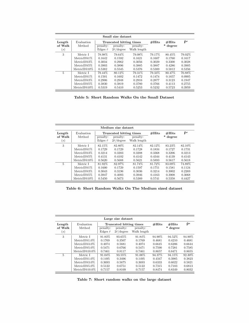
Exact parameter of random walks can be obtained by matrixmanipulation but this is costly in time and memory. There-fore we estimate the parameter using short random walks.We based our experiments around repeated short randomwalks from a given start. The details of these experimentsare given in Section 6. In common with our findings thatP 3 gave best results among matrix based methods, we findthat random walks of length 3 give best results. For s equalto 3 and 5, we compare the performance of the P s method,which computes the s-th power of matrix P , with the per-formance of the P s method, which estimates the s-th powerof P by simulating random walks of length s. For example,in the small dataset we can approximate P 3 with a rela-tive difference of 0.05 after 20n walk steps (See Equation 4).The large dataset reaches this accuracy in sublinear time(see Figures 3 and 5)

4. EVALUATION METHODOLOGYTo ensure reproducibility of results and to facilitate compar-ison between various recommender systems, each MovieLensdataset is partitioned into two parts: a training, or base, setB and a test set T . The test set is obtained by selecting10 random user-movie ratings for each user. The trainingset consists of all remaining ratings. To make this partition-ing feasible, the small dataset has more than 10 ratings pereach user. The medium and large datasets have at least 20ratings per each user.

The methodology for evaluating the performance of a rec-ommender system is to consider the training set as the in-formation about the past (which movies have been watched,and ranked, by each user) and the test set as the (hidden)information about who will watch what in the future. Arecommender system is run on the training set to computefor each user a ranking of movies, and then the computedrankings are compared with the test set. A better recom-mender system would be more effective in reconstructing thehidden information, that is, would give a closer fit betweenthe computed rankings and the test set. More precisely, foreach user u, the ranking of movies computed for this user

is compared with the set {m(u)1 ,m

(u)2 , . . . ,m

(u)tu} of the test

movies for this user. The pairs 〈u,m(u)1 〉, 〈u,m

(u)2 〉, . . . ,

〈u,m(u)tu〉 are this user’s ratings excluded from the training

set and included in the test set. A better recommender sys-

tem would place the movies m(u)i higher in the ranking. It

is not obvious, however, how the closeness between the com-puted rankings and the test set should be quantified and anumber of measures have been proposed.

Herlocker et al. [12] discusses different measures of the per-formance of ranking algorithms. Among the most commonones are the percentage of correctly placed pairs (used in [8,9]) and the number of hits in the top k recommendations.We use both these measures in this paper. To define thesemeasures, we assume the general evaluation methodology

described earlier (the bipartite graph G = (U ∪ I,R) par-titioned into the training set B and the test set T ), andwe use the following notation: |U | = p, |I| = q, |R| = r,

I(u) = {m ∈ I : 〈u,m〉 ∈ R} is the set of all items associ-

ated with user u, I(u)B = {m ∈ I : 〈u,m〉 ∈ B} is the set of

the training items for user u, I(u)T = {m ∈ I : 〈u,m〉 ∈ T} is

the set of the test items for user u, |I(u)| = iu, |I(u)B | = bu,

|I(u)T | = tu. For example, for a MovieLens dataset, I(u) is

the set of all movies watched (rated) by user u, while I(u)T is

the set of the movies watched by user u but put aside in thetest set. For all three MovieLens dataset, tu = 10 for eachuser u.

For a given ranking algorithm A, Rank (u) = 〈m(u)1 ,m

(u)2 ,. . .,

m(u)qu 〉 denotes the ranking of items computed for user u, and

m′ <u m′′ means that item m′ appears in Rank(u) before

item m′′ (so is ranked higher than item m′′).

Metric I: The number of correctly placed pairs

This measure requires that the ranking algorithm A com-putes for each user a full ranking, that is, a ranking whichincludes all items. Hence we assume qu = q, for each user u.To calculate the score for a given user u, consider all pairs

of items 〈m′,m′′〉, with m′ ∈ I(u)T and m′′ ∈ I \ I(u). Wesay that such pair 〈m′,m′′〉 is correctly placed, if m′ <u m

′′,that is, if the (test) item m′ is ranked higher than (appearsbefore) the item m′′. The score for user u is the percentageof correctly placed pairs:

|{〈m′,m′′〉 : m′ ∈ I(u)T , m′′ ∈ I \ I(u), m′ <u m′′}|tu(q − iu)

· 100%.

The score of the ranking algorithm is the average user score,over all users. If the tu test items for user u are the firstitems, in any order, in the ranking Rank(u) \ I(u)B , then thescore for this user is the perfect 100%. For the MovieLensdataset, the score of 100% means that the top tu moviesrecommended for user u, on the basis of the training set,are exactly the movies which this user has actually alreadywatched, but have been hidden in the test set.

Metric II: The number of hits in the top k recom-mendations

An alternative evaluation measure is the number of hits inthe top k recommendations. This measure is based on thesimple all-or-nothing concept of counting only the test itemswhich have made into the top k recommendations, ignoringtheir exact positions in the top k, and ignoring the positionsof the test items outside the top k. The parameter k is ei-ther an absolute value, usually ranging between 10 and 100,or a fraction of the total number of items, usually rangingbetween 1% and 10%. In this paper we use the relative val-ues for k since this is more appropriate when using datasetsof varied sizes. The number of hits is usually reported asthe fraction of the test items in the top k recommendations,

that is the fraction of the items from I(u)T which are among

the first k items in the list Rank(u) \ I(u)B .

5. MATRIX BASED METHODS5.1 Ranking algorithms

The input for the ranking methods is the bipartite graphG = (U ∪ I,R). The methods are general, but we describethem using the terminology of the MovieLens datasets, sincethe evaluation presented in [8, 9] and our evaluation arebased on those datasets. Thus we refer to U as the set ofusers, to I as the set of movies, and the edges in G showwhich movies the users have watched. A ranking algorithmcomputes for each user a ranking of movies.

Fouss et al. [8, 9] applied several ranking methods to thesmall 100K MovieLens dataset using Metric I to evaluatetheir performance. The methods which they used include:ranking by degree (MaxF), Hitting-time (Hit←, Hit→),Commute time (AVC) and Pseudo-Inverse Laplacian (L+).They reported that the simple degree based ranking per-formed reasonably well, scoring 85%, which is significantlyabove the 50% score of the random permutation. The de-gree based ranking is probably the simplest possible methodbased fully only on the popularity of individual movies andrequires little computation. The hitting time based rank-ings are considerably more costly to compute, but they didnot perform better than the degree based ranking. The hit-ting time ranking could only match the performance of thedegree based ranking, while the reverse hitting time rank-ing performed actually worse, scoring only 80%. The bestranking method was the L+ ranking, scoring 90%.

We have experimented with a number of ranking methods,looking for simple and intuitive methods which would match,or ideally exceed, the performance of the methods investi-gated in Fouss et al. [8, 9]. We include in this paper exper-imental results the five ranking methods mentioned aboveand considered in [8, 9], the ItemRank (IR) method de-scribed in [11], and the following methods.

The s-step random walk distribution (Ps) :

Movies that the user u has not watched are ranked basedon the probability distribution P s(u, .) of the random walkat step s, if u was the starting vertex. If P s(u,m′) >P s(u,m′′), then movie m′ is ranked higher than movie m′′.The matrix P s can be computed by raising the matrix P ofthe transition probabilities of the random walk on G to thepower of s.

Observe that only odd numbers s ≥ 3 should be considered:for a user u and a movie m not watched by u, the probabilityP s(u,m) can be positive only for an odd s ≥ 3. In thispaper we include experimental results only for the P 3 andP 5 rankings (the rankings based on the distribution of therandom walk after 3 and 5 steps, respectively), since theyperformed the best among the P s rankings.

Number of paths of length 3 (#3-Paths):

Movies that the user has not watched are ranked based onthe number of distinct paths of length 3 from that user tothe movies in graph G. A movie m with the greater numberof paths has a higher ranking. The numbers of paths oflength 3 can be simply computed as the third power of theadjacency matrix A.

Inverse Laplacian of the transition matrix (Z/πππ):

Matrix Z is defined by letting

Zij =∑t≥0

(P (t)(i, j)− πj

), (1)

where P (t)(i, j) is the probability that the random walkstarting at vertex i is at vertex j at step t, and π is thestationary distribution. Matrix Z appears in some identitiescharacterizing the parameters of the random walk. For ex-ample, Zjj/πj is the expected hitting time of vertex j fromthe stationary distribution; see Chapter 2 of Aldous andFill [6] for further details. For a user u, the Z/π methodranks the movies according to their Zu,m/πm values, withhigher values indicating higher ranks. It can be shown thatZij/πj is the expected hitting time of j from the station-ary distribution minus the expected hitting time of j fromi, that is,

Zij/πj =

(∑x

πxH(x, j)

)−H(i, j).

Matrix Z can be obtained from the inverse Laplacian of thetransition matrix P , as opposed to the inverse Laplacian ofthe adjacency matrix A used in [9]:

Z = (I − P + Π)−1 −Π,

where I is the identity matrix and Πij = πj . The details aregiven in Lovasz [17]. Since the sums (1) converge rapidly, theinverse Laplacian of the transition matrix P can be obtainedeasily by numeric means.

5.2 Implementation detailsIn this section, we discuss the technical issues that arisewhen implementing the ranking methods discussed above.

The scoring matrices for the hitting time (Hit→), reversehitting time (Hit←) and commute time (AVC) methods canbe obtained from the hitting time matrix H. Fouss et al. in[8, 9] suggest a method to compute this hitting time matrixthrough the pseudo-inverse of the Laplacian matrix (L+).However, this approach has a high computational cost. Inaddition to the computation of an inverse of a matrix, theformulas for the hitting times used in [8, 9] requires O(n3)arithmetic operations, where n is the size of a Laplacianmatrix. In order to compute the hitting time matrix Hfaster, we adopt the method presented in [17], which is basedon the following formulas.

X = (I − P + π)−1(J − 2rD−1)

H = X − (e ∗ λT )

where I is the identity matrix of size n, P is the transitionprobability matrix, π is stationary distribution, J is the ma-trix of ones of size n × n, r is the total number of edges,D is the diagonal matrix of vertex degrees, λ is the columnvector containing the diagonal entries of matrix X, and e isthe column vector of ones.

Matrix multiplication requires O(n2) space, therefore if thesize of graph increases, computing the P s matrix may re-quire impractical amount of memory space. For example,in the large 10M MovieLens dataset, there are 82, 248 nodesin total, therefore a naive approach of computing P 3 would

need 75 GB memory, or even 150GB, depending on the pre-cision required. To reduce the computational costs of bothtime and space, instead of computing the full matrix P s, wecompute the U × I part of this matrix (required for scoring)using the following formula.

P sU×I = PU×I (PI×U · PU×I)(s−1)/2 , for odd s, (2)

where PU×I and PI×U are the U × I and I × U parts ofmatrix P .

This improves the computation for the 100K and 1Mdatasets, but is not sufficient for the 10M dataset. For thislarge dataset, we split matrices PU×I and PI×U into 9 blocksand compute P sU×I by an appropriate sequence of multipli-cations and additions of these blocks.

5.3 Experimental results for matrix methodsIn this section we present our experimental results for thematrix based ranking methods described in Section 5.1. Allthree datasets discussed in Section 4 are used in the experi-ments. We used MATLAB for matrix based calculations.

Table 1 shows the performance of the ranking algorithmson the small 100K MovieLens dataset evaluated with themetric I (the percentage of correctly placed pairs) and themetric II (the number of hits in the top k). We obtainedthe same metric I scores as in [8, 9] for the methods con-sidered there. Regarding the additional methods, the P 3

ranking method turns out to perform very well, matchingthe performance of the L+ method.

Table 1 also shows the scores of the ranking algorithms ob-tained using the metric II. We varied the parameter k of thismetric – the number of top recommendations taken into ac-count – from 1% to 10%. It turns out that the relativeperformance of the ranking algorithms in our experiments isexactly the same in both metrics. The scores computed bythe metric II, however, seem to be easier to interpret.

For example, it is not immediately clear how significant thedifference between the metric I scores for the hitting timeranking (Hit→, 85%) and the reverse hitting time ranking(Hit←, 80%) is. However, the metric II scores in Table 1clearly show that the reverse hitting time ranking is muchweaker than the hitting time ranking. Metric II is also com-putationally easier than Metric I, since it does not involvesorting the rows of the computed ranking matrix.

Table 2 shows the performance of ranking algorithms on themedium 1M MovieLens dataset. The most interesting find-ing here is that P 3 has become the best method, overtakingslightly but clearly, the L+ method. We also observe thatthe performance of the MaxF and the hitting time methodsare almost the same on both datasets. The performance ofthe reverse hitting time method is somewhat better on thelarger dataset, but still clearly behind the other methods.

Table 3 shows the score of ranking algorithms obtained usingthe Metric I and Metric II for the large 10M MovieLensdataset. Note that for the large dataset, due to insufficientmemory space the ranking algorithms, Hit←, Hit←, AVC,L+, IR, and Z/π are not included from the experiments.

Small size Dataset

Evaluation MaxF Hit→ Hit← AVC L+L+L+ IR1 Z/πππ P3 P5 3-Paths

Metric I 85.79% 85.74% 80.45% 85.76% 90.94% 89.03% 85.72% 90.99%90.99%90.99% 88.19% 87.95%MetricII@1% 0.169 0.161 0.007 0.161 0.214 0.212 0.160 0.2610.2610.261 0.197 0.193MetricII@3% 0.294 0.293 0.051 0.294 0.445 0.376 0.292 0.4520.4520.452 0.362 0.350MetricII@5% 0.381 0.382 0.125 0.382 0.5820.5820.582 0.478 0.381 0.559 0.460 0.444MetricII@10% 0.543 0.543 0.341 0.544 0.7360.7360.736 0.637 0.542 0.699 0.616 0.609

Table 1: Small-size dataset (User, Movie).

Medium size Dataset

Evaluation MaxF Hit→ Hit← AVC L+L+L+ IR Z/πππ P3 P5 #3-Paths

Metric I 85.93% 85.93% 82.28% 85.93% 88.10% 88.04% 85.93% 89.62%89.62%89.62% 86.68% 87.35%MetricII@1% 0.173 0.173 0.039 0.173 0.198 0.206 0.076 0.2340.2340.234 0.181 0.198MetricII@3% 0.319 0.319 0.171 0.320 0.374 0.370 0.159 0.4160.4160.416 0.333 0.356MetricII@5% 0.409 0.409 0.279 0.409 0.466 0.464 0.211 0.5180.5180.518 0.425 0.449MetricII@10% 0.567 0.567 0.458 0.567 0.604 0.624 0.309 0.6710.6710.671 0.586 0.606

Table 2: Medium size dataset (User, Movie).

Large size Dataset

Evaluation MaxF P3 P5 #3-Paths

Metric I 93.94 95.9895.9895.98 94.64 94.69MetricII@1% 0.353 0.4810.4810.481 0.405 0.407MetricII@3% 0.569 0.6800.6800.680 0.604 0.607MetricII@5% 0.679 0.7780.7780.778 0.714 0.714MetricII@10% 0.816 0.8850.8850.885 0.839 0.842

Table 3: Large size dataset (User, Movie).

In order to compare the performance of ranking algorithmsin terms of the computational time, we have measured therunning time of ranking algorithms by applying the MAT-LAB tic-toc method. For the simplicity and fairness, everyalgorithm is measured from the moment that the trainingset is loaded into memory to the moment that algorithmsproduce (unsorted) ranking matrix. The measurements arerepeated 5 times for each algorithm. The average values arepresented in Table 4.

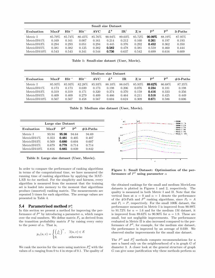
5.4 Parametrised method P3α

In this section we present a method for improving the per-formance of P s by introducing a parameter α, which rangesover the real numbers. We define matrix Pα as derived fromthe transition probability matrix P by raising every entryto the power of α. That is,

pα(u, v) =

{(1du

)α, ∃(u, v) ∈ E

0, otherwise

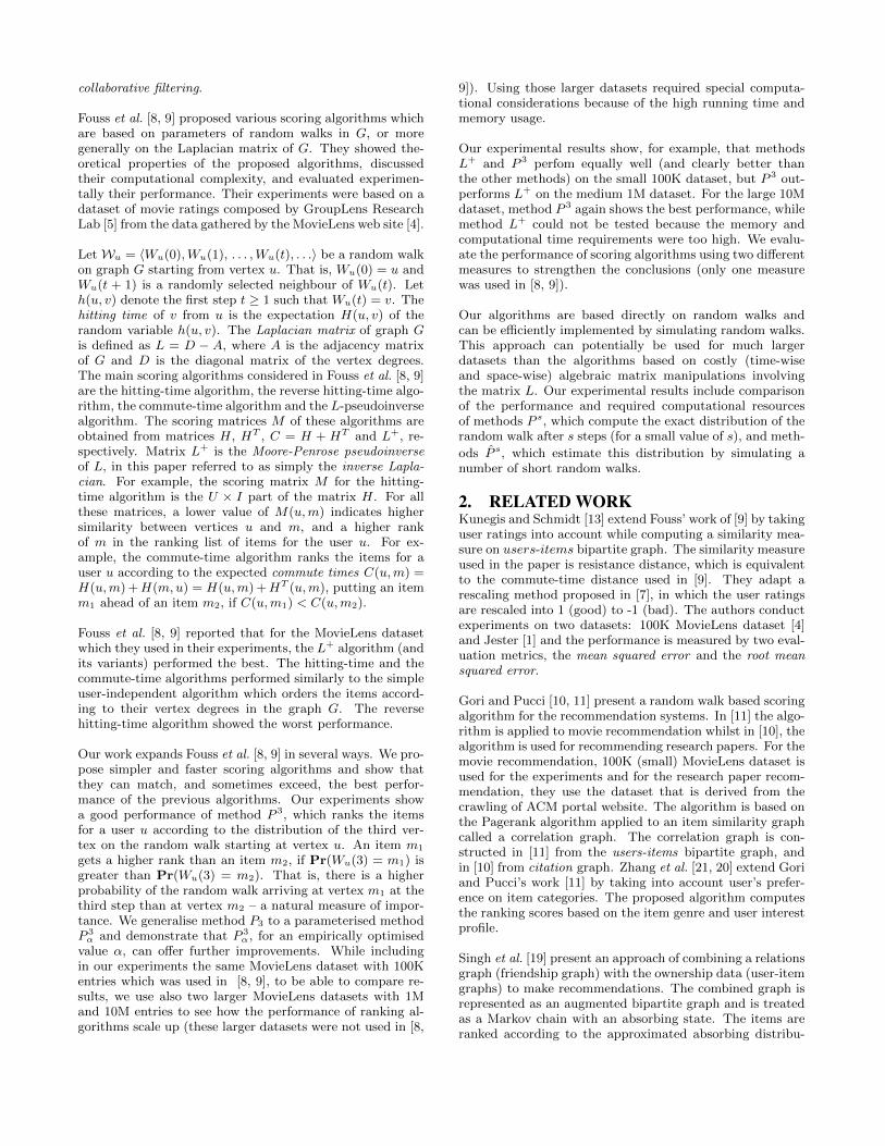
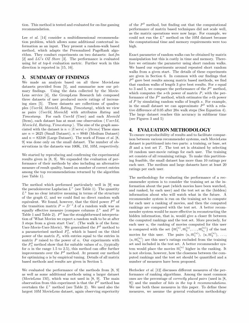
We rank the movies for the users using matrices P 3α with the

values of α ranging from 0 to 4 in steps of 0.1. The quality of

Figure 1: Small Dataset: Optimisation of the per-formance of P 3 using parameter α

the obtained rankings for the small and medium MovieLensdatasets is plotted in Figures 1 and 2, respectively. Thequality is measured in both Metric I and II. Note that thevertical lines at α = 0 and α = 1 denote the performanceof the #3-Path and P 3 ranking algorithms, since P0 = Aand P1 = P , respectively. For the small 100K dataset, theperformance measured in Metric I is improved from 90.99%to 91.72% for α = 1.6 and for the medium 1M dataset, itis improved from 89.62% to 90.90% for α = 1.9. These aresmall, but not negligible improvements. The performanceevaluated in Metric II is also increased compared to the per-formance of P 3, for example, for the medium size dataset,the performance is improved by an average of 0.039. Weobserved similar improvements for the small size dataset.

The P 3 and P 3α methods compute recommendations for a

user u based only on the neighbourhood of u in graph G ofdiameter 3. A closer look at the general structure of graphG can give some justification why these methods perform so

Dataset MaxF Hit→ Hit← AVC L+L+L+ IR Z/πππ P3 P5 #3-Paths

Small 0.15 3.48 3.48 3.48 2.25 32.91 3.10 1.44 1.69 0.40

Medium 0.39 89.24 89.24 89.24 64.42 852.26 77.20 46.70 60.03 11.51

Large 3.05 - - - - - - 1748.99 3504.47 1838.04

Table 4: Running time of the ranking algorithms (in seconds).

Figure 2: Medium Dataset: Optimisation of the per-formance of P 3 using parameter α

well. The diameter of G is small – for example, the trainingset subgraph for the small MovieLens dataset has diameter6, and on average 70% of the users are at distance 2 from agiven user. Another evident characteristic of the MovieLensdatasets is their relatively high density. For example, theaverage degree of a user in the training set of the smallMovieLens dataset is 95. Thus another interesting questionis how the ranking algorithms ”scale down”when the densityof the dataset decreases.

6. RANKING METHODS BASED ON SIM-ULATION OF RANDOM WALKS

Ranking algorithms based on matrix manipulations havetheir natural limit: the sizes of the matrices may quicklybecome too large to fit in the computer memory. Even ifthe graph G modelling the dataset is sparse, matrix opera-tions involving the adjacency matrix can easily lead to densematrices. For example, the pseudoinverse matrix L+ and thehitting time matrixH are both dense. We did not have prob-lems with running the ranking algorithms from the previoussection on the small MovieLens dataset, but some techni-cal issues of insufficient memory started appearing when wemoved on to the medium size dataset (the MovieLens 1Mset), and became a major obstacle for computing matricesin the largest MovieLens dataset.

An alternative approach is to gather information about thestructure of a graph from simulations of random walks in thisgraph. For example, the hitting times used in the rankingmethods in the previous section can obviously be estimatedby simulating random walks. Such simulations require onlyO(r) space, to store the adjacency lists of the graph, withr � n2 for sparse graphs (n is the number of vertices andr is the number of edges). Furthermore, the computationcan be organised in a distributed manner, if the graph is

Figure 3: Convergence on small dataset

scattered over a network.

6.1 Data captureWe consider ranking methods which compute the ranking ofitems for a user u on the basis of the information gatheredby random walks starting from vertex u. To obtained rank-ing algorithms which are not only space efficient but alsotime efficient, we set the limit of n on the total number ofsteps of all random walks performed for one user (called the“budget”). That way the ranking lists for all users can becomputed in O(n2) time, beating the time of algebraic oper-ations on n× n matrices. The required time to produce therecommendation per user grows linearly with the budgets.

More precisely, we perform w = n/s random walks startingfrom a given vertex u, with each walk having s steps, forsome fixed parameter s. Taking into account all w walks,we rank vertices on the basis of how often they are hit onaverage, or how quickly they are hit on average. For eachvertex v and each random walk i = 1, 2, . . . , w, we keep thefollowing information: (a) the step sv(i) when vertex v wasvisited by walk i for the first time. (b) the indicator nv(i),which is equal to 1, if vertex v was visited by walk i, and 0otherwise, and (c) the degree d(v) of vertex v.

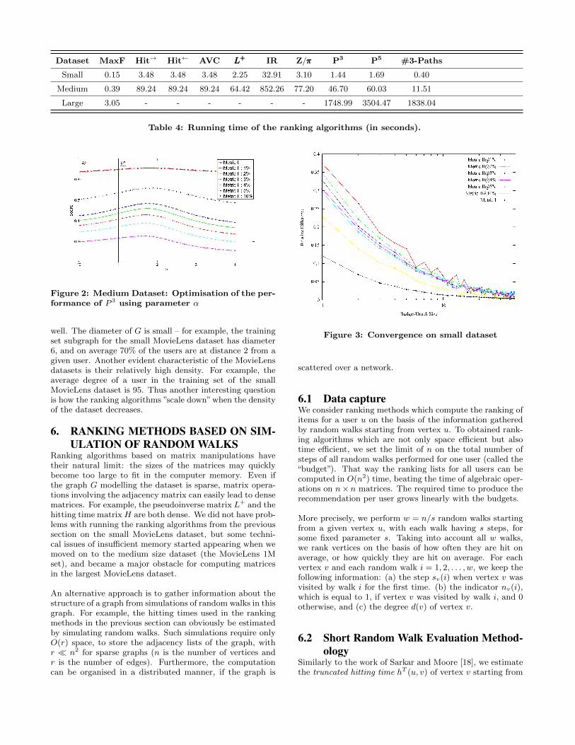
6.2 Short Random Walk Evaluation Method-ology

Similarly to the work of Sarkar and Moore [18], we estimatethe truncated hitting time hT (u, v) of vertex v starting from

vertex u by

1

w

w∑i=1

sv(i). (3)

To use this estimator, we have to decide what should bethe value of sv(i), if vertex v was not visited during walk i.Vertices which have not been visited by any of the walks arenot ranked (or they are put in arbitrary order at the endof the ranking list, if a full ranking list is required), so wedo not need to worry about their sv(i) values. We considernow a vertex v which was visited by some walks, but was notvisited by, say, walk i. A choice of sv(i) = 0 seems incorrect,as this would imply v = u. Some hitting time penalty shouldbe imposed for unvisited vertices, and we experimented withvarious values for this penalty. (a) Set the penalty to m, ourestimate of the number of edges incident with the subgraphwe can visit in s steps. (b) Set the penalty to 2m/d(v) wherem is the estimated number of edges. The reasoning behindthis penalty is to approximate the first hitting time fromstationarity of a vertex. We do not use the total number ofedges of a graph to cover the cases when this is unknown.The value m is our best estimate of the size of the sub-graphwe are expected to see within s steps, and approximates thenumber of edges in the breadth first search tree of depths+ 1 (c) Set the penalty to s, the walk length. This penaltyused in [18]. (d) Do not impose any penalty (set the penaltyto zero). We include this option in our experiments as areference point.

Having estimated hT (u, v) with (3) and using one of theabove penalties, we can rank the movies in ascending orderof their hT (u, v) values.

In addition to estimates of hT (u, v) we rank movies based onthe number of times they were hit on average. We calculatethe average number of hits of a vertex v from vertex u as

n(u, v) =1

w

w∑i=1

nv(i).

For example, if a movie m is hit w/2 times by w walks,then the number of hits is 0.5. Intuitively, movies whichwere hit often are more relevant to a user and should beranked higher. Movies are ranked for recommendation inthe descending order according to their average number ofhits. We also consider some heuristics for re-weighting ofaverage number of hits, such as (number of hits)*(degree).

We can also rank movies based on an estimate of the sstep transition probability. We can estimate this simply bycounting P (k)(u, v) – the number of walks which hit vertexv at step s divided by the total number of walks w. If welet the number of walks increase to infinity, P (s)(u, v) con-verges to P s(u, v). We rank movies in the descending order

of values P (s)(u, v).

6.3 Experimental results for random walkmethods

In order to estimate random walk properties without us-ing matrix operations we made use of many short randomwalks of various lengths. The experiments were ran on apersonal computer with an Intel Quad core CPU at 3 GHz(specifically Intel Core 2 Quad Q9650) and 8 GB DDR2-800

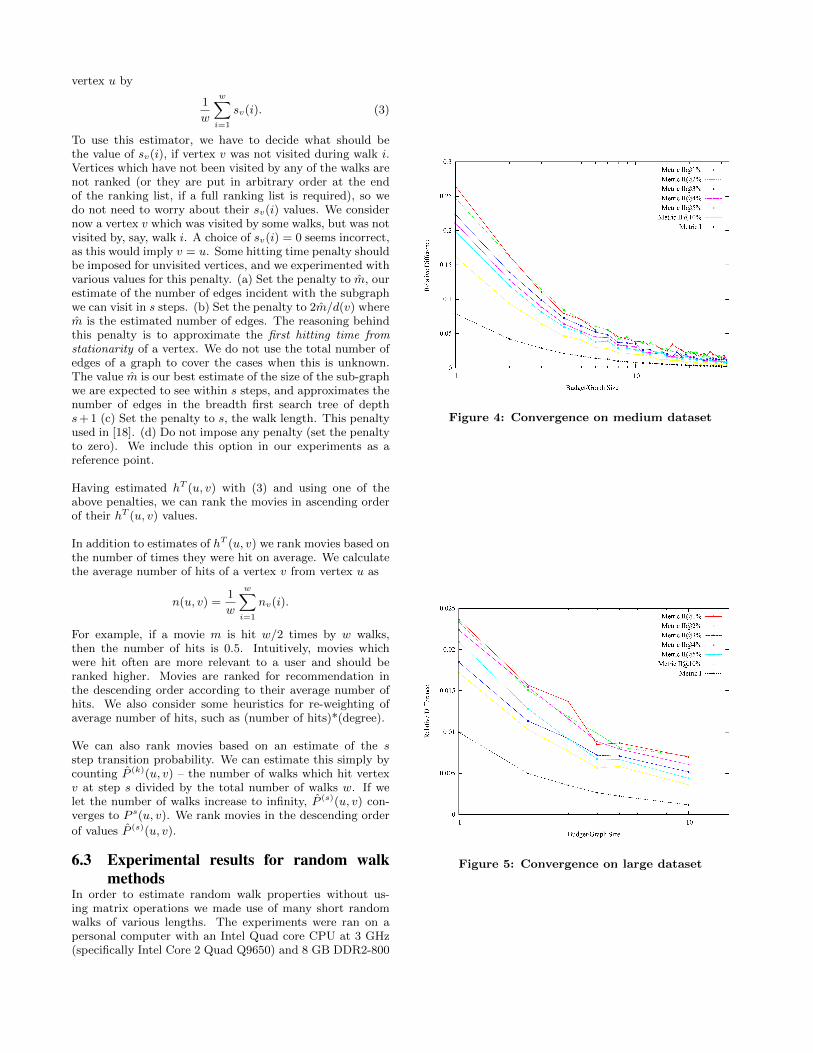
Figure 4: Convergence on medium dataset

Figure 5: Convergence on large dataset

Small size dataset

Length Evaluation Truncated hitting times #Hits #Hits Ps

of Walk Method penalty: penalty: penalty: * degree(s) Edges r 2r/degree Walk length

3 Metric I 78.98% 79.64% 79.08% 79.17% 80.45% 79.02%MetricII@1% 0.1642 0.1592 0.1621 0.1607 0.1760 0.1617MetricII@3% 0.3034 0.2962 0.3056 0.3029 0.3300 0.3028MetricII@5% 0.3903 0.3896 0.3885 0.3887 0.4286 0.3905MetricII@10% 0.5382 0.5545 0.5376 0.5389 0.5812 0.5356


Table 5: Short Random Walks On the Small Dataset

Medium size dataset





Table 6: Short Random Walks On The Medium sized dataset

Large size dataset



3 Metric I 91.83% 93.65% 91.84% 94.90% 94.52% 94.90%[email protected]% 0.1769 0.3507 0.1769 0.4681 0.4210 [email protected]% 0.4074 0.5681 0.4074 0.6645 0.6206 [email protected]% 0.5471 0.6766 0.5471 0.7590 0.7281 [email protected]% 0.7461 0.8117 0.7461 0.8657 0.8471 0.8655

5 Metric I 91.04% 93.55% 91.06% 94.37% 94.15% 92.30%[email protected]% 0.1495 0.3496 0.1495 0.4347 0.3985 [email protected]% 0.3693 0.5675 0.3693 0.6333 0.6022 [email protected]% 0.5122 0.6751 0.5122 0.7315 0.7103 [email protected]% 0.7157 0.8109 0.7157 0.8474 0.8349 0.8032

Table 7: Short random walks on the large dataset

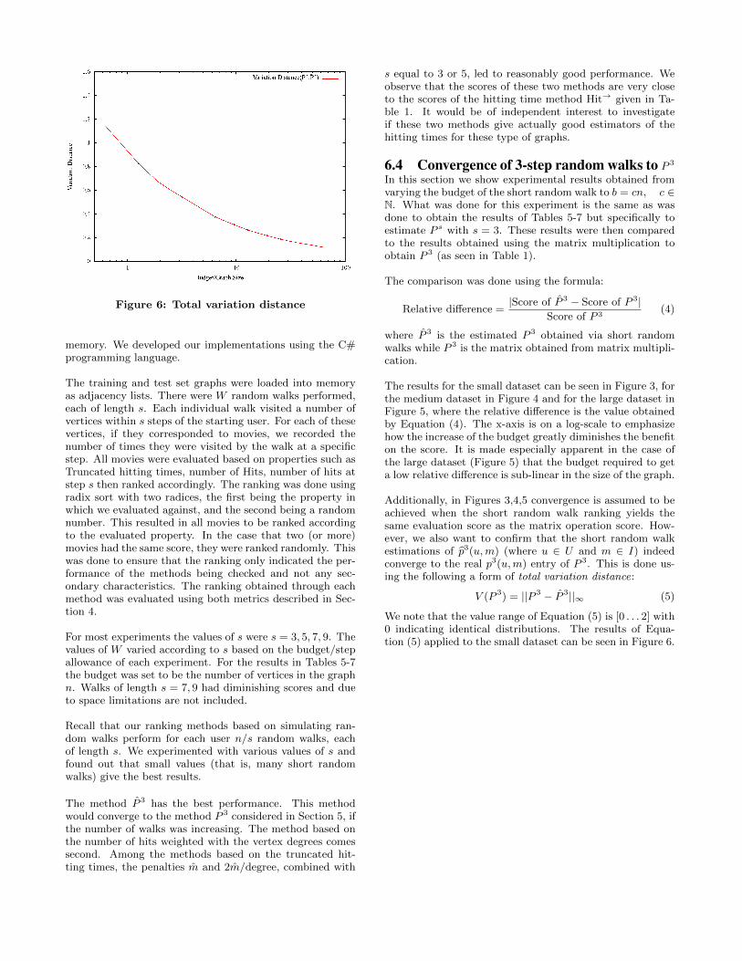
Figure 6: Total variation distance

memory. We developed our implementations using the C#programming language.

The training and test set graphs were loaded into memoryas adjacency lists. There were W random walks performed,each of length s. Each individual walk visited a number ofvertices within s steps of the starting user. For each of thesevertices, if they corresponded to movies, we recorded thenumber of times they were visited by the walk at a specificstep. All movies were evaluated based on properties such asTruncated hitting times, number of Hits, number of hits atstep s then ranked accordingly. The ranking was done usingradix sort with two radices, the first being the property inwhich we evaluated against, and the second being a randomnumber. This resulted in all movies to be ranked accordingto the evaluated property. In the case that two (or more)movies had the same score, they were ranked randomly. Thiswas done to ensure that the ranking only indicated the per-formance of the methods being checked and not any sec-ondary characteristics. The ranking obtained through eachmethod was evaluated using both metrics described in Sec-tion 4.

For most experiments the values of s were s = 3, 5, 7, 9. Thevalues of W varied according to s based on the budget/stepallowance of each experiment. For the results in Tables 5-7the budget was set to be the number of vertices in the graphn. Walks of length s = 7, 9 had diminishing scores and dueto space limitations are not included.

Recall that our ranking methods based on simulating ran-dom walks perform for each user n/s random walks, eachof length s. We experimented with various values of s andfound out that small values (that is, many short randomwalks) give the best results.

The method P 3 has the best performance. This methodwould converge to the method P 3 considered in Section 5, ifthe number of walks was increasing. The method based onthe number of hits weighted with the vertex degrees comessecond. Among the methods based on the truncated hit-ting times, the penalties m and 2m/degree, combined with

s equal to 3 or 5, led to reasonably good performance. Weobserve that the scores of these two methods are very closeto the scores of the hitting time method Hit→ given in Ta-ble 1. It would be of independent interest to investigateif these two methods give actually good estimators of thehitting times for these type of graphs.

6.4 Convergence of 3-step random walks to P 3

In this section we show experimental results obtained fromvarying the budget of the short random walk to b = cn, c ∈N. What was done for this experiment is the same as wasdone to obtain the results of Tables 5-7 but specifically toestimate P s with s = 3. These results were then comparedto the results obtained using the matrix multiplication toobtain P 3 (as seen in Table 1).

The comparison was done using the formula:

Relative difference =|Score of P 3 − Score of P 3|

Score of P 3(4)

where P 3 is the estimated P 3 obtained via short randomwalks while P 3 is the matrix obtained from matrix multipli-cation.

The results for the small dataset can be seen in Figure 3, forthe medium dataset in Figure 4 and for the large dataset inFigure 5, where the relative difference is the value obtainedby Equation (4). The x-axis is on a log-scale to emphasizehow the increase of the budget greatly diminishes the benefiton the score. It is made especially apparent in the case ofthe large dataset (Figure 5) that the budget required to geta low relative difference is sub-linear in the size of the graph.

Additionally, in Figures 3,4,5 convergence is assumed to beachieved when the short random walk ranking yields thesame evaluation score as the matrix operation score. How-ever, we also want to confirm that the short random walkestimations of p3(u,m) (where u ∈ U and m ∈ I) indeedconverge to the real p3(u,m) entry of P 3. This is done us-ing the following a form of total variation distance:

V (P 3) = ||P 3 − P 3||∞ (5)

We note that the value range of Equation (5) is [0 . . . 2] with0 indicating identical distributions. The results of Equa-tion (5) applied to the small dataset can be seen in Figure 6.

7. REFERENCES[1] Anonymous ratings data from the jester online joke

recommender system.http://goldberg.berkeley.edu/jester-data.

[2] Last.fm. http://www.last.fm/.

[3] Lg u+ oz store. http://ozstore.uplus.co.kr/.

[4] Movielens. http://movielens.umn.edu.

[5] Movielens data sets. GroupLens Research Lab, Dept.Computer Science and Engineering, University ofMinnesota. http://www.grouplens.org/node/73.

[6] D. Aldous and J. A. Fill. Reversible markov chainsand random walks on graphs. http://stat-www.berkeley.edu/pub/users/aldous/RWG/book.html,1995.

[7] D. Billsus and M. J. Pazzani. Learning collaborativeinformation filters. In ICML, pages 46–54, 1998.

[8] F. Fouss, A. Pirotte, J.-M. Renders, and M. Saerens.Random-walk computation of similarities betweennodes of a graph with application to collaborativerecommendation. IEEE Trans. Knowl. Data Eng.,19(3):355–369, 2007.

[9] F. Fouss, A. Pirotte, and M. Saerens. A novel way ofcomputing similarities between nodes of a graph, withapplication to collaborative recommendation. InA. Skowron, R. Agrawal, M. Luck, T. Yamaguchi,P. Morizet-Mahoudeaux, J. Liu, and N. Zhong,editors, Web Intelligence, pages 550–556. IEEEComputer Society, 2005.

[10] M. Gori and A. Pucci. Research paper recommendersystems: A random-walk based approach. In WebIntelligence, pages 778–781, 2006.

[11] M. Gori and A. Pucci. Itemrank: A random-walkbased scoring algorithm for recommender engines. InIJCAI, pages 2766–2771, 2007.

[12] J. L. Herlocker, J. A. Konstan, L. G. Terveen, John,and T. Riedl. Evaluating collaborative filteringrecommender systems. ACM Transactions onInformation Systems, 22:5–53, 2004.

[13] J. Kunegis and S. Schmidt. Collaborative filteringusing electrical resistance network models. InIndustrial Conference on Data Mining, pages 269–282,2007.

[14] S. Lee, S. il Song, M. Kahng, D. Lee, and S. goo Lee.Random walk based entity ranking on graph formultidimensional recommendation. In RecSys, pages93–100, 2011.

[15] S. Lee, S. Park, M. Kahng, and S. goo Lee. Pathrank:a novel node ranking measure on a heterogeneousgraph for recommender systems. In CIKM, pages1637–1641, 2012.

[16] S. Lee, S. Park, M. Kahng, and S. goo Lee. Pathrank:Ranking nodes on a heterogeneous graph for flexiblehybrid recommender systems. Expert Syst. Appl.,40(2):684–697, 2013.

[17] L. Lovasz. Random walks on graphs: A survey. BolyaiSociety Mathematical Studies, 2:353–397, 1996.

[18] P. Sarkar and A. W. Moore. A tractable approach tofinding closest truncated-commute-time neighbors inlarge graphs. In R. Parr and L. C. van der Gaag,editors, UAI, pages 335–343. AUAI Press, 2007.

[19] A. P. Singh, A. Gunawardana, C. Meek, and A. C.Surendran. Recommendations using absorbing randomwalks. North East Student Colloquium on ArtificialIntelligence (NESCAI), 2007.

[20] L. Zhang, J. Xu, and C. Li. A random-walk basedrecommendation algorithm considering itemcategories. Neurocomputing, 120(0):391 – 396, 2013.

[21] L. Zhang, K. Zhang, and C. Li. A topical pagerankbased algorithm for recommender systems. In SIGIR,pages 713–714, 2008.

Documents

Random Walks in Recommender Systems: Exact Computation …